Analytic models of dust temperature in high-redshift galaxies

Abstract

We investigate physical reasons for high dust temperatures ($T_{\mathrm{dust}}\gtrsim 40$ K) observed in some high-redshift ($z>5$) galaxies using analytic models. We consider two models that can be treated analytically: the radiative transfer (RT) model, where a broad distribution of values for $T_{\mathrm{dust}}$ is considered, and the one-tempearture (one-$T$) model, which assumes uniform $T_{\mathrm{dust}}$. These two extremes serve to bracket the most realistic scenario. We adopt the Kennicutt–Schmidt (KS) law to relate stellar radiation field to gas surface density, and vary the dust-to-gas ratio. As a consequence, our model is capable of predicting the relation between the surface density of star formation rate ($\Sigma_{\mathrm{SFR}}$) or dust mass ($\Sigma_{\mathrm{dust}}$) and $T_{\mathrm{dust}}$. We show that the high $T_{\mathrm{dust}}$ observed at $z\gtrsim 5$ favour low dust-to-gas ratios ($\lesssim 10^{-3}$). An enhanced star formation compared with the KS law gives an alternative explanation for the high $T_{\mathrm{dust}}$. The dust temperatures are similar between the two (RT and one-$T$) models as long as we use ALMA Bands 6–8. We also examine the relation among $\Sigma_{\mathrm{SFR}}$, $\Sigma_{\mathrm{dust}}$ and $T_{\mathrm{dust}}$ without assuming the KS law, and confirm the consistency with the actual observational data at $z>5$. In the one-$T$ model, we also examine a clumpy dust distribution, which predicts lower $T_{\mathrm{dust}}$ because of the leakage of stellar radiation. This enhances the requirement of low dust abundance or high star formation efficiency to explain the observed high $T_{\mathrm{dust}}$.

1 Introduction

The interstellar medium (ISM) of galaxies usually contains dust grains, which play an important role in various physical processes on galactic or sub-galactic scales. Dust absorbs and scatters the radiation from stars, and reradiates it at infrared (IR)–submillimetre (submm) wavelengths (e.g. Buat & Xu, 1996; Calzetti et al., 2000). In this way, dust strongly modifies the spectral energy distribution (SED) of interstellar radiation field and that of galaxy emission (e.g. Silva et al., 1998; Takagi et al., 2003; Takeuchi et al., 2005). This means that a part of star formation activity in a galaxy can only be traced in the IR–submm (e.g. Kennicutt, 1998a; Inoue et al., 2000), and that when we extract galaxy properties (stellar mass, age, etc.) from SED fitting, it is crucial to appropriately consider dust extinction and reemission (e.g. da Cunha et al., 2008; Boquien et al., 2019; Abdurro’uf et al., 2021; Ferrara et al., 2022). When dust shields ultraviolet (UV) light, it emits photoelectrons, contributing to the heating of the ISM (e.g. Tielens, 2005). Dust surfaces are reaction sites for molecular hydrogen formation (e.g. Gould & Salpeter, 1963; Cazaux & Tielens, 2004). This makes cold star-forming regions rich in H₂ molecules (Yamasawa et al., 2011; Chen et al., 2018; Romano et al., 2022). Dust also induces fragmentation in the star formation process, determining a characteristic mass of a star. Trough this process, dust also affects the stellar initial mass function (IMF; e.g. Omukai et al. 2005; Schneider et al. 2006).

The above effects of dust may have already been important at high redshift ($z$) since some galaxies are already dusty at $z>5$ (e.g. Capak et al., 2015; Burgarella et al., 2020; Fudamoto et al., 2021). The redshift frontier of dust observation has been expanded to $z>5$ (e.g. Dayal & Ferrara, 2018) because of the high capability of the Atacama Large Millimetre/submillimetre Array (ALMA). For a ’typical’ population of high-redshift galaxies, Lyman break galaxies (LBGs), dust emission has been detected even at $z>7$ (e.g. Watson et al., 2015; Laporte et al., 2017; Tamura et al., 2019; Hashimoto et al., 2019; Schouws et al., 2022; Inami et al., 2022), although we should also note that most LBGs at such high redshift have too weak dust emission to be detected by ALMA with a limited time of integration (e.g. Bouwens et al., 2016; Fudamoto et al., 2020).

Observationally, correctly estimating the dust mass is of fundamental importance. The dust masses derived from ALMA observations for high-redshift galaxies are highly uncertain because it is difficult to obtain precise dust temperature. Some studies succeeded in obtaining dust temperatures in LBGs at $z\gtrsim 5$ from multi-wavelength ALMA data. A1689-zD, detected with ALMA in Band 6 (1,300 $\micron$; Watson et al. 2015), is later followed up in Band 7 (870 $\micron$) by Knudsen et al. (2017), who obtained a dust temperature of 35–45 K, higher than those in nearby spiral galaxies ($\sim 20$–25 K; e.g. Draine & Li 2007). The high dust temperature of this object was confirmed by further detections in Band 8 (730 $\micron$; Inoue et al. 2020) and Band 9 (430 $\micron$; Bakx et al. 2021). Including such short wavelengths may be important to trace LBGs with high dust temperatures (Chen et al., 2021), as also demonstrated for the above object by Bakx et al. (2021). Burgarella et al. (2020) compiled ALMA detections of LBGs at various $z(>5)$, which enabled them to statistically trace dust emission SEDs at different restframe wavelengths (see also Nanni et al., 2020; Burgarella et al., 2022), and obtained dust temperatures of 40–70 K. Faisst et al. (2020) estimated dust temperatures of four LBGs at $z\sim 5.5$ as 30–43 K (see also Faisst et al., 2017). Bakx et al. (2020) obtained an even higher dust temperature for a LBG at $z=8.31$ ($>80$ K). Sommovigo et al. (2021, 2022) indirectly derived dust temperatures by utilizing some empirical relations involving [C ii] 158 $\micron$ emission, obtaining similar dust temperatures to the above ($\sim 30$–70 K) for a sample of $z>5$ galaxies. These values imply not only systematically warmer dust than in nearby galaxies but also a large variety in dust temperature at $z\gtrsim 5$.

The physical reason for high dust temperature is worth clarifying because it may give us a clue to the evolution of star formation activities and dust properties. In fact, a tendency of increasing dust temperature with redshift is observed at $z\lesssim 4$ (Béthermin et al., 2015; Schreiber et al., 2018; Béthermin et al., 2020; Bouwens et al., 2020; Faisst et al., 2020; Viero et al., 2022), although we need to be careful about the selection effect (Lim et al., 2020). Cosmological simulations also predict high dust temperature at high redshift (Behrens et al., 2018; Aoyama et al., 2019; Ma et al., 2019; Liang et al., 2019; Vijayan et al., 2022; Pallottini et al., 2022). The tendency of higher dust temperature at higher redshift could be related to increasing star formation efficiencies (or equivalently decreasing gas-depletion time-scales; Magnelli et al. 2014; Sommovigo et al. 2022). High dust temperature could also be realized if star-forming regions have concentrated, compact morphologies (Ferrara et al., 2017; Behrens et al., 2018; Liang et al., 2019; Sommovigo et al., 2020; Pallottini et al., 2022). Sommovigo et al. (2022) also considered the effect of dust mass (as taken into account by other theoretical studies; e.g. Hirashita & Ferrara 2002) in determining the dust temperature, which effectively includes shielding of stellar light; that is, as the dust mass increases, the dust shields the stellar radiation and lowers the dust heating per dust mass. This means that low dust abundance, as well as high stellar radiation intensity, is important for rising dust temperature towards high redshift.

Since the above conclusions are derived in different contexts, we here aim at further focusing on the possible essential quantities – dust abundance and stellar radiation field – that affect the dust temperature. This serves to clarify the physical conditions that could explain the observed high dust temperatures at high redshift. We formulate the problem by focusing on physical processes that determine the dust temperature – heating from stellar radiation and dust radiative cooling. The balance between these two processes is treated by an equilibrium condition as in Ferrara et al. (2017) and Sommovigo et al. (2020). In other words, this paper investigates how the equilibrium condition is affected by the star formation activities and dust properties. To make the physical processes transparent, we treat the problem analytically, which is complementary to some numerical simulations mentioned above. The transparency of our approach is also useful to examine the dust shielding effects with a variety of dust distribution geometries and dust properties (grain sizes and compositions), further serving to examine how robustly dust abundance and stellar radiation field affect the dust temperature. Utilizing the developed analytic models, we also address the effects of grain compositions and grain size distribution, which are suggested to influence the observational properties of galaxies at UV and IR wavelengths (Yajima et al., 2014).

In this paper, we focus on $z>5$, where the current redshift frontier of dust observation is located. Nevertheless, we emphasize that the physical processes treated in this paper are common for any redshift. Thus, the conclusion drawn this paper is qualitatively applicable to galaxies at $z<5$. In particular, we plan a separate study for local galaxies by using the framework developed in this paper to further test our theoretical predictions (Chiang et al., in preparation). Focusing on a certain range of redshift would be useful to minimize the variation in redshift-dependent physical processes such as redshift evolution of gas-depletion time (Sommovigo et al., 2022), and systematic difference in stellar populations.

This paper is organized as follows. We explain the models for dust temperature in Section 2. We show the results in Section 3. We discuss some further issues, especially dependence on various parameters in Section 4. Section 5 concludes this paper. We adopt the following cosmological parameters: $\Omega_{\Lambda}=0.7$, $\Omega_{\mathrm{M}}=0.3$, and $H_{0}=70$ km s^-1 Mpc^-1.

2 Model

In this paper, we develop analytic models for dust temperature in a galaxy. To make an analytic treatment possible, we consider the following two extremes, which simplify the problem but still catch the essential physical factors affecting the dust temperature: (i) one is the case where we consider a distribution of values for the dust temperature, while (ii) the other assumes a single dust temperature value. We refer these models as the (i) radiative transfer (RT) model and (ii) one-temperature (one-$T$) model, respectively. The first model solves radiative transfer in a simple dust–stars geometry, while the second could treat another complexity – dust distribution geometry. Two models are complementary, and catch different physical aspects that vary the dust temperature under a fixed star formation activity in a galaxy.

In this paper we do not explicitly consider the effect of the cosmic microwave background (CMB) on the dust temperature (e.g. da Cunha et al., 2013) since it is redshift-dependent. Practically, the CMB sets a floor for the dust temperature; thus, any dust temperature below the CMB temperature, $2.73(1+z)$ K, is not physically permitted. However, since we are mainly interested in galaxies whose observed dust temperatures are significantly higher than the CMB temperature, the CMB does not affect our discussions and conclusions. Thus, we do not apply the redshift-dependent correction for the CMB temperature so that we do not have to specify the redshift for each result. Note that the background (including the CMB) is already subtracted from observational data used for comparison.

2.1 Basic setup

2.1.1 Galaxy properties

We represent the masses of dust, gas, and stars by their surface densities, denoted as $\Sigma_{\mathrm{dust}}$, $\Sigma_{\mathrm{gas}}$ and $\Sigma_{\star}$, respectively. A quantity per surface area is convenient since the dust temperature is determined by the radiation intensity, which has the same dimension as the surface brightness (luminosity per surface area). For simplicity, we assume that the dust, gas and stars are distributed in a uniform disc so that the above three quantities represent the galaxy properties. Although our formulation implicitly assumes disc geometry, we expect that our results are not strictly limited to discs because the dust heating radiation in a galaxy has on average an intensity on the order of $\sim L/(\pi R^{2})$, where $L$ and $R$ represent the stellar luminosity and the optical galaxy size, respectively. In particular, the geometry factor causes an uncertainty of at most factor 4 ($4\pi$ instead of $\pi$ in spherical shell geometry; e.g. Inoue et al. 2020), which affects the dust temperature only by a factor of $\sim 4^{1/6}\sim 1.26$ at most. Thus, our results could be applied to any geometry with a 20–30 per cent uncertainty in the dust temperature. Since we are interested in normal LBGs, we neglect the contribution from AGN heating (see e.g. Di Mascia et al., 2021, for the effect of AGN heating in high-redshift galaxies). We also neglect small-scale inhomogeneity that could not be included in our treatment of smooth surface densities (as commented in Section 4.3).

It is empirically established that the SFR is tightly related to the gas mass. This relation is described by the Kennicutt–Schmidt (KS) law as (Kennicutt, 1998b)

$$\left(\frac{\Sigma_{\mathrm{SFR}}}{\mathrm{M_{\sun}~{}yr^{-1}~{}kpc^{-2}}}\right)=1.0\times 10^{-12}\kappa_{\mathrm{s}}\left(\frac{\Sigma_{\mathrm{gas}}}{\mathrm{M_{\sun}~{}kpc^{-2}}}\right)^{1.4},$$ (1)

where $\Sigma_{\mathrm{SFR}}$ is the surface density of the SFR, and $\kappa_{\mathrm{s}}$ is the burstiness parameter. Following Ferrara et al. (2019) and Sommovigo et al. (2021), we include the correction factor $\kappa_{\mathrm{s}}$ explicitly, and we adopt $\kappa_{\mathrm{s}}=1$ for the default KS law. We also define the formed stellar mass, $\Sigma_{\star,0}$, as

$$\Sigma_{\star,0}=\Sigma_{\mathrm{SFR}}\tau_{\star},$$ (2)

where $\tau_{\star}$ is the age of the star formation activity. For simplicity, we assume a constant SFR within the duration $\tau_{\star}$. The surface luminosity density (stellar luminosity per surface area per frequency $\nu$), $\mathcal{I}_{\star\nu}$, is calculated as

$$\mathcal{I}_{\star\nu}=\Sigma_{\star,0}\ell_{\nu},$$ (3)

where $\ell_{\nu}$ is the luminosity density per formed stellar mass, and is calculated using a spectral synthesis model.

To calculate the SED per stellar mass ($\ell_{\nu}$), we use starburst99 (Leitherer et al., 1999) with a constant SFR and an age of $\tau_{\star}$. For simplicity, we fix the stellar SED and assume $\tau_{\star}\sim 10^{8}$ yr, which is roughly a typical stellar age for high-redshift LBGs (Liu & Hirashita, 2019, and references therein). Since UV radiation, which saturates in $\sim 10^{8}$ yr for a constant SFR, is the dominant source of dust heating (Buat & Xu, 1996), the resulting dust temperature is not sensitive to the adopted age as long as $\tau_{\star}\gtrsim 10^{8}$ yr. Since we are interested in an early phase of metal enrichment, we set the stellar metallicity to a sub-solar value, 0.008 ($\sim 1/2$ Z_⊙). Although we consider a wide range in the dust-to-gas ratio (note that the gas-phase metallicity is not used in our model), we fix the stellar metallicity, since it has much less impact than other parameters (e.g. dust-to-gas ratio) on the dust temperature. We adopt the Kroupa initial mass function (Kroupa, 2002) with a stellar mass range of 0.1–100 M_☉.

2.1.2 Dust properties

To make the problem analytically tractable, we neglect scattering, and only consider absorption by dust. Scattering could raise the chance of absorption because it effectively increases the path length of the photons. However, the cross-section for scattering is at most comparable to that of absorption, so that the absorbed energy increases by a factor of $\sim$2 at most. The dust temperature, which depends on the absorbed energy to the power $\sim 1/6$, does not change significantly. Changing other parameters such as dust-to-gas ratio, which increases the dust opacity proportionally, has a larger impact on the dust temperature. Thus, neglecting scattering does not influence our conclusions in this paper.

The mass absorption coefficient (absorption cross-section per gas mass), $\kappa_{\mathrm{g,abs}}(\nu)$, is evaluated, assuming compact spherical grains, as

$$\kappa_{\mathrm{g,abs}}(\nu)=\mathcal{D}\,\frac{\int_{0}^{\infty}\pi a^{2}Q_{\mathrm{abs}}(a,\,\nu)n(a)\,\mathrm{d}a}{\int_{0}^{\infty}\frac{4}{3}\pi a^{3}sn(a)\,\mathrm{d}a},$$ (4)

where $\mathcal{D}$ is the dust-to-gas ratio, $a$ is the grain radius, $Q_{\mathrm{abs}}(a,\,\nu)$ is the ratio of absorption to geometrical cross-sections, $s$ is the dust material density, and $n(a)$ is the grain size distribution, which is defined such that $n(a)\,\mathrm{d}a$ is the number density of grains in the radius range from $a$ to $a+\mathrm{d}a$. The absorption cross-section, specifically $Q_{\mathrm{abs}}(a,\,\nu)$, is calculated using the Mie theory (Bohren & Huffman, 1983) with silicate or graphite properties given in Weingartner & Draine (2001). We adopt $s=3.5$ and 2.24 g cm^-3 for silicate and graphite, respectively (Weingartner & Draine, 2001).

We consider the following power law form for the grain size distribution with index $(-p)$:

$$n(a)=\begin{cases}Ca^{-p}&\text{if $a_{\mathrm{min}}\leq a\leq a_{\mathrm{max}}$},\\ 0&\text{otherwise},\end{cases}$$ (5)

where $C$ is the normalizing constant. In this paper, it is not necessary to determine $C$, because it is cancelled out in $\kappa_{\mathrm{g,abs}}$ (equation 4). Since we are not interested in the detailed grain size distribution, we fix $a_{\mathrm{min}}=0.001~{}\micron$ and $a_{\mathrm{max}}=0.25~{}\micron$ and only move $p$. The Milky Way extinction curve can be fitted with $p=3.5$ by mixing silicate and graphite (Mathis et al., 1977, hereafter MRN). Since dust properties at high redshift is uncertain, we examine silicate and graphite separately. In addition to $p=3.5$, we also examine $p=2.5$ and 4.5. The shallower (steeper) power $p=2.5$ (4.5) represents a case where large (small) grains dominate both dust mass and surface area. Each of these two values corresponds to an extreme case where small grains are efficiently destroyed by sputtering (Hirashita et al., 2015) or produced by shattering (Hirashita & Kobayashi, 2013). A larger value of $p$ tends to have a steeper rise of $\kappa_{\mathrm{g,abs}}(\nu)$ towards short wavelengths because of a higher abundance of small grains. Graphite has a similar mass absorption coefficient to silicate at $\lambda\lesssim 0.15~{}\micron$ (where $\lambda$ is the rest wavelength), but has larger values at longer wavelengths. The above variations, especially those in $p$, already include extreme cases for extinction curves, since they produce a larger variety in the steepness of extinction curves than examined by Weingartner & Draine (2001) for nearby galaxies. Moreover, we will later show that even with those varieties, variation in grain properties has a minor influence on the dust temperature (Section 4.2).

2.2 Two models

2.2.1 RT model

In this model, we consider the multi-temperature effect realized by dust shielding of stellar light. As mentioned above, we assume homogeneity in the directions parallel to the disc plane and that the disc thickness is much smaller than the radial extension of the disc. We use coordinate $\zeta$ in the vertical direction with $\zeta=0$ corresponding to the disc mid-plane. To examine the shielding effect of dust under the plane-parallel geometry, we assume that all the stars are located in the mid-plane (i.e. at $\zeta=0$) and that the dust is distributed as ‘screens’ symmetrically at $\zeta<0$ and $>0$. In our treatment, each ‘layer’ of dust has a different dust temperature, so that multi-dust-temperature structure emerges. As mentioned in Section 2.1.2, we neglect scattering by dust. With the above setup, we derive the intensity at $\zeta$ on a light path whose direction has an angle of $\theta$ from the vertical (positive $\zeta$) direction. This intensity (as a function of frequency) is denoted as $I_{\nu}=I_{\nu}(\zeta,\,\mu)$, where $\mu\equiv\cos\theta$.

First, we consider UV–optical wavelengths where stellar emission is dominant (dust emission is negligible). The radiative transfer equation including dust absorption and stellar emission is written as

$$\mu\frac{\mathrm{d}I_{\nu}}{\mathrm{d}\zeta}=-\kappa_{\mathrm{g,abs}}(\nu)\rho(\zeta)I_{\nu}+\frac{1}{4\pi}\Sigma_{\star\nu}\delta(\zeta),$$ (6)

where $\rho(\zeta)$ is the gas density at $\zeta$, and $\delta(\zeta)$ is Dirac’s delta function. The above equation can be solved as (see also Hirashita & Inoue, 2019)

$$I_{\nu}(\zeta,\,\mu)=\frac{\mathcal{I}_{\star\nu}}{4\pi\mu}\exp\left(-\frac{1}{\mu}\kappa_{\mathrm{g,abs}}(\nu)\,\tilde{\Sigma}_{\mathrm{gas}}(\zeta)\right),$$ (7)

where

$$\tilde{\Sigma}_{\mathrm{gas}}(\zeta)=\int_{0}^{\zeta}\rho(\zeta^{\prime})\,\mathrm{d}\zeta^{\prime},$$ (8)

is the surface density measured from the disc mid-plane up to height $\zeta$. In practice, we use $\tilde{\Sigma}_{\mathrm{gas}}$ instead of $\zeta$ for the integration variable. Since $\mathrm{d}\tilde{\Sigma}_{\mathrm{gas}}=\rho(\zeta)\,\mathrm{d}\zeta$ (equation 8), we do not need to specify the profile of $\rho(\zeta)$ if we use $\tilde{\Sigma}_{\mathrm{gas}}$ for the integration variable. Thus, we hereafter use $\tilde{\Sigma}_{\mathrm{gas}}$ not $\zeta$ to indicate the vertical coordinate. We also note that $\tilde{\Sigma}_{\mathrm{gas}}$ always appears together with the mass absorption coefficient, so that we could also treat $\tilde{\Sigma}_{\mathrm{dust}}\equiv\mathcal{D}\tilde{\Sigma}_{\mathrm{gas}}$ as an integration variable once we give $\mathcal{D}$, which is treated as a constant parameter in this paper. The integration is performed up to a point where $\tilde{\Sigma}_{\mathrm{gas}}=\Sigma_{\mathrm{gas}}/2$ (the total surface density in the upper plane) is reached.

The dust temperature at $\tilde{\Sigma}_{\mathrm{gas}}(\zeta)$, denoted as $T_{\mathrm{dust}}(\tilde{\Sigma}_{\mathrm{gas}})$ is estimated from the radiative equilibrium:

$$\int_{912~{}\text{\AA}}^{\infty}\kappa_{\mathrm{g,abs}}(\nu)J_{\nu}(\tilde{\Sigma}_{\mathrm{gas}})\,\mathrm{d}\nu=\int_{0}^{\infty}\kappa_{\mathrm{g,abs}}(\nu)B_{\nu}[T_{\mathrm{dust}}(\tilde{\Sigma}_{\mathrm{gas}})]\,\mathrm{d}\nu,$$ (9)

where $J_{\nu}(\tilde{\Sigma}_{\mathrm{gas}})$ is the intensity averaged for the solid angle as a function of $\tilde{\Sigma}_{\mathrm{gas}}$, and $B_{\nu}(T_{\mathrm{dust}})$ is the Planck function at frequency $\nu$ and dust temperature $T_{\mathrm{dust}}$. The lower limit of the integration range on the left-hand side is set to 912 Å, since radiation at shorter wavelengths is mostly absorbed by hydrogen. The mean intensity is given by

$$J_{\nu}(\tilde{\Sigma}_{\mathrm{gas}})=\frac{1}{2}\int_{-1}^{1}I_{\nu}(\tilde{\Sigma}_{\mathrm{gas}},\,\mu)\,\mathrm{d}\mu.$$ (10)

The main contribution to the integration on the left-hand side of equation (9) comes from $\lambda\lesssim 4000$ Å (see also Buat & Xu, 1996), while that on the right-hand side from IR wavelengths. The numerical integrations are executed in sufficiently wide wavelength ranges that cover the relevant wavelengths. We also note that $\kappa_{\mathrm{g,abs}}$ is insensitive to the grain radius (or equivalently to the grain size distribution) at IR wavelengths since the grain radii are much smaller than the wavelengths. Thus, in the real calculation, we use the values and wavelength dependence derived by Hirashita et al. (2014) when we evaluate the right-hand side of equation (9) to save the computational cost; that is, $\kappa_{\mathrm{g,abs}}(\nu)=\mathcal{D}\kappa_{158}(\nu/\nu_{158})^{\beta}$ with $(\kappa_{158},\,\beta)=(13.2~{}\mathrm{cm^{2}~{}g^{-1}},\,2)$, $(20.9~{}\mathrm{cm^{2}~{}g^{-1}},\,2)$ for silicate and graphite, respectively ($\kappa_{158}$ is the dust mass absorption coefficient at $\lambda=158~{}\micron$, $\nu_{158}$ is the frequency corresponding to $\lambda=158~{}\micron$, and $\beta$ is the emissivity index). This power-law approximation holds for the wavelength range of interest for dust emission ($\lambda\gtrsim 40~{}\micron$). Note that $\mathcal{D}$ is multiplied to obtain the absorption coefficient per gas mass. We solve equation (9) for $T_{\mathrm{dust}}$ as a function of $\tilde{\Sigma}_{\mathrm{gas}}$.

Finally, the dust emission at each layer is superposed to obtain the observed dust SED. We assume that the dust emission is optically thin, which holds for the surface density range we are interested in (see below). We calculate the output dust SED per surface area, $\mathcal{I}_{\mathrm{dust}}^{\mathrm{RT}}(\nu)$, for the RT model as

$$\mathcal{I}_{\mathrm{dust}}^{\mathrm{RT}}(\nu)=2\int_{0}^{\Sigma_{\mathrm{gas}}/2}\kappa_{\mathrm{g,abs}}(\nu)(4\pi)B_{\nu}[T_{\mathrm{dust}}(\tilde{\Sigma}_{\mathrm{gas}})]\,\mathrm{d}\tilde{\Sigma}_{\mathrm{gas}},$$ (11)

where the integration is multiplied by 2 to consider the lower half of the disc.

To confirm the optically thin assumption for dust emission, we estimate the optical depth in the far-IR (FIR), $\tau_{\mathrm{FIR}}(\lambda)$, as $\tau_{\mathrm{FIR}}(\lambda)=0.069(\kappa_{158}/13.2~{}\mathrm{cm^{2}~{}g^{-1}})(\lambda/100~{}\micron)^{-2}(\Sigma_{\mathrm{dust}}/10^{7}~{}\mathrm{M_{\sun}~{}kpc^{-2}})$. Since we are interested in the wavelength range $\lambda\gtrsim 100~{}\micron$ and dust surface density $\sim 10^{7}~{}\mathrm{M_{\sun}~{}kpc^{-2}}$, the optically thin assumption holds. We do not discuss surface densities $\Sigma_{\mathrm{dust}}>10^{8}~{}\mathrm{M_{\sun}~{}kpc^{-2}}$ and leave such a high optical depth regime for future work since we need a fully numerical iterative framework of energy balance and radiative transfer.

2.2.2 One-$T$ model

In the one-$T$ model, we assume that the radiation field is uniform. This is an opposite extreme to the RT model in which non-uniformity of the dust temperature naturally emerges. We basically follow the treatment described by Inoue et al. (2020) (see also Fudamoto et al., 2022, for a recent application to high-$z$ galaxies). Because of the uniformity, we assume that the stars and dust are mixed homogeneously on a galactic scale. We consider two cases: one is the homogeneous geometry, in which the distribution of dust is smooth and homogeneous, and the other is the clumpy geometry, which allows for clumpy distribution of dust (but the spherical clumps, which have the same radius and density, are distributed homogeneously). The stars are assumed to be distributed uniformly in both geometries.

To evaluate the dust temperature, we use equation (9), but we adopt the following estimate for the radiation field, $J_{\nu}=J_{\nu}^{\mathrm{one}}$ (note that $J_{\nu}$ does not depend on the position in the galaxy by assumption). We denote the escape fraction of the stellar radiation at frequency $\nu$ as $P_{\mathrm{esc}}(\tau_{\nu})$, where $\tau_{\nu}$ is the effective optical depth of the dust at $\nu$. Since the stellar radiation that does not escape from the galaxy is absorbed by dust, we can relate the escape fraction and $\Sigma_{\mathrm{gas}}\kappa_{\mathrm{g,abs}}(\nu)J_{\nu}^{\mathrm{one}}$ (absorbed stellar radiation luminosity per surface area) as

$$4\pi\Sigma_{\mathrm{gas}}\kappa_{\mathrm{g,abs}}(\nu)J_{\nu}^{\mathrm{one}}=\left[1-P_{\mathrm{esc}}(\tau_{\nu})\right]\mathcal{I}_{\star\nu},$$ (12)

We evaluate $P_{\mathrm{esc}}(\tau_{\nu})$ using the averaged escape fraction in a plane-parallel disc, where we use the optical depth in the vertical direction for $\tau_{\nu}$ (evaluated below). The averaged escape fraction of a plane-parallel disc in the direction which has an angle $\theta$ ($0\leq\theta<\pi/2$) from the vertical direction is $(1-\mathrm{e}^{-\tau_{\nu}/\mu})/(\tau_{\nu}/\mu)$ . Thus, averaging it over all the solid angle, we obtain the escape fraction as

$$P_{\mathrm{esc}}(\tau_{\nu})=\int_{0}^{1}\frac{1-\mathrm{e}^{-\tau_{\nu}/\mu}}{\tau_{\nu}/\mu}\,\mathrm{d}\mu.$$ (13)

The optical depth $\tau_{\nu}$ is estimated in different ways for the homogeneous and clumpy geometries as explained below.

Homogeneous geometry

For the homogeneous geometry, the effective optical depth $\tau_{\nu}=\tau_{\nu}^{\mathrm{hom}}$ is simply evaluated as

$$\tau_{\nu}^{\mathrm{hom}}=\kappa_{\mathrm{g,abs}}(\nu)\Sigma_{\mathrm{gas}}.$$ (14)

Note that we evaluate the optical depth for plane-parallel geometry (while Inoue et al. 2020 adopted spherical geometry).

Clumpy geometry

For the clumpy geometry, $\tau_{\nu}=\tau_{\nu}^{\mathrm{cl}}$, which is given below. We adopt the high-contrast limit, in which the clumps are much denser than the interclump medium, since the case with low contrast is similar to the homogeneous case. As shown by Inoue et al. (2020),

$$\tau_{\nu}^{\mathrm{cl}}=\tau_{\nu}^{\mathrm{hom}}P_{\mathrm{esc}}^{\mathrm{sp}}(\tau_{\mathrm{c,\nu}}),$$ (15)

where $\tau_{\mathrm{c,\nu}}$ is the radial optical depth of a single clump at $\nu$, and $P_{\mathrm{esc}}^{\mathrm{sp}}(\tau_{\mathrm{c,\nu}})$ is the escape fraction of a homogeneous sphere of optical depth $\tau_{\nu}^{\mathrm{cl0}}$ given by (Városi & Dwek, 1999; Osterbrock, 2006)

$$P_{\mathrm{esc}}^{\mathrm{sp}}(\tau_{\mathrm{c,\nu}})=\frac{3}{4\tau_{\mathrm{c,\nu}}}\left[1-\frac{1}{2{\tau_{\mathrm{c,\nu}}}^{2}}+\left(\frac{1}{\tau_{\mathrm{c,\nu}}}+\frac{1}{2{\tau_{\mathrm{c,\nu}}}^{2}}\right)\mathrm{e}^{-2\tau_{\mathrm{c,\nu}}}\right].$$ (16)

In the high-contrast approximation, $\tau_{\nu}^{\mathrm{c,\nu}}\simeq\tau_{\nu}^{\mathrm{hom}}\xi_{\mathrm{cl}}$, where $\xi_{\mathrm{cl}}$ is the clumpiness parameter: The limit $\xi_{\mathrm{cl}}\to 0$ corresponds to an infinite number of infinitely compact clumps (reduced to the homogeneous case), while the opposite $\xi_{\mathrm{cl}}\to\infty$ means a small number of infinitely compact clumps (reduced to no absorption; Inoue et al. 2020). An intermediate value of $\xi_{\mathrm{cl}}$ is, thus, interesting for the clumpy geometry.

The overall procedures are summarized here. We adopt $\tau_{\nu}=\tau_{\nu}^{\mathrm{hom}}$ for the homogeneous geometry or $\tau_{\nu}=\tau_{\nu}^{\mathrm{cl}}$ for the clumpy geometry to evaluate the escape fraction, $P_{\mathrm{esc}}(\tau_{\nu})$ in equation (13). Using $P_{\mathrm{esc}}$, we obtain $J_{\nu}^{\mathrm{one}}$ in equation (12). This $J_{\nu}^{\mathrm{one}}$ is then used in equation (9) by replacing $J_{\nu}(\tilde{\Sigma}_{\mathrm{gas}})$ with $J_{\nu}^{\mathrm{one}}$. Solving this equation for $T_{\mathrm{dust}}$, we obtain the dust temperature in the one-$T$ model. We simply denote the dust temperature in the one-$T$ model as $T_{\mathrm{dust}}$. Assuming optically thin emission, the dust emission SED per surface area, $\mathcal{I}_{\mathrm{dust}}^{\text{one-$T$}}(\nu)$, in this model is estimated as

$$\mathcal{I}_{\mathrm{dust}}^{\text{one-$T$}}(\nu)=4\pi\kappa_{\mathrm{g,abs}}(\nu)\Sigma_{\mathrm{gas}}B_{\nu}(T_{\mathrm{dust}}).$$ (17)

2.3 Colour temperature

Observationally, dust temperature is derived from multi-wavelength observations at rest-frame FIR wavelengths. Thus, observationally estimated dust temperatures are basically colour temperatures. The colour temperature is defined using the intensities at two wavelengths, $\lambda_{1}$ and $\lambda_{2}$ (corresponding frequencies $\nu_{1}$ and $\nu_{2}$, respectively), and is denoted as $T_{\mathrm{clr}}(\lambda_{1},\,\lambda_{2})$.

For the RT model, the colour temperature is obtained by solving the following equation for $T_{\mathrm{clr}}$ (e.g. Kruegel, 2003):

$$\frac{\kappa_{\mathrm{g,abs}}(\nu_{2})B_{\nu_{2}}[T_{\mathrm{clr}}(\lambda_{1},\,\lambda_{2})]}{\kappa_{\mathrm{g,abs}}(\nu_{1})B_{\nu_{1}}[T_{\mathrm{clr}}(\lambda_{1},\,\lambda_{2})]}=\frac{\mathcal{I}_{\mathrm{dust}}^{\mathrm{RT}}(\nu_{2})}{\mathcal{I}_{\mathrm{dust}}^{\mathrm{RT}}(\nu_{1})}.$$ (18)

The colour temperature depends on the choice of $\lambda_{1}$ and $\lambda_{2}$. Strictly speaking, this colour temperature is not really the one derived from the observation, since we do not know the real frequency dependence of $\kappa_{\mathrm{g,abs}}$ in the observed galaxy. We need to keep in mind a larger uncertainty caused by the unknown frequency dependence of the mass absorption coefficient in actual observations, but we neglect it in this paper. We basically take $\lambda_{1}=100~{}\micron$ and $\lambda_{2}=200~{}\micron$, so that the two wavelengths are near to ALMA bands (Bands 6, 7, and 8) for galaxies at $z>5$. A frequently adopted choice $\lambda_{1}=88~{}\micron$ and $\lambda_{2}=158~{}\micron$ tuned to the [O iii] and [C ii] emissions, respectively, have similar results so that the following results holds for this choice. We further examine the effects of wavelength choice in Section 4.1. We also comment on a caution in using the 450 $\micron$ band (Band 9) for high-redshift galaxies there.

For the one-$T$ model, the dust temperature has only a single value. Thus, $T_{\mathrm{clr}}(\lambda_{1},\,\lambda_{2})=T_{\mathrm{dust}}$ always holds in the one-$T$ model.

2.4 Observational data for comparison

Table 1: High-redshift galaxies used for comparison.

Name	$z$	$T_{\mathrm{dust}}$	$L_{\mathrm{UV}}$	$L_{\mathrm{IR}}$	$M_{\mathrm{dust}}$	$\sqrt{ab}/2$	$\Sigma_{\mathrm{SFR}}$	$\Sigma_{\mathrm{dust}}$	ref.a
		(K)	($10^{11}$ L☉)	($10^{11}$ L☉)	($10^{7}$ M☉)	(kpc)	(M☉ yr-1 kpc-2)	($10^{7}$ M☉ kpc-2)
A2744_YD4	8.38	$>55$	0.25	$>1.8$	$<0.18$	0.50b	$>36$	$<0.23$	1, 2
MACS0416_Y1	8.31	$>80^{b}$	0.45	$>11.1^{b}$	$<0.035^{c}$	0.45	$>250$	$<0.056$	3, 4
B14-65666	7.15	30–80d	2.0	3–30c	0.5–30d	$0.87\pm 0.30$	$65^{+109}_{-38}$	$1.7^{+11.6}_{-1.5}$	5, 6
A1689-zD1	7.13	$43^{+13}_{-7}$	0.18	$1.9^{+0.5}_{-0.4}$	$1.7^{+1.3}_{-0.7}$	$0.77\pm 0.10$	$14^{+3}_{-3}$	$0.91^{+0.70}_{-0.38}$	7, 8
J1211-0118	6.03	$38^{+34}_{-12}$	2.7	$3.2^{+18.7}_{-1.7}$	$3.0^{+10.5}_{-2.3}$	2.0e	$7.3^{+19.4}_{-1.8}$	$0.24^{+0.84}_{-0.18}$	9
J0217-0208	6.20	$25^{+19}_{-5}$	4.3	$1.4^{+2.5}_{-0.3}$	$19^{+735}_{-16}$	2.0e	$8.5^{+2.7}_{-0.3}$	$1.57^{+60.8}_{-1.32}$	9
HZ4	5.54	$57^{+67}_{-17}$	1.8	$8.1^{+10.9}_{-7.1}$	$1.1^{1.2}_{-0.8}$f	0.72g	$81^{+87}_{-57}$	$0.65^{+0.76}_{-0.47}$	10, 11
HZ6	5.29	$41^{+18}_{-7}$	2.1	$5.4^{+3.5}_{-2.9}$	$4.6^{+3.2}_{-2.5}$f	3.36g	$3.0^{+1.3}_{-1.1}$	$0.13^{+0.09}_{-0.07}$	10, 11
HZ9	5.54	$49^{+29}_{-11}$	0.85	$14^{+8.6}_{-8.9}$	$4.3^{+3.5}_{-2.6}$f	0.95g	$62^{+39}_{-41}$	$1.5^{+1.2}_{-0.9}$	10, 11
HZ10	5.66	$46^{+16}_{-9}$	2.3	$31^{+13}_{-14}$	$14^{+9}_{-7}$	$1.50\pm 0.44$	$57^{+23}_{-25}$	$2.0^{+1.3}_{-0.9}$	10, 11

Note – corrected for lensing for A2744_YD4, MACS0416_Y1, and A1689-zD1 with correction factor $\mu=1.8$, 1.4, and 9.3, respectively.

^aReferences: 1) Laporte et al. (2017); 2) Laporte et al. (2019); 3) Bakx et al. (2020); 4) Tamura et al. (2019); 5) Sugahara et al. (2021); 6) Hashimoto et al. (2019); 7) Inoue et al. (2020); 8) Bakx et al. (2021); 9) Harikane et al. (2020); 10) Capak et al. (2015): 11) Faisst et al. (2020).

^bWe assumed $0\aas@@fstack{\prime\prime}5\times 0\aas@@fstack{\prime\prime}3$ from fig. 1 of Laporte et al. (2017), and corrected for lensing.

^cThe results for $\beta=2$ are adopted.

^dThe results for modified blackbody fitting with $\beta=2$ are adopted.

^eWe adopt the diameter ($0\aas@@fstack{\prime\prime}7$) used to measure the flux.

^fEstimated from the ALMA Band 7 flux using the dust temperature given in the literature (also listed in this table) and the silicate mass absorption coefficient used in this paper. We estimate the error based on the uncertainty in the dust temperature, which is dominant in the error budget.

^gRadius in the rest-frame UV (not spatially resolved by ALMA).

We compare the results with observational data at $z>5$, which are listed in Table 1. We selected galaxies with dust temperature measurements from multi-wavelength ALMA observations, as compiled by Bakx et al. (2021, see their fig. 4). We do not include indirect measurements through [C ii] 158 $\micron$ emission (Sommovigo et al., 2022) or with the help of UV optical depth (Ferrara et al., 2022); these methods show a consistent range of dust temperature ($\sim 40$–60 K). The SFR is evaluated based on the UV and IR luminosities, which trace unobscured and obscured star formation activity, respectively. The IR luminosity, $L_{\mathrm{IR}}$, is the integrated luminosity in wavelength range 3–1000 $\micron$, and the UV luminosity, $L_{\mathrm{UV}}$ is estimated by $\nu L_{\nu}$ (luminosity density multiplied by the frequency) at a rest-frame wavelength in the range of 0.15–0.2 $\micron$ (in this range the exact choice of $\lambda$ does not affect the results significantly). We obtain the SFR as $\mathrm{SFR}=C_{\mathrm{UV}}L_{\mathrm{UV}}+C_{\mathrm{IR}}L_{\mathrm{IR}}$, where we adopt conversion coefficients $C_{\mathrm{UV}}=2.0\times 10^{-10}$ M_☉ yr^-1 L${}_{\sun}^{-1}$ and $C_{\mathrm{IR}}=1.3\times 10^{-10}$ M_☉ yr^-1 L${}_{\sun}^{-1}$ derived from the stellar SED at $t=10^{8}$ yr adopted in this paper (Section 2.1.1) based on the method described by (Hirashita et al., 2003). These coefficients may change at most by a factor of 2 if a different stellar age is adopted (30–300 Myr); however, the change is smaller than the errors in $L_{\mathrm{IR}}$. We evaluate the error in the SFR using the uncertainty in $L_{\mathrm{IR}}$, which is dominant over that in $L_{\mathrm{UV}}$ mainly because of the uncertainty in the dust temperature. For the dust mass ($M_{\mathrm{dust}}$), we confirmed that the adopted mass absorption coefficient in the literature is consistent with our silicate value within the uncertainty caused by the dust temperature. To derive surface densities, we also need the surface area, which is evaluated by $\pi ab$, where $a$ and $b$ are the semi-major and semi-minor axis of the physical size, respectively. We list $\sqrt{ab}/2$ for the mean radius in the table. Unless otherwise stated in the note, we adopt the size measurements of $\sqrt{ab}$ from ALMA. SFR and $M_{\mathrm{dust}}$ are divided by $\pi ab$ to obtain $\Sigma_{\mathrm{SFR}}$ and $\Sigma_{\mathrm{dust}}$.

We note that the surface densities in the models ($\Sigma_{\mathrm{dust}}$ and $\Sigma_{\mathrm{SFR}}$) are measured in the vertical direction of the disc, whereas the observational data are not corrected for the inclination. However, the correction factor is $\sim 2$ on average (based on the average of $\cos\theta$ in all the solid angle), while the error bars are even larger. Moreover, a factor 2 shift of the observational data does not change the discussions and conclusions in this paper. Therefore, we neglect the inclination effects in comparison with observational data.

3 Results

We show how the dust temperatures in the two (RT and one-$T$) models are affected by various galaxy parameters. We display the dust (colour) temperature as a function of surface densities, for which we adopt $\Sigma_{\mathrm{SFR}}$ and $\Sigma_{\mathrm{dust}}$. The first quantity regulates the radiation field intensity, while the second directly reflects the effect of dust optical depth. It is useful to remind the reader that these two surface densities are related by the KS law (equation 1) as

$$\left(\frac{\Sigma_{\mathrm{SFR}}}{\mathrm{M_{\sun}~{}yr^{-1}~{}kpc^{-2}}}\right)=1.0\times 10^{-12}\kappa_{\mathrm{s}}\mathcal{D}^{-1.4}\left(\frac{\Sigma_{\mathrm{dust}}}{\mathrm{M_{\sun}~{}kpc^{-2}}}\right)^{1.4}.$$ (19)

Therefore, $\kappa_{\mathrm{s}}$ and $\mathcal{D}$ are degenerate in such a way that the same value of $\kappa_{\mathrm{s}}\mathcal{D}^{-1.4}$ produces the same result. For example, lowering $\mathcal{D}$ has the same effect as raising $\kappa_{\mathrm{s}}$.

Since the gas mass is difficult to obtain for high-redshift galaxies, we do not use $\Sigma_{\mathrm{gas}}$. However, since $\Sigma_{\mathrm{gas}}$ has a simple scaling with $\Sigma_{\mathrm{SFR}}$, it is easy to convert $\Sigma_{\mathrm{SFR}}$ to $\Sigma_{\mathrm{gas}}$ using equation (1).

In this section, we adopt silicate with $p=3.5$ and focus on the variation in the dust abundance ($\mathcal{D}$), and leave the discussion on the variation of dust properties to Section 4.2. In the one-$T$ model, we concentrate on the homogeneous geometry and we separately discuss the comparison with the clumpy geometry in Section 4.2.

3.1 Relation between SFR and dust temperature

We show the dust temperature as a function of SFR surface density. Note that high $\Sigma_{\mathrm{SFR}}$ implicitly indicates high dust surface density because of the KS law (equation 19). As mentioned in Section 2.3, we take the colour temperature at rest-frame 100 and 200 $\micron$ in the RT model. We also vary $\mathcal{D}=\Sigma_{\mathrm{dust}}/\Sigma_{\mathrm{gas}}=10^{-4}$, $10^{-3}$ and $10^{-2}$ to examine the effect of dust abundance. We assume the KS law with $\kappa_{\mathrm{s}}=1$ by default, and also examine a bursty star formation with $\kappa_{\mathrm{s}}=10$.

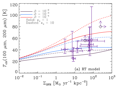
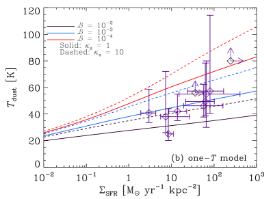
Figure 1: (a) Colour temperature as a function of SFR surface density ($\Sigma_{\mathrm{SFR}}$) in the RT model. The black, blue, and red lines correspond to $\mathcal{D}=10^{-2}$, $10^{-3}$, and $10^{-4}$, respectively. The solid and dashed lines show the results for $\kappa_{\mathrm{s}}=1$ (KS law) and for $\kappa_{\mathrm{s}}=10$ (a burst of star formation), respectively. (b) Dust temperature as a function of $\Sigma_{\mathrm{SFR}}$ in the one-$T$ model. The line species indicate the same meaning as in Panel (a). In both panels, we also display observational data (points with error bars or with arrows for lower/upper limits) summarized in Table 1.

In Fig. 1a, we show the color temperature at 100 and 200 $\micron$ as a function of $\Sigma_{\mathrm{SFR}}$ for the RT model. The colour temperature rises as the SFR surface density increases, although high $\Sigma_{\mathrm{SFR}}$ also indicates high dust surface density (equation 19). This is explained by the following scaling arguments: The KS law indicates that $\Sigma_{\mathrm{dust}}\propto\Sigma_{\mathrm{SFR}}^{1/1.4}$ while the increase of radiation field is proportional to $\Sigma_{\mathrm{SFR}}$. Thus, the increase of radiation field is more significant than that of dust surface density, which means that the dust temperature rises as $\Sigma_{\mathrm{SFR}}$ becomes higher. We also observe that the colour temperature is sensitive to the dust-to-gas ratio, especially at high $\Sigma_{\mathrm{SFR}}$. The rise is steeper for smaller $\mathcal{D}$. The trend of higher dust temperature for lower $\mathcal{D}$ is due to the fact that in a dust poor environment, at fixed $\Sigma_{\mathrm{SFR}}$, the dust is exposed to less shielded UV field, thus being more efficiently heated (see also Sommovigo et al., 2022).

We show the results of the one-$T$ model in Fig. 1b. Recall that the dust temperature is the same as the colour temperature because of the single-temperature assumption. Overall, we find similar dust temperatures to those shown for the RT model. The difference between the two models is much smaller than the variation caused by different dust-to-gas ratios.

We also examine a burst mode of star formation, which is realized by raising $\kappa_{\mathrm{s}}$ (equation 1) in our model. For a burst mode, we examine $\kappa_{\mathrm{s}}=10$, which is inferred for some high-redshift starbursts (e.g. Vallini et al., 2020, 2021; Sommovigo et al., 2021; Ferrara et al., 2022) and is expected from simulations (Pallottini et al., 2022). We observe in Fig. 1 that the dust temperatures are raised by the burst (i.e. higher radiation field). In this sense, raising $\kappa_{\mathrm{s}}$ has a similar effect to decreasing $\mathcal{D}$. This is because of the degeneracy mentioned above (equation 19): The same result is obtained for the same value of $\kappa_{\mathrm{s}}\mathcal{D}^{-1.4}$.

We also plot the observational data (Section 2.4; Table 1) in Fig. 1. We find that the data points favour low $\mathcal{D}$ and/or high $\kappa_{\mathrm{s}}$, although the large error bars make it difficult to obtain a firm constraint on these parameters. If the dust-to-gas ratio is comparable to the value seen in the Milky Way and nearby solar-metallicity galaxies ($\mathcal{D}\sim 0.01$), the dust temperature does not exceed 50 K even with $\kappa_{\mathrm{s}}=10$ at as high $\Sigma_{\mathrm{SFR}}$. Thus, if the dust temperature is higher than $\sim$50 K as observationally indicated for some $z>5$ galaxies it is highly probable that the dust-to-gas ratio is significantly lower than the Milky Way value. It is also interesting to point out that there is a hint of positive correlation between $\Sigma_{\mathrm{SFR}}$ and dust temperature in the observational data although the errors are admittedly large. This positive correlation is consistent with more dust heating radiation in more actively star-forming galaxies.

3.2 Relation between dust mass and dust temperature

Dust surface density has a direct impact on dust temperature through the shielding of stellar radiation. Thus, we expect that it is useful to examine the relation between dust surface density and dust temperature. We show this relation in Fig. 2. Note that we only present $\Sigma_{\mathrm{dust}}$ up to $10^{8}$ M_☉ kpc^-2, beyond which the optically thin assumption for the FIR radiation breaks down (Section 2.2.1). We confirm that the observational sample mostly has $\Sigma_{\mathrm{dust}}<10^{8}$ M_☉ kpc^-2.

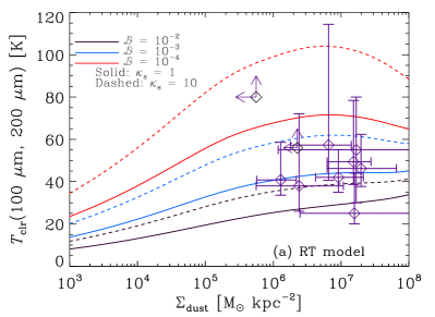
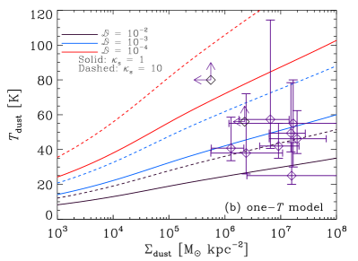
Figure 2: (a) Colour temperature as a function of dust surface density ($\Sigma_{\mathrm{dust}}$) in the RT model. (b) Dust temperature as a function of $\Sigma_{\mathrm{SFR}}$ in the RT model. The line species and data points are the same as in Fig. 1.

In Fig. 2, we observe that the difference in dust temperature among various dust-to-gas ratios and burstiness parameters are clear at all $\Sigma_{\mathrm{dust}}$. This is because, with a fixed value of $\Sigma_{\mathrm{dust}}$, $\Sigma_{\mathrm{SFR}}$ is higher for lower $\mathcal{D}$ (equation 19). A high value of the burstiness parameter ($\kappa_{\mathrm{s}}$) also raises the dust temperature; thus, as noted above, a high burstiness parameter has the same effect as a low $\mathcal{D}$. Both of the RT and one-$T$ models predict similar dust temperatures at $\Sigma_{\mathrm{dust}}\lesssim 10^{7}$ M_☉ kpc^-2. In the RT model, the rise of the dust temperature is saturated at $\Sigma_{\mathrm{dust}}\sim 10^{7}$ M_☉ kpc^-2, beyond which contribution from shielded low-temperature dust to the emission makes the colour temperature lower. In the one-$T$ model, in contrast, the dust temperature rises monotonically even at high $\Sigma_{\mathrm{dust}}$ because of the increase in $\Sigma_{\mathrm{SFR}}$ (equation 19).

We also plot the observational data of the same galaxy sample as above (Table 1) in Fig. 2. As already noted in Section 3.1, lower dust-to-gas ratios or bursty star formation activities are preferred by the data. In particular, the upper left object in this figure (MACS0416_Y1) is likely to be dust-poor with $\mathcal{D}\sim 10^{-4}$ (see also Sommovigo et al., 2022). Since this object hosts an intense star formation activity (as shown by its high $\Sigma_{\mathrm{SFR}}$; Fig. 1) and a low dust abundance, the dust is efficiently heated with little shielding.

Using both Figs. 1 and 2, we could roughly infer the typical dust-to-gas ratio of the sample. We exclude MACS0416_Y1 already discussed above. If the KS law holds for high-redshift galaxies, $\mathcal{D}\lesssim 10^{-4}$ is not accepted because $\Sigma_{\mathrm{SFR}}$ becomes to high to be consistent with the observed SFR surface densities. For example, if $\mathcal{D}=10^{-4}$ and $\Sigma_{\mathrm{dust}}\sim 10^{7}$ M_☉ kpc^-2, where $T_{\mathrm{clr}}$ peaks in Fig. 2a, the gas surface density is $\Sigma_{\mathrm{gas}}\sim 10^{11}$ M_☉ kpc^-2, leading to $\Sigma_{\mathrm{SFR}}\sim 2.5\times 10^{3}$ M_☉ kpc^-2 from the KS law (equation 1). This high value is beyond the range of observed SFR surface densities (Fig. 1), except for MACS0416_Y1. This is why the peak of $T_{\mathrm{clr}}$ does not appear in the range of $\Sigma_{\mathrm{SFR}}$ plotted in Fig. 1. Therefore, the sample (except MACS0416_Y1) should have $\mathcal{D}$ higher than $10^{-4}$ if the KS law holds. On the other hand, a high value of $\mathcal{D}\gtrsim 10^{-2}$ has difficulty in explaining the observed high dust temperatures as argued above. These arguments imply that the dust-to-gas ratios in $z>5$ LBGs are typically significantly lower than $10^{-2}$ but higher than $10^{-4}$; that is, of the order of $\mathcal{D}\sim 10^{-3}$. This value implies a low metallicity: if we use the $\mathcal{D}$–$Z$ relation in nearby galaxies (Rémy-Ruyer et al., 2014), the above value of $\mathcal{D}$ roughly corresponds to $Z\sim 0.2$ Z_☉.

Note that the above results and arguments assumed the KS law, which is poorly confirmed for galaxies at $z\gtrsim 5$. To avoid the conclusions being strongly affected by the assumed KS law, we also examine the relations that do not assume a star formation law in Section 3.3.

3.3 Relations without assuming the KS law

In this subsection, we examine how the surface densities of SFR and dust mass determine the dust temperature without assuming the KS law (without equation 19). That is, we treat $\Sigma_{\mathrm{SFR}}$ and $\Sigma_{\mathrm{dust}}$ as independent parameters. In this case, we do not meed to specify $\mathcal{D}$ or $\kappa_{\mathrm{s}}$.

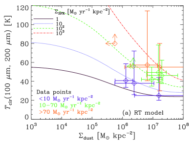
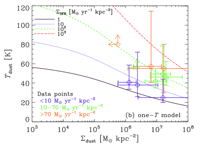
Figure 3: Same diagrams as in Fig. 2 but with fixed values of $\Sigma_{\mathrm{SFR}}$ (i.e. without using the KS law) for the (a) RT and (b) one-$T$ model. The solid, dotted, dashed, and dot–dashed lines present the results for $\Sigma_{\mathrm{SFR}}=1$, 10, $10^{2}$ and $10^{3}$ M_☉ yr^-1 kpc^-2, respectively. The observational data points are the same as in Fig. 2 but are colour-coded according to the SFR surface density ($<10$, 10–70, and $>70$ M_☉ yr^-1 kpc^-2 in blue, green and red, respectively).

In Fig. 3, we show the relation between dust temperature and $\Sigma_{\mathrm{dust}}$ with various $\Sigma_{\mathrm{SFR}}$. The dust temperature becomes lower as the dust surface density increases because of the shielding effect. We observe a large difference in the dust temperature ($\sim 30$–80 K) even at high dust surface density ($\Sigma_{\mathrm{dust}}\sim 10^{7}$ M_☉ kpc^-2) for the range of $\Sigma_{\mathrm{SFR}}$ actually observed for high-redshift galaxies. The range of dust temperature is consistent with the variety in $T_{\mathrm{dust}}$ observed for the galaxies at $z\gtrsim 7$.

We also compare the results with the observational data in Fig. 3. These data are roughly explained by $\Sigma_{\mathrm{SFR}}\sim 1$–$10^{3}$ M_☉ yr^-1 kpc^-2. This range is broadly consistent with the actually observed SFR surface densities (Fig. 1). For comparison, we colour-code the observational data according to the range of $\Sigma_{\mathrm{SFR}}$ ($<10$, 10–70, and $>70$ M_☉ yr^-1 kpc^-2, in blue, green, and orange, respectively). The blue-green-orange trend in the observational data is indeed consistent with the tendency of theoretical predictions with rising $\Sigma_{\mathrm{SFR}}$ (also shown by blue, green and orange lines). Although the large error bars hinder drawing a firm conclusion, the overall consistency in the $T_{\mathrm{dust}}$–$\Sigma_{\mathrm{dust}}$–$\Sigma_{\mathrm{SFR}}$ relation indicates the success of our models.

Comparing the two panels in Fig. 3, we find that the two (RT and one-$T$) models are similar. The largest difference between the two models appears at high dust surface density as also found in Fig. 2: In the one-$T$ model, all dust has a single temperature, which monotonically drops as the dust mass increases. In the RT model, in contrast, the drop of dust temperature is saturated at high $\Sigma_{\mathrm{dust}}$ and low $\Sigma_{\mathrm{SFR}}$ because the shielded portion of dust has too low a temperature to contribute significantly to the luminosity at $\lambda\leq 200~{}\micron$. It is reminded here that the CMB heating, which we neglected (Section 2), should be included if we are interested in the temperature drop at high $\Sigma_{\mathrm{dust}}$. In particular, for the one-$T$ model, the dust temperature would not continue to drop below the CMB temperature towards high $\Sigma_{\mathrm{dust}}$.

The result shown in Fig. 3 also indicates that, if we obtain two of the three quantities ($T_{\mathrm{dust}}$, $\Sigma_{\mathrm{dust}}$, and $\Sigma_{\mathrm{SFR}}$), we can estimate the other using our model. An interesting application would be to obtain $T_{\mathrm{dust}}$ from $\Sigma_{\mathrm{dust}}$ and $\Sigma_{\mathrm{SFR}}$, both of which could be estimated from rest-frame UV data as well (through the UV spectral index and the UV luminosity; see section 2 of Ferrara et al. 2017). Ferrara et al. (2022) estimated the dust temperature basically in this way. Another application would be to derive $\Sigma_{\mathrm{SFR}}$ from $T_{\mathrm{dust}}$ and $\Sigma_{\mathrm{dust}}$. If the obtained $\Sigma_{\mathrm{SFR}}$ is converted to $\Sigma_{\mathrm{gas}}$ using the KS law, we could estimate the dust-to-gas ratio ($\Sigma_{\mathrm{dust}}/\Sigma_{\mathrm{gas}}$). We already constrained the dust-to-gas ratio in this way in Section 3.2, and argued that the typical dust-to-gas ratio is of the order of $\sim 10^{-3}$.

4 Discussion

4.1 Radiative transfer and one-$T$ models

In the above, we have shown that the RT and one-$T$ models overall predict similar dust temperatures. However, the difference between the two models appears at $\Sigma_{\mathrm{dust}}\gtrsim 10^{7}$ M_☉ kpc^-2, where the RT model shows a saturation or decrease of the dust temperature (colour temperature) because of shielding (Fig. 2; Section 3.2). In the one-$T$ model, in contrast, the dust temperature always continues to increase even if the dust surface density increases beyond $\Sigma_{\mathrm{dust}}\sim 10^{7}$ M_☉ kpc^-2. Thus, the dust–stars distribution geometry, which affects shielding of dust-heating radiation, has a significant impact on the dust temperature at $\Sigma_{\mathrm{dust}}\gtrsim 10^{7}$ M_☉ kpc^-2. This in turn means that the geometry of dust and star distributions only has a minor influence on the dust temperature at lower dust surface densities.

From the above results, we expect that the SED shapes of dust emission are different between the two (RT and one-$T$) models at high dust surface densities. To visualize this expectation, we present in Fig. 4 the SEDs for various $\Sigma_{\mathrm{dust}}$ with a fixed $\Sigma_{\mathrm{gas}}$ (so a fixed $\Sigma_{\mathrm{SFR}}$, whose value is determined by the KS law). We choose the case of $\Sigma_{\mathrm{SFR}}=30$ M_☉ yr^-1 kpc^-2 ($\Sigma_{\mathrm{gas}}\simeq 4.2\times 10^{9}$ M_☉ kpc^-2), which is roughly in the middle of the observational sample we adopted (Fig. 1). We examine $\Sigma_{\mathrm{dust}}=4.2\times 10^{5}$, $4.2\times 10^{6}$, and $4.2\times 10^{7}$ M_☉ kpc^-2, which correspond to $\mathcal{D}=10^{-4}$, $10^{-3}$, and $10^{-2}$, respectively.

Note that, in reality, the emission at wavelengths well below the SED peak position is not precisely predicted in our model, since stochastically heated very small grains (e.g. Draine & Anderson, 1985), which are not included in our model, contribute to the emission significantly. Moreover, complex dust–stars geometries on small spatial scales, which are not included in our models (see Section 4.3) would also lead to hot dust components located in the vicinity of compact, actively star-forming regions. Such hot dust components contribute to emission at short wavelengths (Sommovigo et al., 2020), which is missing in our prediction. Such compact region could enhance the optical depth, and possibly make the region optically thick for short-wavelength dust emission. Thus, we do not discuss the difference in SED shape on the Wien side, but focus on the wavelengths around the SED peak and on the Rayleigh–Jeans side.

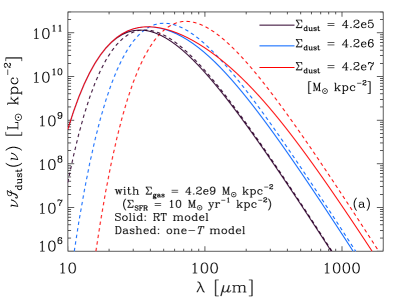
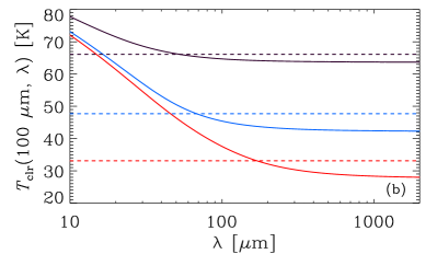
Figure 4: (a) Dust emission SEDs for $\Sigma_{\mathrm{gas}}=4.2\times 10^{9}$ M_☉ kpc^-2 (corresponding to $\Sigma_{\mathrm{SFR}}=10$ M_☉ yr^-1 kpc^-2 in the KS law). In order to examine the effect of dust optical depth (dust surface density) on the SED, we show the results with various dust-to-gas ratios, $\Sigma_{\mathrm{dust}}=4.2\times 10^{5}$, $4.2\times 10^{6}$, and $4.2\times 10^{7}$ M_☉ kpc^-2 (black, blue and red lines, respectively), corresponding to $\mathcal{D}=10^{-4}$, $10^{-3}$, and $10^{-2}$, respectively, in the RT model (solid lines) and the one-$T$ model (dashed lines). The vertical axis shows $\Sigma_{\mathrm{lum,dust}}^{i}(\nu)$ ($i=\mathrm{RT}$ or one-$T$ depending on the model) multiplied by the frequency. (b) Colour temperature as a function of wavelength for the RT model (solid lines). One of the wavelengths is fixed to 100 $\micron$, and the other is moved freely. For comparison, we also show the dust temperature in the one-$T$ model (dashed lines). Each colour corresponds to the same value of $\Sigma_{\mathrm{dust}}$ as in Panel (a).

We observe in Fig. 4 that the two (RT and one-$T$) models show different trends with increasing $\Sigma_{\mathrm{dust}}$. In the RT model, the SED extends to longer wavelengths as the dust abundance becomes larger with the luminosity at the shortest wavelengths fixed. This is because cold layers of dust are added if we increase $\Sigma_{\mathrm{dust}}$ with a fixed value of $\Sigma_{\mathrm{SFR}}$ (i.e. a fixed stellar luminosity). In contrast, in the one-$T$ model, the SED shifts towards longer wavelengths as $\Sigma_{\mathrm{dust}}$ increases, reflecting the drop of dust temperature. This is because the stellar radiation received per dust mass decreases as the dust increases. In both models, we see a slight rise of the SED peak with $\Sigma_{\mathrm{dust}}$ simply because of the increase in the energy absorbed by dust. At low $\Sigma_{\mathrm{dust}}$, the difference between the two models is small. This means that the dust temperature is well approximated with a single value in the RT model because shielding is weak. In contrast, at high $\Sigma_{\mathrm{dust}}$, the SEDs are different between the two models. Therefore, if the dust surface density is as high as $\Sigma_{\mathrm{dust}}\gtrsim 10^{7}$ M_☉ kpc^-2, detailed dust temperature structures created by RT effects are important in the detailed SED shape.

From the difference in SED shape between the two models, we expect that the colour temperature in the RT model depends on the selected wavelengths at high $\Sigma_{\mathrm{dust}}$. In Fig. 4b, we show the colour temperature as a function of wavelength. We fix one of the wavelengths to 100 $\micron$ and move the other freely, and present $T_{\mathrm{clr}}(100~{}\micron,\,\lambda)$. We observe that the colour temperature monotonically decreases as $\lambda$ increases because we selectively observe lower-temperature dust at longer wavelengths. If we focus on long (rest-frame) wavelengths ($\lambda\gtrsim 100~{}\micron$), which are often used by ALMA observations (Bands 6–8) of high-redshift galaxies, the colour temperature is not sensitive to the selected wavelengths. When we use Band 9 (450 $\micron$) for galaxies at $z\gtrsim 7$ (i.e. $\lambda\lesssim 60~{}\micron$), the colour temperature is systematically high in the RT model since high-temperature layers dominate the emission at such a short wavelength. Thus, dust temperature estimates including Band 9 need to be carefully interpreted by noting a possibility of multi-$T_{\mathrm{dust}}$ structures. At long wavelengths, such a multi-temperature effect is not important; indeed, the colour temperature is almost constant at $\lambda\gtrsim 200~{}\micron$, and is similar to the dust temperature in the one-$T$ model. Thus, the above predictions on the colour temperature are not altered significantly as long as we focus on ALMA Bands 6–8. If we include a Band 9 observation in the SED analysis, it is safer to include multiple bands from Bands 6–8 as well in order to examine the multi-$T_{\mathrm{dust}}$ effect on the SED.

4.2 Effects of dust properties

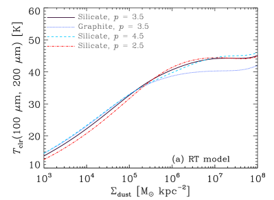
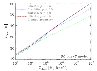
Figure 5: Dust temperature as a function of dust surface density in the (a) RT and (b) one-$T$ models for a variety of dust properties. We adopt $\mathcal{D}=10^{-3}$ and $\kappa_{\mathrm{s}}=1$. The solid, dashed, and dot–dashed lines correspond to silicate with $p=3.5$ (MRN), 4.5, and 2.5, respectively. The dotted line shows graphite with $p=3.5$. The homogeneous geometry is adopted for the one-$T$ model. In Panel (b), we also show the result of the clumpy geometry with $\xi_{\mathrm{cl}}=3$ for silicate with $p=3.5$ (triple-dot–dashed line) in addition to the honogeneous geometry.

We examine the variation of dust properties. We vary the dust composition and the grain size distribution (Section 2.1.2). We fix $\mathcal{D}=10^{-3}$. We show the relation between dust temperature and $\Sigma_{\mathrm{dust}}$ for silicate and graphite with $p=3.5$, and for $p=2.5$ and 4.5 with silicate in Fig. 5. The burstiness parameter is fixed to $\kappa_{\mathrm{s}}=1$.

We observe in Fig. 5 that the dust temperature is insensitive to $p$ in both RT and one-$T$ models. While large $p$ indicates more efficient absorption of UV radiation (because of more small grains), it also means more efficient shielding. These two effects counteract each other. The difference between silicate and graphite is more apparent, especially at high $\Sigma_{\mathrm{dust}}$. This is not only due to more efficient shielding, but also because of more efficient emission (higher mass absorption coefficient) for graphite. More efficient emission leads to a lower equilibrium dust temperature. Comparing the RT and one-$T$ models, we confirm significant difference at high $\Sigma_{\mathrm{dust}}$ as pointed out above. In both models, graphite predicts lower dust temperatures than silicate at dust surface densities ($\sim 10^{7}$ M_☉ kpc^-2) appropriate for the $z>7$ sample above but the difference is only $\sim 10$ per cent.

In the one-$T$ model (Fig. 5b), we also show the clumpy geometry with $\xi_{\mathrm{cl}}=3$ (for silicate with $p=3.5$), which shows significantly lower dust temperature than the homogensous geometry at high $\Sigma_{\mathrm{dust}}$. This is because, as explained in Section 2.2.2, dust only covers the galaxy surface with a fraction of $1/\xi_{\mathrm{cl}}$. This means that dust can only absorb a part of stellar light even if the dust abundance is high. Since the total emission energy of dust is scaled with $T_{\mathrm{dust}}^{4+\beta}$, we obtain a scaling of $T_{\mathrm{dust}}\propto\xi_{\mathrm{cl}}^{-1/(4+\beta)}$ ($\xi_{\mathrm{cl}}>1$) at high dust surface density. This scaling is useful to infer the dust temperature with different values of $\xi_{\mathrm{cl}}>1$ (recall again that the result is similar to the homogensous case with $\xi_{\mathrm{cl}}\lesssim 1$) at high dust surface densities. At low dust surface densities, the dust is optically thin for UV radiation; in this case, the total radiation energy absorbed by dust is determined by the total dust mass, and is not sensitive to dust distribution geometry. Thus, clumpy geometry gives a conservative (low) dust temperature, which means that the requirement for low $\mathcal{D}$ or higher $\kappa_{\mathrm{s}}$ is pronounced if we aim at explaining the high dust temperatures with clumpy geometry compared with the uniform geometry.

4.3 Further complexities

Although the geometries of dust–stars distribution in real galaxies are complex, we still expect that our theory based on the surface densities are applicable to a variety of galaxies. This is because the radiation field is also a ‘surface’ quantity in the sense that it has the same physical dimension as the surface luminosity (Section 2.1.1). Our predictions are further checked with observations of nearby galaxies (Chiang et al., in preparation). Numerical simulations with more complex dust–stars geometries could also be used to examine the robustness of our predictions.

However, the effect of local intense radiation sources may not be included in our simple treatment. Some analytic and numerical studies showed that a dust component concentrated nearby an intensely star-forming region could have a large contribution to the FIR luminosity of the galaxy (Behrens et al., 2018; Sommovigo et al., 2020; Pallottini et al., 2022). Complex dust–stars geometries are also shown observationally for galaxies at $z\sim 7$ (Willott et al., 2015; Bowler et al., 2022). Therefore, our simple analytic treatments should be carefully applied to real high-redshift galaxies, and studies focusing on small-scale structures should supplement our understanding of what regulates the dust temperature in high-redshift galaxies. Interestingly, the necessity of low dust abundance in explaining the high dust temperature is common between our work and some studies that included small-scale or complicated geometries (Liang et al., 2019; Ma et al., 2019; Sommovigo et al., 2022).

5 Conclusions

For the purpose of interpreting observed dust temperatures at high redshift ($z>5$), we construct analytic models to calculate the dust temperature under given star formation activity and dust properties (especially dust abundance). The models are described by the surface densities of gas mass and SFR since the surface quantities are important to describe the radiation field intensity and the dust optical depth. We develop the following two models that can be treated analytically: (i) RT and (ii) one-$T$ models. In the first model, we consider the multi-temperature (or dust shielding) effect within the framework of plane-parallel treatment by putting the stars in the midplane of the disc and the dust in the screen geometry. The dust temperature in this model is defined by the colour temperature at two selected wavelengths (100 and 200 $\micron$ by default). In the second model, we consider an opposite extreme by considering that dust and stars are well mixed, so that the dust is assumed to have a single temperature. In this model, the dust temperature is determined by the global balance between the absorbed and radiated energy by the dust. These two extremes serve to bracket the most realistic scenario.

We particularly focus on the dust temperature as a function of SFR surface density ($\Sigma_{\mathrm{SFR}}$) and dust surface density ($\Sigma_{\mathrm{dust}}$). As expected, the dust temperature rises with increasing $\Sigma_{\mathrm{SFR}}$ and $\Sigma_{\mathrm{dust}}$ (which has a positive relation with $\Sigma_{\mathrm{SFR}}$ because of the KS law). However, these relations depend on the dust-to-gas ratio ($\mathcal{D}$), since it affects the relation between $\Sigma_{\mathrm{SFR}}$ and $\Sigma_{\mathrm{dust}}$ (equation 19). Lower values of $\mathcal{D}$ predicts higher dust temperatures. Thus, low dust abundance ($\lesssim 10^{-3}$) can be a reason for observed high dust temperatures ($T_{\mathrm{dust}}\gtrsim 40$ K) in high-redshift galaxies. Another reason could be a burst of star formation (i.e. high $\kappa_{\mathrm{s}}$). The grain size distribution and the dust composition have less impacts on the dust temperature than $\mathcal{D}$ and $\kappa_{\mathrm{s}}$.

The RT and one-$T$ models predict similar dust temperatures except at high dust surface density ($\Sigma_{\mathrm{dust}}>10^{7}$ M_☉ kpc^-2). Some ALMA-detected galaxies at $z>5$ may be located in this high-$\Sigma_{\mathrm{dust}}$ regime, which means that a careful radiative transfer treatment is necessary to predict precise dust temperature. However, the difference among different values of $\mathcal{D}$ and $\kappa_{\mathrm{s}}$ is significant, and the conclusion that high-redshift LBGs favour low $\mathcal{D}\lesssim 10^{-3}$ (if $\kappa_{\mathrm{s}}\lesssim 10$) is not altered.

We also examine the relation between dust temperature and $\Sigma_{\mathrm{dust}}$ without assuming the KS law; that is, we treat $\Sigma_{\mathrm{SFR}}$ as an independent parameter. Overall, higher $\Sigma_{\mathrm{SFR}}$ indicates higher dust temperature and we predict $T_{\mathrm{dust}}\sim 30$–80 K for the range of $\Sigma_{\mathrm{SFR}}$ and $\Sigma_{\mathrm{dust}}$ appropriate for high-redshift ($z>5$) LBGs. The observational data ($\Sigma_{\mathrm{SFR}}$, $\Sigma_{\mathrm{dust}}$, and $T_{\mathrm{dust}}$) of $z>5$ LBGs are consistent with the calculation results. Interestingly, we also find a trend that LBGs with higher $\Sigma_{\mathrm{SFR}}$ and lower $\Sigma_{\mathrm{dust}}$ tend to have higher $T_{\mathrm{dust}}$, which is consistent with our prediction (Fig. 3).

The difference between the two (RT and one-$T$) models is further examined. We observe a significant difference in SED shape between the two models at $\Sigma_{\mathrm{dust}}\gtrsim 10^{7}$ M_☉ kpc^-2 since the superposition of layers with various dust temperatures is important at such a high dust surface density in the RT model. Thus, if the dust surface density is higher than $\sim 10^{7}$ M_☉ kpc^-2, a detailed radiative transfer calculation is necessary to discuss the detailed shape of dust emission SED. We, however, find that, in the range of dust surface density appropriate for high-redshift LBGs, the colour temperature in the RT model is similar to the dust temperature in the one-$T$ model as long as we use $\lambda\sim 100$–200 $\micron$. Thus, the dust temperature measured in ALMA Bands 6–8 ($\sim 650$–1,200 $\micron$) for $z\gtrsim 5$ galaxies is not sensitive to the detailed radiative transfer effects. Note that Band 9 ($\sim 450~{}\micron$) may selectively observe high-dust-temperature layers at $\Sigma_{\mathrm{dust}}\gtrsim 10^{7}$ M_☉ kpc^-2, if the multi-$T_{\mathrm{dust}}$ structure is as significant as realized in the RT model.

In the one-$T$ model, we also investigate the effect of clumpiness in dust distribution geometry. We only consider the case where the density contrast between the clumps and the diffuse medium is large since otherwise the resulting dust temperature is similar to the homogeneous geometry. At low $\Sigma_{\mathrm{dust}}$, the clumpy geometry predicts almost the same dust temperature as the homogeneous geometry. However, at high $\Sigma_{\mathrm{dust}}\gtrsim 10^{7}$ M_☉ kpc^-2, the dust temperature is lower in the clumpy case because the dust effectively covers only a certain fraction of the galaxy surface. This strengthens the requirement of low dust-to-gas ratio and/or high $\kappa_{\mathrm{s}}$ to achieve a high dust temperature.

From the above, we conclude that the high dust temperatures ($T_{\mathrm{dust}}\gtrsim 40$ K) in some ALMA-detected $z\gtrsim 7$ galaxies is caused by a low dust-to-gas ratio ($\mathcal{D}\lesssim 10^{-3}$) if the KS law holds in high-redshift galaxies. A burst-like star formation with $\kappa_{\mathrm{s}}\gtrsim 10$ could give another explanation for the high dust temperatures. These conclusions are not sensitive to the dust properties (dust composition and grain size distribution) and detailed radiative transfer effect. In the companion paper (Chiang et al., in preparation), we test our model using spatially resolved observations of nearby star-forming galaxies.

Data Availability

Data related to this publication and its figures are available on request from the corresponding author.

References

- Abdurro’uf et al. (2021) Abdurro’uf Lin Y.-T., Wu P.-F., Akiyama M., 2021, ApJS, 254, 15
- Aoyama et al. (2019) Aoyama S., et al., 2019, MNRAS, 484, 1852
- Bakx et al. (2020) Bakx T. J. L. C., et al., 2020, MNRAS, 493, 4294
- Bakx et al. (2021) Bakx T. J. L. C., et al., 2021, MNRAS, 508, L58
- Behrens et al. (2018) Behrens C., Pallottini A., Ferrara A., Gallerani S., Vallini L., 2018, MNRAS, 477, 552
- Béthermin et al. (2015) Béthermin M., et al., 2015, A&A, 573, A113
- Béthermin et al. (2020) Béthermin M., et al., 2020, A&A, 643, A2
- Bohren & Huffman (1983) Bohren C. F., Huffman D. R., 1983, Absorption and Scattering of Light by Small Particles. Wiley, New York
- Boquien et al. (2019) Boquien M., Burgarella D., Roehlly Y., Buat V., Ciesla L., Corre D., Inoue A. K., Salas H., 2019, A&A, 622, A103
- Bouwens et al. (2016) Bouwens R. J., et al., 2016, ApJ, 833, 72
- Bouwens et al. (2020) Bouwens R., et al., 2020, ApJ, 902, 112
- Bowler et al. (2022) Bowler R. A. A., Cullen F., McLure R. J., Dunlop J. S., Avison A., 2022, MNRAS, 510, 5088
- Buat & Xu (1996) Buat V., Xu C., 1996, A&A, 306, 61
- Burgarella et al. (2020) Burgarella D., Nanni A., Hirashita H., Theulé P., Inoue A. K., Takeuchi T. T., 2020, A&A, 637, A32
- Burgarella et al. (2022) Burgarella D., et al., 2022, arXiv e-prints, p. arXiv:2203.02059
- Calzetti et al. (2000) Calzetti D., Armus L., Bohlin R. C., Kinney A. L., Koornneef J., Storchi-Bergmann T., 2000, ApJ, 533, 682
- Capak et al. (2015) Capak P. L., et al., 2015, Nature, 522, 455
- Cazaux & Tielens (2004) Cazaux S., Tielens A. G. G. M., 2004, ApJ, 604, 222
- Chen et al. (2018) Chen L.-H., Hirashita H., Hou K.-C., Aoyama S., Shimizu I., Nagamine K., 2018, MNRAS, 474, 1545
- Chen et al. (2021) Chen Y. Y., Hirashita H., Wang W.-H., Nakai N., 2021, MNRAS,
- da Cunha et al. (2008) da Cunha E., Charlot S., Elbaz D., 2008, MNRAS, 388, 1595
- da Cunha et al. (2013) da Cunha E., et al., 2013, ApJ, 766, 13
- Dayal & Ferrara (2018) Dayal P., Ferrara A., 2018, Phys. Rep., 780, 1
- Di Mascia et al. (2021) Di Mascia F., Gallerani S., Ferrara A., Pallottini A., Maiolino R., Carniani S., D’Odorico V., 2021, MNRAS, 506, 3946
- Draine & Anderson (1985) Draine B. T., Anderson N., 1985, ApJ, 292, 494
- Draine & Li (2007) Draine B. T., Li A., 2007, ApJ, 657, 810
- Faisst et al. (2017) Faisst A. L., et al., 2017, ApJ, 847, 21
- Faisst et al. (2020) Faisst A. L., Fudamoto Y., Oesch P. A., Scoville N., Riechers D. A., Pavesi R., Capak P., 2020, MNRAS, 498, 4192
- Ferrara et al. (2017) Ferrara A., Hirashita H., Ouchi M., Fujimoto S., 2017, MNRAS, 471, 5018
- Ferrara et al. (2019) Ferrara A., Vallini L., Pallottini A., Gallerani S., Carniani S., Kohandel M., Decataldo D., Behrens C., 2019, MNRAS, 489, 1
- Ferrara et al. (2022) Ferrara A., et al., 2022, MNRAS, 512, 58
- Fudamoto et al. (2020) Fudamoto Y., et al., 2020, A&A, 643, A4
- Fudamoto et al. (2021) Fudamoto Y., et al., 2021, Nature, 597, 489
- Fudamoto et al. (2022) Fudamoto Y., Inoue A. K., Sugahara Y., 2022, MNRAS, submitted (arXiv:2206.01879)
- Gould & Salpeter (1963) Gould R. J., Salpeter E. E., 1963, ApJ, 138, 393
- Harikane et al. (2020) Harikane Y., et al., 2020, ApJ, 896, 93
- Hashimoto et al. (2019) Hashimoto T., et al., 2019, PASJ, 71, 71
- Hirashita & Ferrara (2002) Hirashita H., Ferrara A., 2002, MNRAS, 337, 921
- Hirashita & Inoue (2019) Hirashita H., Inoue A. K., 2019, MNRAS, 487, 961
- Hirashita & Kobayashi (2013) Hirashita H., Kobayashi H., 2013, Earth, Planets, and Space, 65, 1083
- Hirashita et al. (2003) Hirashita H., Buat V., Inoue A. K., 2003, A&A, 410, 83
- Hirashita et al. (2014) Hirashita H., Ferrara A., Dayal P., Ouchi M., 2014, MNRAS, 443, 1704
- Hirashita et al. (2015) Hirashita H., Nozawa T., Villaume A., Srinivasan S., 2015, MNRAS, 454, 1620
- Inami et al. (2022) Inami H., et al., 2022, arXiv e-prints, p. arXiv:2203.15136
- Inoue et al. (2000) Inoue A. K., Hirashita H., Kamaya H., 2000, PASJ, 52, 539
- Inoue et al. (2020) Inoue A. K., Hashimoto T., Chihara H., Koike C., 2020, MNRAS, 495, 1577
- Kennicutt (1998a) Kennicutt Jr. R. C., 1998a, ARA&A, 36, 189
- Kennicutt (1998b) Kennicutt Jr. R. C., 1998b, ApJ, 498, 541
- Knudsen et al. (2017) Knudsen K. K., Watson D., Frayer D., Christensen L., Gallazzi A., Michałowski M. J., Richard J., Zavala J., 2017, MNRAS, 466, 138
- Kroupa (2002) Kroupa P., 2002, Science, 295, 82
- Kruegel (2003) Kruegel E., 2003, The physics of interstellar dust. IoP Publishing, Bristol
- Laporte et al. (2017) Laporte N., et al., 2017, ApJ, 837, L21
- Laporte et al. (2019) Laporte N., et al., 2019, MNRAS, 487, L81
- Leitherer et al. (1999) Leitherer C., et al., 1999, ApJS, 123, 3
- Liang et al. (2019) Liang L., et al., 2019, MNRAS, 489, 1397
- Lim et al. (2020) Lim C.-F., et al., 2020, ApJ, 889, 80
- Liu & Hirashita (2019) Liu H.-M., Hirashita H., 2019, MNRAS, 490, 540
- Ma et al. (2019) Ma X., et al., 2019, MNRAS, 487, 1844
- Magnelli et al. (2014) Magnelli B., et al., 2014, A&A, 561, A86
- Mathis et al. (1977) Mathis J. S., Rumpl W., Nordsieck K. H., 1977, ApJ, 217, 425
- Nanni et al. (2020) Nanni A., Burgarella D., Theulé P., Côté B., Hirashita H., 2020, A&A, 641, A168
- Omukai et al. (2005) Omukai K., Tsuribe T., Schneider R., Ferrara A., 2005, ApJ, 626, 627
- Osterbrock (2006) Osterbrock D. E., 2006, Astrophysics of gaseous nebulae and active galactic nuclei, 2nd edn. Sausalito, CA
- Pallottini et al. (2022) Pallottini A., et al., 2022, MNRAS, 513, 5621
- Rémy-Ruyer et al. (2014) Rémy-Ruyer A., et al., 2014, A&A, 563, A31
- Romano et al. (2022) Romano L. E. C., Nagamine K., Hirashita H., 2022, MNRAS, 514, 1461
- Schneider et al. (2006) Schneider R., Omukai K., Inoue A. K., Ferrara A., 2006, MNRAS, 369, 1437
- Schouws et al. (2022) Schouws S., et al., 2022, ApJ, 928, 31
- Schreiber et al. (2018) Schreiber C., Elbaz D., Pannella M., Ciesla L., Wang T., Franco M., 2018, A&A, 609, A30
- Silva et al. (1998) Silva L., Granato G. L., Bressan A., Danese L., 1998, ApJ, 509, 103
- Sommovigo et al. (2020) Sommovigo L., Ferrara A., Pallottini A., Carniani S., Gallerani S., Decataldo D., 2020, MNRAS, 497, 956
- Sommovigo et al. (2021) Sommovigo L., Ferrara A., Carniani S., Zanella A., Pallottini A., Gallerani S., Vallini L., 2021, MNRAS, 503, 4878
- Sommovigo et al. (2022) Sommovigo L., et al., 2022, MNRAS, 513, 3122
- Sugahara et al. (2021) Sugahara Y., et al., 2021, ApJ, 923, 5
- Takagi et al. (2003) Takagi T., Vansevicius V., Arimoto N., 2003, PASJ, 55, 385
- Takeuchi et al. (2005) Takeuchi T. T., Ishii T. T., Nozawa T., Kozasa T., Hirashita H., 2005, MNRAS, 362, 592
- Tamura et al. (2019) Tamura Y., et al., 2019, ApJ, 874, 27
- Tielens (2005) Tielens A. G. G. M., 2005, The Physics and Chemistry of the Interstellar Medium. Cambridge University Press, Cambridge
- Vallini et al. (2020) Vallini L., Ferrara A., Pallottini A., Carniani S., Gallerani S., 2020, MNRAS, 495, L22
- Vallini et al. (2021) Vallini L., Ferrara A., Pallottini A., Carniani S., Gallerani S., 2021, MNRAS, 505, 5543
- Városi & Dwek (1999) Városi F., Dwek E., 1999, ApJ, 523, 265
- Viero et al. (2022) Viero M. P., Sun G., Chung D. T., Moncelsi L., Condon S. S., 2022, MNRAS, in press (arXiv:2203.14312)
- Vijayan et al. (2022) Vijayan A. P., et al., 2022, MNRAS, 511, 4999
- Watson et al. (2015) Watson D., Christensen L., Knudsen K. K., Richard J., Gallazzi A., Michałowski M. J., 2015, Nature, 519, 327
- Weingartner & Draine (2001) Weingartner J. C., Draine B. T., 2001, ApJ, 548, 296
- Willott et al. (2015) Willott C. J., Carilli C. L., Wagg J., Wang R., 2015, ApJ, 807, 180
- Yajima et al. (2014) Yajima H., Nagamine K., Thompson R., Choi J.-H., 2014, MNRAS, 439, 3073
- Yamasawa et al. (2011) Yamasawa D., Habe A., Kozasa T., Nozawa T., Hirashita H., Umeda H., Nomoto K., 2011, ApJ, 735, 44