Automating DBSCAN via Deep Reinforcement Learning

Abstract.

DBSCAN is widely used in many scientific and engineering fields because of its simplicity and practicality. However, due to its high sensitivity parameters, the accuracy of the clustering result depends heavily on practical experience. In this paper, we first propose a novel Deep Reinforcement Learning guided automatic DBSCAN parameters search framework, namely DRL-DBSCAN. The framework models the process of adjusting the parameter search direction by perceiving the clustering environment as a Markov decision process, which aims to find the best clustering parameters without manual assistance. DRL-DBSCAN learns the optimal clustering parameter search policy for different feature distributions via interacting with the clusters, using a weakly-supervised reward training policy network. In addition, we also present a recursive search mechanism driven by the scale of the data to efficiently and controllably process large parameter spaces. Extensive experiments are conducted on five artificial and real-world datasets based on the proposed four working modes. The results of offline and online tasks show that the DRL-DBSCAN not only consistently improves DBSCAN clustering accuracy by up to $26\%$ and $25\%$ respectively, but also can stably find the dominant parameters with high computational efficiency. The code is available at GitHub.

1. INTRODUCTION

Density-Based Spatial Clustering of Applications with Noise (DBSCAN) (Ester et al., 1996) is a typical density based clustering method that determines the cluster structure according to the tightness of the sample distribution. It automatically determines the number of final clusters according to the nature of the data, has low sensitivity to abnormal points, and is compatible with any cluster shape. In terms of application areas, benefiting from its strong adaptability to datasets of unknown distribution, DBSCAN is the preferred solution for many clustering problems, and has achieved robust performance in fields such as financial analysis (Huang et al., 2019; Yang et al., 2014), commercial research (Fan et al., 2021; Wei et al., 2019), urban planning (Li and Li, 2007; Pavlis et al., 2018), seismic research (Fan and Xu, 2019; Kazemi-Beydokhti et al., 2017; Vijay and Nanda, 2019), recommender system (Guan et al., 2018; Kużelewska and Wichowski, 2015), genetic engineering (Francis et al., 2011; Mohammed et al., 2018), etc.

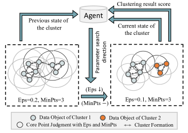
Figure 1. Markov process of parameter search. The agent uses the data as the environment, and determines the action to search by observing the clustering state and reward.

However, the two global parameters of DBSCAN, the distance of the cluster formation $Eps$ and the minimum data objects required inside the cluster $MinPts$, that need to be manually specified, bring Three challenges to its clustering process. First, parameters free challenge. $Eps$ and $MinPts$ have considerable influence on the clustering effect, but it needs to be determined a priori. The method based on the $k$-distance (Liu et al., 2007; Mitra and Nandy, 2011) estimates the possible values of the $Eps$ through significant changes in the curve, but it still needs to manually formulate $Minpts$ parameters in advance. Although some improved DBSCAN methods avoid the simultaneous adjustment of $Eps$ and $MinPts$ to varying degrees, but they also necessary to pre-determine the cutoff distance parameter (Diao et al., 2018), grid parameter (Darong and Peng, 2012), Gaussian distribution parameter (Smiti and Elouedi, 2012) or fixed $Minpts$ parameter (Hou et al., 2016; Akbari and Unland, 2016). Therefore, the first challenge is how to perform DBSCAN clustering without tuning parameters based on expert knowledge. Second, adaptive policy challenge. Due to the different data distributions and cluster characteristics in clustering tasks, traditional DBSCAN parameter searching methods based on fixed patterns (Liu et al., 2007; Mitra and Nandy, 2011) encounter bottlenecks in the face of unconventional data problems. Moreover, hyperparameter optimization methods (Karami and Johansson, 2014; Bergstra et al., 2011; Lessmann et al., 2005) using external clustering evaluation index based on label information as objective functions are not effective in the absence of data label information. The methods (Lai et al., 2019; Zhou and Gao, 2014) that only use the internal clustering evaluation index as the objective function, are limited by the accuracy problem, despite that they do not require label information. In addition, for streaming data that needs to be clustered continuously but the data distribution is constantly changing, the existing DBSCAN parametric search methods do not focus on how to use past experience to adaptively formulate search policies for newly arrived data. Thus, how to effectively and adaptively adjust the parameter search policy of the data and be compatible with the lack of label information is regarded as the second challenge. Third, computational complexity challenge. Furthermore, the parameter search is limited by the parameter space that cannot be estimated. Searching too many invalid parameters will increase the search cost (Kanervisto et al., 2020), and too large search space will bring noise interfering with clustering accuracy (Dulac-Arnold et al., 2015). Hence, how to quickly search for the optimal parameters while securing clustering accuracy is the third challenge that needs to be addressed.

In recent years, Deep Reinforcement Learning (DRL) (Fujimoto et al., 2018; Lillicrap et al., 2015) has been widely used for tasks lacking training data due to its ability to learn by receiving feedback from the environment (Peng et al., 2022). In this paper, to handle the problem of missing optimal DBSCAN parameter labeling and the challenges above, we propose DRL-DBSCAN, a novel, adaptive, recursive Deep Reinforcement Learning DBSCAN parameter search framework, to obtain optimal parameters in multiple scenarios and tasks stably. We first take the cluster changes after each step of clustering as the observable state, the parameter adjustment direction as the action, and transform the parameter search process into a Markov decision process in which the DRL agents autonomously perceive the environment to make decisions (Fig. 1). Then, through weak supervision, we construct reward based on a small number of external clustering indices, and fuse the global state and the local states of multiple clusters based on the attention mechanism, to prompt the agents to learn how to adaptively perform the parameter search for different data. In addition, to improve the learning efficiency of the policy network, we optimize the base framework through a recursive mechanism based on agents with different search precisions to achieve the highest clustering accuracy of the parameters stably and controllable. Finally, considering the existence of DBSCAN clustering scenarios with no labels, few labels, initial data, and incremental data, we designed four working modes: retraining mode, continuous training mode, pre-training test mode, and maintenance test mode for compatibility. We extensively evaluate the parameter search performance of DRL-DBSCAN with four modes for the offline and online tasks on the public Pathbased, Compound, Aggregation, D31 and Sensor datasets. The results show that DRL-DBSCAN can break away from manually defined parameters, automatically and efficiently discover suitable DBSCAN clustering parameters, and has stability in multiple downstream tasks.

The contributions of this paper are summarized as follows: (1) The first DBSCAN parameter search framework guided by DRL is proposed to automatically select the parameter search directions. (2) A weakly-supervised reward mechanism and a local cluster state attention mechanism are established to encourage DRL agents to adaptively formulate optimal parameter search policy based on historical experience in the absence of annotations/labels to adapt the data distribution fluctuations. (3) A recursive DRL parameter search mechanism is designed to provide a fast and stable solution for large-scale parameter space problem. (4) Extensive experiments in both offline and online tasks are conducted to demonstrate that the four modes of DRL-DBSCAN have advantages in improving DBSCAN accuracy, stability, and efficiency.

2. PROBLEM DEFINITION

In this section, we give the definitions of DBSCAN clustering, parameter search of DBSCAN clustering, and parameter search in data stream clustering.

Definition 1.

(DBSCAN clustering). The DBSCAN clustering is the process of obtaining clusters $\mathcal{C}=\{c_{1},...,c_{n},c_{n+1},...\}$ for all data objects $\{v_{1},...,v_{j},v_{j+1},...\}$ in a data block $\mathcal{V}$ based on the parameter combination $\bm{P}=\{Eps,MinPts\}$. Here, $Eps$ is the maximum distance that two adjacent objects can form a cluster, and $MinPts$ refers to the minimum number of adjacent objects within $Eps$ that an object can be a core point. The formation of the clusters can be understood as the process of connecting the core points to its adjacent objects within $Eps$ (Ester et al., 1996) (as shown in Fig. 1).

Definition 2.

(Parameter search in offline DBSCAN clustering). Given the data block $\mathcal{V}=\{v_{1},...,v_{j},v_{j+1},...\}$, the parameter search of DBSCAN is the process of finding the optimal parameter combination $\bm{P}=\{Eps,MinPts\}$ for clustering in all possible parameter spaces. Here, the feature set $\mathcal{X}$ of data objects in block $\mathcal{V}$ is $\{x_{1},...,x_{j},$ $x_{j+1},...\}$.

Definition 3.

(Parameter search in online DBSCAN clustering). Given continuous and temporal $T$ data blocks $\{\mathcal{V}_{1},...,\mathcal{V}_{t},$ $\mathcal{V}_{t+1},...\}$ as the online data stream, we define the parameter search in online clustering as the process of obtaining the parameter combination $\bm{P}_{t}=\{Eps_{t},MinPts_{t}\}$ of the data block $\mathcal{V}_{t}=\{v_{t,1},...,v_{t,j},$ $v_{t,j+1},...\}$ at each time $t\in T$.

3. DRL-DBSCAN FRAMEWORK

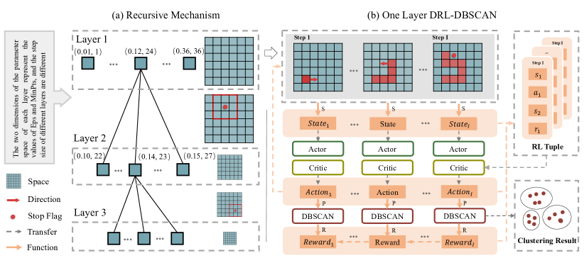
Figure 2. The core model of DRL-DBSCAN. (a) Recursive mechanism, takes $3$-layer $6\times 6$ parameter space as an example, with layerwise decreasing parameter space. (b) One layer DRL-DBSCAN, takes the search process in the $1$-th layer of the recursive mechanism as an example, aims to obtain the optimal parameter combination in the parameter space of layer $1$.

The proposed DRL-DBSCAN has a core model (Fig. 2) and four working modes (Fig. 3) that can be extended to downstream tasks. We firstly describe the basic Markov decision process for parameter search (Sec. 3.1), and the definition of the clustering parameter space and recursion mechanism (Sec. 3.2). Then, we explain the four DRL-DBSCAN working modes (Sec. 3.3).

3.1. Parameter Search with DRL

Faced with various clustering tasks, the fixed DBSCAN parameter search policy no longer has flexibility. We propose an automatic parameter search framework DRL-DBSCAN based on Deep Reinforcement Learning (DRL), in which the core model can be expressed as a Markov Decision Process $MDP(\mathcal{S},\mathcal{A},\mathcal{R},\mathcal{P})$ including state set, action space, reward function and policy optimization algorithm (Mundhenk et al., 2000). This process transforms the DBSCAN parameter search process into a maze game problem (Zheng et al., 2012; Bom et al., 2013) in the parameter space, aiming to train an agent to search for the end point parameters step by step from the start point parameters by interacting with the environment, and take the end point (parameters in the last step) as the final search result of an episode of the game (as shown in Fig. 2). Specifically, the agent regards the parameter space and DBSCAN clustering algorithm as the environment, the search position and clustering result as the state, and the parameter adjustment direction as the action. In addition, a small number of samples are used to reward the agent with exceptional behavior in a weakly supervised manner. We optimize the policy of agent based on the Actor-Critic (Konda and Tsitsiklis, 2000) architecture. Specifically, the search process for episode $e(e=1,2,...)$ is formulated as follows:

$\bullet$ State: Since the state needs to represent the search environment at each step as accurately and completely as possible, we consider building the representation of the state from two aspects.

Firstly, for the overall searching and clustering situation, we use a 7-tuple to describe the global state of the $i$-th step $(i=1,2,...)$:

(1) $$\bm{s}_{global}^{(e)(i)}=\bm{P}^{(e)(i)}\ {\cup}\ \mathcal{D}_{b}^{(e)(i)}\ {\cup}\ \big{\{}{R}_{cn}^{(e)(i)}\big{\}}.$$

Here, $\bm{P}^{(e)(i)}=\{Eps^{(e)(i)}$, $MinPts^{(e)(i)}\}$ is the current parameter combination. $\mathcal{D}_{b}^{(e)(i)}$ is the set of quaternary distances, including the distances of $Eps^{(e)(i)}$ from its space boundaries ${B}_{Eps,1}$ and ${B}_{Eps,2}$, the distances of $MinPts^{(e)(i)}$ from its boundaries ${B}_{MinPts,1}$ and ${B}_{MinPts,2}$, ${R}_{cn}^{(e)(i)}=\frac{|\mathcal{C}^{(e)(i)}|}{|\mathcal{V}|}$ is the ratio of the number of clusters $|\mathcal{C}^{(e)(i)}|$ to the total object number of data block $|\mathcal{V}|$. Here, the specific boundaries of parameters will be defined in Sec.  3.2.

Secondly, for the description of the situation of each cluster, we define the $\{d+2\}$-tuple of the $i$-th local state of cluster $\bm{c}_{n}\in\mathcal{\mathcal{C}}$ as:

(2) $$\bm{s}_{local,n}^{(e)(i)}=\mathcal{X}_{cent,n}^{(e)(i)}\ {\cup}\ \big{\{}{D}^{(e)(i)}_{cent,n},\ |\bm{c}_{n}^{(e)(i)}|\big{\}}.$$

Here, $\mathcal{X}_{cent,n}^{(e)(i)}$ is the central object feature of the $\bm{c}_{n}$, and $d$ is its feature dimension. ${D}^{(e)(i)}_{cent,n}$ is the Euclidean distance from the cluster center object to the center object of the entire data block. $|\bm{c}_{n}^{(e)(i)}|$ means the number of objects contained in cluster $\bm{c}_{n}$.

Considering the change of the number of clusters at different steps in the parameter search process, we use the Attention Mechanism (Vaswani et al., 2017) to encode the global state and multiple local states into a fixed-length state representation:

(3) $$\bm{s}^{(e)(i)}=\sigma\Big{(}\bm{F}_{G}(\bm{s}_{global}^{(e)(i)})\ {\mathbin{\|}}\ \sum_{\bm{c}_{n}\in\mathcal{C}}\bm{\alpha}_{att,n}\cdot\bm{F}_{L}(\bm{s}_{local,n}^{(e)(i)})\Big{)},$$

where $\bm{F}_{G}$ and $\bm{F}_{L}$ are the Fully-Connected Network (FCN) for the global state and the local state, respectively. $\sigma$ represents the ReLU activation function. And $||$ means the operation of splicing. $\alpha_{att,n}$ is the attention weight of cluster $\bm{c}_{n}$, which is formalized as follows:

(4) $$\bm{\alpha}_{att,n}=\frac{\sigma\Big{(}\bm{F}_{S}\big{(}\bm{F}_{G}(\bm{s}_{global}^{(e)(i)})\ {\mathbin{\|}}\ \bm{F}_{L}(\bm{s}_{local,n}^{(e)(i)})\big{)}\Big{)}}{\sum_{\bm{c}_{n}\in\mathcal{C}}\sigma\Big{(}\bm{F}_{S}\big{(}\bm{F}_{G}(\bm{s}_{global}^{(e)(i)})\ {\mathbin{\|}}\ \bm{F}_{L}(\bm{s}_{local,n}^{(e)(i)})\big{)}\Big{)}}.$$

We concatenate the global state with the local state of each cluster separately, input it into a fully connected network $\bm{F}_{S}$ for scoring, and use the normalized score of each cluster as its attention coefficient. This approach establishes the attention to the global search situation when local clusters are expressed. At the same time, it also makes different types of cluster information have different weights in the final state expression, which increases the influence of important clusters on the state.

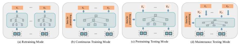
Figure 3. Four working modes. Dark orange square means partially labeled data, light orange square means unlabeled data.

$\bullet$ Action: The action $\bm{a}^{(e)(i)}$ for the $i$-th step is the search direction of parameter. We define the action space $\mathcal{A}$ as $\{left,right,$ $down,up,stop\}$, where $left$ and $right$ means to reduce or increase the $Eps$ parameter, $down$ and $up$ means to reduce or increase the $MinPts$ parameter, and $stop$ means to stop searching. Specifically, we build an Actor (Konda and Tsitsiklis, 2000) as the policy network to decide action $\bm{a}^{(e)(i)}$ based on the current state $\bm{s}^{(e)(i)}$:

(5) $$\bm{a}^{(e)(i)}=Actor(\bm{s}^{(e)(i)}).$$

Here, the $Actor$ is a three-layer Multi-Layer Perceptron (MLP).

In addition, the action-parameter conversion process from the $i$-th step to the $i+1$-th step is defined as follows.

(6) $$\bm{P}^{(e)(i)}\xrightarrow[]{\bm{a}^{(e)(i)},\ \bm{\theta}}\bm{P}^{(e)(i+1)}.$$

Here, $\bm{P}^{(e)(i)}$ and $\bm{P}^{(e)(i+1)}$ are the parameter combinations $\{Eps^{(e)(i)},$ $MinPts^{(e)(i)}\}$ and $\{Eps^{(e)(i+1)},MinPts^{(e)(i+1)}\}$ of the $i$-th step and the $i+1$-th step, respectively. $\bm{\theta}$ is the increase or decrease step size of the action. We discuss the step size in detail in Sec. 3.2. Note that when an action causes a parameter to go out of bounds, the parameter is set to the boundary value and the corresponding boundary distance is set to $-1$ in the next step.

$\bullet$ Reward: Considering that the exact end point parameters are unknown but rewards need to be used to motivate the agent to learn a better parameter search policy, we use a small number of samples of external metrics as the basis for rewards. We define the immediate reward function of the $i$-th step as:

(7) $$\mathcal{R}(\bm{s}^{(e)(i)},\bm{a}^{(e)(i)})={NMI}\big{(}DBSCAN(\mathcal{X},\bm{P}^{(e)(i+1)}),\mathcal{Y}^{\prime})\big{)}.$$

Here, ${NMI}(,)$ stands for the external metric function, Normalized Mutual Information (NMI) (Estévez et al., 2009) of $DBSCAN$ clustering. $\mathcal{X}$ is the feature set. $\mathcal{Y}^{\prime}$ is a set of partial labels of the data block. Note that the labels are only used in the training process, and the testing process performs search on unseen data blocks without labels.

In addition, the excellent parameter search action sequence for one episode is to adjust the parameters in the direction of the optimal parameters, and stop the search at the optimal parameters. Therefore, we consider using both the maximum immediate reward for subsequent steps and the endpoint immediate reward as the reward in the $i$-th step:

(8) $$\bm{r}^{(e)(i)}=\beta\cdot\max\big{\{}\mathcal{R}(\bm{s}^{(e)(m)},\bm{a}^{(e)(m)})\big{\}}|_{m=i}^{I}+\delta\cdot\mathcal{R}(\bm{s}^{(e)(I)},\bm{a}^{(e)(I)}),$$

where $\mathcal{R}(\bm{s}^{(e)(I)},\bm{a}^{(e)(I)})$ is the immediate rewards for the $I$-th step end point parameters. And max is used to calculate the future maximum immediate reward before stopping the search in current episode $e$. $\beta$ and $\delta$ are the impact factors of reward, where $\beta=1-\delta$.

$\bullet$ Termination: We determine the termination conditions for a complete episode search process as follows:

(9) $$\left\{\begin{array}[]{ll}\min(\mathcal{D}_{b}^{(e)(i)})<0,&\text{Out of bounds stop,}\\ i>=I_{max},&\text{Timeout stop,}\\ \bm{a}^{(e)(i)}=stop,where\ i\geq 2,&\text{Active stop.}\\ \end{array}\right.$$

Here, $I_{max}$ is the maximum search step size in an episode.

$\bullet$ Optimization: The parameter search process in the episode $e$ is expressed as: $1)$ observe the current state $\bm{s}^{(e)(i)}$ of DBSCAN clustering; $2)$ and predict the action $\bm{a}^{(e)(i)}$ of the parameter adjustment direction based on $\bm{s}^{(e)(i)}$ through the $Actor$; $3)$ then, obtain the new state $\bm{s}^{(e)(i+1)}$; $4)$ repeat the above process until the end of episode, and get reward $\bm{r}^{(e)(i)}$ for each step. The core element of the $i$-th step is extracted as:

(10) $$\mathcal{T}^{(e)(i)}=(\bm{s}^{(e)(i)},\bm{a}^{(e)(i)},\bm{s}^{(e)(i+1)},\bm{r}^{(e)(i)}).$$

We put $\mathcal{T}$ of each step into the memory buffer and sample $M$ core elements to optimize the policy network $Actor$, and define the key loss functions as follows:

$$\mathcal{L}_{c}={\sum}_{\mathcal{T}\in buffer}^{M}\big{(}\bm{r}^{(e)(i)}+\gamma\cdot Critic(\bm{s}^{(e)(i+1)},\bm{a}^{(e)(i+1)})-$$

(11) $$Critic(\bm{s}^{(e)(i)},\bm{a}^{(e)(i)})\big{)}^{2},$$

(12) $$\mathcal{L}_{a}=-\frac{{\sum}_{\mathcal{T}\in buffer}^{M}Critic\big{(}\bm{s}^{(e)(i)},Actor(\bm{s}^{(e)(i)})\big{)}}{M}.$$

Here, we define a three-layer MLP as the $Critic$ to learn the action value of state (Konda and Tsitsiklis, 2000), which is used to optimize the $Actor$. And $\gamma$ means reward decay factor. Note that we use the policy optimization algorithm named Twin Delayed Deep Deterministic strategy gradient algorithm (TD3) (Fujimoto et al., 2018) in our framework, and it can be replaced with other DRL policy optimization algorithms (Lillicrap et al., 2015; Konda and Tsitsiklis, 2000).

3.2. Parameter Space and Recursion Mechanism

In this section, we will define the parameter space of the agent proposed in the previous section and the recursive search mechanism based on different parameter spaces. Firstly, in order to deal with the fluctuation of the parameter range caused by different data distributions, we normalize the data features, thereby transforming the maximum $Eps$ parameter search range into the $(0,\sqrt{d}]$ range. Unlike $Eps$, the $MinPts$ parameter must be an integer greater than $0$. Therefore, we propose to delineate a coarse-grained $MinPts$ maximum parameter search range according to the size or dimension of the dataset. Subsequently, considering the large parameter space affects the efficiency when performing high-precision parameter search, we propose to use a recursive mechanism to perform a progressive search. The recursive process is shown in Fig. 2. We narrow the search range and increase the search precision layer by layer, and assign a parameter search agent $agent^{(l)}$ defined in Sec. 3.1 to each layer $l$ to search for the optimal parameter combination $\bm{P}_{o}^{(l)}=\{Eps_{o}^{(l)},MinPts_{o}^{(l)}\}$ under the requirements of the search precision and range of the corresponding layer. The minimum search boundary ${B}_{p,1}^{(l)}$ and maximum search boundary ${B}_{p,2}^{(l)}$ of parameter $p\in\{Eps,MinPts\}$ in the $l$-th layer $(l=1,2,...)$ are defined as:

(13) $$\begin{split}&{B}_{p,1}^{(l)}:\max\big{\{}{B}_{p,1}^{(0)},\ p_{o}^{(l-1)}-\frac{\pi_{p}}{2}\cdot\theta_{p}^{(l)}\big{\}},\\ &{B}_{p,2}^{(l)}:\min\big{\{}p_{o}^{(l-1)}+\frac{\pi_{p}}{2}\cdot\theta_{p}^{(l)},{B}_{p,2}^{(0)}\big{\}}.\\ \end{split}$$

Here, $\pi_{p}$ is the number of searchable parameters in the parameter space of parameter $p$ in each layer. ${B}_{p,1}^{(0)}$ and ${B}_{p,2}^{(0)}$ are the space boundaries of parameter $p$ in the $0$-th layer, which define the maximum parameter search range. $p_{o}^{(l-1)}\in\bm{P}_{o}^{(l-1)}$ is the optimal parameter searched by the previous layer, and $p_{o}^{(0)}\in\bm{P}_{o}^{(0)}$ is the midpoint of ${B}_{p,1}^{(0)}$ and ${B}_{p,2}^{(0)}$. In addition, $\theta_{p}^{(l)}$ is the search step size, that is, the search precision of the parameter $p$ in the $l$-th layer, which is defined as follows:

(14) $$\theta_{p}^{(l)}=\left\{\begin{array}[]{ll}\frac{\theta_{p}^{(l-1)}}{\pi_{p}},&{if\ p\ =\ Eps;}\\ \max\big{\{}\lfloor\frac{\theta_{p}^{(l-1)}}{\pi_{p}}+\frac{1}{2}\rfloor,\ 1\big{\}},&{otherwise.}\\ \end{array}\right.$$

Here, $\theta_{p}^{(l-1)}$ is the step size of the previous layer and $\theta_{p}^{(0)}$ is the size of the parameter maximum search range. $\lfloor\rfloor$ means round down.

Complexity Discussion: It is known that the minimum search step size of the recursive structure with layers $L$ is $\theta_{p}^{(L)}$. Then the computational complexity when there is no recursive structure is $O(N)$, where $N$ the size of the parameter space $\theta_{p}^{(0)}/\theta_{p}^{(L)}=(\pi_{p})^{L}$. And DRL-DBSCAN with $L$-layer recursive structure only takes $L\cdot(\pi_{p})$, reducing the complexity from $O(N)$ to $O(log\ N)$.

3.3. Proposed DRL-DBSCAN

Algorithm 1 shows the process of the proposed DRL-DBSCAN core model. Given a data block $\mathcal{V}$ with partial label $\mathcal{Y}^{\prime}$, the training process repeats the parameter search process (Lines 1-1) for multiple episodes at each layer to optimize the agent (Line 1). In this process, we update the optimal parameter combination (Line 1 and Line 1 based on the immediate reward (Eq. (7)). In order to improve efficiency, we build a hash table to record DBSCAN clustering results of searched parameter combinations. In addition, we established early stopping mechanisms to speed up the training process when the optimal parameter combination does not change (Line 1 and Line 1). It is worth noting that the testing process uses the trained agents to search directly with one episode, and does not set the early stop. Furthermore, the testing process does not need labels, and the end point parameters of the unique episode of the last layer are used as the final optimal parameter combination.

In order to better adapt to various task scenarios, we define four working modes of DRL-DBSCAN as shown in Fig. 3. Their corresponding definitions are as follows: (1) Retraining Mode ($DRL_{re}$). The optimal parameters are searched based on the training process. When the dataset changes, the agent at each layer is reinitialized. (2) Continuous Training Mode ($DRL_{con}$). The agents are pre-trained in advance. When the dataset changes, continue searching based on the training process using the already trained agents. (3) Pretraining Testing Mode ($DRL_{all}$). The agents are pre-trained in advance. When the dataset changes, searching directly based on the testing process without labels. (4) Maintenance Testing Mode ($DRL_{one}$). The agents are pre-trained in advance. When the dataset changes, searching directly based on the testing process without labels. After pre-training, regular maintenance training is performed with labeled historical data.

Input: The features $\mathcal{X}$ and partial labels $\mathcal{Y}^{\prime}$ of block $\mathcal{V}$; Agents for each layer: $\{agent^{(l)}\}|_{l=1}^{L_{max}}$;

Output: Optimal parameter combination: $\bm{P}_{o}$;

1 for $l=1,...,L_{max}$ do

2       Initialize parameter space via Eq. (13) and Eq. (14);

3       for $e=1,...,E_{max}$ do

4             Initialize $\bm{P}^{(e)(0)}$ by $\bm{P}_{o}^{(l-1)}$;

5             for $i=1,...,I_{max}$ do

6                   Obatin the current state $\bm{s}^{(e)(i)}$ via Eq. (3);

7                   Choose the action $\bm{a}^{(e)(i)}$ via Eq. (5);

8                   Get new parameters $\bm{P}^{(e)(i)}$ via Eq. (6);

9                   Clustering using the current parameters;

10                   Termination judgment via Eq. (9);

11                  

12            if is TRAIN then

13                   Get rewards $\bm{r}^{(e)(i)}$ via Eq. (8), $\forall i\in\{1,I\}$;

14                   Store $\mathcal{T}^{(e)(i)}$ in buffer via Eq. (10), $\forall i\in\{1,I\}$;

15                   Sampling and learning via Eq. (12) and Eq. (3.1);

16                  

17            Update optimal parameter combination $\bm{P}_{o}^{(l)}$;

18             Early stop judgment;

19            

20      Update optimal parameter combination $\bm{P}_{o}$;

21       Early stop judgment;

22      

Algorithm 1 The core model of DRL-DBSCAN

4. EXPERIMENTS

In this section, we conduct experiments mainly including the following: (1) performance comparison over DRL-DBSCAN and baseline in offline tasks, and explanation of the search process for Reinforcement Learning (RL) (Sec. 4.2); (2) performance analysis of DRL-DBSCAN and its variants, and advantage comparison between four working modes in online tasks (Sec. 4.3); (3) sensitivity analysis of hyperparameters and their impact on the model (Sec. 4.4).

4.1. Experiment Setup

Datasets. To fully analyze our framework, the experimental dataset consists of $4$ artificial clustering benchmark datasets and $1$ public real-world streaming dataset (Table 1). The benchmark datasets (Fränti and Sieranoja, 2018) are the $2D$ shape sets, including: Aggregation (Gionis et al., 2007), Compound (Zahn, 1971), Pathbased (Chang and Yeung, 2008), and D31 (Veenman et al., 2002). They involve multiple density types such as clusters within clusters, multi-density, multi-shape, closed loops, etc., and have various data scales. Furthermore, the real-world streaming dataset Sensor (Zhu, 2010) comes from consecutive information (temperature, humidity, light, and sensor voltage) collected from $54$ sensors deployed by the Intel Berkeley Research Lab. We use a subset of $80,864$ for experiments and divide these objects into $16$ data blocks ($\mathcal{V}_{1},...,\mathcal{V}_{16}$) as an online dataset.

Baseline and Variants. We compare proposed DRL-DBSCAN with three types of baselines: (1) traditional hyperparameter search schemes: random search algorithm Rand (Bergstra and Bengio, 2012), Bayesian optimization based on Tree-structured Parzen estimator algorithm BO-TPE (Bergstra et al., 2011); (2) meta-heuristic optimization algorithms: the simulated annealing optimization Anneal (Kirkpatrick et al., 1983), particle swarm optimization PSO (Shi and Eberhart, 1998), genetic algorithm GA (Lessmann et al., 2005), and differential evolution algorithm DE (Qin et al., 2008); (3) existing DBSCAN parameter search methods: KDist (V-DBSCAN) (Liu et al., 2007) and BDE-DBSCAN (Karami and Johansson, 2014). The detailed introduction to the above methods are given in Sec. 5. We also implement four variants of DRL-DBSCAN to analysis of state, reward and recursive mechanism settings in Sec. 3.1. Compared with DRL-DBSCAN, $DRL_{no-att}$ does not join local state based on the attention mechanism, $DRL_{only-max}$ only uses the maximum future immediate reward as final reward, $DRL_{recu}$ has no early stop mechanism, and $DRL_{recu}$ has no recursion mechanism.

Implementation Details. For all baselines, we use open-source implementations from the benchmark library Hyperopt (Bergstra et al., 2013) and Scikit-opt (_20, 2022), or provided by the author. All experiments are conducted on Python 3.7, $36$ core $3.00$GHz Intel Core $i9$ CPU, and NVIDIA RTX $A6000$ GPUs.

Experimental Setting. The evaluation of DRL-DBSCAN is based on the four working modes proposed in Sec.  3.3. Considering the randomness of most algorithms, all experimental results we report are the means or variances of $10$ runs with different seeds (except KDist because it’s heuristic and doesn’t involve random problems). Specifically, for the pre-training and maintenance training processes of DRL-DBSCAN, we set the maximum number of episodes $E_{max}$ to $50$, and do not set the early stop mechanism. For the training process for searching, we set the maximum number of episodes $E_{max}$ to $15$. In offline tasks and online tasks, the maximum number of recursive layers $L_{max}$ is $3$ and $6$, respectively, and the maximum search boundary in the $0$-th layer of $MinPts$ ${B}_{MinPts,2}^{(0)}$ is $0.25$ and $0.0025$ times the size of block, respectively. In addition, we use the unified label training proportion $0.2$, the $Eps$ parameter space size $\pi_{Eps}$ $5$, the $MinPts$ parameter space size $\pi_{MinPts}$ $4$, the maximum number of search steps $I_{max}$ $30$ and the reward factor $\delta$ $0.2$. The FCN and MLP dimensions are uniformly set to $32$ and $256$, the reward decay factor $\gamma$ of Critic is $0.1$, and the number of samples $M$ from the buffer is $16$. Furthermore, all baselines use the same objective function (Eq. (7)), parameter search space, and parameter minimum step size as DRL-DBSCAN if they support the settings.

Evaluation Metrics. We evaluate the experiments in terms of accuracy and efficiency. Specifically, we measure the clustering accuracy based on normalized mutual information (NMI) (Estévez et al., 2009) and adjusted rand index (ARI) (Vinh et al., 2010). For the efficiency, we use the consumed DBSCAN clustering rounds as the measurement.

4.2. Offline Evaluation

Offline evaluation is based on four artificial benchmark datasets. Since there is no data for pre-training in offline scenarios, we only compare the parameter search performance of DRL-DBSCAN using the retraining mode $DRL_{re}$ with baselines.

Accuracy and Stability Analysis. In Table 2, we summarize the means and variances of the NMI and ARI corresponding to the optimal DBSCAN parameter combinations that can be searched by $DRL_{re}$ and baselines within $30$ clustering rounds. It can be seen from the mean accuracy results of ten runs that in the Pathbased, Compound, Aggregation, and D31 datasets, $DRL_{re}$ can effectively improve the performance of $4\%$ & $6\%$, $3\%$ & $3\%$, $20\%$ & $26\%$ and $5\%$ & $26\%$ on NMI and ARI, relative to the best performing baselines. At the same time, as the dataset size increases, the advantage of $DRL_{re}$ compared to other baselines in accuracy gradually increases. Furthermore, the experimental variances shows that $DRL_{re}$ improves stability by $4\%$ & $6\%$, $1\%$ & $1\%$, $9\%$ & $13\%$ and $2\%$ & $17\%$ on NMI and ARI, relative to the best performing baselines. The obvious advantages in terms of accuracy and stability indicate that $DRL_{re}$ can stably find excellent parameter combinations in multiple rounds of parameter search, compared with other hyperparameter optimization baselines under the same objective function. Besides, $DRL_{re}$ is not affected by the size of the dataset. Among all the baselines, PSO and DE are relatively worse in terms of accuracy, because their search in the parameter space is biased towards continuous parameters, requiring more rounds to achieve optimal results. BO-TPE learns previously searched parameter combinations through a probabilistic surrogate model and strikes a balance between exploration and exploitation, with significant advantages over other baselines. The proposed DRL-DBSCAN not only narrows the search space of parameters of each layer progressively through a recursive structure, but also learns historical experience, which is more suitable for searching DBSCAN clustering parameter combinations.

Table 1. Characteristics of Datasets.

Type	Dataset	Classes	Size	Dim.	Time
Offline	Pathbased	$3$	$300$	$2$	$\times$
	Compound	$6$	$399$	$2$	$\times$
	Aggregation	$7$	$788$	$2$	$\times$
	D31	$31$	$3100$	$2$	$\times$
Online	Sensor	$54$	$80640$	$5$	$\checkmark$

Efficiency Analysis. We present the average historical maximum NMI results for $DRL_{re}$ and all baselines when consuming a different number of clustering rounds in Fig. 4. The shade in the figure represents the fluctuation range (variance) of NMI in multiple runs (only BO-TPE is also shown with shade as the representative in the baselines). The results suggest that in the four datasets, $DRL_{re}$ can maintain a higher speed of finding better parameters than baselines, and fully surpass all baselines after the $5$-th, $12$-th, $17$-th, and $16$-th rounds, respectively. In the Pathbased dataset, the clustering rounds of $DRL_{re}$ is $2.49$ times faster than that of BO-TPE when the NMI of the parameter combination searched by $DRL_{re}$ reaches $0.72$. Besides, the results show that, with the increase of clustering rounds, the shadow area of the $DRL_{re}$ curve gradually decreases, while the shadow range of BO-TPE tends to be constant. The above observation also demonstrates the good stability of the search when the number of rounds of DRL-DBSCAN reaches a specific number.

DRL-DBSCAN Variants. We compare the $DRL_{recu}$ with $DRL_{no-recu}$ which without the recursion mechanism in Fig. 5. Note that, for $DRL_{recu}$, we turn off the early stop mechanism so that it can search longer to better compare with $DRL_{no-recu}$. The results show that the first $100$ episodes of the recursive mechanism bring the maximum search speedup ratio of $6.5$, which effectively proves the contribution of the recursive mechanism in terms of efficiency.

Table 2. Offline evaluation performance. The best results are bolded and second-best are underlined.

Dataset	Metrics	Traditional		Meta-heuristic				Dedicated
		Rand	BO-TPE	Anneal	PSO	GA	DE	KDist	BDE	DRLre	(Mean)	(Var.)
	NMI	.66$\pm$.23	.78$\pm$.07	.65$\pm$.24	.60$\pm$.28	.68$\pm$.19	.22$\pm$.28	.40$\pm$.- -	.51$\pm$.33	.82$\pm$.03	$\uparrow$ .04	$\downarrow$ .04
Pathbased	ARI	.63$\pm$.21	.79$\pm$.10	.66$\pm$.25	.55$\pm$.38	.67$\pm$.26	.18$\pm$.28	.38$\pm$.- -	.48$\pm$.40	.85$\pm$.04	$\uparrow$ .06	$\downarrow$ .06
	NMI	.75$\pm$.05	.70$\pm$.24	.52$\pm$.36	.46$\pm$.34	.70$\pm$.25	.33$\pm$.35	.39$\pm$.- -	.72$\pm$.25	.78$\pm$.04	$\uparrow$ .03	$\downarrow$ .01
Compound	ARI	.73$\pm$.04	.68$\pm$.24	.51$\pm$.35	.42$\pm$.36	.68$\pm$.24	.31$\pm$.34	.39$\pm$.- -	.70$\pm$.25	.76$\pm$.03	$\uparrow$ .03	$\downarrow$ .01
	NMI	.76$\pm$.11	.72$\pm$.14	.75$\pm$.27	.59$\pm$.35	.75$\pm$.15	.28$\pm$.37	.60$\pm$.- -	.63$\pm$.28	.96$\pm$.02	$\uparrow$ .20	$\downarrow$ .09
Aggregation	ARI	.68$\pm$.16	.63$\pm$.19	.70$\pm$.27	.51$\pm$.37	.68$\pm$.19	.25$\pm$.35	.52$\pm$.- -	.54$\pm$.28	.96$\pm$.03	$\uparrow$ .26	$\downarrow$ .13
	NMI	.31$\pm$.33	.23$\pm$.24	.17$\pm$.19	.36$\pm$.33	.23$\pm$.20	.24$\pm$.26	.07$\pm$.- -	.41$\pm$.36	.67$\pm$.02	$\uparrow$ .26	$\downarrow$ .17
D31	ARI	.14$\pm$.26	.04$\pm$.05	.03$\pm$.04	.09$\pm$.22	.04$\pm$.04	.06$\pm$.09	.00$\pm$.- -	.21$\pm$.28	.26$\pm$.02	$\uparrow$ .05	$\downarrow$ .02

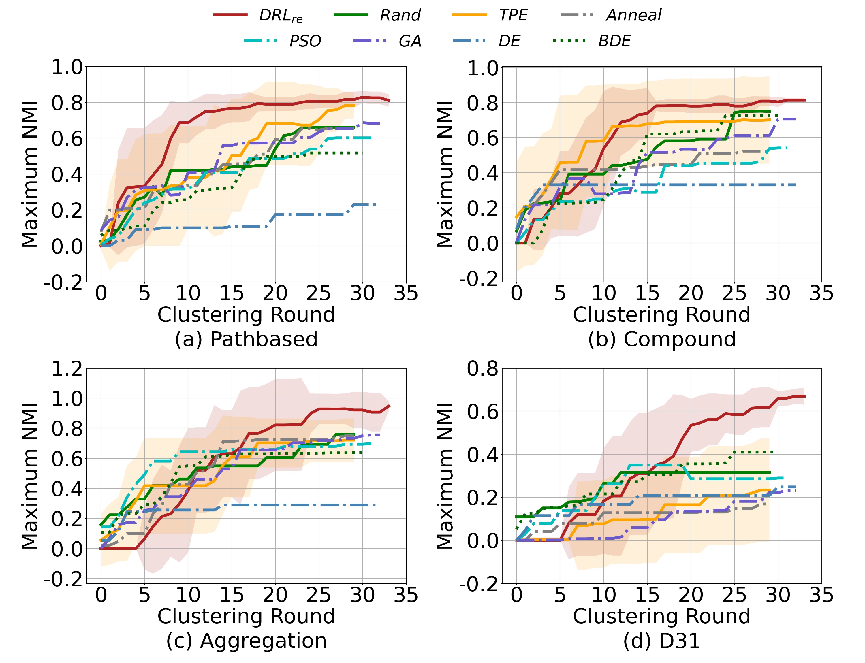
Figure 4. Offline clustering efficiency comparison.

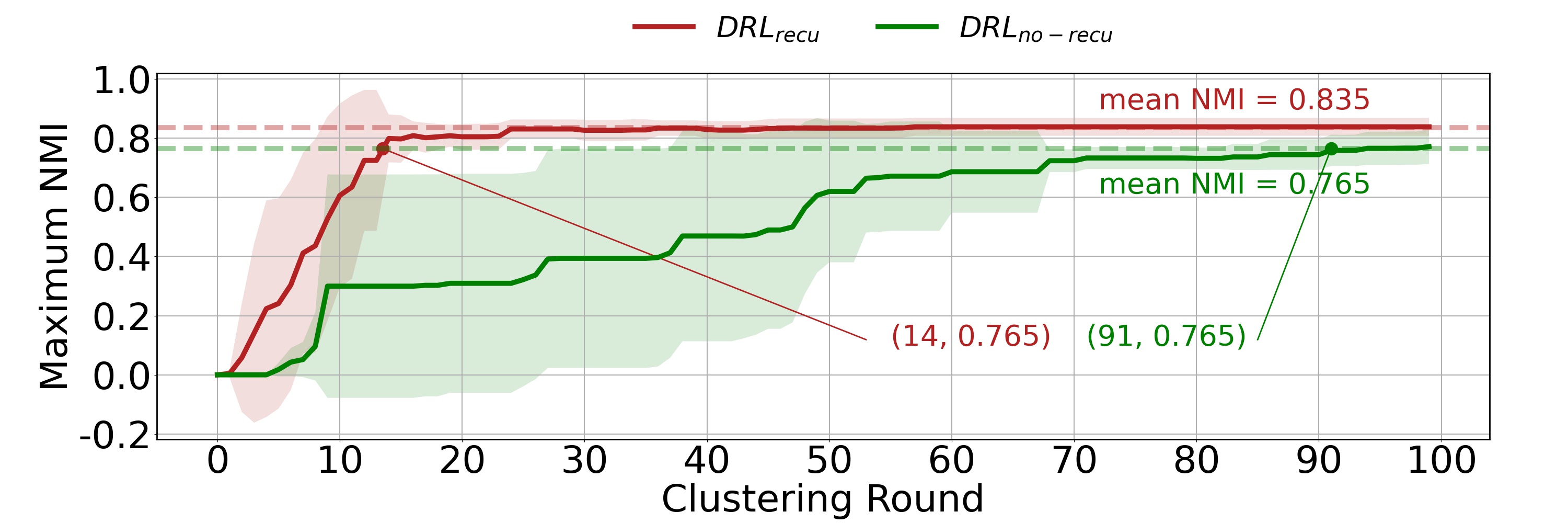
Figure 5. Efficiency comparison of recursive mechanism.

Label Proportion Comparison. Considering the influence of the proportion of labels participating in training on the DRL-DBSCAN training process’s reward and the objective function of other baselines, we conduct experiments with different label proportions in Pathbased, and the results are shown in Fig. 6(b) (the vertical lines above the histograms are the result variances). It can be seen that under different label proportions, the average NMI scores of $DRL_{re}$ are better than baselines, and the variance is also smaller. Additionally, as the proportion of labels decreases, the NMI scores of most of the baselines drop sharply, while the $DRL_{re}$ tends to be more or less constant. These stable performance results demonstrate the adaptability of DRL-DBSCAN to label proportion changes.

Case Study. To better illustrate the parameter search process based on RL, we take $3$ episodes in the $3$-rd recursive layer of the Pathbased dataset as an example for case study (Table 3). The columns in Table 3 are the action sequences made by the agent $agent^{(l)}$ in different episodes, the termination types of the episodes, the parameter combinations and NMI scores of the end point. We can observe that DRL-DBSCAN aims to obtain the optimal path from the initial parameter combination to the optimal parameter combination. The path-based form of search can use the optimal path learned in the past while retaining the ability to explore the unknown search direction for each parameter combination along the path. Since we add the $stop$ action to the action, DRL-DBSCAN can also learn how to stop at the optimal position, which helps extend DRL-DBSCAN to online clustering situations where there is no label at all. Note that we save the clustering information of the parameter combinations experienced in the past into a hash table, thereby no additional operations are required for repeated paths.

Table 3. Case study.

Action Sequence	Stop Type	$Eps$ / $MinPts$	NMI
$stop\rightarrow left\rightarrow up\rightarrow$	Out	$0.155$ / $41$	.64
$down\rightarrow down\rightarrow right\rightarrow$
$right\rightarrow right$
$down\rightarrow right\rightarrow up\rightarrow$	Active	$0.139$ / $41$	.74
$left\rightarrow down\rightarrow stop$
$left\rightarrow left$	Out	$0.123$ / $43$	.81

4.3. Online Evaluation

The learnability of RL enables DRL-DBSCAN to better utilize past experience in online tasks. To this end, we comprehensively evaluate four working modes of DRL-DBSCAN on a streaming dataset, Sensor. Specifically, the first eight blocks of the Sensor are used for the pre-training of $DRL_{con}$, $DRL_{all}$ and $DRL_{one}$, and the last eight blocks are used to compare the results with baselines. Since baselines cannot perform incremental learning for online tasks, we initialize the algorithm before each block starts like $DRL_{re}$. In addition, both experiments of $DRL_{all}$ and $DRL_{one}$ use unseen data for unlabeled testing, whereas $DRL_{one}$ uses the labeled historical data for model maintenance training after each block ends testing.

Table 4. Online evaluation NMI for training-based modes. The best results are bolded and second-best are underlined.

Blocks	Rand	BO-TPE	Anneal	PSO	GA	DE	KDist	BDE	DRLre	DRLcon	(Mean)	(Var.)
$\mathcal{V}_{9}$	.67$\pm$.24	.83$\pm$.03	.53$\pm$.37	.74$\pm$.10	.65$\pm$.29	.19$\pm$.31	.30$\pm$.- -	.70$\pm$.21	.86$\pm$.01	.87$\pm$.00	$\uparrow$ .04	$\downarrow$ .03
$\mathcal{V}_{10}$	.36$\pm$.15	.50$\pm$.07	.45$\pm$.17	.50$\pm$.20	.43$\pm$.15	.15$\pm$.17	.20$\pm$.- -	.37$\pm$.20	.50$\pm$.27	.64$\pm$.06	$\uparrow$ .14	$\downarrow$ .01
$\mathcal{V}_{11}$	.40$\pm$.06	.43$\pm$.10	.32$\pm$.26	.55$\pm$.16	.43$\pm$.08	.09$\pm$.12	.12$\pm$.- -	.47$\pm$.16	.60$\pm$.16	.68$\pm$.02	$\uparrow$ .13	$\downarrow$ .04
$\mathcal{V}_{12}$	.44$\pm$.23	.62$\pm$.16	.27$\pm$.35	.66$\pm$.07	.50$\pm$.24	.19$\pm$.28	.11$\pm$.- -	.41$\pm$.31	.75$\pm$.01	.72$\pm$.10	$\uparrow$ .09	$\downarrow$ .06
$\mathcal{V}_{13}$	.84$\pm$.06	.87$\pm$.04	.72$\pm$.38	.68$\pm$.26	.76$\pm$.17	.38$\pm$.38	.62$\pm$.- -	.68$\pm$.23	.92$\pm$.02	.92$\pm$.02	$\uparrow$ .08	$\downarrow$ .02
$\mathcal{V}_{14}$	.74$\pm$.12	.82$\pm$.04	.54$\pm$.37	.63$\pm$.24	.54$\pm$.24	.25$\pm$.25	.55$\pm$.- -	.56$\pm$.25	.76$\pm$.25	.85$\pm$.00	$\uparrow$ .03	$\downarrow$ .04
$\mathcal{V}_{15}$	.68$\pm$.24	.76$\pm$.04	.66$\pm$.34	.55$\pm$.25	.62$\pm$.27	.28$\pm$.32	.36$\pm$.- -	.72$\pm$.14	.85$\pm$.07	.83$\pm$.13	$\uparrow$ .17	-
$\mathcal{V}_{16}$	.73$\pm$.13	.77$\pm$.09	.77$\pm$.10	.40$\pm$.35	.67$\pm$.22	.49$\pm$.31	.11$\pm$.- -	.67$\pm$.19	.86$\pm$.01	.86$\pm$.00	$\uparrow$ .09	$\downarrow$ .09

Table 5. Online evaluation NMI for testing-based modes. The best results are bolded and second-best are underlined.

Blocks	Rand	BO-TPE	Anneal	PSO	GA	DE	KDist	BDE	DRLall	DRLone	(Mean)	(Var.)
$\mathcal{V}_{9}$	.34$\pm$.31	.49$\pm$.33	.22$\pm$.34	.14$\pm$.29	.27$\pm$.37	.10$\pm$.26	.30$\pm$.- -	.54$\pm$.36	.68$\pm$.30	.68$\pm$.30	$\uparrow$ .19	-
$\mathcal{V}_{10}$	.11$\pm$.14	.28$\pm$.17	.17$\pm$.21	.24$\pm$.01	.20$\pm$.21	.12$\pm$.18	.20$\pm$.- -	.28$\pm$.24	.33$\pm$.16	.33$\pm$.15	$\uparrow$ .05	-
$\mathcal{V}_{11}$	.16$\pm$.15	.29$\pm$.24	.23$\pm$.18	.33$\pm$.29	.23$\pm$.23	.02$\pm$.05	.12$\pm$.- -	.21$\pm$.22	.30$\pm$.13	.32$\pm$.08	-	-
$\mathcal{V}_{12}$	.23$\pm$.25	.19$\pm$.24	.10$\pm$.22	.38$\pm$.26	.34$\pm$.27	.03$\pm$.06	.11$\pm$.- -	.29$\pm$.27	.38$\pm$.17	.46$\pm$.09	$\uparrow$ .08	-
$\mathcal{V}_{13}$	.58$\pm$.35	.70$\pm$.24	.47$\pm$.40	.44$\pm$.31	.36$\pm$.28	.08$\pm$.14	.62$\pm$.- -	.32$\pm$.26	.68$\pm$.34	.70$\pm$.27	-	-
$\mathcal{V}_{14}$	.36$\pm$.19	.34$\pm$.28	.47$\pm$.35	.37$\pm$.33	.27$\pm$.25	.11$\pm$.24	.55$\pm$.- -	.43$\pm$.28	.60$\pm$.27	.62$\pm$.16	$\uparrow$ .15	$\downarrow$ .03
$\mathcal{V}_{15}$	.45$\pm$.35	.38$\pm$.36	.37$\pm$.33	.30$\pm$.34	.36$\pm$.32	.09$\pm$.18	.36$\pm$.- -	.42$\pm$.31	.64$\pm$.28	.70$\pm$.03	$\uparrow$ .25	$\downarrow$ .15
$\mathcal{V}_{16}$	.22$\pm$.32	.45$\pm$.24	.32$\pm$.29	.19$\pm$.27	.36$\pm$.27	.12$\pm$.20	.11$\pm$.- -	.59$\pm$.23	.60$\pm$.27	.53$\pm$.20	$\uparrow$ .01	-

Accuracy and Stability Analysis. We give the performance comparison of training-based modes ($DRL_{re}$ and $DRL_{con}$) and testing-based modes ($DRL_{all}$ and $DRL_{one}$) of DRL-DBSCAN with the baselines in Table 4 and Table 5, respectively. Due to the action space of DRL-DBSCAN has the $stop$ action, it can automatically terminate the search. To control the synchronization of baselines’ experimental conditions, we use the average clustering rounds consumed when DRL-DBSCAN is automatically terminated as the maximum round of baselines for the corresponding task ($30$ for Table 4 and $16$ for Table 5). The results show that the means of NMI scores of the training-based and testing-based search modes are improved by about $9\%$ and $9\%$ on average over multiple blocks, respectively, and the variances of performance are reduced by about $4\%$ and $2\%$, respectively. Specifically, Table 4 firstly shows that similar to the offline tasks, $DRL_{re}$, which is based on re-training, still retains the significant advantage in online tasks. Secondly, compared $DRL_{con}$ which is capable of continuous incremental learning with $DRL_{re}$, $DRL_{con}$ has a performance improvement of up to $14\%$ with a significant decrease in variance. Third, from Table 5, it can be found that in testing-based modes, $DRL_{all}$ and $DRL_{one}$ without labels (without reward function) can significantly exceed the baselines that require labels to establish the objective function. Fourth, $DRL_{one}$ which is regularly maintained has higher performance and less variance than $DRL_{all}$. These results demonstrate the capability of DRL-DBSCAN to retain historical experience and the advantages of learnable DBSCAN parameter search for accuracy and stability. In addition, although KDist can determine parameters without labels and iterations, its accuracy is relatively low.

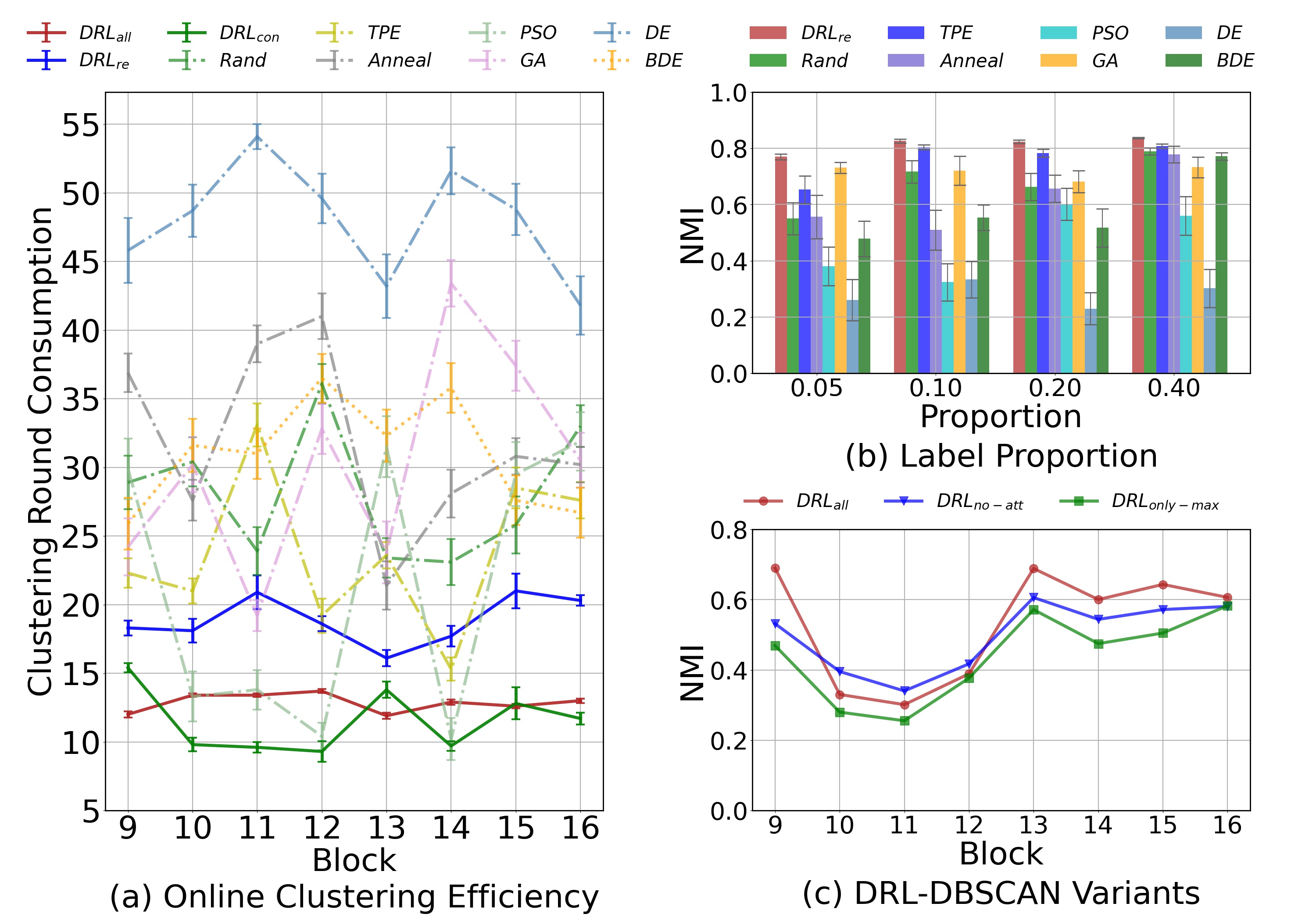
Figure 6. Comparison in online and offline tasks.

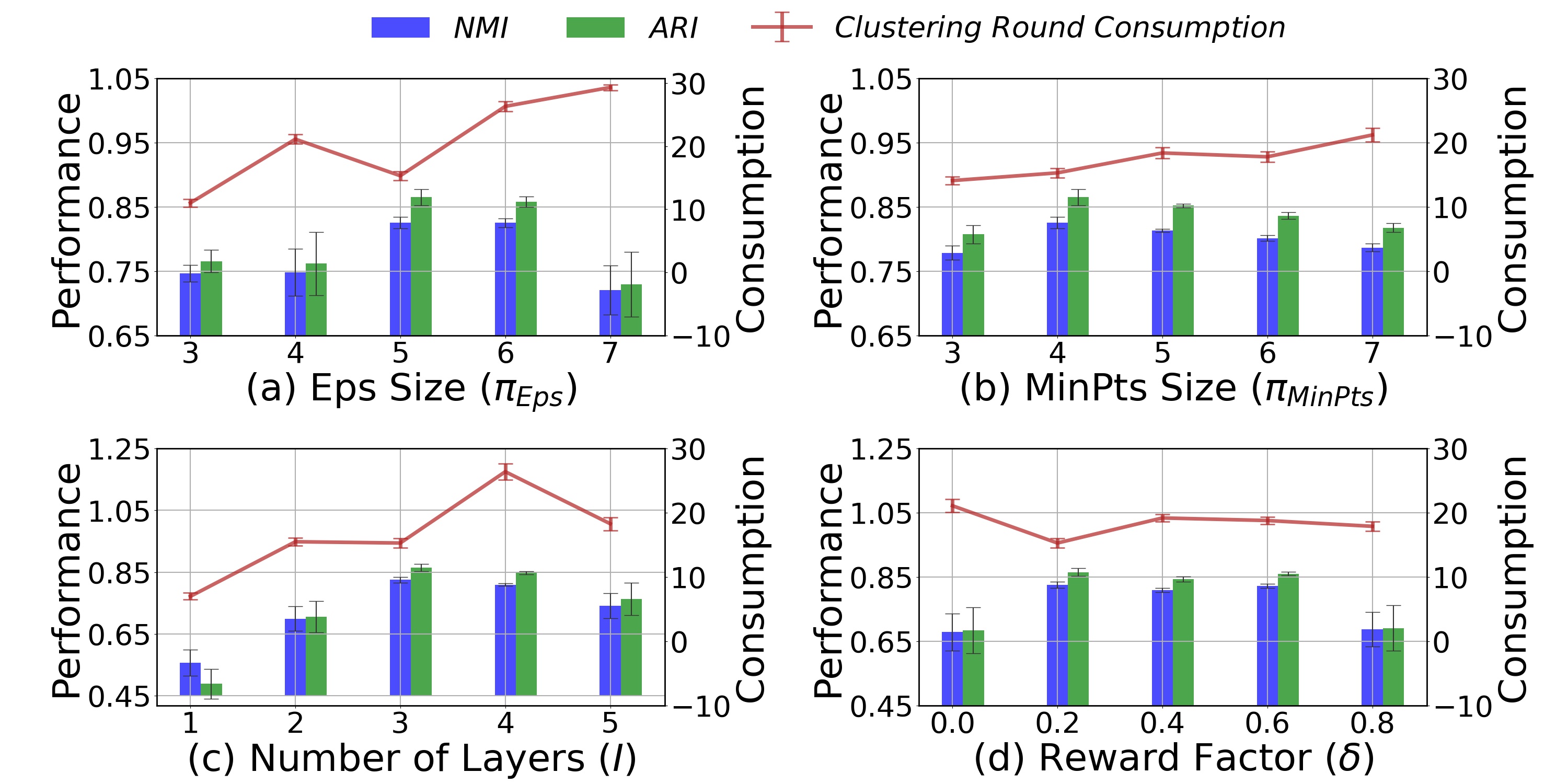
Figure 7. Parameter sensitivity.

Efficiency Analysis. $DRL_{all}$ and $DRL_{one}$ automatically search for the optimal DBSCAN parameters (end point parameters) without labels. In order to better analyze these two testing-based parameter search modes, we compare the number of clustering rounds required of other methods to reach the NMI scores of the $DRL_{all}$ end-point parameters in the online tasks (Fig. 6(a)). In the figure, the short vertical lines are the result variances. We can see that $DRL_{all}$ reaches the optimal results within the consumption range of $11$-$14$ rounds, while other baselines require more rounds when reaching the corresponding NMI. Moreover, many baselines’ round consumption over different blocks fluctuates significantly, and the variance in the same block is also large. The above observation suggests that the parameter search efficiency of DRL-DBSCAN’s testing-based modes without labels exceeds that of the baselines which require labels. Additionally, $DRL_{con}$ consumes fewer rounds than $DRL_{re}$ when reaching the same NMI, which also proves the advantage of DRL-DBSCAN’s learning ability in terms of efficiency.

DRL-DBSCAN Variants. To better evaluate the design of states and rewards in Sec. 3.1, we compare two variants with $DRL_{all}$ in the online tasks, namely $DRL_{no-att}$ (state has no attention mechanism) and $DRL_{only-max}$ (reward only based on future maximum immediate reward). The results in Fig. 6(c) show that the full structure of $DRL_{all}$ has better NMI scores than the variants, and brings the maximum performance increase of $0.16$, which represents the necessity of setting the local state and end point immediate reward.

4.4. Hyperparameter Sensitivity

Fig. 7 shows the results of the offline evaluation of $DRL_{re}$ on the Pathbased for four hyperparameters. Fig. 7(a) and Fig. 7(b) compare a set of parameter space sizes of $Eps$ and $MinPts$ involved in the Eq. (13), respectively. It can be found that the parameter space that is too large or too small for $Eps$ will cause performance loss and a decrease in search efficiency, while $MinPts$ is less sensitive to the parameter space’s size change. Fig. 7(c) analyzes the effect of different numbers of recursive layers on the search results. The results show that a suitable number of recurrent layers helps to obtain stable performance results. It is worth noting that the number of layers does not require much tuning, as we use the early-stop mechanism described in Sec. 3.3 to avoid overgrowing layers. Fig. 7(d) compares the different influence weights of end point immediate reward and future maximum immediate reward on the final reward (Eq.8). The results show that equalizing the contribution of the two immediate rewards to the final reward can help improve the performance of the DRL-DBSCAN.

5. RELATED WORK

Automatic DBSCAN parameter determination. DBSCAN is heavily dependent on two sensitive parameters ($Eps$ and $MinPts$) requiring prior knowledge for tuning. Numerous works propose different solutions for tuning the above. OPTICS (Ankerst et al., 1999) is an extension of DBSCAN, which establishes cluster sorting based on reachability to obtain the $Eps$. However, it needs to pre-determine the appropriate value of $MinPts$, and the acquisition of $Eps$ needs to interact with the user. V-DBSCAN (Liu et al., 2007) and KDDClus (Mitra and Nandy, 2011) plot the curve by using the sorted distance of any object to its $k$-th nearest object, and use the significant change on the curve as a series of candidate values for the $Eps$ parameter. Similar methods include DSets-DBSCAN (Hou et al., 2016), Outlier (Akbari and Unland, 2016) and RNN-DBSCAN (Bryant and Cios, 2017), all of which require a fixed $MinPts$ value or a predetermined the number of nearest neighbors $k$, and the obtained candidate $Eps$ parameters may not be unique. Beside the above work, there are some works (Darong and Peng, 2012; Diao et al., 2018) that consider combining DBSCAN with grid clustering to judge the density trend of raw samples according to the size and shape of each data region through pre-determined grid partition parameters. Although these methods reduce the difficulty of parameter selection to a certain extent, they still require the user to decide at least one parameter heuristically, making them inflexible in changing data.

Hyperparameter Optimization. For the parameters of DBSCAN, another feasible parameter decision method is based on the Hyperparameter Optimization (HO) algorithm. The classic HO methods are model-free methods, including grid search (Darong and Peng, 2012) that searches for all possible parameters, and random search (Bergstra and Bengio, 2012) etc. Another approach is Bayesian optimization methods such as BO-TPE (Bergstra et al., 2011), SMAC (Hutter et al., 2011), which optimize search efficiency using prior experience. In addition, meta-heuristic optimization methods, such as simulated annealing (Kirkpatrick et al., 1983), genetic (Lessmann et al., 2005), particle swarm (Shi and Eberhart, 1998) and differential evolution (Qin et al., 2008), can solve non-convex, non-continuous and non-smooth optimization problems by simulating physical, biological and other processes to search (Yang and Shami, 2020). Based on meta-heuristic optimization algorithms, some works propose HO methods for DBSCAN. BDE-DBSCAN (Karami and Johansson, 2014) targets an external purity index, selects $MinPts$ parameters based on a binary differential evolution algorithm, and selects $Eps$ parameters using a tournament selection algorithm. MOGA-DBSCAN (Falahiazar et al., 2021) proposes the outlier-index as a new internal index method for the objective function and selects parameters based on a multi-objective genetic algorithm. Although HO methods avoid handcrafted heuristic decision parameters, they require an accurate objective function (clustering external/internal metrics) and cannot cope with the problem of unlabeled data and the error of internal metrics. While DRL-DBSCAN can not only perform DBSCAN clustering state-aware parametric search based on the objective function, but also retain the learned search experience and conduct searches without the objective function.

Reinforcement Learning Clustering. Recently, some works that intersect Reinforcement Learning (RL) and clustering algorithms have been proposed. For example, MCTS Clustering (Brehmer et al., 2020) in particle physics task builds high-quality hierarchical clusters through Monte Carlo tree search to reconstruct primitive elementary particles from observed final-state particles. (Grua and Hoogendoorn, 2018) which targets the health and medical domain leverages two clustering algorithms, and RL to cluster users who exhibit similar behaviors. Both of these works are field-specific RL clustering methods. Compared with DRL-DBSCAN, the Markov process they constructed is only applicable to fixed tasks, and is not a general clustering method. Besides the above work, (Bagherjeiran et al., 2005) proposes an improved K-Means clustering algorithm that selects the weights of distance metrics in different dimensions through RL. Although this method effectively improves the performance of traditional K-Means, it needs to pre-determine the number of clusters $k$, which has limitations.

6. CONCLUSION

In this paper, we propose an adaptive DBSCAN parameter search framework based on Deep Reinforcement Learning. In the proposed DRL-DBSCAN framework, the agents that modulate the parameter search direction by sensing the clustering environment are used to interact with the DBSCAN algorithm. A recursive search mechanism is devised to avoid the search performance decline caused by a large parameter space. The experimental results of the four working modes demonstrate that the proposed framework not only has high accuracy, stability and efficiency in searching parameters based on the objective function, but also maintains an effective performance when searching parameters without external incentives.

- (1)
- _20 (2022) 2022. scikit-opt. https://github.com/guofei9987/scikit-opt
- Akbari and Unland (2016) Zohreh Akbari and Rainer Unland. 2016. Automated determination of the input parameter of DBSCAN based on outlier detection. In Ifip international conference on artificial intelligence applications and innovations. Springer, 280–291.
- Ankerst et al. (1999) Mihael Ankerst, Markus M Breunig, Hans-Peter Kriegel, and Jörg Sander. 1999. OPTICS: Ordering points to identify the clustering structure. ACM Sigmod record 28, 2 (1999), 49–60.
- Bagherjeiran et al. (2005) Abraham Bagherjeiran, Christoph F Eick, and Ricardo Vilalta. 2005. Adaptive clustering: Better representatives with reinforcement learning. Department of Computer Science, University of Houston, Houston (2005).
- Bergstra et al. (2011) James Bergstra, Rémi Bardenet, Yoshua Bengio, and Balázs Kégl. 2011. Algorithms for hyper-parameter optimization. Advances in neural information processing systems 24 (2011).
- Bergstra and Bengio (2012) James Bergstra and Yoshua Bengio. 2012. Random search for hyper-parameter optimization. Journal of machine learning research 13, 2 (2012).
- Bergstra et al. (2013) James Bergstra, Daniel Yamins, and David Cox. 2013. Making a science of model search: Hyperparameter optimization in hundreds of dimensions for vision architectures. In International conference on machine learning. PMLR, 115–123.
- Bom et al. (2013) Luuk Bom, Ruud Henken, and Marco Wiering. 2013. Reinforcement learning to train Ms. Pac-Man using higher-order action-relative inputs. In 2013 IEEE Symposium on Adaptive Dynamic Programming and Reinforcement Learning (ADPRL). IEEE, 156–163.
- Brehmer et al. (2020) Johann Brehmer, Sebastian Macaluso, Duccio Pappadopulo, and Kyle Cranmer. 2020. Hierarchical clustering in particle physics through reinforcement learning. arXiv preprint arXiv:2011.08191 (2020).
- Bryant and Cios (2017) Avory Bryant and Krzysztof Cios. 2017. RNN-DBSCAN: A density-based clustering algorithm using reverse nearest neighbor density estimates. IEEE Transactions on Knowledge and Data Engineering 30, 6 (2017), 1109–1121.
- Chang and Yeung (2008) Hong Chang and Dit-Yan Yeung. 2008. Robust path-based spectral clustering. Pattern Recognition 41, 1 (2008), 191–203.
- Darong and Peng (2012) Huang Darong and Wang Peng. 2012. Grid-based DBSCAN algorithm with referential parameters. Physics Procedia 24 (2012), 1166–1170.
- Diao et al. (2018) Kejing Diao, Yongquan Liang, and Jiancong Fan. 2018. An improved DBSCAN algorithm using local parameters. In International CCF Conference on Artificial Intelligence. Springer, 3–12.
- Dulac-Arnold et al. (2015) Gabriel Dulac-Arnold, Richard Evans, Hado van Hasselt, Peter Sunehag, Timothy Lillicrap, Jonathan Hunt, Timothy Mann, Theophane Weber, Thomas Degris, and Ben Coppin. 2015. Deep reinforcement learning in large discrete action spaces. arXiv preprint arXiv:1512.07679 (2015).
- Ester et al. (1996) Martin Ester, Hans-Peter Kriegel, Jörg Sander, Xiaowei Xu, et al. 1996. A density-based algorithm for discovering clusters in large spatial databases with noise.. In kdd, Vol. 96. 226–231.
- Estévez et al. (2009) Pablo A Estévez, Michel Tesmer, Claudio A Perez, and Jacek M Zurada. 2009. Normalized mutual information feature selection. IEEE Transactions on neural networks 20, 2 (2009), 189–201.
- Falahiazar et al. (2021) Zeinab Falahiazar, Alireza Bagheri, and Midia Reshadi. 2021. Determining the Parameters of DBSCAN Automatically Using the Multi-Objective Genetic Algorithm. J. Inf. Sci. Eng. 37, 1 (2021), 157–183.
- Fan et al. (2021) Tianhui Fan, Naijing Guo, and Yujie Ren. 2021. Consumer clusters detection with geo-tagged social network data using DBSCAN algorithm: a case study of the Pearl River Delta in China. GeoJournal 86, 1 (2021), 317–337.
- Fan and Xu (2019) Z Fan and Xiaolong Xu. 2019. Application and visualization of typical clustering algorithms in seismic data analysis. Procedia Computer Science 151 (2019), 171–178.
- Francis et al. (2011) Ziad Francis, Carmen Villagrasa, and Isabelle Clairand. 2011. Simulation of DNA damage clustering after proton irradiation using an adapted DBSCAN algorithm. Computer methods and programs in biomedicine 101, 3 (2011), 265–270.
- Fränti and Sieranoja (2018) Pasi Fränti and Sami Sieranoja. 2018. K-means properties on six clustering benchmark datasets. Applied intelligence 48, 12 (2018), 4743–4759.
- Fujimoto et al. (2018) Scott Fujimoto, Herke Hoof, and David Meger. 2018. Addressing function approximation error in actor-critic methods. In International conference on machine learning. PMLR, 1587–1596.
- Gionis et al. (2007) Aristides Gionis, Heikki Mannila, and Panayiotis Tsaparas. 2007. Clustering aggregation. Acm transactions on knowledge discovery from data (tkdd) 1, 1 (2007), 4–es.
- Grua and Hoogendoorn (2018) Eoin Martino Grua and Mark Hoogendoorn. 2018. Exploring clustering techniques for effective reinforcement learning based personalization for health and wellbeing. In 2018 IEEE Symposium Series on Computational Intelligence (SSCI). IEEE, 813–820.
- Guan et al. (2018) Chun Guan, Yuen Kevin Kam Fung, and Yong Yue. 2018. Towards a Personalized Item Recommendation Approach in Social Tagging Systems Using Intuitionistic Fuzzy DBSCAN. In 2018 10th International Conference on Intelligent Human-Machine Systems and Cybernetics (IHMSC), Vol. 1. IEEE, 361–364.
- Hou et al. (2016) Jian Hou, Huijun Gao, and Xuelong Li. 2016. DSets-DBSCAN: A parameter-free clustering algorithm. IEEE Transactions on Image Processing 25, 7 (2016), 3182–3193.
- Huang et al. (2019) Mengxing Huang, Qili Bao, Yu Zhang, and Wenlong Feng. 2019. A hybrid algorithm for forecasting financial time series data based on DBSCAN and SVR. Information 10, 3 (2019), 103.
- Hutter et al. (2011) Frank Hutter, Holger H Hoos, and Kevin Leyton-Brown. 2011. Sequential model-based optimization for general algorithm configuration. In International conference on learning and intelligent optimization. Springer, 507–523.
- Kanervisto et al. (2020) Anssi Kanervisto, Christian Scheller, and Ville Hautamäki. 2020. Action space shaping in deep reinforcement learning. In 2020 IEEE Conference on Games (CoG). IEEE, 479–486.
- Karami and Johansson (2014) Amin Karami and Ronnie Johansson. 2014. Choosing DBSCAN parameters automatically using differential evolution. International Journal of Computer Applications 91, 7 (2014), 1–11.
- Kazemi-Beydokhti et al. (2017) Mohammad Kazemi-Beydokhti, Rahim Ali Abbaspour, and Masoud Mojarab. 2017. Spatio-Temporal Modeling of Seismic Provinces of Iran Using DBSCAN Algorithm. Pure & Applied Geophysics 174, 5 (2017).
- Kirkpatrick et al. (1983) Scott Kirkpatrick, C Daniel Gelatt Jr, and Mario P Vecchi. 1983. Optimization by simulated annealing. science 220, 4598 (1983), 671–680.
- Konda and Tsitsiklis (2000) Vijay R Konda and John N Tsitsiklis. 2000. Actor-critic algorithms. In Proceedings of the NIPS. 1008–1014.
- Kużelewska and Wichowski (2015) Urszula Kużelewska and Krzysztof Wichowski. 2015. A modified clustering algorithm DBSCAN used in a collaborative filtering recommender system for music recommendation. In International conference on dependability and complex systems. Springer, 245–254.
- Lai et al. (2019) Wenhao Lai, Mengran Zhou, Feng Hu, Kai Bian, and Qi Song. 2019. A new DBSCAN parameters determination method based on improved MVO. Ieee Access 7 (2019), 104085–104095.
- Lessmann et al. (2005) Stefan Lessmann, Robert Stahlbock, and Sven F Crone. 2005. Optimizing hyperparameters of support vector machines by genetic algorithms.. In IC-AI. 74–82.
- Li and Li (2007) Xinyan Li and Deren Li. 2007. Discovery of rules in urban public facility distribution based on DBSCAN clustering algorithm. In MIPPR 2007: Remote Sensing and GIS Data Processing and Applications; and Innovative Multispectral Technology and Applications, Vol. 6790. International Society for Optics and Photonics, 67902E.
- Lillicrap et al. (2015) Timothy P Lillicrap, Jonathan J Hunt, Alexander Pritzel, Nicolas Heess, Tom Erez, Yuval Tassa, David Silver, and Daan Wierstra. 2015. Continuous control with deep reinforcement learning. arXiv preprint arXiv:1509.02971 (2015).
- Liu et al. (2007) Peng Liu, Dong Zhou, and Naijun Wu. 2007. VDBSCAN: varied density based spatial clustering of applications with noise. In 2007 International conference on service systems and service management. IEEE, 1–4.
- Mitra and Nandy (2011) S. Mitra and Jay Nandy. 2011. KDDClus : A Simple Method for Multi-Density Clustering. In Proceedings of International Workshop on Soft Computing Applications and Knowledge Discovery (SCAKD). 72–76.
- Mohammed et al. (2018) Nwayyin Najat Mohammed, Micheal Cawthorne, and Adnan Mohsin Abdulazeez. 2018. Detection of Genes Patterns with an Enhanced Partitioning-Based DBSCAN Algorithm. Journal of information and communication engineering 4, 1 (2018), 188–195.
- Mundhenk et al. (2000) Martin Mundhenk, Judy Goldsmith, Christopher Lusena, and Eric Allender. 2000. Complexity of finite-horizon Markov decision process problems. Journal of the ACM (JACM) 47, 4 (2000), 681–720.
- Pavlis et al. (2018) Michalis Pavlis, Les Dolega, and Alex Singleton. 2018. A modified DBSCAN clustering method to estimate retail center extent. Geographical Analysis 50, 2 (2018), 141–161.
- Peng et al. (2022) Hao Peng, Ruitong Zhang, Shaoning Li, Yuwei Cao, Shirui Pan, and Philip Yu. 2022. Reinforced, incremental and cross-lingual event detection from social messages. IEEE Transactions on Pattern Analysis and Machine Intelligence (2022).
- Qin et al. (2008) A Kai Qin, Vicky Ling Huang, and Ponnuthurai N Suganthan. 2008. Differential evolution algorithm with strategy adaptation for global numerical optimization. IEEE transactions on Evolutionary Computation 13, 2 (2008), 398–417.
- Shi and Eberhart (1998) Yuhui Shi and Russell C Eberhart. 1998. Parameter selection in particle swarm optimization. In International conference on evolutionary programming. Springer, 591–600.
- Smiti and Elouedi (2012) Abir Smiti and Zied Elouedi. 2012. Dbscan-gm: An improved clustering method based on gaussian means and dbscan techniques. In 2012 IEEE 16th international conference on intelligent engineering systems (INES). IEEE, 573–578.
- Vaswani et al. (2017) Ashish Vaswani, Noam Shazeer, Niki Parmar, Jakob Uszkoreit, Llion Jones, Aidan N Gomez, Łukasz Kaiser, and Illia Polosukhin. 2017. Attention is all you need. Advances in neural information processing systems 30 (2017).
- Veenman et al. (2002) Cor J. Veenman, Marcel J. T. Reinders, and Eric Backer. 2002. A maximum variance cluster algorithm. IEEE Transactions on pattern analysis and machine intelligence 24, 9 (2002), 1273–1280.
- Vijay and Nanda (2019) Rahul Kumar Vijay and Satyasai Jagannath Nanda. 2019. A Variable -DBSCAN Algorithm for Declustering Earthquake Catalogs. In Soft Computing for Problem Solving. Springer, 639–651.
- Vinh et al. (2010) Nguyen Xuan Vinh, Julien Epps, and James Bailey. 2010. Information theoretic measures for clusterings comparison: Variants, properties, normalization and correction for chance. JMLR 11 (2010), 2837–2854.
- Wei et al. (2019) Jiabin Wei et al. 2019. Commercial Activity Cluster Recognition with Modified DBSCAN Algorithm: A Case Study of Milan. In 2019 IEEE International Smart Cities Conference (ISC2). IEEE, 228–234.
- Yang and Shami (2020) Li Yang and Abdallah Shami. 2020. On hyperparameter optimization of machine learning algorithms: Theory and practice. Neurocomputing 415 (2020), 295–316.
- Yang et al. (2014) Yan Yang, Bin Lian, Lian Li, Chen Chen, and Pu Li. 2014. DBSCAN clustering algorithm applied to identify suspicious financial transactions. In 2014 International Conference on Cyber-Enabled Distributed Computing and Knowledge Discovery. IEEE, 60–65.
- Zahn (1971) Charles T Zahn. 1971. Graph-theoretical methods for detecting and describing gestalt clusters. IEEE Transactions on computers 100, 1 (1971), 68–86.
- Zheng et al. (2012) Kun Zheng, Husheng Li, Robert C Qiu, and Shuping Gong. 2012. Multi-objective reinforcement learning based routing in cognitive radio networks: Walking in a random maze. In 2012 international conference on computing, networking and communications (ICNC). IEEE, 359–363.
- Zhou and Gao (2014) Hong Bo Zhou and Jun Tao Gao. 2014. Automatic method for determining cluster number based on silhouette coefficient. In Advanced Materials Research, Vol. 951. Trans Tech Publ, 227–230.
- Zhu (2010) X. Zhu. 2010. Stream Data Mining Repository. http://www.cse.fau.edu/~xqzhu/stream.html