A Simple Capacity-Achieving Scheme for Channels with Polarization-Dependent Loss

Abstract

We demonstrate, for a widely used model of channels with polarization dependent loss (PDL), that channel capacity is achieved by a simple interference cancellation scheme in conjunction with a universal precoder. Crucially, the proposed scheme is not only information-theoretically optimal, but it is also exceptionally simple and concrete. It transforms the PDL channel into separate scalar additive white Gaussian noise channels, allowing off-the-shelf coding and modulation schemes designed for such channels to approach capacity. The signal-to-noise ratio (SNR) penalty incurred under 6 dB of PDL is reduced to the information-theoretic minimum of a mere 1 dB as opposed to the 4 dB SNR penalty incurred under naive over-provisioning.

I Overview

Polarization-dependent loss (PDL) is a capacity-reducing impairment in polarization-division-multiplexed (PDM) coherent optical transmission systems [1, 2, 3, 4, 5]. PDL mitigation schemes have been studied in a flurry of recent works [6, 7, 4, 8, 5, 9, 10, 11, 12, 13, 14, 15, 16, 17] as well as older works [18, 19, 20, 21, 22]. Renewed interest in PDL stems from its expected impact on next-generation optical networks which are dense in PDL-inducing components such as reconfigurable add-drop multiplexers (ROADMs) [4, 23]. In this paper, we provide a careful information-theoretic analysis of PDL-impaired PDM channels, modelling them as compound channels [24] and, in accordance with these models, provide a provably optimal, simple, low-complexity PDL mitigation scheme.

Throughout this paper, we assume a common memoryless model for a PDL-impaired PDM channel with no insertion loss (IL) uncertainty and with the channel parameters being perfectly known to the receiver but unknown to the transmitter. This model is considered in [4, 8, 10, 13, 17, 20, 25, 11]. Our goal is to find a scheme which maximizes the rate of reliable communication that can be guaranteed, given a known worst-case PDL value. We provide a simple scheme that achieves this goal and reduces the problem to separate communication across scalar additive white Gaussian noise (AWGN) channels, so that standard coding and modulation schemes for such channels can be directly applied without loss of optimality.

Our results can be summarized as follows. Given a class of channels with a worst-case PDL value of

$$10\log_{10}\left(\frac{1+\alpha}{1-\alpha}\right)\text{ dB}$$

where $\alpha\in[0,1)$ is fixed, a fundamental asymptotic SNR penalty relative to a classical AWGN channel is incurred. This penalty depends on the extent to which the two polarizations are jointly processed. In particular, the SNR penalty is, under

• no joint coding or decoding,

  $$10\log_{10}\left(\frac{1}{1-\alpha}\right)\text{ dB;}$$ (1)

• joint coding with parallel and independent decoding,

  $$10\log_{10}\left(\frac{1}{1-\alpha^{2}}\right)\text{ dB;}$$ (2)

• and joint coding with joint or successive decoding,

  $$10\log_{10}\left(\frac{1}{\sqrt{1-\alpha^{2}}}\right)\text{ dB.}$$ (3)

The improved but suboptimal SNR penalty (2) can be achieved by schemes along the lines of those described in [14, 11]. The optimal (smallest possible) SNR penalty (3) is achieved by our proposed scheme which constitutes a simple precoder in combination with a linear minimum mean square error (LMMSE) plus successive interference cancellation (SIC) receiver. The precoder is judiciously chosen so that the effective channel matrix after interference cancellation is an orthogonal design [26, 27] in the channel parameters, i.e., is unconditionally orthogonal. The resulting precoders in the cases of real- and complex-valued channel matrices are essentially permutations of those considered in [14, 11, 10], but it is precisely this correct choice of permutation, or equivalently, interference cancellation order, that is vital to achieving (3).

The remainder of this paper is organized as follows. In Section II, we comment on relationships between our proposed scheme and analysis and existing work. In Section III, we analyze the capacity of a PDL-impaired channel as a compound channel [24] and establish some requisite background. We then provide capacity-achieving schemes in Sections IV and V for the cases of real- and complex-valued channel models, respectively, both of which are common in the PDL literature. In Section VI, we provide a coarse-grained performance analysis of the proposed scheme, some comments on practical considerations, and suggestions for future work. We end with concluding remarks in Section VII.

II Existing Schemes

II-A LMMSE-SIC Schemes

It is well-known in information theory that LMMSE-SIC schemes are capacity-achieving in a variety of multiple-input multiple-output (MIMO) AWGN channel settings, provided that perfect interference cancellation is performed (refer to, e.g., [28, Chapter 8]). This is practically accomplished by separately coding the transmitted data streams and performing the interference cancellation after forward error correction (FEC). Such schemes, apart from avoiding infeasibly complex joint maximum likelihood (ML) detection of data streams, effectively synthesize separate scalar sub-channels on which codes designed for scalar channels can be employed without loss of optimality. Such coded LMMSE-SIC schemes have also been experimentally validated in space-division-multiplexed (SDM) optical transmission systems [29, 30, 31] and thus are known to be practical.

Achievable information rates under LMMSE-SIC schemes were recently investigated by Chou and Kahn in [6] in the general context of mode-dependent loss (MDL) in SDM systems including PDL-impaired PDM systems as a special case. In [6], it is noted that, as is the case with slow fading wireless channels, such schemes are suboptimal under separate coding of data streams since the achievable rate is limited by the capacity of the worst sub-channel whose identity is not known at the transmitter.

In this paper, we demonstrate how this limitation of LMMSE-SIC can be bypassed in the special case of memoryless PDL with no IL uncertainty. In particular, we demonstrate that there exists a universal precoder which symmetrizes the channel so that the sum of the worst-case capacities of the sub-channels induced by LMMSE-SIC is equal to the worst-case sum of these capacities, rendering such a scheme optimal.

II-B Precoding with ML Detection

In [17, 16, 18, 19, 20, 13], space–time coding schemes from wireless communication are adapted to produce polarization–time codes which are typically paired with ML receivers. Moreover, in [4, 8], the authors consider precoding schemes which operate only across polarizations and in-phase and quadrature components to reduce the complexity of ML processing. Our work demonstrates that under our modelling assumptions, such schemes are of no information-theoretic benefit compared to simpler precoders along the lines of [11, 14] when combined with a carefully designed linear interference cancellation architecture and codes designed for scalar AWGN channels. In particular, any apparent performance differences are essentially shaping and coding gains that could be relegated, without loss of optimality, to the outer AWGN channel codes.

If, however, we include uncertainty in the polarization-average loss or IL in the channel model, as in [3], such schemes could, in principle, have better outage performance than the proposed scheme. Stated more concretely, in the presence of random PDL and random IL, adding an IL margin to the PDL margin (3) so as to guarantee a certain outage probability does not result in the smallest theoretically possible penalty—or equivalently, highest achievable information rate—for that outage probability. Indeed, there could exist schemes which enable reliable communication across capacity-equivalent channel realizations having combinations of high IL with low PDL and low PDL with high IL. We leave the quantification of what gains are left on the table in such a setting as a question for future work.

II-C Information-Theoretic Designs

While PDL mitigation schemes have been either analyzed or designed from an information-theoretic perspective in previous works such as [4, 8, 5], mutual information is not necessarily a proxy for practically achievable rates when the underlying channel is compound. For example, consider a pair of parallel AWGN channels with unknown SNR values $\mathsf{SNR}_{1}$ and $\mathsf{SNR}_{2}$ yet known constant sum-capacity $c$ so that

$$\frac{1}{2}\log_{2}\left(1+\mathsf{SNR}_{1}\right)+\frac{1}{2}\log_{2}\left(1+\mathsf{SNR}_{2}\right)=c\text{.}$$ (4)

Such a channel is referred to as a compound channel [24] with capacity $c$ since reliable communication at rate $c$ requires reliable communication across every parallel channel with arbitrary $\mathsf{SNR}_{1}$ and $\mathsf{SNR}_{2}$ satisfying (4). One cannot expect an off-the-shelf coded modulation scheme designed for a scalar AWGN channel with an SNR of $\mathsf{SNR}_{3}$ such that

$$c=\frac{1}{2}\log_{2}\left(1+\mathsf{SNR}_{3}\right)$$ (5)

to achieve the same performance on every parallel channel satisfying (4) as it does on the capacity-equivalent scalar channel. In fact, the problem of communication across a class of capacity-equivalent channels such as that described by (4) with a practical code is an instance of the long-studied, non-trivial problem of the design of universal codes (see, e.g., [32, 33, 34]). Therefore, invariance of mutual information across channel realizations under a certain PDL mitigation scheme does not guarantee achievability by concatenation with a practical code designed for scalar AWGN channels or simple modifications thereof.

Matters are further complicated when the parallel channels are correlated as in the case of PDL-impaired PDM channels. In such a situation, realization of an information-theoretic promise could require high-complexity joint ML processing across the polarizations, and even then, we still have no performance guarantees under concatenation with codes designed for scalar channels.

In contrast, the proposed scheme reduces the problem of communication across a PDL-impaired PDM channel entirely to the classical, well-understood problem of scalar AWGN communication. The scheme can thus be combined with standard practical coded modulation schemes designed for scalar AWGN channels such as those in [35, 36] without loss of optimality. The overall performance of the proposed scheme from a gap-to-capacity and frame error rate (FER) perspective is then fully characterized in terms of the same measures on scalar AWGN channels for the constituent coded modulation schemes.

III Capacity of a PDL-Impaired Channel

Throughout this paper, we will use boldface font for vectors and matrices with $(\cdot)_{ij}$ denoting the $ij$th entry of a matrix and non-boldface font with subscripts denoting the entries of a vector.

III-A Notions of Capacity and Compound Capacity

We begin by considering the situation of a real-valued channel matrix. Without loss of generality, we can assume that the input to the channel is real-valued with a complex input being interpreted as two uses of the real channel. In particular, we consider the two-parameter channel defined by

$$\underbrace{\begin{bmatrix}Y_{1}\\ Y_{2}\end{bmatrix}}_{\mathbf{Y}}=\underbrace{\begin{bmatrix}\sqrt{1+\gamma}&0\\ 0&\sqrt{1-\gamma}\end{bmatrix}}_{\mathbf{D}_{\gamma}}\underbrace{\begin{bmatrix}\cos\theta&-\sin\theta\\ \sin\theta&\cos\theta\end{bmatrix}}_{\mathbf{R}_{\theta}}\underbrace{\begin{bmatrix}X_{1}\\ X_{2}\end{bmatrix}}_{\mathbf{X}}+\underbrace{\begin{bmatrix}Z_{1}\\ Z_{2}\end{bmatrix}}_{\mathbf{Z}}$$

where $\gamma\in[-\alpha,\alpha]$ and $\theta\in[0,2\pi)$ representing a class of channels with up to

$$10\log_{10}\left(\frac{1+\alpha}{1-\alpha}\right)\text{ dB}$$ (6)

of PDL where $\alpha\in[0,1)$ is fixed. Moreover, $\mathbf{X}$ and $\mathbf{Z}$ are independent with $\mathbf{Z}$ being white Gaussian, denoted $\mathbf{Z}\sim\mathcal{N}(\mathbf{0},\mathbf{I}_{2})$, and $\mathbf{X}$ satisfying the power constraint

$$\mathbb{E}\left[\norm{\mathbf{X}}_{2}^{2}\right]\leq 2\cdot\mathsf{SNR}\text{.}$$ (7)

Note that while this model is inherently non-unitary (or non-orthogonal), it is energy-preserving when $\mathbb{E}\left[X_{1}^{2}\right]=\mathbb{E}\left[X_{2}^{2}\right]$. In particular, if $\mathbb{E}\left[X_{1}^{2}\right]=\mathbb{E}\left[X_{2}^{2}\right]$ and (7) holds with equality, then $\mathsf{SNR}$ is the ratio of the total received signal power to the total received noise power, i.e.,

$$\mathsf{SNR}=\frac{\mathbb{E}\left[\norm{\mathbf{D}_{\gamma}\mathbf{R}_{\theta}\mathbf{X}}_{2}^{2}\right]}{\mathbb{E}\left[\norm{\mathbf{Z}}_{2}^{2}\right]}$$ (8)

as expected.

A variety of notions of channel capacity can be considered. One notion is the classical Shannon capacity

$$C_{\mathsf{classical}}(\gamma,\theta,\mathsf{SNR})=\max_{f_{\mathbf{X}},\,\mathbb{E}\left[\norm{\mathbf{X}}_{2}^{2}\right]\leq 2\cdot\mathsf{SNR}}I(\mathbf{X};\mathbf{D}_{\gamma}\mathbf{R}_{\theta}\mathbf{X}+\mathbf{Z})$$

where $f_{\mathbf{X}}$ denotes the probability density of $\mathbf{X}$ and $I(\cdot;\cdot)$ denotes mutual information. This represents the rate that can be achieved when $\gamma$ and $\theta$ are known at the transmitter. This is a well-understood problem [37] but does not represent our situation in which $\gamma$ and $\theta$ are not known at the transmitter since round-trip delays are typically longer than the channel coherence time [25].

Another possibility is to assume some probability distribution over $\gamma$ and $\theta$ and define the ergodic capacity

$$C_{\mathsf{ergodic}}(\mathsf{SNR})=\mathbb{E}_{\gamma,\theta}\left[C_{\mathsf{classical}}(\gamma,\theta,\mathsf{SNR})\right]\text{.}$$

This represents the rate achievable when the transmitted codeword (or frame) spans many channel realizations, i.e., values of $\gamma$ and $\theta$. However, these parameters are typically slowly varying relative to the baud rate so that achieving the ergodic capacity would require averaging over a prohibitively large number of channel uses [4].

The appropriate notion of capacity in this scenario is that of compound capacity [24]. In particular, we define

$$C_{\mathsf{compound}}(\alpha,\mathsf{SNR})=\\ \max_{f_{\mathbf{X}},\,\mathbb{E}\left[\norm{\mathbf{X}}_{2}^{2}\right]\leq 2\cdot\mathsf{SNR}}\;\min_{\gamma\in[-\alpha,\alpha],\,\theta\in[0,2\pi)}\,I(\mathbf{X};\mathbf{D}_{\gamma}\mathbf{R}_{\theta}\mathbf{X}+\mathbf{Z})\text{.}$$ (9)

The compound capacity $C_{\mathsf{compound}}(\alpha,\mathsf{SNR})$ represents the rate of reliable communication that we can guarantee assuming that $\gamma$ and $\theta$ are chosen by nature (or an adversary) from the sets $[-\alpha,\alpha]$ and $[0,2\pi)$, respectively, and then fixed for the duration of the transmission, but are unknown to the transmitter which only knows $\alpha$ with the receiver knowing $\gamma$ and $\theta$.

Henceforth, we define the concise notation

$$C_{\alpha}(\mathsf{SNR})=C_{\mathsf{compound}}(\alpha,\mathsf{SNR})$$

and define the real scalar AWGN channel capacity function

$$C(\mathsf{SNR})=\frac{1}{2}\log_{2}(1+\mathsf{SNR})$$

and proceed to compute (9). A standard information-theoretic argument as in [37] will show that we can omit $\mathbf{R}_{\theta}$ from the calculation and take $X_{1}$ and $X_{2}$ to be independent with

$$X_{1} \sim\mathcal{N}(0,2\beta\mathsf{SNR})\text{,}$$

$$X_{2} \sim\mathcal{N}(0,2(1-\beta)\mathsf{SNR})\text{,}$$

and $\beta\in[0,1]$ a power allocation factor. The capacity calculation then reduces to

$$C_{\alpha}(\mathsf{SNR})=\\ \max_{\beta\in[0,1]}\,\min_{\gamma\in[-\alpha,\alpha]}\,C(2(1+\gamma)\beta\mathsf{SNR})+C(2(1-\gamma)(1-\beta)\mathsf{SNR})\text{.}$$

We begin with the inner minimization. Define $\gamma^{*}(\beta)$ by

$$\gamma^{*}(\beta)=\\ \operatorname*{argmin}_{\gamma\in[-\alpha,\alpha]}C(2(1+\gamma)\beta\mathsf{SNR})+C(2(1-\gamma)(1-\beta)\mathsf{SNR})\text{.}$$

For a fixed $\beta$, a simple convexity argument will show that

$$\gamma^{*}(\beta)=\begin{cases}\alpha&\text{if }\beta\leq 1/2\\ -\alpha&\text{if }\beta>1/2\\ \end{cases}\text{,}$$

i.e., that the worst-case PDL is always extremal. Proceeding to the outer maximization, define $\beta^{*}$ by

$$\beta^{*}=\\ \operatorname*{argmax}_{\beta\in[0,1]}C(2(1+\gamma^{*}(\beta))\beta\mathsf{SNR})+C(2(1-\gamma^{*}(\beta))(1-\beta)\mathsf{SNR})\text{.}$$

Elementary algebra shows that $\beta^{*}=1/2$, i.e., that the optimal power allocation is symmetric, and we get that

$$C_{\alpha}(\mathsf{SNR})=C((1+\alpha)\mathsf{SNR})+C((1-\alpha)\mathsf{SNR})\text{.}$$ (10)

Thus, we see that the compound capacity of a PDL-impaired channel (10) corresponds to the sum-capacity of the two polarizations when $\theta=0$, $\gamma=\pm\alpha$, and $\mathbb{E}\left[X_{1}^{2}\right]=\mathbb{E}\left[X_{2}^{2}\right]=\mathsf{SNR}$. While this result and analysis is implicit in previous works such as [4, 5], the framework of compound capacity formalizes the problem and allows us to reason more carefully about it.

Finally, we remark that compound capacity is essentially a proxy for outage capacity [3] when the channel parameters are random. In particular, the probability of outage is determined by the PDL distribution; a fixed outage probability translates to a bound on the PDL, i.e., a value for $\alpha$. A typical value is $\alpha=0.599$ corresponding to $6$ dB of PDL and an outage probability of $10^{-5}$ [4]. However, as noted earlier, a capacity-achieving scheme under the compound channel model considered in this paper is not outage optimal if we wish to additionally model uncertainty in the polarization-average loss or IL as in [3].

III-B Capacity Under Non-Joint Coding

Figure 1: Compound channel capacities, asymptotic approximations, and AWGN capacity all normalized by the number of real dimensions.

To simplify the exposition, we will work with high-SNR approximations and consider the use of zero-forcing (ZF) instead of LMMSE receivers first. However, we emphasize that every approximation is a rigorous asymptotic and is accompanied by a corresponding exact result. We define a high-SNR approximation to the capacity (9), denoted $\widetilde{C}_{\alpha}(\mathsf{SNR})$, by

$$\widetilde{C}_{\alpha}(\mathsf{SNR})=C((1-\alpha^{2})\mathsf{SNR})+C(\mathsf{SNR})\text{.}$$ (11)

It can be shown that

$$C_{\alpha}(\mathsf{SNR})=\widetilde{C}_{\alpha}(\mathsf{SNR})+\mathcal{O}(\mathsf{SNR}^{-1})$$

where the hidden constant depends on $\alpha$.

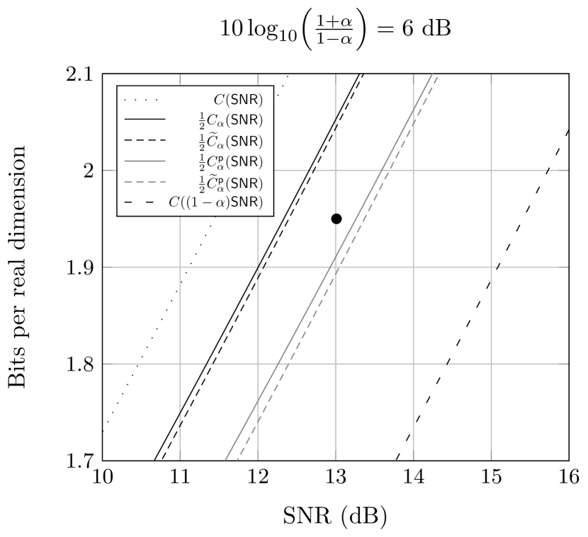
Figure 2: Close-up of Fig. 1. The solid circle is an operating point achievable by use of the proposed scheme in conjunction with the practical coded modulation scheme from [35] described in Section VI-B.

We will now establish the achievable rate under non-joint coding in which separate codewords are transmitted on each polarization and decoded separately. Henceforth, we will take $\mathbf{X}\sim\mathcal{N}(\mathbf{0},\mathsf{SNR}\mathbf{I}_{2})$ so that

$$I(X_{1}X_{2};Y_{1}Y_{2})=C((1+\gamma)\mathsf{SNR})+C((1-\gamma)\mathsf{SNR})$$ (12)

and

$$\min_{\gamma,\theta}I(X_{1}X_{2};Y_{1}Y_{2})=C_{\alpha}(\mathsf{SNR})$$

where the minimization is over $\gamma\in[-\alpha,\alpha]$ and $\theta\in[0,2\pi)$ with these sets suppressed for brevity. Note that by the chain rule of mutual information and independence of $X_{1}$ and $X_{2}$, we have (see, e.g., [38, Chapter 8]) that

$$I(X_{1}X_{2};Y_{1}Y_{2})=I(X_{1};Y_{1}Y_{2})+I(X_{2};Y_{1}Y_{2}X_{1})\text{.}$$ (13)

Moreover, one can compute (see, e.g., [38, Chapter 9]) that

$$I(X_{1};Y_{1}Y_{2})=\\ C((1+\gamma)\mathsf{SNR})+C((1-\gamma)\mathsf{SNR})-C((1-\gamma\cos(2\theta))\mathsf{SNR})$$

and that

$$I(X_{2};Y_{1}Y_{2}X_{1})=C((1-\gamma\cos(2\theta))\mathsf{SNR})$$

which add up to (12) as one expects from the chain rule of mutual information (13). Note that these mutual information terms in the chain rule of mutual information are precisely the capacities of the sub-channels induced by LMMSE-SIC when we have an AWGN MIMO channel (see, e.g., [28, Chapter 8] and [6]).

We then see that

$$C_{\alpha}(\mathsf{SNR}) =\min_{\gamma,\theta}I(X_{1}X_{2};Y_{1}Y_{2})$$

$$=\min_{\gamma,\theta}\big{[}I(X_{1};Y_{1}Y_{2})+I(X_{2};Y_{1}Y_{2}X_{1})\big{]}$$

$$\geq\min_{\gamma,\theta}I(X_{1};Y_{1}Y_{2})+\min_{\gamma,\theta}I(X_{2};Y_{1}Y_{2}X_{1})$$

$$=2C((1-\alpha)\mathsf{SNR})$$

which highlights the fundamental problem of communication across this channel. This problem is the mismatch between the minimum of the sum and the sum of the minima of the capacities of the two polarizations. Therefore, if each polarization is treated as a separate channel, we can only guarantee a rate of $C((1-\alpha)\mathsf{SNR})$ on each even if we perfectly remove the interference from one of them.

Note, however, that this achievable rate is a highly pessimistic baseline since merely interleaving a bit stream across the two polarizations constitutes a form of joint coding and could result in a smaller penalty than (1).

III-C Parallel Capacity

We now define the capacity achievable under a parallel decoding architecture whereby no interference cancellation or decision feedback across the polarizations is allowed. Noting that

$$I(X_{1}X_{2};Y_{1}Y_{2})\geq I(X_{1};Y_{1}Y_{2})+I(X_{2};Y_{1}Y_{2})\text{,}$$

and that

$$I(X_{2};Y_{1}Y_{2})=\\ C((1+\gamma)\mathsf{SNR})+C((1-\gamma)\mathsf{SNR})-C((1+\gamma\cos(2\theta))\mathsf{SNR})\text{,}$$

we define and compute the parallel capacity $C_{\alpha}^{\mathsf{p}}(\mathsf{SNR})$ as

$$C_{\alpha}^{\mathsf{p}}(\mathsf{SNR}) =\min_{\gamma,\theta}\big{[}I(X_{1};Y_{1}Y_{2})+I(X_{2};Y_{1}Y_{2})\big{]}$$

$$=2C_{\alpha}(\mathsf{SNR})-2C(\mathsf{SNR})$$

$$=2\widetilde{C}_{\alpha}(\mathsf{SNR})-2C(\mathsf{SNR})+\mathcal{O}(\mathsf{SNR}^{-1})$$

$$=2C((1-\alpha^{2})\mathsf{SNR})+\mathcal{O}(\mathsf{SNR}^{-1})\text{,}$$

where we have substituted the approximation (11). We accordingly define a high-SNR approximation for the parallel capacity $\widetilde{C}_{\alpha}^{\mathsf{p}}(\mathsf{SNR})$ by

$$\widetilde{C}_{\alpha}^{\mathsf{p}}(\mathsf{SNR})=2C((1-\alpha^{2})\mathsf{SNR})\text{.}$$

These results are plotted in Fig. 1 and Fig. 2 for $\alpha=0.599$ which corresponds to a $6$ dB worst-case PDL. One can see from the figures penalties relative to a PDL-free channel of roughly $1$ dB under an optimal scheme, $2$ dB under a parallel scheme, and $4$ dB under a non-joint scheme. Alternatively, these penalties at high SNR can be computed by (1), (2), and (3). Moreover, we remark that in the limit of high PDL, i.e., $\alpha$ approaching $1$, the SNR penalties become infinite: not because the capacity approaches zero, but because its growth rate is halved relative to the reference PDL-free channel.

III-D AWGN Channels Induced by Linear Equalization

Before proceeding to describe our capacity-achieving schemes, we will review—for the reader’s convenience—the method of calculating SNRs and noise statistics under linear precoding and equalization with possible interference cancellation. Moreover, note that for the remainder of this paper, we may redefine previously used notation where appropriate.

The effective channel after precoding and possibly interference cancellation is given by

$$\mathbf{Y}=\mathbf{H}\mathbf{U}+\mathbf{Z}$$

where $\mathbf{H}\in\mathbb{R}^{m\times n}$ with $m\geq n$,

$$\mathbb{E}\left[\mathbf{U}\mathbf{U}^{\intercal}\right] =\mathsf{SNR}\mathbf{I}_{n}\text{,}$$

$$\mathbb{E}\left[\mathbf{U}\right] =\mathbf{0}\text{,}$$

and $\mathbf{Z}\sim\mathcal{N}(\mathbf{0},\mathbf{I}_{m})$ with $\mathbf{U}$ and $\mathbf{Z}$ independent so that

$$\mathbb{E}\left[\mathbf{U}\mathbf{Z}^{\intercal}\right]=\mathbf{0}_{n\times m}\text{.}$$ (14)

After multiplication by an equalization matrix $\mathbf{E}\in\mathbb{R}^{n\times m}$, the effective channel matrix becomes $\mathbf{E}\mathbf{H}\in\mathbb{R}^{n\times n}$. We additively decompose $\mathbf{E}\mathbf{H}$ as

$$\mathbf{EH}=\mathbf{\Lambda}+\mathbf{F}$$

where $\mathbf{\Lambda}\in\mathbb{R}^{n\times n}$ is a diagonal matrix whose diagonal entries are the diagonal entries of $\mathbf{E}\mathbf{H}$ so that $\mathbf{F}=\mathbf{E}\mathbf{H}-\mathbf{\Lambda}$ is a matrix with zeros on the diagonal.

The effective channel after equalization is then given by

$$\widetilde{\mathbf{Y}}=\mathbf{E}\mathbf{Y} =\mathbf{E}\mathbf{H}\mathbf{U}+\mathbf{E}\mathbf{Z}$$

$$=\underbrace{\mathbf{\Lambda}\mathbf{U}}_{\widetilde{\mathbf{U}}}+\underbrace{\mathbf{F}\mathbf{U}+\mathbf{E}\mathbf{Z}}_{\widetilde{\mathbf{Z}}}$$

$$=\mathbf{\widetilde{U}}+\mathbf{\widetilde{Z}}$$

where $\widetilde{\mathbf{U}}$ is our new scaled signal vector and $\mathbf{\widetilde{Z}}$ is our new noise vector which includes interference noise.

We then have covariance and cross-covariance matrices given by

$$\mathbf{K}_{\widetilde{\mathbf{U}}\widetilde{\mathbf{U}}} =\mathbb{E}\left[\widetilde{\mathbf{U}}\widetilde{\mathbf{U}}^{\intercal}\right]=\mathsf{SNR}\mathbf{\Lambda}\mathbf{\Lambda}^{\intercal}=\mathsf{SNR}\mathbf{\Lambda}^{2}$$ (15)

$$\mathbf{K}_{\widetilde{\mathbf{U}}\widetilde{\mathbf{Z}}} =\mathbb{E}\left[\widetilde{\mathbf{U}}\widetilde{\mathbf{Z}}^{\intercal}\right]=\mathsf{SNR}\mathbf{\Lambda}\mathbf{F}^{\intercal}$$ (16)

$$\mathbf{K}_{\widetilde{\mathbf{Z}}\widetilde{\mathbf{Z}}} =\mathbb{E}\left[\widetilde{\mathbf{Z}}\widetilde{\mathbf{Z}}^{\intercal}\right]=\mathsf{SNR}\mathbf{F}\mathbf{F}^{\intercal}+\mathbf{E}\mathbf{E}^{\intercal}$$ (17)

where we have used (14).

Note that, by design, we have

$$\mathbb{E}[\widetilde{U}_{i}\widetilde{Z}_{i}]=\left(\mathbf{K}_{\widetilde{\mathbf{U}}\widetilde{\mathbf{Z}}}\right)_{ii}=0\text{.}$$ (18)

for $i\in\{1,2,\dots,n\}$. Therefore, we can define SNRs for our additive noise sub-channels by

$$\mathsf{SNR}_{i}=\frac{\mathbb{E}[\widetilde{U}_{i}^{2}]}{\mathbb{E}[\widetilde{Z}_{i}^{2}]}=\frac{\left(\mathbf{K}_{\widetilde{\mathbf{U}}\widetilde{\mathbf{U}}}\right)_{ii}}{\left(\mathbf{K}_{\widetilde{\mathbf{Z}}\widetilde{\mathbf{Z}}}\right)_{ii}}$$ (19)

for $i\in\{1,2,\dots,n\}$.

In the discussions which follow, we will assume that the input signal is Gaussian, i.e., $\mathbf{U}\sim\mathcal{N}(\mathbf{0},\mathsf{SNR}\mathbf{I}_{n})$, in which case the interference noise is Gaussian and these sub-channels are strictly AWGN channels. Despite the fact that, in practice, $\mathbf{U}$ will contain discrete entries from, say, a PAM constellation so that $\mathbf{\widetilde{Z}}$ is not strictly Gaussian, this assumption will not be of any material significance for two reasons. Firstly, it is known from information theory that we can safely approximate additive noise as Gaussian and guarantee AWGN rates under AWGN decoding metrics (see, e.g., [38, Chapter 9]). Secondly, we will nonetheless provide a ZF-SIC scheme which achieves (11) and thus (3) in which case $\mathbf{F}=\mathbf{0}_{n\times n}$, $\widetilde{\mathbf{Z}}$ is Gaussian, and we are guaranteed a synthesis of strictly AWGN sub-channels without any such assumption.

At this point, we see that under separate coding, i.e., transmission of separate codewords across each sub-channel, we can achieve a rate of $\sum_{i=1}^{n}C(\mathsf{SNR}_{i})$. Supposing now that $\mathsf{SNR}_{j}=\mathsf{SNR}_{k}$ for some $j,k\in\{1,2,\dots,n\}$ with $j\neq k$, one might be tempted to treat the $j$th and $k$th sub-channels as a single AWGN channel and spread one codeword across them. However, the codeword will not see a classical AWGN channel unless we further have that

$$\mathbb{E}[\widetilde{U}_{j}\widetilde{Z}_{k}] =\left(\mathbf{K}_{\widetilde{\mathbf{U}}\widetilde{\mathbf{Z}}}\right)_{jk}=0$$

$$\mathbb{E}[\widetilde{Z}_{j}\widetilde{Z}_{k}] =\left(\mathbf{K}_{\widetilde{\mathbf{Z}}\widetilde{\mathbf{Z}}}\right)_{jk}=0\text{,}$$

i.e., no noise–noise or signal–noise correlations across the codeword. While this may or may not be an issue in practice, we cannot claim a performance guarantee in terms of the classical AWGN performance of the constituent code unless the code sees a statistically equivalent channel. This is only guaranteed by sending different codewords on each channel.

We now provide an example demonstrating the achievable rate under ZF with no joint coding. Taking $\mathbf{X}=\mathbf{U}$, i.e., no precoding, we have a channel matrix of $\mathbf{H}=\mathbf{D}_{\gamma}\mathbf{R}_{\theta}$ and ZF equalizer given by $\mathbf{E}=\mathbf{H}^{-1}=\mathbf{R}_{\theta}^{\intercal}\mathbf{D}_{\gamma}^{-1}$. This yields

$$\mathbf{K}_{\widetilde{\mathbf{U}}\widetilde{\mathbf{U}}} =\mathsf{SNR}\mathbf{I}_{2}$$

$$\mathbf{K}_{\widetilde{\mathbf{U}}\widetilde{\mathbf{Z}}} =\mathbf{0}_{2\times 2}$$

as expected and that

$$\mathbf{K}_{\widetilde{\mathbf{Z}}\widetilde{\mathbf{Z}}}=\begin{bmatrix}\frac{1-\gamma\cos(2\theta)}{1-\gamma^{2}}&\frac{\gamma\sin(2\theta)}{1-\gamma^{2}}\\ \frac{\gamma\sin(2\theta)}{1-\gamma^{2}}&\frac{1+\gamma\cos(2\theta)}{1-\gamma^{2}}\end{bmatrix}\text{.}$$

We then have $\gamma$- and $\theta$-dependent SNRs of

$$\mathsf{SNR}_{1}(\gamma,\theta) =\frac{(1-\gamma^{2})\mathsf{SNR}}{1-\gamma\cos(2\theta)}$$

$$\geq\frac{(1-\alpha^{2})\mathsf{SNR}}{1+\alpha}$$

$$=(1-\alpha)\mathsf{SNR}$$

and

$$\mathsf{SNR}_{2}(\gamma,\theta) =\frac{(1-\gamma^{2})\mathsf{SNR}}{1+\gamma\cos(2\theta)}$$

$$\geq\frac{(1-\alpha^{2})\mathsf{SNR}}{1+\alpha}$$

$$=(1-\alpha)\mathsf{SNR}\text{.}$$

Thus, we have a capacity of $C((1-\alpha)\mathsf{SNR})$ for each sub-channel. Somewhat counter-intuitively, this shows that in the absence of joint coding across the two polarizations, one can do no better than ZF. To better understand this, simply note that ZF is optimal for $\theta=0$ and any gains obtained by LMMSE or LMMSE-SIC for different values of $\theta$ are irrelevant because it is only the worst case that matters.

IV Optimal Scheme for Real-Valued PDL Channels

IV-A Setup

We now proceed to provide a capacity-achieving scheme for the case of a real-valued channel. Consider a two-channel-use extension of our channel so that the channel matrix is

$$\operatorname{diag}\left(\mathbf{D}_{\gamma}\mathbf{R}_{\theta},\mathbf{D}_{\gamma}\mathbf{R}_{\theta}\right)\in\mathbb{R}^{4\times 4}\text{.}$$

Consider then taking the input to the channel to be $\mathbf{X}=\mathbf{G}\mathbf{U}$ where $\mathbf{G}\in\mathbb{R}^{4\times 4}$ is an orthogonal precoding matrix so that $\mathbf{\mathbf{G}\mathbf{G}^{\intercal}}=\mathbf{G}^{\intercal}\mathbf{G}=\mathbf{I}_{4}$ and $\mathbb{E}[\mathbf{X}\mathbf{X}^{\intercal}]=\mathsf{SNR}\mathbf{I}_{4}$ when $\mathbb{E}[\mathbf{U}\mathbf{U}^{\intercal}]=\mathsf{SNR}\mathbf{I}_{4}$. The effective channel matrix is then

$$\mathbf{H}=\operatorname{diag}\left(\mathbf{D}_{\gamma}\mathbf{R}_{\theta},\mathbf{D}_{\gamma}\mathbf{R}_{\theta}\right)\mathbf{G}$$

with the effective channel being $\mathbf{Y}=\mathbf{H}\mathbf{U}+\mathbf{Z}$ where $\mathbf{Z}\sim\mathcal{N}(\mathbf{0},\mathbf{I}_{4})$ so that when $\mathbf{U}\sim\mathcal{N}(\mathbf{0},\mathsf{SNR}\mathbf{I}_{4})$, we have

$$2C_{\alpha}(\mathsf{SNR}) =\min_{\gamma,\theta}I(\mathbf{U};\mathbf{Y})$$

$$=\min_{\gamma,\theta}\bigg{[}I(U_{1};\mathbf{Y})+I(U_{2};\mathbf{Y}U_{1})$$

$$\phantom{=\min_{\gamma,\theta}}+I(U_{3};\mathbf{Y}U_{1}U_{2})+I(U_{4};\mathbf{Y}U_{1}U_{2}U_{3})\bigg{]}\text{.}$$

To achieve capacity under LMMSE-SIC, it suffices to find a precoder $\mathbf{G}$ such that

$$\min_{\gamma,\theta}\bigg{[}I(U_{1};\mathbf{Y})+I(U_{2};\mathbf{Y}U_{1})$$

$$\phantom{\min_{\gamma,\theta}}+I(U_{3};\mathbf{Y}U_{1}U_{2})+I(U_{4};\mathbf{Y}U_{1}U_{2}U_{3})\bigg{]}$$

$$=\min_{\gamma,\theta}I(U_{1};\mathbf{Y})+\min_{\gamma,\theta}I(U_{2};\mathbf{Y}U_{1})$$

$$\phantom{=}+\min_{\gamma,\theta}I(U_{3};\mathbf{Y}U_{1}U_{2})+\min_{\gamma,\theta}I(U_{4};\mathbf{Y}U_{1}U_{2}U_{3})\text{.} \star$$ ()

Surprisingly, such a precoder exists and is given by

$$\mathbf{G}=\frac{1}{\sqrt{2}}\begin{bmatrix}1&0&1&0\\ 0&1&0&1\\ 0&1&0&-1\\ -1&0&1&0\end{bmatrix}\text{.}$$ (20)

Importantly, even a minor variation on this precoder such as that in [10] will not satisfy ($\star$). This is due to the fact that while the left-hand side of ($\star$) is invariant under permutations of $U_{1},U_{2},U_{3},U_{4}$, or equivalently, column permutations of $\mathbf{G}$, the right-hand side is not.

The existence of this precoder is surprising because, for a general compound MIMO channel, a precoding matrix which makes ($\star$) true or approximately true must generally be a function of the channel matrix (in our case, the parameters $\gamma$ and $\theta$) thus resulting in a scheme which requires channel knowledge at the transmitter. We are nonetheless able to find a channel-independent precoding matrix (20) which satisfies ($\star$) because of the mathematical peculiarities of the particular class of channels under consideration. We elaborate on this point in the Appendix.

We will proceed to demonstrate that (20), in fact, satisfies the stronger property that

$$\min_{\gamma,\theta}I(U_{1};\mathbf{Y})+\min_{\gamma,\theta}I(U_{2};\mathbf{Y})\\ +\min_{\gamma,\theta}I(U_{3};\mathbf{Y}U_{1}U_{2})+\min_{\gamma,\theta}I(U_{4};\mathbf{Y}U_{1}U_{2})\\ =2C_{\alpha}(\mathsf{SNR})\text{.}$$

However, we will first demonstrate that ZF-SIC, which is much simpler to analyze, achieves the high-SNR approximation to the capacity $2\widetilde{C}_{\alpha}(\mathsf{SNR})$ under the precoding (20).

IV-B ZF and ZF-SIC

With $\mathbf{G}$ as in (20), we get the effective channel matrix

$$\mathbf{H}=\frac{1}{\sqrt{2}}\operatorname{diag}\left(\sqrt{1+\gamma},\sqrt{1-\gamma},\sqrt{1+\gamma},\sqrt{1-\gamma}\right)\\ \cdot\begin{bmatrix}\cos(\theta)&-\sin(\theta)&\cos(\theta)&-\sin(\theta)\\ \sin(\theta)&\cos(\theta)&\sin(\theta)&\cos(\theta)\\ \sin(\theta)&\cos(\theta)&-\sin(\theta)&-\cos(\theta)\\ -\cos(\theta)&\sin(\theta)&\cos(\theta)&-\sin(\theta)\end{bmatrix}\text{.}$$

By taking $\mathbf{E}=\mathbf{H}^{-1}$, i.e., the ZF equalizer, and proceeding as in Section III-D, one finds that

$$\mathbf{K}_{\widetilde{\mathbf{U}}\widetilde{\mathbf{U}}} =\mathsf{SNR}\mathbf{I}_{4}$$

$$\mathbf{K}_{\widetilde{\mathbf{U}}\widetilde{\mathbf{Z}}} =\mathbf{0}_{4\times 4}$$

as expected and that

$$\mathbf{K}_{\widetilde{\mathbf{Z}}\widetilde{\mathbf{Z}}}=\begin{bmatrix}\frac{1}{1-\gamma^{2}}&0&\frac{-\gamma\cos(2\theta)}{1-\gamma^{2}}&\frac{\gamma\sin(2\theta)}{1-\gamma^{2}}\\ 0&\frac{1}{1-\gamma^{2}}&\frac{\gamma\sin(2\theta)}{1-\gamma^{2}}&\frac{\gamma\cos(2\theta)}{1-\gamma^{2}}\\ \frac{-\gamma\cos(2\theta)}{1-\gamma^{2}}&\frac{\gamma\sin(2\theta)}{1-\gamma^{2}}&\frac{1}{1-\gamma^{2}}&0\\ \frac{\gamma\sin(2\theta)}{1-\gamma^{2}}&\frac{\gamma\cos(2\theta)}{1-\gamma^{2}}&0&\frac{1}{1-\gamma^{2}}\end{bmatrix}\text{.}$$

We then have for $i\in\{1,2,3,4\}$ that

$$\mathsf{SNR}_{i}(\gamma,\theta) =(1-\gamma^{2})\mathsf{SNR}$$

$$\geq(1-\alpha^{2})\mathsf{SNR}\text{.}$$

We can then achieve a rate of $C((1-\alpha^{2})\mathsf{SNR})$ on each sub-channel and can thus achieve the high-SNR approximation to the parallel capacity

$$2\widetilde{C}_{\alpha}^{\mathsf{p}}(\mathsf{SNR})=4C((1-\alpha^{2})\mathsf{SNR})\text{.}$$

Note that this is also accomplished by schemes provided in [11, 14] and we will consider proceeding differently instead.

Consider coding across many channel uses of the first and second sub-channels, which are classical AWGN channels whose SNRs satisfy

$$\mathsf{SNR}_{1}(\gamma,\theta) \geq(1-\alpha^{2})\mathsf{SNR}$$

$$\mathsf{SNR}_{2}(\gamma,\theta) \geq(1-\alpha^{2})\mathsf{SNR}\text{.}$$

We can then recover $U_{1}$ and $U_{2}$ with arbitrarily high reliability by either using a sufficiently strong coded modulation scheme or backing away from capacity as with any AWGN channel. We then assume that $U_{1}$ and $U_{2}$ have been decoded correctly and cancel the corresponding interference.

One can verify that we have

$$\mathbf{H}^{\intercal}\mathbf{H}=\\ \begin{bmatrix}1&0&\gamma\cos(2\theta)&-\gamma\sin(2\theta)\\ 0&1&-\gamma\sin(2\theta)&-\gamma\cos(2\theta)\\ \gamma\cos(2\theta)&-\gamma\sin(2\theta)&1&0\\ -\gamma\sin(2\theta)&-\gamma\cos(2\theta)&0&1\end{bmatrix}$$

so that we can partition $\mathbf{H}$ as

$$\mathbf{H}=\begin{bmatrix}\mathbf{H}_{1}&\mathbf{H}_{2}\end{bmatrix}$$

where $\mathbf{H}_{1},\mathbf{H}_{2}\in\mathbb{R}^{4\times 2}$ and satisfy $\mathbf{H}_{1}^{\intercal}\mathbf{H}_{1}=\mathbf{H}_{2}^{\intercal}\mathbf{H}_{2}=\mathbf{I}_{2}$.

Cancelling the interference from $U_{1}$ and $U_{2}$ then yields the effective channel

$$\mathbf{Y}-\mathbf{H}_{1}\begin{bmatrix}U_{1}\\ U_{2}\end{bmatrix}=\mathbf{H}_{2}\begin{bmatrix}U_{3}\\ U_{4}\end{bmatrix}+\mathbf{Z}$$

which we can optimally equalize with $\mathbf{E}=\mathbf{H}_{2}^{\intercal}$ to get

$$\mathbf{\widehat{Y}}=\mathbf{H}_{2}^{\intercal}\left(\mathbf{Y}-\mathbf{H}_{1}\begin{bmatrix}U_{1}\\ U_{2}\end{bmatrix}\right)=\underbrace{\begin{bmatrix}U_{3}\\ U_{4}\end{bmatrix}}_{\mathbf{\widehat{U}}}+\underbrace{\mathbf{H}_{2}^{\intercal}\mathbf{Z}}_{\mathbf{\widehat{Z}}}$$

which yields

$$\mathbf{K}_{\widehat{\mathbf{U}}\widehat{\mathbf{U}}} =\mathsf{SNR}\mathbf{I}_{2}$$

$$\mathbf{K}_{\widehat{\mathbf{U}}\widehat{\mathbf{Z}}} =\mathbf{0}_{2\times 2}$$

$$\mathbf{K}_{\widehat{\mathbf{Z}}\widehat{\mathbf{Z}}} =\mathbf{I}_{2}\text{.}$$

The SNRs seen by $U_{1},U_{2},U_{3},U_{4}$ are then given by

$$\mathsf{SNR}_{1}(\gamma,\theta) \geq(1-\alpha^{2})\mathsf{SNR}$$

$$\mathsf{SNR}_{2}(\gamma,\theta) \geq(1-\alpha^{2})\mathsf{SNR}$$

$$\mathsf{SNR}_{3}(\gamma,\theta) =\mathsf{SNR}$$

$$\mathsf{SNR}_{4}(\gamma,\theta) =\mathsf{SNR}$$

and we can thus achieve, with the ZF-SIC scheme and the precoder (20),

$$2\widetilde{C}_{\alpha}(\mathsf{SNR})=2C((1-\alpha^{2})\mathsf{SNR})+2C(\mathsf{SNR})$$

which is within $\mathcal{O}(\mathsf{SNR}^{-1})$ of the true capacity $2C_{\alpha}(\mathsf{SNR})$.

Moreover, we have no correlations within the first and second sub-channels, as well as within the third and fourth sub-channels. As a result, we can can combine them and only need to send two codewords from two different codes having two different rates. One code will see an SNR of $(1-\alpha^{2})\mathsf{SNR}$ at worst, and the other will see an SNR of $\mathsf{SNR}$.

IV-C LMMSE and LMMSE-SIC

We now demonstrate how to fully close the gap between $2\widetilde{C}_{\alpha}(\mathsf{SNR})$ and $2C_{\alpha}(\mathsf{SNR})$ even though it is quite negligible as can be seen in Fig. 2. This is merely a matter of replacing ZF in the scheme just described with LMMSE. While the calculations will become somewhat tedious moving forward, the results will be essentially the same. By taking

$$\mathbf{E}=\mathbf{H}^{\intercal}\left(\mathbf{H}\mathbf{H}^{\intercal}+\frac{1}{\mathsf{SNR}}\mathbf{I}_{4}\right)^{-1}$$

and proceeding as in Section III-D, one obtains

$$\mathbf{K}_{\mathbf{\widetilde{U}}\mathbf{\widetilde{U}}}=\frac{\mathsf{SNR}^{3}(\mathsf{SNR}(1-\gamma^{2})+1)^{2}}{(\mathsf{SNR}^{2}(1-\gamma^{2})+2\mathsf{SNR}+1)^{2}}\mathbf{I}_{4}\text{.}$$

Moreover, we get

$$\mathbf{K}_{\mathbf{\widetilde{U}}\mathbf{\widetilde{Z}}}=\frac{\mathsf{SNR}^{3}(\mathsf{SNR}(1-\gamma^{2})+1)}{(\mathsf{SNR}^{2}(1-\gamma^{2})+2\mathsf{SNR}+1)^{2}}\begin{bmatrix}\mathbf{0}_{2\times 2}&-\mathbf{S}_{\gamma,\theta}\\ -\mathbf{S}_{\gamma,\theta}&\mathbf{0}_{2\times 2}\end{bmatrix}$$

where

$$\mathbf{S}_{\gamma,\theta}=\begin{bmatrix}-\gamma\cos(2\theta)&\gamma\sin(2\theta)\\ \gamma\sin(2\theta)&\gamma\cos(2\theta)\end{bmatrix}\text{,}$$

and

$$\mathbf{K}_{\mathbf{\widetilde{Z}}\mathbf{\widetilde{Z}}}=\\ \frac{\mathsf{SNR}^{2}(\mathsf{SNR}+1)(\mathsf{SNR}(1-\gamma^{2})+1)}{(\mathsf{SNR}^{2}(1-\gamma^{2})+2\mathsf{SNR}+1)^{2}}\begin{bmatrix}\mathbf{I}_{2}&\mathbf{T}_{\gamma,\theta}\\ \mathbf{T}_{\gamma,\theta}&\mathbf{I}_{2}\end{bmatrix}$$

where

$$\mathbf{T}_{\gamma,\theta}=\frac{\mathsf{SNR}^{2}(1-\gamma^{2})-1}{(\mathsf{SNR}+1)(\mathsf{\mathsf{SNR}(1-\gamma^{2})+1})}\mathbf{S}_{\gamma,\theta}\text{.}$$

We then have for $i\in\{1,2,3,4\}$ that

$$\mathsf{SNR}_{i}(\gamma,\theta) =\frac{(1-\gamma^{2})\mathsf{SNR}^{2}+\mathsf{SNR}}{\mathsf{SNR}+1}$$

$$\geq\frac{(1-\alpha^{2})\mathsf{SNR}^{2}+\mathsf{SNR}}{\mathsf{SNR}+1}\text{.}$$

We can then achieve a rate of

$$C\left(\frac{(1-\alpha^{2})\mathsf{SNR}^{2}+\mathsf{SNR}}{\mathsf{SNR}+1}\right)=C_{\alpha}(\mathsf{SNR})-C(\mathsf{SNR})$$

on each sub-channel and can thus achieve the parallel capacity

$$2C_{\alpha}^{\mathsf{p}}(\mathsf{SNR})=4C_{\alpha}(\mathsf{SNR})-4C(\mathsf{SNR})\text{.}$$

To achieve the full capacity, as before, we code across many channel uses of the first and second sub-channels whose SNRs satisfy

$$\mathsf{SNR}_{1}(\gamma,\theta) \geq\frac{(1-\alpha^{2})\mathsf{SNR}^{2}+\mathsf{SNR}}{\mathsf{SNR}+1}$$

$$\mathsf{SNR}_{2}(\gamma,\theta) \geq\frac{(1-\alpha^{2})\mathsf{SNR}^{2}+\mathsf{SNR}}{\mathsf{SNR}+1}$$

and then recover $U_{1}$ and $U_{2}$. We then perform the interference cancellation and re-equalization exactly as in Section IV-B.

The SNRs seen by $U_{1},U_{2},U_{3},U_{4}$ are then given by

$$\mathsf{SNR}_{1}(\gamma,\theta) \geq\frac{(1-\alpha^{2})\mathsf{SNR}^{2}+\mathsf{SNR}}{\mathsf{SNR}+1}$$

$$\mathsf{SNR}_{2}(\gamma,\theta) \geq\frac{(1-\alpha^{2})\mathsf{SNR}^{2}+\mathsf{SNR}}{\mathsf{SNR}+1}$$

$$\mathsf{SNR}_{3}(\gamma,\theta) =\mathsf{SNR}$$

$$\mathsf{SNR}_{4}(\gamma,\theta) =\mathsf{SNR}$$

and we can thus achieve the full capacity (9) by LMMSE-SIC in conjunction with the precoder (20), i.e.,

$$2C\left(\frac{(1-\alpha^{2})\mathsf{SNR}^{2}+\mathsf{SNR}}{\mathsf{SNR}+1}\right)+2C(\mathsf{SNR})=2C_{\alpha}(\mathsf{SNR})\text{.}$$

Finally, we remark that, as before, from the signal–noise cross-covariance and noise covariance matrices, we see that there are no correlations within the first and second sub-channels. We can then spread a single codeword across the first and second sub-channels and a single codeword across the third and fourth sub-channels from codes of different rates commensurate with the two SNRs as before.

V Optimal Scheme for Complex-Valued PDL Channels

V-A Setup

We now provide an optimal scheme for the more general case of a complex-valued channel matrix. In such a situation, the channel matrix is given by

$$\begin{bmatrix}\sqrt{1+\gamma}&0\\ 0&\sqrt{1-\gamma}\end{bmatrix}\begin{bmatrix}\cos(\theta)&-\sin(\theta)\\ \sin(\theta)&\cos(\theta)\end{bmatrix}\begin{bmatrix}e^{i\phi}&0\\ 0&e^{-i\phi}\end{bmatrix}$$

where $\gamma\in[-\alpha,\alpha]$, $\theta\in[0,2\pi)$, and $\phi\in[0,2\pi)$. However, we will work with an equivalent real-valued model because the proposed scheme in this case turns out to require widely linear processing, i.e., processing which acts differently on the real and imaginary parts of the signals involved. This is mathematically equivalent to real linear processing under an equivalent real-valued description where the first and second halves of a vector contain the real and imaginary parts respectively.

The equivalent real-valued model is then given by

$$\mathbf{Y}=\mathbf{D}_{\gamma}\mathbf{R}_{\theta}\mathbf{B}_{\phi}\mathbf{X}+\mathbf{Z}$$

where $\mathbf{Z}\sim\mathcal{N}(\mathbf{0},\mathbf{I}_{4})$, $\mathbb{E}[\mathbf{X}\mathbf{X}^{\intercal}]=\mathsf{SNR}\mathbf{I}_{4}$, and

$$\mathbf{D}_{\gamma} =\begin{bmatrix}\sqrt{1+\gamma}&0&0&0\\ 0&\sqrt{1-\gamma}&0&0\\ 0&0&\sqrt{1+\gamma}&0\\ 0&0&0&\sqrt{1-\gamma}\end{bmatrix}$$

$$\mathbf{R}_{\theta} =\begin{bmatrix}\cos(\theta)&-\sin(\theta)&0&0\\ \sin(\theta)&\cos(\theta)&0&0\\ 0&0&\cos(\theta)&-\sin(\theta)\\ 0&0&\sin(\theta)&\cos(\theta)\end{bmatrix}$$

$$\mathbf{B}_{\phi} =\begin{bmatrix}\cos(\phi)&0&-\sin(\phi)&0\\ 0&\cos(\phi)&0&\sin(\phi)\\ \sin(\phi)&0&\cos(\phi)&0\\ 0&-\sin(\phi)&0&\cos(\phi)\end{bmatrix}\text{.}$$

One can easily verify that the compound capacity, normalized by the number of real dimensions, is identical to the case of a real-valued channel since the rotation is irrelevant to the capacity calculation.

As before, consider a two-channel-use extension of the channel and take the input to be $\mathbf{X}=\mathbf{G}\mathbf{U}$ where $\mathbf{G}\in\mathbb{R}^{8\times 8}$ is an orthogonal matrix so that $\mathbb{E}[\mathbf{X}\mathbf{X}^{\intercal}]=\mathbb{E}[\mathbf{U}\mathbf{U}^{\intercal}]=\mathsf{SNR}\mathbf{I}_{8}$. The effective channel matrix is then

$$\mathbf{H}=\operatorname{diag}\left(\mathbf{D}_{\gamma}\mathbf{R}_{\theta}\mathbf{B}_{\phi},\mathbf{D}_{\gamma}\mathbf{R}_{\theta}\mathbf{B}_{\phi}\right)\mathbf{G}\in\mathbb{R}^{8\times 8}$$

with the effective channel being $\mathbf{Y}=\mathbf{H}\mathbf{U}+\mathbf{Z}$ where $\mathbf{Z}\sim\mathcal{N}(\mathbf{0},\mathbf{I}_{8})$ so that when $\mathbf{U}\sim\mathcal{N}(\mathbf{0},\mathsf{SNR}\mathbf{I}_{8})$, we have

$$4C_{\alpha}(\mathsf{SNR}) =\min_{\gamma,\theta,\phi}I(\mathbf{U};\mathbf{Y})$$

$$=\min_{\gamma,\theta,\phi}\left[\sum_{i=1}^{8}I(U_{i};\mathbf{Y}U_{1}\cdots U_{i-1})\right]\text{.}$$

As before, it suffices to find a precoder $\mathbf{G}$ such that

$$\min_{\gamma,\theta,\phi}\left[\sum_{i=1}^{8}I(U_{i};\mathbf{Y}U_{1}\cdots U_{i-1})\right]\\ =\sum_{i=1}^{8}\min_{\gamma,\theta,\phi}I(U_{i};\mathbf{Y}U_{1}\cdots U_{i-1})\text{.}$$

Surprisingly, such a precoder exists again and is given by

$$\mathbf{G}=\frac{1}{\sqrt{2}}\begin{bmatrix}1&0&0&0&1&0&0&0\\ 0&0&1&0&0&0&1&0\\ 0&-1&0&0&0&-1&0&0\\ 0&0&0&-1&0&0&0&-1\\ 0&0&1&0&0&0&-1&0\\ -1&0&0&0&1&0&0&0\\ 0&0&0&1&0&0&0&-1\\ 0&-1&0&0&0&1&0&0\end{bmatrix}\text{.}$$ (21)

We will demonstrate that (21) satisfies the stronger property

$$\sum_{i=1}^{4}\min_{\gamma,\theta,\phi}I(U_{i};\mathbf{Y})+\sum_{i=5}^{8}\min_{\gamma,\theta,\phi}I(U_{i};\mathbf{Y}U_{1}U_{2}U_{3}U_{4})\\ =4C_{\alpha}(\mathsf{SNR})$$

and thus satisfies ($\star\star$).

As before, we will begin with ZF-SIC for simplicity but we will be less detailed since the scheme is similar to that in Section IV.

V-B ZF-SIC

By taking $\mathbf{E}=\mathbf{H}^{-1}$ and proceeding as in Section III-D, one finds that

$$\mathbf{K}_{\widetilde{\mathbf{U}}\widetilde{\mathbf{U}}} =\mathsf{SNR}\mathbf{I}_{8}$$

$$\mathbf{K}_{\widetilde{\mathbf{U}}\widetilde{\mathbf{Z}}} =\mathbf{0}_{8\times 8}$$

as expected and that

$$\mathbf{K}_{\widetilde{\mathbf{Z}}\widetilde{\mathbf{Z}}}=\frac{1}{1-\gamma^{2}}\begin{bmatrix}\mathbf{I}_{4}&\mathbf{S}_{\gamma,\theta,\phi}\\ \mathbf{S}_{\gamma,\theta,\phi}&\mathbf{I}_{4}\end{bmatrix}$$

where $\mathbf{S}_{\gamma,\theta,\phi}\in\mathbb{R}^{4\times 4}$ is a matrix depending on $\gamma$, $\theta$, and $\phi$ which we will not bother to write out explicitly. We then have for $i\in\{1,2,3,4,5,6,7,8\}$ that

$$\mathsf{SNR}_{i}(\gamma,\theta,\phi) =(1-\gamma^{2})\mathsf{SNR}$$

$$\geq(1-\alpha^{2})\mathsf{SNR}\text{.}$$

We then assume that $U_{1},U_{2},U_{3},U_{4}$ have been recovered and proceed to the interference cancellation. One can verify that we have

$$\mathbf{H}^{\intercal}\mathbf{H}=\begin{bmatrix}\mathbf{I}_{4}&-\mathbf{S}_{\gamma,\theta,\phi}\\ -\mathbf{S}_{\gamma,\theta,\phi}&\mathbf{I}_{4}\end{bmatrix}\text{.}$$

so that we can partition $\mathbf{H}$ as

$$\mathbf{H}=\begin{bmatrix}\mathbf{H}_{1}&\mathbf{H}_{2}\end{bmatrix}$$

where $\mathbf{H}_{1},\mathbf{H}_{2}\in\mathbb{R}^{8\times 4}$ and satisfy $\mathbf{H}_{1}^{\intercal}\mathbf{H}_{1}=\mathbf{H}_{2}^{\intercal}\mathbf{H}_{2}=\mathbf{I}_{4}$. Cancelling the interference from $U_{1},U_{2},U_{3},U_{4}$ then yields the effective channel

$$\mathbf{Y}-\mathbf{H}_{1}\begin{bmatrix}U_{1}\\ U_{2}\\ U_{3}\\ U_{4}\end{bmatrix}=\mathbf{H}_{2}\begin{bmatrix}U_{5}\\ U_{6}\\ U_{7}\\ U_{8}\end{bmatrix}+\mathbf{Z}$$

which we can optimally equalize with $\mathbf{E}=\mathbf{H}_{2}^{\intercal}$ to get

$$\mathbf{\widehat{Y}}=\mathbf{H}_{2}^{\intercal}\left(\mathbf{Y}-\mathbf{H}_{1}\begin{bmatrix}U_{1}\\ U_{2}\\ U_{3}\\ U_{4}\end{bmatrix}\right)=\underbrace{\begin{bmatrix}U_{5}\\ U_{6}\\ U_{7}\\ U_{8}\end{bmatrix}}_{\mathbf{\widehat{U}}}+\underbrace{\mathbf{H}_{2}^{\intercal}\mathbf{Z}}_{\mathbf{\widehat{Z}}}$$

which yields

$$\mathbf{K}_{\widehat{\mathbf{U}}\widehat{\mathbf{U}}} =\mathsf{SNR}\mathbf{I}_{4}$$

$$\mathbf{K}_{\widehat{\mathbf{U}}\widehat{\mathbf{Z}}} =\mathbf{0}_{4\times 4}$$

$$\mathbf{K}_{\widehat{\mathbf{Z}}\widehat{\mathbf{Z}}} =\mathbf{I}_{4}\text{.}$$

The SNRs seen by $U_{1},U_{2},U_{3},U_{4},U_{5},U_{6},U_{7},U_{8}$ are then given by

$$\mathsf{SNR}_{1}(\gamma,\theta,\phi) \geq(1-\alpha^{2})\mathsf{SNR}$$

$$\mathsf{SNR}_{2}(\gamma,\theta,\phi) \geq(1-\alpha^{2})\mathsf{SNR}$$

$$\mathsf{SNR}_{3}(\gamma,\theta,\phi) \geq(1-\alpha^{2})\mathsf{SNR}$$

$$\mathsf{SNR}_{4}(\gamma,\theta,\phi) \geq(1-\alpha^{2})\mathsf{SNR}$$

$$\mathsf{SNR}_{5}(\gamma,\theta,\phi) =\mathsf{SNR}$$

$$\mathsf{SNR}_{6}(\gamma,\theta,\phi) =\mathsf{SNR}$$

$$\mathsf{SNR}_{7}(\gamma,\theta,\phi) =\mathsf{SNR}$$

$$\mathsf{SNR}_{8}(\gamma,\theta,\phi) =\mathsf{SNR}$$

and we can thus achieve under ZF-SIC and precoding with (21),

$$4\widetilde{C}_{\alpha}(\mathsf{SNR})=4C((1-\alpha^{2})\mathsf{SNR})+4C(\mathsf{SNR})$$

which is within $\mathcal{O}(\mathsf{SNR}^{-1})$ of the true capacity $4C_{\alpha}(\mathsf{SNR})$.

V-C LMMSE-SIC

As before, achieving the full capacity is merely a matter of replacing the ZF equalizer with the LMMSE equalizer in the ZF-SIC procedure just described. By taking

$$\mathbf{E}=\mathbf{H}^{\intercal}\left(\mathbf{H}\mathbf{H}^{\intercal}+\frac{1}{\mathsf{SNR}}\mathbf{I}_{4}\right)^{-1}$$

and proceeding as in Section III-D, we get

$$\mathbf{K}_{\mathbf{\widetilde{U}}\mathbf{\widetilde{U}}}=\frac{\mathsf{SNR}^{3}(\mathsf{SNR}(1-\gamma^{2})+1)^{2}}{(\mathsf{SNR}^{2}(1-\gamma^{2})+2\mathsf{SNR}+1)^{2}}\mathbf{I}_{8}\text{.}$$

Moreover, we get

$$\mathbf{K}_{\mathbf{\widetilde{U}}\mathbf{\widetilde{Z}}}=\frac{\mathsf{SNR}^{3}(\mathsf{SNR}(1-\gamma^{2})+1)}{(\mathsf{SNR}^{2}(1-\gamma^{2})+2\mathsf{SNR}+1)^{2}}\begin{bmatrix}\mathbf{0}_{4\times 4}&-\mathbf{S}_{\gamma,\theta,\phi}\\ -\mathbf{S}_{\gamma,\theta,\phi}&\mathbf{0}_{4\times 4}\end{bmatrix}$$

and

$$\mathbf{K}_{\mathbf{\widetilde{Z}}\mathbf{\widetilde{Z}}}=\\ \frac{\mathsf{SNR}^{2}(\mathsf{SNR}+1)(\mathsf{SNR}(1-\gamma^{2})+1)}{(\mathsf{SNR}^{2}(1-\gamma^{2})+2\mathsf{SNR}+1)^{2}}\begin{bmatrix}\mathbf{I}_{4}&\mathbf{T}_{\gamma,\theta,\phi}\\ \mathbf{T}_{\gamma,\theta,\phi}&\mathbf{I}_{4}\end{bmatrix}$$

where

$$\mathbf{T}_{\gamma,\theta,\phi}=\frac{\mathsf{SNR}^{2}(1-\gamma^{2})-1}{(\mathsf{SNR}+1)(\mathsf{\mathsf{SNR}(1-\gamma^{2})+1})}\mathbf{S}_{\gamma,\theta,\phi}\text{.}$$

We then have for $i\in\{1,2,3,4,5,6,7,8\}$ that

$$\mathsf{SNR}_{i}(\gamma,\theta) =\frac{(1-\gamma^{2})\mathsf{SNR}^{2}+\mathsf{SNR}}{\mathsf{SNR}+1}$$

$$\geq\frac{(1-\alpha^{2})\mathsf{SNR}^{2}+\mathsf{SNR}}{\mathsf{SNR}+1}\text{.}$$

Exactly as before, $U_{1},U_{2},U_{3},U_{4}$ will see this SNR instead of $(1-\alpha^{2})\mathsf{SNR}$ and the interference cancellation and re-equalization step remains the same so that $U_{5},U_{6},U_{7},U_{8}$ see an SNR of $\mathsf{SNR}$. We then achieve, using LMMSE-SIC and the precoder (21), the full capacity

$$4C\left(\frac{(1-\alpha^{2})\mathsf{SNR}^{2}+\mathsf{SNR}}{\mathsf{SNR}+1}\right)+4C(\mathsf{SNR})=4C_{\alpha}(\mathsf{SNR})\text{.}$$

Finally, we note that there are no correlations within the first, second, third, and fourth sub-channels, and no correlations within the fifth, sixth, seventh, and eighth sub-channels. Therefore, as before, we can combine these groups and only have to send two codewords from two codes of different rates.

VI Performance and Practical Considerations

VI-A Performance

While we will defer a fine-grained and practically-minded analysis of the proposed scheme to future work, a coarse-grained analysis is immediately possible. In particular, since the scheme is entirely a reduction to classical AWGN communication, no new simulations are necessary to determine the performance from an FER and gap-to-capacity perspective. We will consider the case of ZF-SIC for simplicity, but identical reasoning applies to LMMSE-SIC. We require two coded modulation schemes with one operating at a rate of

$$C\left(\frac{(1-\alpha^{2})\mathsf{SNR}}{\mathsf{g}_{1}}\right)$$

bits per real dimension and the other operating at a rate of

$$C\left(\frac{\mathsf{SNR}}{\mathsf{g}_{2}}\right)$$

bits per real dimension where $\mathsf{g}_{1}$ and $\mathsf{g}_{2}$ are the respective gaps to capacity. At high SNR, the overall gap to the compound channel capacity $C_{\alpha}(\mathsf{SNR})$ is then given by $\sqrt{\mathsf{g}_{1}\mathsf{g}_{2}}$ or

$$\frac{1}{2}\big{[}10\log_{10}(\mathsf{g}_{1})+10\log_{10}(\mathsf{g}_{2})\big{]}\text{ dB}\text{.}$$ (22)

Relative to the classical AWGN capacity $2C(\mathsf{SNR})$, we have an additional gap of (3) which is the fundamental cost of PDL and is as small as theoretically possible.

Next, we consider the performance from an FER perspective. Suppose that we have FER data for the real classical AWGN performance of the two constituent coded modulation schemes given by $\mathsf{FER}_{1}(\mathsf{SNR})$ and $\mathsf{FER}_{2}(\mathsf{SNR})$. The overall FER denoted $\mathsf{FER}(\mathsf{SNR})$ is determined as follows. Denote by $D_{1}$ the event that the first codeword is decoded correctly and denote by $D_{2}$ the event that the second codeword is decoded correctly. Under the proposed scheme, the first codeword sees an SNR of $(1-\alpha^{2})\mathsf{SNR}$ and the second codeword sees an SNR of $\mathsf{SNR}$ provided that the first codeword is decoded correctly. We then have

$$\Pr(D_{1}) =1-\mathsf{FER}_{1}((1-\alpha^{2})\mathsf{SNR})$$

$$\Pr(D_{2}\mid D_{1}) =1-\mathsf{FER}_{2}(\mathsf{SNR})\text{.}$$

Denoting by $D$ the event that the overall frame is decoded correctly, we have

$$\Pr(D)=\Pr(D_{1}\cap D_{2})=\Pr(D_{1})\Pr(D_{2}\mid D_{1})$$

and $\mathsf{FER}(\mathsf{SNR})=1-\Pr(D)$. This yields

$$\mathsf{FER}(\mathsf{SNR})$$

$$=1-(1-\mathsf{FER}_{1}((1-\alpha^{2})\mathsf{SNR}))(1-\mathsf{FER}_{2}(\mathsf{SNR}))$$

$$=\mathsf{FER}_{1}((1-\alpha^{2})\mathsf{SNR})+\mathsf{FER}_{2}(\mathsf{SNR})$$

$$\phantom{=}-\mathsf{FER}_{1}((1-\alpha^{2})\mathsf{SNR})\cdot\mathsf{FER}_{2}(\mathsf{SNR})$$

$$\leq\mathsf{FER}_{1}((1-\alpha^{2})\mathsf{SNR})+\mathsf{FER}_{2}(\mathsf{SNR})\text{,}$$ (23)

with the upper bound (23) being a good estimate since the product term is typically negligible.

One can then substitute FER and gap-to-capacity data from off-the-shelf schemes such as those in [35, 36] into (22) and (23) to determine the performance of the proposed scheme. However, one will not necessarily be able to find perfectly rate-matched code pairs given the unconventional requirement of two codes with a certain rate gap under this scheme. We suggest the construction of such code pairs for different SNRs (or overall rates) as a problem for future work.

VI-B A Concrete Example

We now provide a concrete instantiation of the proposed scheme by considering a particular practical coded modulation scheme from [35]. The schemes provided in [35] entail bit-interleaved coded modulation (BICM) with standard low-density parity-check (LDPC) codes and probabilistic amplitude shaping (PAS) with standard bipolar amplitude shift keying (ASK) constellations. The schemes are designed to operate within around $1$ dB of the classical AWGN capacity and we necessarily expect to achieve comparable gaps to the compound PDL channel capacity when combining them with the proposed scheme as per (22).

Suppose that we have a worst-case PDL of $6$ dB, i.e., $\alpha=0.599$, and an SNR of $10\log_{10}(\mathsf{SNR})=13.01\text{ dB}$, i.e., $\mathsf{SNR}=20$. The two coded modulation schemes we consider in this case are

• $8$-ASK, a rate $3/4$ LDPC code, and PAS leading to a rate of $1.8$ bits per real symbol (see [35, Table IX]); and

• $16$-ASK, a rate $5/6$ LDPC code, and PAS leading to a rate of $2.1$ bits per real symbol (see [35, Table VIII]).

We then form vectors of coded symbols where the first and second halves of the entries of the vectors are coded symbols from these two coded modulation schemes respectively, precode as per (20) or (21), and perform the proposed ZF-SIC procedure with bit-metric LDPC decoding as in [35].

Noting that $10\log_{10}((1-0.599^{2})\cdot 20)=11.08\text{ dB}$ and referring to the data in [35, Table IX]) and [35, Table VIII] respectively, we have that

$$\mathsf{FER}_{1}((1-0.599^{2})\cdot 20) =1.2\cdot 10^{-3}$$

$$\mathsf{FER}_{2}(20) =1.3\cdot 10^{-3}$$

which yields

$$\mathsf{FER}(20)\leq 2.5\cdot 10^{-3}$$

where this is also an upper bound on the bit error rate (BER). Moreover, the overall transmission rate is $(1.8+2.1)/2=1.95$ bits per real dimension. This operating point is plotted in Figure 2 as a solid circle where we see a gap to capacity of under $0.7$ dB. Note that the translation from bits per real dimension to nominal spectral efficiency in bits per second per hertz is multiplication by a factor of four since we have two real symbols (or one complex symbol) per second per hertz per polarization and two polarizations. Moreover, we expect some further rate loss due to additional outer FEC which would be needed to bring the BER down to, e.g., $10^{-15}$.

VI-C Complexity

The proposed scheme is, in some sense, as simple as possible since we are given a channel with two polarizations having two different capacities and we synthesize by linear processing and one interference cancellation step, two scalar channels with two different capacities. However, these new capacities are rotation-independent allowing us to code separately across them provided that we decode successively.

In [5], an empirically near-capacity scheme is reported under identical modelling assumptions and is based on concatenation of a spatially-coupled LDPC code with a Silver code and joint processing of the two polarizations via iterative demapping and equalization. In contrast, the proposed scheme has:

• a linear equalizer using only one iteration of decision feedback,

• significantly smaller peak-to-average power ratio (PAPR) since the precoding is essentially the same as [11, 14],

• and provable optimality with the performance only limited by the classical AWGN performance of the constituent codes.

The primary disadvantages of the proposed scheme are the need for large memory to store the first codeword after decoding, as well as the need for two codes of different rates and two corresponding decoders. In principle, this second disadvantage should not be a fundamental issue since the overall throughput is split between the decoders. Moreover, the only way to bypass this issue without loss of optimality would be with joint coding and joint decoding which is inherently more complex than separate coding with separate but successive decoding.

VI-D Practical Considerations

We note that under various architectural assumptions, the proposed scheme remains optimal or applicable even if our mathematical assumptions do not apply to the physical channel. For example, given the output of a standard blind adaptive equalizer used for joint polarization mode dispersion (PMD) and state of polarization (SOP) compensation, one recovers a pair of parallel AWGN channels with correlated noise and SNR imbalance. Upon covariance estimation and noise whitening, one recovers precisely the communication scenario considered in this paper. As a further example, it was recently demonstrated in [29, 30, 31] that coded LMMSE-SIC schemes, similar to the proposed one, can be made to work in practice with standard blind adaptive equalizers, eliminating the need for explicit channel estimation.

VII Conclusion

We have demonstrated that information-theoretically optimal PDL mitigation is obtained by simply using LMMSE-SIC in conjunction with an appropriate special choice of precoder. While experimental validation has been deferred to future work, the underlying architecture is standard and highly amenable to practical implementation. Moreover, we expect a $1$ dB gain over PDL mitigation schemes based on parallel architectures at the very small cost of a single post-FEC interference cancellation. On the other hand, we expect significantly lower complexity than other schemes having comparable performance.

[On the Generalizability of the Proposed Scheme] The precoding matrices (20) and (21) were pulled out of a hat so it is natural to ask whether there is an underlying principle to their construction and whether it generalizes to higher-dimensional SDM systems with MDL. Unfortunately, while there is indeed an underlying principle, we expect that generalizations to higher dimensions are not possible or are suboptimal since the scheme hinges on a multitude of coincidences. These are that

• the arithmetic average of the squares of the channel singular values is $1$;

• $2\times 2$ and $4\times 4$ orthogonal designs exist [26, 27]; and

• the arithmetic, geometric, and harmonic averages, $\mathsf{A}$, $\mathsf{G}$, and $\mathsf{H}$, respectively, of two positive numbers satisfy

  $$\mathsf{G}^{2}=\mathsf{A}\cdot\mathsf{H}\text{.}$$ (24)

We will proceed to elaborate on this.

Suppose that we have a channel matrix with positive singular values $\sqrt{a}$ and $\sqrt{b}$. At high SNR and under a symmetric power allocation, the capacity is essentially

$$\frac{1}{2}\log_{2}(a\mathsf{SNR})+\frac{1}{2}\log_{2}(b\mathsf{SNR})$$

$$=\frac{1}{2}\log_{2}(ab\mathsf{SNR}^{2})$$ (25)

$$=\frac{1}{2}\log_{2}(\sqrt{ab}\mathsf{SNR})+\frac{1}{2}\log_{2}(\sqrt{ab}\mathsf{SNR})$$ (26)

$$=\frac{1}{2}\log_{2}\left(\frac{a+b}{2}\mathsf{SNR}\right)+\frac{1}{2}\log_{2}\left(\frac{2ab}{a+b}\mathsf{SNR}\right)$$ (27)

where the equality between (26) and (27) is essentially a statement of the identity (24).

Observe from (25) that the compound (or worst-case) capacity is determined by the minimum value of the product $ab$ over the set of values that $a$ and $b$ are allowed to take. This means that if we can precode so that ZF-SIC synthesizes sub-channels with gains that are equal to the geometric mean of the squares of the singular values, we can achieve the compound capacity with ZF-SIC since the minimum of (25) would be equal to the sum of the minima of the terms in (26), minimizing over the possible values for $a$ and $b$.

Such a precoder can be found by using a geometric mean decomposition (GMD) [39] of the channel matrix but will depend on the channel matrix and thus require channel knowledge at the transmitter. Suppose, on the other hand, that we find a precoder which synthesizes sub-channels having gains equal to the arithmetic and harmonic averages of the squares of the channel singular values respectively. This is not guaranteed to result in optimality of ZF-SIC because the sum of the minima of the terms in (27) need not necessarily coincide with the minimum of (25) over all admitted values of $a$ and $b$ unless all of those values satisfy $a+b=c$ for some constant $c$, i.e., lie on a line. This is indeed the case for the channel model considered in this paper in which $a=1+\gamma$ and $b=1-\gamma$ so that $(a+b)/2=1$.

It then remains to construct a channel-independent precoder which produces sub-channels with harmonic and arithmetic average means under ZF-SIC. While it is generally possible to construct channel-independent precoders which produce harmonic average gains under ZF as done in [13] for SDM channels with MDL for an arbitrary number of dimensions, we further require arithmetic average gains after interference cancellation. This would be guaranteed by (27) and the chain rule of mutual information if the precoding was across a single channel use, but any channel-independent precoder must act across multiple channel uses else the channel could simply undo the precoding. Thus we seek a channel-independent precoder, necessarily across multiple channel uses, such that we see harmonic average gains under ZF and arithmetic average gains after interference cancellation. This would occur if the effective channel matrix were unconditionally orthogonal after interference cancellation, i.e., had unconditionally orthogonal fixed submatrices.

We can accomplish this by exploiting the existence of certain orthogonal designs. An orthogonal design is a matrix in indeterminates which is unconditionally orthogonal for any choice of these indeterminates. Famously, only $2\times 2$, $4\times 4$, and $8\times 8$ orthogonal designs exist [27, 26]. In the case of a real-valued channel, we choose a precoder which induces a $2\times 2$ orthogonal design structure in the effective channel matrix with the columns of the original channel matrix playing the role of the indeterminates resulting in unconditionally orthogonal $4\times 2$ submatrices. In the case of a complex-valued channel, we similarly induce a $4\times 4$ orthogonal design structure resulting in unconditionally orthogonal $8\times 4$ submatrices.

While orthogonal designs have been famously used to construct an astonishingly vast variety of space–time coding schemes, the particular scheme and analysis occurring in this paper does not occur in the wireless communications literature—to the best of the authors’ knowledge—because the $(a+b)/2=1$ assumption does not occur in the modelling of wireless fading channels. This assumption represents the absence of IL uncertainty or the presence of perfect dynamic gain equalization which cannot be realized in a wireless setting where $(a+b)/2$ is highly random as opposed to deterministic or tightly concentrated around its mean.

Finally, one might wonder if the $8\times 8$ orthogonal design can provide a generalization of the proposed scheme to $8$-mode SDM systems with MDL, but even the relationship between means (24) fails to hold for more than two numbers so we do not expect the resulting scheme to be optimal. The proposed scheme thus maximally exploits the structure of the problem along with sporadic mathematical constructions to achieve a simplicity which is likely not possible for generalizations of the problem.

References

- [1] M. Shtaif, “Performance degradation in coherent polarization multiplexed systems as a result of polarization dependent loss,” Opt. Express, vol. 16, no. 18, pp. 13 918–13 932, Sep. 2008.
- [2] A. Nafta and M. Shtaif, “The ultimate cost of PDL in fiber-optic systems,” in Proc. Conf. Lasers and Electro-Optics. and Int. Quantum Electron. Conf., Baltimore, MD, USA, Jun. 2009.
- [3] P. J. Winzer and G. J. Foschini, “MIMO capacities and outage probabilities in spatially multiplexed optical transport systems,” Opt. Express, vol. 19, no. 17, pp. 16 680–16 696, Aug. 2011.
- [4] A. Dumenil, “Polarization dependent loss in next-generation optical networks: challenges and solutions,” Ph.D. dissertation, Polytechnic Institute of Paris, Paris, France, 2020.
- [5] A. Dumenil, E. Awwad, and C. Méasson, “Polarization dependent loss: Fundamental limits and how to approach them,” in Adv. Photon. 2017 (IPR, NOMA, Sensors, Networks, SPPCom, PS). Optica Publishing Group, 2017.
- [6] E. S. Chou and J. M. Kahn, “Successive interference cancellation on frequency-selective channels with mode-dependent gain,” J. Lightw. Technol., vol. 40, no. 12, pp. 3729–3738, Jun. 2022.
- [7] H. Srinivas, E. S. Chou, D. A. A. Mello, K. Choutagunta, and J. M. Kahn, “Impact and mitigation of polarization- or mode-dependent gain in ultra-long-haul systems,” in Proc. 22nd Int. Conf. Transparent Opt. Netw., Bari, Italy, Jul. 2020.
- [8] A. Dumenil, E. Awwad, and C. Méasson, “PDL in optical links: A model analysis and a demonstration of a PDL-resilient modulation,” J. Lightw. Technol., vol. 38, no. 18, pp. 5017–5025, Sep. 2020.
- [9] G. Huang, H. Nakashima, Y. Akiyama, Z. Tao, and T. Hoshida, “Polarization dependent loss mitigation technologies for digital coherent system,” in Proc. SPIE 11308, Metro and Data Center Opt. Netw. and Short-Reach Links III, San Francisco, CA, USA, Jan. 2020.
- [10] H. Ebrahimzad, H. Khoshnevis, D. Chang, C. Li, and Z. Zhang, “Low-PAPR polarization-time code with improved four-dimensional detection for PDL mitigation,” in Proc. Eur. Conf. Opt. Commun., Brussels, Belgium, Dec. 2020.
- [11] T. Oyama, G. Huang, H. Nakashima, Y. Nomura, T. Takahara, and T. Hoshida, “Low-complexity, low-PAPR polarization-time code for PDL mitigation,” in Proc. Opt. Fiber Commun. Conf. and Exhib., San Diego, CA, USA, Mar. 2019.
- [12] T. Oyama, H. Nakashima, Y. Nomura, G. Huang, T. Tanimura, and T. Hoshida, “PDL mitigation by polarization-time codes with simple decoding and pilot-aided demodulation,” in Proc. Eur. Conf. Opt. Commun., Rome, Italy, Sep. 2018.
- [13] O. Damen and G. Rekaya-Ben Othman, “On the performance of spatial modulations over multimode optical fiber transmission channels,” IEEE Trans. Commun., vol. 67, no. 5, pp. 3470–3481, May 2019.
- [14] C. Zhu, B. Song, B. Corcoran, L. Zhuang, and A. J. Lowery, “Improved polarization dependent loss tolerance for polarization multiplexed coherent optical systems by polarization pairwise coding,” Opt. Express, vol. 23, no. 21, Oct. 2015.
- [15] N. Cui, X. Zhang, W. Zhang, L. Xi, and X. Tang, “Equalization of PDL and RSOP using polarization-time code and Kalman filter,” in Asia Commun. and Photon. Conf., 2019.
- [16] E. Awwad, G. Rekaya-Ben Othman, and Y. Jaouën, “Space-time coding schemes for MDL-impaired mode-multiplexed fiber transmission systems,” J. Lightw. Technol., vol. 33, no. 24, pp. 5084–5094, Dec. 2015.
- [17] E. Awwad, “Emerging space-time coding techniques for optical fiber transmission systems,” Ph.D. dissertation, Télécom ParisTech, Paris, France, 2015.
- [18] E. Meron, A. Andrusier, M. Feder, and M. Shtaif, “Use of space-time coding in coherent polarization-multiplexed systems suffering from polarization-dependent loss,” Opt. Lett., vol. 35, no. 21, pp. 3547–3549, Nov. 2010.
- [19] A. Andrusier, E. Meron, M. Feder, and M. Shtaif, “Optical implementation of a space-time-trellis code for enhancing the tolerance of systems to polarization-dependent loss,” Opt. Lett., vol. 38, no. 2, pp. 118–120, Jan. 2013.
- [20] S. Mumtaz, G. Rekaya-Ben Othman, and Y. Jaouën, “Space-time codes for optical fiber communication with polarization multiplexing,” in IEEE Int. Conf. Commun., Cape Town, South Africa, May 2010.
- [21] X. Liu, C. R. Giles, X. Wei, A. J. van Wijngaarden, Y.-H. Kao, C. Xie, L. Möller, and I. Kang, “Demonstration of broad-band PMD mitigation in the presence of PDL through distributed fast polarization scrambling and forward-error correction,” IEEE Photon. Technol. Lett., vol. 17, no. 5, pp. 1109–1111, May 2005.
- [22] N. J. Muga and A. N. Pinto, “Digital PDL compensation in 3D Stokes space,” J. Lightw. Technol., vol. 31, no. 13, pp. 2122–2130, Jul. 2013.
- [23] H.-M. Chin, D. Charlton, A. Borowiec, M. Reimer, C. Laperle, M. O’Sullivan, and S. J. Savory, “Probabilistic design of optical transmission systems,” J. Lightw. Technol., vol. 35, no. 4, pp. 931–940, Feb. 2017.
- [24] A. Lapidoth and P. Narayan, “Reliable communication under channel uncertainty,” IEEE Trans. Inf. Theory, vol. 44, no. 6, pp. 2148–2177, Oct. 1998.
- [25] K. Guan, P. J. Winzer, and M. Shtaif, “BER performance of MDL-impaired MIMO-SDM systems with finite constellation inputs,” IEEE Photon. Technol. Lett., vol. 26, no. 12, pp. 1223–1226, Jun. 2014.
- [26] J. Seberry, Orthogonal Designs: Hadamard Matrices, Quadratic Forms and Algebras. Springer International Publishing, 2017.
- [27] V. Tarokh, H. Jafarkhani, and A. R. Calderbank, “Space–time block codes from orthogonal designs,” IEEE Trans. Inf. Theory, vol. 45, no. 5, pp. 1456–1467, Jul. 1999.
- [28] D. Tse and P. Viswanath, Fundamentals of Wireless Communication. NY, USA: Cambridge University Press, 2005.
- [29] K. Shibahara, T. Mizuno, and Y. Miyamoto, “LDPC-coded FMF transmission employing unreplicated successive interference cancellation for MDL-impact mitigation,” in Proc. Eur. Conf. Opt. Commun., Gothenburg, Sweden, Sep. 2017.
- [30] K. Shibahara, T. Mizuno, D. Lee, Y. Miyamoto, H. Ono, K. Nakajima, Y. Amma, K. Takenaga, and K. Saitoh, “DMD-unmanaged long-haul SDM transmission over 2500-km 12-core 3-mode MC-FMF and 6300-km 3-mode FMF employing intermodal interference canceling technique,” J. Lightw. Technol., vol. 37, no. 1, pp. 138–147, Jan. 2019.
- [31] K. Shibahara, T. Mizuno, and Y. Miyamoto, “Long-haul mode multiplexing transmission enhanced by interference cancellation techniques based on fast MIMO affine projection,” J. Lightw. Technol., vol. 38, no. 18, pp. 4969–4977, Sep. 2020.
- [32] M. M. Shanechi, U. Erez, and G. Wornell, “On universal coding for parallel Gaussian channels,” in Proc. IEEE Int. Zürich Seminar Commun., Zürich, Switzerland, Mar. 2008.
- [33] S. Tavildar and P. Viswanath, “Approximately universal codes over slow-fading channels,” IEEE Trans. Inf. Theory, vol. 52, no. 7, pp. 3233–3258, Jul. 2006.
- [34] D. Tse, B. Li, K. Chen, L. Liu, and J. Gu, “Polar coding for parallel Gaussian channels,” in Proc. Int. Sym. Inf. Theory, Paris, France, Jul. 2019.
- [35] G. Böcherer, F. Steiner, and P. Schulte, “Bandwidth efficient and rate-matched low-density parity-check coded modulation,” IEEE Trans. Commun., vol. 63, no. 12, pp. 4651–4665, Dec. 2015.
- [36] M. Barakatain and F. R. Kschischang, “Low-complexity rate- and channel-configurable concatenated codes,” J. Lightw. Technol., vol. 39, no. 7, pp. 1976–1983, Apr. 2021.
- [37] E. Telatar, “Capacity of multi‐antenna Gaussian channels,” Eur. Trans. Telecommun., vol. 10, no. 6, pp. 585–595, Nov. 1999.
- [38] T. M. Cover and J. A. Thomas, Elements of Information Theory. Hoboken, NJ, USA: John Wiley & Sons, 2005.
- [39] Y. Jiang, W. W. Hager, and J. Li, “The geometric mean decomposition,” Linear Algebra and its Applications, vol. 396, pp. 373–384, 2005.