Peer Prediction for Learning Agents

Abstract

Peer prediction refers to a collection of mechanisms for eliciting information from human agents when direct verification of the obtained information is unavailable. They are designed to have a game-theoretic equilibrium where everyone reveals their private information truthfully. This result holds under the assumption that agents are Bayesian and they each adopt a fixed strategy across all tasks. Human agents however are observed in many domains to exhibit learning behavior in sequential settings. In this paper, we explore the dynamics of sequential peer prediction mechanisms when participants are learning agents. We first show that the notion of no regret alone for the agents’ learning algorithms cannot guarantee convergence to the truthful strategy. We then focus on a family of learning algorithms where strategy updates only depend on agents’ cumulative rewards and prove that agents’ strategies in the popular Correlated Agreement (CA) mechanism converge to truthful reporting when they use algorithms from this family. This family of algorithms is not necessarily no-regret, but includes several familiar no-regret learning algorithms (e.g multiplicative weight update and Follow the Perturbed Leader) as special cases. Simulation of several algorithms in this family as well as the $\epsilon$-greedy algorithm, which is outside of this family, shows convergence to the truthful strategy in the CA mechanism.

1 Introduction

A fundamental challenge in many domains is to elicit high-quality information from people when directly verifying the acquired information is not feasible, either because the ground truth is not available or because it’s too costly to obtain. Notable settings include asking people to label data for machine learning, having students perform peer grading in education, and soliciting customer feedback for products and services.

The peer prediction literature has made impressive progress on this challenge in the past two decades, with many mechanisms that have desirable incentive properties developed for this problem [21, 20, 28, 5, 23, 9, 15, 26, 18, 17, 22, 19, 24, 16]. The term peer prediction refers to a collection of reward mechanisms that solicit information from human agents and reward each agent solely based on how the agent’s reported information compares with that of the other agents, without having access to the ground truth. Under some assumptions, many peer prediction mechanisms [21, 20, 28, 23, 9, 17, 22] guarantee that every agent truthfully reporting their information is a game-theoretic equilibrium, and the more recent multi-task peer prediction mechanisms [5, 15, 26, 18, 19, 24, 16] further ensure that agents receive the highest expected payoff at the truthful equilibrium, compared with other strategy profiles.

While achieving truthful reporting as a highest-payoff equilibrium is a victory to declare for this challenging without-verification setting, there are however caveats associated with adopting the notion of equilibrium as a solution concept. The equilibrium results rely on the assumption that participants are fully rational Bayesian agents. Equilibrium is a static notion and doesn’t address how agents, who act independently, jump to play their equilibrium strategies. Moreover, the equilibrium results of multi-task peer prediction mechanisms heavily depend on a consistent strategy assumption, that is, each agent is assumed to adopt a fixed strategy across all tasks that she participates. All together these assumptions exclude the possibility that agents may explore and learn from previous experience, a behavior that’s not only commonly observed in practice but also has been modeled in studying other strategic settings [3, 7, 4].

This paper is the first theoretical study on the dynamics of sequential peer prediction mechanisms when participants are learning agents. The main question that we explore is whether and when in sequential peer prediction, learning agents will converge to all playing the truthful reporting strategy. We first consider agents adopting no-regret learning algorithms and prove that the notion of no regret alone cannot guarantee convergence to truthful reporting. We then define a natural family of reward-based learning algorithms where strategy updates only depend on agents’ cumulative rewards. While algorithms in this family is not necessarily no-regret (e.g. the Follow the Leader algorithm), this family includes some familiar no-regret learning algorithms, including the Multiplicative Weight Update and the Follow the Perturbed Leader algorithms. Our main result shows that, for the binary-signal setting, agents’ strategies in the popular Correlated Agreement (CA) mechanism [5] converge to truthful reporting when agents use any algorithm from this family. To prove the result, we show the process has a self-fulfilling property: once Alice and Bob have large accumulated rewards for truth-telling, they are more likely to play truth-telling and resulting in larger accumulated rewards. Theoretically, we carefully partition the process into three stages, bad, intermediate, and good events illustrated in fig. 1, and use tools in martingale theory to argue the progress of the process. Finally, we simulate the strategy dynamics in the CA mechanism for several algorithms in this family as well as for the $\epsilon$-greedy algorithm, which doesn’t belong to this family. We observe convergence to truthful reporting for all algorithms considered in our simulation, suggesting an interesting future direction to characterize all learning algorithms that converge to truthful reporting.

Related Works

This paper relates to two lines of work, information elicitation and mechanisms for learning agents.

Information Elicitation Mechanisms The literature on information elicitation without verification focuses on capturing the strategic aspect of human agents. In multi-task settings, Dasgupta and Ghosh [5] proposed a seminal informed truthful mechanism, the Correlated Agreement (CA) mechanism, for binary positively correlated signals. A series of works then relaxed the binary and positively correlation assumptions [26, 18, 24, 16]. Additionally, Zheng et al. [29] study the limitation of information elicitation in the multi-task setting. However, all of the above works assume agents using consistent strategies that are identical across all tasks. The consistent strategy assumption excludes the possibility of agent learning. Our work removes the consistent strategy assumption and explicitly considers learning agents. We theoretically prove truthful convergence of the CA mechanism when agents using algorithms from a family of reward-based online learning algorithms.

Our work of considering learning agents can be viewed as a way of testing the robustness of information elicitation mechanisms with respect to deviation from the rational Bayesian agent model. From this perspective, Shnayder et al. [27] is closely related to ours. They consider sequential information elicitation and empirically study if agents using replicator dynamics can converge to truth-telling in the CA mechanism and several other mechanisms. Our work theoretically proves that, besides replicator dynamics, learning agents can converge to truth-telling in the CA mechanism when they use a general family of learning algorithms. Additionally, Schoenebeck et al. [25] designed an information elicitation mechanism that was robust against a small fraction of adversarial agents.

Mechanisms for Learning Agents Several works in economics and computer science try to design mechanisms for learning agents, rather than for rational, Bayesian ones. Braverman et al. [3] studied pricing mechanisms for learning agents with no external regrets called mean-based algorithm. Their work was generalized by Deng et al. [7] to consider repeated Stackelberg games in full-information settings. Deng et al. [6] studied auction for mean-based algorithm and show the convergence to Nash equilibrium. Camara et al. [4] further proposed counterfactual internal regrets (CIR) together with no-CIR assumption, which was proved to be a sufficient behavior assumption for no-regret principal mechanism design in repeated stage games. However, all of these works focus on a single agent or full-information games, while peer prediction is an incomplete-information game with multiple agents. Finally, our goal is slightly different from that of most sequential mechanism design. Instead of maximizing the mechanism designer’s utility, our goal is to incentivize truthful reporting from agents.

2 Peer Prediction Settings

For simplicity we consider two agents, Alice and Bob, who work on a sequence of tasks indexed by $t\geq 1$. For round $t$, both agents work on task $t$, Alice receives a signal ${X}_{t}=x_{t}$ in $\{0,1\}$, and Bob a signal ${Y}_{t}=y_{t}$ in $\{0,1\}$ where ${X}_{t}$ and ${Y}_{t}$ denote random variables, and $x_{t}$ and $y_{t}$ are their realizations. Then Alice and Bob report $\hat{{X}}_{t}=\hat{x}_{t}$ and $\hat{{Y}}_{t}=\hat{y}_{t}$ in $\{0,1\}$. We define ${\mathbf{X}}_{\leq t}=\{{X}_{s}:1\leq s\leq t\}\in\{0,1\}^{t}$ and $\hat{{\mathbf{X}}}_{\leq t}=\{\hat{{X}}_{s}:1\leq s\leq t\}\in\{0,1\}^{t}$ to denote Alice’s signal profile and report profiles until $t$-th round respectively, and define ${\mathbf{Y}}_{\leq t}$ and $\hat{{\mathbf{Y}}}_{\leq t}$ for Bob similarly. We use ${\mathbf{X}},\hat{{\mathbf{X}}},{\mathbf{Y}}$, and $\hat{{\mathbf{Y}}}$ for the complete signal and report profiles. Additionally, we consider the signals are generated from some distribution $\mathbb{P}$ that satisfies the following assumptions:

Assumption 2.1 (name = A priori similar tasks [5], label = asm.apriori).

Each pair of signal is identically and independently (i.i.d.) generated: there exists a distribution $P_{X,Y}$ over $\{0,1\}^{2}$ such that $(X_{t},Y_{t})\sim P_{X,Y}$ for any $t\in\mathbb{N}^{+}$. Moreover, we assume the distribution has full support, $P_{X,Y}(x,y)>0$ for all $x,y\in\{0,1\}$.

Assumption 2.2 (name = Positively correlated signals, label = asm.poscorr).

The distribution $P_{X,Y}$ is positively correlated, $\min\{P_{X,Y}(1,1),P_{X,Y}(0,0)\}>\max\{P_{X,Y}(1,0),P_{X,Y}(0,1)\}.$

Now we introduce multi-task peer prediction mechanisms and sequential peer prediction mechanisms, and their relation. We will focus on the sequential setting. Multi-task peer prediction mechanisms work on a fixed number of tasks. Formally, a multi-task peer prediction mechanism on $k$ tasks is a pair of payment functions $\bar{M}:\{0,1\}^{k}\to[0,1]^{2}$. For instance, the (multi-task) correlated agreement mechanism (CA mechanism) [5, 26, 27] is $\bar{M}^{CA}(\hat{{\mathbf{x}}},\hat{{\mathbf{y}}})=\left(\mathbb{I}[\hat{x}_{2}=\hat{y}_{2}]-\mathbb{I}[\hat{x}_{2}=\hat{y}_{1}],\mathbb{I}[\hat{y}_{2}=\hat{x}_{2}]-\mathbb{I}[\hat{y}_{2}=\hat{x}_{1}]\right)$ for all $\hat{{\mathbf{x}}},\hat{{\mathbf{y}}}\in\{0,1\}^{2}$. Intuitively, the CA mechanism rewards agreement on the same task and punishes agreement on uncorrelated tasks.

A sequential information elicitation mechanism is a sequence of payment functions $\mathcal{M}=\{M_{t}:t\geq 1\}$ where $M_{t}:\{0,1\}^{2\times t}\to[-1,1]$ for all $t$. After Alice and Bob reporting $\hat{{\mathbf{x}}}_{\leq t}$ and $\hat{{\mathbf{y}}}_{\leq t}$ in round $t$, the mechanism computes $(r_{t},s_{t}):=M_{t}(\hat{{\mathbf{x}}}_{\leq t},\hat{{\mathbf{y}}}_{\leq t})$ and pay $r_{t}$ to Alice and $s_{t}$ to Bob. Here we assume $M_{t}$ can only depends on a constant $k$ round of reports so that $M_{t}(\hat{{\mathbf{x}}}_{\leq t},\hat{{\mathbf{y}}}_{\leq t})=M_{t}(\hat{x}_{t-k+1},\hat{x}_{t-k+1},\dots,\hat{x}_{t},\hat{y}_{t-k+1},\hat{y}_{t-k+1},\dots,\hat{y}_{t})$ for all $t$, $\hat{{\mathbf{x}}}_{\leq t}$, and $\hat{{\mathbf{y}}}_{\leq t}$, and we call such $\mathcal{M}$ rank $k$ mechanism. For instance, the (multi-task) CA mechanism can be adopted as a sequential rank $2$ information elicitation mechanism: At round $t$, the payment is

$$M_{t}^{CA}(\hat{{\mathbf{x}}}_{\leq t},\hat{{\mathbf{y}}}_{\leq t})=\left(\mathbb{I}[\hat{x}_{t}=\hat{y}_{t}]-\mathbb{I}[\hat{x}_{t}=\hat{y}_{t-1}],\mathbb{I}[\hat{y}_{t}=\hat{x}_{t}]-\mathbb{I}[\hat{y}_{t}=\hat{x}_{t-1}]\right)$$ (1)

where $\hat{x}_{0}$ and $\hat{y_{0}}$ are set as $0$. Similarly, we say a sequential information elicitation mechanism $\mathcal{M}=(M_{t})_{t\geq 1}$ is a sequential version of a multi-task information elicitation mechanism $\bar{M}$ if $M_{t}(\hat{{\mathbf{x}}}_{\leq t},\hat{{\mathbf{y}}}_{\leq t})=\bar{M}(\hat{x}_{t-k+1},\hat{x}_{t-k+1},\dots,\hat{x}_{t},\hat{y}_{t-k+1},\hat{y}_{t-k+1},\dots,\hat{y}_{t})$ for all $\hat{{\mathbf{x}}}_{\leq t},\hat{{\mathbf{y}}}_{\leq t}$ and $t\geq k$. The payment at round $t\geq k$ is $\bar{M}$ on the latest $k$ reports. Conversely, a sequential information elicitation mechanism can be seen as a sequence of multi-task information elicitation mechanisms.

Now we formally define agents’ strategies. Due to symmetry, we introduce notation for Alice and omit Bob’s. Given an information elicitation mechanism $\mathcal{M}$, at round $t$, Alice observes her signal $x_{t}$ and decides on her report $\hat{x}_{t}$. Thus, Alice has four options (pure strategies): 1) ${\text{opt}}_{1}$: report the private signal truthfully, 2) ${\text{opt}}_{2}$: flip the private signal, 3) ${\text{opt}}_{3}$: report $1$ regardless of the signal, and 4) ${\text{opt}}_{4}$: report $0$ regardless of the signal. We call ${\text{opt}}_{3}$ and ${\text{opt}}_{4}$ uninformative strategies. We use ${\text{opt}}^{X}_{t}$ to denote Alice’s pure strategy, and $r_{t}$ for her payoff at round $t$. At each round $t$, Alice knows her previous signals ${\mathbf{x}}_{\leq t}\in\{0,1\}^{t}$, her pure strategies ${\text{opt}}^{X}_{1},\dots,{\text{opt}}^{X}_{t-1}$, and Bob’s reports $\hat{{\mathbf{y}}}_{\leq t-1}$, so we use $\mathcal{F}_{t}=\{{\mathbf{x}}_{\leq t},{\text{opt}}^{X}_{\leq t-1},\hat{{\mathbf{y}}}_{\leq t-1}\}$ to denote Alice knowledge at round $t$. Thus, Alice’s mixed strategy at round $t$ is a stochastic mapping $\sigma^{X}_{t}$ from $\mathcal{F}_{t}$ to $\{{\text{opt}}_{1},{\text{opt}}_{2},{\text{opt}}_{3},{\text{opt}}_{4}\}$. We’ll abuse our nation and also use $\sigma_{t}^{X}={\text{opt}}^{X}_{t}$ to represent the realized pure strategy. Finally, a learning algorithm of Alice is a mapping from an information elicitation mechanism $\mathcal{M}$ to her strategies.

Strongly Truthful for Rational and Bayesian agents

Previous works on information elicitation try to ensure truth-telling ${\text{opt}}_{1}$ is the best strategy for rational and strategic agents. In particular, a mechanism is strongly truthful if Alice and Bob report truthfully is a Bayesian Nash Equilibrium (BNE) and they get strictly higher payment at this BNE than at any other non-permutation BNE. We present the formal definitions in the appendix. Informally, in a permutation BNE, every agent’s strategy on each round is a permutation/bijection from his/her signals to reports. However, the equilibrium results of previous mechanisms not only require LABEL:asm.apriori but further assume agents using consistent strategies. Specifically, Alice uses a consistent strategy if there is a fixed distribution on $\{{\text{opt}}_{1},{\text{opt}}_{2},{\text{opt}}_{3},{\text{opt}}_{4}\}$ so that ${\text{opt}}^{X}_{t}$ is generated from a fixed distribution that is independent of her private signals on other tasks and the round number. For instance, when Alice and Bob are Bayesian and use consistent strategies under LABEL:asm.poscorr and LABEL:asm.apriori, Dasgupta and Ghosh [5] show CA mechanism in eq. 1 is strongly truthful. Intuitively, positive correlation LABEL:asm.poscorr guarantees that truthful reporting can maximize the chance of agreeing with the peer on the same task while avoiding agreeing on reports on other tasks. Furthermore, in appendix B we show CA mechanism merely has three types Bayesian Nash equilibria, at which both agents 1) play truth-telling ${\text{opt}}_{1}$, 2) flip the signal ${\text{opt}}_{2}$, or 3) generate uninformative reports (mixture between ${\text{opt}}_{3},{\text{opt}}_{4}$) when agents use consistent strategies and LABEL:asm.poscorr and LABEL:asm.apriori hold.

Truthful convergence for learning agents

However, as we consider agents using a family of online learning algorithms to decide their strategies, standard solution concepts like Bayesian Nash equilibrium no longer apply. Additionally, online learning algorithms often have exploration, so we cannot hope agents will always use the truth-telling strategy. For learning agents, our goal is to test whether existing mechanisms can ensure that agents will converge to truthful reporting when they deploy certain learning behavior that goes beyond obliviously consistent strategies.

We now formalize the convergence of algorithms to truthful reporting. Because we want to elicit information without verification, it is information-theoretically impossible for us to separate permutation equilibrium, where all agents play ${\text{opt}}_{2}$, from truthful equilibrium, where all agents play ${\text{opt}}_{1}$, without any additional information [18]. However, if we have an additional bit of information on whether the prior of $0$ is larger than $1$, we may tell apart these two equilibria. We hence define convergence to truthful reporting as the limits of both ${\text{opt}}^{X}_{t}$ and ${\text{opt}}^{Y}_{t}$ being truth-telling (${\text{opt}}_{1}$) or flipping (${\text{opt}}_{2}$). Note that definition 2.3 requires almost surely convergence which is very strong convergence concept.

Definition 2.3.

An information elicitation mechanism $\mathcal{M}$ achieves truthful convergence for agents using algorithms $A_{1}$ and $A_{2}$ respectively if and only if both sequences of pure strategies converge to truth-telling or both flipping the reports.

$$\Pr\left\{\lim_{t\rightarrow+\infty}{\text{opt}}^{X}_{t}=\lim_{t\rightarrow+\infty}{\text{opt}}^{Y}_{t}={\text{opt}}_{1}\vee\lim_{t\rightarrow+\infty}{\text{opt}}^{X}_{t}=\lim_{t\rightarrow+\infty}{\text{opt}}^{Y}_{t}={\text{opt}}_{2}\right\}=1.$$

3 Online Learning Algorithms

In this section, we explore candidates to model agents’ learning behavior to replace Bayesian agents’ consistent strategies in the literature. We first show the conventional no-regret assumption is a necessary but not a sufficient condition for truthful convergence in section 3.1. Then in section 3.2, we introduce a family of reward-based online learning algorithm to model agents’ learning behavior, and show that the family of reward-based online learning algorithms contains several common no-regret algorithms as special cases.

3.1 No-regret online learning algorithms

We now investigate the relationship between no regret and truthful convergence. First, we show general no-regret algorithms may not ensure truthful convergence (LABEL:thm:impossible). However, we show the converse is almost true (LABEL:thm:converge2noregret): If truthful convergence happens, the agents do not have regret when the sequential mechanism is a sequential version of a strongly truthful mechanism.

Given a sequential information elicitation mechanism $\mathcal{M}=(M^{X}_{t},M^{Y}_{t})_{t\geq 1}$, signals ${\mathbf{x}},{\mathbf{y}}$, and reports $\hat{{\mathbf{x}}},\hat{{\mathbf{y}}}$, we define $r_{i,t}=M_{t}^{X}({\text{opt}}_{i}(x_{1}),\dots,{\text{opt}}_{i}(x_{t}),\hat{{\mathbf{y}}}_{\leq t})$ be the payoff when Alice uses strategy ${\text{opt}}_{i}$ and Bob’s choices are unchanged. Then Alice’s regret is $Reg^{X}(T)=\max_{i}\sum_{t\leq T}r_{i,t}-\sum_{t\leq T}r_{t}$. Finally, we say that Alice’s and Bob’s online learning algorithms are no regret (on $\mathcal{M}$) if $\mathbb{E}[Reg^{X}(T)]=\mathbb{E}[Reg^{Y}(T)]=o(T)$ over the randomness of signals and the algorithms, and we say Alice and Bob are no regret for short.

One may hope that no regret as a behavior assumption for agents is sufficient for achieving desirable outcome in a mechanism. However, the following theorem shows that we cannot have an information elicitation mechanism that achieves truthful convergence for all no-regret agents.

Theorem 3.1 (label = thm:impossible).

For any sequential information elicitation mechanism $\mathcal{M}$ of rank $k\in\mathbb{N}$, there exist no-regret algorithms for Alice and Bob so that $\mathcal{M}$ cannot achieve truthful convergence.

The main idea of the proof is that the no-regret assumption cannot prevent Alice and Bob from colluding. In our counterexample, Alice and Bob decide on a no-regret sequence of reports regardless of their signals once the mechanism is announced. Technically, we use probabilistic method to show the existence of a deterministic and no-regret sequence of strategies $({\text{opt}}^{X}_{t},{\text{opt}}^{Y}_{t})_{t\geq 1}$ that consists of reporting $1$ or $0$ regardless of private signal, i.e. ${\text{opt}}_{3}$ or ${\text{opt}}_{4}$. The formal proof is in section C.1.

The notion of truthful convergence in definition 2.3 provides an ideal truthful guarantee to the mechanism designer. Here we show that truthful convergence also ensures no regret for agents when the sequential mechanism is a sequential version of a strongly truthful one-shot multi-task mechanism. That is, when the one-shot mechanism admits truthful reporting as a highest-payoff BNE.

For instance, if a pair of algorithms exhibits truthful convergence on the sequential CA mechanism (eq. 1), they are also no regret (on the game). Intuitively, if Bob converges to the truth-telling $\lim_{t\to\infty}{\text{opt}}^{Y}_{t}={\text{opt}}_{1}$, the average expected gain of Alice deviating to ${\text{opt}}_{i}$ is equal to the expected gain of deviating to ${\text{opt}}_{i}$ when Bob always tells the truth. The gain is non positive because the CA mechanism is strictly truthful by lemma B.4.Therefore, the expected regrets $\mathbb{E}[Reg^{X}(T)]$ and $\mathbb{E}[Reg^{Y}(T)]$ are small. LABEL:thm:converge2noregret formalizes and extends the above idea to any strongly truthful multi-task information elicitation mechanism.

Theorem 3.2 (label = thm:converge2noregret).

Let $\bar{M}$ be a strongly truthful multi-task information elicitation mechanism, and $\mathcal{M}$ be a sequential version of $\bar{M}$. If $\mathcal{M}$ achieve truthful convergence for Alice and Bob using algorithms $A_{1}$ and $A_{2}$ respectively, then Alice and Bob are no regret.

3.2 Reward-based Online Learning Algorithms

As shown in LABEL:thm:impossible, the no-regret assumption allow does not guarantee truthful convergence. In this section, we introduce a general family of online learning algorithms, reward-based online learning algorithm, under the general full feedback bandit setting, and we will apply these algorithms in sequential information elicitation mechanisms later. Informally, a reward-based online learning algorithm decides each round’s strategy using a fixed update function that depends only on the accumulative reward.

For simplicity, we only consider algorithms on four strategies $\{{\text{opt}}_{1},{\text{opt}}_{2},{\text{opt}}_{3},{\text{opt}}_{4}\}$ which can be extended easily. Recall that the payoff of choosing option ${\text{opt}}_{i},i\in[4]$ at round $t$ is $r_{i,j}$ when others’ choices are unchanged. We denote the accumulated payoffs of these four options as $R_{i,t}=\sum_{j=1}^{t}r_{i,j}$ for $i\in[4]$. Symmetrically, we use $S_{i,t}$ and $s_{i,t}$ to represent accumulated payoffs and the payoff of turning to choose option ${\text{opt}}_{i}$ in the $t^{th}$ round for Bob. For example, for our specific peer prediction game using CA mechanism in eq. 1, $r_{1,t}=\mathbb{I}[x_{t}=\hat{y}_{t}]-\mathbb{I}[x_{t}=\hat{y}_{t-1}]$ and therefore, $R_{1,t}=\sum_{j=1}^{t}(\mathbb{I}[x_{t}=\hat{y}_{t}]-\mathbb{I}[x_{t}=\hat{y}_{t-1}])$ for Alice.

We consider a family of reward-based online learning algorithms $\mathcal{A}$ that use an update function $f:\mathbb{R}^{4}\rightarrow\triangle^{3}$, and choose ${\text{opt}}_{i}$ with probability $f_{i}(R_{1,t-1},R_{2,t-1},R_{3,t-1},R_{4,t-1})$ for $i\in[4]$ in the $t^{th}$ round, where $f_{i}$ is the $i^{th}$ coordinate of $f$. A such mechanism based on accumulated payoffs is denoted by $A_{f}$. We have three assumptions for the update function $f$, which are all very natural. The first two require that $f$ is exchangeable and preserves ordering.

Assumption 3.3 (name=Exchangeability of $f$, label=asm.symf).

For any $R_{1},R_{2},R_{3},R_{4}\in\mathbb{R}$ and an arbitrary permutation of them $R_{i_{1}},R_{i_{2}},R_{i_{3}},R_{i_{4}}$, $f_{i_{j}}(R_{1},R_{2},R_{3},R_{4})=f_{j}(R_{i_{1}},R_{i_{2}},R_{i_{3}},R_{i_{4}})$ for all $j\in[4]$.

Assumption 3.4 (name=Order preservation of $f$, label=asm.consistf).

For any $R_{1},R_{2},R_{3},R_{4}\in\mathbb{R}$ and suppose that $R_{i_{1}},R_{i_{2}},R_{i_{3}},R_{i_{4}}$ is a non-increasing order of them, for $f$ we have $f_{i_{1}}(R_{1},R_{2},R_{3},R_{4})\geq f_{i_{2}}(R_{1},R_{2},R_{3},R_{4})\geq f_{i_{3}}(R_{1},R_{2},R_{3},R_{4})\geq f_{i_{4}}(R_{1},R_{2},R_{3},R_{4})$.

Finally we consider the strategy chosen by the update function $f$ when the accumulated payoff of an strategy is much higher than that of other strategies (LABEL:asm.fullsupf). Appendix D.2 shows that the assumption is necessary for reward-based online learning algorithms to achieve no regret for any online decision problem.

Assumption 3.5 (name=Full exploitation of $f$, label=asm.fullsupf).

$\lim_{R_{1}-\max\{R_{2},R_{3},R_{4}\}\rightarrow+\infty}f_{1}(R_{1},R_{2},R_{3},R_{4})=1$.

Now we show that the family of reward-based online learning algorithms $\mathcal{A}$ satisfying LABEL:asm.symf, LABEL:asm.fullsupf and LABEL:asm.consistf contains several classic no-regret online learning algorithms [11, 14].

Theorem 3.6 (label = thm:specialcases).

$\mathcal{A}$ contains Follow the Perturbed Leader (FPL) algorithm, and Multiplicative Weights algorithm as special cases. Corresponding $f$’s for them are listed as below:

Multiplicative Weight algorithm

$f_{i}^{\text{hedge 1}}(R_{1},R_{2},R_{3},R_{4})=\frac{e^{\beta R_{i}}}{\sum_{j\in[4]}e^{\beta R_{j}}}$ for $i\in[4]$

FPL algorithm

Given a noise distribution $\mathcal{N}$ on scalars, $f_{i}^{\text{FPL}}(R_{1},R_{2},R_{3},R_{4})=\Pr\left\{R_{i}+p_{i}=\max_{j\in[4]}\{R_{j}+p_{j}\}\middle|p_{j}\overset{\mathrm{iid}}{\sim}\mathcal{N},j\in[4]\right\}$ for $i\in[4]$.

In the binary peer prediction problem using CA mechanism, we can further show that replicator dynamics and linear updating multiplicative weight algorithm [2] are both in $\mathcal{A}$ in appendix E.

Remark 3.7.

Our reward based online learning is very similar to the mean-based algorithm in [3] and both use the accumulated rewards to characterize the algorithm’s choice. Additionally, like the mean-based algorithms, our reward based online algorithm may contain algorithms with regret in genral game, e.g., follow the leader. The family of reward based online algorithms uses an identical update function across all rounds. Thus some no-regret algorithms, e.g., $\epsilon$-greedy with time decreasing $\epsilon$, doesn’t belong to family. Finally, if a mean-based algorithm uses the same update function in each round, then the mean-based algorithm belongs to reward based algorithms. Additionally, then the update function needs to satisfy LABEL:asm.fullsupf.

4 Truthful Convergence of CA Mechanism on Reward-based Algorithms

Now we present our main result. We will show that the sequential CA mechanism can achieve truthful convergence if both agents use reward-based online learning algorithms from $\mathcal{A}$. This convergence result suggests that the classical CA is robust even when agents deviate from Bayesian rational behavior and use a general family of online learning algorithms.

Theorem 4.1.

Under LABEL:asm.apriori and LABEL:asm.poscorr, the binary-signal, sequential CA mechanism as defined in eq. 1 achieves truthful convergence when agents use reward-based algorithms $A_{f}$ and $A_{g}$, where the update functions $f$ and $g$ satisfy LABEL:asm.symf, LABEL:asm.fullsupf and LABEL:asm.consistf.

Note that given agents’ online learning algorithm and the payment function, the sequence of accumulated reward vector $(R_{1,t},R_{2,t},R_{3,t},R_{4,t},S_{1,t},S_{2,t},S_{3,t},S_{4,t})_{t\geq 1}$ forms a stochastic process and we define $\mathcal{H}_{t}$ as the game history of the rewards and private signals in the first $t$ round. Additionally, if the accumulated reward of truth-telling $R_{1,t},S_{1,t}$ is much larger than the others’, we can show Alice and Bob converge to the truth-telling by LABEL:asm.consistf. Thus, it is sufficient for us to track the evolution of accumulated reward vector. Though the process of accumulated reward vector is not a Markov chain because the payment function eq. 1 depends on reports in two rounds, we can still use ideas from semi-martingale to track the process.

Before proving our main result, we first present two properties of CA mechanism for our binary signal peer prediction problem. Lemma 4.2 shows that the accumulated payoffs of uninformative strategies ${\text{opt}}_{3},{\text{opt}}_{4}$ $R_{3,t},R_{4,t},S_{3,t}$, and $S_{4,t}$ are always bounded.

Lemma 4.2.

Given the game defined in theorem 4.1, for any round $t$, the accumulated payoffs $R_{3,t},R_{4,t},S_{3,t}$, and $S_{4,t}$ for two agents are bounded by $[-1,1]$.

The second one, Lemma 4.3, tells us that the summation of accumulated payoffs of ${\text{opt}}_{1}$ and ${\text{opt}}_{2}$ is always fixed and is equal to the summation of accumulated payoffs of uninformative ones ${\text{opt}}_{3}$ and ${\text{opt}}_{4}$ for both agents. The proofs of these two lemmas are in section F.1.

Lemma 4.3.

Given the game defined in theorem 4.1, for any round $t$, Alice has $R_{1,t}+R_{2,t}=R_{3,t}+R_{4,t}=0$, and Bob has $S_{1,t}+S_{2,t}=S_{3,t}+S_{4,t}=0$.

We now sketch the proof that consists of four steps. Informally, using lemmas 4.2 and 4.3, the first step says that the uninformative strategies ${\text{opt}}_{3}$ and ${\text{opt}}_{4}$ can not completely dominate other strategies. Specifically, both agents can not choose an option between ${\text{opt}}_{3}$ and ${\text{opt}}_{4}$ with a probability larger than $0.75$. With the first step, lemma 4.2 and lemma 4.3, we only need to focus on agents’ reward of the truthtelling ${\text{opt}}_{1}$ shown in fig. 1. We partition the space into three types of events. Good events happen when $R_{1}$, $S_{1}$ are both very large or very small, bad events happen when one of $R_{1},S_{1}$ is very large and one of them is very small, and intermediate states are the states between them. The second step removes the possibility that Alice and Bob continue using different reports ${\text{opt}}_{1}$ and ${\text{opt}}_{2}$. Therefore, we can always escape "bad events" and enter "intermediate states". The third step further shows that if the game is in an intermediate state, there exists a constant probability that the game will get into a good events that leads to truthful convergence in a constant number of rounds. Hence, after the game enters "good events", which leaves us the final step: showing their strategies converges to either both truth telling ${\text{opt}}_{1}$ or flipping ${\text{opt}}_{2}$ truthful convergence.

Now we discuss each steps in more details but defer all the proofs to appendix F.

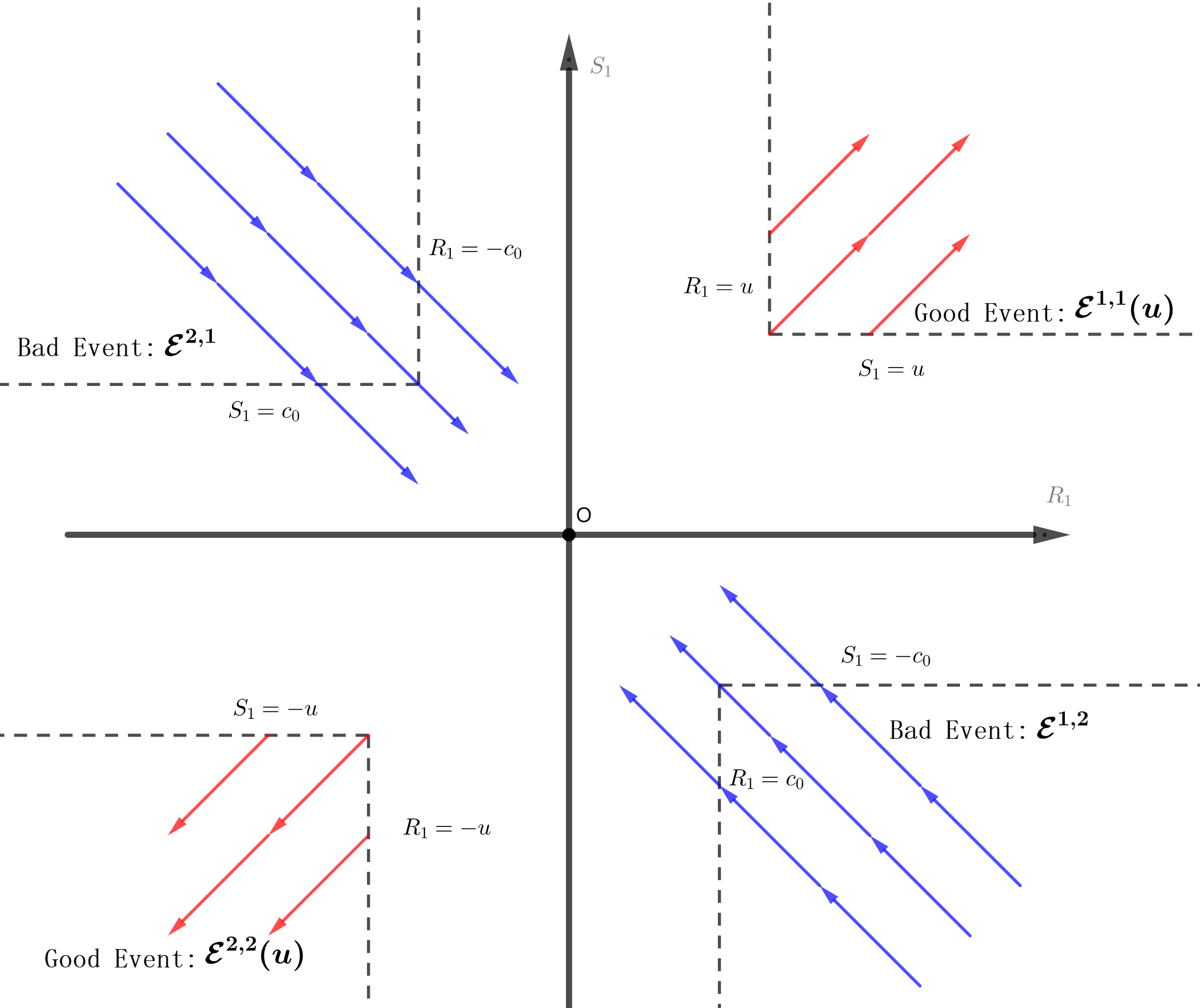
Figure 1: A schematic diagram of behaviors of $R_{1,t}$ and $S_{1,t}$.

Step 1: Choosing ${\text{opt}}_{1},{\text{opt}}_{2}$ with Nonzero Probability

Combining Lemmas 4.2 and 4.3, we have the following Lemma 4.4, which completes step 1.

Lemma 4.4.

Given the game defined in theorem 4.1, for any round $t\geq 0$ and $i\in\{1,2\}$, if $\sum_{j=1}^{t}r_{i,j}\geq 0$, the probability for Alice to choose ${\text{opt}}_{i}$ is larger than $\frac{1}{4}$; if $\sum_{j=1}^{t}s_{i,t}\geq 0$, the probability for Bob to choose ${\text{opt}}_{i}$ is larger than $\frac{1}{4}$.

Step 2: Escaping Bad Events

Before introduce the formal statement of step 2, we define two "bad events". Given $c_{0}$ for all $t\geq 1$ $\mathcal{E}_{t}^{1,2}:=\{R_{1,t}>c_{0},\text{ and }S_{2,t}>c_{0}\}\text{ and }\mathcal{E}_{t}^{2,1}:=\{R_{2,t}>c_{0}\text{ and }S_{1,t}>c_{0}\}$. We will specify $c_{0}$ later. Intuitively, when $c_{0}$ is sufficiently large, $\mathcal{E}_{t}^{1,2}$ implies that Alice and Bob will choose ${\text{opt}}_{1},{\text{opt}}_{2}$ respectively with a probability close to $1$ in following rounds. For simplicity, we treat each event $\mathcal{E}$ as an indicator function, i.e., $\mathcal{E}$ happens if and only if $\mathcal{E}=1$. In order to prove that these two bad events cannot go on forever, we want to show that when $\mathcal{E}_{t}^{1,2}$ happens, $R_{1,t}-R_{2,t}$ will tend to decrease at a rapid rate. Therefore, Alice will eventually deviate from ${\text{opt}}_{1}$ to choose ${\text{opt}}_{2}$ with a relatively high probability.

By LABEL:asm.fullsupf and lemma 4.2, given $\delta>0$ there exists a constant $c_{1}$ such that when $R_{1,t}>c_{1}$, Alice chooses ${\text{opt}}_{1}$ with probability larger than $1-\delta$; when $S_{2,t}>c_{1}$, Bob chooses ${\text{opt}}_{2}$ with probability larger than $1-\delta$. Let $\gamma_{1}=P_{X,Y}(1,1)+P_{X,Y}(0,0)-P_{X,Y}(1,0)-P_{X,Y}(0,1)$ $\gamma_{2}=(P_{X,Y}(1,1)-P_{X,Y}(0,0))^{2}-(P_{X,Y}(1,0)-P_{X,Y}(0,1))^{2}$.

Lemma 4.5.

Given the game defined in theorem 4.1, there exists a $\delta>0$ and corresponding $c_{1}$ such that for any round $t$, $\mathbb{E}[r_{1,t+1}-r_{2,t+1}|S_{1,t-1}>c_{1}+1]\geq\frac{\gamma_{1}-\gamma_{2}}{2}>0.$

Given such $\delta$ and $c_{1}$ in lemma 4.5, we set $c_{0}=c_{1}+\lceil\frac{1000}{\gamma_{1}-\gamma_{2}}\rceil+1$. Because in each round $R_{1,t},R_{2,t}$ and $S_{1,t},S_{2,t}$ vary by at most $1$, if $\mathcal{E}_{t}^{1,2}$ happens Alice chooses ${\text{opt}}_{1}$ and Bob chooses ${\text{opt}}_{2}$ with probability larger than $1-\delta$ independently for the next $\lceil\frac{1000}{\gamma_{1}-\gamma_{2}}\rceil+1$ rounds. Similar argument holds for $\mathcal{E}_{t}^{2,1}$. We use the above observation to show lemma 4.6.

Lemma 4.6.

Given the game defined in theorem 4.1, for all $t$ and history $\mathcal{H}_{t}\in\mathcal{E}_{t}^{1,2}$, we have $\mathbb{E}\left[\sum_{j=1}^{\lceil\frac{1000}{\gamma_{1}-\gamma_{2}}\rceil+1}(r_{1,t+j}-r_{2,t+j})\middle|\mathcal{H}_{t}\right]\leq-100.$

This lemma formalizes the blue arrows in Fig. 1. With this lemma, we get the main result of step two.

Lemma 4.7.

Given the game defined in theorem 4.1, $\Pr\left\{\limsup_{t\rightarrow\infty}\overline{\mathcal{E}_{t}^{1,2}\vee\mathcal{E}_{t}^{2,1}}=1\right\}=1.$

If we treat $R_{1,t}-R_{2,t}$ as money of Alice, Lemma 4.7 is similar to the gambler’s ruin problem [8]. More specifically, $R_{1,t}-R_{2,t}$ has a negative expected growth each $\lceil\frac{1000}{\gamma_{1}-\gamma_{2}}\rceil+1$ rounds by Lemma 4.6, so $R_{1,t}-R_{2,t}$ will always become small enough to escape $\mathcal{E}^{1,2}$.

Step 3: From Intermediate States to Good Events

We define a series of "good events" at first. For all $u\in{\mathbb{N}}^{+}$ and $t\geq 1$, $\mathcal{E}^{1,1}_{t}(u):=\{R_{1,t}\geq u,\text{ and }S_{1,t}\geq u\}\text{ and }\mathcal{E}^{2,2}_{t}(u):=\{R_{2,t}\geq u\text{ and }S_{2,t}\geq u\}$.

To the end, we want to show that $\vee_{t\in\mathbb{N}^{+}}\mathcal{E}^{1,1}_{t}(u)$ and $\vee_{t\in\mathbb{N}^{+}}\mathcal{E}^{2,2}_{t}(u)$ happen with probability $1$ for any $u\in\mathbb{N}^{+}$. Formally, we claim Lemma 4.8.

Lemma 4.8.

Given the game defined in theorem 4.1, for all $u$ there exists $\lambda_{u}$ so that for any $T$ with history $\mathcal{H}_{T}\in\overline{\mathcal{E}_{T}^{1,2}\vee\mathcal{E}_{T}^{2,1}}$, we have $\Pr\left\{\left(\vee_{i=T}^{T+4(u+c_{0})+100}\mathcal{E}^{1,1}_{t}(u)\right)\vee\left(\vee_{i=T}^{T+4(u+c_{0})+100}\mathcal{E}^{2,2}_{t}(u)\right)=1\middle|\mathcal{H}_{T}\right\}\geq\lambda_{u}$.

This lemma generally says that when the agents are in an intermediate state that $\overline{\mathcal{E}_{T}^{1,2}\vee\mathcal{E}_{T}^{2,1}}=1$, they have a constant probability $\lambda_{u}$ to get into a good event in the next $4(u+c_{0})+100$ rounds. In order to prove this lemma, we define a nice event $\mathcal{P}_{T}$ such that $\mathcal{P}_{T}$ happens with probability larger than $\lambda_{u}$ and $\mathcal{P}_{T}$ implies the good events happen in no more than $4(u+c_{0})+100$ rounds. Formally, event $\mathcal{P}_{T}$ is defined as the following: First, for $j=T,\dots,T_{1}$ until some round $T_{1}\geq T$ such that $S_{1,T_{1}}\geq 0$, $x_{j+1}=1-\hat{y}_{j},y_{j+1}=1-\hat{x}_{j}$, Alice uses strategy ${\text{opt}}_{1}$, Bob uses strategy ${\text{opt}}_{2}$. Then, Alice and Bob uses strategy ${\text{opt}}_{1}$ for $4u+50$ rounds and signals are generated as $x_{j+1}=y_{j+1}=-x_{j}$ for $j\geq T_{1}$. We can use Lemma 4.4 to prove that $\lambda_{u}=(\min_{i,j\in\{0,1\}}\{P_{X,Y}(i,j)\}\times 0.25^{2})^{100+4(u+c_{0})}$ is a feasible lower bound.

Step 4: Good Events Lead to Truthful Convergence

Similar to step 2, we have lemma 4.9 to show that $\mathcal{E}_{t}^{1,1}(u)$ can lead to increasing of $R_{1,t}-R_{2,t}$ at first. The idea is completely similar to Lemma 4.6 and it formalize the red arrows in Fig. 1.

Lemma 4.9.

Given the game defined in theorem 4.1, for all $u>2c_{0}+1$ and $t$ if $\mathcal{H}_{t}\in\mathcal{E}_{t}^{1,1}\left(\lfloor\frac{u}{2}\rfloor\right)$, we have $\mathbb{E}\left[\sum_{j=1}^{\lceil\frac{1000}{\gamma_{1}-\gamma_{2}}\rceil+1}\left(r_{1,t+j}-r_{2,t+j}\right)\middle|\mathcal{H}_{t}\right]\geq 100$.

Using Lemma 4.9, we are able to prove that for any $\varepsilon$, there exists a $u$ such that when $\mathcal{E}_{t}^{1,1}(u)$ or $\mathcal{E}_{t}^{2,2}(u)$ happens, Alice and Bob will tend to choose $({\text{opt}}_{1},{\text{opt}}_{1})$ or $({\text{opt}}_{2},{\text{opt}}_{2})$ with increasingly higher probability. Formally, we propose Lemma 4.10.

Lemma 4.10.

Given the game defined in theorem 4.1, for all $\epsilon>0$ there exists $u\in\mathbb{N}^{+}$ such that given a history $\mathcal{H}_{T}\in\mathcal{E}_{T}^{1,1}(u)\vee\mathcal{E}_{T}^{2,2}(u)$, we have $\Pr\left\{\forall i\in\mathbb{N},\mathcal{E}_{T+\left(\lceil\frac{1000}{\gamma_{1}-\gamma_{2}}\rceil+1\right)i}^{1,1}\left(\lfloor\frac{u}{2}\rfloor+i\right)\vee\mathcal{E}_{T+\left(\lceil\frac{1000}{\gamma_{1}-\gamma_{2}}\rceil+1\right)i}^{2,2}\left(\lfloor\frac{u}{2}\rfloor+i\right)=1\middle|\mathcal{H}_{T}\right\}\geq 1-\varepsilon$.

We design a sub-martingale $\{D_{i}\}_{i\in\mathbb{N}}$ that is proportional to $R_{1,T+i\left(\lceil\frac{1000}{\gamma_{1}-\gamma_{2}}\rceil+1\right)}-R_{2,T+i\left(\lceil\frac{1000}{\gamma_{1}-\gamma_{2}}\rceil+1\right)}$, and use Azuma-Hoeffding inequality to prove lemma 4.10.

5 Simulations

We simulate the CA mechanism with various learning algorithms: the Hedge algorithms, follow the perturbed leader, follow the leader, and $\epsilon$-greedy, and repeat the process 400 times with 800 rounds on each algorithm each time. We define the converge proportion in round $t$ as the fraction of the simulations where both agents report truthfully ${\text{opt}}_{1}$ (or both use ${\text{opt}}_{2}$) in all the subsequent rounds.

In our simulations, we use the following private signal distribution that satisfies LABEL:asm.poscorr: $P_{X,Y}(0,0)=P_{X,Y}(1,1)=0.4,P_{X,Y}(1,0)=P_{X,Y}(0,1)=0.2$. Moreover, Alice and Bob are using the same learning algorithms in our simulations that are listed below: First, Follow the Leader algorithm (FTL) chooses ${\text{opt}}_{i}$ with probability proportional to $\mathbb{I}[R_{i}=\max\{R_{1},R_{2},R_{3},R_{4}\}]$. Follow the perturbed leader (FPL*, where * can be 1, 4 or 8) adds a uniform random noise between $0$ and $*$ and choose strategy ${\text{opt}}_{i}$ with probability $\Pr\left\{R_{i}+p_{i}=\max_{j\in[4]}\{R_{j}+p_{j}\}\middle|p_{j}\overset{\mathrm{iid}}{\sim}\mathcal{U}[0,*]\right\}$. We consider FPL1, FPL4, and FPL8. Hedge algorithm 1 choose $i$ with probability proportional to $3^{R_{i}/2}$ that is an implementation by choosing $\epsilon=0.5$ for the multiplicative weights algorithm of Arora et al. [2]. Hedge algorithm 2 chooses $i$ with probability proportional to $e^{R_{i}}$ that is an implementation by choosing $\beta=1$ of exponentially weighted averaged forecaster introduced by Freund and Schapire [11]. Finally, $\epsilon$-greedy algorithm uses time varying $\epsilon=\frac{1}{(t+1)^{2}}$ at round $t$. Note that $\epsilon$-greedy is not in $\mathcal{A}$ but still achieves truthful convergence.

In Figure 2, all our algorithms converge to truth-telling. First, all reward-based online learning algorithms (the Hedge algorithms, follow the perturbed leader, and follow the leader) exhibit truthful convergence that aligns with our theoretical result, theorem 4.1. Moreover, although FTL is generally not no-regret, CA mechanism still works well with it. Additionally, we observe that when an algorithm explores less (e.g. FPL4 vs FPL8), it converges faster, but very little exploration does not further improve the convergence rate (e.g. FTL vs FPL2). Finally, we also find that the $\epsilon$-greedy with time decreasing $\epsilon$, which is not a reward-based online learning algorithm, also shows truthful convergence. This suggests that the CA mechanism may have truthful convergence beyond reward-based online learning algorithms.

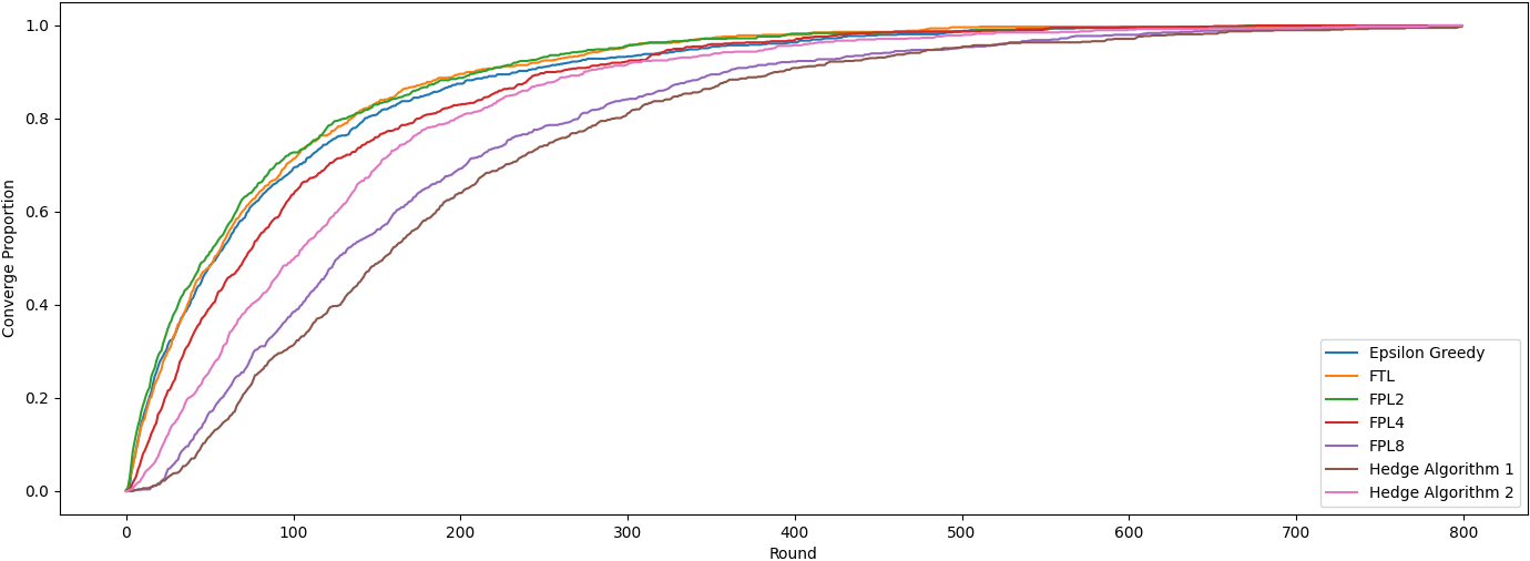
Figure 2: Convergence Rates of Learning Algorithms in CA.

6 Conclusions

In this paper, we study sequential peer prediction with learning agents and prove that the notion of no-regret alone is not sufficient for truthful convergence. We then define a family of reward-based learning algorithms and show that the CA mechanism is able to achieve truthful convergence when agents use algorithms in this family. Finally, we give a discussion on the converge rates of different learning agents based on simulations.

This is the first theoretical study on peer prediction with learning agents. There are many open problems and future directions to extend this work. We believe similar proof techniques can be used to extend our results to settings where agents’ private signals are generated by a Markov chain with some assumptions on the transition matrix. Moreover, this work is only restricted to binary signals and it is still an open problem whether there exists a mechanism for non-binary settings that can promise truthful convergence. For the learning agents, one could consider a more general family of learning algorithms such as when $f$ is time-varying.

Appendix

Appendix A Basic Math

A.1 Martingale and Concentration

In this section we will define martingales and some of its properties.

Definition A.1 (Martingale).

Let $\mathcal{F}=\{\mathcal{F}_{t}\}_{t\in\mathbb{N}}$ be a filtration, which is an increasing sequence of $\sigma$-field. A martingale with respect to $\mathcal{F}$ is a sequence $D_{0},D_{1},D_{2},\cdots$ adapted to $\mathcal{F}$ ($D_{t}\in\mathcal{F}_{t}$ for all $t$) that satisfies for any time $t$,

$$\mathbb{E}\left[|D_{t}|\right]<\infty,$$

$$\mathbb{E}\left[D_{t+1}|\mathcal{F}_{t}\right]=D_{t}.$$

There are two extensions of a martingale that replace the equality of conditional probability by upper and lower bounds.

Definition A.2 (Sub-martingale and super-martingale).

Let $\mathcal{F}=\{\mathcal{F}_{t}\}_{t\in\mathbb{N}}$ be a filtration, which is an increasing sequence of $\sigma$-field. A sub-martingale with respect to $\mathcal{F}$ is a sequence $D_{0},D_{1},D_{2},\cdots$ adapted to $\mathcal{F}$ that satisfies for any time $t$,

$$\mathbb{E}\left[|D_{t}|\right]<\infty,$$

$$\mathbb{E}\left[D_{t+1}|\mathcal{F}_{t}\right]\geq D_{t}.$$

A super-martingale with respect to $\mathcal{F}$ is a sequence $D_{0},D_{1},D_{2},\cdots$ adapted to $\mathcal{F}$ that satisfies for any time $t$,

$$\mathbb{E}\left[|D_{t}|\right]<\infty,$$

$$\mathbb{E}\left[D_{t+1}|\mathcal{F}_{t}\right]\leq D_{t}.$$

For a sub-martingale (or super-martingale), we have the Azuma–Hoeffding inequality [1], which is a concentration result for the values of martingales.

Theorem A.3 (name = Azuma–Hoeffding inequality, label = thm:asuma).

Suppose $\{D_{t}\}_{t\in\mathbb{N}}$ is a martingale (or super-martingale) and $|D_{t}-D_{t-1}|\leq c_{t}$ almost surely. Then for any $T\in\mathbb{N}^{+}$ and $\epsilon\in\mathbb{R}^{+}$, we have

$$\Pr\left\{D_{t}-D_{0}\geq\epsilon\right\}\leq\exp\left(\frac{-\epsilon^{2}}{2\sum_{t=1}^{T}c_{t}^{2}}\right).$$

And symmetrically, if $\{D_{t}\}_{t\in\mathbb{N}}$ is a sub-martingale, we have

$$\Pr\left\{D_{t}-D_{0}\leq-\epsilon\right\}\leq\exp\left(\frac{-\epsilon^{2}}{2\sum_{t=1}^{T}c_{t}^{2}}\right).$$

Now we define stopping time. This is intuitively a condition such that the "decision" whether to stop in the $t^{th}$ round should be based on information of the first $t$ rounds, instead of any future information.

Definition A.4 (Stopping time).

$\tau$ is called a stopping time for a filtration $\mathcal{F}$ if and only if $\{\tau=t\}\in\mathcal{F}_{t},\forall t$.

A.2 Limit Inferior and Limit Superior

Limit inferior and limit superior are defined on sequences, representing limit bounds of a sequence. To meet our needs, our definition focus on discrete metric.

Definition A.5.

Let $\{\mathcal{E}_{t}\}_{t\in\mathbb{N}^{+}}$ be a sequence of events. Limit inferior and limit superior of this sequence are

$$\liminf_{t\rightarrow+\infty}\mathcal{E}_{t}=\vee_{t=1}^{+\infty}\left(\wedge_{i=t}^{+\infty}\mathcal{E}_{i}\right),$$

and

$$\limsup_{t\rightarrow+\infty}\mathcal{E}_{t}=\wedge_{t=1}^{+\infty}\left(\vee_{i=t}^{+\infty}\mathcal{E}_{i}\right).$$

A.3 Borel-Cantelli Lemma

In this section, we formally introduce Borel-Cantelli lemma. Its proof can be found in [10].

Theorem A.6 (Borel-Cantelli lemma).

Let $\mathcal{E}_{1},\mathcal{E}_{2},\cdots$ be a sequence of events in some probability space. Borel-Cantelli lemma states that if $\sum_{t=1}^{+\infty}\Pr\{\mathcal{E}_{t}\}<\infty$, then the probability that infinitely many of $\mathcal{E}_{t}$’s occur is $0$, or more strictly,

$$\Pr\left\{\limsup_{t\rightarrow+\infty}\mathcal{E}_{t}\right\}=0.$$

Appendix B Truthfulness of CA mechanism for Bayesian Agents

In this section, we assume that both agents are using consistent strategies as previous works assume [5, 26, 18, 24, 16, 29]. The formal definition of consistent strategy is given in LABEL:def.consist.

Definition B.1 (name = Consistent strategy, label = def.consist).

In a repeated game, a strategy profile $\sigma$ is a consistent strategy if and only if for each agent $i$, she adopts $\sigma_{i}$ identically over each round of the game.

In a sequential peer prediction game, for agent $i$, we set the average payoffs of agent $i$ in $T$ rounds as her utility.

Then we introduce Bayesian Nash equilibrium. A Bayesian Nash equilibrium (BNE) is strategies of agents that have the maximal expected payoff for each player given their beliefs on environments and others’ strategies [13].

Definition B.2 (Bayesian Nash equilibiurm).

A strategy profile $\sigma$ is a Bayesian Nash equilibrium if and only if for every agent $i$, the expected payoff of using $\sigma_{i}$ for agent $i$ is maximal keeping other agents’ strategies unchanged. Moreover, A strategy profile $\sigma$ is a strict Bayesian Nash equilibrium if and only if for every agent $i$, the expected payoff of using $\sigma_{i}$ for agent $i$ is strictly larger than any other strategies keeping other agents’ strategies unchanged.

Moreover, We say a peer prediction mechanism is strongly truthful if agents in truthtelling equilibrium get strictly higher payment than any other non-permutation equilibrium [26]. Here, a permutation equilibrium is the strategy profile that agents report a permutation of the signal. Formally, we have definition B.3.

Definition B.3 (Strongly truthful).

In a peer prediction game, if agents are using consistent strategies, a mechanism is strongly truthful if and only if truthtelling is a BNE and also guarantees larger agent welfare than any non-permutation equilibrium. Here, welfare is defined by each agent’s expected payoff so that is to say, the expected payoff of each agent using truthtelling strategy profile is strictly higher than the expected payoff using non-permutation equilibrium.

Though Dasgupta and Ghosh [5], Shnayder et al. [26] have proved that CA mechanism is strongly truthful in non-sequential settings, our settings are slightly different from theirs and we rewrite the proof for binary sequential peer prediction settings. More specifically, our CA mechanism uses the last round agreement term instead of average agreement term in the payoffs and we are focusing on average payoffs instead of total payoffs. Before the complete proof, we have the following lemma.

Lemma B.4.

For binary sequential signal peer prediction games under LABEL:asm.apriori and LABEL:asm.poscorr, if both agents are using consistent strategies, CA mechanism renders truthtelling strategy profile a strict Bayesian Nash equilibrium.

Proof.

We know that Alice and Bob are Bayesian agents using consistent strategies. Then we can suppose when Alice gets signal $1$, she reports $1$ with probability $p_{1}$; when she gets signal $0$, she reports $0$ with probability $p_{0}$. Similarly, Bob is using a fixed strategy that when he gets signal $1$, he reports $1$ with probability $q_{1}$; when he gets signal $0$, he reports $0$ with probability $q_{0}$. Therefore, we can compute the first term in payoff of Alice and Bob (see eq. 1), $\mathbb{E}[\mathbb{I}[\hat{x}_{t}=\hat{y}_{t}]]$, by

$$\mathbb{E}[\mathbb{I}[\hat{x}_{t}=\hat{y}_{t}]] =P_{X,Y}(1,1)(p_{1}q_{1}+(1-p_{1})(1-q_{1}))+P_{X,Y}(0,0)(p_{0}q_{0}+(1-p_{0})(1-q_{0}))$$

$$+P_{X,Y}(1,0)(p_{1}(1-q_{0})+(1-p_{1})q_{0})+P_{X,Y}(0,1)(q_{1}(1-p_{0})+(1-q_{1})p_{0}).$$

Also, we can compute the second term

$$\mathbb{E}[\mathbb{I}[\hat{x}_{t}=\hat{y}_{t-1}]] =(P_{X,Y}(1,1)+P_{X,Y}(1,0))(P_{X,Y}(0,1)+P_{X,Y}(1,1))(p_{1}q_{1}+(1-p_{1})(1-q_{1}))$$

$$+(P_{X,Y}(0,0)+P_{X,Y}(0,1))(P_{X,Y}(1,0)+P_{X,Y}(0,0))(p_{0}q_{0}+(1-p_{0})(1-q_{0}))$$

$$+(P_{X,Y}(1,1)+P_{X,Y}(1,0))(P_{X,Y}(0,0)+P_{X,Y}(1,0))(p_{1}(1-q_{0})+(1-p_{1})q_{0})$$

$$+(P_{X,Y}(0,1)+P_{X,Y}(0,0))(P_{X,Y}(0,1)+P_{X,Y}(1,1))((1-p_{0})q_{1}+p_{0}(1-q_{1})).$$

Similarly, $\mathbb{E}[\mathbb{I}[\hat{y}_{t}=\hat{x}_{t-1}]]$ also equals to this expression.

To prove BNE, we only need to prove that when $q_{0}=q_{1}=1$, we have

$$\operatorname*{arg\,max}_{(p_{0},p_{1})}\left\{\mathbb{E}[\mathbb{I}[\hat{x}_{t}=\hat{y}_{t}]]-\mathbb{E}[\mathbb{I}[\hat{x}_{t}=\hat{y}_{t-1}]]\right\}=(1,1).$$ (2)

The other side when $p_{0}=p_{1}=1$ is symmetrical.

Actually, we have

$$\frac{\partial(\mathbb{E}[\mathbb{I}[\hat{x}_{t}=\hat{y}_{t}]|q_{0}=q_{1}=1]-\mathbb{E}[\mathbb{I}[\hat{x}_{t}=\hat{y}_{t-1}]|q_{0}=q_{1}=1])}{\partial p_{0}}$$

$$=P_{X,Y}(0,0)-P_{X,Y}(0,1)$$

$$+(P_{X,Y}(0,0)+P_{X,Y}(0,1))(P_{X,Y}(0,1)+P_{X,Y}(1,1)-P_{X,Y}(0,0)-P_{X,Y}(1,0))$$

$$=2P_{X,Y}(0,0)-2(P_{X,Y}(0,0)+P_{X,Y}(0,1))(P_{X,Y}(0,0)+P_{X,Y}(1,0))$$

$$=2(P_{X,Y}(0,0)P_{X,Y}(1,1)-P_{X,Y}(0,1)P_{X,Y}(1,0))$$

$$>0,$$

and

$$\frac{\partial(\mathbb{E}[\mathbb{I}[\hat{x}_{t}=\hat{y}_{t}]|q_{0}=q_{1}=1]-\mathbb{E}[\mathbb{I}[\hat{x}_{t}=\hat{y}_{t-1}]|q_{0}=q_{1}=1])}{\partial p_{1}}$$

$$=P_{X,Y}(1,1)-P_{X,Y}(1,0)$$

$$+(P_{X,Y}(1,1)+P_{X,Y}(1,0))(P_{X,Y}(0,0)+P_{X,Y}(1,0)-P_{X,Y}(1,1)-P_{X,Y}(0,1))$$

$$=2P_{X,Y}(1,1)-2(P_{X,Y}(1,1)+P_{X,Y}(1,0))(P_{X,Y}(1,1)+P_{X,Y}(0,1))$$

$$=2(P_{X,Y}(1,1)P_{X,Y}(0,0)-P_{X,Y}(0,1)P_{X,Y}(1,0))$$

$$>0,$$

which indicate eq. 2. ∎

Furthermore, we can find all the Nash equilibria for Bayesian agents under our CA mechanism in sequential peer prediction setting. We have theorem B.5.

Theorem B.5.

For binary sequential signal peer prediction games under LABEL:asm.apriori and LABEL:asm.poscorr, if CA mechanism is used and agents adopt consistent strategies, there are three types of Nash equilibria for agents, which are

1. truth-telling ${\text{opt}}_{1}$,

2. flip the signal ${\text{opt}}_{2}$,

3. report regardless of private signals (uninformative reports).

Proof.

Using the same notations in the proof of lemma B.4, we deduce that

$$\frac{\partial(\mathbb{E}[\mathbb{I}[\hat{x}_{t}=\hat{y}_{t}]]-\mathbb{E}[\mathbb{I}[\hat{x}_{t}=\hat{y}_{t-1}]])}{\partial p_{0}}$$

$$=(P_{X,Y}(1,1)P_{X,Y}(0,0)-P_{X,Y}(1,0)P_{X,Y}(0,1))(2q_{0}+2q_{1})$$

$$-2(P_{X,Y}(1,1)P_{X,Y}(0,0)-P_{X,Y}(1,0)P_{X,Y}(0,1)),$$

and similarly,

$$\frac{\partial(\mathbb{E}[\mathbb{I}[\hat{x}_{t}=\hat{y}_{t}]]-\mathbb{E}[\mathbb{I}[\hat{x}_{t}=\hat{y}_{t-1}]])}{\partial p_{1}}$$

$$=(P_{X,Y}(1,1)P_{X,Y}(0,0)-P_{X,Y}(1,0)P_{X,Y}(0,1))(2q_{0}+2q_{1})$$

$$-(P_{X,Y}(1,1)P_{X,Y}(0,0)-P_{X,Y}(1,0)P_{X,Y}(0,1)).$$

Therefore, we know that when $q_{0}+q_{1}>1$, the best response of Alice is $p_{0}=p_{1}=1$; when $q_{0}+q_{1}<1$, the best response of Alice is $p_{0}=p_{1}=0$. Symmetrically, we can deduce that when $p_{0}+p_{1}>1$, the best response of Alice is $q_{0}=q_{1}=1$; when $p_{0}+p_{1}<1$, the best response of Alice is $q_{0}=q_{1}=0$.

Let $p_{0}^{*},p_{1}^{*},q_{0}^{*},q_{1}^{*}$ be a Nash equilibrium for this peer prediction game under CA mechanism. Then given $p_{0}^{*},p_{1}^{*}$, $q_{0}^{*},q_{1}^{*}$ should be one of the best responses of Bob; given $q_{0}^{*},q_{1}^{*}$, $p_{0}^{*},p_{1}^{*}$ should be one of the best responses of Alice.

If $p_{0}^{*}+p_{1}^{*}>1$, then the only best response of Bob is $q_{0}=q_{1}=1$, so $q^{*}_{0}=q^{*}_{1}=1$. When $q^{*}_{0}=q^{*}_{1}=1$, the only best response of Alice is $p_{0}=p_{1}=1$, so we can deduce that $p_{0}^{*}=p_{1}^{*}=q_{0}^{*}=q_{1}^{*}=1$ is the unique Nash equilibrium for this case.

If $p_{0}^{*}+p_{1}^{*}<1$, then the only best response of Bob is $q_{0}=q_{1}=0$, so $q^{*}_{0}=q^{*}_{1}=0$. When $q^{*}_{0}=q^{*}_{1}=0$, the only best response of Alice is $p_{0}=p_{1}=0$, so we can deduce that $p_{0}^{*}=p_{1}^{*}=q_{0}^{*}=q_{1}^{*}=0$ is the unique Nash equilibrium for this case.

Symmetrically, when $q_{0}^{*}+q_{1}^{*}\neq 1$, there are still only these two Nash equilibria. Moreover, it is easy to verify that $p_{0}^{*},p_{1}^{*},q_{0}^{*},q_{1}^{*}$ that satisfies $p_{0}^{*}+p_{1}^{*}=q_{0}^{*}+q_{1}^{*}=1$ is Nash equilibrium. Therefore, all the uninformative reports are Nash equilibria. These are exactly what we want to prove. ∎

From the proof of lemma B.4, we can observe that when both agents use ${\text{opt}}_{1}$, their expected payoffs are both

$$P_{X,Y}(1,1)+P_{X,Y}(0,0)-(P_{X,Y}(1,1)+P_{X,Y}(1,0))(P_{X,Y}(0,1)+P_{X,Y}(1,1))$$

$$-(P_{X,Y}(0,1)+P_{X,Y}(0,0))(P_{X,Y}(1,0)+P_{X,Y}(0,0))$$

$$=2P_{X,Y}(1,1)P_{X,Y}(0,0)-2P_{X,Y}(1,0)P_{X,Y}(0,1)$$

$$>0.$$

Also, we can observe that when both agents use uninformative reports, their expected payoffs are both $0$. According to theorem B.5, we know that the only non-permutation equilibrium is uninformative reports. Therefore, we deduce that CA mechanism is strongly truthful.

Theorem B.6.

For binary sequential signal peer prediction games under LABEL:asm.apriori and LABEL:asm.poscorr, if agents adopt consistent strategies, CA mechanism is strongly truthful.

Appendix C Proofs and Details of Section 3.1

C.1 Impossibility of Truthful Convergence for No Regret Agents

Proof of LABEL:thm:impossible.

First, for any sequential information elicitation mechanism because Alice and Bob can use arbitrary no regret algorithm, there exist no-regret for Alice and Bob. If the truth-telling has regret on $\mathcal{M}$, the statement trivially holds. Otherwise, suppose truth-telling is no regret on $\mathcal{M}$. We have for all $T$ the expectations $\mu^{X}_{T}=\max_{i}\sum_{t\leq T}\mathbb{E}r_{i,t}-\sum_{t\leq T}\mathbb{E}r_{t}$ and $\mu^{Y}_{T}=\max_{i}\sum_{t\leq T}\mathbb{E}s_{i,t}-\sum_{t\leq T}\mathbb{E}s_{t}$ satisfy

$$\mu_{T}^{X}\text{ and }\mu_{T}^{Y}=o(T).$$ (3)

We will use probabilistic method to show the existence of a deterministic and no regret sequence of strategies $({\text{opt}}^{X}_{t},{\text{opt}}^{Y}_{t})_{t=1,\dots}$ that consists of reporting $1$ and $0$ regardless of private signal ${\text{opt}}_{3},{\text{opt}}_{4}$. As a result, when Alice and Bob use the sequence, the algorithm is no regret but $\mathcal{M}$ does not achieve truthful convergence on such algorithm. To find such sequence, it is sufficient for us to find a deterministic sequence $(\hat{x}^{*}_{t},\hat{y}^{*}_{t})_{t\geq 1}$ so that for all $T$

$$\max_{i}\sum r^{*}_{i,t}-\sum r^{*}_{t}\text{ and }\max_{i}\sum s^{*}_{i,t}-\sum s^{*}_{t}=o(T),$$ (4)

because we can define an online learning algorithms so that Alice play ${\text{opt}}^{X}_{t}={\text{opt}}_{2+\hat{x}_{t}^{*}}$ and Bob play ${\text{opt}}^{Y}_{t}={\text{opt}}_{2+\hat{y}^{*}_{t}}$ for all $t$. Additionally, if we can find $(\hat{{\mathbf{x}}}^{*}_{t},\hat{{\mathbf{y}}}^{*}_{t})_{1\leq t}$ and $T_{0}$ that for all $T\geq T_{0}$,

$$|\max_{i}\sum r_{i,t}-\sum r_{t}-\mu^{X}_{T}|\text{ and }|\max_{i}\sum s_{i,t}-\sum s_{t}-\mu^{Y}_{T}|\leq T^{2/3},$$ (5)

by eq. 3 $(\hat{{\mathbf{x}}}^{*}_{t},\hat{{\mathbf{y}}}^{*}_{t})_{1\leq t}$ satisfies eq. 4.

Because their signal mutually independent across different rounds and each round’s signals can only affect at most $2k-1$ rounds of payoff, each pair of signals only changes $\max_{i}\sum_{t\leq T}r_{i,t}-\sum_{t\leq T}r_{t}$ by $2(2k-1)\leq 4k$. Therefore, by Chernoff bound using method of bounded difference, we have for all $T$ and $\epsilon>0$

$$\Pr\left[\left|\max_{i}\sum_{t\leq T}r_{i,t}-\sum_{t\leq T}r_{t}-\mu_{T}^{X}\right|\leq\epsilon T\right]\leq 2\exp\left(-\frac{2\epsilon^{2}}{16k^{2}}T\right)$$

$$\Pr\left[\left|\max_{i}\sum_{t\leq T}s_{i,t}-\sum_{t\leq T}s_{t}-\mu_{T}^{Y}\right|\leq\epsilon T\right]\leq 2\exp\left(-\frac{2\epsilon^{2}}{16k^{2}}T\right)$$

Thus, we can take $\epsilon=T^{-1/3}$ and $T_{0}$ large enough and prove the random payoffs of truth-telling satisfy eq. 5 for all $T\geq T_{0}$ with high probability by union bound. Therefore, by probabilistic method there exists a (determistic) sequence $(\hat{{\mathbf{x}}}^{*}_{t},\hat{{\mathbf{y}}}^{*}_{t})_{1\leq t}$ so that eq. 5 holds for all $T\geq T_{0}$. ∎

C.2 Truthful Convergence Implies No regret

Proof of LABEL:thm:converge2noregret.

Given reports $\hat{{\mathbf{x}}}$ and signals ${\mathbf{x}}$, let $\hat{{\mathbf{x}}}_{t-k:t}=(\hat{x}_{t-k+1},\dots,\hat{x}_{t})$ be a slice of reports $\hat{{\mathbf{x}}}$, and ${\text{opt}}_{i}({{\mathbf{x}}}_{t-k:t})=({\text{opt}}_{i}(x_{t-k+1}),\dots,{\text{opt}}_{i}(x_{t}))$ be a slice reports under consistent strategy ${\text{opt}}_{i}$. Given $T$, we define four functions on the signals

$$F^{i}_{T}({\mathbf{x}},{\mathbf{y}}):=\sum_{t=0}^{T}\bar{M}^{X}({\text{opt}}_{i}({\mathbf{x}}_{t-k:t}),{{\mathbf{y}}}_{t-k:t})-\bar{M}^{X}({{\mathbf{x}}}_{t-k:t},{{\mathbf{y}}}_{t-k:t})$$

for $i=1,2,3,4$. We want to show the value of $F^{i}_{T}$ is small. Specifically, we bound the probability of the following good event

$$\mathcal{G}:=\{\max_{i}F^{i}_{T}({\mathbf{x}},{\mathbf{y}})\leq T^{2/3}\}.$$

First because $\bar{M}$ is strongly truthful, $\mathbb{E}_{\sigma^{X}}[\bar{M}^{X}(\hat{{\mathbf{x}}},{\mathbf{y}})]\leq\mathbb{E}[\bar{M}^{X}({{\mathbf{x}}},{\mathbf{y}})]$ and $\mathbb{E}_{\sigma^{Y}}[\bar{M}^{Y}({{\mathbf{x}}},\hat{{\mathbf{y}}})]\leq\mathbb{E}[\bar{M}^{Y}({{\mathbf{x}}},{\mathbf{y}})]$, the expectation is non-positive

$$\mathbb{E}[F^{i}_{T}({\mathbf{x}},{\mathbf{y}})]=\sum_{t=0}^{T}\mathbb{E}_{\sigma^{X}={\text{opt}}_{i}}\left[\bar{M}^{X}(\hat{{\mathbf{x}}}_{t-k:t},{{\mathbf{y}}}_{t-k:t})-\bar{M}^{X}({{\mathbf{x}}}_{t-k:t},{{\mathbf{y}}}_{t-k:t})\right]\leq 0$$

for all $i$. Second, because each round’s signals are mutually independent and can only affect at most $2k-1$ round of payoff, by Chernoff bound on $F^{i}_{T}$, we have for all $i$, $\Pr\left[F^{i}_{T}({\mathbf{x}},{\mathbf{y}})\geq T^{2/3}\right]\leq\Pr\left[F^{i}_{T}({\mathbf{x}},{\mathbf{y}})\geq T^{2/3}+\mathbb{E}F^{i}_{T}\right]\leq\exp\left(-\frac{2}{16k^{2}}T^{1/3}\right)$. By union bound, we have

$$\Pr\left[\mathcal{G}\right]\geq 1-4\exp\left(-\frac{2}{16k^{2}}T^{1/3}\right).$$ (6)

On the other hand, the truthful convergence consists of two disjoint events: both converging to truth telling ${\text{opt}}_{1}$, and both converging to the flipping strategy ${\text{opt}}_{2}$. By symmetric suppose the first event happens with a nonzero probability

$$\mathcal{E}:=\{\lim_{t\rightarrow+\infty}{\text{opt}}^{X}_{t}=\lim_{t\rightarrow+\infty}{\text{opt}}^{Y}_{t}={\text{opt}}_{1}\}.$$

Then there exists a random round $t^{*}$ so that ${\text{opt}}^{X}_{t}={\text{opt}}^{Y}_{t}={\text{opt}}_{1}$ for all $t\geq t^{*}$ given $\mathcal{E}$. To bound the expected regret conditional on $\mathcal{E}$, we consider two cases: If the converge time $t^{*}$ is greater than $T^{2/3}$, we use the truthful convergence to show the probability is small. Otherwise if the converge time $t^{*}$ is smaller than $T^{2/3}$, we can ignore the first term.

Formally, Alice’s expected regret is

$$\mathbb{E}\left[Reg^{X}(T)\mid\mathcal{E}\right]=\mathbb{E}\left[\mathbf{1}[t^{*}>T^{2/3}]Reg^{X}(T)\mid\mathcal{E}\right]+\mathbb{E}\left[\mathbf{1}[t^{*}\leq T^{2/3}]Reg^{X}(T)\mid\mathcal{E}\right].$$

For the first term, $\mathbb{E}\left[\mathbf{1}[t^{*}>T^{2/3}]Reg^{X}(T)\mid\mathcal{E}\right]\leq T\mathbb{E}\left[\mathbf{1}[t^{*}>T^{2/3}]\mid\mathcal{E}\right]=T\Pr[t^{*}>T^{2/3}\mid\mathcal{E}]$. Because $\Pr[t^{*}>T^{2/3}]=o(1)$ as $T$ increases due to truthful convergence, and $\mathcal{E}$ happens with nonzero probability, we have

$$\mathbb{E}\left[\mathbf{1}[t^{*}>T^{2/3}]Reg^{X}(T)\mid\mathcal{E}\right]=o(T).$$ (7)

On the other hand, when $t^{*}\leq T^{2/3}$ happens,

$$Reg^{X}(T)=\max_{i}\sum_{t\leq T}r_{i,t}-\sum_{t\leq T}r_{t}$$

$$\leq (t^{*}+k)+\max_{i}\sum_{t=t^{*}+k}^{T}r_{i,t}-r_{t} r_{t} r_{i,t} [0,1]$$ ( and are in )

$$= (t^{*}+k)+\max_{i}\sum_{t=t^{*}+k}^{T}\bar{M}^{X}({\text{opt}}_{i}({\mathbf{x}}_{t-k:t}),{{\mathbf{y}}}_{t-k:t})-\bar{M}^{X}({{\mathbf{x}}}_{t-k:t},{{\mathbf{y}}}_{t-k:t}) \mathcal{E}$$ ( happens)

$$\leq 2(t^{*}+k)+\max_{i}F^{i}_{T}({\mathbf{x}},{\mathbf{y}}) t^{*}+k$$ (adding addition terms)

$$\leq 2(T^{2/3}+k)+\max_{i}F^{i}_{T}({\mathbf{x}},{\mathbf{y}}) t^{*}\leq T^{2/3}$$ ()

Therefore,

$$\mathbb{E}\left[\mathbf{1}[t^{*}\leq T^{2/3}]Reg^{X}(T)\mid\mathcal{E}\right]\leq 2(T^{2/3}+k)+\mathbb{E}\left[\max_{i}F^{i}_{T}({\mathbf{x}},{\mathbf{y}})\mid\mathcal{E}\right].$$ (8)

To bound the second term, we partition the expectation by whether $\mathcal{G}$ happens or not

$$\mathbb{E}\left[\max_{i}F^{i}_{T}({\mathbf{x}},{\mathbf{y}})\mid\mathcal{E}\right]$$

$$= \mathbb{E}\left[\max_{i}F^{i}_{T}({\mathbf{x}},{\mathbf{y}})\mid\mathcal{E},\mathcal{G}\right]\Pr[\mathcal{G}\mid\mathcal{E}]+\mathbb{E}\left[\max_{i}F^{i}_{T}({\mathbf{x}},{\mathbf{y}})\mid\mathcal{E},\neg\mathcal{G}\right]\Pr[\neg\mathcal{G}\mid\mathcal{E}]$$

$$\leq T^{2/3}\Pr[\mathcal{G}\mid\mathcal{E}]+T\Pr[\neg\mathcal{G}\mid\mathcal{E}] \mathcal{G}$$ (definition of )

$$\leq T^{2/3}+T\frac{\Pr[\neg\mathcal{G}]}{\Pr[\mathcal{E}]}=O(T^{2/3})$$ (by eq. 6)

Therefore, with eqs. 7 and 8 we show $\mathbb{E}\left[Reg^{X}(T)\mid\mathcal{E}\right]=o(T)+2(T^{2/3}+k)+O(T^{2/3})=o(T)$ that completes the proof. ∎

Appendix D Justifications of Reward-Based Online Learning Algorithm Family $\mathcal{A}$

In this section, we have two subsections to give justifications for learning algorithm family $\mathcal{A}$. In the first part, we introduce two common used learning algorithms and show that they are both reward-based online learning algorithms. The second part gives justifications for LABEL:asm.fullsupf.

D.1 Learning Algorithms in $\mathcal{A}$

In this section, we do not focus on peer prediction problems but consider learning algorithms used on general online decision problems.

D.1.1 Follow the Perturbed Leader

FPL algorithm is designed by [14]. In their work, they have proved that FPL algorithm achieves no best-in-hindsight regret in full-information online decision problems. For simplicity, we consider FPL using on online decision problem with four options ${\text{opt}}_{i},i\in[4]$ in total. The algorithm let the agent choose an arbitrary option among $\operatorname*{arg\,max}_{{\text{opt}}_{i}\in\{{\text{opt}}_{1},{\text{opt}}_{2},{\text{opt}}_{3},{\text{opt}}_{4}\}}(R_{i,t-1}+p_{i,t})$ in the $t^{th}$ round of the game. Here, $p_{i,t}$’s are i.i.d. sampled from a particular noise distribution $\mathcal{N}$. Because of variety of the noise distribution, FPL algorithm actually contains a large family of learning algorithms, i.e., Hannan’s algorithm [12] and Follow the Leader algorithm (FTL).

Input: Noise distribution $\mathcal{N}$.

1 for $t=1,2,\cdots$ do

2       For each option ${\text{opt}}_{i},i\in[4]$, sample $p_{i,t}$ independently from noise distribution $\mathcal{N}$.

3       Arbitrarily choose an option among $\operatorname*{arg\,max}_{{\text{opt}}_{i}\in\{{\text{opt}}_{1},{\text{opt}}_{2},{\text{opt}}_{3},{\text{opt}}_{4}\}}(R_{i,t-1}+p_{i,t})$ in the $t^{th}$ round.

4 end for

ALGORITHM 1 FPL algorithm.

In formal, we have the following theorem.

Theorem D.1.

Algorithm 1 is a reward-based online learning algorithm included in $\mathcal{A}$.

Proof.

To prove that FPL algorithm is in our algorithm family $\mathcal{A}$, we need to design a function $f^{\text{FPL}}$ such that

$$f^{\text{FPL}}_{i}(R_{1},R_{2},R_{3},R_{4})=\Pr\left\{R_{i}+p_{i}=\max_{j\in[4]}\{R_{j}+p_{j}\}\middle|p_{j}\overset{\mathrm{iid}}{\sim}\mathcal{N},j\in[4]\right\}$$

for $i\in[4]$. Using this function based on cumulative payoffs, $A_{f^{\text{FPL}}}$ is equivalent to algorithm 1. In detail, the probability of choosing ${\text{opt}}_{i}$ in the $t^{th}$ round in algorithm 1 is exactly

$$\Pr\left\{R_{i,t-1}+p_{i,t}=\max_{j\in[4]}\{R_{j,t-1}+p_{j,t}\}\middle|p_{j,t}\overset{\mathrm{iid}}{\sim}\mathcal{N},j\in[4]\right\}.$$

Now we only need to verify that $f^{\text{FPL}}$ satisfies LABEL:asm.symf, LABEL:asm.fullsupf and LABEL:asm.consistf.

Assumption LABEL:asm.symf holds because the expression of probability

$$\Pr\left\{R_{i}+p_{i}=\max_{j\in[4]}\{R_{j}+p_{j}\}\middle|p_{j}\overset{\mathrm{iid}}{\sim}\mathcal{N},j\in[4]\right\}$$

is symmetrical with respect to $i$.

We know that for $\forall\epsilon>0$, we can find a large enough positive constant $n$ such that $\Pr\{p-p^{\prime}\geq n|p,p^{\prime}\overset{\mathrm{iid}}{\sim}\mathcal{N}\}<\epsilon$. Therefore, when $R_{1}>\max\{R_{2},R_{3},R_{4}\}+n$, we can deduce that

$$f^{\text{FPL}}_{1}(R_{1},R_{2},R_{3},R_{4})$$

$$=\Pr\left\{R_{1}+p_{1}=\max_{i\in[4]}\{R_{i}+p_{i}\}\middle|p_{i}\overset{\mathrm{iid}}{\sim}\mathcal{N},i\in[4]\right\}$$

$$\geq 1-\sum_{i=2,3,4}\Pr\left\{R_{1}+p_{1}<R_{i}+p_{i}\middle|p_{i}\overset{\mathrm{iid}}{\sim}\mathcal{N},i\in[4]\right\}$$

$$\geq 1-\sum_{i=2,3,4}\Pr\left\{p_{1}+n<p_{i}\middle|p_{i}\overset{\mathrm{iid}}{\sim}\mathcal{N},i\in[4]\right\}$$

$$\geq 1-3\epsilon.$$

Therefore, Assumption LABEL:asm.fullsupf holds. About Assumption LABEL:asm.consistf, it is obvious by the definition of $f^{\text{FPL}}$ because each of $p_{i}$’s are sampled from an identical noise distribution. ∎

D.1.2 Multiplicative Weight Algorithm

Multiplicative weights algorithm (or hedge algorithm) is first introduced in [11], which is called exponentially weighted averaged forecaster by them. It is also a no-regret algorithm in full-information online decision problem. It can be written as Algorithm 2 for an online decision problem with four options ${\text{opt}}_{i},i\in[4]$.

Input: A positive constant $\beta$.

1 Initialize $w_{i,1}=1$ for $i\in[4]$.

2 for $t=1,2,\cdots$ do

3       Choose option ${\text{opt}}_{i}$ with probability $q_{i,t}=\frac{w_{i,t}}{\sum_{j\in[4]}w_{j,t}}$ in the $t^{th}$ round.

4       Update $w_{i,t+1}=w_{i,t}\exp(\beta r_{i,t})$.

5 end for

ALGORITHM 2 Multiplicative Weights algorithm in [11].

In formal, we have the following theorem.

Theorem D.2.

Algorithm 2 is a reward-based online learning algorithm included in $\mathcal{A}$.

Proof.

To prove that algorithm 2 is in our algorithm family $\mathcal{A}$, we can use a function $f^{\text{hedge 2}}$ such that

$$f^{\text{hedge 2}}_{i}(R_{1},R_{2},R_{3},R_{4})=\frac{e^{\beta R_{i}}}{e^{\beta R_{1}}+e^{\beta R_{2}}+e^{\beta R_{3}}+e^{\beta R_{4}}},$$

for $i\in[4]$. Using this function based on cumulative payoffs, $A_{f^{\text{hedge 2}}}$ is equivalent to algorithm 2. In detail, the probability of choosing ${\text{opt}}_{i}$ in the $t^{th}$ round in algorithm 2 is exactly

$$\frac{w_{i}}{w_{1}+w_{2}+w_{3}+w_{4}} =\frac{\prod_{j=1}^{t-1}\exp(\beta r_{i,t})}{\sum_{k\in[4]}\prod_{j=1}^{t-1}\exp(\beta r_{k,t})}$$

$$=\frac{e^{\beta R_{i,t-1}}}{e^{\beta R_{1,t-1}}+e^{\beta R_{2,t-1}}+e^{\beta R_{3,t-1}}+e^{\beta R_{4,t-1}}}.$$

Now we only need to verify that $f^{\text{hedge 2}}$ satisfies LABEL:asm.symf, LABEL:asm.fullsupf and LABEL:asm.consistf.

Assumption LABEL:asm.symf holds because $\frac{e^{\beta R_{i}}}{e^{\beta R_{1}}+e^{\beta R_{2}}+e^{\beta R_{3}}+e^{\beta R_{4}}}$ is symmetrical with respect to $R_{1},R_{2},R_{3},R_{4}$. Assumption LABEL:asm.consistf holds because $\beta>0$ and exponential function is monotonic. When $R_{1}-\max\{R_{2},R_{3},R_{4}\}>n>0$, we have

$$f_{1}^{\text{hedge 2}}(R_{1},R_{2},R_{3},R_{4}) =\frac{e^{\beta R_{1}}}{e^{\beta R_{1}}+e^{\beta R_{2}}+e^{\beta R_{3}}+e^{\beta R_{4}}}$$

$$=\frac{1}{1+e^{\beta(R_{2}-R_{1})}+e^{\beta(R_{3}-R_{1})}+e^{\beta(R_{4}-R_{1})}}$$

$$>\frac{1}{1+3e^{-\beta n}}.$$

Therefore, we deduce that

$$\lim_{R_{1}-\max\{R_{2},R_{3},R_{4}\}\rightarrow+\infty}f_{1}(R_{1},R_{2},R_{3},R_{4})\geq\lim_{R_{1}-\max\{R_{2},R_{3},R_{4}\}\rightarrow+\infty}\frac{1}{1+3e^{-\beta n}}=1.$$

Therefore, LABEL:asm.fullsupf holds. ∎

D.2 Justifications for Assumption LABEL:asm.fullsupf

In this section, we prove that LABEL:asm.fullsupf is a necessary condition for a reward-based online learning algorithm to be no-regret.

Theorem D.3.

For a reward-based function $f:\mathbb{R}^{4}\rightarrow\triangle^{3}$, if

$$\lim_{R_{1}-\max\{R_{2},R_{3},R_{4}\}}f_{1}(R_{1},R_{2},R_{3},R_{4})=1-c<1,$$

mechanism $A_{f}$ cannot be a no-regret algorithm for general online decision problem.

Proof.

We design an online decision problem such that $r_{1,t}=2,r_{2,t}=r_{3,t}=r_{4,t}=1$ for $t\in\mathbb{N}^{+}$. According to the description of $f$, there exists a $n$ such that when $R_{1}-\max\{R_{2},R_{3},R_{4}\}\geq n$, $f_{1}(R_{1},R_{2},R_{3},R_{4})<1-\frac{c}{2}$. Notice that when $t>n+1$, we have $R_{1,t-1}=2t>t+n=\max\{R_{2,t-1},R_{3,t-1},R_{4,t-1}\}+n$, therefore, when $t>n+1$, the agent chooses ${\text{opt}}_{1}$ with probability at most $1-\frac{c}{2}$ in the $t^{th}$ round.

Therefore, we can deduce that when $T>n+2$, $\mathbb{E}[Reg(T)]\geq\frac{c}{2}(T-n-1)$, which is a linear function of $T$. Therefore, $A_{f}$ is not no-regret. ∎

Appendix E More Algorithms in $\mathcal{A}$ Applying on CA Mechanism Binary Sequential Peer Prediction

In section D.1, we have introduced two widely used algorithms that are reward-based online learning algorithms. In this section, we show that there are even more existing learning algorithms contained by $\mathcal{A}$ when the game is exactly binary sequential peer prediction using CA mechanism.

E.1 Replicator Dynamics

Replicator dynamics track a set of agents in a repeating game and each agent chooses a pure strategy with a probability proportional to expected payoffs deviating to higher-payoff options. We use a similar implementation as [27] in a general discrete form here to show that replicator dynamics are also in $\mathcal{A}$ for the binary signal peer prediction problem. To be more specific, during the repeating game, the agent maintains four probabilities $q_{i,t},i\in[4]$ and choose ${\text{opt}}_{i}$ with probability $q_{i,t}$, and then update them in the end of the $t^{th}$ round. The updating rule is set as below:

$$q_{i,t+1}=\frac{h(r_{i,t})q_{i,t}}{\sum_{j\in[4]}h(r_{j,t})q_{j,t}},i\in[4],$$ (9)

where $h:\mathbb{R}\rightarrow\mathbb{R}^{+}$ is a monotonic function. Due to the variety of $h$, our discretized replicator dynamics contain extensive learning algorithms. Common discretization of replicator dynamics set $h$ as exponential function or linear function, but we consider general $h$ functions here.

Input: Monotonic function $h:\mathbb{R}\rightarrow\mathbb{R}^{+}$.

1 for $t=1,2,\cdots$ do

2       Choose option ${\text{opt}}_{i}$ with probability $q_{i,t}$ in the $t^{th}$ round.

3       Set $q_{i,t+1}=\frac{h(r_{i,t})q_{i,t}}{\sum_{j\in[4]}h(r_{j,t})q_{j,t}},i\in[4]$.

4 end for

ALGORITHM 3 Replicator dynamics.

We have the following theorem.

Theorem E.1.

When applying on binary sequential peer prediction using CA mechanism, algorithm 3 is included in $\mathcal{A}$.

Proof.

According to eq. 9, we know that

$$\frac{q_{1,t+1}}{q_{2,t+1}} =\prod_{i=1}^{t}\frac{h(r_{1,i})}{h(r_{2,i})}$$

$$=\left(\frac{h(1)}{h(-1)}\right)^{\sum_{i\in[t]}\mathbb{I}[r_{1,i}=1\wedge r_{2,i}=-1]}\times\left(\frac{h(-1)}{h(1)}\right)^{\sum_{i\in[t]}\mathbb{I}[r_{1,i}=-1\wedge r_{2,i}=1]}$$ (10)

$$=\left(\frac{h(1)}{h(-1)}\right)^{\frac{R_{1,t}-R_{2,t}}{2}}.$$ (11)

Here, eq. 10 and eq. 11 are because there are only three realizations of $(r_{1,i},r_{2,i})$, which are $(1,-1),(0,0)$ and $(-1,1)$ by the definition of CA mechanism and binary sequential peer prediction. Similarly for ${\text{opt}}_{3},{\text{opt}}_{4}$, we can deduce that $\frac{q_{3,t+1}}{q_{4,t+1}}=\left(\frac{h(1)}{h(-1)}\right)^{\frac{R_{3,t}-R_{4,t}}{2}}$. Moreover, we have

$$\frac{q_{1,t+1}q_{2,t+1}}{q_{3,t+1}q_{4,t+1}} =\frac{h(r_{1,t})h(r_{2,t})}{h(r_{3,t})h(r_{4,t})}\frac{q_{1,t}q_{2,t}}{q_{3,t}q_{4,t}}$$

$$=\frac{q_{1,t}q_{2,t}}{q_{3,t}q_{4,t}}=\frac{q_{1,t-1}q_{2,t-1}}{q_{3,t-1}q_{4,t-1}}=\cdots=1.$$

This is because $(r_{1,i},r_{2,i},r_{3,i},r_{4,i})$ has only five possible realizations, which are $(0,0,0,0)$, $(1,-1,1,-1)$, $(1,-1,-1,1)$, $(-1,1,1,-1)$ and $(-1,1,-1,1)$ according to the definition of CA mechanism and binary sequential peer prediction for any $i\in\mathbb{N}^{+}$.

According to lemma 4.3, we know that $R_{1,t}+R_{2,t}=R_{3,t}+R_{4,t}$. Therefore, we can deduce that for replicator dynamics applying on binary sequential peer prediction using CA mechanism, we have

$$q_{1,t+1}=\frac{\left(\frac{h(1)}{h(-1)}\right)^{\frac{R_{1,t}}{2}}}{\left(\frac{h(1)}{h(-1)}\right)^{\frac{R_{1,t}}{2}}+\left(\frac{h(1)}{h(-1)}\right)^{\frac{R_{2,t}}{2}}+\left(\frac{h(1)}{h(-1)}\right)^{\frac{R_{3,t}}{2}}+\left(\frac{h(1)}{h(-1)}\right)^{\frac{R_{4,t}}{2}}},$$

$$q_{2,t+1}=\frac{\left(\frac{h(1)}{h(-1)}\right)^{\frac{R_{2,t}}{2}}}{\left(\frac{h(1)}{h(-1)}\right)^{\frac{R_{1,t}}{2}}+\left(\frac{h(1)}{h(-1)}\right)^{\frac{R_{2,t}}{2}}+\left(\frac{h(1)}{h(-1)}\right)^{\frac{R_{3,t}}{2}}+\left(\frac{h(1)}{h(-1)}\right)^{\frac{R_{4,t}}{2}}},$$

$$q_{3,t+1}=\frac{\left(\frac{h(1)}{h(-1)}\right)^{\frac{R_{3,t}}{2}}}{\left(\frac{h(1)}{h(-1)}\right)^{\frac{R_{1,t}}{2}}+\left(\frac{h(1)}{h(-1)}\right)^{\frac{R_{2,t}}{2}}+\left(\frac{h(1)}{h(-1)}\right)^{\frac{R_{3,t}}{2}}+\left(\frac{h(1)}{h(-1)}\right)^{\frac{R_{4,t}}{2}}},$$

$$q_{4,t+1}=\frac{\left(\frac{h(1)}{h(-1)}\right)^{\frac{R_{4,t}}{2}}}{\left(\frac{h(1)}{h(-1)}\right)^{\frac{R_{1,t}}{2}}+\left(\frac{h(1)}{h(-1)}\right)^{\frac{R_{2,t}}{2}}+\left(\frac{h(1)}{h(-1)}\right)^{\frac{R_{3,t}}{2}}+\left(\frac{h(1)}{h(-1)}\right)^{\frac{R_{4,t}}{2}}}.$$

Hence, now replicator dynamics behave the same as mechanism $A_{f^{\text{replicator}}}$ such that

$$f^{{\text{replicator}}}_{1}(R_{1},R_{2},R_{3},R_{4})=\frac{\left(\frac{h(1)}{h(-1)}\right)^{\frac{R_{1}}{2}}}{\left(\frac{h(1)}{h(-1)}\right)^{\frac{R_{1}}{2}}+\left(\frac{h(1)}{h(-1)}\right)^{\frac{R_{2}}{2}}+\left(\frac{h(1)}{h(-1)}\right)^{\frac{R_{3}}{2}}+\left(\frac{h(1)}{h(-1)}\right)^{\frac{R_{4}}{2}}},$$

$$f^{{\text{replicator}}}_{2}(R_{1},R_{2},R_{3},R_{4})=\frac{\left(\frac{h(1)}{h(-1)}\right)^{\frac{R_{2}}{2}}}{\left(\frac{h(1)}{h(-1)}\right)^{\frac{R_{1}}{2}}+\left(\frac{h(1)}{h(-1)}\right)^{\frac{R_{2}}{2}}+\left(\frac{h(1)}{h(-1)}\right)^{\frac{R_{3}}{2}}+\left(\frac{h(1)}{h(-1)}\right)^{\frac{R_{4}}{2}}},$$

$$f^{{\text{replicator}}}_{3}(R_{1},R_{2},R_{3},R_{4})=\frac{\left(\frac{h(1)}{h(-1)}\right)^{\frac{R_{3}}{2}}}{\left(\frac{h(1)}{h(-1)}\right)^{\frac{R_{1}}{2}}+\left(\frac{h(1)}{h(-1)}\right)^{\frac{R_{2}}{2}}+\left(\frac{h(1)}{h(-1)}\right)^{\frac{R_{3}}{2}}+\left(\frac{h(1)}{h(-1)}\right)^{\frac{R_{4}}{2}}},$$

$$f^{{\text{replicator}}}_{4}(R_{1},R_{2},R_{3},R_{4})=\frac{\left(\frac{h(1)}{h(-1)}\right)^{\frac{R_{4}}{2}}}{\left(\frac{h(1)}{h(-1)}\right)^{\frac{R_{1}}{2}}+\left(\frac{h(1)}{h(-1)}\right)^{\frac{R_{2}}{2}}+\left(\frac{h(1)}{h(-1)}\right)^{\frac{R_{3}}{2}}+\left(\frac{h(1)}{h(-1)}\right)^{\frac{R_{4}}{2}}}.$$

It is easy to verify that $f$ satisfies LABEL:asm.symf, LABEL:asm.fullsupf and LABEL:asm.consistf.

In detail, LABEL:asm.symf holds because $f^{{\text{replicator}}}$ is symmetrical obviously with respect to $R_{1},R_{2},R_{3},R_{4}$. Moreover, we know that

$$f^{{\text{replicator}}}_{1}(R_{1},R_{2},R_{3},R_{4}) \geq\frac{\left(\frac{h(1)}{h(-1)}\right)^{\frac{R_{1}}{2}}}{\left(\frac{h(1)}{h(-1)}\right)^{\frac{R_{1}}{2}}+3\left(\frac{h(1)}{h(-1)}\right)^{\frac{\max\left\{R_{2},R_{3},R_{4}\right\}}{2}}}$$

$$=\frac{1}{1+\left(\frac{h(1)}{h(-1)}\right)^{\frac{\max\left\{R_{2},R_{3},R_{4}\right\}-R_{1}}{2}}}.$$

Therefore, when $R_{1}-\max\left\{R_{2},R_{3},R_{4}\right\}\rightarrow+\infty$, we have $\frac{1}{1+\left(\frac{h(1)}{h(-1)}\right)^{\frac{\max\left\{R_{2},R_{3},R_{4}\right\}-R_{1}}{2}}}\rightarrow 1$. Thus $f^{{\text{replicator dynamics}}}_{1}(R_{1},R_{2},R_{3},R_{4})\rightarrow 1$. Hence, we have proved that LABEL:asm.fullsupf holds. Finally, LABEL:asm.consistf also holds obviously according to the definition of $f^{{\text{replicator}}}$ and monotonicity of exponential function. ∎

E.2 An Alternating Version of Multiplicative Weights Algorithm

In section D.1, we have already introduced an exponential updating function form of multiplicative weights algorithm [11]. There is another version multiplicative weights algorithm introduced in the survey [2], which can be written as algorithm 4 for our particular binary sequential peer prediction problem using CA mechanism.

Input: A positive constant $\beta$.

1 Initialize $w_{i,1}=1$ for $i\in[4]$.

2 for $t=1,2,\cdots$ do

3       Choose option ${\text{opt}}_{i}$ with probability $q_{i,t}=\frac{w_{i,t}}{\sum_{j\in[4]}w_{j,t}}$ in the $t^{th}$ round.

4       Update $w_{i,t+1}=\begin{cases}(1+\beta)w_{i,t}&r_{i,t}=1\\ w_{i,t}&r_{i,t}=0\\ (1-\beta)w_{i,t}&r_{i,t}=-1\end{cases}$.

5 end for

ALGORITHM 4 Multiplicative Weights algorithm in [2].

We only need to set $h:\mathbb{R}\rightarrow\mathbb{R}^{+}$ to satisfy that $h(1)=1+\beta$, $h(0)=1$ and $h(-1)=1-\beta$. Then algorithm 3 behaves completely the same as algorithm 4. Therefore, according to theorem E.1, we have theorem E.2 for this alternating version of multiplicative weights algorithm.

Theorem E.2.

When applying on binary sequential peer prediction using CA mechanism, algorithm 4 is included in $\mathcal{A}$.

Appendix F Proofs and Details of Section 4

F.1 Proofs of Properties of CA Mechanism in Binary Signal Peer Prediction Games

F.1.1 Proof of Lemma 4.2

Proof.

By the definition of CA mechanism, we know that $r_{3,j}=\mathbb{I}[1=\hat{y}_{j}]-\mathbb{I}[1=\hat{y}_{j-1}]$ for $j\in\mathbb{N}^{+}$. Therefore, we can deduce that

$$R_{3,t} =\sum_{j=1}^{t}r_{3,j}$$

$$=\sum_{j=1}^{t}\left(\mathbb{I}[1=\hat{y}_{j}]-\mathbb{I}[1=\hat{y}_{j-1}]\right)$$

$$=\sum_{j=1}^{t}\mathbb{I}[1=\hat{y}_{j}]-\sum_{j=0}^{t-1}\mathbb{I}[1=\hat{y}_{j}]$$

$$=\mathbb{I}[1=\hat{y}_{t}]-\mathbb{I}[1=\hat{y}_{0}]\in[-1,1].$$

For strategy $\sum_{j=1}^{t}p_{4,j},\sum_{j=1}^{t}q_{3,j},\sum_{j=1}^{t}q_{4,j}$, the deductions are all similar. ∎

F.1.2 Proof of Lemma 4.3

Proof.

By the definition of CA mechanism, we know that $r_{1,j}=\mathbb{I}[x_{j}=\hat{y}_{j}]-\mathbb{I}[x_{j}=\hat{y}_{j-1}]$ and $r_{2,j}=\mathbb{I}[1-x_{j}=\hat{y}_{j}]-\mathbb{I}[1-x_{j}=\hat{y}_{j-1}]$. Therefore, we can deduce that

$$R_{1,t}+R_{2,t} =\sum_{j=1}^{t}(r_{1,j}+r_{2,j})$$

$$=\sum_{j=1}^{t}\left(\mathbb{I}[x_{j}=\hat{y}_{j}]-\mathbb{I}[x_{j}=\hat{y}_{j-1}]\right)+\sum_{j=1}^{t}\left(\mathbb{I}[1-x_{j}=\hat{y}_{j}]-\mathbb{I}[1-x_{j}=\hat{y}_{j-1}]\right)$$

$$=\sum_{j=1}^{t}(\mathbb{I}[x_{j}=\hat{y}_{j}]+\mathbb{I}[1-x_{j}=\hat{y}_{j}])-\sum_{j=1}^{t}(\mathbb{I}[x_{j}=\hat{y}_{j-1}]+\mathbb{I}[1-x_{j}=\hat{y}_{j-1}])$$

$$=t-t=0.$$

Similar deductions can be made for $R_{3,t}+R_{4,t}$, $S_{1,t}+S_{2,t}$ and $S_{3,t}+S_{4,t}$, which completes the proof. ∎

F.2 Proofs of Truthful Convergence for CA mechanism on Reward-based Algorithms

F.2.1 Proof of Lemma 4.4

Proof.

Because Alice and Bob are symmetric, we only consider Alice. By lemma 4.3, without loss of generality, we suppose that $\sum_{j=1}^{t}r_{1,j}\geq 0$. Then $R_{1,t}\geq 1$ and $R_{2,t}\leq 0$ or $R_{1,t}=R_{2,t}=0$ because each $r_{1,j}$ equals to $-1,0$ or $1$, which is an integer. If $R_{1,t}\geq 1$, then we can deduce that $R_{1,t}\geq\max_{i=2,3,4}R_{i,t}$. Therefore, $f_{1}(R_{1,t},R_{2,t},R_{3,t},R_{4,t})\geq\max_{i=2,3,4}f_{i}(R_{t,1},R_{2,t},R_{3,t},R_{4,t})$ according to LABEL:asm.consistf. We know that $\sum_{i\in[4]}f_{i}(R_{1,t},R_{2,t},R_{3,t},R_{4,t})=1$, so $f_{1}(R_{1,t},R_{2,t},R_{3,t},R_{4,t})\geq\frac{1}{4}$.

If $R_{1,t}=R_{2,t}=R_{3,t}=R_{4,t}=0$, we can also deduce that $R_{1,t}\geq\max_{i=2,3,4}R_{i,t}$. Therefore, $f_{1}(R_{1,t},R_{2,t},R_{3,t},R_{4,t})\geq\max_{i=2,3,4}f_{i}(R_{t,1},R_{2,t},R_{3,t},R_{4,t})$ according to LABEL:asm.consistf. We know that $\sum_{i\in[4]}f_{i}(R_{1,t},R_{2,t},R_{3,t},R_{4,t})=1$, so $f_{1}(R_{1,t},R_{2,t},R_{3,t},R_{4,t})\geq\frac{1}{4}$.

Finally, we prove that $\{R_{1,t}=R_{2,t}=0,R_{3,t}=1,R_{4,t}=-1\}$ and $\{R_{1,t}=R_{2,t}=0,R_{3,t}=-1,R_{4,t}=1\}$ never occur in our game. According to the definition of CA mechanism, we know that $(r_{1,t},r_{2,t},r_{3,t},r_{4,t})$ has only five possibilities, which are $(0,0,0,0)$, $(1,-1,1,-1)$, $(1,-1,-1,1)$, $(-1,1,1,-1)$ and $(-1,1,-1,1)$. Therefore, we can deduce that $r_{1,t}-r_{2,t}+r_{3,t}-r_{4,t}$ can be divided by $4$. Hence, $R_{1,t}-R_{2,t}+R_{3,t}-R_{4,t}=\sum_{i=1}^{t}(r_{1,t}-r_{2,t}+r_{3,t}-r_{4,t})$ is also divided by $4$. This indicates that both $\{\sum_{j=1}^{t}r_{1,j}=\sum_{j=1}^{t}r_{2,j}=0,\sum_{j=1}^{t}r_{3,j}=1,\sum_{j=1}^{t}r_{4,j}=-1\}$ and $\{\sum_{j=1}^{t}r_{1,j}=\sum_{j=1}^{t}r_{2,j}=0,\sum_{j=1}^{t}r_{3,j}=-1,\sum_{j=1}^{t}r_{4,j}=1\}$ cannot happen.

To sum up, the probability that Alice chooses ${\text{opt}}_{1}$ is larger than $\frac{1}{4}$, which is what we want. ∎

F.2.2 Proof of Lemma 4.5

Proof.

It is easy to verify that $\gamma_{1}>0$. Then under the situation that $S_{1,t-1}>c_{1}+1$, for the next round, the expectation of $r_{1,t+1}-r_{2,t+1}$ can be bounded as

$$\mathbb{E}[r_{1,t+1}-r_{2,t+1}] =\mathbb{E}\left[(\mathbb{I}[x_{t+1}=\hat{y}_{t+1}]-\mathbb{I}[x_{t+1}=\hat{y}_{t}])-(\mathbb{I}[1-x_{t+1}=\hat{y}_{t+1}]-\mathbb{I}[1-x_{t+1}=\hat{y}_{t}])\right]$$

$$=\mathbb{E}\left[\mathbb{I}[x_{t+1}=\hat{y}_{t+1}]-\mathbb{I}[1-x_{t+1}=\hat{y}_{t+1}]\right]-\mathbb{E}\left[\mathbb{I}[x_{t+1}=\hat{y}_{t}]-\mathbb{I}[1-x_{t+1}=\hat{y}_{t}]\right]$$

$$\geq\Pr\{{\text{opt}}_{t+1}^{Y}={\text{opt}}_{1}\}\gamma_{1}-\left(1-\Pr\{{\text{opt}}_{t+1}^{Y}={\text{opt}}_{1}\}\right)$$

$$-\Pr\{{\text{opt}}_{t}^{Y}={\text{opt}}_{1}\}\gamma_{2}+(1-\Pr\{{\text{opt}}_{t}^{Y}={\text{opt}}_{1}\})$$

$$>(1-\delta)\gamma_{1}-\delta-\max\left\{\gamma_{2},(1-\delta)\gamma_{2}-\delta\right\}.$$

We know that

$$\gamma_{1}-\gamma_{2} =\left(P_{X,Y}(1,1)+P_{X,Y}(0,0)-P_{X,Y}(1,0)-P_{X,Y}(0,1)-|P_{X,Y}(1,0)-P_{X,Y}(0,1)|\right)$$

$$+\left(|P_{X,Y}(0,1)-P_{X,Y}(1,0)|-(P_{X,Y}(0,1)-P_{X,Y}(1,0))^{2}\right)+\left(P_{X,Y}(1,1)-P_{X,Y}(0,0)\right)^{2}$$

$$>|P_{X,Y}(0,1)-P_{X,Y}(1,0)|-(P_{X,Y}(0,1)-P_{X,Y}(1,0))^{2}$$

$$>0.$$

Therefore, we can always find $\delta$ such that

$$\mathbb{E}\left[r_{1,t+1}-r_{2,t+1}|S_{1,t-1}>c_{1}+1\right]\geq(1-\delta)\gamma_{1}-\delta-\max\left\{\gamma_{2},(1-\delta)\gamma_{2}-\delta\right\}\geq\frac{\gamma_{1}-\gamma_{2}}{2}>0,$$

which is what we want. ∎

F.2.3 Proof of Lemma 4.6

Proof.

Noticing that when $\mathcal{E}_{t}^{1,2}$ happens, Bob will choose ${\text{opt}}_{2}$ with probability larger than $1-\delta$ in the next $\lceil\frac{1000}{\gamma_{1}-\gamma_{2}}\rceil+1$ rounds. Therefore, we can deduce that

$$\mathbb{E}\left[\sum_{j=1}^{\lceil\frac{1000}{\gamma_{1}-\gamma_{2}}\rceil+1}\left(r_{1,t+j}-r_{2,t+j}\right)\middle|\mathcal{H}_{t}\text{ such that }\mathcal{E}_{t}^{1,2}=1\right]$$

$$=\sum_{j=1}^{\lceil\frac{1000}{\gamma_{1}-\gamma_{2}}\rceil+1}(\mathbb{E}\left[\mathbb{I}[x_{t+j}=\hat{y}_{t+j}]-\mathbb{I}[1-x_{t+j}=\hat{y}_{t+j}]\middle|\mathcal{H}_{t}\text{ such that }\mathcal{E}_{t}^{1,2}=1\right]$$

$$-\mathbb{E}\left[\mathbb{I}[x_{t+j}=\hat{y}_{t+j-1}]-\mathbb{I}[1-x_{t+j}=\hat{y}_{t+j-1}]\middle|\mathcal{H}_{t}\text{ such that }\mathcal{E}_{t}^{1,2}=1\right])$$

$$\leq 2+\sum_{j=2}^{\lceil\frac{1000}{\gamma_{1}-\gamma_{2}}\rceil+1}\left(\delta-(1-\delta)\gamma_{1}+\max\{\gamma_{2},(1-\delta)\gamma_{2}-\delta\}\right)$$ (12)

$$\leq 2-\sum_{j=2}^{\lceil\frac{1000}{\gamma_{1}-\gamma_{2}}\rceil+1}\frac{\gamma_{1}-\gamma_{2}}{2}$$ (13)

$$<-100.$$

Here, eq. 12 is because when $j\geq 2$, we have

$$\mathbb{E}\left[\mathbb{I}[x_{t+j}=\hat{y}_{t+j}]-\mathbb{I}[1-x_{t+j}=\hat{y}_{t+j}]\middle|\mathcal{H}_{t}\text{ such that }\mathcal{E}_{t}^{1,2}=1\right]$$

$$-\mathbb{E}\left[\mathbb{I}[x_{t+j}=\hat{y}_{t+j-1}]-\mathbb{I}[1-x_{t+j}=\hat{y}_{t+j-1}]\middle|\mathcal{H}_{t}\text{ such that }\mathcal{E}_{t}^{1,2}=1\right]$$

$$\leq(1-\Pr\{{\text{opt}}_{t+j}^{Y}={\text{opt}}_{1}\})-\Pr\{{\text{opt}}_{t+j}^{Y}={\text{opt}}_{1}\}\gamma_{1}$$

$$-(1-\Pr\{{\text{opt}}_{t+j-1}^{Y}={\text{opt}}_{1}\})+\Pr\{{\text{opt}}_{t+j-1}^{Y}={\text{opt}}_{1}\}\gamma_{2}$$

$$<\delta-(1-\delta)\gamma_{1}+\max\{\gamma_{2},(1-\delta)\gamma_{2}-\delta\}.$$

Moreover, eq. 13 holds according to definition of $\delta$ in lemma 4.5. ∎

F.2.4 Proof of Lemma 4.7

Proof.

First we show the complement of event $\limsup_{t\to\infty}\overline{\mathcal{E}_{t}^{1,2}\vee\mathcal{E}_{t}^{2,1}}$ is

$$\liminf_{t\to\infty}\mathcal{E}_{t}^{1,2}\vee\liminf_{t\to\infty}\mathcal{E}_{t}^{2,1}.$$ (14)

According to the definition of $\limsup$, we can write $\limsup_{t\rightarrow\infty}\overline{\mathcal{E}_{t}^{1,2}\vee\mathcal{E}_{t}^{2,1}}=1$ as $\wedge_{t=1}^{\infty}\left(\vee_{i=t}^{\infty}\overline{\mathcal{E}_{i}^{1,2}\vee\mathcal{E}_{i}^{2,1}}\right)=1$. This is equivalent to $\vee_{t=1}^{\infty}\left(\wedge_{i=t}^{\infty}\left(\mathcal{E}_{i}^{1,2}\vee\mathcal{E}_{i}^{2,1}\right)\right)=0$ by De Morgan’s law, which can be written as $\liminf_{t\rightarrow\infty}\left(\mathcal{E}_{t}^{1,2}\vee\mathcal{E}_{t}^{2,1}\right)=0$.

More concretely, according to the definition of $\liminf$, $\limsup_{t\rightarrow\infty}\overline{\mathcal{E}_{t}^{1,2}\vee\mathcal{E}_{t}^{2,1}}=1$ is

$$\left\{\exists T\in\mathbb{N}^{+},\forall t\geq T,\mathcal{E}_{t}^{1,2}\vee\mathcal{E}_{t}^{2,1}=1\right\}.$$

Therefore, we only need to prove that $\Pr\left\{\exists T\in\mathbb{N}^{+},\forall t\geq T,\mathcal{E}_{t}^{1,2}\vee\mathcal{E}_{t}^{2,1}=1\right\}=0$ that is the complement of eq. 14. We denote all the game history before the $t^{th}$ round as $\mathcal{H}_{t}$. Then we only need to prove that for any $\mathcal{H}_{T}$, the conditional probability $\Pr\left\{\mathcal{E}_{t}^{1,2}\vee\mathcal{E}_{t}^{2,1}=1,\forall t\geq T\middle|\mathcal{H}_{T}\right\}=0$. This is because

$$\Pr\left\{\exists T\in\mathbb{N}^{+},\forall t\geq T,\mathcal{E}_{t}^{1,2}\vee\mathcal{E}_{t}^{2,1}=1\right\} \leq\sum_{T=1}^{\infty}\sum_{\mathcal{H}_{T}}\Pr\{\mathcal{H}_{t}\}\Pr\left\{\forall t\geq T,\mathcal{E}_{t}^{1,2}\vee\mathcal{E}_{t}^{2,1}=1\middle|\mathcal{H}_{T}\right\},$$

where the number of summed terms is countable and we know that the sum of countable infinite zeros is still zero.

Moreover, if $\mathcal{E}_{t}^{1,2}=1$, $\mathcal{E}_{t+1}^{2,1}\neq 1$ according to the definition, we know that $\left\{\mathcal{E}_{t}^{1,2}=1,\mathcal{E}_{t+1}^{2,1}=1\right\}$ and $\left\{\mathcal{E}_{t}^{2,1}=1,\mathcal{E}_{t+1}^{1,2}=1\right\}$ always equals to zero. Therefore, $\left\{\forall t\geq T,\mathcal{E}_{t}^{1,2}\vee\mathcal{E}_{t}^{2,1}=1\middle|\mathcal{H}_{T}\right\}$ is equivalent to

$$\left\{\forall t\geq T,\mathcal{E}_{t}^{1,2}\vee\mathcal{E}_{t}^{2,1}=1\middle|\mathcal{H}_{T}\right\}\wedge\left(\wedge_{t=1}^{\infty}\overline{\left\{\mathcal{E}_{t}^{1,2}=1,\mathcal{E}_{t+1}^{2,1}=1\right\}}\right)\wedge\left(\wedge_{t=1}^{\infty}\overline{\left\{\mathcal{E}_{t}^{2,1}=1,\mathcal{E}_{t+1}^{1,2}=1\right\}}\right).$$ (15)

Moreover, suppose the event expressed as eq. 15 happens, we can deduce that for $t\geq T$, if $\mathcal{E}_{t}^{1,2}=1$, $\mathcal{E}_{t+1}^{2,1}=0$ because $\left\{\mathcal{E}_{t}^{1,2}=1,\mathcal{E}_{t+1}^{2,1}=1\right\}=0$, so $\mathcal{E}_{t+1}^{1,2}$ still happens; if $\mathcal{E}_{t}^{2,1}=1$, $\mathcal{E}_{t+1}^{1,2}=0$ because $\left\{\mathcal{E}_{t}^{2,1}=1,\mathcal{E}_{t+1}^{1,2}=1\right\}=0$, so $\mathcal{E}_{t+1}^{2,1}$ still happens. Thus, event in eq. 15 leads to $\left\{\forall t\geq T,\mathcal{E}_{t}^{1,2}=1\middle|\mathcal{H}_{T}\right\}\vee\left\{\forall t\geq T,\mathcal{E}_{t}^{2,1}=1\middle|\mathcal{H}_{T}\right\}$. Conversely, $\left\{\forall t\geq T,\mathcal{E}_{t}^{1,2}=1\middle|\mathcal{H}_{T}\right\}\vee\left\{\forall t\geq T,\mathcal{E}_{t}^{2,1}=1\middle|\mathcal{H}_{T}\right\}$ is obviously included in the event expressed as eq. 15. Hence, event $\left\{\forall t\geq T,\mathcal{E}_{t}^{1,2}\vee\mathcal{E}_{t}^{2,1}=1\middle|\mathcal{H}_{T}\right\}$ is equivalent to

$$\left\{\forall t\geq T,\mathcal{E}_{t}^{1,2}=1\middle|\mathcal{H}_{T}\right\}\vee\left\{\forall t\geq T,\mathcal{E}_{t}^{2,1}=1|\mathcal{H}_{T}\right\}.$$

Therefore, without loss of generality, we only need to prove that $\Pr\left\{\forall t\geq T,\mathcal{E}_{t}^{1,2}=1\middle|\mathcal{H}_{T}\right\}=0$ for any game history $\mathcal{H}_{T}$. We show this by using Borel-Cantelli lemma (theorem A.6) and Azuma-Hoeffding inequality (LABEL:thm:asuma) to find a sub-sequence of tasks $\left\{t_{i}:=T+i\left(\lceil\frac{1000}{\gamma_{1}-\gamma_{2}}\rceil\right):{i\geq 1}\right\}$ for some $T$ so that $\mathcal{E}^{1,2}_{t_{i}}$ only happens finitely often. For simplicity, we denote $\lceil\frac{1000}{\gamma_{1}-\gamma_{2}}\rceil$ by $\zeta$.

Let $\tau$ be a stopping time such that $\tau=\min_{t>T}\{R_{1,t}\leq c_{0}\text{ or }S_{2,t}\leq c_{0}\}$ and $i_{\tau}=\lceil\frac{\tau-T}{\zeta+1}\rceil$.

We design a series of new variables $\{D_{i}\}_{i=0,1,2,\cdots}$, where

$$D_{i} =\left(R_{1,T+i\left(\zeta+1\right)}-R_{2,T+i\left(\zeta+1\right)}+100i\right)\mathbb{I}\left[T+(i-1)\left(\zeta+1\right)<\tau\right]$$

$$+\left(R_{1,T+i_{\tau}\left(\zeta+1\right)}-R_{2,T+i_{\tau}\left(\zeta+1\right)}+100i_{\tau}\right)\mathbb{I}\left[T+(i-1)\left(\zeta+1\right)\geq\tau\right].$$

Now we show that $\{D_{i}\}_{i=0,1,2,\cdots}$ is a super-martingale with bounded difference, and we will use Azuma-Hoeffding inequality (LABEL:thm:asuma) to show the value of $D_{i}$ (and thus $R_{1,t}$) cannot be too big. Therefore, $\mathcal{E}^{1,2}_{t}$ can only happen finitely many times by Borel-Cantelli lemma (theorem A.6).

Actually, if $\mathcal{H}_{T+i\left(\zeta+1\right)}$ satisfies that $\mathbb{I}[T+i\left(\zeta+1\right)<\tau]=1$, we have $\mathcal{E}^{1,2}_{T+i\left(\zeta+1\right)}=1$. According to lemma 4.6, we have

$$\mathbb{E}\left[D_{i+1}\middle|\mathcal{H}_{T+i\left(\zeta+1\right)}\right]$$

$$=\mathbb{E}\left[\sum_{j=1}^{\zeta+1}(r_{1,T+i\left(\zeta+1\right)+j}-r_{2,T+i\left(\zeta+1\right)+j})\middle|\mathcal{H}_{T+i\left(\zeta+1\right)}\right]+D_{i}+100$$

$$\leq-100+D_{i}+100=D_{i}.$$

On the other hand, if $\mathcal{H}_{T+i\left(\zeta+1\right)}$ satisfies that $\mathbb{I}[T+i\left(\zeta+1\right)<\tau]=0$, we know that $D_{i+1}=D_{i}$.

Moreover, when $i\leq i_{\tau}$, we know that $|D_{i}-D_{i-1}|$ is bounded by $102+2\zeta$ for any $i\in\mathbb{N}^{+}$ because $|R_{1,t+j}-R_{1,t}|$ is bounded by $j$ by definition for any $t,j\in\mathbb{N}$. When $i>i_{\tau}$, we know that $D_{i}=D_{i-1}$.

It is worthy to notice that $\mathcal{E}_{T+i\left(\zeta+1\right)}^{1,2}=1$ implies $R_{1,T+i\left(\zeta+1\right)}>c_{0}$. Therefore, if $\mathcal{E}_{T+j}^{1,2}=1$ for all $j>T$, $\tau$ does not exist, so we have $D_{i}>2c_{0}+100i$. However, according to Azuma–Hoeffding inequality (LABEL:thm:asuma), for $i>\frac{R_{1,T}-R_{2,T}-2c_{0}}{100}$, we have

$$\Pr\{D_{i}>2c_{0}+100i\} =\Pr\{D_{i}-D_{0}>2c_{0}+100i-(R_{1,T}-R_{2,T})\}$$

$$\leq\exp\left(\frac{-(2c_{0}+100i-(R_{1,T}-R_{2,T}))^{2}}{2i(102+2\zeta)^{2}}\right).$$

This upper bound of $\Pr\{D_{i}>2c_{0}+100i\}$ decays exponentially in $i$. By the Borel-Cantelli lemma (theorem A.6), the event $\{R_{1,T+i\left(\zeta+1\right)}>c_{0}\}$ will occur only finitely often almost surely. This is contradictory to $\mathcal{E}_{T+j}^{1,2}=1$ for all $j>T$, so $\Pr\{\mathcal{E}_{t}^{1,2}=1,\forall t\geq T|\mathcal{H}_{T}\}=0$. ∎

F.2.5 Proof of Lemma 4.8

Proof.

By symmetry, we only consider the case that $\mathcal{H}_{T}$ with $R_{1,T}+S_{1,T}\geq 0$ and $R_{1,T}\geq S_{1,T}$. If $R_{1,T}\leq c_{0}$, then we have $S_{1,T}\geq-R_{1,T}\geq-c_{0}$; if $R_{1,T}>c_{0}$, because $\overline{\mathcal{E}_{T}^{1,2}\vee\mathcal{E}_{T}^{2,1}}=1$, $S_{2,T}\leq c_{0}$, so $S_{1,T}=-S_{2,T}\geq-c_{0}$. Therefore, we have $R_{1,T}\geq 0$ together with $S_{1,T}\geq-c_{0}$.

We now propose a process $\mathcal{P}_{T}$ with less than $T+4(u+c_{0})+100$ of rounds, and we will prove that it happens with probability no less than a constant $\lambda_{u}$ given any $\mathcal{H}_{T}$ as we suppose. The process $\mathcal{P}_{T}$ is defined as

1. If $S_{1,T}\geq 0$, skip this phase. Otherwise, $x_{j+1}=1-\hat{y}_{j},y_{j+1}=1-\hat{x}_{j}$ from $j=T$, Alice uses strategy ${\text{opt}}_{1}$, Bob uses strategy ${\text{opt}}_{2}$ until some round $T_{1}$ such that $S_{1,T_{1}}\geq 0$.

2. Alice and Bob uses strategy ${\text{opt}}_{1}$ for $4u+50$ rounds and signals are generated as $x_{j+1}=y_{j+1}=-x_{j}$ for $j\geq T_{1}$.

Firstly, we prove that $\mathcal{P}_{T}$ will stop in $T+4(u+c_{0})+100$ rounds and in the round $T_{2}$ exactly after $\mathcal{P}_{T}$, the game will enter good events such that $\mathcal{E}^{1,1}(u)\vee\mathcal{E}^{2,2}(u)=1$. This part can be proved simply according to the definition of $\mathcal{P}_{T}$.

During this process, we claim that $R_{1,i}$ and $S_{1,i}$ are monotone. If $i\in[T+1,T_{1}]$, we have

$$R_{1,i}-R_{1,i-1}=r_{1,i}=\mathbb{I}[x_{i}=\hat{y}_{i}]-\mathbb{I}[x_{i}=\hat{y}_{i-1}]=\mathbb{I}[x_{i}=\hat{y}_{i}]\geq 0,$$

$$S_{1,i}-S_{1,i-1}=s_{1,i}=\mathbb{I}[y_{i}=\hat{x}_{i}]-\mathbb{I}[y_{i}=\hat{x}_{i-1}]=\mathbb{I}[y_{i}=\hat{x}_{i}]\geq 0.$$

Therefore, $R_{1,T_{1}}\geq R_{1,T}\geq 0$ so after the first phase, both $R_{1,T_{1}}$ and $S_{1,T_{1}}$ are non-negative.

If $i\in[T_{1}+1,T_{2}]$ where $T_{2}=T_{1}+4u+50$, we have

$$R_{1,i}-R_{1,i-1}=r_{1,i}=\mathbb{I}[x_{i}=\hat{y}_{i}]-\mathbb{I}[x_{i}=\hat{y}_{i-1}]\geq\mathbb{I}[x_{i}=y_{i}]-1=0,$$

$$S_{1,i}-S_{1,i-1}=s_{1,i}=\mathbb{I}[y_{i}=\hat{x}_{i}]-\mathbb{I}[y_{i}=\hat{x}_{i-1}]\geq\mathbb{I}[y_{i}=x_{i}]-1=0.$$

Now we prove that $T_{1}\leq T+4c_{0}+50$. To prove this, we only need to show that $S_{1,i+4}-S_{1,i}\geq 1$ if $T\leq i\leq T_{1}-4$, so $S_{1,T+4c_{0}}\geq c_{0}+S_{1,T}\geq 0$ if $T+4c_{0}\leq T_{1}-4$ and thus, $T_{1}\leq T+4c_{0}$. Actually, we have

$$S_{1,i+4}-S_{1,i} =s_{1,i+1}+s_{1,i+2}+s_{1,i+3}+s_{1,i+4}$$

$$=\mathbb{I}[y_{i+1}=\hat{x}_{i+1}]-\mathbb{I}[y_{i+1}=\hat{x}_{i}]+\mathbb{I}[y_{i+2}=\hat{x}_{i+2}]-\mathbb{I}[y_{i+2}=\hat{x}_{i+1}]$$

$$+\mathbb{I}[y_{i+3}=\hat{x}_{i+3}]-\mathbb{I}[y_{i+3}=\hat{x}_{i+2}]+\mathbb{I}[y_{i+4}=\hat{x}_{i+4}]-\mathbb{I}[y_{i+4}=\hat{x}_{i+3}]$$

$$=\mathbb{I}[1-\hat{y}_{i+1}=\hat{x}_{i+1}]+\mathbb{I}[1-\hat{x}_{i+1}=1-\hat{y}_{i+1}]+\mathbb{I}[\hat{y}_{i+1}=1-\hat{x}_{i+1}]+\mathbb{I}[\hat{x}_{i+1}=\hat{y}_{i+1}]$$

$$=2,$$

which is what we want to prove. An example of the first phase is shown as table 1.

Next, we prove that after the second phase, $\mathbb{E}^{1,1}_{T_{2}}(u)=1$. Actually, we have for any $i\in[T_{1}+2,T_{2}]$,

$$R_{1,i}-R_{1,i-1}=r_{1,i}=\mathbb{I}[x_{i}=\hat{y}_{i}]-\mathbb{I}[x_{i}=\hat{y}_{i-1}]=\mathbb{I}[x_{i}=y_{i}]-\mathbb{I}[x_{i}=x_{i-1}]=1,$$

$$S_{1,i}-S_{1,i-1}=s_{1,i}=\mathbb{I}[y_{i}=\hat{x}_{i}]-\mathbb{I}[y_{i}=\hat{x}_{i-1}]=\mathbb{I}[y_{i}=x_{i}]-\mathbb{I}[y_{i}=x_{i-1}]=1.$$

Therefore, $R_{1,T_{2}}\geq R_{1,T_{1}+1}+4u+49\geq R_{1,T_{1}}+4u+49>u$ and $S_{1,T_{2}}\geq S_{1,T_{1}+1}+4u+49\geq S_{1,T_{1}}+4u+49>u$. Therefore, $\mathbb{E}^{1,1}_{T_{2}}(u)=1$. An example of the first phase is shown as table 2.

$\hat{x}_{T}=0$	$\hat{x}_{T+1}=0$	$\hat{x}_{T+2}=1$	$\hat{x}_{T+3}=1$	$\hat{x}_{T+4}=0$	$\hat{x}_{T+5}=0$	$\hat{x}_{T+6}=1$
$x_{T}$	$x_{T+1}=0$	$x_{T+2}=1$	$x_{T+3}=1$	$x_{T+4}=0$	$x_{T+5}=0$	$x_{T+6}=1$
$y_{T}$	$y_{T+1}=1$	$y_{T+2}=1$	$y_{T+3}=0$	$y_{T+4}=0$	$y_{T+5}=1$	$y_{T+6}=1$
$\hat{y}_{T}=1$	$\hat{y}_{T+1}=0$	$\hat{y}_{T+2}=0$	$\hat{y}_{T+3}=1$	$\hat{y}_{T+4}=1$	$\hat{y}_{T+5}=0$	$\hat{y}_{T+6}=0$

Table 1: An example of Phase 1 for $\mathcal{P}_{T}$ with $T_{1}=T+6$.

$\hat{x}_{T+6}=1$	$\hat{x}_{T+7}=0$	$\hat{x}_{T+8}=1$	$\hat{x}_{T+9}=0$	$\hat{x}_{T+10}=1$	$\hat{x}_{T+11}=0$	$\hat{x}_{T+12}=1$
$x_{T+6}=1$	$x_{T+7}=0$	$x_{T+8}=1$	$x_{T+9}=0$	$x_{T+10}=1$	$x_{T+11}=0$	$x_{T+12}=1$
$y_{T+6}=1$	$y_{T+7}=0$	$y_{T+8}=1$	$y_{T+9}=0$	$y_{T+10}=1$	$y_{T+11}=0$	$y_{T+12}=1$
$\hat{y}_{T+6}=0$	$\hat{y}_{T+7}=0$	$\hat{y}_{T+8}=1$	$\hat{y}_{T+9}=0$	$\hat{y}_{T+10}=1$	$\hat{y}_{T+11}=0$	$\hat{y}_{T+12}=1$

Table 2: An example of Phase 2 for $\mathcal{P}_{T}$ with $T_{1}=T+6$ and $T_{2}=T+12$.

Until now, we have proved that $\mathcal{P}_{T}$ can lead to $\mathbb{E}^{1,1}_{T_{2}}(u)=1$ where $T_{2}\leq T+4(c_{0}+u)+100$.

Then we lower-bound the probability of $\mathcal{P}_{T}$ happens given $\mathcal{H}_{T}$ such that $R_{1,T}\geq 0,S_{1,T}\geq-c_{0}$. Roughly speaking, the probability of each round in $\mathcal{P}$ is lower-bounded by a constant and we know that $\mathcal{P}_{T}$ has a limited number of rounds, which implies the entire probability of $\mathcal{P}_{T}$ is bounded by a power of the constant probability lower-bounding a single round in $\mathcal{P}_{T}$.

For a round $i$ in the first phase, because signals are i.i.d and $R_{1,i}\geq 0,S_{2,i}\geq 0$, the probability of $\{x_{i}=\hat{y}_{i-1}\}\wedge\{y_{i}=\hat{x}_{i-1}\}\wedge\{\text{Alice chooses }{\text{opt}}_{1}\}\wedge\{\text{Bob chooses }{\text{opt}}_{2}\}$ given a consistent history $\mathcal{H}_{i-1}$ is no less than $\min_{i,j\in\{0,1\}}\{P_{X,Y}(i,j)\}\times 0.25^{2}$. For a round $i$ in the second phase, because signals are i.i.d and $R_{1,i}\geq 0,S_{1,i}\geq 0$, the probability of $\{x_{i}=-x_{i-1}\}\wedge\{y_{i}=-x_{i-1}\}\wedge\{\text{Alice chooses }{\text{opt}}_{1}\}\wedge\{\text{Bob chooses }{\text{opt}}_{1}\}$ given a consistent history $\mathcal{H}_{i-1}$ is also no less than $\min_{i,j\in\{0,1\}}\{P_{X,Y}(i,j)\}\times 0.25^{2}$.

Therefore, for a history $\mathcal{H}_{T}$ such that $R_{1,T}\geq 0,S_{1,T}\geq-c_{0}$, we have

$$\Pr\left\{\left(\vee_{i=T}^{T+4(u+c_{0})+100}\mathcal{E}^{1,1}_{t}(u)\right)\vee\left(\vee_{i=T}^{T+4(u+c_{0})+100}\mathcal{E}^{2,2}_{t}(u)\right)=1\middle|\mathcal{H}_{T}\right\}$$

$$\geq\Pr\left\{\mathcal{P}_{T}\text{ happens}\middle|\mathcal{H}_{T}\right\}$$

$$\geq\prod_{t=1}^{T_{2}}\left(\min_{i,j\in\{0,1\}}\left\{P_{X,Y}(i,j)\right\}\times 0.25^{2}\right)$$

$$\geq\left(\min_{i,j\in\{0,1\}}\{P_{X,Y}(i,j)\}\times 0.25^{2}\right)^{100+4(u+c_{0})}.$$

Therefore, we can set $\lambda_{u}$ as $(\min_{i,j\in\{0,1\}}\{P_{X,Y}(i,j)\}\times 0.25^{2})^{100+4(u+c_{0})}$, which is what we want to prove. ∎

F.2.6 Proof of Lemma 4.9

Proof.

By the definition of $c_{0}$, we know that when $\mathcal{E}_{t}^{1,1}(\lfloor\frac{u}{2}\rfloor)\vee\mathcal{E}_{t}^{2,2}(\lfloor\frac{u}{2}\rfloor)=1$ happens, Alice and Bob will choose ${\text{opt}}_{1}$ both with probability larger than $1-\delta$ in the next $\zeta+1$ rounds. Using this, we want to prove that $\mathbb{E}[\sum_{j=1}^{\zeta+1}(r_{1,t+j}-r_{2,t+j})|\mathcal{H}_{t}\text{ such that }\mathcal{E}_{t}^{1,1}(\lfloor\frac{u}{2}\rfloor)=1]\geq 100$. Actually, we can deduce that

$$\mathbb{E}\left[\sum_{j=1}^{\zeta+1}(r_{1,t+j}-r_{2,t+j})\middle|\mathcal{H}_{t}\text{ such that }\mathcal{E}_{t}^{1,1}\left(\lfloor\frac{u}{2}\rfloor\right)=1\right]$$

$$=\sum_{j=1}^{\zeta+1}(\mathbb{E}\left[\mathbb{I}[x_{t+j}=\hat{y}_{t+j}]-\mathbb{I}[1-x_{t+j}=\hat{y}_{t+j}]\middle|\mathcal{H}_{t}\text{ such that }\mathcal{E}_{t}^{1,1}\left(\lfloor\frac{u}{2}\rfloor\right)=1\right]$$

$$-\mathbb{E}\left[\mathbb{I}[x_{t+j}=\hat{y}_{t+j-1}]-\mathbb{I}[1-x_{t+j}=\hat{y}_{t+j-1}]\middle|\mathcal{H}_{t}\text{ such that }\mathcal{E}_{t}^{1,1}\left(\lfloor\frac{u}{2}\rfloor\right)=1\right])$$

$$\geq-2-\sum_{j=2}^{\zeta+1}\left(\delta-(1-\delta)\gamma_{1}+\max\{\gamma_{2},(1-\delta)\gamma_{2}-\delta\}\right)$$ (16)

$$\geq-2+\sum_{j=2}^{\zeta+1}\frac{\gamma_{1}-\gamma_{2}}{2}$$ (17)

$$>100.$$

Here, eq. 16 is because when $j\geq 2$, we have

$$\sum_{j=1}^{\zeta+1}(\mathbb{E}\left[\mathbb{I}[x_{t+j}=\hat{y}_{t+j}]-\mathbb{I}[1-x_{t+j}=\hat{y}_{t+j}]\middle|\mathcal{H}_{t}\text{ such that }\mathcal{E}_{t}^{1,1}\left(\lfloor\frac{u}{2}\rfloor\right)=1\right]$$

$$-\mathbb{E}\left[\mathbb{I}[x_{t+j}=\hat{y}_{t+j-1}]-\mathbb{I}[1-x_{t+j}=\hat{y}_{t+j-1}]\middle|\mathcal{H}_{t}\text{ such that }\mathcal{E}_{t}^{1,1}\left(\lfloor\frac{u}{2}\rfloor\right)=1\right])$$

$$\geq-(1-\Pr\{{\text{opt}}_{t+j}^{Y}={\text{opt}}_{1}\})+\Pr\{{\text{opt}}_{t+j}^{Y}={\text{opt}}_{1}\}\gamma_{1}$$

$$+(1-\Pr\{{\text{opt}}_{t+j-1}^{Y}={\text{opt}}_{1}\})-\Pr\{{\text{opt}}_{t+j-1}^{Y}={\text{opt}}_{1}\}\gamma_{2}$$

$$>-\delta+(1-\delta)\gamma_{1}-\max\{\gamma_{2},(1-\delta)\gamma_{2}-\delta\}.$$

Moreover, eq. 17 holds according to definition of $\delta$ in lemma 4.5. ∎

F.2.7 Proof of Lemma 4.10

Proof.

Without loss of generality, we suppose $\mathcal{H}_{T}$ satisfies $\mathcal{E}_{T}^{1,1}(u)$, and what we need is to prove that $\exists u\in\mathbb{N}^{+}$ such that

$$\Pr\left\{\forall i\in\mathbb{N},\mathcal{E}_{T+i\left(\zeta+1\right)}^{1,1}\left(\lfloor\frac{u}{2}\rfloor+i\right)=1\middle|\mathcal{H}_{T}\right\}\geq 1-\varepsilon,$$

for any $\varepsilon>0$.

We choose $u$ to be larger than $2c_{0}+1$ at first. Then we let $\tau=\min_{t=T+i\left(\zeta+1\right),i\in\mathbb{N}^{+}}\{R_{1,t}\leq\lfloor\frac{u}{2}\rfloor\text{ or }S_{1,t}\leq\lfloor\frac{u}{2}\rfloor\}$ and $i_{\tau}=\lceil\frac{\tau-T}{\zeta+1}\rceil$. We construct a sequence of random variables $\{D_{i}\}_{i\in\mathbb{N}}$ such that

$$D_{i} =\left(R_{1,T+i\left(\zeta+1\right)}-R_{2,T+i\left(\zeta+1\right)}-100i\right)\mathbb{I}\left[T+(i-1)\left(\zeta+1\right)<\tau\right]$$

$$+\left(R_{1,T+i_{\tau}\left(\zeta+1\right)}-R_{2,T+i_{\tau}\left(\zeta+1\right)}-100i_{\tau}\right)\mathbb{I}\left[T+(i-1)\left(\zeta+1\right)\geq\tau\right].$$

Now we show that $\{D_{i}\}_{i=0,1,2,\cdots}$ is a sub-martingale with bounded difference, and we will use Azuma-Hoeffding inequality (LABEL:thm:asuma) to show the value of $D_{i}$ (and thus $R_{1,t}$) cannot be too small. This implies that $\{D_{j}<u+2j-100j\}$ happens with a probability upper-bounded by a function of $u$. Therefore, the probability of $\{\forall i\in\mathbb{N},\mathcal{E}_{T+i\left(\zeta+1\right)}^{1,1}\left(\lfloor\frac{u}{2}\rfloor+i\right)=1|\mathcal{H}_{T}\}$ can be lower-bounded by a decreasing function of $u$, which tends towards $1$ when $u$ tends towards infinity.

Actually, we firstly verify that $\{D_{i}\}_{i\in\mathbb{N}}$ is a sub-martingale. If $\mathcal{H}_{T+(i-1)\left(\zeta+1\right)}$ satisfies that $\mathbb{I}\left[T+(i-1)\left(\zeta+1\right)<\tau\right]=1$, we have $R_{1,T+(i-1)\left(\zeta+1\right)}>\lfloor\frac{u}{2}\rfloor$ and $S_{1,T+(i-1)\left(\zeta+1\right)}>\lfloor\frac{u}{2}\rfloor$. According to lemma 4.9, we have

$$\mathbb{E}\left[D_{i}\middle|\mathcal{H}_{T+(i-1)\left(\zeta+1\right)}\text{ with }D_{i-1},\cdots,D_{0}\right]$$

$$=\mathbb{E}\left[\sum_{j=1}^{\zeta+1}\left(r_{1,T+(i-1)\left(\zeta+1\right)+j}-r_{2,T+(i-1)\left(\zeta+1\right)+j}\right)\middle|\mathcal{H}_{T+(i-1)\left(\zeta+1\right)}\right]$$

$$+D_{i-1}-100$$

$$>D_{i-1}.$$

If $\mathbb{I}\left[T+(i-1)\left(\zeta+1\right)<\tau\right]=0$, we know that $D_{i}=D_{i-1}$.

When $i\leq i_{\tau}$, we know that $|D_{i}-D_{i-1}|=|2R_{1,T+i\left(\zeta+1\right)}-2R_{1,T+(i-1)\left(\zeta+1\right)}|+100\leq 102+\zeta$. When $i>i_{\tau}$, $|D_{i}-D_{i-1}|=0$.

Now according to Azuma-Hoeffding inequality (LABEL:thm:asuma), we have

$$\Pr\left\{D_{j}<u+2j-100j\right\} \leq\Pr\left\{D_{j}-D_{0}<-98j-u\right\}$$

$$\leq\exp\left(\frac{-(98j+u)^{2}}{2j\left(102+\zeta\right)^{2}}\right).$$

If $\wedge_{i=0}^{j-1}\mathcal{E}_{T+i\left(\zeta+1\right)}^{1,1}\left(\lfloor\frac{u}{2}\rfloor+i\right)=1$ and $R_{1,T+j\left(\zeta+1\right)}\leq\lfloor\frac{u}{2}+j\rfloor$, we can deduce that $i_{\tau}>j$ and hence, $D_{j}<u+2j-100j$. We have

$$\Pr\left\{\wedge_{i=0}^{j-1}\mathcal{E}_{T+i\left(\zeta+1\right)}^{1,1}\left(\lfloor\frac{u}{2}\rfloor+i\right)=1,R_{1,T+j\left(\zeta+1\right)}\leq\lfloor\frac{u}{2}\rfloor+j\middle|\mathcal{H}_{T}\right\}$$

$$\leq\Pr\{D_{j}<u+2j-100j\}$$

$$\leq\exp\left(\frac{-(98j+u)^{2}}{2j\left(102+\zeta\right)^{2}}\right).$$

Symmetrically, we have

$$\Pr\left\{\wedge_{i=0}^{j-1}\mathcal{E}_{T+i\left(\zeta+1\right)}^{1,1}\left(\lfloor\frac{u}{2}\rfloor+i\right)=1,S_{1,T+j\left(\zeta+1\right)}\leq\lfloor\frac{u}{2}\rfloor+j\middle|\mathcal{H}_{T}\right\}$$

$$\leq\exp\left(\frac{-(98j+u)^{2}}{2j\left(102+\zeta\right)^{2}}\right).$$

Therefore, we have

$$\Pr\left\{\wedge_{i=0}^{j-1}\mathcal{E}_{T+i\left(\zeta+1\right)}^{1,1}\left(\lfloor\frac{u}{2}\rfloor+i\right)=1,\mathcal{E}_{T+j\left(\zeta+1\right)}^{1,1}\left(\lfloor\frac{u}{2}\rfloor+j\right)=0\middle|\mathcal{H}_{T}\right\}$$

$$\leq\Pr\left\{\wedge_{i=0}^{j-1}\mathcal{E}_{T+i\left(\zeta+1\right)}^{1,1}\left(\lfloor\frac{u}{2}\rfloor+i\right)=1,R_{1,T+j\left(\zeta+1\right)}\leq\lfloor\frac{u}{2}\rfloor+j\middle|\mathcal{H}_{T}\right\}$$

$$+\Pr\left\{\wedge_{i=0}^{j-1}\mathcal{E}_{T+i\left(\zeta+1\right)}^{1,1}\left(\lfloor\frac{u}{2}\rfloor+i\right)=1,S_{1,T+j\left(\zeta+1\right)}\leq\lfloor\frac{u}{2}\rfloor+j\middle|\mathcal{H}_{T}\right\}$$

$$\leq 2\exp\left(\frac{-(98j+u)^{2}}{2j\left(\zeta+102\right)^{2}}\right).$$

Furthermore, we can bound the probability of $\Pr\{\forall i\in\mathbb{N},\mathcal{E}_{T+\left(\zeta+1\right)i}^{1,1}\left(\lfloor\frac{u}{2}\rfloor+i\right)\vee\mathcal{E}_{T+\left(\zeta+1\right)i}^{2,2}\left(\lfloor\frac{u}{2}\rfloor+i\right)=1|\mathcal{H}_{T}\}$ as

$$\Pr\left\{\forall i\in\mathbb{N},\mathcal{E}_{T+\left(\zeta+1\right)i}^{1,1}\left(\lfloor\frac{u}{2}\rfloor+i\right)=1\middle|\mathcal{H}_{T}\right\}$$

$$\geq 1-\sum_{j=1}^{+\infty}\Pr\left\{\wedge_{i=0}^{j-1}\mathcal{E}_{T+i\left(\zeta+1\right)}^{1,1}\left(\lfloor\frac{u}{2}\rfloor+i\right)=1,\mathcal{E}_{T+j\left(\zeta+1\right)}^{1,1}(\lfloor\frac{u}{2}\rfloor+j)=0\middle|\mathcal{H}_{T}\right\}$$

$$\geq 1-\sum_{j=1}^{+\infty}2\exp\left(\frac{-(98j+u)^{2}}{2j\left(\zeta+102\right)^{2}}\right)$$

$$\geq 1-\sum_{j=1}^{+\infty}2\exp\left(\frac{-4802j-98u}{\left(\zeta+102\right)^{2}}\right)$$

$$=1-2\exp\left(\frac{-98u}{\left(\zeta+102\right)^{2}}\right)\exp\left(\frac{-4802}{\left(\zeta+102\right)^{2}}\right)\frac{1}{1-\exp\left(\frac{-j}{\left(\zeta+102\right)^{2}}\right)}$$

$$=1-\frac{2\exp\left(\frac{-98u+4802+j}{\left(\zeta+102\right)^{2}}\right)}{\exp\left(\frac{j}{\left(\zeta+102\right)^{2}}\right)-1},$$

where $\frac{2\exp\left(\frac{-98u+4802+j}{\left(\zeta+102\right)^{2}}\right)}{\exp\left(\frac{j}{\left(\zeta+102\right)^{2}}\right)-1}$ decays exponentially in $u$. Until now, we can find a sufficient large $u$ such that $\Pr\{\forall i\in\mathbb{N},\mathcal{E}_{T+\left(\zeta+1\right)i}^{1,1}\left(\lfloor\frac{u}{2}\rfloor+i\right)\vee\mathcal{E}_{T+\left(\zeta+1\right)i}^{2,2}\left(\lfloor\frac{u}{2}\rfloor+i\right)=1|\mathcal{H}_{T}\}\geq 1-\varepsilon$ for $\mathcal{H}_{T}$ with $\mathcal{E}_{T}^{1,1}(u)\wedge\mathcal{E}_{T}^{2,2}(u)=1$. ∎

F.2.8 Proof of Truthful Convergence (Theorem 4.1)

Before the proof of our final theorem, we introduce a lemma showing that good events happen for infinite many times with probability $1$. Combining lemma 4.7 in step 2 and lemma 4.8, we use the martingale theory to get the following lemma.

Lemma F.1.

Given the game defined in theorem 4.1, for all $u$ we have $\Pr\{\limsup_{t\rightarrow+\infty}\mathcal{E}^{1,1}_{t}(u)\vee\mathcal{E}^{2,2}_{t}(u)=1\}=1$.

Proof.

Initially, we prove that in order to prove $\Pr\{\limsup_{t\rightarrow+\infty}\mathcal{E}^{1,1}_{t}(u)\vee\mathcal{E}^{2,2}_{t}(u)=1\}=1$, we only need to prove

$$\Pr\{\forall t\in\mathbb{N}^{+},\mathcal{E}^{1,1}_{t}(u)\vee\mathcal{E}^{2,2}_{t}(u)=0\}=0.$$

Actually, in order to prove $\Pr\{\limsup_{t\rightarrow+\infty}\mathcal{E}^{1,1}_{t}(u)\vee\mathcal{E}^{2,2}_{t}(u)=1\}=1$, we only need to prove that for any $u\in\mathbb{N}^{+}$, $\Pr\{\exists t\in\mathbb{N}^{+},\mathcal{E}^{1,1}_{t}(u)\vee\mathcal{E}^{2,2}_{t}(u)=1\}=1$. More specifically, if this claim holds, we can always find a $t_{1}\in\mathbb{N}^{+}$ such that $\mathcal{E}^{1,1}_{t_{1}}(u_{1})\vee\mathcal{E}^{2,2}_{t_{1}}(u_{1})=1$ where $u_{1}>u$, a $t_{2}>t_{1}$ such that $\mathcal{E}^{1,1}_{t_{2}}(u_{2})\vee\mathcal{E}^{2,2}_{t_{2}}(u_{2})=1$ where $u_{2}>u_{1}$, a $t_{3}>t_{2}$ such that $\mathcal{E}^{1,1}_{t_{3}}(u_{3})\vee\mathcal{E}^{2,2}_{t_{3}}(u_{3})=1$ where $u_{3}>u_{2}$ and so on. Hence, we can find a sequence $t_{1},t_{2},\cdots$ such that $\mathcal{E}^{1,1}_{t_{i}}(u)\vee\mathcal{E}^{2,2}_{t_{i}}(u)=1$ for every $i\in\mathbb{N}^{+}$, which indicates that $\Pr\{\limsup_{t\rightarrow+\infty}\mathcal{E}^{1,1}_{t}(u)\vee\mathcal{E}^{2,2}_{t}(u)=1\}=1$. In order to prove $\Pr\{\exists t\in\mathbb{N}^{+},\mathcal{E}^{1,1}_{t}(u)\vee\mathcal{E}^{2,2}_{t}(u)=1\}=1$, we only need to show that $\Pr\{\forall t\in\mathbb{N}^{+},\mathcal{E}^{1,1}_{t}(u)\vee\mathcal{E}^{2,2}_{t}(u)=0\}=0$.

We know from lemma 4.7 that with probability $1$, there are infinitely many $t\in\mathbb{N}^{+}$ such that $\overline{\mathcal{E}_{t}^{1,2}\vee\mathcal{E}_{t}^{2,1}}=1$. For any $\mathcal{H}_{t}$ such that $\overline{\mathcal{E}_{t}^{1,2}\vee\mathcal{E}_{t}^{2,1}}=1$, we can find a $\{\mathcal{E}^{1,1}_{i}(u)\vee\mathcal{E}^{2,2}_{i}(u)=1\}$ in the next $100+4(c_{0}+u)$ rounds with probability no less than $\lambda_{u}$ according to Lemma 4.8. Therefore, we can create a sub-martingale

$$D_{i} =\{\sum_{j=0}^{i}\sum_{t=T_{j}}^{T_{j}+100+4(c_{0}+u)}\mathcal{E}^{1,1}_{t}(u)\vee\mathcal{E}^{2,2}_{t}(u)\text{ where }T_{j}\text{ is the smallest number such that }$$

$$\sum_{t=1}^{T_{j}}\overline{\mathcal{E}^{1,2}_{t}\vee\mathcal{E}^{2,1}_{t}}=(4c_{0}+4u+101)j\}-\lambda_{u}i.$$

Now we show that $\{D_{i}\}_{i=0,1,2,\cdots}$ is indeed a sub-martingale with bounded difference, and we will use Azuma-Hoeffding inequality (LABEL:thm:asuma) to show the value of $D_{i}$ cannot be too big. Therefore, $D_{i}\leq k-\lambda_{u}i$ for any $k\in\mathbb{N}^{+}$ such that $k<i\lambda u$ can only happen finitely many times by Borel-Cantelli lemma (theorem A.6). This implies $\limsup_{t\rightarrow+\infty}\mathcal{E}_{t}^{1,1}(u)\vee\mathcal{E}_{t}^{2,2}(u)$ happens with probability $1$.

This is because

$$\mathbb{E}[D_{i}|\mathcal{H}_{T_{i}}] \geq-\lambda_{u}i+\sum_{j=0}^{i-1}\sum_{t=T_{j}}^{T_{j}+100+4(c_{0}+u)}\mathcal{E}^{1,1}_{t}(u)\vee\mathcal{E}^{2,2}_{t}(u)$$

$$+\mathbb{E}\left[\sum_{t=T_{i}}^{T_{i}+100+4(c_{0}+u)}\mathcal{E}^{1,1}_{t}(u)\vee\mathcal{E}^{2,2}_{t}(u)\middle|\overline{\mathcal{E}_{T_{i}}^{1,2}\vee\mathcal{E}_{T_{i}}^{2,1}}=1\right]$$

$$\geq D_{i-1}+\lambda_{u}(i-1)+\lambda_{u}-\lambda_{u}i\geq D_{i-1}.$$

Moreover, we know that $|D_{i+1}-D_{i}|\leq 4c_{0}+4u+101$ for $i\in\mathbb{N}^{+}$, therefore, according to Azuma-Hoeffding inequality (LABEL:thm:asuma), we have

$$\Pr\{D_{i}\leq k-\lambda_{u}i\} \leq\Pr\{D_{i}-D_{0}\leq k-\lambda_{u}i\}$$

$$\leq\exp\left(\frac{-(k-\lambda_{u}i)}{2i(101+4u+4c_{0})^{2}}\right),$$

which decays exponentially in $i$. This holds for any $k\in\mathbb{N}^{+}$ and $i>\frac{k}{\lambda_{u}}$. Therefore, by Borel-Cantelli lemma (theorem A.6), $\{D_{i}\leq k-\lambda_{u}i\}$ will happen only finitely often almost surely. If $\{D_{i}\leq k-\lambda_{u}i\}$ does not happen, we can deduce that $\mathcal{E}^{1,1}_{t}(u)\vee\mathcal{E}^{2,2}_{t}(u)$ happens for at least $k$ times in the first $T_{i}+4c_{0}+4u+100$ rounds. Hence, $\mathcal{E}^{1,1}_{t}(u)\vee\mathcal{E}^{2,2}_{t}(u)$ happens with probability $1$ and consequentially, $\Pr\{\limsup_{t\rightarrow+\infty}\mathcal{E}^{1,1}_{t}(u)\vee\mathcal{E}^{2,2}_{t}(u)=1\}=1$. ∎

Now combining lemma F.1 and lemma 4.10, we complete our final proof (theorem 4.1).

Proof.

First note that if $\mathcal{E}^{\text{Convergence Condition}}_{T}=\{\forall i\in\mathbb{N},\mathcal{E}_{T+\left(\lceil\frac{1000}{\gamma_{1}-\gamma_{2}}\rceil+1\right)i}^{1,1}\left(\lfloor\frac{u}{2}\rfloor+i\right)\vee\mathcal{E}_{T+\left(\lceil\frac{1000}{\gamma_{1}-\gamma_{2}}\rceil+1\right)i}^{2,2}\left(\lfloor\frac{u}{2}\rfloor+i\right)=1\}$ happens for some $T$, we can deduce that $\lim_{t\rightarrow+\infty}(R_{1,t}-R_{2,t})=\lim_{t\rightarrow+\infty}(S_{1,t}-S_{2,t})=\pm\infty$, and $\Pr\{\lim_{t\rightarrow+\infty}{\text{opt}}^{X}_{t}=\lim_{t\rightarrow+\infty}{\text{opt}}^{Y}_{t}={\text{opt}}_{1}\}=1$ or $\Pr\{\lim_{t\rightarrow+\infty}{\text{opt}}^{X}_{t}=\lim_{t\rightarrow+\infty}{\text{opt}}^{Y}_{t}={\text{opt}}_{2}\}=1$. Therefore, $\Pr\{\vee_{T=1}^{+\infty}\mathcal{E}^{\text{Convergence Condition}}_{T}\}=1$ implies theorem 4.1.

Otherwise, suppose $\Pr\{\vee_{T=1}^{+\infty}\mathcal{E}^{\text{Convergence Condition}}_{T}=1\}=1-\varepsilon_{2}<1$. Let $\varepsilon_{1}=\frac{1}{2}\varepsilon_{2}$ and $u_{1}$ satisfy lemma 4.10, then we can deduce that

$$\Pr\left\{\vee_{T=1}^{+\infty}\mathcal{E}^{\text{Convergence Condition}}_{T}\right\}$$

$$\geq\sum_{T=1}^{+\infty}\Pr\left\{\vee_{t=1}^{+\infty}\mathcal{E}^{\text{Convergence Condition}}_{t},\vee_{t=1}^{T-1}\mathcal{E}_{t}^{1,1}(u_{1})\vee\mathcal{E}_{t}^{2,2}(u_{1})=0,\mathcal{E}_{T}^{1,1}(u_{1})\vee\mathcal{E}_{T}^{2,2}(u_{1})=1\right\}$$

$$=\sum_{T=1}^{+\infty}\Pr\left\{\vee_{t=1}^{+\infty}\mathcal{E}^{\text{Convergence Condition}}_{t}\middle|\left(\vee_{t=1}^{T-1}\mathcal{E}_{t}^{1,1}(u_{1})\vee\mathcal{E}_{t}^{2,2}(u_{1})=0\right)\wedge\left(\mathcal{E}_{T}^{1,1}(u_{1})\vee\mathcal{E}_{T}^{2,2}(u_{1})=1\right)\right\}$$

$$\times\Pr\left\{\vee_{t=1}^{T-1}\mathcal{E}_{t}^{1,1}(u_{1})\vee\mathcal{E}_{t}^{2,2}(u_{1})=0,\mathcal{E}_{T}^{1,1}(u_{1})\vee\mathcal{E}_{T}^{2,2}(u_{1})=1\right\}$$

$$\geq\sum_{T=1}^{+\infty}\Pr\left\{\mathcal{E}^{\text{Convergence Condition}}_{T}\middle|\left(\vee_{t=1}^{T-1}\mathcal{E}_{t}^{1,1}(u_{1})\vee\mathcal{E}_{t}^{2,2}(u_{1})=0\right)\wedge\left(\mathcal{E}_{T}^{1,1}(u_{1})\vee\mathcal{E}_{T}^{2,2}(u_{1})=1\right)\right\}$$

$$\times\Pr\left\{\vee_{t=1}^{T-1}\mathcal{E}_{t}^{1,1}(u_{1})\vee\mathcal{E}_{t}^{2,2}(u_{1})=0,\mathcal{E}_{T}^{1,1}(u_{1})\vee\mathcal{E}_{T}^{2,2}(u_{1})=1\right\}$$

$$\geq\sum_{T=1}^{+\infty}\min_{T^{\prime}\in\mathbb{N}^{+},\mathcal{H}_{T}^{\prime}\in\mathcal{E}_{T^{\prime}}^{1,1}(u_{1})\vee\mathcal{E}_{T^{\prime}}^{2,2}(u_{1})}\Pr\left\{\mathcal{E}^{\text{Convergence Condition}}_{T^{\prime}}\middle|\mathcal{H}_{T^{\prime}}\right\}$$

$$\times\Pr\left\{\vee_{t=1}^{T-1}\mathcal{E}_{t}^{1,1}(u_{1})\vee\mathcal{E}_{t}^{2,2}(u_{1})=0,\mathcal{E}_{T}^{1,1}(u_{1})\vee\mathcal{E}_{T}^{2,2}(u_{1})=1\right\}$$

$$=\min_{T\in\mathbb{N}^{+},\mathcal{H}_{T}\in\mathcal{E}_{T}^{1,1}(u_{1})\vee\mathcal{E}_{T}^{2,2}(u_{1})}\Pr\left\{\mathcal{E}^{\text{Convergence Condition}}_{T}\middle|\mathcal{H}_{T}\right\}\Pr\left\{\vee_{t=1}^{+\infty}\mathcal{E}_{t}^{1,1}(u_{1})\vee\mathcal{E}_{t}^{2,2}(u_{1})=1\right\}$$

$$=\min_{T\in\mathbb{N}^{+},\mathcal{H}_{T}\in\mathcal{E}_{T}^{1,1}(u_{1})\vee\mathcal{E}_{T}^{2,2}(u_{1})}\Pr\left\{\mathcal{E}^{\text{Convergence Condition}}_{T}\middle|\mathcal{H}_{T}\right\}$$ (by lemma F.1)

$$\geq 1-\varepsilon_{1},$$ (by lemma 4.10)

which is a contradiction. ∎

Appendix G Error Bars of Simulation in Section 5

We run our simulations single-threadedly on AMD Ryzen™ R7-5700U Processor at 3.60GHz with 16GB DDR4 SDRAM. The total running time of all the simulations in fig. 2 is $421$ seconds. Code is available in https://github.com/fengtony686/peer-prediction-convergence. We give error bars of converge rates of each algorithm shown in fig. 2 one by one. Each error bar is drawn by computing converge proportion of each algorithm in $400$ repeating simulations for $10$ times.

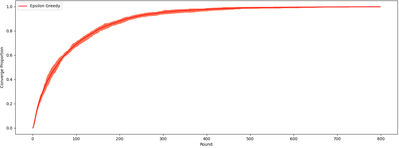
Figure 3: Error Bar of $\epsilon$-Greedy in Section 5.

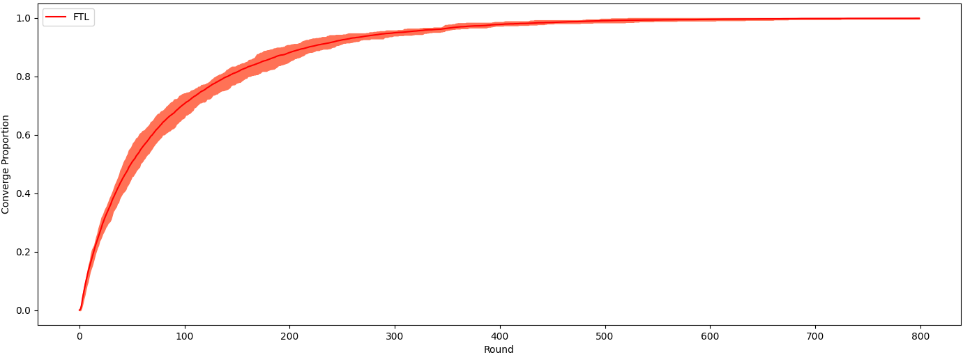
Figure 4: Error Bar of FTL in Section 5.

Figure 5: Error Bar of FPL2 in Section 5.

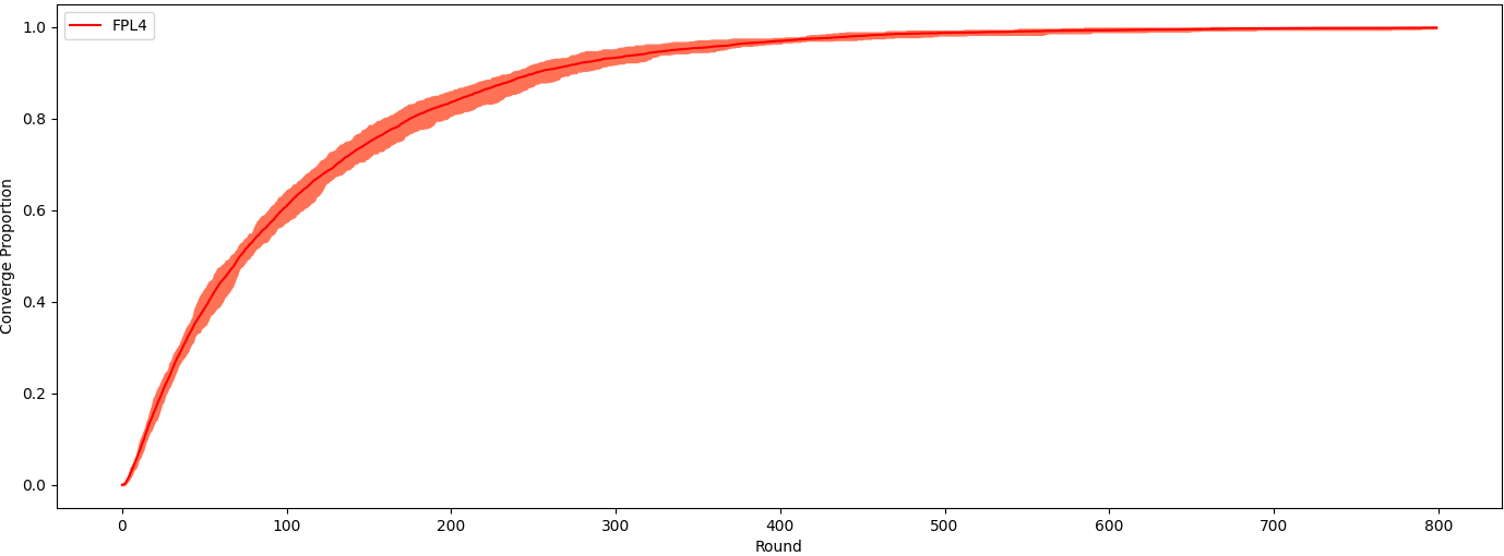
Figure 6: Error Bar of FPL4 in Section 5.

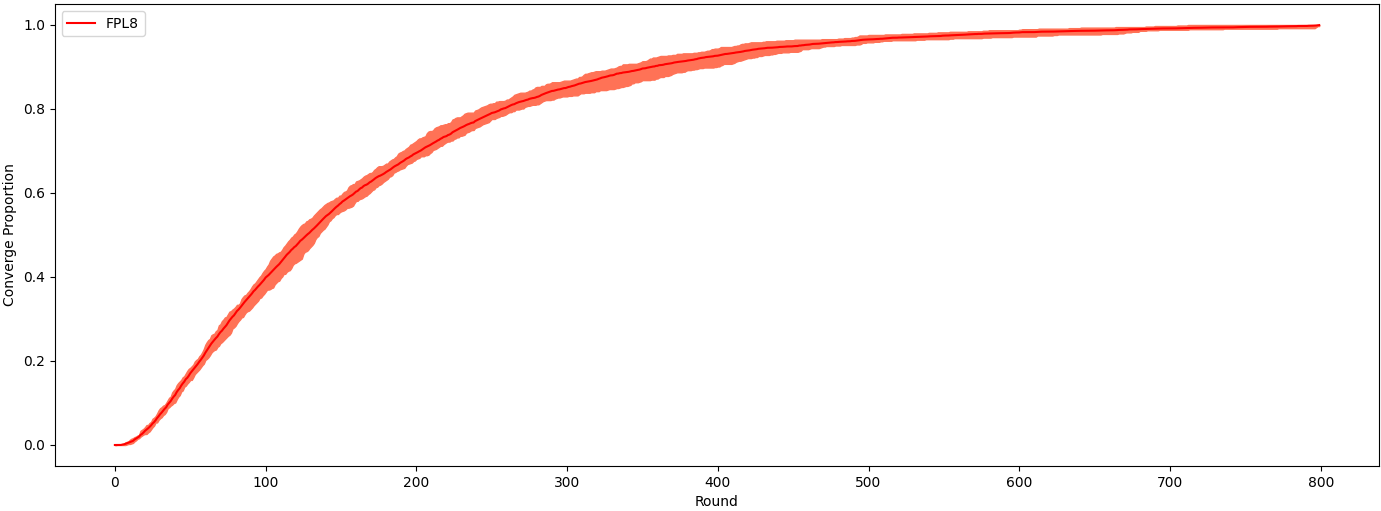
Figure 7: Error Bar of FPL8 in Section 5.

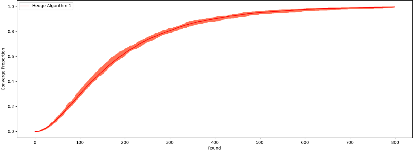
Figure 8: Error Bar of Hedge Algorithm 1 in Section 5.

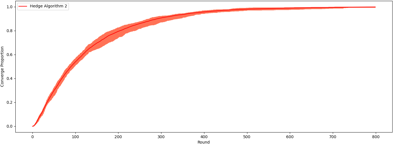
Figure 9: Error Bar of Hedge Algorithm 2 in Section 5.

References

• Alon and Spencer [2016] N. Alon and J. H. Spencer. The probabilistic method. John Wiley & Sons, 2016.
• Arora et al. [2012] S. Arora, E. Hazan, and S. Kale. The multiplicative weights update method: a meta-algorithm and applications. Theory of computing, 8(1):121–164, 2012.
• Braverman et al. [2017] M. Braverman, J. Mao, J. Schneider, and S. M. Weinberg. Selling to a no-regret buyer. CoRR, abs/1711.09176, 2017. URL http://arxiv.org/abs/1711.09176.
• Camara et al. [2020] M. K. Camara, J. D. Hartline, and A. Johnsen. Mechanisms for a no-regret agent: Beyond the common prior. In 2020 IEEE 61st Annual Symposium on Foundations of Computer Science (FOCS), pages 259–270. IEEE, 2020.
• Dasgupta and Ghosh [2013] A. Dasgupta and A. Ghosh. Crowdsourced judgement elicitation with endogenous proficiency. In Proceedings of the 22nd international conference on World Wide Web, pages 319–330, 2013.
• Deng et al. [2022] X. Deng, X. Hu, T. Lin, and W. Zheng. Nash convergence of mean-based learning algorithms in first price auctions. In Proceedings of the ACM Web Conference 2022, pages 141–150, 2022.
• Deng et al. [2019] Y. Deng, J. Schneider, and B. Sivan. Strategizing against no-regret learners. Advances in neural information processing systems, 32, 2019.
• Epstein [2012] R. A. Epstein. The theory of gambling and statistical logic. Academic Press, 2012.
• Faltings et al. [2014] B. Faltings, R. Jurca, P. Pu, and B. D. Tran. Incentives to counter bias in human computation. In Second AAAI conference on human computation and crowdsourcing, 2014.
• Feller [2008] W. Feller. An introduction to probability theory and its applications, vol 2. John Wiley & Sons, 2008.
• Freund and Schapire [1997] Y. Freund and R. E. Schapire. A decision-theoretic generalization of on-line learning and an application to boosting. Journal of computer and system sciences, 55(1):119–139, 1997.
• Hannan [1957] J. Hannan. Approximation to bayes risk in repeated play. Contributions to the Theory of Games, 3(2):97–139, 1957.
• Kajii and Morris [1997] A. Kajii and S. Morris. The robustness of equilibria to incomplete information. Econometrica: Journal of the Econometric Society, pages 1283–1309, 1997.
• Kalai and Vempala [2005] A. Kalai and S. Vempala. Efficient algorithms for online decision problems. Journal of Computer and System Sciences, 71(3):291–307, 2005.
• Kamble et al. [2015] V. Kamble, N. Shah, D. Marn, A. Parekh, and K. Ramachandran. Truth serums for massively crowdsourced evaluation tasks. arXiv preprint arXiv:1507.07045, page 96, 2015.
• Kong [2019] Y. Kong. Dominantly truthful multi-task peer prediction with a constant number of tasks. CoRR, abs/1911.00272, 2019. URL http://arxiv.org/abs/1911.00272.
• Kong and Schoenebeck [2016a] Y. Kong and G. Schoenebeck. Equilibrium selection in information elicitation without verification via information monotonicity. arXiv preprint arXiv:1603.07751, 2016a.
• Kong and Schoenebeck [2016b] Y. Kong and G. Schoenebeck. A framework for designing information elicitation mechanisms that reward truth-telling. CoRR, abs/1605.01021, 2016b. URL http://arxiv.org/abs/1605.01021.
• Liu and Chen [2018] Y. Liu and Y. Chen. Surrogate scoring rules and a dominant truth serum for information elicitation. arXiv preprint arXiv:1802.09158, 2018.
• Miller et al. [2005] N. Miller, P. Resnick, and R. Zeckhauser. Eliciting informative feedback: The peer-prediction method. Management Science, 51(9):1359–1373, 2005.
• Prelec [2004] D. Prelec. A bayesian truth serum for subjective data. science, 306(5695):462–466, 2004.
• Prelec et al. [2017] D. Prelec, H. S. Seung, and J. McCoy. A solution to the single-question crowd wisdom problem. Nature, 541(7638):532–535, 2017.
• Radanovic and Faltings [2014] G. Radanovic and B. Faltings. Incentives for truthful information elicitation of continuous signals. In Proceedings of the Twenty-Eighth AAAI Conference on Artificial Intelligence, pages 770–776, 2014.
• Schoenebeck and Yu [2020] G. Schoenebeck and F. Yu. Learning and strongly truthful multi-task peer prediction: A variational approach. CoRR, abs/2009.14730, 2020. URL https://arxiv.org/abs/2009.14730.
• Schoenebeck et al. [2021] G. Schoenebeck, F.-Y. Yu, and Y. Zhang. Information elicitation from rowdy crowds. In Proceedings of the Web Conference 2021, pages 3974–3986, 2021.
• Shnayder et al. [2016a] V. Shnayder, A. Agarwal, R. M. Frongillo, and D. C. Parkes. Informed truthfulness in multi-task peer prediction. CoRR, abs/1603.03151, 2016a. URL http://arxiv.org/abs/1603.03151.
• Shnayder et al. [2016b] V. Shnayder, R. Frongillo, and D. C. Parkes. Measuring performance of peer prediction mechanisms using replicator dynamics. In Proceedings of the Twenty-Fifth International Joint Conference on Artificial Intelligence, 2016b.
• Witkowski and Parkes [2012] J. Witkowski and D. C. Parkes. A robust bayesian truth serum for small populations. In Twenty-Sixth AAAI Conference on Artificial Intelligence, 2012.
• Zheng et al. [2021] S. Zheng, F. Yu, and Y. Chen. The limits of multi-task peer prediction. CoRR, abs/2106.03176, 2021. URL https://arxiv.org/abs/2106.03176.