Hadronic structure on the light-front V.
Diquarks, Nucleons and multiquark Fock components

Abstract

This work is a continuation in our series of papers, that addresses quark models of hadronic structure on the light front, motivated by the QCD vacuum structure and lattice results. In this paper we focus on the importance of diquark correlations, which we describe by a quasi-local four-fermion effective ’t Hooft interaction induced by instantons. The same interaction is also shown to generate extra quark-antiquark pair of the “sea". Its higher order iteration can be included via “pion-mediation": both taken together yield a quantitative description of the observed flavor asymmetry of antiquarks sea. Finally we discuss the final step needed to bridge the gap between hadronic spectroscopy and parton observables, by forward DGLAP evolution towards the chiral upper scale of $\sim 1\,{\rm GeV}^{2}$.

I Introduction

Since this paper is the fifth in our series Shuryak and Zahed (2021a, b, c, 2022), it does not need an extended Introduction, other than for issues not considered in the previous papers. So, we start directly by outlining its content.

The two introductory subsections I.1 and I.2, are devoted to diquark correlations in baryons and multiquark hadrons, respectively. Diquark “spectrosopy" has a rather long history which includes empirical facts, and dynamical calculations (NJL model, instantons, lattice). Furthermore, by identifying certain four-quark effective interactions, one naturally can proceed to the evaluation of their role not only in the $2\leftrightarrow 2$ channels, but also in the $1\rightarrow 3$ channel, and in the coupling of the 3q and 5q sectors in baryons.

The introductory subsection I.2 outlines our general strategy to “bridge" hadronic spectroscopy and partonic observables. The $1\rightarrow 3$ processes are the first step towards the creation of the “hadronic sea" of quarks and antiquarks, which complements perturbative DGLAP evolution, as it is clear from the flavor asymmetry of antiquarks.

We start our studies of diquark correlations from the nonrelativistic setting in section II.1, where we compare the effects of the perturbative Coulomb and instanton-induced ’t Hooft interactions using some simple variational approaches. Its main conclusion is that diquark correlations are strong, and that the ’t Hooft interaction is dominant. In section III, the diquark problem is treated on the light front, by a Hamiltonian similar to the meson one, using a quasilocal $qq$ interaction. In section IV we present a simplified analysis of baryons in the CM frame, using Coulomb and ^′t Hooft interactions only.

The next section deals with baryons on the light front, it starts with V.1 where we derive the LFWFs deformation by a heavy quark mass. Note that in our previous analysis in Shuryak and Zahed (2022), we only considered flavor symmetric baryons $qqq,sss,ccc,bbb$. Here instead, we consider heavy-light baryons such as $\Lambda_{Q}=Qud$ with a single diquark in V.2, before addressing the diquark pairing in the nucleon in section VI. We further elucidate the observable consequences of this pairing by calculating the formfactors for the isobar Delta and the Nucleon in section VII.

In section VIII.1 we show how to ^′ bridge the gap^′ between the spectroscopic analysis and the partonic observables, using the chiral processes discussed in section VIII. More specifically, in VIII.1 we motivate the selection of the scale where the chiral theory and perturbative DGLAP evolution match. In VIII.2 we detail the empirical information on the flavor asymmetry of the antiquark sea of the nucleon. We present two mechanisms for this effect, one using the first order in ’t Hooft Lagrangian  VIII.3, and the other a pion-mediated processe VIII.4, each of which is illustrated in Fig.1. The matching of the chiral and perturbative evolutions are discussed in section VIII.5.

The last section IX summarizes the main results of our series of papers. A number of more technical issues are discussed in the Appendices.

I.1 Diquark correlations

Diquark correlations of light quarks in nucleons and hadronic reactions, have been extensively discussed in the literature in the past decades, see e.g. Carroll et al. (1968); Jaffe and Wilczek (2003), and more recently in the review Barabanov et al. (2021). Here, we will not cover their phenomenological contributions to various hadronic reactions, but rather address some theoretical considerations about their dynamical origins based on semiclassical instantons. We will also cover recent lattice advances in diquark studies.

In two-color QCD with $N_{c}=2$, diquarks are baryons. In the chiral limit, QCD with two colors and flavors, admit Pauli-Gursey symmetry, an extended SU(4) symmetry that mixes massless baryons and mesons. In three-color QCD with $N_{c}=3$, diquarks play an important role in the light and heavy light baryons.

The simplest way to understand diquark correlations in hadrons, is in single-heavy baryons where the heavy spectator quark compensates for color, without altering the light diquark spin-flavor correlations. A good example are $Qud$ baryons, with $\Sigma_{Q}$ composed of a light quark with a flavor symmetric assignment $I=1,J^{P}=1^{+}$, and $\Lambda_{Q}$ composed of a light quark pair with a flavor asymmetric assignment $I=0,J^{P}=0^{+}$ state, the so called bad and good diquark states. Note that the latter has no spin, and thus no spin-dependent interaction with the heavy quark $Q$, while the former does. However, assuming that the standard spin-spin interactions are of the form $(\vec{\sigma}_{1}\vec{\sigma}_{2})$, this spin interaction can be eliminated as follows

$$M(1^{+}ud)-M(0^{+}ud)$$ (1)

$$\approx\big{(}(2M(\Sigma^{*}_{Q})+M(\Sigma_{Q})/3\big{)}-M(\Lambda_{Q})\approx 0.21\,{\rm GeV}$$

with the numerical value thus obtained from experimental masses of $cud,bud$ baryons yields the binding of two types of light quark diquarks. We note tha the mass difference between heavy-light baryon and meson iof $m(Qud)-m(Qu)\approx 329\,MeV$, is close to a constituent quark mass, but does not seem to include any extra contribution to the kinetic energy of the extra quark. Apparently, it is cancelled by some attraction.

With antisymmetric color and spin wave function, scalar diquarks must also be antisymmetric in flavor: so those can only be $ud,us,sd$ pairs. Those are called “good" diquarks in the literature, in contrast to the “bad" ones made of same flavor $dd,uu,...bb$ and, by Fermi statistics, with a symmetric spin $S=1$ wave functions.

The role of the light fermionic zero modes induced by instantons, at the origin of the ’t Hooft effective Lagrangian for chiral symmetry breaking, and their importance for pions and other aspects of chiral symmetry breaking are well known, for a review see e.g. Schäfer and Shuryak (1998). Diquark correlations induced by the ’t Hooft interaction were found in studies of the nucleons in instanton ensembles in Schäfer et al. (1994). In particular, the "good" diquark mass was found to be $m(0^{+})\approx 420\,MeV$, while the “bad" vector diquark mass was found to be $m(1^{+})\approx 940\,MeV$, with a difference as large as $500\,MeV$.

Although only a Fiertz transformation is needed from a meson to a diquark channel, this phenomenon has been originally considered only by few Betman and Laperashvili (1985); Praschifka et al. (1989); Thorsson and Zahed (1990), before the realization that diquarks would turn to Cooper pairs in dense quark matter, as pointed out in Rapp et al. (1998); Alford et al. (1998). (For subsequent review on “color superconductivity" see Schäfer and Shuryak (2001).)

Theoretically, it was important to note that in $SU(2)$ color theory, the scalar diquarks are massless partners of the Goldstone mesons  Rapp et al. (1998). By continuation to $SU(3)$ color, one then expects “good" scalar diquarks to be deeply bound as well. The ratio of the color factors, between the pseudoscalar meson (pions or $\eta^{\prime}$) channels, and the scalar diquark channel, is the same for the perturbative one-gluon exchange and the instanton-induced ’t Hooft vertex.

$$\frac{G_{qq}}{G_{\bar{q}q}}={1\over N_{c}-1}$$ (2)

Note that it is $1$ for $SU(2)$ color, supporting Pauli-Gursey symmetry between diquarks (baryons in this theory) and mesons. It is $1/2$ for the $SU(3)$ color case of interest, and zero in the $N_{c}\rightarrow\infty$ limit.

Calculation of (pseudoscalar and vector) meson and (scalar and vector) diquark DAs using Bethe-Salpeter equation with NJL kernels were originally carried in Thorsson and Zahed (1990), and more recently in Lu et al. (2021).

Lattice studies of light diquarks have also a long history, with the ealy analyses in Green et al. (2010) to recent studies in Francis et al. (2022). Diquarks are either studied inside dynamical baryons, or by tagging a Wilson line to a $qq$ pair as a heavy-light $Qqq$-type baryon. We already noted the mass difference between the vector and scalar $ud$ diquarks, with the lattice estimate putting it at $m(1^{+})-m(0^{+})\approx 200\,MeV$. The lattice studies show that in $Qud$ baryon, the light quarks are correlated together, but in a region of about $r_{0}\approx 0.6\,fm$ size, which is twice larger than suggested in earlier papers.

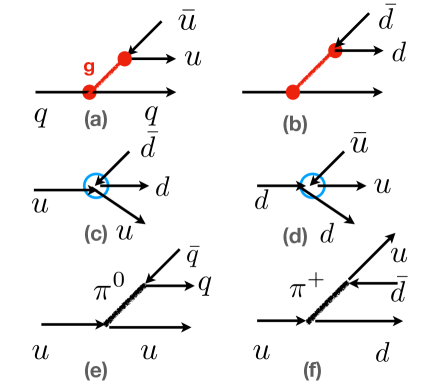
Figure 1: Upper raw (a,b): gluon-mediated quark pair production; Middle raw (c,d): instanton-induced ’t Hooft four-fermion interaction; Lower raw (e,f): pion-mediated quark pair production, or iterated ’t Hooft Lagrangian in $s$ and $t$ channels.

To complete our introduction to diquarks, we briefly note the issue of heavy diquarks, e.g. made of two charmed quarks $cc$. This issue reappeared after the recent discovery of the tetraquark $T_{cc\bar{u}\bar{d}}^{++}$ by the LHCb collaboration. If the only force is Coulomb, the $QQ$ coupling is half of that in $\bar{Q}Q$. Now, since for a $1/r$ potential the binding scales as the $square$ of the coupling, we readily get $B(QQ)={1\over 4}B(\bar{Q}Q)$. Yet we do know that charm quarks are not heavy enough to ignore the confining forces in charmonium, and so this relation is not expected to hold. The static potentials between heavy quarks were discussed in detail in our previous paper Shuryak and Zahed (2022).

Karliner and Rosner Karliner and Rosner (2014, 2017) conjectured a different relation

$$B(QQ)={1\over 2}B(\bar{Q}Q)$$ (3)

which turned out to be phenomenologically successful. (While it resembles what we called in our previous paper “Ansatz A" for the quark-quark static interaction, it is not the same, a half for $potentials$ is not half for $bindings$. For charmonium binding in their analysis $B(\bar{Q}Q)\approx-258\,MeV$, so $B(QQ)\approx-129\,MeV$, which led them to a predict a mass of $M(T_{cc\bar{u}\bar{d}}^{++})=3882\,MeV$ just $7\,MeV$ above the subsequent experimentally measured value.)

Currently we have not performed any calculations for tetraquarks. We had done some preliminary studies of heavy-heavy-light $QQq$ baryons with some model wave functions, and concluded that for two charm quarks $QQ=cc$ their separation into quasi-two-body (heavy diquark plus light “atmosphere") is not really justified. This is in qualitative agreement with the relatively small binding of a $cc$ diquark in the Karliner-Rosner conjecture. So, in this work, we will focus on the light-light “good diquarks", known to be more strongly bound.

I.2 Bridging the gap between hadronic spectroscopy and partonic physics

In this subsection we outline our plan for bridging this gap.

Our starting point is the well known traditional quark model used in hadronic spectroscopy. The main phenomenon included in this model is the lhenomenon of chiral symmetry breaking, with an effective mass for the “constituent quarks". For light quarks it is $m_{q}\sim 1/3\,GeV$. This mass is much smaller than the induced mass on gluons, so hadronic spectroscopy is traditionally described as bound states of these constituent quarks, with gluonic states or excitations described as “exotica". The traditional states are two-quark mesons and three-quark baryons, but of course there are also $tetraquarks$ $q^{3}\bar{q}$ and $pentaquarks$ $q^{4}\bar{q}$ states, recently discovered with heavy quark content.

The first ark of the bridge (described in detail in these series of works) is to transfer such quark models from the CM frame to the light front. For some simplest cases – like heavy quarkonia – it amounts to a transition from spherical to cylindrical coordinates, with subsequent transformation of longitudinal momenta into Bjorken-Feynman variable $x$. But in general, it is easier to start with light-front Hamiltonians $H_{LF}$ and perform its quantization. One of the benefit is that no nonrelativistic approximation is needed, therefore heavy and light quarks are treated in the same way.

The second ark of the bridge is built via chiral dynamics , which seeds the quark sea by producing extra quark-antiquark pair. In section VIII we discuss how it can be done, in the first order in ’t Hooft effective action as well as via intermediate pions.

We will then argue that as the third ark of the bridge one should use the well known DGLAP evolution of the PDFs (perhaps modified), down to the scale at which there are no gluons. There the $q\bar{q}$ sea should be reduced to only the part generated by chiral dynamics (step two). The antiquark flavor asymmetry $\bar{d}-\bar{u}$ is the tool allowing us to tell gluon and chiral contributions, as it cannot be generated by “flavor blind" gluons.

II Dynamical binding of diquarks

II.1 Nonrelativistic studies of the role of Coulomb and ’t Hooft attractions

In the previous papers of this series we have shown how two basic nonperturbative phenomena can be included in the light front formulation:
(i) chiral symmetry breaking represented by “constituent" quark masses,
(ii) confinement represented by classical relativistic string.
By adding the light-front form of the kinetic energy of the constituents, we derived our basic Hamiltonian, modulo Coulomb, spin-spin and and spin-orbit effects. The eigenstates of this Hamiltonian, were evaluated using different methods.

Now we are going to focus on the “residual" interactions, namely:
(iii) perturbative Coulomb interactions,
(iv) various forms of quasi-local operators descending from ’t Hooft effective Lagrangian, or, more generally, from instanton-induced zero modes for light fermions
(v) effects due to the gauge fields of the instantons via nonlocal correlators of Wilson lines.

The traditional starting point is the nonrelativistic Schroedinger equation in the CM frame. As a compromise needed for the use of both a nonrelativistic approximation and the ’t Hooft Lagrangian, we focus initially on the $strange$ quark channel, with a constituent mass mass $m_{s}=0.55\,GeV$. As for any compromise, it is not really accurate, yet it will provide a preliminary information on the relative role of all the interactions listed above.

Since the ’t Hooft interaction must be flavor-asymmetric, we have to invent $another$ quark flavor $s^{\prime}$ with the same mass. (This idea is not ours, it originated in lattice studies where it is used to eliminate two-loop diagrams. The pseudoscalar $\bar{s}s^{\prime}$ meson even has an established name $\eta_{s}$.)

We start with a $variational$ approach, using simplified trial wave functions of two types

$$\psi_{A}\sim e^{-\alpha r^{2}},\,\,\psi_{B}\sim e^{-\beta r^{3/2}}$$ (4)

to be referred to as trial functions A and B. The former (Gaussian) form leads to simple analytical expressions for the mean kinetic energy, $\langle 1/r\rangle,\langle r\rangle,\langle\delta^{3}(\vec{r})\rangle$. However, the trial function B with the power of the distance in the exponent following from its semiclassical asymptotics, turns out to be closer in shape to the numerical solution. Some details about these variational functions can be found in Appendix A.

Let us summarize the qualitative lessons we got from these variational studies. First, we demonstrate that the contributions of both attractive forces – the Coulomb and the ’t Hooft ones – are comparable for the strange quark mass. The light diquark binding and the r.m.s. size suggested by phenomenology and observed on the lattice, can be explained with the conventional values for the Coulomb and ’t Hooft couplings.

Second, we find the following distinction between these interactions: their contribution to the binding can change significantly if these values are changed. For example, if the diquark size is reduced by a factor two, $\langle 1/r\rangle$ increases by a factor of 2, while $\langle\delta^{3}(\vec{r})\rangle$ increases by a factor $2^{3}=8$ and becomes dominant. So a reported balance between perturbative and nonperturbative contributions to the binding, is in fact only valid for a strange quark mass, and is very sensitive to the actual quark masses.

Of course, in the current setting, there is no problem to solve the Schroedinger equation numerically. For convenience, we represent the ’t Hooft quasi-local term $-G_{qq}\delta^{3}(\vec{r})$ by a smeared delta function. In Fig.14 the resulting ground state wave functions are compared, for four values of the coupling $G_{dq}=0,10,20,30\,GeV^{-2}$. As expected, an increase in the negative potential near the origin, leads to a large wave function at small $r$.

In Table 1 we give the corresponding r.m.s. sizes and binding energies for the lowest four states. One can see that in order to get a binding of $\sim-0.2\,GeV$ and a size of $\sim 0.6\,fm$, indicated by lattice studies, the coupling needs to be $G_{qq}\sim 20\,GeV^{-2}$. Recall that by Fiertzing the ’t Hooft operator from the $\bar{q}q$ to $qq$ channel, there is an additional factor of $1/(N_{c}-1)=1/2$. So this value corresponds to the coupling in mesons of $\sim 40\,GeV^{-2}$. Finally, we note that both the ’t Hooft and Coulomb bindings are only strong for the ground state, and their effect is strongly decreasing with $n$, as is listed in this Table.

Table 1: Root-mean-square sizes (fm) and additional binding energies (GeV) for the lowest four states of $ss^{\prime}$ diquarks, for four values of the $qq$ ’t Hooft coupling

$G_{qq}\,GeV^{-2}$	$R_{r.m.s}\,fm$	$E_{0}-E_{0}(G_{qq}=0)$	$E_{1}-E_{1}(G_{qq}=0)$	$E_{2}-E_{2}(G_{qq}=0)$	$E_{3}-E_{3}(G_{qq}=0)$
0	0.67	-	-	-	-
10	0.62	-0.082	-0.044	-0.032	-0.026
20	0.56	-0.187	-0.089	-0.063	-0.051
30	0.50	-0.318	-0.132	-0.093	-0.074

III Diquarks on the light front

In order $not$ to use the nonrelativistic approach for the light quark systems, in the previous papers of this series we have advocated the use of the light front Hamiltonians. The confining forces were reduced by the ^′einbein trick^′. The resulting Hamiltonian $H_{LF}=H_{0}+V$, consits of $H_{0}$ which is the sum of a harmonic oscillator in transverse momenta plus a Laplacian for longitudinal momenta, and of $V$ wich includes transverse momenta in the numerator and longitudinal ones in the denominator. One strategy of solving this Hamiltonian is, following our predecessors Jia and Vary (2019), is to express $V$ as a matrix in the eigenbasis of $H_{0}$, with its subsequent diagonalization. In paper Shuryak and Zahed (2021b) we have checked the wave functions obtained by this method with direct 3d numerical solutions, with very good agreement between the two.

Here we propose another method of solution for $H_{LF}$, relying on the approximate factorization of the transverse and longitudinal degrees of freedom. Treating the mean square of the transverse momentum as a parameter, we focus on the longitudinal wave equation following from the relevant part of $H_{LF}$, which is proportional to

$$- {d^{2}\psi(x)\over dx^{2}}+A\bigg{(}{M_{1}^{2}+\langle\vec{p}_{\perp}^{2}\rangle\over x}+{M_{2}^{2}+\langle\vec{p}_{\perp}^{2}\rangle\over 1-x}$$ (5)

$$- 2(M_{1}^{2}+M_{2}^{2}+2\langle\vec{p}_{\perp}^{2}\rangle)\bigg{)}\psi(x)$$

The second derivative comes from the confining term (with parameter $a$ inherited from the “einbine trick") following the substitution of the longitudinal coordinate as $r_{l}\rightarrow id/dx$. The “potential" is written for two distinct masses, to keep it general. The mean squared transverse momentum is used as an external parameter, together with the quark masses. The last term with the minus sign in the “potential" is artificially subtracted here, and added in the remaining part of the $M_{2}$ for convenience (it is independent of the longitudinal momentum fraction $x$.)

The constant $A=a/\sigma_{T}$ in front of the potential contains the string tension $\sigma_{T}=(0.4\,GeV)^{2}$, and a parameter $a$ from the “einbine trick" we have used (which is fixed by minimizing the total mass squared).

Figure 2: Effective potentials in the longitudinal Hamiltonian (5), for a $qq$ pair (black curve), for a $sq$ pair (blue dashed curve), for a $cq$ pair (red dashed curve) and for a $c-(ud)$ charm-light diquark case (brown dash-dotted curve).

In Fig.2 we show the shape of the corresponding effective potentials for four cases:
(i) a pair of light constituent quarks $qq$ with masses $M_{1}=M_{2}=0.28\,GeV$ with comparable mean squared transverse momentum $\langle\vec{p}_{\perp}^{2}\rangle=(0.3\,GeV)^{2}$
(ii) a strange-light pair (e.g. $K^{*}$ vector mesons)
(iii) a charm-light pair (e.g. $D^{*}$ vector mesons)
(iv) a charm-$ud$ diquark, an approximation to $cud$ or $\Lambda_{c}$ baryon. We use here the diquark mass $m_{ud}=0.5\,GeV$
As one can see, the potential is small and symmetric in the $qq$ case (i), except near the edges of the physical domain, $x=0,$ and $x=1$. Yet the potential becomes very asymmetric if the two masses are different.

We solved the longitudinal wave equation following from (5) for two light quarks (case (i)), and compared the solution (shown by a black line in Fig.3)e to two functions which are often used as simple approximations to these wave functions.

(Note that in the approximation of constant $p_{\perp}$ distribution, these functions directly coincide with the Distribution Amplitudes (DAs). Therefore we have used here a normalization traditionally used for DAs, by putting to unity the integral of its $first$ power rather than the integral of the square, which is more appropriate for the wave functions.)

Figure 3: Longitudinal wave function for a diquark made of identical light quarks (black line, upper curve at the central point $x=1/2$). For comparison we also show the lowest harmonic function $sin(\pi x)$ by a blue line, and the “asymptotic" wave function $x(1-x)$ by the red line.

It is then straightforward to solve the equation (5) for the remaining three cases. All these ground state wave functions are shown in Fig. 4, in the upper plot as numerical solution $\psi(x)$, and in the lower plot as its Fourier transform $\psi(Pr_{l})$. The asymmetric potentials lead to rather asymmetric wave functions, shifting toward larger $x$ of the first (heavier) particle. This makes sense, since the pair binding requires that the constituents move with the same relative velocity, which translates to a larger momentum fraction carried by the heavier quark.

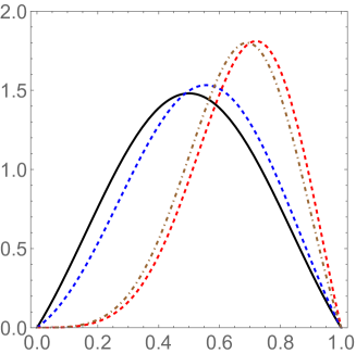
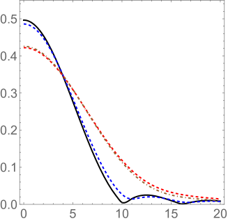
Figure 4: The wave functions as a function of the momentum fraction $\psi(x)$ (upper plot) and their Fourier Transform into coordinate space $\psi(P*r_{l})$ (lower plot). The marking of the four curves in both plots are the same, and identical to those used fin Fig.2: for the $qq$ pair it is the black curve, for the $sq$ pair it is the blue dashed curve, for the $cq$ pair it is the red dashed curve, and for the $c-(ud)$ charm-light diquark case it is the brown dash-dotted curve.

For completeness, let us give the (dimensionless) values of the ground state eigenvalues : those are

$$12.78,14.23,-8.10,-0.23$$

for these four cases respectively.

The wave functions dependence on the transverse momenta is (near) Gaussian, and can be readily Fourier transformed. So, with the longitudinal wave functions Fourier transformed into the $coordinate$ representation, we can calculate the matrix elements of any coordinate-dependent operators, such as the perturbative Coulomb. However in this paper we would not do so. We will only only consider the quasilocal ’t Hooft operator, which can be done without any Fourier transform.

IV Simplified baryons with Coulomb and ’t Hooft interactions in the CM frame

In this section we proceed from two quarks in a diquark to three quarks in a baryon, including the “residual" interactions beyond confinement. As for diquarks, we start with a preliminary study of three nonrelativistic quarks with equal masses in the CM frame, and proceed in three steps: (i) a “basic" 3-body problem, with only kinetic and confining energies; (ii) adding Coulomb interaction; (iii) adding quasi-local ’t Hooft interaction.

To discuss the three-body Hamiltonians and wave functions, we first rrecall how the three coordinate vectors $\vec{x}_{i}$ are redefined in terms of two Jacobi vectors $\vec{\rho}_{i},\vec{\lambda}_{i}$ (see (V.1) for their longitudinal analog), with the kinetic energy

$$H_{kin}=-\frac{1}{2M}\frac{\partial^{2}}{\partial\vec{X}^{2}}-\frac{1}{2m}\bigg{(}\frac{\partial^{2}}{\partial\vec{\rho}^{2}}+\frac{\partial^{2}}{\partial\vec{\lambda}^{2}}\bigg{)}$$ (6)

The first term, represents the center of mass motion, and is factored out. The remaining dynamics is performed in the remaining six dimensions.

We start with the basic problem, with only the kinetic and confining energy. In this case the problem is spherically symmetric in 6d and one can define the hyperspherical radius

$$R^{2}=\vec{\rho}_{ij}^{2}+\vec{\lambda}_{ij}^{2}$$ (7)

(with any pair combination $[ij]$, over which no summation will be assumed). (6) is the 6-d Laplacian

$$H_{kin}=-\frac{1}{2}\bigg{(}{\partial^{2}\over\partial R^{2}}+{5\over R}{\partial\over\partial R}\ \bigg{)}+{L^{2}\over 2R^{2}}$$ (8)

where $L$ includes derivatives over the angles. The ground state wave function may be assumed to depend only on the hyperradius $R$.

However, since we will consider a case in which one quark pair 1-2 will have a ’t Hooft attraction, there is no such symmetry, and we expect a different dependence on $\rho=|\vec{\rho}|$ and $\lambda=|\vec{\lambda}|$. We will use the following two-parameter Gaussian Ansatz

$$\psi(\rho,\lambda)=(2\alpha\beta/\pi)^{3/2}\,e^{-\alpha^{2}\rho^{2}-\beta^{2}\lambda^{2}}$$ (9)

The kinetic energy is then

$$E_{kin}={3\over 2m}(\alpha^{2}+\beta^{2})$$ (10)

The confining energy is then

$$E_{conf}=\sigma_{T}\langle\sqrt{2}\rho+\sqrt{3/2}\lambda\rangle=\sigma_{T}{\sqrt{3}\alpha+2\beta\over\sqrt{\pi}\alpha\beta}$$ (11)

where the first term includes the distance between the quarks 1 and 2, and the second term the distance from quark 3 to the CM of the first pair. Here and below, the angular brackets stand for the averaging over the wave function.

Using our standard set of parameters, with the strange quark mass $m=0.55\,GeV$, and the string tension $\sigma_{T}=(0.4\,GeV)^{2}$, we minimize these expressions and get variational wave function for the “basic" baryons, with only the confining force written in this approximation. The minimum of the energy is at $\alpha_{min}=0.32,\,\beta_{min}=0.31\,\,GeV^{-1}$, and the minimal values of the kinetic and confining energies are $E_{kin}\approx 0.38\,,E_{conf}\approx 1.07\,GeV$. (The slight asymmetry is caused by the asymmetric geometry of the confining string.)

Now we include the “residual" interactions, and minimize the total energy. The Coulomb interaction for the pair 12 includes the distance between these two quarks $r_{12}=\sqrt{2}\rho$, with

$$E_{Coulomb}=-{2\alpha_{s}\over 3}\bigg{<}{1\over r_{12}}\bigg{>}=-{2\alpha_{s}\over 3}{2\alpha\over\sqrt{\pi}}$$ (12)

The ’t Hooft Lagrangian induces a quasi-local 4-fermion operator, which we regulate using a Gaussian form with an fixed instanton size $\rho_{0}$,

$$E_{{}^{\prime}tHooft} = -G_{qq}\bigg{<}\frac{e^{-\rho^{2}/\rho_{0}^{2}}}{\pi^{3/2}\rho_{0}^{3}}\bigg{>}$$ (13)

$$= -G_{qq}\alpha^{3}\bigg{(}{2\over\pi+2\pi\alpha^{2}\rho_{0}^{2}}\bigg{)}^{3/2}$$

Using our standard set of parameters, the strange quark mass $m=0.55\,GeV$, the string tension $\sigma_{T}=(0.4\,GeV)^{2}$, the Coulomb coupling from charmonium fit $4\alpha_{s}/3\approx 0.7$, the instanton size $\rho_{0}\approx 0.3\,fm\approx 1/(0.6\,GeV)$ and the quark-quark coupling $G_{qq}=20\,GeV^{-2}$, we minimize the total energy, the sum of the terms mentioned above, over the parameters of the Ansatz. With the Coulomb and ’t Hooft terms acting only between particles 12, we found that the minimum is at

$$\alpha_{min}=0.430\,GeV^{-1},\,\,\,\beta_{min}=0.306\,GeV^{-1},$$ (14)

Note that parameter alpha has changed significantly as compared to the “basic" model above.

Using it, one finds the relative contributions of different terms in the Hamiltonian to be in this case (in GeV)

$$E_{kin} \approx 0.76,\,\,E_{conf}\approx 0.93,$$ (15)

$$E_{Coulomb} \approx -0.17,\,\,E_{tHooft}\approx-0.28$$

The main lesson from this variational estimate, is that again, we see that the instanton-induced ’t Hooft effect is somewhat larger than the Coulomb interaction, and that together they can generate significant diquark binding comparable to the quark constituent mass $\sim 0.35\,GeV$.

We conclude this section with the following comments:
(i) The main lesson from this variational calculation is that the asymmetry induced by the “residual" Coulomb and ’t Hooft interactions is quite substantial, and therefore their perturbative account is $not$ justified.
(ii) The Coulomb and ’t Hooft attractions are so far included only for $one$ pair of quarks 1-2, out of three. If those would be multiplied by three, the attraction can basically cancel the kinetic and confinement energy, leaving the total mass close to its naive nonrelativistic value $3m$.
(iii) In our older paper Shuryak and Zahed (2004) we developed a schematic model with certain “quasi-supersymmetry" between $masses$ of constituent quarks and light “good diquarks". (Not between the number of states, as needed for true supersymmetry.) In particular, it put certain mesons and baryons into some (approximate) multiplets. A similar meson-baryon symmetry has been developed in Brodsky et al. (2015) based on a hybrid holographic approach. Naively the same multiplets would include tetraquarks, as diquark-diquark states: yet those were not observed. It implies that diquark-diquark interaction is strongly repulsive, violating this “quasi-supersymmetry".

V Heavy-light baryons with diquarks

V.1 Asymmetry induced in the longitudinal LFWFs by a heavy quark mass

In our previous paper Shuryak and Zahed (2022) we have studied flavor-symmetric baryons, $qqq,sss,ccc,bbb$. Such choice was motivated by both the additional kinematical symmetry in each case, as well as the absence of an instanton-induced flavor-antisymmetric ’t Hooft interaction.

The 3-body kinematics was discussed there in detail, and will not be repeated here. For completeness, we briefly recall our notations. We use the momentum representation and 6 Jacobi coordinates $\vec{p}_{\lambda},\vec{p}_{\rho}$. Their longitudinal momenta, normalized to total hadron momentum called “momentum fractions" $x_{i},i=1,2,3$, are expressed in two coordinates $\rho,\lambda$ as follows

$$x_{1} = 1/6(2+\sqrt{6}\lambda+3\sqrt{2}\rho);$$

$$x_{2} = 1/6(2+\sqrt{6}\lambda-3\sqrt{2}\rho)$$ (16)

$$x_{3} = 1/3(1-\sqrt{6}\lambda)$$

The physical domain of the $\rho,\lambda$ variables is an equilateral triangle, with corners corresponding to one of the momentum fractions reaching one, and the others zero.

The light front Hamiltonian considered in Shuryak and Zahed (2022) included the kinetic energy of quarks and confining term only. The latter term, with certain tricks, is made proportional to the 6-d quadratic form in coordinates. After those are changed to derivatives over momenta, it is amenable to transverse and longitudinal Laplacians. (This is so for both the $Y$ confining model, with three strings and a color junction, as well as for the “A Ansatz" with slightly different numerical coefficients.) Here we will focus on the ongitudinal momenta, so our main differential operator takes the form $\partial^{2}/\partial\rho^{2}+\partial^{2}/\partial\lambda^{2}$, defined on the equilateral triangle with corners at

$$(\rho,\lambda)=(0,-\sqrt{2/3}),(1/\sqrt{2},1/\sqrt{6}),(-1/\sqrt{2},1/\sqrt{6})$$

In Shuryak and Zahed (2022), its eigenfunctions were found analytically and numerically.

The kinetic part of Hamiltonian

$$H_{kin}=\sum_{i}{\vec{p}_{i\perp}^{2}+m_{i}^{2}\over x_{i}}$$ (17)

depends nontrivially on the longitudinal momentum fractions. It is convenient to subtract and add its value at the center point $x_{1}=x_{2}=x_{3}=1/3$ and call it a “potential" $V$ plus a term depending only quadratically on $\vec{p}_{\perp}$. The latter was used for the “transverse oscillator" part, defining the basis set of functions. The potential $V$ was included either in the form of a matrix in that basis, or found numerically from solving the Schroedinger-like equation.

The confining (Laplacian) part of the Hamiltonian does not depend on masses, but the potential $V$ does. If masses of the three quarks are the same (the case discussed in Shuryak and Zahed (2022)) it has a discrete symmetry corresponding to maps of the triangle into itself (rotations by the angle $\pm 2\pi/3$). This symmetry is shared by a Laplacian and thus the resulting wave functions. In this section we make the first step towards $unequal$ quark masses, where this symmetry is absent.

We are aiming first at heavy-light baryons of the type $qqQ$ (with light diquarks either flavor symmetric or antisymmetric), and introduce two dimensionless parameters

$$A_{Q}={\langle p_{Q\perp}^{2}\rangle+m_{Q}^{2}\over\sigma_{T}},\,\,\,A_{q}={\langle p_{q\perp}^{2}\rangle+m_{q}^{2}\over\sigma_{T}}$$ (18)

The denominators contain the string tension, while in the numerators we substituted the squared transverse momenta by their average. In this approximation the longitudinal degrees of freedom split from the transverse ones, with the effective dimensionless potential

$$\tilde{V}(\lambda,\rho)=A_{q}(1/x_{1}+1/x_{2}-6)+A_{Q}(1/x_{3}-3)$$ (19)

While it is still defined on the equilateral triangle, it no longer has the triple $2\pi/3$ symmetry. Specifically, we note that these parameters have very different magnitude for light and e.g. charmed quarks

$$(\langle p_{q\perp}^{2}\rangle+m_{q}^{2})/\sigma_{T}\approx 1.5,\,\,\,(\langle p_{c\perp}^{2}\rangle+m_{c}^{2})/\sigma_{T}\approx 15$$

For $b$ quarks the ratio is another order of magnitude larger. So the triple symmetry is very strongly broken by the leading term with a large heavy quark mass. The effect is so strong, even for charm quark, that one can only keep the $m_{c}^{2}(1/x_{3}-3)$ term in the kinetic energy.

We evaluated the matrix elements of the potential in the laplacian basis, and got the wave function of the $\Sigma_{Q}=Q(ud)_{1+}$ baryon. The ground wave functions represented as a combination of (12) basis states

$$\Psi_{\Sigma_{Q}(1)}=\sum_{n}C_{n}\psi_{n}(\rho,\lambda)$$ (20)

with the coefficients equal to

$$C_{n}^{\Sigma}=(0.520,0.025,0.736,-0.331,-0.167,-0.189,$$

$$-0.105,-0.009,-0.024,0.012,-0.014,-0.008)$$

Note that several of coefficients are comparable, and the first coefficient is not even the largest. It happens because the charm quark mass term creates such a large perturbation, that the lowest $\Sigma_{Q}(1)$ state is not even close to the lowest state of the Laplacian.

V.2 Diquark pairing in $\Lambda_{Q}$ baryons

Now we make the second step, to $\Lambda_{Q}=Q(ud)_{0^{+}}$ baryons with a flavor-asymmetric $ud$ diquark. In addition to what was discussed in the preceding section, now there is also the ’t Hooft determinantal interaction between the $ud$ quarks. The symmetry $1\leftrightarrow 2$ (or $\rho\leftrightarrow-\rho$) of the Hamiltonian and the LFWFs remains.

We now make use of a simplified and fully $local$ ^′t Hooft interaction

$$H_{ud}=-G_{ud}\delta(\vec{r}_{u}-\vec{r}_{d})$$ (21)

The matrix element of the $spatial$ delta functions is discussed in Appendix B, see (B). Using it in our set of basis functions, we performed those integrals and obtained the Hamiltonian in a form of a 12$\times$12 matrix. Multiplying it by the coupling $G$, adding it to Hamiltonian detailed in the previous sections and getting the eigensystem, we generated 12 states of the $\Lambda_{c}$ baryons. We have tuned the coupling so that the ground states have binding difference between “good" and "bad" diquark fixed by phenomenology (1).

After this is achieved, we can compare the obtained $\Sigma_{c}$ and $\Lambda_{c}$ light front wave functions. One way to do it is to give the coefficients of the decomposition in the Laplacian basis functions as we did above for $\Sigma_{c}$ . Those are

$$C_{n}^{\Lambda}=(0.625,0.025,0.725,-0.249,-0.079,-0.089,$$

$$-0.052,-0.004,0.040,-0.020,-0.0272,0.004)$$

see Fig.5 . We can see from the upper plot, differences at larger $\rho$ (lowest curves) that are as big as a factor of 2. However, a better representation of the shape $difference$ is given by the lowest plot

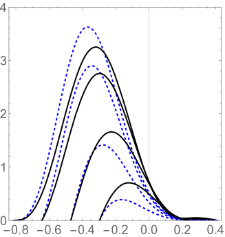
Figure 5: Upper plot: the longitudinal wave functions $\Psi_{\Sigma}(\rho,\lambda)$ of $\Sigma_{c}$ (blue dashed) and $\Psi_{\Lambda}(\rho,\lambda)$ of $\Lambda_{c}$ (black solid), as a function of $\lambda$. The four pairs of curves are for $\rho=0.0,0.1,0.2,0.3$, top to bottom. The lower 3D plot shows their $difference$, $\Psi_{\Lambda}(\rho,\lambda)-\Psi_{\Sigma}(\rho,\lambda)$ .

V.3 Instanton-induced effects in heavy-light hadrons

In the firts paper of this series Shuryak and Zahed (2021a), we have addressed the instanton effects on Wilson lines (heavy quark potentials). The novel point was the proposal of a “dense instanton liquid" that also includes instanton-antiinstanton molecules. In the second paper of the series Shuryak and Zahed (2021b) the instanton-induced t’ Hooft interaction was used for light quarks, in the context of the pion LFWF. Since this interaction follows solely from the near-zero fermionic modes, it is natural to limit its discussion to the ^′dilute instanton liquid^′ as we did, with the hope of avoiding any confusion.

In this section we review some applications to heavy-light hadrons. The pioneering study in the original instanton vacuum was carried by Chernyshev, Nowak and Zahed Chernyshev et al. (1995), on which this section is based. We will provide some further discussion, insuring connections to later papers and the remainder of our series.

qQ interaction: The main point is that the instanton field strength (acting on a static quark $Q$), and its zero mode (acting on a light quark $q$) are correlated. The appropriate setting is again the “dilute instanton liquid".

If the instanton size is small, it can be written as a quasilocal operator, to be included in a Lagrangian. The interaction between a single light quark $q$ and a single static heavy quark $Q$ is

$${\cal L}_{qQ}= -G_{Qq}\left(\overline{{\bf Q}}\frac{1+\gamma^{0}}{2}{\bf Q}\,\,\overline{{\bf q}}{\bf q}+\frac{1}{4}\overline{{\bf Q}}\frac{1+\gamma^{0}}{2}\lambda^{a}{\bf Q}\,\,\overline{{\bf q}}\lambda^{a}{\bf q}\right)$$

The light quark effective vertex is based on the representation of the propagator as

$$S_{ZM}(x,y)={\psi_{0}(x)\psi_{0}(y)\over m*}$$ (23)

with some effective “determinantal mass" characterizing the instanton ensemble. In the original ILM paper Shuryak (1982) this mass was directly related with the quark condensate

$$m^{*}=\frac{2}{3}\pi^{2}\rho^{2}|\langle\bar{q}q\rangle|\approx 170\,{\rm MeV}$$

(the number is for the empirical condensate value). Further development followed two directions: the gap equations in the mean field approximation (see references in Pobylitsa (1989)) and numerical simulations of the instanton ensemble. The former expressions were used in Chernyshev et al. (1995) with

$$m^{*}=\sqrt{\frac{n}{2N_{c}}}\Sigma_{0}$$

and the RILM instanton density $n=1\,{\rm fm}^{-4}$. (Note that in Chernyshev et al. (1995) the factor of $1/2N_{c}$, following from the averaging over the color moduli, was included in the definition of $n$). The explicit form of $\Sigma_{0}$ is quoted in Appendix E, with $\Sigma_{0}\approx 240\,MeV$. The typical coupling in (LABEL:qQ) in the RILM is

$$G_{Qq}=\bigg{(}\frac{\Delta M_{Q}\Delta M_{q}}{n}\bigg{)}$$ (24)

with the heavy quark mass shift

$$\Delta M_{Q}=-\frac{4\pi^{2}}{3\rho}\,\frac{\pi^{2}\rho^{4}n}{N_{c}}\,\bigg{(}J_{0}(\pi)+\frac{1}{\pi}J_{1}(\pi)\bigg{)}\sim 70{\rm MeV}$$

and the light quark mass shift $\Delta M_{q}$ given in Appendix E. We recognize in (V.3) the packing fraction $\kappa=\frac{1}{2}\pi^{2}\rho^{4}n$ in the RILM, also used in our earlier papers.

Note that (LABEL:qQ) is dominated by the color-matrix (Coulomb-like) second term and has a proper heavy quark spin symmetry. The spin-dependent correction is subleading in $\Delta M_{Q}^{spin}\sim 1/m_{Q}$

$${\cal L}_{qQ}^{spin}=\frac{\Delta M_{q}\;\Delta M_{Q}^{spin}}{n}\;\frac{1}{4}\;\overline{\bf Q}\frac{1+\gamma^{0}}{2}\lambda^{a}\sigma^{\mu\nu}{\bf Q}\,\,\overline{\bf q}\lambda^{a}\sigma^{\mu\nu}{\bf q}$$

For the charm quark

$$\Delta M_{Q}^{spin}=\frac{8\pi}{m_{Q}\rho^{2}}\frac{\rho^{4}n}{N_{c}}\int dx\,\frac{x^{2}{\rm sin}^{2}f(x)}{(1+x^{2})^{2}}\sim 3\,{\rm MeV}$$

with the profile $f(x)=\pi x/(1+x^{2})^{\frac{1}{2}}$.

qq interaction: The instanton-induced ’t Hooft Lagrangian has the form of a determinant in flavor indices of certain $\bar{q}q$ operators, so the total numbers of quark legs is $2N_{f}$. Elsewhere in our works we assumed that either there are only $u,d$ flavors, $N_{f}=2$ and the Lagrangian is of the usual four-fermion form, or that $N_{f}=3$ and the number of legs is 6, with the strange quarks contracted in the vacuum $\langle\bar{s}s\rangle$. However. we may ask if there are situations in the baryon sector whereby the full six-fermion operator may contribute. The operator, as any Lagrangian should be, is flavor $SU(3)$ singlet: therefore if used as a “baryonic current" operator aimed to $excite$ the vacuum into the $uds$ baryon, such baryon must be $SU(3)$ singlet as well. This condition is not fulfilled for the usual $\Lambda,\Sigma$ baryons which are members of the $SU(3)$ octet. There are known excited $\Lambda^{*},\Sigma^{*}$ $SU(3)$ singlets, but those have nonzero orbital momentum which the Lagrangian would not excite. Yet we think of averaging a 6-quark ’t Hooft Lagranian over $\Lambda,\Sigma$ baryons, it does generate a “superlocal" interaction (all three quarks at the same point, similar to Skyrme force in nuclear physics). We do not pursue this issue quantitatively and return to the 4-quark determinant.

In the rest frame and using nonrelativistic spinors, we have

$$H^{\eta^{\prime}}_{qq}\approx-\bigg{(}\frac{\Delta M^{2}_{q}}{n}\bigg{)}\frac{1}{2}(1-\tau_{1}\cdot\tau_{2})\delta(\vec{r}_{12})$$ (28)

with $\vec{r}_{12}=\vec{r}_{1}-\vec{r}_{2}$, in leading order in $1/m_{Q}$. The sign corresponds to the repulsive $\eta^{\prime}$ channel, which is seen to flip in the pion channel by dropping 1. On the light front, the reduction of the $\bar{q}q$ interaction in momentum space, is detailed in Appendix G. For a meson with a quark-antiquark pair and with zero transverse momentum in and out ($P_{T}=P_{T}^{\prime}=0$), the 2-particle interaction potential in momentum space is

$${\rm det}\overline{\bf q}_{L}{\bf q}_{R}\rightarrow(1-\tau_{1}\cdot\tau_{2})\bigg{(}m_{Q1}{\bf 1}_{1}+\frac{1}{2}\sigma_{1}^{-}q_{R}\bigg{)}\bigg{(}-m_{Q2}{\bf 1}_{2}+\frac{1}{2}\sigma_{2}^{+}q_{R}\bigg{)}$$

$${\rm det}\overline{\bf q}_{R}{\bf q}_{L}\rightarrow(1-\tau_{1}\cdot\tau_{2})\bigg{(}m_{Q1}{\bf 1}_{1}+\frac{1}{2}\sigma_{1}^{+}q_{L}\bigg{)}\bigg{(}-m_{Q2}{\bf 1}_{2}+\frac{1}{2}\sigma_{2}^{-}q_{L}\bigg{)}$$ (29)

with the transverse coordinates $q_{R,L}=q_{1}\pm iq_{2}$, and $\sigma^{\pm}=\sigma_{1}\pm i\sigma_{2}$. The contribution of (V.3) to the light front Hamiltonian, is in the form of a local 2-body interaction. In the singlet $U(1)$ or $\eta^{\prime}$ channel, it is of the form

$$H^{\eta^{\prime}}_{LFqq}=-\bigg{(}\frac{\Delta M_{q}^{2}}{n}\bigg{)}2(1-\tau_{1}\cdot\tau_{2})$$

$$\times\bigg{[}\bigg{(}m_{Q1}{\bf 1}_{1}-\frac{i}{2}\sigma_{1}^{+}\nabla_{R}\bigg{)}\bigg{(}-m_{Q2}{\bf 1}_{2}-\frac{i}{2}\sigma_{2}^{-}\nabla_{R}\bigg{)}+\bigg{(}m_{Q1}{\bf 1}_{1}-\frac{i}{2}\sigma_{1}^{-}\nabla_{L}\bigg{)}\bigg{(}-m_{Q2}{\bf 1}_{2}-\frac{i}{2}\sigma_{2}^{+}\nabla_{L}\bigg{)}\bigg{]}\delta(P^{+}x_{12}^{-})\delta(b_{\perp})$$

with $\nabla_{R,L}=\partial_{1}\pm i\partial_{2}$, and $P^{+}x^{-}\rightarrow id/dx$, or equivalently

$$H^{\eta^{\prime}}_{LFqq}=-\bigg{(}\frac{\Delta M_{q}^{2}}{n}\bigg{)}4(1-\tau_{1}\cdot\tau_{2})$$ (31)

$$\times\bigg{[}-m_{Q_{1}}m_{Q_{2}}\,{\bf 1}_{1}{\bf 1}_{2}+\frac{1}{2}\big{(}\sigma_{1\perp}\cdot i\nabla_{\perp}\,m_{Q_{2}}{\bf 1}_{2}-m_{Q_{1}}{\bf 1}_{1}\,\sigma_{2\perp}\cdot i\nabla_{\perp}\big{)}-\frac{1}{4}\nabla^{2}_{\perp}\sigma_{1\perp}\cdot\sigma_{2\perp}\bigg{]}\delta(P^{+}x_{12}^{-})\delta(b_{\perp})$$

After discussing the form of $qq$ effective Lagrangian, let us consider the magnitude of its coupling. The mean field approximation assumes that the instanton vacuum is homogeneous. Hence, in any expression the effective determinantal mass $m^{*}$ is treated as the same constant, as defined from the solution of the gap equation. However, numerical studies of instanton ensembles, show significant deviations from a homogeneous vacuum. The parameter $m^{*}$ is substituted by a “hopping matrix" $T_{IJ}$, with two-fermion and four-fermion operators proportional to

$${1\over m^{*}_{qq}}=\bigg{<}{1\over T_{IJ}}\bigg{>},\,\,{1\over(m^{*}_{\bar{u}u\bar{d}d})^{2}}=\bigg{<}{1\over T_{IJ}^{2}}\bigg{>}$$ (32)

The averages in the r.h.s. are subsumed over instanton and antiinstanton ensembles. Studies of those averaging in Faccioli and Shuryak (2001) show that these two definitions lead to different values of the effective mass: while the former one is about $170\,MeV$ as given by the mean fields, the second is much smaller, $m^{*}_{\bar{u}u\bar{d}d}\approx 90\,MeV$. This increases the effective 4-quark coupling by about a factor 3.5. Fits to the empirical pion correlation function also agrees with this enhancement.

On top of light-light forces used in this work, there are other quasi-local forces induced by instantons, acting between heavy and light quarks. For future references, let us mention those.

$\bar{\rm{\bf Q}}$Q interaction: As derived in Chernyshev et al. (1995), to order $1/m_{Q}$ and in the planar approximation this effective interaction among the heavy quarks is

$${\cal L}_{QQ}=-\bigg{(}\frac{\Delta M_{Q}\Delta M_{Q}}{n}\bigg{)}\left(\overline{{\bf Q}}\frac{1+\gamma^{0}}{2}{\bf Q}\,\,\overline{{\bf Q}}\frac{1+\gamma^{0}}{2}{\bf Q}+\frac{1}{4}\overline{{\bf Q}}\frac{1+\gamma^{0}}{2}\lambda^{a}{\bf Q}\,\,\overline{{\bf Q}}\frac{1+\gamma^{0}}{2}\lambda^{a}{\bf Q}\right)$$ (33)

The recoil effects are of first order in $1/m_{Q}$ and renormalize $\Delta M_{Q}$. The spin effects are of second order in $1/m_{Q}$, and small

$$\Delta{\cal L}_{QQ}^{spin}=\bigg{(}\frac{\Delta M_{Q}^{spin}\;\Delta M_{Q}^{spin}}{n}\bigg{)}\;$$

$$\times\frac{1}{4}\overline{{\bf Q}}\frac{1+\gamma^{0}}{2}\lambda^{a}\sigma_{1}^{\mu\nu}{\bf Q}\,\,\overline{{\bf Q}}\frac{1+\gamma^{0}}{2}\lambda^{a}\sigma_{2}^{\mu\nu}{\bf Q}$$ (34)

Note however, that since in this case there are no light quarks, and following our first paper Shuryak and Zahed (2021a), we do not need well-isolated zero modes. Hence, we should include contributions of instanton-antiinstanton molecules. If so, the original estimate of this interaction in Chernyshev et al. (1995) should be increased by a factor $n_{dense\,ILM}/n_{dilute\,ILM}\sim 7$.

Qqq interaction: For heavy baryons the induced $qqQ$ interaction in leading order is in mean field Chernyshev et al. (1995)

$${\cal L}_{qqQ}=-2\bigg{(}\frac{\Delta M_{Q}\Delta M_{q}^{2}}{n^{2}}\bigg{)}\bigg{(} \overline{\bf Q}\frac{1+\gamma^{0}}{2}{\bf Q}\,\,\left({\rm det}\overline{\bf q}_{L}{\bf q}_{R}\,\,+{\rm det}\overline{\bf q}_{R}{\bf q}_{L}\,\,\right)+$$ (35)

$$\frac{1}{4}\,\,\overline{\bf Q}\frac{1+\gamma^{0}}{2}\lambda^{a}{\bf Q}\,\,\left({\rm det}\overline{\bf q}_{L}\lambda^{a}{\bf q}_{R}\,\,+{\rm det}\overline{\bf q}_{R}\lambda^{a}{\bf q}_{L}\,\,\right)\bigg{)}$$

with the short-hand notation for 2-flavors

$${\rm det}\overline{\bf q}_{L}\lambda^{a}{\bf q}_{R}+{\rm det}\overline{\bf q}_{R}\lambda^{a}{\bf q}_{L}=\frac{1}{4}\big{(}(\bar{q}\lambda^{a}q)\bar{q}q+(\bar{q}i\gamma^{5}\lambda^{a}\tau^{A}q)(\bar{q}i\gamma^{5}\tau^{A}q)-(\bar{q}\lambda^{a}\tau^{A}q)(\bar{q}\tau^{A}q)-(\bar{q}i\gamma^{5}\lambda^{a}q)(\bar{q}i\gamma^{5}\lambda^{a}q)\big{)}$$

The $1/m_{Q}$ spin correction is

$${\cal L}_{qqQ}^{spin}= -\bigg{(}\frac{\Delta M_{Q}^{spin}\;\Delta M_{q}^{2}}{n^{2}}\bigg{)}\,\,\overline{\bf Q}\frac{1+\gamma^{0}}{2}\lambda^{a}\sigma_{\mu\nu}{\bf Q}\;$$

$$\times\bigg{(}\;{\rm det}\overline{\bf q}_{L}\lambda^{a}\sigma_{\mu\nu}{\bf q}_{R}\,\,+{\rm det}\overline{\bf q}_{R}\lambda^{a}\sigma_{\mu\nu}{\bf q}_{L}\;\bigg{)}$$

Since there are two light quark propagators, we should use the corrected $m^{*}_{\bar{u}u\bar{d}d}$ instead of the mean field $m^{*}$ value. Again, this increases the effective coupling by about a factor of $(m^{*}_{\bar{u}u\bar{d}d}/m^{*}_{\bar{q}q})^{2}\sim 3.5$.

QQqq interactions: The same enhancement due to deviations from the mean field, should also be present in this case. This carries to the exotics, such as the $cc\bar{u}\bar{d}$ tetraquark recently discovered at LHCb. For the tetraquarks, the induced interaction is

$${\cal L}_{qqQQ}= -2n\bigg{(}\frac{\Delta M_{q}}{n}\bigg{)}^{2}\bigg{(}\frac{\Delta M_{Q}}{n}\bigg{)}^{2}$$ (38)

$$\times\bigg{(}\overline{\bf Q}\frac{1+\gamma^{0}}{2}{\bf Q}\,\,\overline{\bf Q}\frac{1+\gamma^{0}}{2}{\bf Q}\,\,\left({\rm det}\overline{\bf q}_{L}{\bf q}_{R}\,\,+{\rm det}\overline{\bf q}_{R}{\bf q}_{L}\,\,\right)$$

$$+\frac{1}{4}\,\,\overline{\bf Q}\frac{1+\gamma^{0}}{2}\lambda^{a}{\bf Q}\,\,\overline{\bf Q}\frac{1+\gamma^{0}}{2}{\bf Q}\,\,\left({\rm det}\overline{\bf q}_{L}\lambda^{a}{\bf q}_{R}\,\,+{\rm det}\overline{\bf q}_{R}\lambda^{a}{\bf q}_{L}\,\,\right)$$

$$+\frac{1}{4}\,\,\overline{\bf Q}\frac{1+\gamma^{0}}{2}\lambda^{a}{\bf Q}\,\,\,\,\overline{\bf Q}\frac{1+\gamma^{0}}{2}\lambda^{a}{\bf Q}\,\,\left({\rm det}\overline{\bf q}_{L}{\bf q}_{R}\,\,+{\rm det}\overline{\bf q}_{R}{\bf q}_{L}\right)\,\,$$

$$+\frac{1}{8}d^{abc}\,\,\overline{\bf Q}\frac{1+\gamma^{0}}{2}\lambda^{b}{\bf Q}\,\,\,\,\overline{\bf Q}\frac{1+\gamma^{0}}{2}\lambda^{c}{\bf Q}\,\,\left({\rm det}\overline{\bf q}_{L}\lambda^{a}{\bf q}_{R}\,\,+{\rm det}\overline{\bf q}_{R}\lambda^{a}{\bf q}_{L}\,\,\right)\bigg{)}$$

The overall sign is consistent with the naive expectation, that the $n$-body interaction follows from the $(n+1)$-body interaction by contracting a light quark line, resulting in an overall minus sign (quark condensate).

QQqqq interactions: for pentaquarks the quasi-local Lagrangian reads

$${\cal L}_{qqqQQ}= +4n\bigg{(}\frac{\Delta M_{q}}{n}\bigg{)}^{3}\bigg{(}\frac{\Delta M_{Q}}{n}\bigg{)}^{2}$$ (39)

$$\times\bigg{(}\overline{\bf Q}\frac{1+\gamma^{0}}{2}{\bf Q}\,\,\overline{\bf Q}\frac{1+\gamma^{0}}{2}{\bf Q}\,\,\left({\rm det}\overline{\bf q}_{L}{\bf q}_{R}\,\,+{\rm det}\overline{\bf q}_{R}{\bf q}_{L}\,\,\right)$$

$$+\frac{1}{4}\,\,\overline{\bf Q}\frac{1+\gamma^{0}}{2}\lambda^{a}{\bf Q}\,\,\overline{\bf Q}\frac{1+\gamma^{0}}{2}{\bf Q}\,\,\left({\rm det}\overline{\bf q}_{L}\lambda^{a}{\bf q}_{R}\,\,+{\rm det}\overline{\bf q}_{R}\lambda^{a}{\bf q}_{L}\,\,\right)$$

$$+\frac{1}{4}\,\,\overline{\bf Q}\frac{1+\gamma^{0}}{2}\lambda^{a}{\bf Q}\,\,\,\,\overline{\bf Q}\frac{1+\gamma^{0}}{2}\lambda^{a}{\bf Q}\,\,\left({\rm det}\overline{\bf q}_{L}{\bf q}_{R}\,\,+{\rm det}\overline{\bf q}_{R}{\bf q}_{L}\right)\,\,$$

$$+\frac{1}{8}d^{abc}\,\,\overline{\bf Q}\frac{1+\gamma^{0}}{2}\lambda^{b}{\bf Q}\,\,\,\,\overline{\bf Q}\frac{1+\gamma^{0}}{2}\lambda^{c}{\bf Q}\,\,\left({\rm det}\overline{\bf q}_{L}\lambda^{a}{\bf q}_{R}\,\,+{\rm det}\overline{\bf q}_{R}\lambda^{a}{\bf q}_{L}\,\,\right)\bigg{)}$$

with the short-hand notation for three flavors

$${\rm det}\overline{\bf q}_{L}{\bf q}_{R}= \begin{pmatrix}\overline{\bf u}_{L}{\bf u}_{R}&\overline{\bf u}_{L}{\bf d}_{R}&\overline{\bf u}_{L}{\bf s}_{R}\\ \overline{\bf d}_{L}{\bf u}_{R}&\overline{\bf d}_{L}{\bf d}_{R}&\overline{\bf d}_{L}{\bf s}_{R}\\ \overline{\bf s}_{L}{\bf u}_{R}&\overline{\bf s}_{L}{\bf d}_{R}&\overline{\bf s}_{L}{\bf s}_{R}\end{pmatrix}$$ (40)

and

$${\rm det}\overline{\bf q}_{L}\lambda^{a}{\bf q}_{R}= \begin{pmatrix}\overline{\bf u}_{L}\lambda^{a}{\bf u}_{R}&\overline{\bf u}_{L}\lambda^{a}{\bf d}_{R}&\overline{\bf u}_{L}\lambda^{a}{\bf s}_{R}\\ \overline{\bf d}_{L}{\bf u}_{R}&\overline{\bf d}_{L}{\bf d}_{R}&\overline{\bf d}_{L}{\bf s}_{R}\\ \overline{\bf s}_{L}{\bf u}_{R}&\overline{\bf s}_{L}{\bf d}_{R}&\overline{\bf s}_{L}{\bf s}_{R}\end{pmatrix}+u\leftrightarrow d\leftrightarrow s$$

The flavor composition of the light quarks should of course be $uds$, but the net color inside the pentaquark need not be a singlet. There should also be a significant enhancement over mean field estimates, but $\langle 1/T_{IJ}^{3}\rangle$ is in so far not evaluated.

VI Diquark pairing in the nucleons

The role of the instanton-induced quasi-local interaction (diquark pairing) in the wave functions of $\Delta$ and $N$ was already discussed in the paper by one of us Shuryak (2019). However several principal and technical tools were different. In particular, the light front hamiltonian $H_{LF}$ was different (constructed a la mesonic Hamiltonian of Vary et al Jia and Vary (2019)), and the set of basis functions was completely different.

As in the preceding section, we start with baryons without quasi-local instanton-induced ’t Hooft interaction, namely $\Delta^{++}(3/2)=uuu$, and proceed similarly by expressing the potential $V$ as a matrix in the Laplacian basis, and diagonalize $H_{LF}=H_{0}+V$. If we use the basis of 12 such functions, the spectrum (of squared masses) is

Pairing in the proton $p=uud$ takes place in two $(ud)$ channels, which we denote as $(13)$ and $(23)$. For that, it is more convenient to use alternative Jacobi coordinates $\rho_{\pm},\lambda_{\pm}$, rotated from the original $\rho,\lambda$ by the “triple symmetry" matrices of the equilateral triangle

$$M_{\pm}=\begin{bmatrix}cos(2\pi/3)&\pm sin(2\pi/3)\\ \mp sin(2\pi/3)&cos(2\pi/3)\\ \end{bmatrix}$$ (42)

The hamiltonian now has two pairing terms, and each can be written as a matrix in our basis in appropriate coordinates using the same form (V.1), adding those to the light front hamiltonian $H_{LF}$ and diagonalizing it, we obtain the spectrum and the wave functions. For one choice of the ’t Hooft coupling, the results for the squared masses of the lowest $\Delta,N$ baryons are shown in Fig.6.

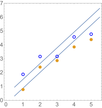
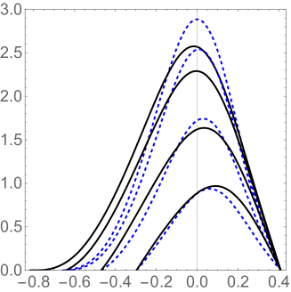
Figure 6: Upper: Squared masses of the Delta (open points) and N (closed) resonances versus their successive quantum number $n$. The two straight lines shown for comparison, are the Regge trajectories fitted to the experimental values of $M^{2}(J)$ , versus the total angular momentum $J$, with the slope $\alpha^{\prime}=0.88\,GeV^{2}$.
Lower: LFWFs for the lowest Delta (dashed lines) and N (solid lines). The plots are shown versus the Jacobi coordinate $\lambda$, for fixed $\rho=0,0.1,0.2,0.3$, top to bottom.

Recall that these masses are calculated from limited basis set, with only 12 longitudinal eigenfunctions of the Laplacian. Also note, that neither the perturbative Coulomb nor the spin-dependent interactions are included. The Delta-N splitting is due only to the ’t Hooft operator treated in a quasi-local approximation.

The lower part of the plot shows the light front wave functions of the lowest mass $\Delta$ and $N$ baryons. The attractive and quasi-local interaction makes the wave function of the nucleon $N$ wider than that of the isobar $\Delta$, i.e. greater both at the left and right side of the plot (corresponding to $x_{d}\rightarrow 1$ and $x_{d}\rightarrow 0$.). This widening effect is similar to that observed for mesons. The LFWF of vector mesons is relatively narrow, while that of the pion is nearly flat. Furthermore, as $d$ participates in two pairings while each $u$ only in one, this effect is more pronounced for the $d$ quark.

VII Baryon formfactors

In the non-relativistic formulation, the formfactors are defined as overlap integrals. This carries to the light front, with the formfactors as overlap of the LFWFs. In particular the helicity preserving Dirac formfactor is Drell and Yan (1970); West (1970); Lepage and Brodsky (1980)

$$F_{1}(q^{2})=\langle\vec{P}+\vec{q},\uparrow|J^{+}/2P^{+}|\vec{P},\uparrow\rangle$$ (43)

To evaluate (43), we select the momentum transfer to be $q$ in the transverse x-direction, and select the struck quark to be number 3 ($d$ quark). More specifically, the transverse momenta in the struck baryon (with prime) are related to those in the non-struck one (without prime) by

$$k^{1^{\prime}}_{x} = k^{1}_{x}-x_{1}q,\,\,k^{2^{\prime}}_{x}=k^{2}_{x}-x_{2}q,$$

$$k^{3^{\prime}}_{x} = k^{3}_{x}+(1-x_{3})q$$ (44)

The three transverse momenta $\vec{k}^{i}$ and longitudinal fractions $x_{i}$ need to be re-expressed in terms of two Jacobi momenta, in our notations $\vec{p}_{\lambda},\vec{p}_{\rho}$ and $\rho,\lambda$, on which LFWFs depend.

For illustration, let us take the example of a LFWF with a Gaussian transverse momentum dependence. For the struck LFWF it takes the form

$$exp\big{(}-A\sum_{1}^{3}(\vec{k}^{i^{\prime}})^{2}\big{)}\rightarrow exp\big{(}-A\big{[}\vec{p_{\lambda}}^{2}+\vec{p_{\rho}}^{2}-{2\over 3}(\vec{p_{\lambda}}\cdot\vec{q})(\sqrt{6}+3\lambda)-2(\vec{p_{\rho}}\cdot\vec{q})\rho+\vec{q}^{2}(2+2\sqrt{6}\lambda+3\lambda^{2}+3\rho^{2})/3\big{]}\big{)}$$ (45)

Selecting the momentum units such that $A=1$, and convoluting it with various longitudinal wave functions (defined as always on the equilateral triangle), we can see how the formfactor depends on their shape. In Fig.7 we present results of LFWF convolution, for two extreme cases: “Neumann" wave function flat (constant) on the physical triangle, and “Dirichlet" wave function $\psi\sim x_{1}x_{2}x_{3}$ satisfying linear boundary conditions on all sides of the equilateral triangle. As expected, the Neumann wave function with sharper edges, produce a larger formfactor at large $q^{2}$, although the overall difference is not that large. Note that this methodical example (not expected to be realistic) is well reproduced by the dipole form $1/(1+C^{2}q^{2})^{2}$, by which the nucleon formfactors were originally fitted decades ago.

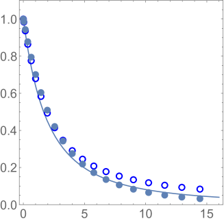
Figure 7: The formfactors for ‘Neumann" (open points) and “Dirichlet" (closed points) wave functions defined in the text, versus the momentum transfer $q^{2}$.A line, shown for comparison, corresponds to the dependence $1/(1+q^{2}/4)^{2}$.

We now show the formfactors calculated with the longitudinal wave functions for the Delta and Proton, following from our analysis in the preceding section. In order to see better the most interesting region of large $q^{2}$, we plot $Q^{4}F_{1}^{d}(Q^{2})$ in Fig.8.

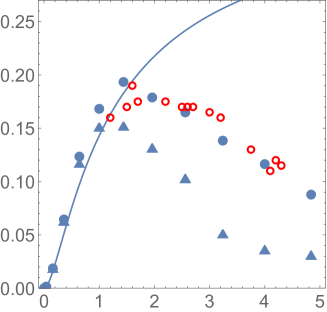
Figure 8: $Q^{4}F_{1}^{d}(Q^{2}),\,(GeV^{4})$ versus the momentum transfer $Q^{2}\,(GeV^{2})$. The triangles and closed points correspond to the Delta and Proton LFWFs, respectively. The red circles are extraction from the experimental data on the $p$ and $n$ formfactors mentioned in the text. The solid line shown for comparison, corresponds to the dipole form factor $Q^{4}/(1+Q^{2}/m_{\rho}^{2})^{2}$.

Experiments are of course done with protons and neutrons, but using them one can extract separate formfactors for $u$ or $d$ quarks. This was done e.g. in Qattan and Arrington (2012), and the red circles in Fig.8 are from Fig.8 of this work. (For clarity we do not show the datapoints in the range $Q^{2}<1\,GeV^{2}$, as the error bars for these points are $\pm 0.02$ on average.) From the plot, we see that this formfactor does not appear to reach a constant limit at large $Q^{2}$, with the measured points slowly decreasing towards the right hand side. Old dipole parametrization $Q^{4}F=Q^{4}/(1+Q^{2}/m_{\rho}^{2})^{2}$ asymptotes a constant at large $Q^{2}$ from below.

Remarkably, our longitudinal proton wave functions convoluted with (45) reproduces such a trend, and (with the parameter $A=4\,GeV^{-2}$ ) they follow the shape indicated by the data rather well. The calculated formfactor for the case when the struck quark is $u$ has a similar shape. Unfortunately, according to Qattan and Arrington (2012), the experimental trend is different, the constant at $Q^{2}\rightarrow\infty$ is approached from below. By the Drell-Yan relation this flavor difference is also seen in the PDFs of $u$ and $d$ at $x\rightarrow 1$. Flavor asymmetry must be related with the asymmetry of the spin-orbit part of the wave function, which in our approximations is so far ignored.

Note that the corresponding formfactor for Delta (triangles) is significantly softer, as one would expect from the size of the wave function. Recall that the large difference between the Delta and Proton formfactors (so well seen in this plot) is completely due to the ’t Hooft quasi-local pairing $ud$ interaction. While we do not have Delta targets for experiments, perhaps its formfactor can be calculated on the lattice, or in other models.

Let us now make a more general comment on possible improvements of the LFWFs calculated in this work, and in particular their consequences for formfactors at large $Q^{2}\rightarrow\infty$ and PDFs at large $x\rightarrow 1$. We treated light quarks as “constituent quarks" with fixed mass $M\sim 400\,MeV$ everywhere, including the “cup potential" $\sim M^{2}/x$ diverging at kinematical edges. As a result, our LFWFs vanish at these edges in a smooth way. However it is known that $M^{2}$ decreases with virtuality of the quark and vanishes if it is highly virtual. The instanton-based theory of chiral symmetry breaking shows how it is related to the instanton zero modes and describe smooth transition from on-shell constituent quarks to near-massless quark-partons. We are planning to include this effect in subsequent works.

Completing the section on formfactors and trying to avoid any confusion, let us comment on the relation between our results and those in the literature on “hard regime" $Q^{2}\rightarrow\infty$ limit. These terminology is used in literature in very different settings. One is physics of heavy boson or quark production $W,Z,H,t$ or jet observables at colliders: here $Q^{2}\sim(100\,GeV)^{2}$ and pQCD is fully accountable for those.

A completely different situation is with $exclusive$ processes, such as elastic scattering and formfactors. Specific powers of $1/Q^{2}$ and powers of $\alpha_{s}(Q^{2})$ follow from the lowest orders pQCD diagrams Brodsky and Farrar (1973). Furthermore, in some cases (e.g. the pion formfactor) even the constant in the hard limit can be expressed in terms of $f_{\pi}$, so the pQCD asymptotic prediction is fully known. It is further known for decades, that in the “semi-hard" domain of current experiments $Q^{2}<10\,GeV^{2}$ the formfactors are $not$ dominated by pQCD mechanisms. In our paper on formfactors Shuryak and Zahed (2021d) we included the instanton contributions in the hard blocks. While important in the “semi-hard" domain, at large $Q^{2}$ those become exponentially small $\sim exp(-Q\rho)$ at $Q\rho\gg 1$. In this series of papers, we used the ’t Hooft Lagrangian as a $quasi-local$ operator. This means the opposite regime, where the distance scales considered are $large$ compared to the instanton size $\langle r\rangle\gg\rho$.

VIII Bridging the gap between hadronic and partonic dynamics

VIII.1 The matching scale

Before building a bridge, one should have a good assessment of both sides of the river. Therefore let us start with a brief summary of what we know on the two extremes.

Since the 1970’s we know that hard processes defined at some high scale $Q^{2}\gg 1\,GeV^{2}$ can be described as a set of independent “partons", $g,q,\bar{q}$. The probabilities to find those in a target (or beam) hadrons are known as PDFs $q(x,Q^{2})$. Due to high resolving power in this regime, the pointlike quark-partons and gluons can emit each other with “splitting functions" following directly from the QCD Lagrangian. So PDFs and structure functions at different Q are related by perturbative DGLAP “evolution". Combining these with fits to experimental data on various partonic processes, has mushroomed into a large body of work. For a recent summary see e.g. reviews by CTEQ collaboration such as Hou et al. (2021).

(While the partonic PDFs definitely represent a very solid end of the bridge, they are not constructed without certain approximations. Subsequent gluon emissions are assumed to be incoherent, i.e. the DGLAP equations are probabilistic kinetic equations. As noted in Kharzeev and Levin (2017), this assumption generates an entanglement entropy. However, hadrons are pure states, and their consistent treatment should be based on their complete LFWFs, without entanglement.)

By evolving DGLAP to sufficiently low normalization point, one finds a scale at which gluons can no longer be emitted. The lowest glueball masses have a mass scale $M_{glueballs}\sim 2\,GeV$, and so a crude estimate for ithis limiting scale is the gluon effective mass $M_{eff}(gluon)\sim 1\,GeV$. We expect the lower end of the DGLAP evolution to be located at $Q^{2}\sim M_{eff}(gluon)^{2}$.

On the other side (lower $Q^{2}$), chiral symmetry breaking puts special emphasis on the lightest mesons, the Nambu-Goldstone modes – the pions – and the condensate $\sigma$. Instead of the QCD Lagrangian, one has a chiral effective Lagrangian and its higher order descendants. Its $upper$ cutoff scale can be identified with the original cutoff of the Nambu-Jona-Lasinio (NJL) model $\Lambda_{\chi}\sim 1\,GeV$. Later its mechanism was related to $instantons$ Shuryak (1982), and this cutoff with the typical instanton size $\rho\sim 1/3\,fm$.

So, our preliminary assessment suggests a nice plan for a bridge, with a hope that its “arcs" – the chiral and the pQCD ones – will join relatively smoothly at the $1\,GeV$ scale. In this section we are going to investigate if the PDFs evaluated from both sides do indeed join there. (Needless to say, there are many other observables for which one may need more sophisticated strategy than a jump from one theory to another. Here, we would like to emphasize the efforts by many, to include both perturbative and nonperturbative effects, among which our own discussions of meson formfactors in Shuryak and Zahed (2021d), and spin-dependent forces in Shuryak and Zahed (2021a) .)

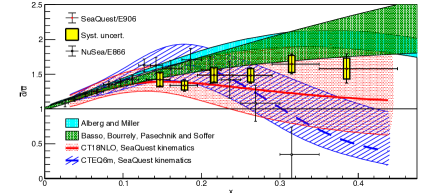
Figure 9: Flavor asymmetry of the antiquark sea as the ratio of PDFs of $\bar{d}/\bar{u}$ versus $x$ Dove et al. (2021).

In Fig.1 we illustrate the processes affecting the PDFs . Perturbatively, an extra $\bar{q}q$ pair can be mediated by virtual gluons, see (a,b). Since gluons are “flavor blind", they produce $\bar{u}u,\bar{d}d$ in equal number. Another process shown in Fig.1 (c,d) uses the instanton-induced ’t Hooft four-fermi interaction in the production channels. As first noted in Dorokhov and Kochelev (1993), it is “maximally flavor antisymmetric" due to the Pauli principle for instanton zero modes of fermions. Also, since there are two $u$ and one $d$ valence quarks, in the first order in this mechanism the simple prediction for antiquark flavors would be

$${\bar{d}\over\bar{u}}\rightarrow 2$$ (46)

And for $\Delta^{++}$ with valence $uuu$ only, the sea should consists of only $\bar{d}$, without $\bar{u}$!

The flavor asymmetry of the sea is a very convenient tool to discriminate what part of the “sea" (multiparticle/multiparton sectors of the LFWFs) come from chiral (step 2) processes and which from pQCD (step 3), because it can only come from the former.

VIII.2 Phenomenology of the nucleon antiquark sea

Let us now briefly describe what is known about the flavor asymmetry of the antiquark sea. First discovered as “violation of Gottfried sum rule" (an assumption that the sea is produced entirely by gluons) three decades ago, it is still being developed. For reference, at $4\,GeV^{2}$ scale, the NMC collaboration found

$$\int_{0}^{1}dx\big{(}\bar{d}(x)-\bar{u}(x)\big{)}=0.147\pm 0.039$$ (47)

Indeed, experiments have shown a surprisingly strong violation. The NuSea experiment Towell et al. (2001) gives for this ratio $\approx 1.5$ at $x\sim 0.2$. The more recent SeaQuest experiment Dove et al. (2021), has found that the asymmetry persists to larger momentum fractions, at least up to $x\sim 0.4$, see Fig.9 (copied from Dove et al. (2021)). Also shown in this figure, are the CT parameterizations of the previous data, the so called MMHT14 PDF polynomial parameterization Basso et al. (2016), and some theoretical predictions. Ref Alberg and Miller (2019) (green strip) uses a model based on the “pion cloud" of the nucleon ( see also Alberg et al. (2022)).

In Fig. 11 we show the difference $\bar{d}(x)-\bar{u}(x)$ as a function of $x$ from NuSea/866 experiment. It shows that the effect is localized at $x<0.2$, but strongly $grows$ towards small $x$.

Having briefly reviewed the experimental situation, let us outline the related theory efforts. The LF wave functions of the baryons ($\Delta$ and $N$) with the $five-quark$ sector was studied in Shuryak (2019). This paper included the four-quark ’t Hooft interaction to first order, and obtained antiquarks PDFs from rather complicated wave functions. Its overall shape and scale reproduced the data shown in Fig.11. Yet there were visible oscillations, coming perhaps from the rather limited functional basis set used.

VIII.3 The $q\bar{q}$ pair production, to the first order in ’t Hooft Lagrangian

The first study of the five-quark sector of the baryon wave functions has been done by one of us in Shuryak (2019). In it the diagrams Fig.1 (c) or (d) were used to calculate the matrix of basis matrix elements relating 3- and 5-q states, and the Hamiltonian was then diagonalized. This procedure includes diagrams of all orders. However, the set of basis states used in that paper was based on a nonlinear map of momentum fractions $x_{i}$, from 5 to 4, and the procedures was rather complicated.

In fact, there is no need to follow this path, as the (modified) Jacobi coordinates provide a linear map. The physical domain of the 5 momentum fraction with a condition $\sum_{1}^{5}x_{i}=1$ is the 4-d manifold called $pentachoron$ (or 5-cell or or 4-simplex), which is one dimension higher than tetrahedron. For the case of 5 quarks such map is detailed in Appendix D. The four coordinates $\alpha,\beta,\gamma,\delta$ play the same role as $\rho,\lambda$ for three quarks. We conjecture that the eigenstates of the Laplacian on the 5-simplex can also be worked out analytically using some set of standing waves, see Shuryak and Zahed (2021c) for discussion and for the ground state in this form.

The PDF is the integral of the squared wave function projected onto a $single$ variable of the set. For $N$ constituents with $N-1$ Jacobi coordinates, the integral has dimension $N-2$, by tracing over the coordinates called generically $"\rho"$

$$PDF("\lambda")=\int d^{N-2}"\rho"|\psi("\rho","\lambda")|^{2}$$ (48)

If for a crude estimate we take the wave function be flat over the manifold, then $PDF(x)\sim(1-x)^{N-2}$. For $N=3$ the power is linear, while for $N=5$ it is a cube.

In this work we carry all the way to the evaluation of the 5-q LFWF in Jacobi coordinates. Instead, we provide some estimates of the probability of the process to lowest order in the ’t Hooft vertex. It follows the same spirit as DGLAP treatment of extra gluons and sea quarks. More specifically, the interaction among the emitted quarks is ignored, motivated by the observation that the kinematical domain for the newly produced quarks correspond to $x$ much smaller than those of the valence quarks. So, their production is treated as in free space, by a diagram with free phase space integration.

Let us denote by $A_{1}$ the amplitude of the $q\bar{q}$ pair production in the first order in the ’t Hooft vertex, corresponding to diagrams Fig.1 (c) or (d). Since it uses a process with fermionic zero mode of the instanton, it should be proportional to a small instanton packing fraction $\kappa=(\pi^{2}/2)\rho^{4}n_{I+\bar{I}}\sim 1/10$ of the original Instanton Liquid Model which sets the order of magnitude of the effect.

All u- and d-quark emissions yield the final states

$$u\rightarrow A_{1}^{2}\,u+A_{1}^{2}(d+\bar{d})$$

$$d\rightarrow A_{1}^{2}\,d+A_{1}^{2}(u+\bar{u})$$ (49)

If we note that the probability for a quark to do nothingh is $1-A_{1}^{2}$, then the proton composition after one interaction is

$$(2+A_{1}^{2})u+(1+2A_{1}^{2})d+A_{1}^{2}\bar{u}+2A_{1}^{2}\bar{d}$$ (50)

which is valence quark preserving with $u_{v}=u-\bar{u}=2$ and $d_{v}=d-\bar{d}=1$. The parton distribution for the neutron follows by isospin symmetry. In this schematic description of the proton and neutron sea contributions to first order in $A_{1}^{2}$, the Gottfried sum rule reads

$$\frac{1}{3}+\frac{2}{3}(\bar{u}-\bar{d})=\frac{1}{3}-\frac{2A_{1}^{2}}{3}\rightarrow 0.227$$ (51)

More specifically, the simplified and ultra-local’t Hooft vertex

$$G_{tHooft}({\rm det}(\overline{q}_{R}q_{L})+{\rm det}(\overline{q}_{L}q_{R}))$$ (52)

reduced to $u,d$ flavors, is characterized by the coupling

$$G_{tHooft}\approx 35\,GeV^{-2}$$ (53)

see the related discussion in Appendix E. For the process

$$u(K_{u})\rightarrow u(K_{\underline{u}})+d(K_{d})+\bar{d}(K_{\bar{d}})$$ (54)

we define the 4-momenta in the infinite momentum frame as

$$K_{u} = (P,P,0_{\perp})$$

$$K_{d} = (xP+\frac{\vec{k}_{\perp}^{2}}{2xP},xP,\vec{k}_{\perp})$$

$$K_{\bar{d}} = (zP+\frac{p_{\perp}^{2}}{2zP},zP,p_{\perp})$$

$$K_{\underline{u}} = ((1-x-z)P+\frac{(\vec{p}_{\perp}+\vec{k}_{\perp})^{2}}{2(1-x-z)P},$$ (55)

$$(1-x-z)P,-(\vec{p}_{\perp}+\vec{k}_{\perp}))$$

Assuming the produced $\bar{d}$ in an unpolarized $u$, we calculate the $probability$ of the process as a square of the amplitude defined by old-fashion perturbation theory

$$dN_{\bar{d}/u}= \frac{G^{2}_{tHooft}}{2}\frac{\overline{|V_{u\rightarrow ud\bar{d}}|^{2}}}{(E_{u}-E_{\underline{u}}-E_{d}-E_{\bar{d}})^{2}}$$ (56)

$$\times\frac{1}{2E_{u}}\frac{1}{2E_{\bar{d}}}\frac{1}{2E_{\underline{u}}}\frac{1}{2E_{d}}\frac{d^{3}K_{\underline{u}}}{(2\pi)^{3}}\frac{d^{3}K_{d}}{(2\pi)^{3}}$$

with the energy denominator, and the bar on the matrix element refers to spin averaging over the’t Hooft vertex. In the vertex there are terms proportional to constituent quark masses squared $m_{q}^{2}$ and to momenta squared $\vec{p}^{2}$. As we will show in more detail in Appendix  F, the momenta are regulated by the instanton formfactors and therefore $\vec{p}^{2}\sim 1/\rho^{2}$. For simplicity we have ignored all terms with masses because $(\rho m_{q})^{2}\sim 1/4$ can be considered small. With this in mind, the spin averaging gives

$$\overline{|V_{u\rightarrow ud\bar{d}}|^{2}}=\frac{1}{2}16(K_{u}\cdot K_{\underline{u}})\,(K_{d}\cdot K_{\bar{d}})$$ (57)

with (56) taking the form

$$dN_{\bar{d}/u}=\frac{G_{tHooft}^{2}}{4}\,\bigg{[}\frac{\frac{(\vec{k}_{\perp}+\vec{p}_{\perp})^{2}}{2(1-x-z)}[\frac{\vec{k}_{\perp}^{2}}{2x}+\frac{\vec{p}_{\perp}^{2}}{2z}+(1-\frac{1}{x+z})\frac{(\vec{k}_{\perp}+\vec{p}_{\perp})^{2}}{2(1-x-z)}](x+z)}{(\frac{\vec{k}_{\perp}^{2}}{2x}+\frac{\vec{p}_{\perp}^{2}}{2z}+\frac{(\vec{k}_{\perp}+\vec{p}_{\perp})^{2}}{2(1-x-z)})^{2}}\bigg{]}\frac{1}{z}\frac{dx}{x}\frac{dz}{(1-x-z)}\frac{d^{2}\vec{k}_{\perp}}{(2\pi)^{3}}\frac{d^{2}\vec{p}_{\perp}}{(2\pi)^{3}}$$ (58)

The sea distribution of $\bar{d}$ in an unpolarized constituent quark $u$, is given by

$$N_{\bar{d}/u}(z,Q^{2})=\int_{p_{\perp}}\int_{\vec{k}_{\perp}}\int_{x}\,\frac{dN_{\bar{d}/u}}{dz}$$ (59)

with the integrals carried sequentially in the ranges: $0\leq x\leq 1$ and $0\leq p_{\perp}^{2}\leq Q^{2}$. The sea distribution $\bar{u}$ in an unpolarized constituent quark $d$, is identical with $dN_{\bar{d}/u}=dN_{\bar{u}/d}$. For its evaluation see Appendix F. Using the value of the coupling of the ’t Hooft operator (53), one finds the probability of the process $A_{1}^{2}\approx 0.11$, which sets the scale of the “primary sea" produced by $1\rightarrow 3$ instanton-induced process. (The regulator on which the dependence is logarithmic, is taken to be $\epsilon=0.01$.)

The next issue we address is the $shape$ ($x$-dependence) of the PDFs of these sea (anti)quarks produced by the processes in Fig. 1 (c,d). Those can be obtained by convolution of this squared amplitude, treated as a “splitting function" with the original (valence) distributions $d^{N}(y),u^{N}(y)$ (e.g. those calculated from the LFWFs in the 3-q sector above). The unpolarized sea $\bar{u},\bar{d}$ distributions in the nucleon are then

$$\bar{u}_{N}(x,Q^{2}) = \int_{x}^{1}\frac{dy}{y}\,d^{p}(y,Q_{0}^{2})N_{\bar{u}/d}\bigg{(}\frac{x}{y},Q^{2}\bigg{)}$$

$$\bar{d}_{N}(x,Q^{2}) = \int_{x}^{1}\frac{dy}{y}\,u^{p}(y,Q_{0}^{2})N_{\bar{d}/u}\bigg{(}\frac{x}{y},Q^{2}\bigg{)}$$

where $q^{p}(x)$ is the unpolarized flavor $f=u,d$ distribution in a proton $p$, at the low resolution point which we argued above is $Q_{0}^{2}\approx(2/\rho)^{2}$. In Fig.10 we plot the $ratio$ of the produced sea PDF to the one which initiated it, $\bar{d}^{N}(x)/u^{N}(x)$. The sea is strongly shifted to small $x\sim 1/10$. At large $x$, if the initial PDF $u^{N}(x)\sim(1-x)^{a}$ has a certain power $a$, the produced one has power $a+1$. (While both these features are clearly steps in the right direction, the reader is perhaps aware that the observed sea PDF have at small $x$ negative power singularities, and a much larger difference between powers of $(1-x)$ in $u^{p}(x)$ and $\bar{d}^{p}(x)$, being approximately 3 and 7, respectively. These features however are known to be generated by subsequent DGLAP evolution from $Q_{0}$ to the the scale $Q$ at which experiments are done.)

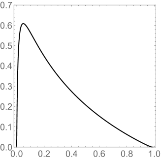
Figure 10: The ratio of the “produced" sea PDF to the one which initiated it $\bar{d}^{N}(x)/u^{N}(x)$ as a function of $x$ following from (VIII.3).

VIII.4 The sea induced by the “pion cloud"

The “pion-induced" contributions to the PDFs, see Fig.1 (e,f) (written in DGLAP-like form), were proposed in Eichten et al. (1992) three decades ago. Note that the $\pi^{0}$ diagrams (e) for the specific in and out quark pairs have a factor of $(1/2)^{2}$, while the $\pi^{+}$ diagram (f) leads to flavor transition $u\rightarrow u\bar{d}$ with a larger factor $1$. The former changes the flavor of the recoil quark, but the latter does not. Because these two diagrams have different probabilities, they together lead also to a flavor asymmetry of the sea. Note that these pion-induced diagrams can also be considered to be higher order iterations of the ’t Hooft vertex, in different channels.

Here we evaluate the contribution of the pion-induced antiquark production, following Eichten et al. (1992): Let the probability of the pion-generated pair production process be $P_{\pi}$, then all valence $uud$ quarks together produce a sea with probability $P_{\pi}(7/4\bar{u}+11/4\bar{d})$, or

$${\bar{d}\over\bar{u}}={11\over 7}\approx 1.57$$ (61)

which is in good agreement with the ratio reported experimentally. Using the absolute observed magnitude of $\bar{d}-\bar{u}$ (47), one finds that in order to explain its integrated magnitude one would need $P_{\pi}\approx 0.2$.

The expression for $P_{\pi}$ from the chiral Lagrangian Eichten et al. (1992) (20, contains the following dimensionless combination of pion constants (in their notations)

$${g_{a}^{2}m_{q}^{2}\over 8\pi^{2}f_{\pi}^{2}}\approx 0.09$$ (62)

times certain integral being $O(1)$ (mildly depending on upper cutoff $\Lambda_{chiral}$. As a result, $P_{\pi}^{th}$ given by the pion diagrams gives about $half$ of the empirical effect.

In summary, we conclude that the first-order in the ’t Hooft interaction, and the iterated (pion) diagrams give comparable contributions to integrated flavor asymmetry of the antiquark sea. Unfortunately, at this time it is not possible to make a more quantitative evaluation including both.

The next question is how the antiquarks produced by the intermediate pions are distributed in $x$. For that we adopt the expression (18) in Eichten et al. (1992), using the convolution of the quark PDFs in the nucleon $q^{N}(y)$ with the “splitting function" $P(z)$, followed by a convolution with the pion PDF $q^{\pi}(x/yz)$. Unlike Eichten et al, however, we do not use here the PDFs fitted from experiments at some high $Q^{2}$, since our intensions here is to build another –chiral – ark of the bridge. So we take $q^{N}(y)=12y(1-y)^{2}$ (approximately corresponding to the wave functions derived for three quarks with the quasi-local attraction above). We also take the symmetric PDF for the pion $q^{\pi}(x)=6x(1-x)$ corresponding to a two-quark semicircular wave function. Convoluting those with the “splitting function" $P(z)$, we get the shape of the pion-induced antiquark PDF shown in Fig.11 (lower). As one can see by comparing it to the upper experimental plot, it does reproduce the observed shape quite well.

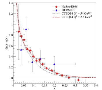
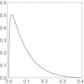
Figure 11: Upper: the difference of sea antiquark PDFs $\bar{d}(x)-\bar{u}(x)$ from experiments. Lower: the calculated shape of sea antiquark distribution (arbitrary units) described in the text.

Finally, let us briefly discuss the issue of flavor asymmetry of valence quark distribution. The empirical PDFs are such that $(u_{v}(x)/2d_{v}(x)>1$ at large $x\rightarrow 1$. As was explained in section VI, the quasi-local pairing interaction makes the LFWFs “flatter" (larger at large x) and, since the $d$ quark in the proton participate in two of those, one finds the opposite, $(u_{v}(x)/2d_{v}(x)<1$ at $x\rightarrow 1$. However, chiral processes leading to the sea quark production work in the opposite direction, towards the one observed. Let us single out the last diagram (f) of 1 with an intermediate $\pi^{+}$. (Its contribution is larger than diagram (e) with $\pi^{0}$ by a factor 4, the flavor factors.) It interchanges the flavors of the leading quarks: if the original one is $u$ (as shown in this figure) then the recoil one – the one at larger x – is $d$.

VIII.5 Evolution down to the matching point

The PDFs describing the experimental and lattice data are professionally fitted to certain analytic forms, and connected to each other via perturbative DGLAP evolution. For definiteness, we will rely on a sufficiently complete global fit called CTEQ18, in Ref Hou et al. (2021), Appendix C. It is defined at $their$ lowest scale

$$Q^{2}_{CTEQ}\approx 1.7\,GeV^{2}$$

The reason we need to discuss it at the end of this paper, is that we are going to evolve it further down, to the matching point discussed in section VIII.1.

We would not repeat those expressions here, just show their plot for valence quarks and gluons in the proton in Fig.12. Unlike many other similar plots, we have not reduced the gluons by any artificial factor, to fit it better in the plot. Our aim is to remind the reader that, even at this scale $Q^{2}_{CTEQ}$, the proton contains significant amount of glue. In fact, as is obvious from the plot, they are dominant at $x<0.2$. Integrating these curves, one gets the corresponding momentum fractions at scale $Q^{2}_{CTEQ}$, $\langle x_{g}\rangle=0.385,\langle x_{uv}\rangle=0.325,\langle x_{dv}\rangle=0.134$. So, at this scale gluons are by no means subleading.

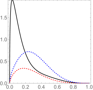
Figure 12: CTEQ18 PDFs of the gluons $xg(x,Q^{2}_{CTEQ})$ (black solid curve), valence up $xu_{v}(x,Q^{2}_{CTEQ})$ and down $xu_{v}(x,Q^{2}_{CTEQ})$ quarks (blue and red dashed curves.

We have recalled these details to stress once more that the scale $Q^{2}_{CTEQ}$ is not low enough to match to the hadronic spectroscopy. Indeed, it operates in terms of constituent quarks and have no gluons. So, what happens with the gluons when one performs DGLAP evolution $downward$, say to our “matching scale" $1\,GeV^{2}$?

Despite the fact that the amount of corresponding "DGLAP evolution time" is not long, $log(Q^{2}_{CTEQ}/Q_{matching}^{2})\approx 0.52$, dramatic changes take place for the gluons. Using the lowest order splitting function

$$P_{gg}(z)=6\bigg{(}{z\over 1-z}+{1-z\over z}+z(1-z)\bigg{)}$$

convoluted with $CTEQ18$, we have evolved the gluons downward to our “matching scale": the results are shown in Fig.13. As expected, we see the gluons (and in particular $\langle x_{g}\rangle$) practically disappear! (Except at small $x$ where $g(x)$ gets negative, which of course makes no sense.) Oviously, the same downward evolution increases $u,d$ momentum fractions roughly to $2/3,1/3$.

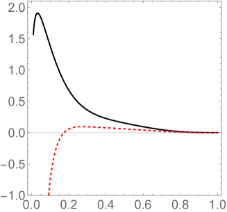
Figure 13: Black solid line is the CTEQ18 gluon distribution $xg(x,Q^{2}_{CTEQ})$, and red dashed line is its version evolved downward by DGLAP to $Q_{matching}^{2}=1\,GeV^{2}$.

Furthermore, the same perturbative downward evolution practically erases the quark-antiquark sea at the matching scale. However, what is left there is the sea generated by chiral dynamics, as discussed in the two preceding subsections, generating observable flavor asymmetry of the antiquarks. Note further that the mean momentum fractions $\langle x_{\bar{q}}\rangle$ generated there, are at about 2-3 % level, and of course they are complemented by the gluon-generated sea at higher scale.

The use of DGLAP in this section is by necessity very crude. The analysis can be improved, to make our “bridging the gap" goal smooth. It should eliminate artifacts (like negative PDFs) authomatically. Some modifications are rather obvious, e.g. the inclusion of quark and gluon masses in the splitting functions. Others may include the transition from kinetic equations to LFWFs.

IX Summary

This is the concluding paper of the series of five papers, and it is fitting to briefly overview here the main goals and results of the whole program, with some specifics about each of them.

When starting this program we had two general goals:
(a) One was to bring the quark models used in hadronic spectroscopy to the light front.
(b) The other was to connect the obtained LFWFs to partonic observables as deduced from various hard scattering processes.

The first goal is basically accomplished. Somewhat unusual, the LF Hamiltonians create technical problems, but those were solved. We have shown how one can include the confining forces and solve the corresponding Schroedinger equation for mesons and for baryons (“on equilateral triangle"). This construction reproduces the masses of multiple lowest states in each channel, with agreement with empirical Regge trajectories. We also were able to include the “residual" quasi-local binary attraction in a nonperturbative way, describing “good diquark" correlations in a nucleon. Of course, a lot of work remains to be done, such as the inclusion of the spin-depend potentials and the mixing between the various spin-orbit components of the wave functions. Clearly, this can be done in a relatively straightforward way.

The second goal is accomplished only partly. By adding the 5-quark sector to baryons via certain approximate methods of chiral dynamics, we found a reasonable magnitude of the antiquark sea, as well as its distribution in $x$. The observed flavor asymmetry of the sea is explained.

However matching the experimental data on the PDFs, DAs, GPDs etc at high scale, to those we calculated from the LF wave functions at low scale, can so far be done only at the level of average quantities, e.g. $\langle x_{q}\rangle$ but is not yet quantitative for their $x$-dependence. We attempted to bring downward the DGLAP to a scale as low as 1 $GeV^{2}$, where we see that $\langle x_{g}\rangle\rightarrow 0$. However, we need to tweek the DGLAP evolution to accomodate switching off the gluons in a consistent manner. Also this probabilistic description is only justified when $x$ of the produced partons is small compared to that of their parents, for otherwise we need to develop a coherent Hamiltonian description for the quark-gluon sector.

This is now a good place, to remind the reader for the specific content of these five papers. We started in the first paper Shuryak and Zahed (2021a) with discussion of the physical origin of the confining and spin-dependent potentials for heavy quarkonia in a traditional setting, in which they are defined via some correlators involving Wilson lines. Specifically, we focused on instanton-induced effects. Following our earlier paper on mesonic formfactors Shuryak and Zahed (2021d), we did so in a novel “dense instanton liquid" which includes both instantons forming the quark condensate (a subject of studies in the previous four decades) and close instanton-antiinstanton molecules. We have shown that such a vacuum model reproduces the phenomenological confining potential up to distances of $r\sim 0.8fm$. The spin-dependent potentials are defined via Wilson lines with added magnetic field strengths. The perturbative and instanton-induced effects are both short-range and were shown to have comparable magnitude for charmonia, with instanton effects dominating for light quark systems.

The second paper Shuryak and Zahed (2021b) starts the derivation and usage of the light-front Hamitonians $H_{LF}$ for the description of meson light-front wave functions (LFWFs). Here we developed the “einbine trick", by means of which a potential linear in coordinates turns into a quadratic one. Then, writing the coordinates as derivatives over momenta, we net Laplacian-like confining terms, while the kinetic energy $\sim(p_{\perp}^{2}+m^{2})/x$ is treated as a certain potential energy. The masses of the obtained states were shown to be close to the expected Regge trajectoris, with novel LFWFs to follow. In this paper we also managed to put the instanton-related Wilson lines from Euclidean time into the light cone, by analytic continuation from Euclidean angle to Minkowskian rapidity (the hyperbolic angle). We have derived the spin-dependent terms of $H_{LF}$ following from Wilson lines (nonzero fermionic modes), and ’t Hooft effective Lagrangian (zero modes). The latter was shown to generate massless pion: as a benefit we have its LFWF.

The third paper Shuryak and Zahed (2021c) was also devoted to mesons on the light cone, focusing on spin-spin and spin-orbit forces. Starting with heavy quarkonia (bottomonium), we compared the traditional Schroedinger equation in the CM frame and spherical symmetry, to $H_{LF}$-based approach in which the symmetry is just axial. We do get the correct spectrum of bottomonia, in agreement with its Regge trajectory. Using the fact that $H_{LF}$ has full relativistic kinematics, in which there is no principal distinction between heavy and light quarks, we extended the latter to strange and light mesons. We focused on spin and orbital momentum mixing onthe LF, in which both are represented just by their longitudinal projections. We studied the role of the tensor forces and mixing in vector mesons, generating their quadrupole moments (both in the CM and on the LF frames). At the end, we studied the relations between LFWFs and the PDFs and distribution amplitudes (DAs) of the mesons.

In the fourth paper Shuryak and Zahed (2022) we proceeded to three-quark baryons, with heavy and light quarks. However, in this paper we restricted our analysis to $flavor-symmetric$ baryons ($bbb,ccc,sss,uuu$) in which the ’t Hooft four-fermion effective Lagrangian does $not$ operate. One novel feature was the detailed calculation of the instanton-induced three-static-quark potentials, which were also compared with available lattice data for the same geometries. Our conclusion is that all of them seem to favor the model we call “Ansatz A", half the sum of binary two-quark potentials. Another feature of this work, separating it from others in literature on baryon LFWFs, is that we used (modified) Jacobi coordinates and thus have as many coordinates as necessary, without spurious center-of-mass motion. The longitudinal momentum fractions $x_{1},x_{2},x_{3}$ are then defined on an equilateral triangle in two Jacobi coordinates. The natural basis functions are therefore those of a Laplacian on such triangle. We were able to give analytic form for this set. Solving the full Hamiltonian requires numerical approaches: one of them uses matrices in terms of basis functions, another is a direct numerical solution of 2d Schroedinger-like eqns (provided the transverse and longitudinal motion can be approximately factorized).

Now we summarize the main content of this paper, the fifth in the series. It is devoted to two very different issues. The first is the flavor-asymmetric “good diquarks" $ud,us,ds$ with $J^{P}=0^{+}$ quantum numbers. Multiple phenomenological and lattice results show that those are rather deeply bound, in comparison to two constituent quarks or “bad diquarks" with other $J^{P}$ values. We calculated the LFWFs including the pairing correlations induced by the instanton-induced ’t Hooft operator, in its quasi-local form. (We showed how to do so without fullly Fourier transforming our momentum wave functions into coordinate representation.) We did so for the heavy-light baryons $\Lambda_{c}=cud$ with a single diquark, and the nucleon with its two pairing $ud$ channels. The masses and, most importantly LFWFs of those, were compared to states without “good diquarks", $\Sigma_{c}$ and $\Delta$ respectively. These differences of LFWFs due to quasi-local pairing are found to be rather significant.

The second issue is in fact the underlying reason for why all those paper were written. Two important subfields of hadronic physics – the $spectroscopy$ (done in the rest frame with the wave functions and constituent quarks), and the partonic physics (done in terms of density matrices PDFs and pointlike quarks and gluons on the LF). The previous four papers make the first step, exporting the spectroscopy to the light front. Here we made the second step, by adding to the 3-q baryons “the sea", again using the ’t Hooft four-fermion operator, but now in 1-to-3 channel. One way to do that would be to use Jacobi coordinates for 5-q systems, which we detailed. However, we do not follow this path to calculate the 5-q LFWFs. Rather, we have proceeded a la perturbative DGLAP evolution, treating this Lagrangian to the lowest order, and evaluated the appropriate “splitting function" and probabilty. The higher orders are approximated by “pion cloud" contribution, already known in the literature. We show that these effects do account for flavor asymmetry of the antiquark sea, both in magnitude and in $x$-dependence.

The final point of this paper is “matching" the valence quark and sea PDFs to phenomenological ones. We think that the matching scale should be $Q^{2}\approx 1\,GeV^{2}$, being both the upper scale of chiral (instanton) physics, and the lowest scale at which the gluon components of the PDFs disappear. We show that these three subsequent steps do indeed provide a bridge between spectroscopy and partonic PDFs, in so far at the semi-quantitative level.

Appendix A Variational study of $ss^{\prime}$ diquarks

Starting from diquarks as a spherically symmetric two-quark system in 3d, and $quadratic$ confinement, one is in an oscillator setting, with a Gaussian wave function for the ground state

$$\phi_{0}(r)=\frac{e^{-{r^{2}\over 2\beta^{2}}}}{\pi^{3/4}\beta^{3/2}}$$ (63)

where $r$ is the $relative$ distance between quarks. The r.m.s. distance is $R_{r.m.s.}=\sqrt{3/2}\beta$.

The simplest interaction between $u$ and $d$ quarks is the local form of the ’t Hooft Lagrangian

$$V_{{}^{\prime}tHooft}=-{G_{{}^{\prime}tHooft}\over 2}\delta^{3}(\vec{r})$$ (64)

where the coupling constant is the one in mesonic (pion or $\eta^{\prime}$) channels. The $-1/2$ stems from the Fiertz transformation in the diquark channel, see Rapp et al. (2000) for details. Averaging it over simplified wave function one gets

$$\langle V_{{}^{\prime}tHooft}\rangle=-{G_{{}^{\prime}tHooft}\over 2\pi^{3/2}\beta^{3}}$$ (65)

The Coulomb interaction in the diquark channel, has also half of the strength compared to the mesonic channel $V_{C}(r)=-(2/3)\alpha_{s}/r$. Its average using the same wave function is

$$\langle V_{C}\rangle=-{2\alpha_{s}\over 3}{2\over\sqrt{\pi}\beta}$$ (66)

which for the same $R_{r.m.s.}$ give about $-0.15\,GeV$. (The additional nonperturbative component – instanton gauge fields – will be evaluate later ).

The wave functions dependence on the strength of ’t Hooft coupling is shown in Fig.14. The diquarks get more compact as the pairing strength grows. This effect is nonlinear in binding, and grows stronger.

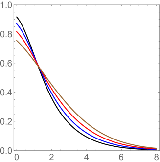
Figure 14: Comparison of the shapes of the wave functions $\psi_{dq}(r)$ vs $r\,(GeV^{-1})$ for $ss^{\prime}$ diquarks, for $G_{qq}=30,20,10,0\,GeV^{-2}$, black, blue, red and brown curves, respectively.

Appendix B From the wave functions in momentum representation to local and Coulomb interactions

The generic two-body interaction, assumed to be between $u$ and $d$ quarks, is of the form

$$\langle V\rangle=\int d^{3}\vec{r}_{u}d^{3}\vec{r}_{d}|\psi_{u}(\vec{r}_{u})\psi_{d}(\vec{r}_{d})|^{2}V(|\vec{r}_{u}-\vec{r}_{d}|)$$ (67)

with a potential depending on the relative coordinate $r_{ud}=|\vec{r}_{u}-\vec{r}_{d}|$, while the WFs depend on the individual coordinates. The average of the local potential (64) takes the form

$$\langle\delta^{3}(\vec{r}_{u}-\vec{r}_{d})\rangle=$$

$$\int d^{3}r_{u}d^{3}r_{d}|\psi(\vec{r}_{u})|^{2}|\psi(\vec{r}_{d})|^{2}\delta^{3}(\vec{r}_{u}-\vec{r}_{d})=\int d^{3}r|\psi(\vec{r})|^{4}$$

familiar in few-body physics, with the 4-th power of the single-body wave functions in the CM frame.

In order to use a more general potential, it us customory to proceed to the momentum representation via Fourier transform $\psi(\vec{r})\rightarrow\psi(\vec{p})$, and introduce the so called overlap function

$$S(\vec{q})=\int{d^{3}p\over(2\pi)^{3}}\psi^{*}(\vec{p})\psi(\vec{p}+\vec{q})$$ (69)

In these notations, the interaction (67) can be rewritten as a convolution of overlap functions squared with the Fourier transform of the potential

$$\langle V\rangle=\int{d^{3}q\over(2\pi)^{3}}|S(\vec{q})|^{2}V(q)$$ (70)

For color Coulomb interaction between quarks $V(q)=(2/3)\alpha_{s}/q^{2}$. This approach is so-to-say $t$-channel description of scattering.

Now, the difficulty we have is related to the fact that the LFWFs are defined in momentum representation, while the binary interactions is given in coordinates. However, since the ’t Hooft interaction can be approximated by a local form (21), we can avoid the cumbersome Fourier transforms, and use an alternative $s$-channel description without oscillating exponents.

Let us explain it first using the simplest example of a meson. In this case the wave function is a function of the relative coordinates $\vec{r}=\vec{r}_{1}-\vec{r}_{2}$ already, so the local interaction is just proportional to the coordinate wave function at the origin $-G|\psi(\vec{r}=0)|^{2}$. (For example, such an approximation is in fact exact for perturbative spin-spin interactions, in atoms, nuclei and baryons.) The point is that it has a simple expression in terms of the wave function in momentum representation

$$\psi(\vec{r}=0)=\int{d^{3}p\over(2\pi)^{3}}\Psi(p)$$ (71)

The problem discussed in section V uses binary local interaction only between particles 1 and 2. In terms of Jacobi coordinates, it is proportional to $\sim\delta(\vec{r}_{\rho})$, while particle 3 (related to the coordinate $\vec{r}_{\lambda}$ is not affected. Its matrix element in the momentum representation has $two$ integrals over $\vec{p}_{\rho},\vec{p}^{\prime}_{\rho}$ but only $one$ over $\vec{p}_{\lambda}$, as the momentum of particle 3 does not change

$$\langle\delta(\vec{r}_{\rho})\rangle=$$

$$\int{d^{3}p_{\lambda}\over(2\pi)^{3}}\bigg{(}\int{d^{3}p_{\rho}\over(2\pi)^{3}}\Psi(\rho,\lambda)\bigg{)}\bigg{(}\int{d^{3}p_{\rho}^{\prime}\over(2\pi)^{3}}\Psi^{*}(\rho^{\prime},\lambda)\bigg{)}$$

Appendix C The longitudinal basis functions on the equilateral triangle

The analytic form for these functions were found in Shuryak and Zahed (2022), and they were also obtained numerically using a Mathematica 2d solver. In parts of this paper we used them as a basis, expressing the nontrivial parts of the Hamiltonian as matrices. Therefore, it is helpful to show the shapes of the lowest ones (actually 12 lowest) that we used as our reduced basis, see Fig.15.

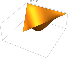
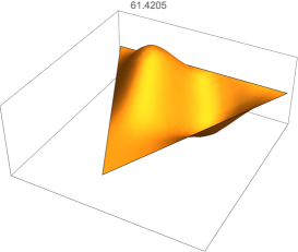
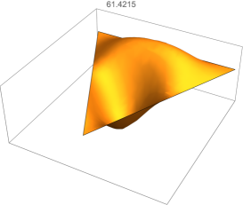
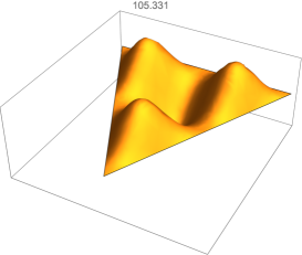
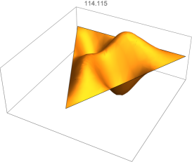
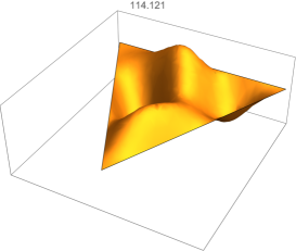
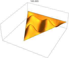
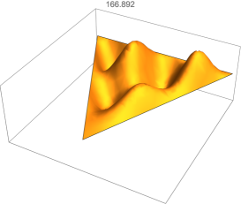
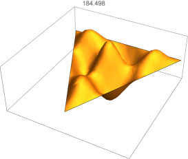
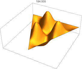
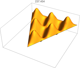
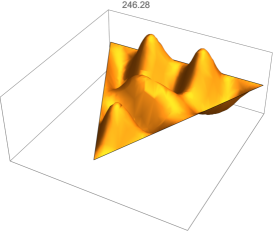
Figure 15: Twelve lowest eigenfunctions of the Laplacian on the equilateral triangle, used as our basis functions. The numbers on the top of each plot are their respective eigenvalues.

Appendix D Modified Jacobi coordinates for five-body systems

The tandard form of the Jacobi coordinates $\vec{r}_{i},i=1..5$ is

$$\vec{r}_{1} = \vec{x}_{1}-\vec{x}_{2},\,\,\,\vec{r}_{2}={1\over 2}\vec{x}_{1}+{1\over 2}\vec{x}_{2}-\vec{x}_{3},$$

$$\vec{r}_{3} = {1\over 3}\vec{x}_{1}+{1\over 3}\vec{x}_{2}+{1\over 3}\vec{x}_{3}-\vec{x}_{4},$$

$$\vec{r}_{4} = {1\over 4}\vec{x}_{1}+{1\over 4}\vec{x}_{2}+{1\over 4}\vec{x}_{3}+{1\over 4}\vec{x}_{4}-\vec{x}_{5},$$

$$\vec{r}_{5} = {1\over 5}(\vec{x}_{1}+\vec{x}_{2}+\vec{x}_{3}+\vec{x}_{4}+\vec{x}_{5})$$ (73)

with the determinant of this matrix – the Jacobian – being 1. The last coordinate $\vec{r}_{5}$ is the location of the center of mass, if those are coordinates, or 1/5 of the total momentum if $x_{i}$ are momentum fractions, and is in any case redundant.

As for two and three bodies, the simplest “star-like" potential simplifies to purely a diagonal form

$$\sum_{1}^{5}\vec{x}_{i}^{2}={1\over 2}\vec{r}_{1}^{2}+{2\over 3}\vec{r}_{2}^{2}+{3\over 4}\vec{r}_{3}^{2}+{4\over 5}\vec{r}_{4}^{2}+5\vec{r}_{5}^{2}$$ (74)

Further modification of the Jacobi coordinates is done by a simple rescaling of $\vec{r}_{i}$

$$\vec{r}_{1} \rightarrow \sqrt{2}\vec{\alpha},\,\vec{r}_{2}\rightarrow\sqrt{3/2}\vec{\beta},\,\vec{r}_{3}\rightarrow\sqrt{4/3}\vec{\gamma},$$

$$\vec{r}_{4} \rightarrow \sqrt{5/4}\vec{\delta},\vec{r}_{5}\rightarrow\sqrt{1/5}\vec{\sigma}$$ (75)

which makes the “star-like" potential a sum of squares of greek-letter coordinates.

Another important potential, the “Ansatz A", is half the sum of ten binary potentials. If it is assumed quadratic, it is proportional to the same sum of squares in terms of greek-letter coordinates

$$V_{A} = {1\over 2}\sum_{i>j}(\vec{x}_{i}-\vec{x}_{j})^{2}$$ (76)

$$= {5\over 2}\big{(}\vec{\alpha}^{2}+\vec{\beta}^{2}+\vec{\gamma}^{2}+\vec{\delta}^{2}\big{)}$$ (77)

except that the $\vec{\sigma}$ term is missing (which is unimportant as it is constant anyway).

In sum: in proper coordinates, the confining five-body potentials $V_{star}$ and $V_{A}$, can be reduced to the sum of greek-letter coordinates squared. In our approach to the quantization of $\vec{x}_{i}\rightarrow i\partial/\partial\vec{p}_{i}$, these operators take the form of Laplacians. The appropriate basis function are eigenfunctions of the Laplacian on the four-dimensional 5-simplex, the descendants of our basis on an equilateral triangle for three bodies.

Appendix E The coupling constant of instanton-induced ’t Hooft vertex

^′t Hooft standard interaction for two light flavors reads ${\bf q}=({\bf u},{\bf d})$

$${\cal L}_{qq}=2\bigg{(}\frac{\Delta M^{2}_{q}}{n}\bigg{)}\,\,\left({\rm det}\,\overline{\bf q}_{R}{\bf q}_{L}\,\,+\,\,{\rm det}\,\overline{\bf q}_{L}{\bf q}_{R}\right)$$ (78)

The light constituent quark mass, for the original parameters of the (dilute) random instanton liquid model (RILM) is Chernyshev et al. (1995); Kock et al. (2020)

$$\Delta M_{q}\sim\sqrt{\frac{n}{2N_{c}}}\bigg{(}\frac{4\pi^{2}\rho^{2}}{\Sigma_{0}}\bigg{)}\sim 420\,{\rm MeV}$$ (79)

with the zero mode integral

$$\Sigma_{0}=\bigg{(}\int\frac{d^{4}k}{(2\pi)^{4}}k^{2}\varphi^{\prime 4}_{I}(k)\bigg{)}^{\frac{1}{2}}\sim(240\,{\rm MeV})^{-1}$$

In singular gauge, the Fourier transform of the fermionic zero-mode profile is

$$\varphi_{I}^{\prime}(k)=\pi\rho^{2}\bigg{(}I_{0}(z)K_{0}(z)-I_{1}(z)K_{1}(z)\bigg{)}^{\prime}_{z=k\rho/2}$$ (81)

The prime is a z-derivative, and $I,K$ are modified Bessel functions. This function with the canonical value $\rho=1/3\,fm$, gives a dependence of the constituent quark mass on the virtuality $k$ in good agreement with phenomenology and lattice studies.

Note that (79) is not analytic in the packing fraction $n$, as expected from the spontaneous breaking of a symmetry Pobylitsa (1989). It differs slightly from the analytic coupling extracted from a naive random approximation, also used in our earlier analyses. More specifically, (79) gives

$$G_{tHooft}=2\bigg{(}\frac{\Delta M^{2}_{q}}{n}\bigg{)}\approx 35\,GeV^{-2}$$ (82)

which is to be compared to $17\,{\rm GeV}^{-2}$ using the naive approximation (see Eq. 62 in Shuryak and Zahed (2021a)).

Appendix F Sea production, to the first order in ’t Hooft vertex

The kinematics and the expression for the probability of the quark sea pair production has been given in (58). This relatively complicated expression need to be integrated over the 3-quark phase space, which is basically a 5-dimensional integral over $x,z,p_{\perp},k_{\perp}$ and the azimuthal angle between those two vectors.

The expression as written diverges at large momenta. If we would use the NJL model, the integrals should go to an arbitrary UV cutoff $\Lambda$. Fortunately, the instanton-induced coupling is naturally cutoff by the instanton size $\rho$. Its exact form is given by the Fourier transform of fermionic zero modes, which at large momenta asymptotes simply to $e^{-p\rho}$. Since both momentum integrals are basically $\int e^{-p\rho}p^{2}(dp/p)$, their main contribution is at the scale $p_{*}\approx 2/\rho\sim 1.2\,GeV$. So, the scale of this process is close to our assumed ^′unification scale^′ of 1 $GeV$.

Let us consider separately the domains in which $p>k$ and $p<k$, and expand in the $p/k$ (or $k/p$) ratio. It turns out that the large square bracket in (58) simplifies to

$${xz(1-x-z))\over(1-x)^{2}}+{\cal O}\bigg{(}\frac{k_{\perp}^{2}}{p_{\perp}^{2}}\bigg{)}$$

as the first order term $O(k_{\perp}/p_{\perp})$ vanishes by angle average. Therefore the $x,z$ integrals separate from the momentum integrals. The former one needs to be taken over the physical region, meaning that all three $x_{i}\in[0,1]$ and their divergencies are regulated by a small $\epsilon$. The result for the $p>k$ region is the same as for the $k>p$, and their total sum is

$$dN={G_{Hooft}^{2}\over 4}{1\over 16\pi^{4}\rho^{4}}\,{\rm log}({e^{2}\over 4\epsilon})$$ (83)

where the regulator $\epsilon$ corresponds to the minimal momentum fraction $\sim m_{q}/P$.

Appendix G Reduction of ’t Hooft interaction on the light front

To analyze the ’t Hooft determinantal interaction (78) on the light front, we use the free particle $u(p,s)$ and antiparticle $v(p,s)$ spinors, solutions to the Dirac equation

$$u(p,s) = \frac{1}{\sqrt{2p^{+}}}(\not{p}+m_{Q})\gamma^{+}\chi(s)$$

$$v(p,s) = \frac{1}{\sqrt{2p^{+}}}(\not{p}-m_{Q})\gamma^{+}\chi(-s)$$ (84)

with $\gamma^{+}=\gamma^{0}+\gamma^{3}$ in the chiral representation, and the particle spin up-down 4-spinors $\sigma_{z}\chi(\pm)=\pm\chi(\pm)$. The anti-particle spinor is tied to the particle spinor by $v(p,s)=iu(-p,-s)$, and its conjugate by $\bar{v}(p,s)=i\bar{u}(-p,-s)$.

To reduce (78) into a 2-body interaction, we formally factorize the isospin content, and specialize to the particle-anti-particle channel, with

$$(1-\tau_{1}\cdot\tau_{2})(\bar{u}_{R}u_{L}(1)\bar{v}_{R}v_{L}(2)+\bar{u}_{L}u_{R}(1)\bar{v}_{L}v_{R}(2))$$

for the instanton plus anti-instanton contribution. Using the light front spinors (G) in momentum space, we have for the particle entry

$$\bar{u}_{L}(p_{2},s_{2})u_{R}(p_{1},s_{1})=\begin{pmatrix}m_{Q}\sqrt{\frac{p_{1}^{+}}{p_{2}^{+}}}&0\\ \sqrt{\frac{p_{2}^{+}}{p_{1}^{+}}}p_{1R}-\sqrt{\frac{p_{1}^{+}}{p_{2}^{+}}}p_{2R}&m_{Q}\sqrt{\frac{p_{2}^{+}}{p_{1}^{+}}}\end{pmatrix}\rightarrow\begin{pmatrix}m_{Q}&0\\ q_{R}&m_{Q}\end{pmatrix}=m_{Q}{\bf 1}+\frac{1}{2}\sigma^{-}q_{R}$$ (86)

with the convention for the spin-entries

$$[s_{2}s_{1}]=\begin{pmatrix}++&+-\\ -+&--\end{pmatrix}$$

Similarly, for the anti-particle entry, we have

$$\bar{v}_{L}(p_{2},s_{2})v_{R}(p_{1},s_{1})=i^{2}\begin{pmatrix}m_{Q}\sqrt{\frac{p_{2}^{+}}{p_{1}^{+}}}&-\sqrt{\frac{p_{2}^{+}}{p_{1}^{+}}}p_{1R}+\sqrt{\frac{p_{1}^{+}}{p_{2}^{+}}}p_{2R}\\ 0&m_{Q}\sqrt{\frac{p_{1}^{+}}{p_{2}^{+}}}\end{pmatrix}\rightarrow\begin{pmatrix}-m_{Q}&q_{R}\\ 0&-m_{Q}\end{pmatrix}=-m_{Q}{\bf 1}+\frac{1}{2}\sigma^{+}q_{R}$$

with $q_{R}=p_{1R}-p_{2R}$, for a meson with net $P_{T}=0$. The rightmost equation follows from the eikonalization of the particle line with $p_{2}^{+}\approx p_{1}^{+}$ but $p_{\perp 2}\neq p_{\perp 1}$, as per our use of the straight Wilsonian lines in the general derivation of the potentials.

To move back to light front space, we use the inverse Fourier transform, which gives the local light front Hamiltonian (V.3) since

$$\int_{0}^{1}\frac{dx}{\pi}\frac{dk_{\perp}}{(2\pi)^{2}}e^{-ixP^{+}x^{-}-ik_{\perp}b_{\perp}}=\delta(P^{+}x^{-})\delta(b_{\perp})$$

The ultra-local and boost-invariant (G), is to be compared to

$$2M\delta(\xi_{x})\equiv 2M\delta(((\gamma x^{-})^{2}+b_{\perp}^{2})^{\frac{1}{2}})$$ (89)

with the Lorentz factor $\gamma=P^{+}/M$, which is also ultra-local and boost-invariant. The contribution $\gamma x^{-}$ reflects on the time dilatation effect on the light front. $\xi_{x}$ is the natural invariant distance, when the light front Hamiltonian is extracted from the Wilson lines, using the analytical construction discussed above and in our preceding studies Shuryak and Zahed (2021b, c, 2022).

Appendix H PDFs and formfactors in holography

The QCD gravity dual or holographic models are not used or discussed in this series of works. However, to put our results in perspective with those nonperturbative treatments of QCD in the double limit of large $N_{c}$ and strong ^′t Hooft coupling, we will briefly comment on some of their aspects in relation to LFWs and formfactors.

Formally, the holographic models provide a description of hadrons as modes of some bulk (5d) effective fields. The hadronic masses and wave functions $\psi_{n}(z)$ are defined from Schroedinger-like equations in the 5-th holographic coordinate $z$. “Holograms" obtained by certain prescriptions, project bulk wave functions to the boundary $z=0$. They yield distributions of certain quantities like e.g. the stress tensor $T^{\mu\nu}(x)$. While such a procedure does define certain hadronic sizes and shapes, there is no access to their internal substructure in terms of quarks/gluons.

Holography and pQCD have little in common, and their predictions do not agree in general. While the latter describes hard processes in the weak coupling regime, the former addresses QCD processes at strongly coupling and large $N_{c}$, in the semi-hard and soft regimes.

In holography, a struck quark with large momentum does not create a jet but rather a very wide flow of energy Lin and Shuryak (2008). In its evolution all the partons migrate to small $x$ Polchinski and Strassler (2002); Hatta et al. (2008), where the physics is well captured by open and closed string excitations (Pomerons and Reggeons).

Inelastic DIS or hard elastic scattering are well defined in holography Polchinski and Strassler (2002), with structure functions and formfactors. There is certain confusion in the literature about the relationship of these results to pQCD and partonic physics.

Holography and pQCD both have scattering rules for hard elastic processes, as originally noted in Polchinski and Strassler (2002). The hard elastic turn requires the involvement of the full hadron in the conformal limit, features that are shared by both holography and QCD. In pQCD, this follows from the fact that all the partons in a given hadron, have to undergo a “turn-around" under a hard scattering, which implies the probability $(1/Q^{2})^{n-1}$ with $n$ being the number of partonic constituents in the hadron Brodsky and Farrar (1973). In holography, a virtual photon has extension $1/Q$ in the holographic z-coordinate, and for a hard hit in bulk, the hadron has also to shrink to a size $1/Q^{\tau-1}$ with probability $P\sim(1/Q^{2})^{\tau-1}$. Here $\tau$ is the “bulk" dimension of the field describing a hadron (of the corresponding double trace 5d operators ). For the elastic processes, weak and strong coupling scaling laws are both known, and they are similar with $\tau$ identified as $n$ Polchinski and Strassler (2002).

In inelatic DIS processes, a virtual photon of size $1/Q$ scatters on a quark parton with probability 1 because it is pointlike. In contrast, a scattering off a hadron can only happen if it shrinks to the same size. The corresponding wave function is $(1/Q^{2})^{\tau-1}$. While $\tau$ is also sometimes called “anomalous dimention", it depends on the hadron field behavior in 5 dimensions, and has nothing to do with the “anomalous dimensions" of perturbative operators. Neither $\alpha_{s}(Q^{2})$ nor quarks or gluons are present in the bulk fields or actions. In DIS $s=Q^{2}(1/x-1)$ is constant. So the $F_{2}(x)$ structure function at large $Q^{2}$ and large $x\rightarrow 1$ are related. In fact one can write the structure function in the generic form

$$F_{2}(x,Q^{2})\sim Q^{2}\bigg{|}\bigg{(}\frac{1}{Q^{2}}\bigg{)}^{\tau-1}\bigg{|}^{2}\,\big{(}s=Q^{2}(1-x)\big{)}^{\alpha}$$

where $\alpha$ is $arbitrary$. To reproduce the hard scattering rule asymptotically, we $may$ set it to some value, e.g. $\alpha=\tau-2$,

$$F_{2}(x,Q^{2})\rightarrow\bigg{(}\frac{1}{Q^{2}}\bigg{)}^{\tau-1}\,(1-x)^{\tau-2}$$ (91)

to reproduce the holographic DIS result on a nucleon with a “reasonable" $\tau=3$, or for a meson with $\tau=2$ Polchinski and Strassler (2002). Yet there is still no Bjorken scaling at large $Q^{2}$!

Furthermore, the large $x$ behavior in (91) is different from that expected from the Drell-Yan-West scaling rule Drell and Yan (1970); West (1970). To reproduce it one would require $Q^{2}$ independence of the structure function (H) as per Bjorken scaling, which fixes another power of $\alpha=2\tau-3$ in (91). Indeed, this rule follows from the existence of the LFWFs in terms of constituents, which is absent in holography.

References

- Shuryak and Zahed (2021a) E. Shuryak and I. Zahed, (2021a), arXiv:2110.15927 [hep-ph] .
- Shuryak and Zahed (2021b) E. Shuryak and I. Zahed, (2021b), arXiv:2111.01775 [hep-ph] .
- Shuryak and Zahed (2021c) E. Shuryak and I. Zahed, (2021c), arXiv:2112.15586 [hep-ph] .
- Shuryak and Zahed (2022) E. Shuryak and I. Zahed, (2022), arXiv:2202.00167 [hep-ph] .
- Carroll et al. (1968) J. Carroll, D. B. Lichtenberg, and J. Franklin, Phys. Rev. 174, 1681 (1968).
- Jaffe and Wilczek (2003) R. L. Jaffe and F. Wilczek, Phys. Rev. Lett. 91, 232003 (2003), arXiv:hep-ph/0307341 .
- Barabanov et al. (2021) M. Y. Barabanov et al., Prog. Part. Nucl. Phys. 116, 103835 (2021), arXiv:2008.07630 [hep-ph] .
- Schäfer and Shuryak (1998) T. Schäfer and E. V. Shuryak, Rev. Mod. Phys. 70, 323 (1998), arXiv:hep-ph/9610451 .
- Schäfer et al. (1994) T. Schäfer, E. V. Shuryak, and J. J. M. Verbaarschot, Nucl. Phys. B 412, 143 (1994), arXiv:hep-ph/9306220 .
- Betman and Laperashvili (1985) R. G. Betman and L. V. Laperashvili, Yad. Fiz. 41, 463 (1985).
- Praschifka et al. (1989) J. Praschifka, R. T. Cahill, and C. D. Roberts, Int. J. Mod. Phys. A 4, 4929 (1989).
- Thorsson and Zahed (1990) V. Thorsson and I. Zahed, Phys. Rev. D 41, 3442 (1990).
- Rapp et al. (1998) R. Rapp, T. Schäfer, E. V. Shuryak, and M. Velkovsky, Phys. Rev. Lett. 81, 53 (1998), arXiv:hep-ph/9711396 .
- Alford et al. (1998) M. G. Alford, K. Rajagopal, and F. Wilczek, Phys. Lett. B 422, 247 (1998), arXiv:hep-ph/9711395 .
- Schäfer and Shuryak (2001) T. Schäfer and E. V. Shuryak, Lect. Notes Phys. 578, 203 (2001), arXiv:nucl-th/0010049 .
- Lu et al. (2021) Y. Lu, D. Binosi, M. Ding, C. D. Roberts, H.-Y. Xing, and C. Xu, Eur. Phys. J. A 57, 115 (2021), arXiv:2103.03960 [hep-ph] .
- Green et al. (2010) J. Green, J. Negele, M. Engelhardt, and P. Varilly, PoS LATTICE2010, 140 (2010), arXiv:1012.2353 [hep-lat] .
- Francis et al. (2022) A. Francis, P. de Forcrand, R. Lewis, and K. Maltman, Rev. Mex. Fis. Suppl. 3, 0308082 (2022), arXiv:2201.03332 [hep-lat] .
- Karliner and Rosner (2014) M. Karliner and J. L. Rosner, Phys. Rev. D 90, 094007 (2014), arXiv:1408.5877 [hep-ph] .
- Karliner and Rosner (2017) M. Karliner and J. L. Rosner, Phys. Rev. Lett. 119, 202001 (2017), arXiv:1707.07666 [hep-ph] .
- Jia and Vary (2019) S. Jia and J. P. Vary, Phys. Rev. C 99, 035206 (2019), arXiv:1811.08512 [nucl-th] .
- Shuryak and Zahed (2004) E. Shuryak and I. Zahed, Phys. Lett. B 589, 21 (2004), arXiv:hep-ph/0310270 .
- Brodsky et al. (2015) S. J. Brodsky, A. Deur, G. F. de Téramond, and H. G. Dosch, Int. J. Mod. Phys. Conf. Ser. 39, 1560081 (2015), arXiv:1510.01011 [hep-ph] .
- Chernyshev et al. (1995) S. Chernyshev, M. A. Nowak, and I. Zahed, Phys. Lett. B 350, 238 (1995), arXiv:hep-ph/9409207 .
- Shuryak (1982) E. V. Shuryak, Nucl. Phys. B 203, 140 (1982).
- Pobylitsa (1989) P. V. Pobylitsa, Phys. Lett. B 226, 387 (1989).
- Faccioli and Shuryak (2001) P. Faccioli and E. V. Shuryak, Phys. Rev. D 64, 114020 (2001), arXiv:hep-ph/0106019 .
- Shuryak (2019) E. Shuryak, Phys. Rev. D 100, 114018 (2019), arXiv:1908.10270 [hep-ph] .
- Drell and Yan (1970) S. D. Drell and T.-M. Yan, Phys. Rev. Lett. 24, 181 (1970).
- West (1970) G. B. West, Phys. Rev. Lett. 24, 1206 (1970).
- Lepage and Brodsky (1980) G. P. Lepage and S. J. Brodsky, Phys. Rev. D 22, 2157 (1980).
- Qattan and Arrington (2012) I. A. Qattan and J. Arrington, Phys. Rev. C 86, 065210 (2012), arXiv:1209.0683 [nucl-ex] .
- Brodsky and Farrar (1973) S. J. Brodsky and G. R. Farrar, Phys. Rev. Lett. 31, 1153 (1973).
- Shuryak and Zahed (2021d) E. Shuryak and I. Zahed, Phys. Rev. D 103, 054028 (2021d), arXiv:2008.06169 [hep-ph] .
- Hou et al. (2021) T.-J. Hou et al., Phys. Rev. D 103, 014013 (2021), arXiv:1912.10053 [hep-ph] .
- Kharzeev and Levin (2017) D. E. Kharzeev and E. M. Levin, Phys. Rev. D 95, 114008 (2017), arXiv:1702.03489 [hep-ph] .
- Dove et al. (2021) J. Dove et al. (SeaQuest), Nature 590, 561 (2021), [Erratum: Nature 604, E26 (2022)], arXiv:2103.04024 [hep-ph] .
- Dorokhov and Kochelev (1993) A. E. Dorokhov and N. I. Kochelev, Phys. Lett. B 304, 167 (1993).
- Towell et al. (2001) R. S. Towell et al. (NuSea), Phys. Rev. D 64, 052002 (2001), arXiv:hep-ex/0103030 .
- Basso et al. (2016) E. Basso, C. Bourrely, R. Pasechnik, and J. Soffer, Nucl. Phys. A 948, 63 (2016), arXiv:1509.07988 [hep-ph] .
- Alberg and Miller (2019) M. Alberg and G. A. Miller, Phys. Rev. C 100, 035205 (2019), arXiv:1712.05814 [nucl-th] .
- Alberg et al. (2022) M. Alberg, L. Ehinger, and G. A. Miller, Phys. Rev. D 105, 114054 (2022), arXiv:2108.12439 [nucl-th] .
- Eichten et al. (1992) E. J. Eichten, I. Hinchliffe, and C. Quigg, Phys. Rev. D 45, 2269 (1992).
- Rapp et al. (2000) R. Rapp, T. Schäfer, E. V. Shuryak, and M. Velkovsky, Annals Phys. 280, 35 (2000), arXiv:hep-ph/9904353 .
- Kock et al. (2020) A. Kock, Y. Liu, and I. Zahed, Phys. Rev. D 102, 014039 (2020), arXiv:2004.01595 [hep-ph] .
- Lin and Shuryak (2008) S. Lin and E. Shuryak, Phys. Rev. D 77, 085014 (2008), arXiv:0711.0736 [hep-th] .
- Polchinski and Strassler (2002) J. Polchinski and M. J. Strassler, Phys. Rev. Lett. 88, 031601 (2002), arXiv:hep-th/0109174 .
- Hatta et al. (2008) Y. Hatta, E. Iancu, and A. H. Mueller, JHEP 05, 037 (2008), arXiv:0803.2481 [hep-th] .