An automatic $L_{1}$-based regularization method for the analysis of FFC dispersion profiles with quadrupolar peaks

Abstract

Fast Field-Cycling Nuclear Magnetic Resonance relaxometry is a non-destructive technique to investigate molecular dynamics and structure of systems having a wide range of applications such as environment, biology, and food. Besides a considerable amount of literature about modeling and application of such technique in specific areas, an algorithmic approach to the related parameter identification problem is still lacking. We believe that a robust algorithmic approach will allow a unified treatment of different samples in several application areas. In this paper, we model the parameters identification problem as a constrained $L_{1}$-regularized non-linear least squares problem. Following the approach proposed in [Analytical Chemistry 2021 93 (24)], the non-linear least squares term imposes data consistency by decomposing the acquired relaxation profiles into relaxation contributions associated with ${{}^{1}H}-{{}^{1}H}$ and ${{}^{1}H}-{{}^{14}N}$ dipole-dipole interactions. The data fitting and the $L_{1}$-based regularization terms are balanced by the so-called regularization parameter.

For the parameters identification, we propose an algorithm that computes, at each iteration, both the regularization parameter and the model parameters. In particular, the regularization parameter value is updated according to a Balancing Principle and the model parameters values are obtained by solving the corresponding $L_{1}$-regularized non-linear least squares problem by means of the non-linear Gauss-Seidel method. We analyse the convergence properties of the proposed algorithm and run extensive testing on synthetic and real data. A Matlab software, implementing the presented algorithm, is available upon request to the authors.

[label1]organization=Department of Mathematics, University of Bologna, country=Italy

[label2]organization=Department of Biological, Chemical and Pharmaceutical Sciences and Technologies, University of Palermo, country=Italy

[label3]organization=Department of Agricultural, Food and Forest Sciences, University of Palermo, country=Italy

[label4]organization=Department of Civil, Chemical, Environmental, and Materials Engineering, University of Bologna, country=Italy

1 Introduction

Fast Field-Cycling (FFC) Nuclear Magnetic Resonance (NMR) relaxometry is a non-destructive magnetic resonance technique which is particularly useful in revealing information on slow molecular dynamics, which can only be carried out at very low magnetic field strengths. Standard NMR relaxation experiments are only performed in a relatively large fixed magnetic field that determines the resonance frequency of the molecules under investigation. Conversely, FFC-NMR relaxometry [1, 2] provides relaxation studies in a remarkably wide frequency range from approximately 1 kHz to 120 MHz. The FFC technique allows one to evaluate how the rate $R_{1}$ (also referred to as longitudinal relaxation rate) of a sample varies by changing the strength of an applied magnetic field, so forming the NMR Dispersion (NMRD) profiles. Therefore, FFC-NMR relaxometry measurements can detect the motion across a wide range of timescales (from millisecond to picoseconds) within an experiment. In addition, frequency-dependent relaxation studies have the exceptional potential to reveal the underlying mechanisms of molecular motion (not just its timescale). Spin relaxation theory represents relaxation rates as linear combinations of spectral density functions (Fourier transform of the time correlation function) characterising the motional frequencies and their intensities present in the correlation function [3]. However, complex spins dynamical interactions may occur such as the Quadrupole Relaxation Enhancement (QRE) due to their intramolecular magnetic dipolar coupling with quadrupole nuclei of arbitrary spins $S\geq 1$ [4, 5]. In the case of nitrogen-containing systems, for instance, the presence of QRE is represented by local maxima or peaks of the $R_{1}$ profiles due to ${}^{1}H-{{}^{14}N}$ interactions. The positions of the peaks depend on the quadrupole parameters which are determined by the electric field gradient tensor at the ${}^{14}N$ position. Consequently, even subtle changes in the electronic structure around ${}^{14}N$ reflect in changes of the position and shape of the quadrupole peaks. The QRE is a very sensitive fingerprint of molecular arrangement which has a wide range of applications ranging from environmental science [6], the study of ionic liquids, proteins [5] and food [7, 8].

Despite the consistent literature about the modeling of relaxation rate $R_{1}$ of protons fluids within a confined environment (see for instance [9, 10, 11]) and applications of FFC-NMR (see for example [12] and references therein), the study of a computational framework for the automatization of the FFC-NMR analysis is still missing. To the authors’ best knowledge, only P. Lo Meo et al. [13] propose a computational approach where, following the “model-free” approach introduced by [14, 15], the relaxation rate $R_{1}$ is represented as the sum of a constant term (offset) accounting for very “fast” molecular motion, a term describing proper ${}^{1}H-{{}^{1}H}$ relaxation as an integral function of the correlated time distribution function, and a non-linear term depending on several characteristic parameters related to the QRE occurence.

Therefore, the analysis of the NMRD profiles requires the solution of a parameter identification problem dealing with the estimation of the offset term, the correlation time distribution and the QRE parameters. In the present contribution, we formulate the parameter identification problem as a regularized non-linear least squares problem with box constraints and we propose a completely automatic strategy for its solution. In particular, the objective function contains a non-linear least squares term, imposing data consistency, and a $L_{1}$-based regularization term, accounting for the known sparsity of the correlation time distribution function. These terms are balanced by the so-called regularization parameter. Physical constraints on the unknown parameters lead to bound constraints in the optimization problem.

The parameter identification problem crucially depends on the regularization parameter whose value has to be properly identified in order to perform a meaningful NMRD analysis. Therefore, our mathematical model depends on several parameters: the NMRD parameters (i.e. the offset, the correlation time distribution), the QRE parameters, and the regularization parameter. The estimation of all these parameters is carried out by an iterative process where, at each iteration, the regularization parameter is computed according to a balancing principle [16]. The NMRD and QRE parameters are estimated solving the corresponding constrained optimization problem by the constrained two-blocks non-linear Gauss-Seidel (GS) method [17, 18], since the unknown NMRD and QRE parameters can be naturally partitioned into two blocks. In the GS method, the objective function is iteratively minimized with respect to the offset and the correlation time distribution while the QRE parameters are held fixed; then, fixed the updated values for the offset and the correlation time distribution, the objective is minimized with respect to the QRE parameters. The first subproblem involves solving a constrained linear least squares problem, obtained by the model-free approach [13], with an $L_{1}$ regularization term. The second subproblem requires the solution of a constrained non-linear least squares problem.

This computational approach, separating the contribution due to the offset and the relaxation distributions from the parameters of the quadrupolar relaxation, is able to provide a very accurate fit not only of the overall NMRD profile, but also of the local maxima due to the QRE.

Besides analysing the convergence of the proposed approach, we tested it on synthetic and real data aiming to illustrate the algorithm efficiency and its robustness to data noise.

The main contributions of the present paper can be summarized as follows.

• We formulate the problem of identifying the offset, the correlation time distribution and the QRE parameters from the NMRD profiles as a $L_{1}$-regularized non-linear least squares problem with box constraints related to physical properties of the parameters.

• We derive an automatic procedure, named AURORA (AUtomatic $L_{1}$-Regularized mOdel fRee Analysis) for the identification of all the parameters of mathematical model, i.e, the NMRD parameters (the offset term, the correlation time distribution), the QRE parameters and the regularization parameter and we analyse its convergence properties.

• We prove the robustness of the proposed approach to data noise by testing it on synthetic and real NMRD profiles.

The remainder of this paper is organised as follows. In section 2 we present the parameter identification problem; in section 3 we introduce the solution method, analyse its properties and present the AURORA algorithm. The results from several numerical experiments are reported and discussed in section 4. Finally, in section 5, we draw some conclusions.

2 The parameter identification problem

In the following, we first describe the continuous model for NMRD profiles, then we derive its discretization and, finally, we present the parameter identification problem.

2.1 The continuous model of NMRD profiles

Following the model-free approach, [13] proposes a model for the NMRD profiles $R_{1}$ made of three components:

$$R_{1}(\omega)=R_{0}+R^{HH}(\omega)+R^{NH}(\omega)$$ (1)

where $R_{0}$ is nonnegative offset keeping into account very fast molecular motions, the term $R^{HH}(\omega)$ describes the correlation distribution function $f(\tau)$ as:

$$R^{HH}(\omega)=\int_{0}^{\infty}\left[\frac{\tau}{(1+(\omega\tau)^{2})}+\frac{4\tau}{(1+4(\omega\tau)^{2})}\right]f(\tau)\ d\tau$$ (2)

where $\tau$ is the correlation time, i.e., the average time required by a molecule to rotate one radiant or to move for a distance as large as its radius of gyration. The term $R^{HN}(\omega)$ describes the occurrence of the quadrupolar peaks [12]:

$$R^{HN}(\omega)=C^{HN}\left(\begin{array}[]{ccc}\frac{1}{3}+\sin^{2}(\Theta)\cos^{2}(\Phi),&\frac{1}{3}+\sin^{2}(\Theta)\sin^{2}(\Phi),&\frac{1}{3}+\cos^{2}(\Theta)\\ \end{array}\right)\cdot\\ \left(\begin{array}[]{c}\displaystyle{\frac{\tau_{Q}}{1+(\omega-\omega_{-})^{2}\tau_{Q}^{2}}+\frac{\tau_{Q}}{1+(\omega+\omega_{-})^{2}\tau_{Q}^{2}}}\\ \displaystyle{\frac{\tau_{Q}}{1+(\omega-\omega_{+})^{2}\tau_{Q}^{2}}+\frac{\tau_{Q}}{1+(\omega+\omega_{+})^{2}\tau_{Q}^{2}}}\\ \displaystyle{\frac{\tau_{Q}}{1+(\omega-(\omega_{+}-\omega_{-}))^{2}\tau_{Q}^{2}}+\frac{\tau_{Q}}{1+(\omega+(\omega_{+}-\omega_{-}))^{2}\tau_{Q}^{2}}}\\ \end{array}\right)$$ (3)

where

• $C^{HN}$ refers to “the gyromagnetic ratios and the average interaction distance of the nuclei”;

• $\Theta$ and $\Phi$ are two angles accounting for “ the orientation of the ${}^{1}H-^{14}N$ dipole-dipole axis with respect to the principal axis system of the electric field gradient at the position of ${}^{14}N$ ”;

• $\tau_{Q}$ is the correlation time for the ${}^{1}H-{{}^{14}N}$ quadrupolar interaction;

• $\omega_{-}$ and $\omega_{+}$ are the angular frequency position of the peaks on the NMRD profiles.

(We remark that in (3) the $\cdot$ operator denotes the scalar product of two vectors.)

2.2 The discrete model for NMRD profiles

Before describing the discretization of the continuous model (1), let us introduce the following notation. Let $\boldsymbol{\omega}\in\mathbb{R}^{m}$ be the vector of the $m$ Larmor angular frequency values ($\omega=2\pi\nu$, $\nu$ in Mhz) at which $R_{1}$ is evaluated, and let ${\mathbf{y}}\in\mathbb{R}^{m}$ be the corresponding observations vector, i.e., $y_{i}=R_{1}(\omega_{i})$,  $i=1,\ldots,m$. Let ${\mathbf{f}}\in\mathbb{R}^{n}$ be the vector obtained by sampling $f(\tau)$ in $n$ logaritmically equispaced values $\tau_{1},\ldots,\tau_{n}$. Finally, let $\boldsymbol{\psi}\in\mathbb{R}^{6}$ be such that $\psi_{1}\equiv C^{HN}$ , $\psi_{2}\equiv\sin^{2}(\Theta)$, $\psi_{3}\equiv\sin^{2}(\Phi)$, $\psi_{4}\equiv\tau_{Q}$, $\psi_{5}\equiv\omega_{-}$, $\psi_{6}\equiv\omega_{+}$. The discrete model, obtained by discretizing the equations (2) and (3), is

$${\mathbf{y}}=\mathcal{F}({\mathbf{f}},\boldsymbol{\psi},R_{0})\equiv\mathcal{F}_{1}({\mathbf{f}})+\mathcal{F}_{2}(\boldsymbol{\psi})+R_{0}$$ (4)

where $\mathcal{F}:\mathbb{R}^{n+6+1}\rightarrow\mathbb{R}^{m}$. The first term $\mathcal{F}_{1}:\mathbb{R}^{n}\rightarrow\mathbb{R}^{m}$, only depending on ${\mathbf{f}}$, is a linear function of ${\mathbf{f}}$ deriving from the discretization of the integral for $R^{HH}$ in (2):

$$\mathcal{F}_{1}({\mathbf{f}})\equiv{\mathbf{K}}{\mathbf{f}},\ \hbox{with }{\mathbf{K}}\in\mathbb{R}^{m\times n},\ \ {\mathbf{f}}\in\mathbb{R}^{n}$$ (5)

and

$${\mathbf{K}}_{i,j}=\frac{\tau_{j}}{(1+(\omega_{i}\tau_{j})^{2})}+\frac{4\tau_{j}}{(1+4(\omega_{i}\tau_{j})^{2})},\quad i=1,\ldots,m,\;j=1,\ldots,n.$$

In a typical FFC-NMR experiment, $m\ll n$.

The second term $\mathcal{F}_{2}(\boldsymbol{\psi}):\mathbb{R}^{6}\rightarrow\mathbb{R}^{m}$ represents the quadrupolar component $R^{HN}$ (3) and only depends on the parameters $\psi_{j}$, $j=1,\ldots,6$:

$$\left(\mathcal{F}_{2}(\boldsymbol{\psi})\right)_{i}=\psi_{1}\left(\begin{array}[]{ccc}\frac{1}{3}+\psi_{2}(1-\psi_{3}),&\frac{1}{3}+\psi_{2}\cdot\psi_{3},&\frac{1}{3}+(1-\psi_{2})\\ \end{array}\right)\cdot\\ \left(\begin{array}[]{c}\displaystyle{\frac{\psi_{4}}{1+(\omega_{i}-\psi_{5})^{2}\psi_{4}^{2}}+\frac{\psi_{4}}{1+(\omega_{i}+\psi_{5})^{2}\psi_{4}^{2}}}\\ \displaystyle{\frac{\psi_{4}}{1+(\omega_{i}-\psi_{6})^{2}\psi_{4}^{2}}+\frac{\psi_{4}}{1+(\omega_{i}+\psi_{6})^{2}\psi_{4}^{2}}}\\ \displaystyle{\frac{\psi_{4}}{1+(\omega_{i}-(\psi_{6}-\psi_{5}))^{2}\psi_{4}^{2}}+\frac{\psi_{4}}{1+(\omega_{i}+(\psi_{6}-\psi_{5}))^{2}\psi_{4}^{2})}}\end{array}\right)$$ (6)

for $i=1,\ldots,m$.

The last term in $\mathcal{F}$ is the constant parameter $R_{0}\geq 0$ representing the offset in the NMRD curve.

2.3 The parameter identification problem

Mathematically, the problem of identifying the parameters ${\mathbf{f}}$, ${\boldsymbol{\psi}}$ and $R_{0}$ from the observations ${\mathbf{y}}$ is an ill-conditioned non linear inverse problem (4). In order to stabilize the parameter identification procedure, we use a regularization approach adding some a priori information on the unknown parameters. In particular, we use $L_{1}$ regularization to induce sparsity of ${\mathbf{f}}$ since the distribution $f(\tau)$ is known to be a sparse function with only a few non-null terms. Therefore, the parameter identification problem is reformulated as the following optimization problem

$$\begin{array}[]{ll}\min\limits_{{\mathbf{f}},\boldsymbol{\psi},R_{0}}&\displaystyle\|{\mathbf{y}}-(\mathcal{F}_{1}({\mathbf{f}})+\mathcal{F}_{2}(\boldsymbol{\psi})+R_{0})\|_{2}^{2}+\lambda\|{\mathbf{f}}\|_{1}\\ \text{s.t.}&{\mathbf{f}}\geq\mathbf{0},\\ &\boldsymbol{\psi}\in\mathcal{B}_{\psi},\\ &R_{0}\geq 0,\end{array}$$ (7)

where the set $\mathcal{B}_{\psi}$ defines the box constraints on ${\boldsymbol{\psi}}$:

$$\mathcal{B}_{\psi}=\big{\{}\boldsymbol{\psi}\,:\,\psi_{1}\in[0,\bar{C}];\ \psi_{2},\psi_{3}\in[0,1];\ \psi_{4}\in[0,\bar{\tau}];\ \psi_{5},\psi_{6}\in[\omega_{\ell},\omega_{u}]\big{\}}.$$ (8)

The bounds on the parameters $\psi_{i}$, $i=1,\ldots,6$, can be derived from the physical properties of the system and from the data ${\mathbf{y}}$; a deeper discussion on this topic will be given in the Section 4.

The regularization parameter $\lambda>0$ weights the contribution of the $L_{1}$ regularization term; the parameters $({\mathbf{f}},\boldsymbol{\psi},R_{0})$ obtained by solving (7) depend critically on the value of $\lambda$.

3 The solution method

The presented parameter identification method is an iterative procedure where, at each iteration, a value of the regularization parameter $\lambda$ is provided and the corresponding parameters $({\mathbf{f}}_{\lambda},\boldsymbol{\psi}_{\lambda},R_{0,_{\lambda}})$ are computed by solving problem (7). The constrained two-blocks non-linear Gauss-Seidel (GS) method [17, 18] is used for its solution. In the following, we firstly describe the GS method and recall its convergence properties, then we introduce the iterative procedure for the regularization parameter computation, and, finally, we draw the overall parameter identification procedure.

3.1 The constrained two-blocks Gauss-Seidel method

In this subsection, we describe the GS method used for the solution of the constrained optimization problem (7) for a fixed value of the regularization parameter $\lambda$. To this end, we partition the unknowns of (7) into two blocks such that the data fitting term is linear with respect to the first block and non-linear with respect to the second block. Therefore, we reformulate problem (7) as follows:

$$\begin{array}[]{ll}\min\limits_{{\mathbf{x}}_{1},{\mathbf{x}}_{2}}&\displaystyle g({\mathbf{x}}_{1},{\mathbf{x}}_{2})=\|{\mathbf{y}}-{\mathbf{K}}_{e}{\mathbf{x}}_{1}-\mathcal{F}_{2}({\mathbf{x}}_{2})\|_{2}^{2}+\lambda\|{\mathbf{x}}_{1}\|_{1}+\eta\|{\mathbf{x}}_{1}\|^{2}_{2}\\ \text{s.t.}&{\mathbf{x}}_{1}\in X_{1},\\ &{\mathbf{x}}_{2}\in X_{2},\end{array}$$ (9)

where

$${\mathbf{x}}_{1}\equiv({\mathbf{f}},R_{0}),\quad{\mathbf{x}}_{2}\equiv\boldsymbol{\psi}$$ (10)

$$X_{1}=\{{\mathbf{x}}_{1}\geq\mathbf{0}\},\quad X_{2}\equiv\mathcal{B}_{\psi}$$ (11)

and

$$\ {\mathbf{K}}_{e}=\left[\begin{array}[]{c c}{\mathbf{K}}&\mathbf{1}\end{array}\right]\in\mathbb{R}^{m\times(n+1)}.$$ (12)

The last $L_{2}$-based penalty term $\eta\|{\mathbf{x}}_{1}\|^{2}_{2}$ in the objective function has been introduced to ensure that ${\mathbf{K}}_{e}^{T}{\mathbf{K}}_{e}+\eta\mathbf{I}$ is a definite positive matrix; to this and, a small value for $\eta$, as $\eta=10^{-10}$ for example, can be fixed. Moreover, observe that in (9), the parameter $R_{0}$ has been included in the $L_{1}$-based penalty term.

The closed subsets $X_{1}\subseteq\mathbb{R}^{n+1}$ and $X_{2}\subseteq\mathbb{R}^{6}$ are both convex; the objective function $g({\mathbf{x}}_{1},{\mathbf{x}}_{2})$ is continuous and it is convex with respect to ${\mathbf{x}}_{1}$ for fixed ${\mathbf{x}}_{2}$, but it is not convex with respect to ${\mathbf{x}}_{2}$ for fixed ${\mathbf{x}}_{1}$. However, since ${\mathbf{K}}_{e}^{T}{\mathbf{K}}_{e}+\eta\mathbf{I}$ is definite positive and $X_{2}$ is bounded, it is easy to show that $g$ is coercive on $X_{1}\times X_{2}$.

Definition 3.1.

A function $g:\mathbb{R}^{q}\rightarrow\mathbb{R}$ is called coercive in $X$ if, for every sequence $\{{\mathbf{x}}^{(k)}\}\in X$ such that $\|{\mathbf{x}}^{(k)}\|\rightarrow\infty$, we have

$$\lim_{k\rightarrow\infty}g({\mathbf{x}}^{(k)})=+\infty$$

Proposition 3.1.

The function $g:\mathbb{R}^{n+1+6}\rightarrow\mathbb{R}$ such that

$$g({\mathbf{x}}_{1},{\mathbf{x}}_{2})=\|{\mathbf{y}}-{\mathbf{K}}_{e}{\mathbf{x}}_{1}-\mathcal{F}_{2}({\mathbf{x}}_{2})\|_{2}^{2}+\lambda\|{\mathbf{x}}_{1}\|_{1}+\eta\|{\mathbf{x}}_{1}\|^{2}_{2}$$

is coercive in $X_{1}\times X_{2}$.

Proof.

The function $g$ can be rewritten as

$$g({\mathbf{x}}_{1},{\mathbf{x}}_{2})={\mathbf{x}}_{1}^{T}({\mathbf{K}}_{e}^{T}{\mathbf{K}}_{e}+\eta\mathbf{I}){\mathbf{x}}_{1}+2{\mathbf{x}}_{1}^{T}{\mathbf{K}}_{e}^{T}(\mathcal{F}_{2}({\mathbf{x}}_{2})-{\mathbf{y}})+\|\mathcal{F}_{2}({\mathbf{x}}_{2})-{\mathbf{y}}\|^{2}+\lambda\|{\mathbf{x}}_{1}\|_{1}$$

where ${\mathbf{K}}_{e}^{T}{\mathbf{K}}_{e}+\eta\mathbf{I}$ is positive definite. Let $\{({\mathbf{x}}_{1}^{(k)},{\mathbf{x}}_{2}^{(k)})\}$ be a sequence in $X_{1}\times X_{2}$ such that $\lim_{k\rightarrow\infty}\|({\mathbf{x}}_{1}^{(k)},{\mathbf{x}}_{2}^{(k)})\|=\infty.$ Since $X_{2}$ is bounded, we have

$$\lim_{k\rightarrow\infty}\|{\mathbf{x}}_{1}^{(k)}\|=\infty\quad\text{and}\quad\lim_{k\rightarrow\infty}\|{\mathbf{x}}_{2}^{(k)}\|<\infty.$$ (13)

Let $\mu>0$ be the smallest eigenvalue of ${\mathbf{K}}_{e}^{T}{\mathbf{K}}_{e}+\eta\mathbf{I}$. It holds

$$g({\mathbf{x}}_{1}^{(k)},{\mathbf{x}}_{2}^{(k)}) \geq\mu\|{\mathbf{x}}_{1}^{(k)}\|^{2}-2\|{\mathbf{K}}_{e}^{T}(\mathcal{F}_{2}({\mathbf{x}}_{2}^{(k)})-{\mathbf{y}})\|\|{\mathbf{x}}_{1}^{(k)}\|+\lambda\|{\mathbf{x}}_{1}^{(k)}\|+$$

$$\quad+\|{\mathbf{K}}_{e}^{T}(\mathcal{F}_{2}({\mathbf{x}}_{2}^{(k)})-{\mathbf{y}})\|^{2}$$

$$\geq\left(\mu\|{\mathbf{x}}_{1}^{(k)}\|-2\|{\mathbf{K}}_{e}^{T}(\mathcal{F}_{2}({\mathbf{x}}_{2}^{(k)})-{\mathbf{y}})\|+\lambda\right)\|{\mathbf{x}}_{1}^{(k)}\|$$

From (13) we have $\mu\|{\mathbf{x}}_{1}^{(k)}\|-2\|{\mathbf{K}}_{e}^{T}(\mathcal{F}_{2}({\mathbf{x}}_{2}^{(k)})-{\mathbf{y}})\|+\lambda>0$ for sufficiently large $k$, then

$$\lim_{k\rightarrow\infty}g({\mathbf{x}}_{1}^{(k)},{\mathbf{x}}_{2}^{(k)})=+\infty$$

∎

Continuity and coerciveness ensure the existence of at least one global minimizer of $g({\mathbf{x}}_{1},{\mathbf{x}}_{2})$ in $X_{1}\times X_{2}$ [19].

In the constrained two-blocks Gauss-Seidel method, at each iteration, the objective function is minimized with respect to each of the block coordinate vectors ${\mathbf{x}}_{i}$ over the subsets $X_{i}$, $i=1,2$, as summarized in Algorithm 1, where the convergence condition is:

$$|g({\mathbf{x}}_{1}^{(k)},{\mathbf{x}}_{2}^{(k)})-g({\mathbf{x}}_{1}^{(k-1)},{\mathbf{x}}_{2}^{(k-1)})|\leq Tol_{GS}|g({\mathbf{x}}_{1}^{(k)},{\mathbf{x}}_{2}^{(k)})|.$$ (14)

Algorithm 1 Constrained two-blocks non-linear Gauss-Seidel method

1:function GS(${\mathbf{x}}_{1}^{(0)},{\mathbf{x}}_{2}^{(0)}$)

2:     Set $k=0$ and ${\mathbf{x}}^{(0)}=({\mathbf{x}}_{1}^{(0)},{\mathbf{x}}_{2}^{(0)})$.

3:     repeat

4:         $k=k+1$

5:         Set ${\mathbf{x}}_{1}^{(k)}\in\arg\min\limits_{{\mathbf{z}}\in X_{1}}\;g({\mathbf{z}},{\mathbf{x}}_{2}^{(k-1)})$

6:         Set ${\mathbf{x}}_{2}^{(k)}\in\arg\min\limits_{{\mathbf{z}}\in X_{2}}\;g({\mathbf{x}}_{1}^{(k)},{\mathbf{z}})$

7:     until convergence condition (14)

8:     return $({\mathbf{x}}_{1}^{(k)},{\mathbf{x}}_{2}^{(k)})$

9:end function

We observe that the GS method is well defined since each subproblem has solutions. Indeed, the function $g$ is strictly convex with respect of ${\mathbf{x}}_{1}$ and hence there exist at most one global minimum of $f$ over $X_{1}$ for fixed ${\mathbf{x}}_{2}$. On the other hand, Weierstrass’s theorem guarantees the existence of at least one global minimum of $g$ over $X_{2}$ for fixed ${\mathbf{x}}_{1}$ since $g$ is continuous and $X_{2}$ is a closed and bounded set.

For general nonconvex, constrained problems, convergence of sequences generated by the GS method to critical points has been proved in [18]. For the reader’s convenience, we report here the main convergence result for the GS method and we refer to [18] for its proof.

Theorem 3.2.

Consider the problem

$$\begin{array}[]{ll}\min\limits_{{\mathbf{x}}_{1},{\mathbf{x}}_{2}}&\displaystyle g({\mathbf{x}}_{1},{\mathbf{x}}_{2})\\ \text{s.t.}&{\mathbf{x}}_{1}\in X_{1},\\ &{\mathbf{x}}_{2}\in X_{2},\end{array}$$ (15)

where $g$ is a continuously differentiable function and the subsets $X_{i}$ are closed, nonempty and convex for $i=1,2$. Suppose that the sequence $\{({\mathbf{x}}_{1}^{(k)},{\mathbf{x}}_{2}^{(k)})\}$ generated by the two-blocks GS method has limit points. Then, every limit point of $\{({\mathbf{x}}_{1}^{(k)},{\mathbf{x}}_{2}^{(k)})\}$ is a critical point of the problem.

We have already observed that the objective function $g$ of (9) is coercive; since the level sets of continuous coercive functions are compact, the sequence $\{({\mathbf{x}}_{1}^{(k)},{\mathbf{x}}_{2}^{(k)})\}$ generated by the GS method has limit points (eventually, it has a convergent subsequence); hence, the GS method converges to critical points of (9).

We conclude this subsection with a remark on the solution of the two constrained subproblems to be solved at each iteration of algorithm 1. The first subproblem at step 3 is a $L_{1}$-regularized least squares problem with nonnegativity constraints:

$$\begin{array}[]{ll}\min\limits_{{\mathbf{z}}}&\displaystyle\|{\mathbf{w}}-{\mathbf{K}}_{e}{\mathbf{z}}\|_{2}^{2}+\lambda\sum_{i=1}^{m+1}z_{i}\\ \text{s.t.}&z_{i}\geq 0,\quad i=1,\ldots,m+1\end{array}$$ (16)

where ${\mathbf{w}}={\mathbf{y}}-\mathcal{F}_{2}({\mathbf{x}}_{2}^{(k)})$. For its solution, we use the truncated Newton interior-point method described in [20].

The second subproblem at step 4 is a bound constrained non-linear least squares problem:

$$\begin{array}[]{ll}\min\limits_{{\mathbf{z}}}&\displaystyle\|\mathcal{F}_{2}(\boldsymbol{{\mathbf{z}}})-{\mathbf{w}}\|^{2}\\ \text{s.t.}&{\mathbf{z}}\in X_{2}\end{array}$$ (17)

where ${\mathbf{w}}={\mathbf{K}}_{e}{\mathbf{x}}_{1}^{(k+1)}-{\mathbf{y}}$. For its solution, we use the Newton Projection method [21, 22] where the Hessian matrix is approximated as in the Levenberg-Marquardt method [23] since the Jacobian of $\mathcal{F}_{2}$ is ill-conditioned.

3.2 Computation of the regularization parameter $\lambda$

In order to correctly analyse the NMRD profiles, it is necessary to choose an appropriate value for the regularization parameter $\lambda$. Even if several parameter selection rules have been proposed in the literature for $L_{2}$-regularized minimization problems (see [24, 25, 26] for a theoretical discussion of such rules), the case of $L_{1}$-based regularization still remains largely unexplored. In [27, 28], the discrepancy principle has been investigated for nonsmooth regularization. This principle is difficult to be realized since it requires the prior knowledge of the noise norm and a solution of the discrepancy equation is not guaranteed to exist. In [16], the Balancing Principle (BP) has been proposed where the regularization parameter is selected by balancing, up to a multiplicative factor $\gamma$, the data fidelity and the regularization term, i.e,:

$$\gamma\lambda\|{\mathbf{x}}_{1}\|_{1}=\|{\mathbf{y}}-{\mathbf{K}}_{e}{\mathbf{x}}_{1}-\mathcal{F}_{2}({\mathbf{x}}_{2})\|_{2}^{2}+\eta\|{\mathbf{x}}_{1}\|^{2}_{2}$$ (18)

The regularization properties of the BP has been deeply investigated and a convergent fixed-point iterative scheme for its realization has been proposed in [16]. We set $\gamma=1$ which gives the following rule for the regularization parameter selection:

$$\lambda=\displaystyle\frac{\|{\mathbf{y}}-{\mathbf{K}}_{e}{\mathbf{x}}_{1}-\mathcal{F}_{2}({\mathbf{x}}_{2})\|_{2}^{2}+\eta\|{\mathbf{x}}_{1}\|^{2}_{2}}{\|{\mathbf{x}}_{1}\|_{1}}.$$

3.3 The parameter identification method

The proposed iterative method for the identification of both the NMRD parameters ${\mathbf{f}}$, ${\boldsymbol{\psi}}$ and $R_{0}$ and the regularization parameter $\lambda$ is outlined in algorithm 2 where, given an initial guess for $\lambda$, at each iteration, the NMRD parameters are computed by solving problem (7) by the GS method, and the regularization parameter value is updated by the BP until the following convergence condition is met:

$$|\lambda^{(k+1)}-\lambda^{(k)}|\leq Tol_{\lambda}|\lambda^{(k)}|,\ \ Tol_{\lambda}>0.$$ (19)

We refer to this method as AURORA (AUtomatic $L_{1}$-Regularized mOdel fRee Analysis).

Algorithm 2 AURORA 

1:Set $k=0$, $\eta=10^{-10}$ and choose a starting guess $\lambda^{(0)}$.

2:repeat

3:     $k=k+1$

4:     NMRD and QRE parameters update

$$\hbox{By algorithm \ref{alg:GS} compute }({\mathbf{x}}_{2}^{(k)},{\mathbf{x}}_{2}^{(k)})=GS({\mathbf{x}}_{1}^{(k-1)},{\mathbf{x}}_{2}^{(k-1)})\ \hbox{i.e.}$$

$$({\mathbf{x}}_{1}^{(k)},{\mathbf{x}}_{2}^{(k)})\in\arg\min\limits_{\begin{subarray}{c}{\mathbf{x}}_{1}\in X_{1}\\ {\mathbf{x}}_{2}\in X_{2}\end{subarray}}\displaystyle\;\|{\mathbf{y}}-{\mathbf{K}}_{e}{\mathbf{x}}_{1}-\mathcal{F}_{2}({\mathbf{x}}_{2})\|_{2}^{2}+\lambda^{(k)}\|{\mathbf{x}}_{1}\|_{1}+\eta\|{\mathbf{x}}_{2}\|^{2}_{2}$$

5:     Regularization parameter update

$$\lambda^{(k+1)}=\frac{\|{\mathbf{y}}-{\mathbf{K}}_{e}{\mathbf{x}}_{1}^{(k)}-\mathcal{F}_{2}({\mathbf{x}}_{2}^{(k)})\|_{2}^{2}+\eta\|{\mathbf{x}}_{2}^{(k)}\|^{2}_{2}}{\|{\mathbf{x}}_{1}^{(k)}\|_{1}}$$

6:until convergence condition (19)

7:return $({\mathbf{f}},R_{0})={\mathbf{x}}_{1}^{(k)}$ and ${\boldsymbol{\psi}}={\mathbf{x}}_{2}^{(k)}$ $\triangleright$ Result $({\mathbf{f}},R_{0},{\boldsymbol{\psi}})$

Following the analysis of the BP performed in [16], algorithm AURORA can be viewed as a fixed point-like scheme for the problem

$$\begin{array}[]{l}({\mathbf{x}}_{1}^{*},{\mathbf{x}}_{2}^{*})=\text{arg}\min\limits_{\begin{subarray}{c}{\mathbf{x}}_{1}\in X_{1}\\ {\mathbf{x}}_{2}\in X_{2}\end{subarray}}\ \|{\mathbf{y}}-{\mathbf{K}}_{e}{\mathbf{x}}_{1}-\mathcal{F}_{2}({\mathbf{x}}_{2})\|_{2}^{2}+\lambda^{*}\|{\mathbf{x}}_{1}\|_{1}+\eta\|{\mathbf{x}}_{1}\|^{2}_{2},\\ \lambda^{*}=\displaystyle\frac{\|{\mathbf{y}}-{\mathbf{K}}_{e}{\mathbf{x}}_{1}^{*}-\mathcal{F}_{2}({\mathbf{x}}_{2}^{*})\|_{2}^{2}+\eta\|{\mathbf{x}}_{1}^{*}\|^{2}_{2}}{\|{\mathbf{x}}_{1}^{*}\|_{1}}.\end{array}$$ (20)

The monotone convergence of the sequence $\{\lambda^{(k)}\}$ generated by the fixed point scheme has been proved in [16] when $\lambda^{(0)}$ is chosen in an interval containing only one solution of equation (18).

4 Results and Discussion

In this section, we present and discuss the results obtained by a set of numerical experiments to assess the accuracy, robustness and efficiency of the proposed algorithm. In paragraph 4.1, we describe the experimental setting. In paragraph 4.2, we test AURORA on a synthetic NMRD profile $R_{1}$ computed by the model (1) with assigned values of the parameters $\boldsymbol{\psi}$, ${\mathbf{f}}$ and $R_{0}$. We evaluate computational efficiency and accuracy of AURORA comparing it with some algorithms available in the Matlab optimization Toolbox. Moreover, we investigate the algorithm robustness in presence of data noise.
Then, in paragraph 4.3, we report the results of the analysis of NMRD profiles from two different samples: Dry Nanosponge (DN) and Parmigiano-Reggiano (PR) cheese.

4.1 Numerical Experimental setting

All numerical computations are carried out using Matlab R2021b on a laptop equipped with $2.9$ GHz Intel Core i7 quad-core processor and $16$ GB $2133$ MHz RAM.
For all tests, the values $\bar{C}$ and $\bar{\tau}$ in the constraints set $\mathcal{B}_{\psi}$ (8) are set equal to a value large enough so that the intermediate solutions $\psi_{1}^{(k)}$ and $\psi_{4}^{(k)}$ never reach such bounds. In our tests $\bar{C}=\bar{\tau}=100$ are suitable values. The interval $[\omega_{\ell},\omega_{u}]$ in (8), representing the region where $R_{1}$ interrupts its decaying behaviour due to QRE, is defined by inspection of the NMRD profile.
The starting guess for the parameter $\psi_{1}^{(0)}\equiv C^{HN}$ is obtained by the literature [5]:

$$C^{HN}=\frac{2}{3}\left(\frac{\mu_{0}}{4\pi}\frac{\gamma_{H}\gamma_{N}\hbar}{r_{NH}^{3}}\right)^{2}\approx 0.18\ \left[\frac{\mu s}{s^{2}}\right]$$ (21)

where the value of the physical constants is reported in table 1.

Constant	Description	Value
$\mu_{0}$	permeability of vacuum	$10^{-7}\ T^{2}J^{-1}m^{3}$
$\gamma_{H}$	${}^{1}H$ gyromagnetic factor	$2.577\ 10^{6}\ T^{-1}s^{-1}$
$\gamma_{N}$	${}^{14}N$ gyromagnetic factor	$3.078\ 10^{6}\ T^{-1}s^{-1}$
$\hbar$	reduced Planck’s constant	$1.05472\ 10^{-34}\ J\ s$
$r_{HN}$	${}^{1}H-^{14}N$ inter-spin distance	$1.4\ 10^{-10}\ m$

Table 1: Characteristic constants for $C^{HN}$ in (21).

Concerning the quadrupolar parameters, $\psi^{(0)}_{2}\equiv\sin^{2}{\Theta^{(0)}}$, $\psi^{(0)}_{3}\equiv\sin^{2}{\Phi^{(0)}}$, the initial values are equal to the mean of the corresponding upper and lower bounds in $\mathcal{B}_{\psi}$, i.e. $1/2$. The initial value of $\psi_{4}^{(0)}\equiv\tau_{Q}$, is set to $1$, while $\psi^{(0)}_{5}\equiv\omega_{-}^{(0)}$, and $\psi^{(0)}_{6}\equiv\omega_{+}^{(0)}$ are defined as follows:

$$\psi^{(0)}_{5}=\omega_{\ell}+\frac{1}{4}|\omega_{u}-\omega_{\ell}|,\ \ \ \psi^{(0)}_{6}=\omega_{u}-\frac{1}{4}|\omega_{u}-\omega_{\ell}|.$$

The computed results are evaluated by the Mean Squared Error (MSE)

$$\text{MSE}=\frac{\|R_{1}-\mathcal{F}({\mathbf{f}},\boldsymbol{\psi},R_{0})\|^{2}}{m},\ \$$

and the Parameter Relative Error (PRE):

$$\text{PRE}(x)=\frac{\|x^{exact}-x^{computed}\|^{2}}{\|x^{exact}\|^{2}}$$ (22)

with $x$ representing either the vector ${\mathbf{f}}$ or the scalars $R_{0}$, $\psi_{i}$, $i=1,\ldots,6$.
The components of the vector $\boldsymbol{\psi}$ are referenced by the name in the physical model (3), according to the mapping introduced in section 2.2, and reported in table (2) for convenience.

$C^{HN}$	$\Phi$	$\Theta$	$\tau_{Q}$	$\omega_{-}$	$\omega_{+}$
$\psi_{1}$	$asin(\sqrt{\psi_{2}})$	$asin(\sqrt{\psi_{3})})$	$\psi_{4}$	$\psi_{5}$	$\psi_{6}$

Table 2: Quadrupolar parameters mapping.

All the tests apply algorithm 2 with $Tol_{\lambda}=10^{-2}$ in (19) and algorithm 1 with $Tol_{GS}=10^{-6}$ in (14).
The computational cost is evaluated in terms of number of execution time.

4.2 Synthetic test Problem

To investigate the properties of AURORA, we first test it on the synthetic NMRD profile $R_{1}$ represented in figure 1(a), and obtained by setting the parameters of model (1) as in the second column of table 3, with the distribution function ${\mathbf{f}}^{*}$ represented in red in figure 2(a). Throughout the paragraph we use the frequencies $\nu$ instead of the angular frequencies $\omega$, i.e. $\nu_{-}\equiv\omega_{-}/(2\pi)$ and $\nu_{+}\equiv\omega_{+}/(2\pi)$.

	reference	computed	PRE
$R_{0}$	$3.69$	$3.6868$	$7.0267\ 10^{-4}$
$C^{HN}$	$18.84$	$18.8453$	$6.1449\ 10^{-5}$
$\tau_{Q}$	$0.96$	$0.9554$	$8.5033\ 10^{-6}$
$\Theta$	$1.09$	$1.0901$	$6.1449\ 10^{-5}$
$\Phi$	$0.57$	$0.5696$	$6.9199\ 10^{-4}$
$\nu_{-}$	$2.15$	$2.1502$	$5.7363\ 10^{-6}$
$\nu_{+}$	$2.87$	$2.8696$	$1.1316\ 10^{-6}$

Table 3: Model parameters: reference (second column), AURORA computed values (third column) and PRE (fourth column).

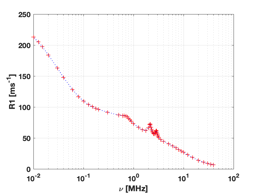
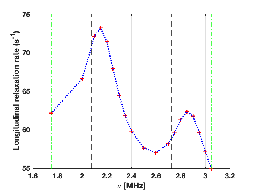
Figure 1: Synthetic sample. (a) Full NMRD profile (b) Zoom of NMRD profile in the reference interval $[\nu_{\ell},\nu_{u}]$ represented by the left and right green vertical lines. Left and right black vertical lines represent the values $\psi^{(0)}_{5}/(2\pi)$, $\psi^{(0)}_{6}/(2\pi)$ respectively.

The accuracy of the computed results can be appreciated in the correlation distribution ${\mathbf{f}}$ and $R_{1}$ curves shown in figure 2.

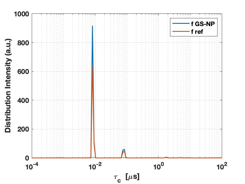
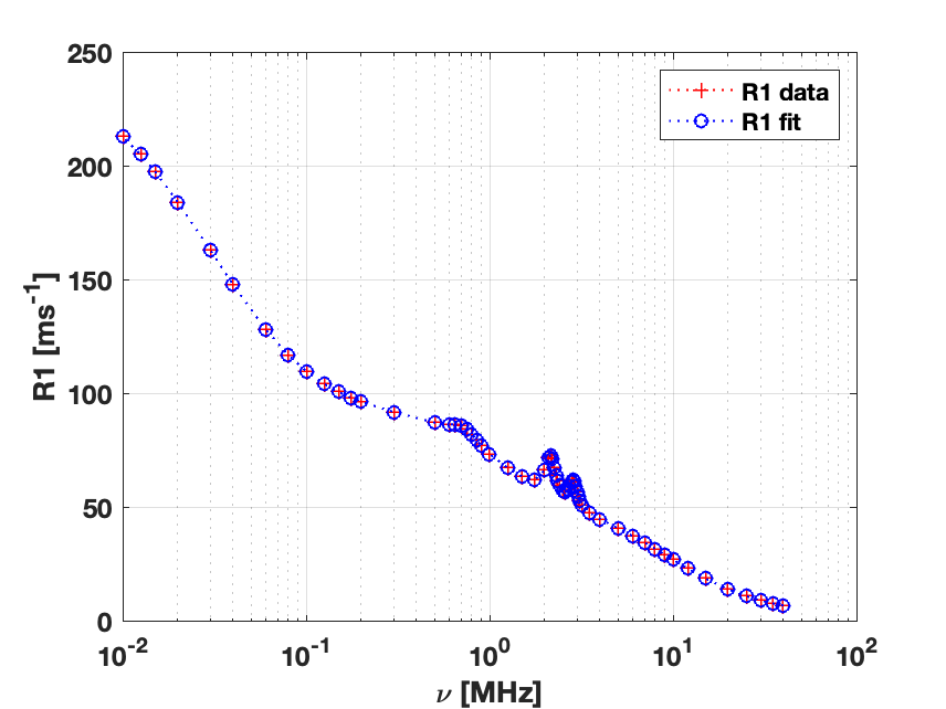
Figure 2: Synthetic sample. (a) Reference (red) and computed correlation distribution (blue). (b) Reference and computed $R_{1}$ profiles.

To test the convergence behaviour we evaluate the PRE and MSE at each step of the GS method in algorithm 1. Figure 3(a) shows the the behaviour of the relative errors for each parameter $({\mathbf{f}},R_{0},C^{HN},\Phi,\Theta,\tau_{Q},\nu_{-},\nu_{+})$ compared to their reference values. The convergence to reference parameters values is initially non monotonic for most parameters with the exception of $\tau_{Q}$ and $\nu_{-}$. On the contrary, MSE has monotonic decrease as reported in figure 3(b).

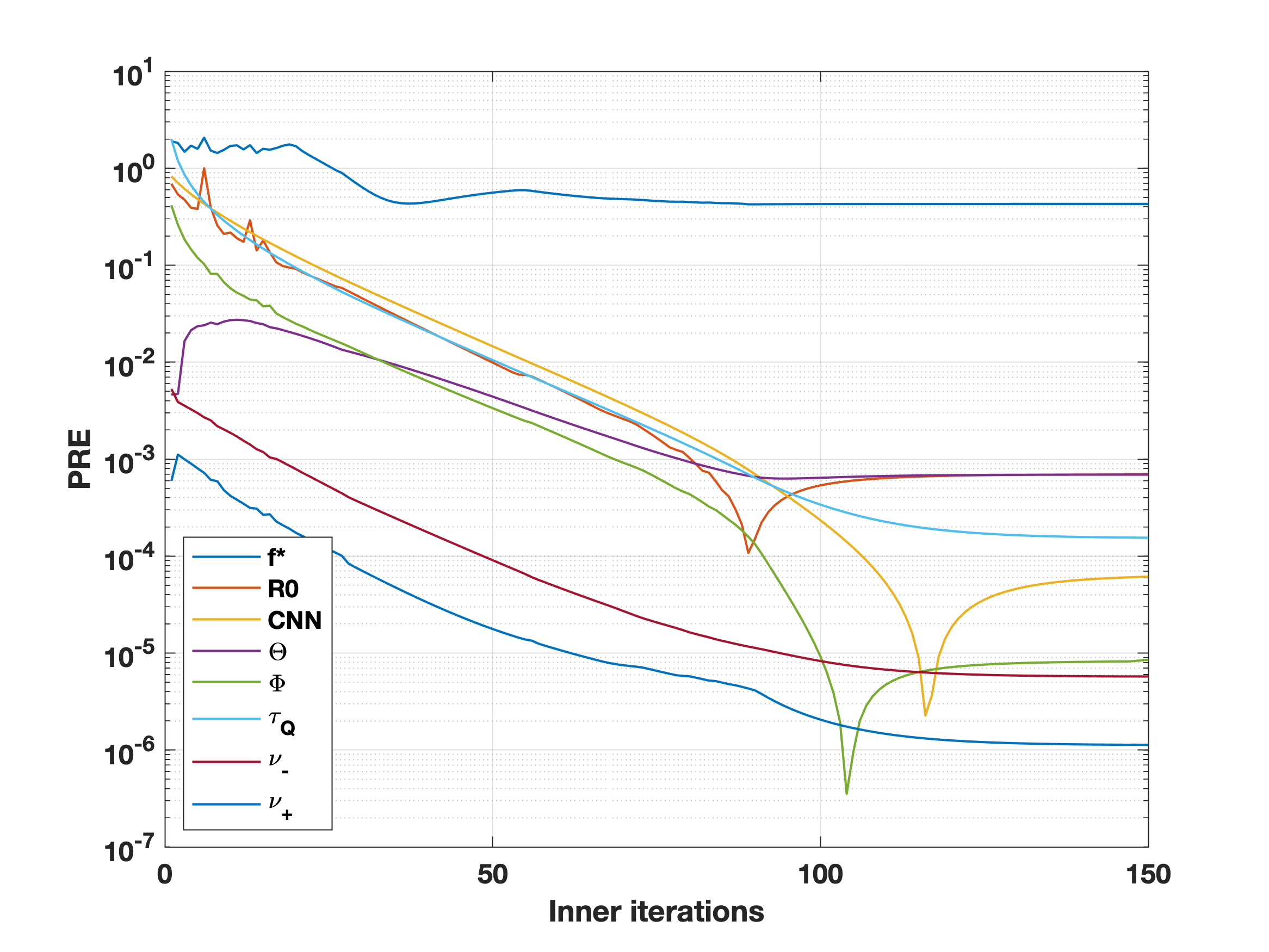
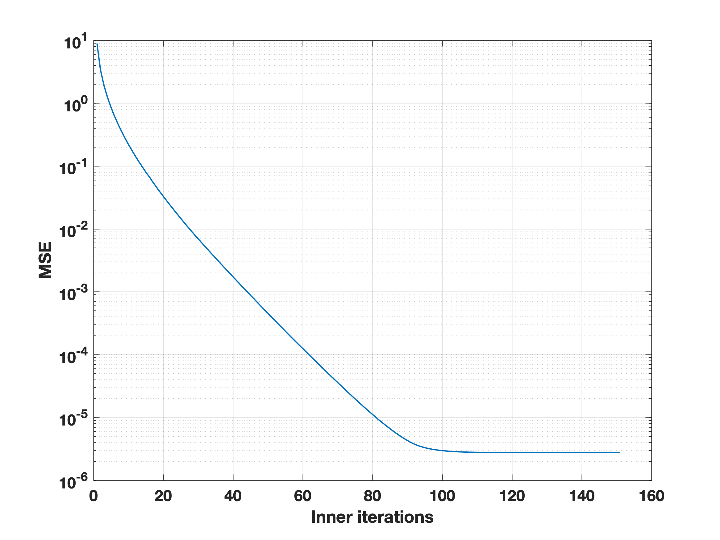
Figure 3: Synthetic $R_{1}$. (a) PRE values per iteration (b) MSE values per iteration.

The values of the computed parameters and relative errors reported in the third and fourth columns of table 3 confirm the excellent accuracy obtained by the proposed algorithm. The computed value of the regularization parameter is $\lambda^{*}=1.216\ 10^{-9}$ with computation time of $115.15\ s$.
Although the convergence of the update formula (18) depends on the initial guess $\lambda^{(0)}$, we experimentally found convergence for $\lambda^{(0)}$ in a quite large interval ($[10^{-16},10^{0}]$). In figure 4 we represent the sequences $\lambda^{(k)}$, $k=0,\ldots,15$ obtained by algorithm 2 with $\lambda^{(0)}\in\left\{10^{-16},10^{-6},10^{-4},10^{-2},10^{0}\right\}$. Optimal convergence ($k=1$) is obtained for $10^{-16}\leq\lambda^{(0)}\leq 10^{-4}$ while $\lambda^{(0)}>10^{-4}$ causes a slight increase of the iterations number, still preserving the convergence up to $\lambda^{(0)}=1$, which is usually considered as a standard starting guess. Therefore, to keep computations efficient, $\lambda^{(0)}=10^{-6}$ is used throughout the numerical experiments of this section.

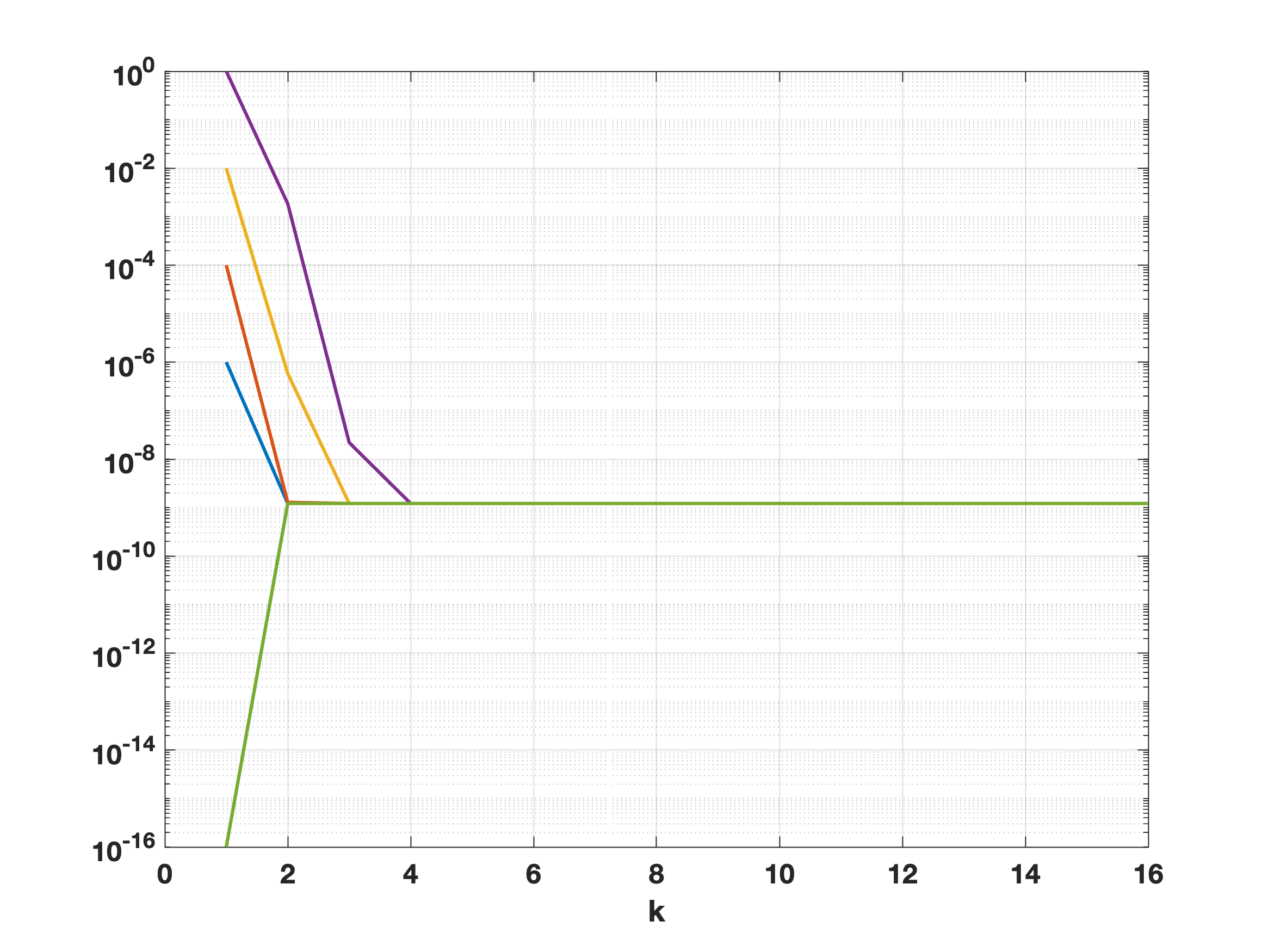
Figure 4: Synthetic $R_{1}$. Sequence $\{\lambda^{(k)}\}$, obtained by AURORA  with $\lambda^{(0)}\in\left\{10^{-16},10^{-6},10^{-4},10^{-2},10^{0}\right\}$.

Comparison with Matlab solvers

With this test problem, we aim to compare AURORA  with several methods implemented by the Matlab function fmincon: such as interior-point (ip), the active-set (as), the sequential quadratic programming (sqp) and trust-region-reflective (trr) methods. We highlight that AURORA automatically computes the value of the regularization parameter $\lambda$ while the Matlab function fmincon solves the optimization problem (7) for a fixed value of $\lambda$. Therefore, we compare the GS algorithm 1 with ip, as, sqp trr for the same fixed value $\lambda=1.\ 10^{-8}$, which we heuristically found to be a good value for all the methods.

Besides the automatic computation of the regularization parameter $\lambda$, AURORA splits the unknown parameters in two blocks and alternatively minimizes the objective function for $(R_{0},{\mathbf{f}})$, the offset and correlation distribution, and for the quadrupolar parameters $\boldsymbol{\psi}$. Two different methods are used for the solution of the corresponding sub-problems. On the contrary, fmincon computes all the parameters applying the same method.

Table 4 shows the PRE and MSE values (last row) obtained by AURORA (second column) and by the Matlab solvers, highlighting the smallest values.

	PRE
Parameter	AURORA	ip	active-set	sqp	trr
${\mathbf{f}}$	$\mathbf{4.2834\ 10^{-1}}$	1.5509	1.4497	1.3020	$8.5279\ 10^{-1}$
$R_{0}$	$\mathbf{7.0032\ 10^{-4}}$	$9.9629\ 10^{-1}$	1.0000	$2.7930\ 10^{-1}$	$1.3671\ 10^{-1}$
$C^{HN}$	$5.8238\ 10^{-5}$	4.2908	$9.6353\ 10^{-1}$	$\mathbf{1.5045\ 10^{-5}}$	$1.1591\ 10^{-2}$
$\Theta$	$\mathbf{6.9108\ 10^{-4}}$	$6.5929\ 10^{-2}$	$7.7862\ 10^{-2}$	$7.2072\ 10^{-4}$	$1.5758\ 10^{-2}$
$\Phi$	$\mathbf{8.7093\ 10^{-6}}$	$5.5535\ 10^{-1}$	2.1372	$2.6548\ 10^{-5}$	$7.2619\ 10^{-3}$
$\tau_{Q}$	$\mathbf{1.5660\ 10^{-4}}$	$9.9228\ 10^{-1}$	$3.1584\ 10^{1}$	$1.8903\ 10^{-4}$	$1.1033\ 10^{-2}$
$\nu_{-}$	$5.7679\ 10^{-6}$	$4.0856\ 10^{-1}$	$2.2756\ 10^{-1}$	$\mathbf{5.6228\ 10^{-6}}$	$5.9438\ 10^{-5}$
$\nu_{+}$	$\mathbf{1.1391\ 10^{-6}}$	$5.5197\ 10^{-2}$	$3.3362\ 10^{-2}$	$1.2084\ 10^{-6}$	$1.8516\ 10^{-5}$
$MSE$	$\mathbf{2.8131\ 10^{-6}}$	9.1906	9.0766	$3.1658\ 10^{-6}$	$2.8289\ 10^{-3}$

Table 4: Parameter relative errors and MSE of AURORA and methods implemented by the Matlab function fmincon.

The distribution ${{\mathbf{f}}}$ computed by sqp is shown in figure 5.

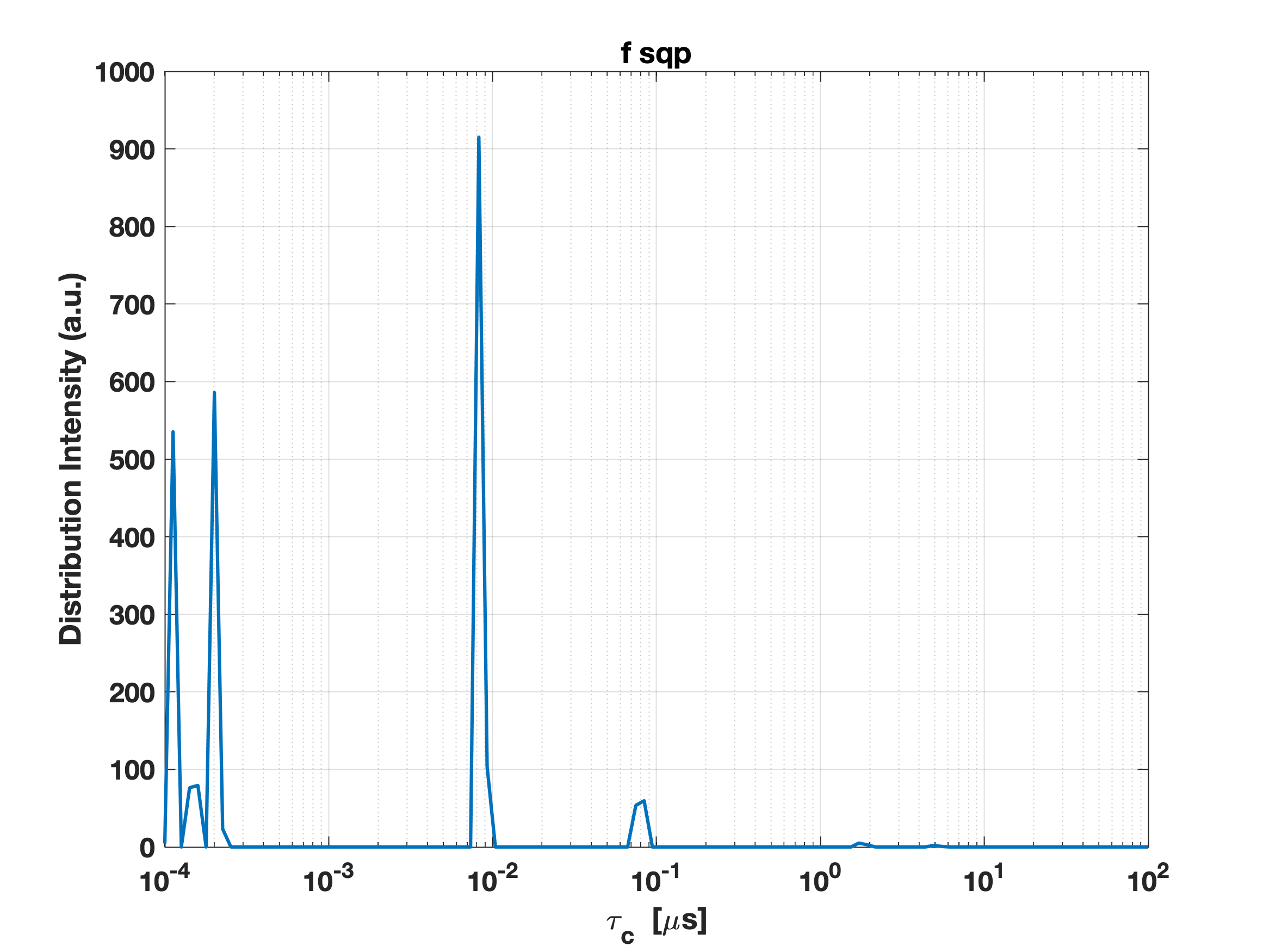
Figure 5: Correlation time distribution ${\mathbf{f}}$ computed by sqp method.

We observe that AURORA has globally superior accuracy both in data fitting and parameter estimation. Only sqp has MSE value similar to AURORA ($3.1658e-06$ compared to $2.8131e-06$), and a slightly better PRE for parameters $C^{HN}$ and $\nu_{-}$, but the amplitude distribution in figure 5 shows too many spurious peaks.

Test with noisy data

In this paragraph we test the algorithm robustness to data perturbations by computing noisy data ${\mathbf{y}}^{\delta}\in\mathbb{R}^{m}$ from a random uniformly distributed vector $\mathbf{v}\in\mathbb{R}^{m}$ with values in the interval $[-1,1]$ s.t.

$$y^{\delta}_{i}=y_{i}(1+\delta v_{i}),\ i=1,\ldots,m$$

and consider the cases $\delta=1\%,5\%,10\%$. Computing $500$ noisy samples ${\mathbf{y}}^{\delta}_{j}$ we run AURORA and compare the errors on the estimated parameters as well as reconstructed NMRD profiles.

For the noise values $\delta=1\%,5\%,10\%$, we compute the mean PRE for each parameter and represent the mean values in the bar plot shown in figure 6 together with the product $C^{HN}\cdot\tau_{Q}$.

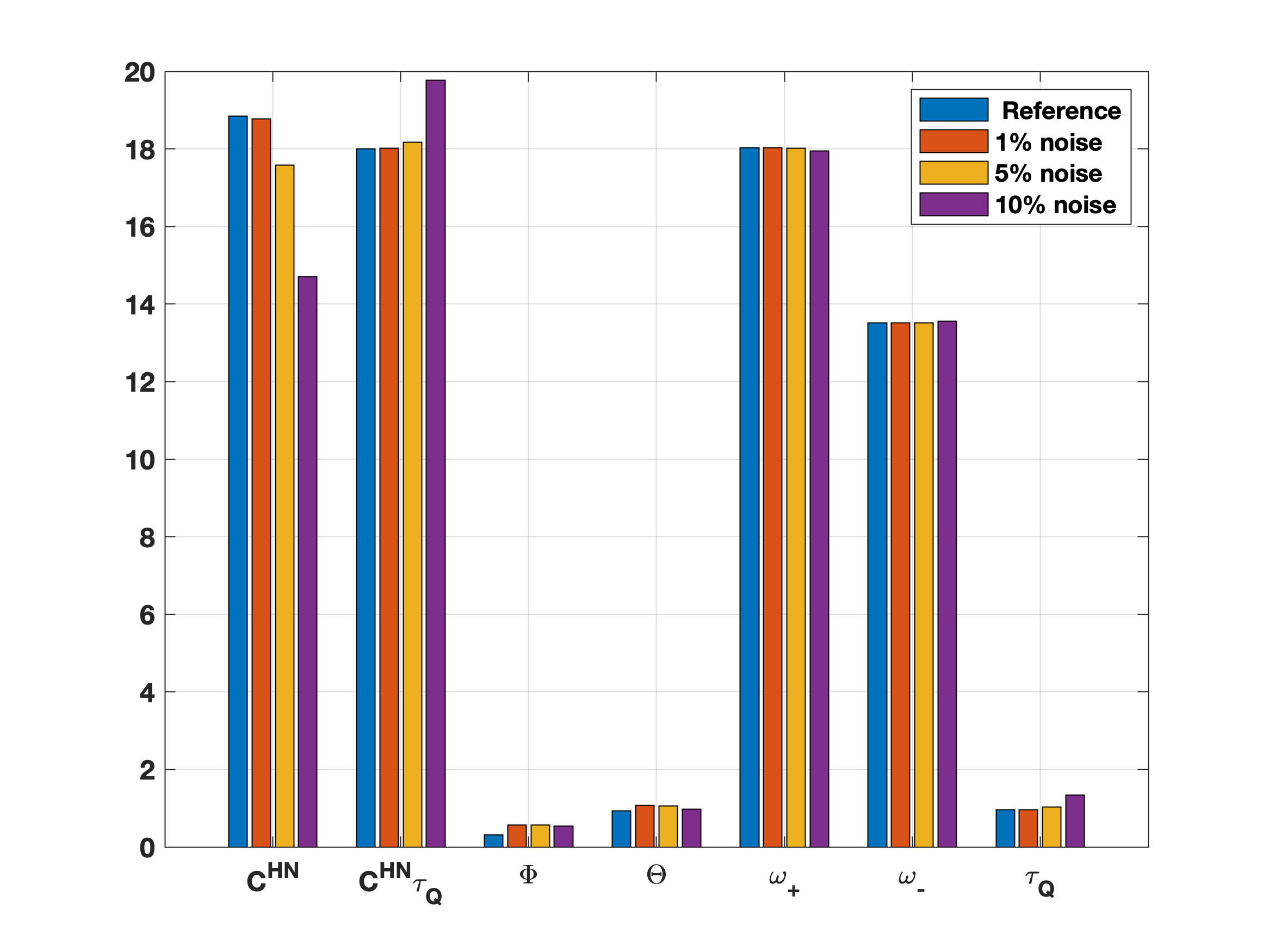
Figure 6: Mean parameter values computed by 500 noisy NMRD profiles with noise $\delta=1\%,5\%10\%$.

The mean PRE and MSE are reported in table 5.

	PRE
	$1\%$	$5\%$	$10\%$
${\mathbf{f}}$	$5.9019\ 10^{-1}$	$1.1816$	$1.4509$
$R_{0}$	$3.6393\ 10^{-2}$	$1.6726\ 10^{-1}$	$1.8099\ 10^{-1}$
$C^{HN}$	$3.3625\ 10^{-2}$	$2.7021\ 10^{-1}$	$4.7742\ 10^{-1}$
$\Theta$	$2.3023\ 10^{-2}$	$1.0678\ 10^{-1}$	$2.1726\ 10^{-1}$
$\Phi$	$3.5151\ 10^{-2}$	$4.0280\ 10^{-1}$	$6.5910\ 10^{-1}$
$\tau_{Q}$	$4.4998\ 10^{-2}$	$1.8862$	$1.1095\ 10^{1}$
$\nu_{-}$	$4.3917\ 10^{-3}$	$4.8712\ 10^{-2}$	$7.2441\ 10^{-2}$
$\nu_{+}$	$3.0889\ 10^{-3}$	$3.8712\ 10^{-2}$	$5.6856\ 10^{-2}$
MSE	$1.5980\ 10^{-1}$	3.1441	$1.0055\ 10^{1}$

Table 5: Mean PRE and MSE on 500 noisy NMRD profiles with $\delta=1\%,5\%,10\%$.

The computed $R_{1}$ curves and the zoom in the QRE interval are shown in figures 7,8 and 9 for $\delta=1\%,5\%,10\%$ respectively.

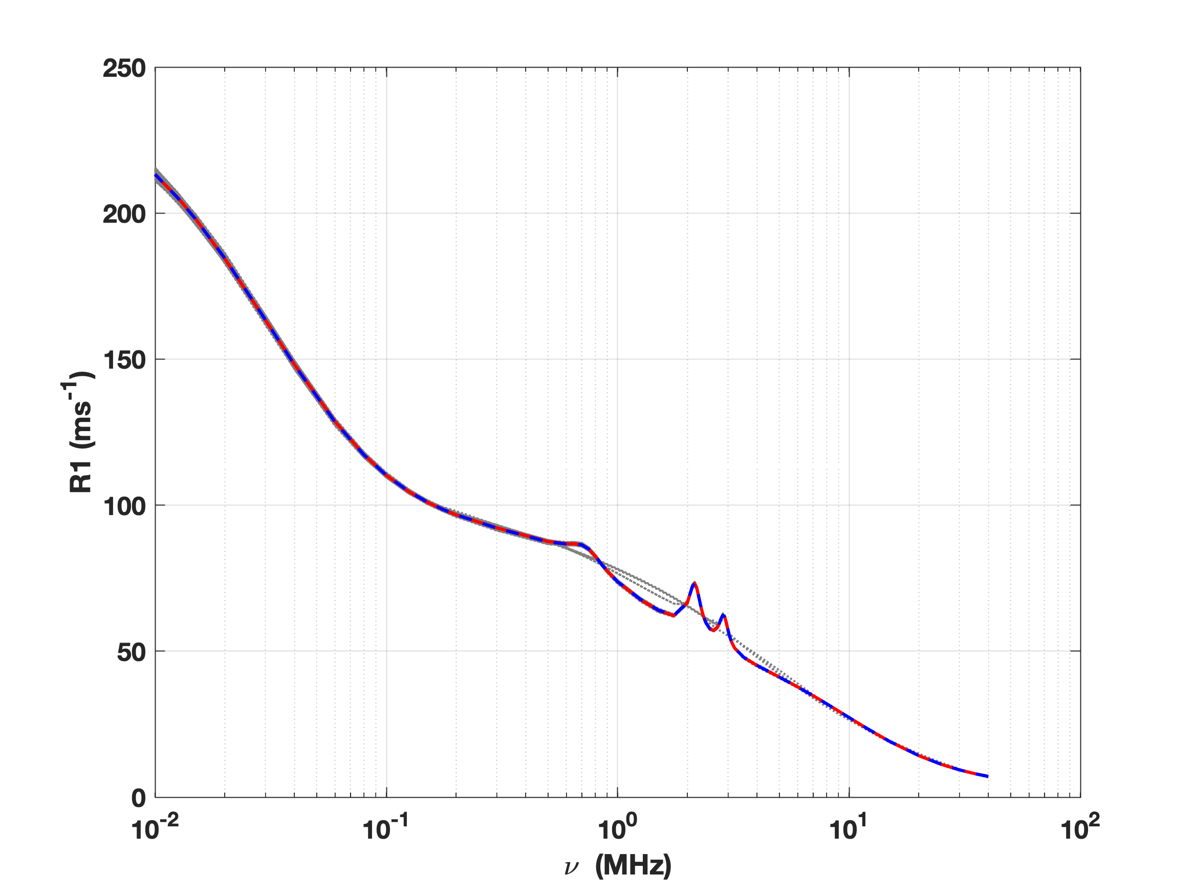
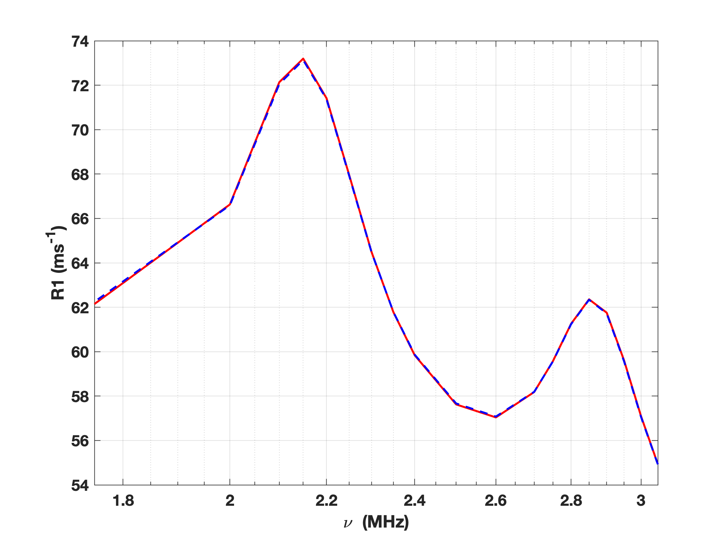
Figure 7: Fit of NMRD obtained from 500 noisy Synthetic NMRD curves with noise $\delta=1\%$. (a) Light gray: 500 fitted $R_{1}$ curves, Red line: Reference NMRD curve. Blue line: average over 500 fitted $R_{1}$ values. (b) zoom in QRE interval.

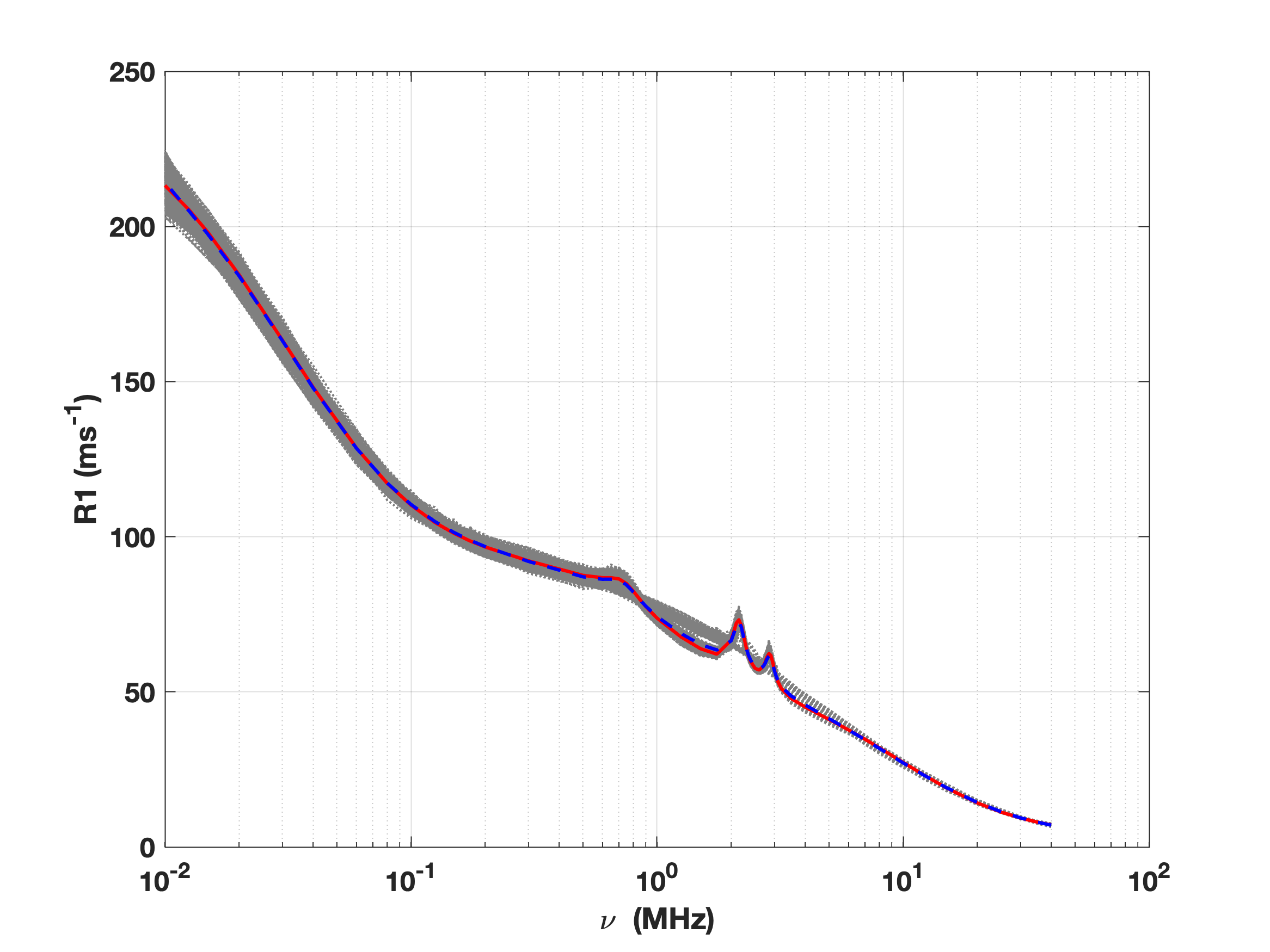
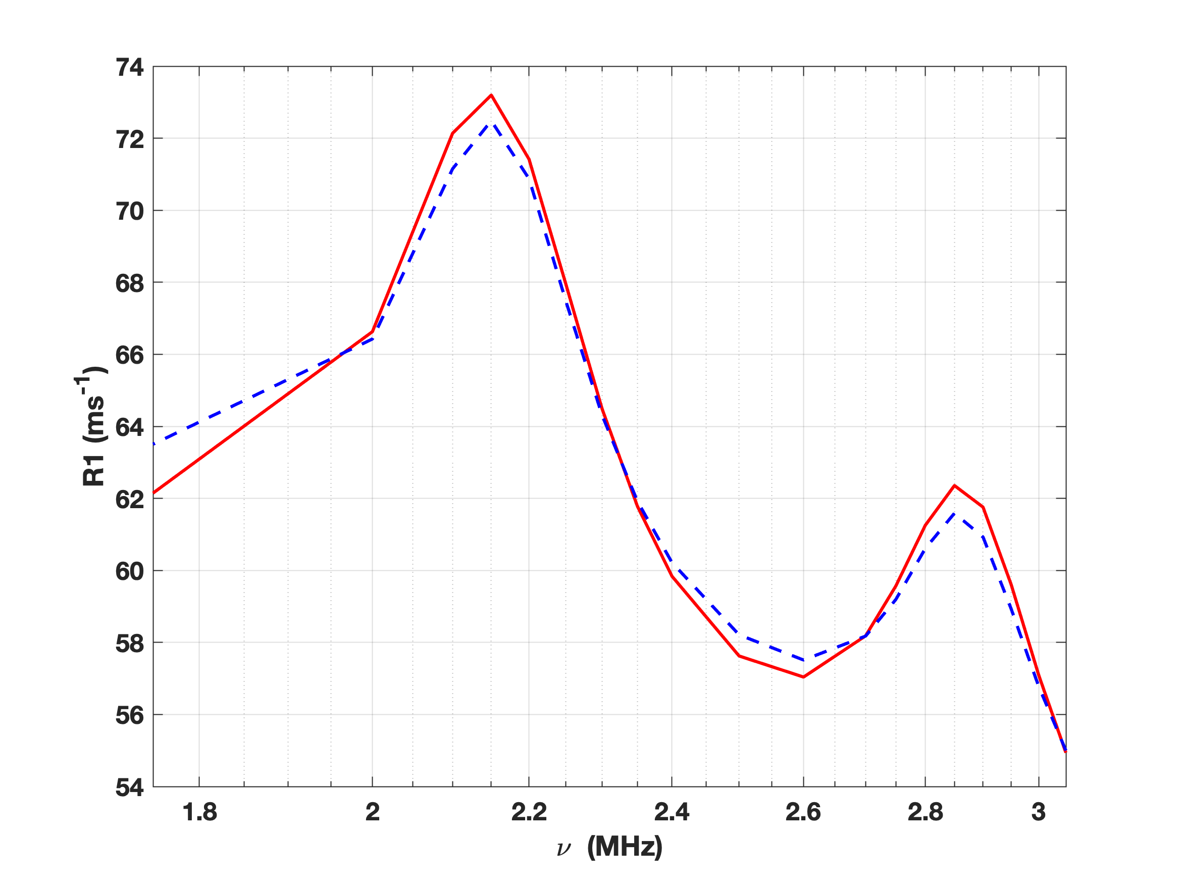
Figure 8: Fit of NMRD obtained from 500 noisy Synthetic NMRD curves with noise $\delta=5\%$. (a) Light gray: 500 fitted $R_{1}$ curves, Red line: Reference NMRD curve. Blue line: average over 500 fitted $R_{1}$ values. (b) zoom in QRE interval.

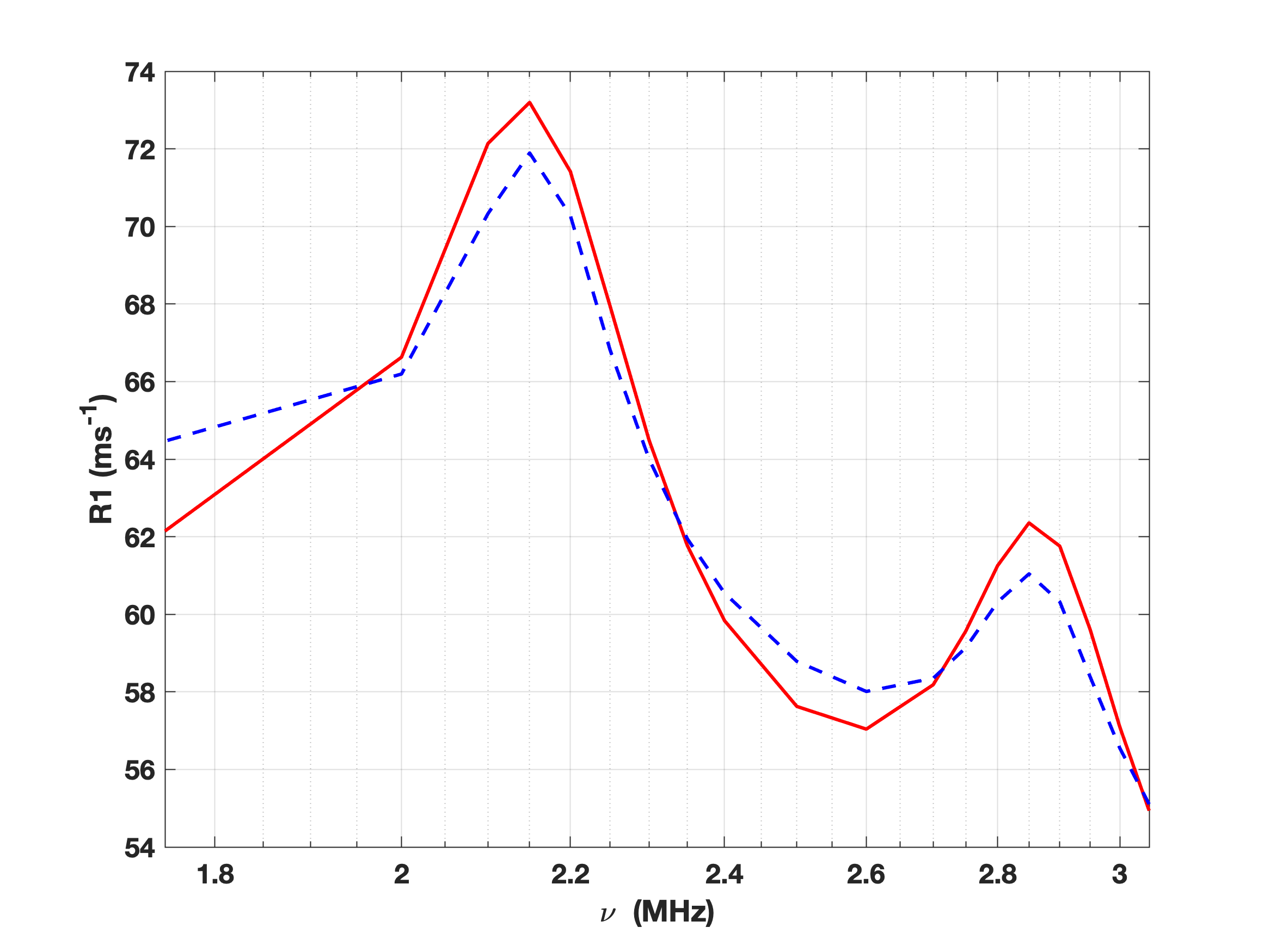
Figure 9: Fit of $R_{1}$ obtained from 500 noisy synthetic NMRD profiles with noise $\delta=10\%$. (a) Light gray: 500 fitted $R_{1}$ curves, Red line: Reference NMRD curve. Blue line: average over 500 fitted $R_{1}$ values. (b) zoom in QRE interval.

In figure 6, we observe that data noise affects mainly $C^{HN}$, $\tau_{Q}$ and $\Phi$ values. However, considering the value of the product $C^{HN}\tau_{Q}$, represented by the second group in figure 6, we see that the value is preserved when $\delta=1\%,5\%$. This feature is a physical characteristic and allows us to consider accurate the related parameters.

Although the average MSE increase with data noise, the computed average $R_{1}$ curves show a very good agreement to the reference NMRD profiles (figures 7, 8 and 9). The QRE is well reproduced even with high noise (figures 7(b), 8(b) and 9(b)).

4.3 NMRD profiles from FFC measures

In this paragraph we consider the NMRD profiles obtained from two different materials described in [13].

• A sample of 24-month aged Parmigiano-Reggiano (PR) cheese. The NMRD profile represented in figure 10(a) has $m=48$ values with confidence intervals ranging from $\pm 0.35\%$ to $\pm 3.07\%$ of the value. The quadrupolar peaks, represented in figure 11(a), correspond to frequency values $\nu_{-}=2.1$ and $\nu_{+}=2.8$ of values $R1_{-}=32.2\ s^{-1}$ and $R1_{+}=30.7\ s^{-1}$ respectively.

• Dry nanosponge (DN). In this case the NMRD profile represented in figure 10(b) has $m=44$ values with confidence intervals ranging from $\pm 0.47\%$ to $\pm 1.54\%$ of the value. The quadrupolar peaks, represented in figure 10(b), correspond to frequency values $\nu_{-}=2.4991\ MHz$ and $\nu_{+}=3.1488\ MHz$ of values $R1_{-}=104.85\ s^{-1}$ and $R1_{+}=104.85\ s^{-1}$ respectively.

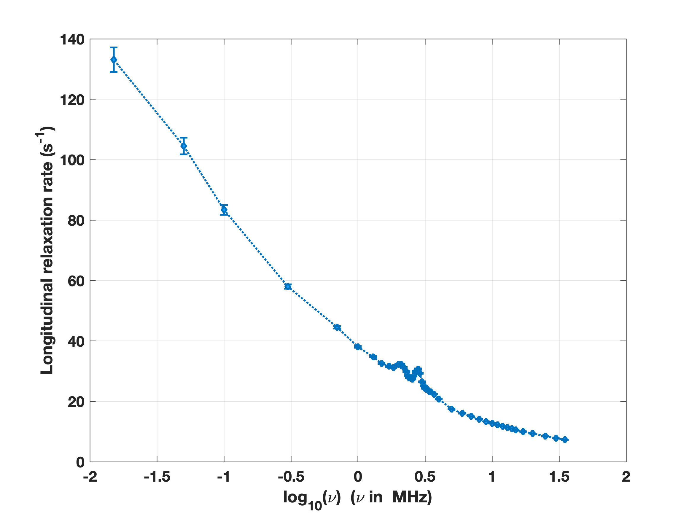
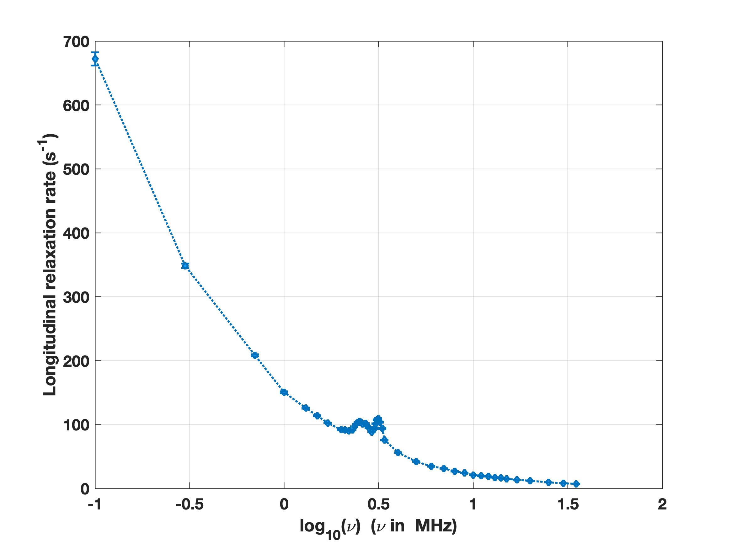
(a)                                             (b)

Figure 10: NMRD profiles. (a) Parmigiano Reggiano sample. (b) Dry nanosponge sample.

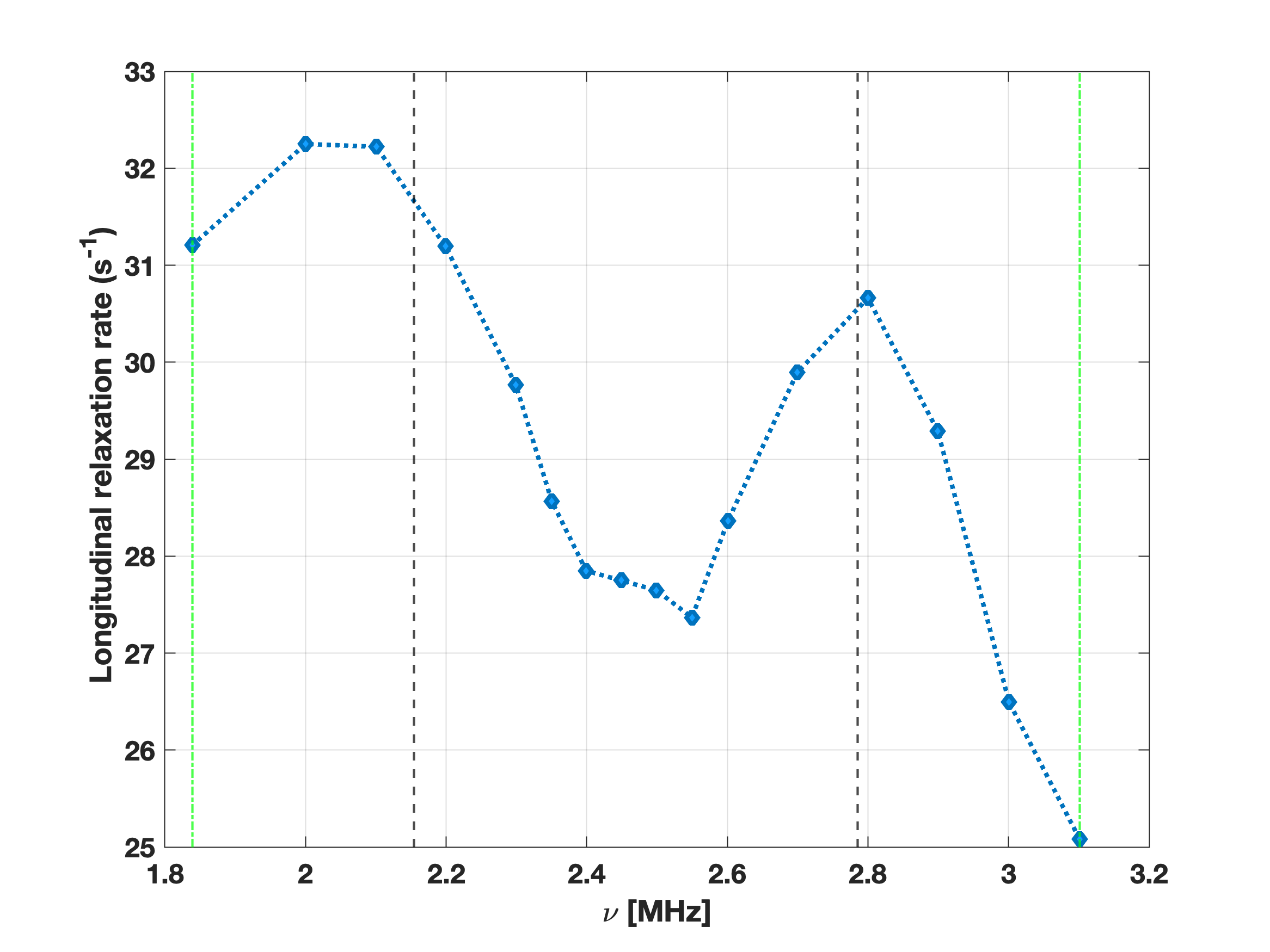
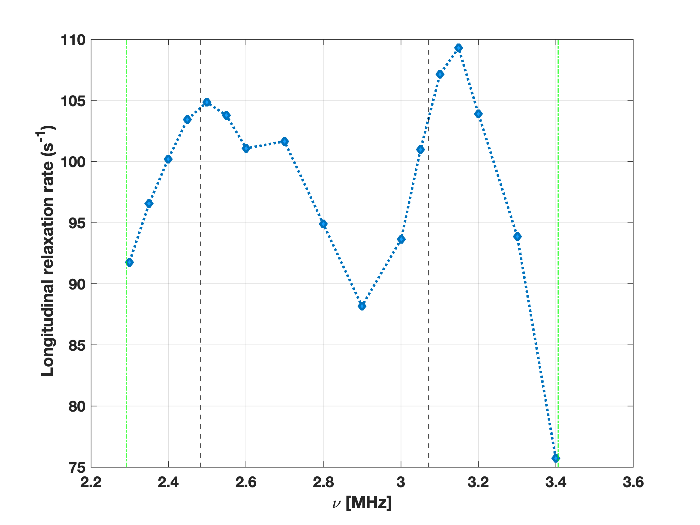
(a)                                             (b)

Figure 11: Zoom of quadrupolar dips. (a) Parmigiano Reggiano Cheese. (b) Dry nanosponge sample.

The proposed AURORA method has been used to compute the model parameters reported in table 6.

	Parameter values
	PR	DN
$R_{0}$	3.23	2.73
$C^{NH}$	5.66	69.00
$\Theta$	1.25	0.91
$\Phi$	0.86	0.87
$\tau_{Q}$	1.02	0.74
$\nu_{-}$	2.1	2.56
$\nu_{+}$	2.8	3.17
MSE	$7.8887\ 10^{-2}$	$2.7853$

Table 6: Values of the parameters fitted by AURORA and MSE in the last row.

The obtained correlation distributions are represented in figure 12 in dark green line.

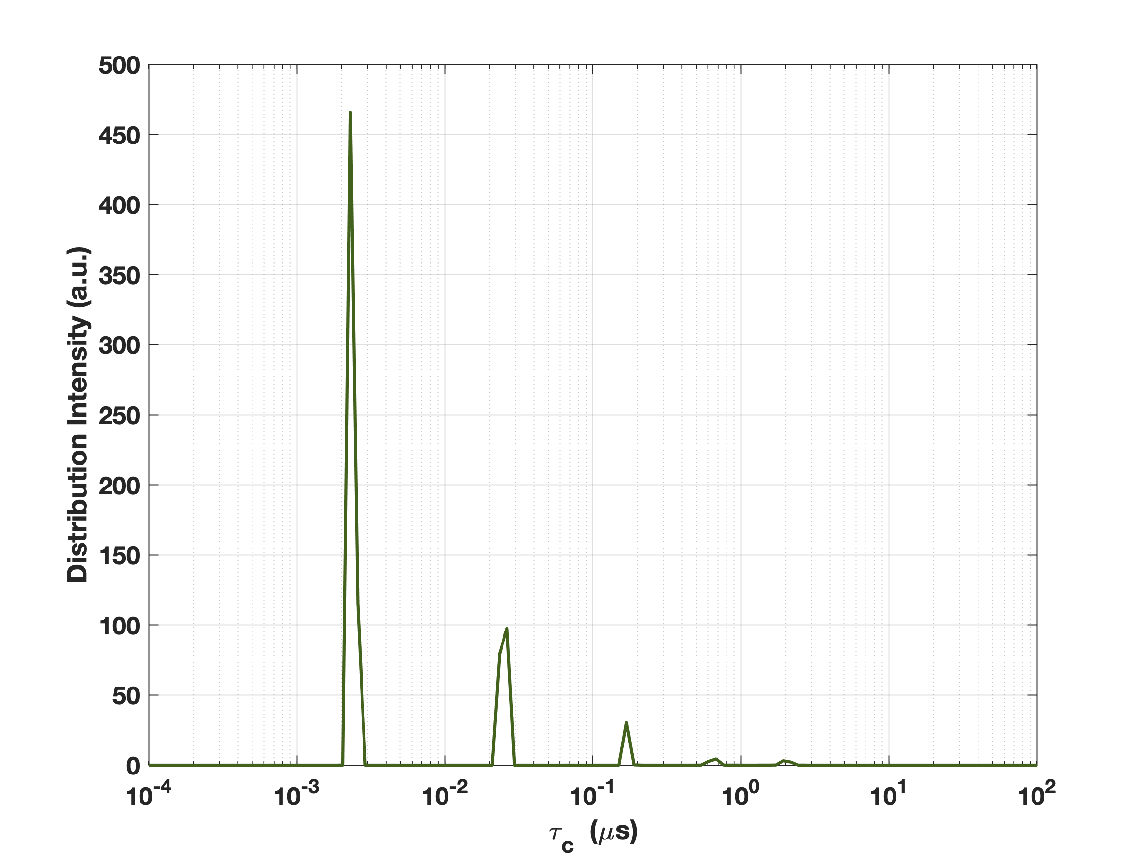
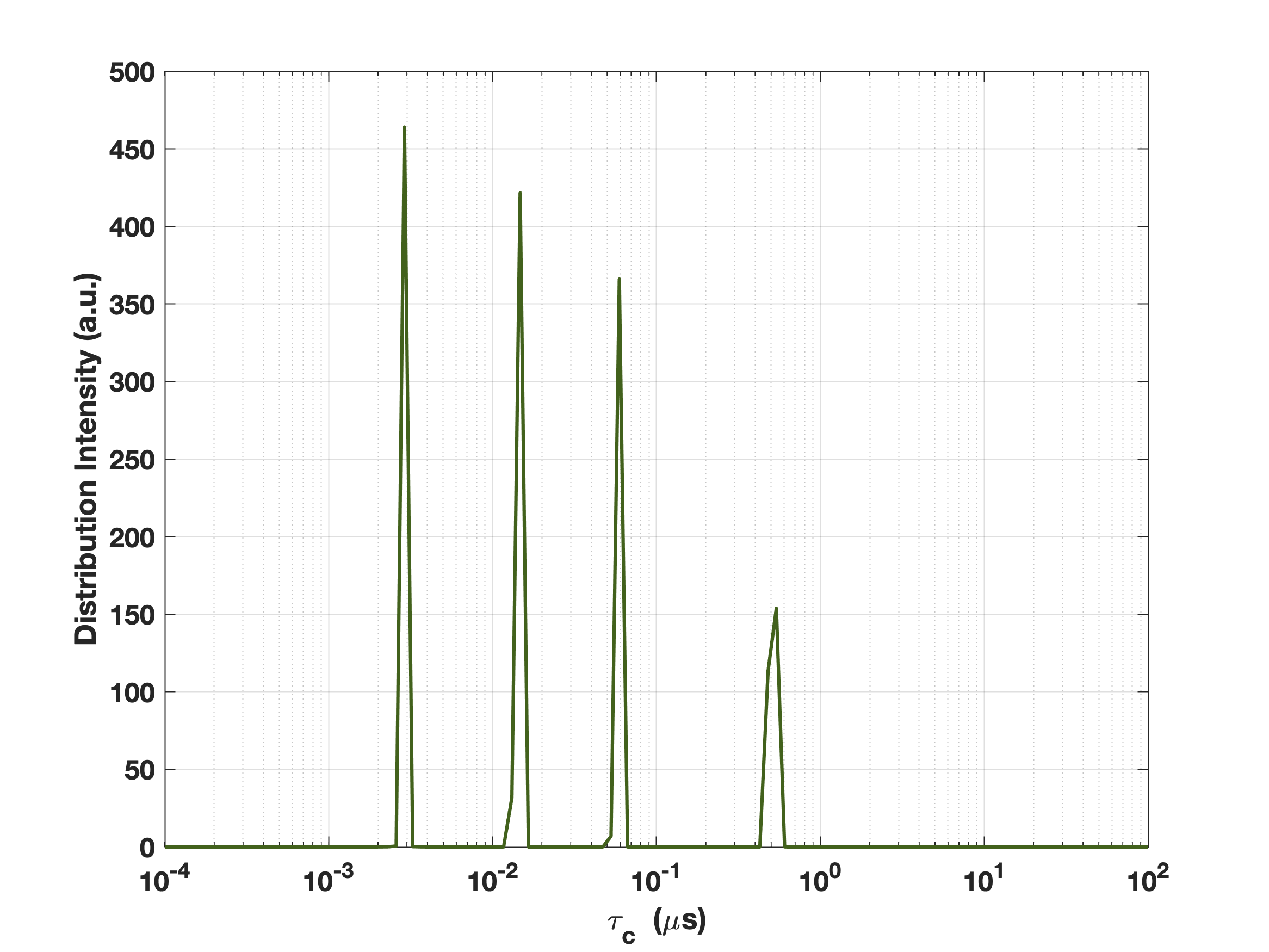
(a)                                             (b)

Figure 12: Correlation distribution (dark green lines). (a) Parmigiano Reggiano sample. (b) Dry nanosponge sample.

Concerning the fit of the NMRD profiles we measured the MSE reported in the last row of table table 6. The fitted NMRD profiles, represented in figure 13, show in blue line the data and error bars while the fitted curves are represented in red line for both samples.

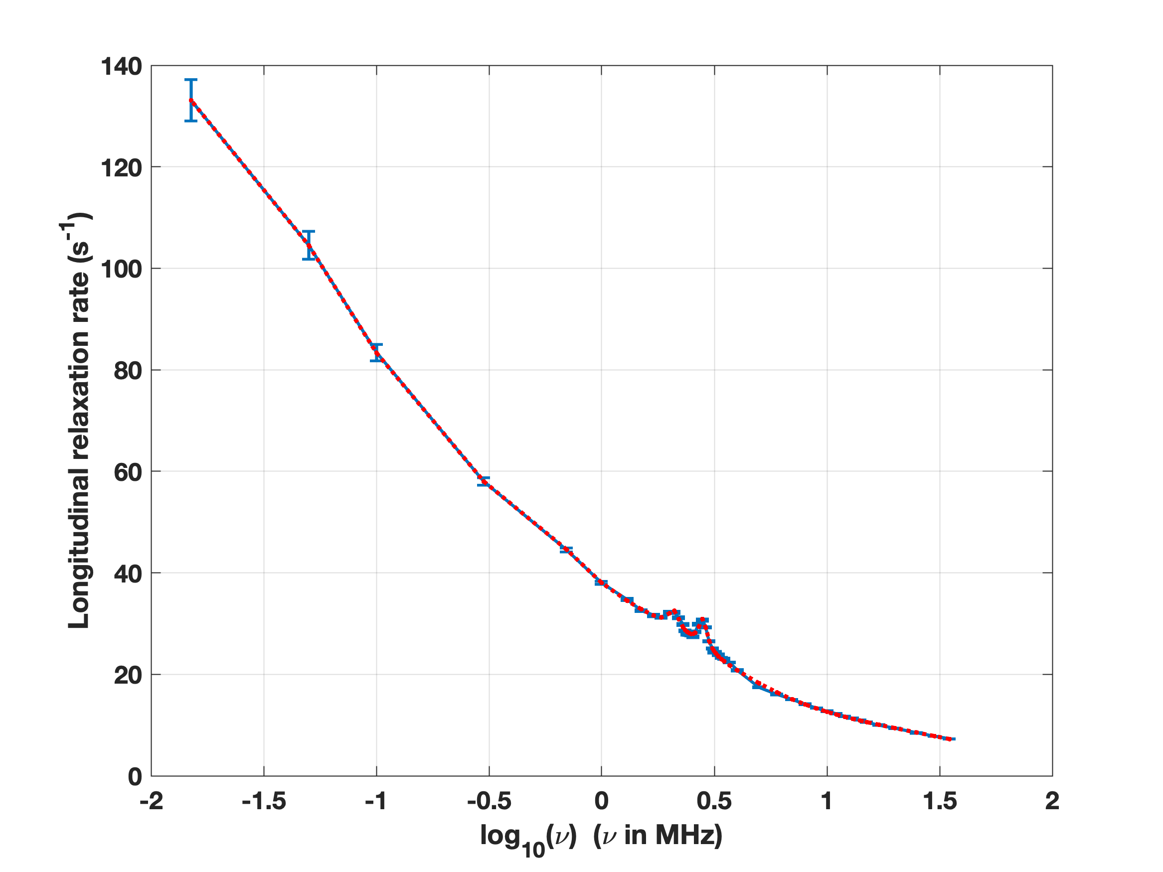
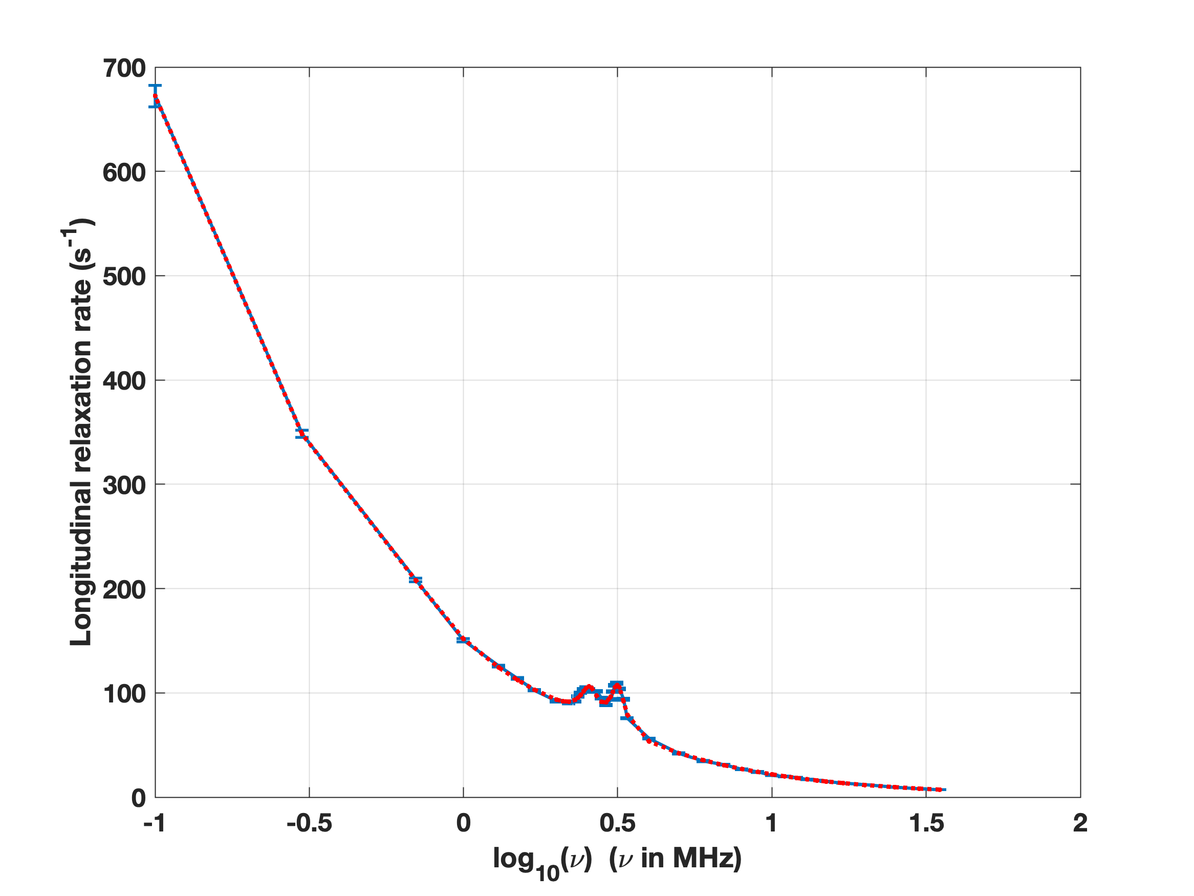
(a)                                             (b)

Figure 13: NMRD data and error bars (blue lines) and fitted curve (red lines). (a) Parmigiano Reggiano sample. (b) Dry nanosponge sample.

The zoom in the frequencies of QRE interval is shown in figure 14.

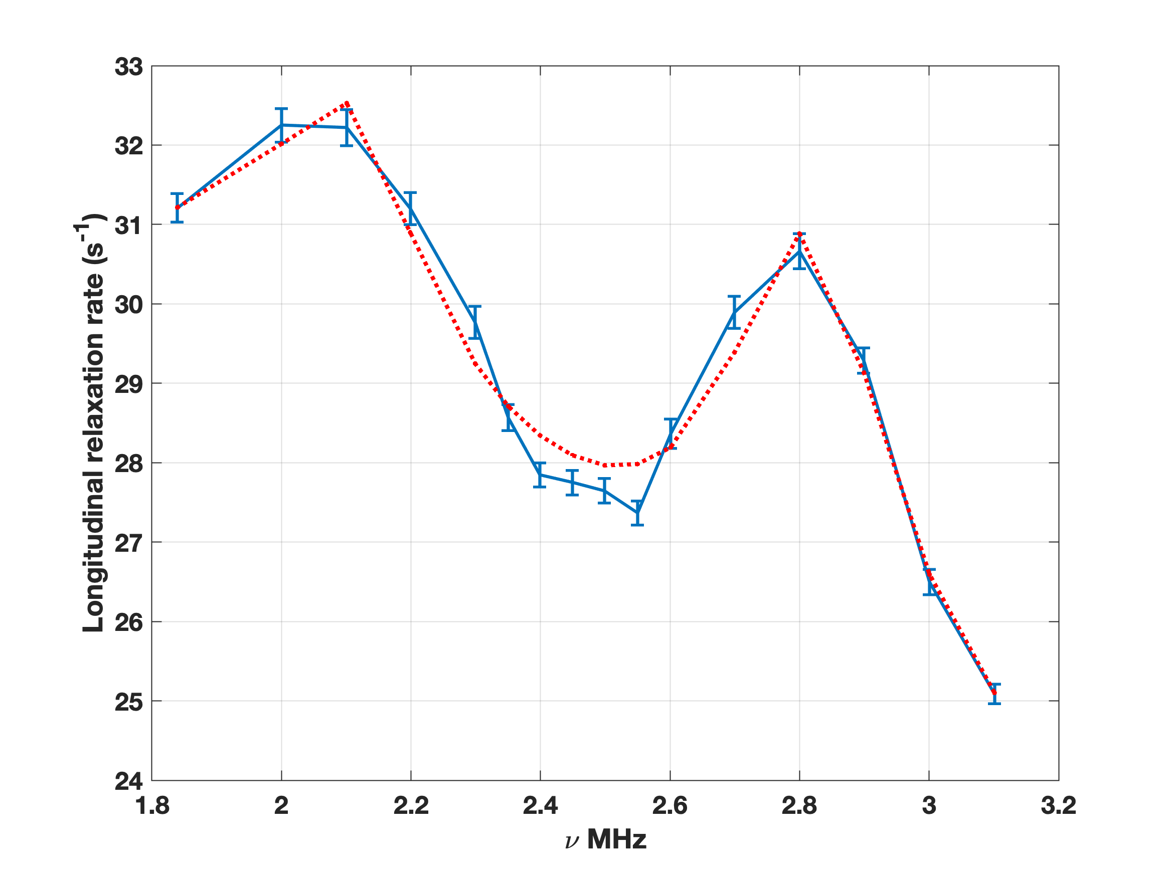
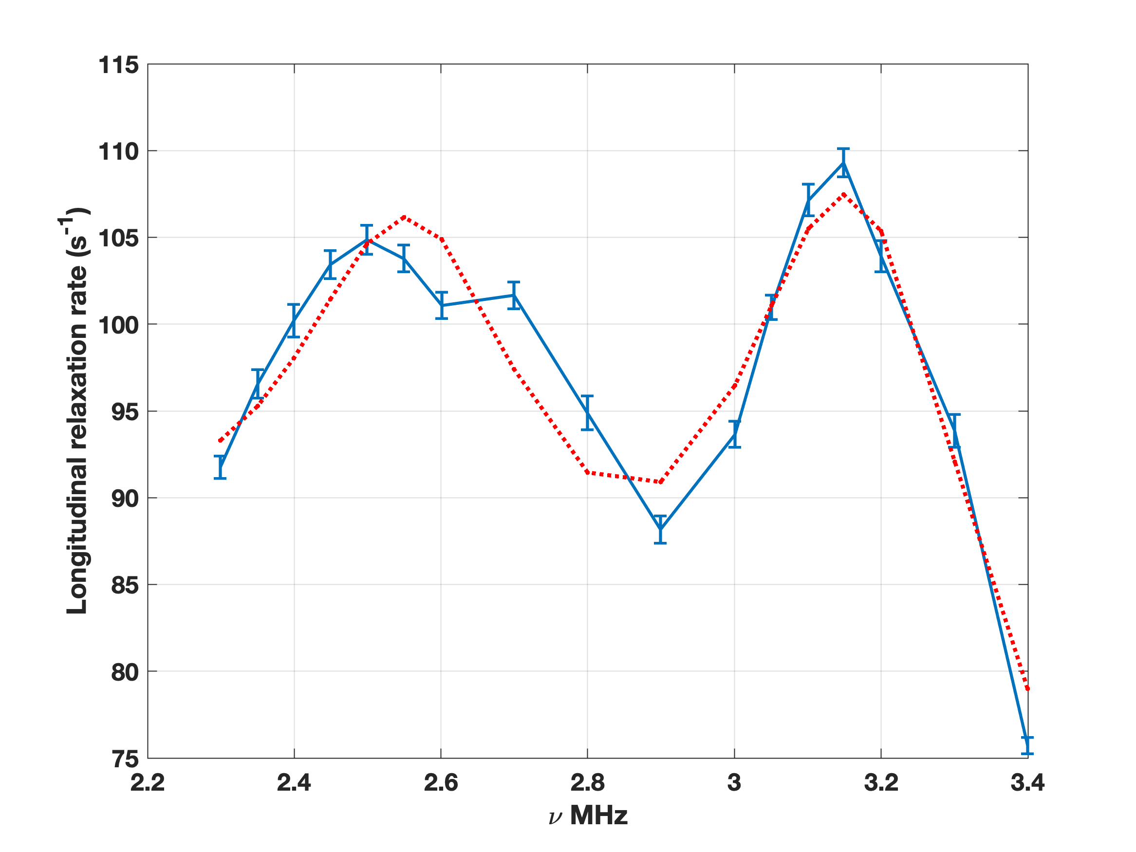
(a)                                             (b)

Figure 14: Zoom of data and fitted curves in the QRE intervals. NMRD data and error bars (blue lines) and fitted curve (red lines). (a) PR sample. (b) DN sample.

The results confirm the excellent fit to the NMRD profile (figure 13) also in the QRE interval (figure 14).

5 Conclusion

The present contribution investigates an automatic approach for analyzing the NMRD profiles in the presence of the quadrupolar relaxation enhancement. This feature yields a non-linear model whose parameters require the solution of a constrained non-linear least squares problem. Coupling the model-free approach and $L_{1}$ regularization, we tackle the constrained problem by a two-blocks non-linear Gauss-Seidel method. We assess the well-posedness of the optimization problem (existence of a minimum) and the convergence of the GS iterations to a critical point. Finally, we introduce an automatic convergent update rule of the regularization parameter based on the Balancing Principle.

The proposed algorithm is investigated both with synthetic and real data and the results state that it is a robust, fast approach to obtain accurate estimates of the correlation times distributions as well as modeling the quadrupolar function.

Moreover, we highlight that AURORA  can be viewed as a reference framework to construct parameter estimation procedures when the model parameters can be split into independent blocks allowing the use of different computational approaches for each block. In this regard, future work will include the extension of such a framework to different models of NMRD profiles where the number of correlation times $\tau$ in (2) is assigned, and their values are to be estimated together with the corresponding component ${\mathbf{f}}(\tau)$.
Given the very accurate and promising results, AURORA will be included in the Matlab software tool FreeModelFFC Tool for the inversion of NMRD profiles with QRE (available in https://site.unibo.it/softwaredicam/en/software).

References

- [1] R. Kimmich, Field-cycling NMR relaxometry, in: NMR, Springer, 1997, pp. 138–148.
- [2] P. Conte, Applications of fast field cycling NMR relaxometry, in: Annual Reports on NMR Spectroscopy, Vol. 104, Elsevier, 2021, pp. 141–188.
- [3] T. C. Farrar, E. D. Becker, Pulse and Fourier transform NMR: introduction to theory and methods, Elsevier, 2012.
- [4] P. H. Fries, E. Belorizky, Simple expressions of the nuclear relaxation rate enhancement due to quadrupole nuclei in slowly tumbling molecules, The Journal of Chemical Physics 143 (4) (2015) 044202.
- [5] D. Kruk, E. Masiewicz, A. M. Borkowska, P. Rochowski, P. H. Fries, L. M. Broche, D. J. Lurie, Dynamics of solid proteins by means of nuclear magnetic resonance relaxometry, Biomolecules 9 (11) (2019) 652.
- [6] T. Jeoh, N. Karuna, N. D. Weiss, L. G. Thygesen, Two-dimensional -nuclear magnetic resonance relaxometry for understanding biomass recalcitrance, ACS Sustainable Chemistry & Engineering 5 (10) (2017) 8785–8795.
- [7] P. Conte, L. Cinquanta, P. Lo Meo, F. Mazza, A. Micalizzi, O. Corona, Fast field cycling NMR relaxometry as a tool to monitor parmigiano reggiano cheese ripening, Food Research International 139 (2021) 109845.
- [8] E. G. Ates, V. Domenici, M. Florek-Wojciechowska, A. Gradišek, D. Kruk, N. Maltar-Strmečki, M. Oztop, E. B. Ozvural, A.-L. Rollet, Field-dependent NMR relaxometry for food science: Applications and perspectives, Trends in Food Science & Technology (2021).
- [9] J. P. Korb, Nuclear magnetic relaxation of liquids in porous media, New Journal of Physics 13 (3) (2011) 035016.
- [10] J. Mitchell, L. M. Broche, T. C. Chandrasekera, D. J. Lurie, L. F. Gladden, Exploring surface interactions in catalysts using low-field nuclear magnetic resonance, The Journal of Physical Chemistry C 117 (34) (2013) 17699–17706.
- [11] D. A. Faux, P. J. McDonald, Explicit calculation of nuclear-magnetic-resonance relaxation rates in small pores to elucidate molecular-scale fluid dynamics, Physical Review E 95 (3) (2017) 033117.
- [12] D. Kruk, P. Rochowski, M. Florek-Wojciechowska, P. J. Sebastião, D. J. Lurie, L. M. Broche, spin-lattice NMR relaxation in the presence of residual dipolar interactions–dipolar relaxation enhancement, Journal of Magnetic Resonance 318 (2020) 106783.
- [13] P. Lo Meo, S. Terranova, A. Di Vincenzo, D. Chillura Martino, P. Conte, Heuristic algorithm for the analysis of fast field cycling (ffc) NMR dispersion curves, Analytical Chemistry (2021).
- [14] B. Halle, H. Jóhannesson, K. Venu, Model-free analysis of stretched relaxation dispersions, Journal of Magnetic Resonance 135 (1) (1998) 1–13.
- [15] B. Halle, The physical basis of model-free analysis of NMR relaxation data from proteins and complex fluids, The Journal of chemical physics 131 (22) (2009) 224507.
- [16] K. Ito, B. Jin, T. Takeuchi, A regularization parameter for nonsmooth Tikhonov regularization, SIAM Journal on Scientific Computing 33 (3) (2011) 1415–1438.
- [17] L. Grippo, M. Sciandrone, Globally convergent block-coordinate techniques for unconstrained optimization, Optimization Methods and Software 10 (4) (1999) 587–637.
- [18] L. Grippo, M. Sciandrone, On the convergence of the block nonlinear gauss–seidel method under convex constraints, Operations Research Letters 26 (3) (2000) 127–136. doi:https://doi.org/10.1016/S0167-6377(99)00074-7.
- [19] D. Bertsekas, Nonlinear Programming, Athena Scientific, (2nd Edition), 1999.
- [20] S.-J. Kim, K. Koh, M. Lustig, S. Boyd, D. Gorinevsky, An interior-point method for large-scale -regularized least squares, IEEE Journal of Selected Topics in Signal Processing 1 (4) (2007) 606–617.
- [21] D. Bertsekas, Projected Newton methods for optimization problems with simple constraints, SIAM Journal on Control and Optimization 20 (2) (1982) 221–246.
- [22] E. Gafni, D. Bertsekas, Two-metric projection methods for constrained optimization, SIAM Journal on Control and Optimization 22 (6) (1984) 936–964.
- [23] J. Nocedal, S. J. Wright, Numerical Optimization, 2nd Edition, Springer, New York, NY, USA, 2006.
- [24] H. Engl, M. Hanke, A. Neubauer, Regularization of Inverse Problems, Springer Dordrecht, 2000.
- [25] H. P. Christian, Rank-deficient and discrete ill-posed problems, SIAM Monographs on Mathematical Modeling and Computation, Society for Industrial and Applied Mathematics (SIAM), Philadelphia, PA, 1998.
- [26] C. Vogel, Computational Methods for Inverse Problems, Vol. 23 of Frontiers in Applied Mathematics, SIAM, 2002.
- [27] T. Bonesky, Morozov’s discrepancy principle and Tikhonov-type functionals, Inverse Problems 25 (1) (2008) 015015.
- [28] C. Clason, B. Jin, A semismooth Newton method for nonlinear parameter identification problems with impulsive noise, SIAM Journal on Imaging Sciences 5 (2) (2012) 505–536.