Recovering the Graph Underlying Networked Dynamical Systems
under Partial Observability: A Deep Learning Approach

Abstract

We study the problem of graph structure identification, i.e., of recovering the graph of dependencies among time series. We model these time series data as components of the state of linear stochastic networked dynamical systems. We assume partial observability, where the state evolution of only a subset of nodes comprising the network is observed. We propose a new feature-based paradigm: to each pair of nodes, we compute a feature vector from the observed time series. We prove that these features are linearly separable, i.e., there exists a hyperplane that separates the cluster of features associated with connected pairs of nodes from those of disconnected pairs. This renders the features amenable to train a variety of classifiers to perform causal inference. In particular, we use these features to train Convolutional Neural Networks (CNNs). The resulting causal inference mechanism outperforms state-of-the-art counterparts w.r.t. sample-complexity. The trained CNNs generalize well over structurally distinct networks (dense or sparse) and noise-level profiles. Remarkably, they also generalize well to real-world networks while trained over a synthetic network – namely, a particular realization of a random graph.

Introduction

Networked dynamical systems are characterized by a set of interconnected nodes or agents. The state of the nodes evolves over time according to their peer-to-peer interactions constrained by a support network of contacts (Barrat, Barthélemy, and Vespignani 2012; Liggett 2005; Robert 2003; Porter and Gleeson 2016). More concretely, the state of a node $i$ is only immediately affected by the state of nodes that directly link to $i$, i.e., nodes that bear a direct causal effect on node $i$. This causal network is captured by a graph, which is often a latent structure underlying these systems.

Examples of networked dynamical systems include: $i$) Pandemics – the fraction of infections within each community of individuals is captured by a time series that is strongly influenced by contacts in neighboring communities. Knowledge of the contact network (which determines the main avenues of contagion) is critical for designing effective mitigation measures (Lahmanovich and James 1976; Ganesh, Massoulié, and Towsley 2005; Santos, Moura, and Xavier 2015; Braunstein et al. 2016; Ren et al. 2019). For example, a natural mitigation policy is network dismantling: aiming to quarantine a minimal set of nodes to promote a maximal disconnect of the underlying contagion network (Braunstein et al. 2016; Ren et al. 2019) – thus, hindering virus propagation across communities without disrupting the global function of the networked system; $ii$) Brain activity – based on temporal signals gathered from cranial probes, an important task is to infer the so-called Functional Connectivity Matrix, which represents the graph of interactions among the active regions of the brain (see, e.g., (Liégeois et al. 2020)). Recent evidence shows that the Functional Connectivity Matrix can be used to diagnose or predict the onset of motor activities or cognitive disorders (Douw et al. 2010; Ranasinghe et al. 2014; Oltra et al. 2021; Stam et al. 2007; Monajemi et al. 2016; van Mierlo et al. 2019; Lehnertz, Bröhl, and Rings 2020); $iii$) Finance – the dynamics of stock prices can be influenced by interactions between firms, and knowledge of this interaction network can inform government interventions, for instance (Fenn et al. 2009, 2012; Bazzi et al. 2016).

In most practical instances of the examples above, the node-level time series are readily accessible, but the underlying causal network – which is of fundamental importance in downstream tasks – is fully or partially unknown. To address this issue, a growing body of literature has developed methods for reconstructing the network from the observed node-level time series (Chen, Wang, and Shen 2022; Pereira, Ibrahimi, and Montanari 2010; Materassi and Salapaka 2015; Matta, Santos, and Sayed 2020). In this work, we focus on linear stochastic networked dynamical systems, which is arguably one of the most natural settings for network identification from time series since a great class of nonlinear networked dynamical systems can be addressed via linearization about the equilibria under small-noise regimes (Ching and Tam 2017; Napoletani and Sauer 2008) or via appropriate embedding in higher dimensional spaces (Lim et al. 2015; Mauroy and Goncalves 2016). Moreover, since it is typically impractical to monitor all node-level signals in large-scale systems, we assume a partial observability setting, wherein we observe the time series corresponding to a small subset of nodes and aim to reconstruct the corresponding subgraph connecting them using a small number of samples. This task is much more challenging than the full observability case, since the time series of the observed nodes are also affected by the unobserved dynamics of the remainder of the network. Fig. 1 summarizes the structure identification framework considered.

This work departs from the standard approach of reconstructing networks based on scalar measures between time series – i.e., measures that assign a real-value to the coupling-strength between nodes, e.g., correlation, Granger, Precision matrix, etc. – which dates back to (Chow and Liu 1968). We propose a novel feature vector based setting constructed for each pair of nodes from their time series. In this novel setting, structure identification leverages the separability properties of the proposed feature vectors in a higher-dimensional space. We provide rigorous theoretical results proving that our features are linearly separable for any undirected network, once sufficiently many samples are taken. This provides the explainability of the method: our features can be readily used as input to a variety of machine learning pipelines to perform causal inference. We demonstrate that CNNs trained with our features outperform state-of-the-art methods in terms of accuracy and sample complexity.

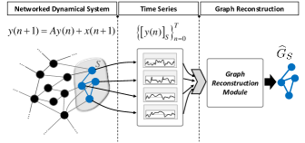
Figure 1: Structure identification under partial observability.

Related Work

Causal inference relies on the nature of the samples, and it depends on whether the observed time series are drawn independently from multivariate distributions (often assumed i.i.d. within the scope of graphical models), or are time series stemming from some networked dynamical law (not i.i.d.). For the multivariate case, the Markov property establishes a one-to-one correspondence between certain probability distributions and the set of (possibly directed) graphs (Hammersley and Clifford 2021; Pearl 2009). If $X$ is conditionally independent of $Z$ given $Y$, then there is no arrow, or direct causal effect, from $Z$ to $X$. The dependence relationships are thus captured by a graph. This Markov property can be extended to discrete-time networked dynamical systems: the state of a node at instant $n+1$ depends only on the state of some nodes at time $n$ (also known as neighbors or parents). The general goal of causal inference is to uncover the possible avenues of information flow: to recover from observation of the time series samples the underlying graph structure of dependencies defined by the Markov property. Typically, this is done by leveraging various forms of scalar measures between time series, e.g., transformations of the covariance matrix; regression (e.g., Granger estimator) (Geiger et al. 2015; Pereira, Ibrahimi, and Montanari 2010; Matta, Santos, and Sayed 2020); or other scalar graph metrics (Materassi and Salapaka 2015). The performance of the precise method ties strongly to the data generative process and to whether the system is fully or partially observed.

Full-Observability

Graphical models. Classical algorithms (assuming i.i.d. samples) based on conditional independence tests, include the SGS (Spirtes, Glymour, and Scheines 2000), PC (Spirtes and Glymour 1991), GES (Chickering 2003), and FGS (Ramsey et al. 2016). The algorithms and sufficient conditions for consistency devised in these works rely on sparsity related structural constraints that hardly fit the connectivity pattern of general networks. The work (Anandkumar et al. 2012) offers an approach for the large scale setting under certain complying assumptions of sparsity. The independence tests are leveraged via conditional covariance tests. All structural constraints, revolving around sparsity, play a critical role to render the scaling of the independence tests amenable to computation, otherwise, the problem becomes quickly unfeasible (Bresler, Gamarnik, and Shah 2014; Bogdanov, Mossel, and Vadhan 2008).

Networked dynamical systems. For approaches in the signal processing literature, (Mateos et al. 2019) provides an overview highlighting regression plus regularization of the network sparsity methods for full-observability over distinct models – primarily promoting sparsity of the latent network, – including linear dynamical systems as vector autoregressive (VAR) models, as in (Mei and Moura 2017; Moneta et al. 2009; Kivits and Hof 2022). In this regard, (Pereira, Ibrahimi, and Montanari 2010) addresses the problem for linear stochastic differential equations (SDEs) via an optimization formulation that regularizes sparsity of the latent network. This problem is addressed by first converting the continuous-time SDE into a discrete-time linear dynamical system – a technique that yields the discrete-time model considered in this work. Other schemes exploit spectral-based methods (Granger 1969; Segarra, Schaub, and Jadbabaie 2017; Segarra et al. 2017). These leverage the spectral properties of the interaction matrix or support graph (Sandryhaila and Moura 2013) to characterize signatures that allow consistent estimation over certain sparse networks.

Partial-Observability

Graphical models. In general, the proposed approaches rely on conditional independence (CI) tests or measures thereof, e.g., conditional mutual information (CMI) or transfer entropy, and a causal link is declared whenever a test yields a positive CMI-based metric. Classical algorithms for causal inference under the presence of latent variables are the FCI (Spirtes, Meek, and Richardson 1995) and RFCI (Colombo et al. 2012). As in the full-observability setting, consistent tests scale combinatorially with the connectivity of the causal graph, rendering the CI-based approaches impractical for denser graphs. To control the curse of connectivity, CI-based methods often act at a microscopical level relying on several strong structural constraints including, directed acyclic graphs, long girth (Anandkumar et al. 2013; Anandkumar and Valluvan 2013) and other more technical local structural conditions, such as bottleneck and non-redundancy (Adams, Hansen, and Zhang 2021; Mastakouri, Schölkopf, and Janzing 2021).

Networked dynamical systems. In (Materassi and Salapaka 2015; Materassi and Salapaka 2012a, b), linear dynamical systems are addressed via certain pseudo-metrics, e.g. log-coherence distance, aiming to capture the true graph-distance between nodes. In (Geiger et al. 2015) some conditions on the network connectivity and interaction matrix of a linear networked dynamical system are proposed, in order to obtain uniqueness of the network connectivity given partially observed samples. It does not provide, however, an algorithm with consistency guarantees to retrieve the uniquely determined network. On the other hand, the work (Zhao and Wan 2022) uses an expectation-maximization based approach to address certain discrete-time discrete state-space networked dynamical systems, while (Chandrasekaran, Parrilo, and Willsky 2012; Jalali and Sanghavi 2012; Mei and Moura 2018) resort to convex optimization based methods for regularizing the sparsity of the network under partial observability. The works (Santos, Matta, and Sayed 2020; Matta, Santos, and Sayed 2020, 2022) establish structural consistency of the Granger (or regression) and other matrix-valued estimators over partially observed discrete-time linear stochastic networked dynamical systems with symmetric interaction matrices, for distinct regimes of network connectivity (including densely connected networks). Similar to (Anandkumar and Valluvan 2013), the structural consistency of these estimators is established in the thermodynamic limit, i.e., as the number of nodes scales to infinite, which fits the framework of large-scale networks. Recently, (Chen, Wang, and Shen 2022) proved that the underlying interaction matrix, up to a multiplicative constant related to the noise level, can be expressed as a linear combination of covariance matrices, with high probability, under the following regime: $i$) the interaction matrix $A$ is symmetric; $ii$) the noise $\mathbf{x}$ is diagonal and homogeneous, i.e., its covariance matrix is a multiple of the identity matrix. Theorem $1$ in (Chen, Wang, and Shen 2022) will be used in the present work to establish an important result regarding the proposed set of feature vectors, namely, consistent linear separability. This property will further yield a competitive performance for the trained CNNs in terms of sample-complexity.

Problem Formulation

We consider the linear networked dynamical law

$$\mathbf{y}(n+1)=A\mathbf{y}(n)+\mathbf{x}(n+1),$$ (1)

where $\mathbf{y}(n)=\left[y_{1}(n)\,\,y_{2}(n)\,\,\ldots\,\,y_{N}(n)\right]^{\top}\in\mathbb{R}^{N}$ represents the state-vector of the $N$-dimensional networked dynamical system at time $n$ that collects the states $y_{i}(n)$ of each node $i$ at time $n$; $\mathbf{x}(n)\sim\mathcal{N}\left(0,\sigma^{2}I_{N}\right)$ represents the excitation noise associated with the $N$ nodes of the system with covariance matrix $\sigma^{2}I_{N}$, and independent across time $n$; $A\in\mathbb{R}_{+}^{N\times N}$ refers to the non-negative interaction matrix whose support represents the underlying graph linking the nodes. The dynamical system is assumed to be stable, i.e., $\rho(A)<1$, where $\rho(A)$ stands for the spectral radius of $A$.

This work deals with the problem of recovering the support of the submatrix $A_{S}$, i.e., the graph structure of connections among the observed nodes in the subset $S$ from observation of the subvector $\left[\mathbf{y}(n)\right]_{S}=\left[\mathbf{y}_{m_{1}}(n)\,\,\mathbf{y}_{m_{2}}(n)\,\,\ldots\,\,\mathbf{y}_{m_{\left|S\right|}}(n)\right]^{\top}\in\mathbb{R}^{\left|S\right|}$ over time $n$, where $\left|S\right|$ is the cardinality of the subset $S$ (see Fig.1).

Notation: $S=\left\{m_{1},m_{2},\ldots,m_{\left|S\right|}\right\}\subset\left\{1,2,\ldots,N\right\}$ is a nonempty subset of indexes with $m_{1}<m_{2}<\ldots<m_{\left|S\right|}$ and $\left|S\right|\leq N$; given a vector $\mathbf{y}\in\mathbb{R}^{N}$, $\left[\mathbf{y}\right]_{S}=\left[\mathbf{y}_{m_{1}}(n)\,\,\mathbf{y}_{m_{2}}(n)\,\,\ldots\,\,\mathbf{y}_{m_{\left|S\right|}}(n)\right]^{\top}$ is the subvector obtained from $\mathbf{y}$ and indexed by $S$; accordingly, a similar notation is adopted for matrices, namely, given $A\in\mathbb{R}^{N\times N}$, the matrix $A_{S}\in\mathbb{R}^{\left|S\right|\times\left|S\right|}$ or $\left[A\right]_{S}\in\mathbb{R}^{\left|S\right|\times\left|S\right|}$ is defined as the submatrix whose $ij^{\text{th}}$ entry is $A_{m_{i}m_{j}}$; ${\sf Supp}\left(A\right)$ is the support of the matrix $A$, i.e., $\left[{\sf Supp}\left(A\right)\right]_{ij}=\mathbf{1}_{\left\{A_{ij}\neq 0\right\}}$; $\left|\left|\mathbf{y}\right|\right|_{\infty}$ refers to the $L_{\infty}$-norm that returns the maximal absolute value across the entries of the vector $\mathbf{y}\in\mathbb{R}^{N}$; the set of natural numbers, including zero, is denoted by $\mathbb{N}=\left\{0,1,2,\ldots\right\}$.

Structural Consistency

Consider the following $k^{\text{th}}$ lag covariance matrix

$$R_{k}(n)\overset{\Delta}{=}\mathbb{E}\left[\mathbf{y}(n+k)\mathbf{y}(n)^{\top}\right]$$ (2)

associated with the process $\left(\mathbf{y}(n)\right)_{n\in\mathbb{N}}$. In addition, define the empirical counterpart of $R_{k}(n)$

$$\widehat{R}_{k}(n)\overset{\Delta}{=}\frac{1}{n}\sum_{\ell=0}^{n-1}\mathbf{y}(\ell+k)\mathbf{y}(\ell)^{\top}.$$ (3)

We refer to a matrix-valued estimator as any map whose input is given by the (observed) time series and the output is given by a matrix, namely,

$$\begin{array}[]{cccc}F^{(n)}\,:&\mathbb{R}^{\left|S\right|\times n}&\longrightarrow&\mathbb{R}^{\left|S\right|\times\left|S\right|}\\ &\left\{\left[\mathbf{y}(\ell)\right]_{S}\right\}_{\ell=0}^{n-1}&\longmapsto&\mathcal{F}^{(n)}\end{array},$$ (4)

for any given $n\in\mathbb{N}$. The idea is that the $ij^{\text{th}}$ entry of the output matrix $\mathcal{F}^{(n)}$ estimates the strength of the link from $i$ to $j$ from $n$ samples of the observed time series. For instance, the empirical covariance matrix $\widehat{R}_{k}(n)$, under full-observability, or $\left[\widehat{R}_{k}(n)\right]_{S}$, in the case of partial-observability, are examples of matrix-valued estimators.

Definition 1 (structural consistency of a matrix).

A matrix-valued estimator $F^{(n)}$ is structurally consistent with high probability, whenever there exists a threshold $\tau$ so that,

$$\mathbb{P}\left(\mathcal{F}^{(n)}_{ij}>\tau\right)\overset{n\rightarrow\infty}{\longrightarrow}1\Longleftrightarrow i\rightarrow j,$$ (5)

i.e., $i$ links to $j$ if and only if the $ij^{\text{th}}$ entry of the estimator matrix $\mathcal{F}^{(n)}$ lies above the threshold $\tau$, provided that there is a large enough number of samples $n$.

In other words, up to a proper threshold $\tau$, the output matrix $\mathcal{F}^{(n)}$ reflects the underlying structure of the graph in that $\left[{\sf Supp}(A_{S})\right]_{ij}=\mathbf{1}_{\left\{\mathcal{F}^{(n)}_{ij}>\tau\right\}}$, for all pairs $i\neq j$ w.h.p.

An example of a structurally consistent w.h.p. matrix-valued estimator (under partial observability) is given by $\mathcal{F}^{(n)}\overset{\Delta}{=}\widehat{R}_{1}(n)-\widehat{R}_{3}(n)$ (Chen, Wang, and Shen 2022). Other examples of matrix-valued estimators that are provably structurally consistent under partial observability include: $i$) Granger $\left[\widehat{R}_{1}(n)\right]_{S}\left(\left[\widehat{R}_{0}(n)\right]_{S}\right)^{-1}$; $ii$) One-lag $\left[\widehat{R}_{1}(n)\right]_{S}$; $iii$) Residual $\left[\widehat{R}_{1}(n)\right]_{S}-\left[\widehat{R}_{0}(n)\right]_{S}$. These latter estimators are proven to be structurally consistent under a certain thermodynamic limit regime (Matta, Santos, and Sayed 2022), i.e., structural consistency is met in the limit $N\longrightarrow\infty$ with $\left|S\right|/N\longrightarrow\xi>0$ or with $\left|S\right|/N\longrightarrow 0$ for certain sparse regimes (Santos, Matta, and Sayed 2020).

Remark 1.

Technically, one should formally refer to the sequence $\left(F^{(n)}\right)_{n\in\mathbb{N}}$ of maps (estimators) as structurally consistent with high probability. However, hereby, for the sake of simplicity it will be simply referred to as “the estimator $F^{(n)}$ is structurally consistent w.h.p.”.

Next, we introduce a tensor-valued estimator which is, formally, any map whose input is given by the (observed) time series and the output is an order-$3$ tensor, as follows

$$\begin{array}[]{cccc}T^{(n)}\,:&\mathbb{R}^{\left|S\right|\times n}&\longrightarrow&\mathbb{R}^{\left|S\right|\times\left|S\right|\times M}\\ &\left\{\left[\mathbf{y}(\ell)\right]_{S}\right\}_{n=0}^{n-1}&\longmapsto&\mathcal{T}^{(n)}\end{array},$$ (6)

where the $ij^{\text{th}}$ entry of the order-$3$ tensor $\mathcal{T}^{(n)}$ is a vector $\mathcal{T}^{(n)}_{ij}\in\mathbb{R}^{M}$ that models a feature statistical descriptor corresponding to the pair $ij$ in the network and that is built from $n$ samples of the time series $\left\{\left[\mathbf{y}(\ell)\right]_{S}\right\}_{\ell=0}^{n-1}$.

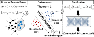
Figure 2: Proposed framework.

Definition 2 (structural consistency of a tensor).

A tensor-valued estimator $T^{(n)}$ of order-$3$ is linearly structurally consistent with high probability, if there exists an affine map $\mathcal{L}\,:\,\mathbb{R}^{M}\rightarrow\mathbb{R}$ (or hyperplane) that separates the underlying features associated with connected pairs from those associated with disconnected pairs w.h.p., that is,

$$\begin{array}[]{cccl}\mathbb{P}\left(\mathcal{L}(\mathcal{T}^{(n)}_{ij})>0\right)&\overset{n\rightarrow\infty}{\longrightarrow}&1,&\mbox{ if }ij\mbox{ is connected,}\\ &&&\\ \mathbb{P}\left(\mathcal{L}(\mathcal{T}^{(n)}_{ij})\leq 0\right)&\overset{n\rightarrow\infty}{\longrightarrow}&1,&\mbox{ if }ij\mbox{ is disconnected}\end{array}.$$ (7)

As an example, the estimator $T^{(n)}$ whose $ij^{\text{th}}$ entry of the tensor output $\mathcal{T}^{(n)}$ is defined as

$$\mathcal{T}^{(n)}_{ij}\overset{\Delta}{=}\left(\left[\widehat{R}_{D}(n)\right]_{ij},\left[\widehat{R}_{D+1}(n)\right]_{ij},\ldots,\left[\widehat{R}_{L}(n)\right]_{ij}\right)$$

corresponds to an order-$3$ tensor-valued estimator. As we will show in the next section, if $D\leq 1$ and $L\geq 3$, then this estimator is linearly structurally consistent w.h.p.

Features Separability & Explainability

This section provides the explainability results underlying the ML approach for graph learning considered in this work.

Assumption 1.

Let $\mathcal{E}^{(n)}:=\left\{E^{(n)}_{1},E^{(n)}_{2},\ldots,E^{(n)}_{M}\right\}$ be a family of matrix-valued estimators such that for some $\mathbf{w}:=\left(w_{1},w_{2},\ldots,w_{M}\right)\in\mathbb{R}^{M}$ with $\mathbf{w}\neq 0$, the linear combination $E^{(n)}(\mathbf{w})=\sum_{\ell=1}^{M}w_{\ell}E^{(n)}_{\ell}$ is a structurally consistent w.h.p. matrix-valued estimator for the dynamics (1).

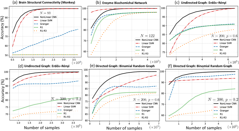
Figure 3: (a)-(f) Structure estimation performance: we plot the estimators’ accuracy as a function of the number of samples. Plots (a)-(b) refer to real-world networks; (c)-(d) refer to undirected graphs (realization of an Erdős–Rényi model); and plots (e)-(f) refer to directed graphs (realization of a binomial random graph). We assume that we can only observe $\left|S\right|=20$ nodes.

Lemma 1.

For each pair $ij$, with $i\neq j$, define the associated feature vector as,

$$\mathcal{T}^{(n)}_{ij}:=\left(\left[E^{(n)}_{1}\right]_{ij},\left[E^{(n)}_{2}\right]_{ij},\ldots,\left[E^{(n)}_{M}\right]_{ij}\right)\in\mathbb{R}^{M}.$$ (8)

Then, under Assumption 1, the tensor-valued estimator $T^{(n)}$ is linearly structurally consistent w.h.p., or equivalently, the set of features $\left\{\mathcal{T}^{(n)}_{ij}\right\}_{i\neq j}\subset\mathbb{R}^{M}$ is consistently linearly separable w.h.p.

Proof.

Since $E^{(n)}(\mathbf{w})=\sum_{\ell=1}^{M}w_{\ell}E^{(n)}_{\ell}$ is structurally consistent w.h.p. for some $\mathbf{w}\in\mathbb{R}^{M}$, then there exists a threshold $\tau_{\mathbf{w}}$ so that $\left[E^{(n)}(\mathbf{w})\right]_{ij}>\tau_{\mathbf{w}}$ across connected pairs $ij$ and $\left[E^{(n)}(\mathbf{w})\right]_{ij}<\tau_{\mathbf{w}}$, otherwise. Therefore, the affine map $\mathcal{L}_{\mathbf{w}}(\mathbf{x})=\mathbf{x}\cdot\mathbf{w}-\tau_{\mathbf{w}}$ consistently separates the set of features $\left\{\mathcal{T}^{(n)}_{ij}\right\}_{ij}$ w.h.p. Indeed,

$$\mathcal{L}_{\mathbf{w}}(\mathcal{T}^{(n)}_{ij})=\mathcal{T}^{(n)}_{ij}\cdot\mathbf{w}-\tau_{\mathbf{w}}=\left[E(\mathbf{w})\right]_{ij}-\tau_{\mathbf{w}}>0$$ (9)

for a connected pair $ij$ or

$$\mathcal{L}_{\mathbf{w}}(\mathcal{T}^{(n)}_{ij})=\left[E^{(n)}(\mathbf{w})\right]_{ij}-\tau_{\mathbf{w}}<0,$$ (10)

otherwise. In other words, the hyperplane characterized by the linear map $\mathcal{L}_{\mathbf{w}}\,:\,\mathbb{R}^{M}\longrightarrow\mathbb{R}$ separates consistently the pairs $ij$ for all $i\neq j$, w.h.p. ∎

Theorem 1.

For each pair $ij$, with $i\neq j$, define the associated feature vector as,

$$\mathcal{T}_{ij}^{(n)}:=\left(\left[\widehat{R}_{D}(n)\right]_{ij},\left[\widehat{R}_{D+1}(n)\right]_{ij},\ldots,\left[\widehat{R}_{L}(n)\right]_{ij}\right),$$

with $D\leq 1$ and $L\geq 3$, and assume that the interaction matrix $A$ underlying the dynamics (1) is symmetric and the covariance matrix of the noise process $\left(\mathbf{x}(n)\right)_{n\in\mathbb{N}}$ is given by $\Sigma_{x}:=\sigma^{2}I_{N}$, for some $\sigma>0$. Then, the set $\left\{\mathcal{T}_{ij}^{(n)}\right\}_{i\neq j}\subset\mathbb{R}^{M}$ is consistently linearly separable w.h.p.

Proof.

Define the vector $\mathbf{w}\in\left\{-1,0,1\right\}^{M}$ so that $E^{(n)}(\mathbf{w})=\widehat{R}_{1}(n)-\widehat{R}_{3}(n)$, which is possible since $D\leq 1$ and $L\geq 3$. According to Theorem 1 in (Chen, Wang, and Shen 2022), $E^{(n)}(\mathbf{w})=\widehat{R}_{1}(n)-\widehat{R}_{3}(n)$ is structurally consistent w.h.p. and the result now follows from the previous Lemma 1. ∎

Remark 2 (Locality of the structural estimation).

Note that, to compute the feature $\mathcal{T}^{(n)}_{ij}$ associated with each pair $ij$ defined in Theorem $1$, we need only the time series $\left\{y_{i}(\ell),y_{j}(\ell)\right\}_{\ell=0}^{n}$ associated with the pair $ij$ as

$$\mathcal{T}_{ij}^{(n)}:=\frac{1}{n}\sum_{\ell=0}^{n-1}\left(y_{i}(\ell+D)y_{j}(\ell),\ldots,y_{i}(\ell+M)y_{j}(\ell)\right),$$

which only involves information related to nodes $i$ and $j$. As such, it is possible to reconstruct the connectivity pattern in a pairwise manner. This is a special property that results from the fact that each lag-moment, or covariance matrix, in the feature vector can be locally estimated. Observe that the majority of the matrix-valued estimators does not exhibit this locality property. For example, to reconstruct the $ij^{\text{th}}$ entry of the Precision matrix $\left(\widehat{R}_{0}(n)\right)^{-1}$, one needs to know the whole matrix $\widehat{R}_{0}(n)$ (or a large portion around the pair $ij$ thereof). This has the drawback of implying the observation of a large set of nodes (or of the whole network) just to estimate the corresponding entry $ij$ of the Precision matrix.

Now, given a matrix-valued estimator $F^{(n)}$, define its identifiability gap as (Matta, Santos, and Sayed 2022)

$$\Gamma\left(F^{(n)}\right)\overset{\Delta}{=}\min_{ij\,:\,A_{ij}\neq 0}\mathcal{F}^{(n)}_{ij}-\max_{ij\,:\,A_{ij}=0}\mathcal{F}_{ij}^{(n)},$$ (11)

i.e., the gap between the smallest entry of $\mathcal{F}_{ij}^{(n)}$ across connected pairs and the largest entry of $\mathcal{F}^{(n)}_{ij}$ over disconnected pairs. An estimator $F^{(n)}$ is structurally consistent w.h.p. if and only if $\Gamma\left(F^{(n)}\right)>0$ w.h.p., or in other words, if and only if connected pairs are separated from disconnected pairs, in view of the entries of the matrix $\mathcal{F}^{(n)}$, for $n$ large enough. This statistical metric is a relevant parameter regarding the hardness of the classification. The larger the identifiability gap, the easier the classification via thresholding of the entries of the matrix $\mathcal{F}^{(n)}$ tends to be.

Similarly, define the identifiability gap $\Gamma\left(T^{(n)}\right)$ associated with a tensor-valued estimator $T^{(n)}$ as the maximum distance among all parallel hyperplanes that consistently separate the features, as in Fig. 2. For example, the SVM algorithm is designed to find these margins. More concretely,

$$\Gamma\left(T^{(n)}\right)\overset{\Delta}{=}\max\limits_{\left(\mathbf{w},\tau_{1}\right),\left(\mathbf{w},\tau_{2}\right)\in\mathcal{H}}\frac{\left|\tau_{1}-\tau_{2}\right|}{\left|\left|\mathbf{w}\right|\right|},$$ (12)

where $\mathcal{H}$ indexes the set of linear maps that consistently separate the features: $\left(\mathbf{w},\tau\right)\in\mathcal{H}$ if and only if the linear map $\mathcal{L}_{\mathbf{w},\tau}(\mathbf{x}):=\mathbf{w}\cdot\mathbf{x}-\tau$ consistently separates the features.

Lemma 2.

Let $T^{(n)}$ be a tensor-valued estimator whose underlying features at each pair $ij$ are defined as

$$\mathcal{T}^{(n)}_{ij}:=\left(\left[E^{(n)}_{1}\right]_{ij},\left[E^{(n)}_{2}\right]_{ij},\ldots,\left[E^{(n)}_{M}\right]_{ij}\right)\in\mathbb{R}^{M},$$ (13)

with identifiability gap $\Gamma_{E}^{(n)}\overset{\Delta}{=}\Gamma\left(T^{(n)}\right)$. Let $\widehat{A}^{(n)}$ be a matrix-valued estimator with identifiability gap $\Gamma_{A}^{(n)}\overset{\Delta}{=}\Gamma\left(\widehat{A}^{(n)}\right)$. If both $\widehat{A}^{(n)}$ and $T^{(n)}$ are (linearly) structurally consistent w.h.p., then the tensor-valued estimator $\widetilde{T}^{(n)}$ defined via the augmented features

$$\widetilde{\mathcal{T}}^{(n)}_{ij}:=\left(\left[\widehat{A}^{(n)}\right]_{ij},\left[E^{(n)}_{1}\right]_{ij},\ldots,\left[E^{(n)}_{M}\right]_{ij}\right)\in\mathbb{R}^{M},$$ (14)

exhibits an identifiability gap obeying $\Gamma\left(\widetilde{T}^{(n)}\right)\geq\left|\left|\Gamma^{(n)}\right|\right|_{2}$ w.h.p., with $\Gamma^{(n)}\overset{\Delta}{=}\left(\Gamma_{A}^{(n)},\Gamma_{E}^{(n)}\right)$.

Lemma 2 asserts that, if further matrix-valued structurally consistent estimators are incorporated into the feature vector, the identifiability gap increases.

Proof.

Let ${\sf Cv}\left(\mathcal{S}\right)$ denote the convex hull of a set $\mathcal{S}\subset\mathbb{R}^{M}$, i.e., the smallest convex set containing $\mathcal{S}$ (Hiriart-Urruty and Lemaréchal 2001). Define $\widetilde{\mathcal{C}}\overset{\Delta}{=}\left\{\widetilde{\mathcal{T}}^{(n)}_{ij}\right\}_{ij\,:\,A_{ij}\neq 0}$ as the set of augmented features associated with connected pairs and $\widetilde{\mathcal{D}}\overset{\Delta}{=}\left\{\widetilde{\mathcal{T}}^{(n)}_{ij}\right\}_{ij\,:\,A_{ij}=0}$ associated with disconnected pairs. Similarly, define $\mathcal{C}\overset{\Delta}{=}\left\{\mathcal{T}^{(n)}_{ij}\right\}_{ij\,:\,A_{ij}\neq 0}$ and $\mathcal{D}\overset{\Delta}{=}\left\{\mathcal{T}^{(n)}_{ij}\right\}_{ij\,:\,A_{ij}=0}$. Let $R$ be the smallest entry of $\widehat{A}^{(n)}$ across connected pairs and $r$ be the greatest entry of $\widehat{A}^{(n)}$ across disconnected pairs and note that $r<R$ w.h.p, since $\widehat{A}^{(n)}$ is structurally consistent w.h.p. We have that

$$\begin{array}[]{ccl}\Gamma\left(\widetilde{T}^{(n)}\right)^{2}\!\!\!\!&\overset{(a)}{=}&\!\!\!\!{\sf d}\left({\sf Cv}\left(\widetilde{\mathcal{C}}\right),{\sf Cv}\left(\widetilde{\mathcal{D}}\right)\right)^{2}\\ \!\!\!\!&\overset{(b)}{\geq}&\!\!\!\!{\sf d}\left({\sf Cv}\left(\mathcal{C}\times\!\!\left.\left[R,\infty\right.\right)\right),{\sf Cv}\left(\mathcal{D}\times\!\!\left.\left(-\infty,r\right.\right]\right)\right)^{2}\\ \!\!\!\!&\overset{(c)}{\geq}&\!\!\!\!{\sf d}\left({\sf Cv}\left(\mathcal{C}\right)\times\!\!\left.\left[R,\infty\right.\right),{\sf Cv}\left(\mathcal{D}\right)\times\!\!\left.\left(-\infty,r\right.\right]\right)^{2}\\ \!\!\!\!&\overset{(d)}{=}&\!\!\!\!{\sf d}\left({\sf Cv}\left(\mathcal{C}\right),{\sf Cv}\left(\mathcal{D}\right)\right)^{2}+(R-r)^{2}\\ \!\!\!\!&=&\!\!\!\!\left(\Gamma^{(n)}_{E}\right)^{2}+\left(\Gamma^{(n)}_{A}\right)^{2}=\left|\left|\Gamma^{(n)}\right|\right|_{2}^{2}\end{array}$$

where for two subsets $\mathcal{X},\mathcal{Y}\subset{R}^{M}$, $d\left(\mathcal{X},\mathcal{Y}\right)$ is the distance

$${\sf d}\left(\mathcal{X},\mathcal{Y}\right)\overset{\Delta}{=}\inf_{x\in\mathcal{X},y\in\mathcal{Y}}\left|\left|x-y\right|\right|_{2};$$ (15)

the first identity $(a)$ conforms to an alternative dual characterization for the identifiability gap (refer to Theorem $13$ in (Dax 2006)); $(b)$ holds in view of the inclusions $\widetilde{\mathcal{C}}\subset\mathcal{C}\times\left.\left[R,\infty\right.\right)$ and $\widetilde{\mathcal{D}}\subset\mathcal{D}\times\left.\left(-\infty,r\right.\right]$; $(c)$ holds since $\mathcal{C}\subset{\sf Cv}\left(\mathcal{C}\right)$ and $\mathcal{D}\subset{\sf Cv}\left(\mathcal{D}\right)$ and the fact that the convex hull commutes with the Cartesian product over convex sets (Hiriart-Urruty and Lemaréchal 2001); the identity $(d)$ is straightforward from the definition of the distance ${\sf d}(\cdot,\cdot)$. ∎

Methodology

In order to stratify the pairs of nodes into connected or disconnected from the observed time series, we address the linear separability property of the covariance-based features $\left\{\mathcal{T}^{(n)}_{ij}\right\}_{ij}$ established in Theorem $1$, by studying the performance of trained classifiers, in particular, linear Support Vector Machines (SVMs) and Convolutional Neural Networks (CNNs). The training set is given by

$${\sf Tr}^{(n)}\overset{\Delta}{=}\left\{\left(\overline{\mathcal{T}}^{(n)}_{ij},\mathbf{1}_{\left\{A_{ij}\neq 0\right\}}\right)\right\}_{i\neq j}$$ (16)

where we have introduced the normalized feature vectors

$$\overline{\mathcal{T}}^{(n)}_{ij}:=\frac{\mathcal{T}^{(n)}_{ij}}{\max_{i\neq j}\left|\left|\mathcal{T}^{(n)}_{ij}\right|\right|_{\infty}},$$ (17)

with the unnormalized features given by,

$$\mathcal{T}_{ij}^{(n)}\overset{\Delta}{=}\left(\left[\widehat{R}_{-100}(n)\right]_{ij},\left[\widehat{R}_{-99}(n)\right]_{ij},\ldots,\left[\widehat{R}_{100}(n)\right]_{ij}\right).$$

In other words, for training, we provide a normalized feature $\overline{\mathcal{T}}^{(n)}_{ij}$ associated with the pair $ij$ as input to a classifier and the output should be the ground truth $1_{\left\{A_{ij}\neq 0\right\}}$.

The normalization in the training set is motivated by the following observation. With infinitely many samples,

$$\mathcal{T}^{\infty}_{ij}=\sigma^{2}\left(\left[\overline{R}_{D}\right]_{ij},\left[\overline{R}_{D+1}\right]_{ij},\ldots,\left[\overline{R}_{M}\right]_{ij}\right)$$ (18)

where $\overline{R}_{k}$ is the $k$-lag covariance matrix (equation (2)) of the normalized process $\left(\mathbf{y}(n)/\sigma\right)_{n\in\mathbb{N}}$, i.e., the process whose noise is normalized to unit variance. With the proposed normalization in equation (17), the multiplicative factor $\sigma^{2}$ is cancelled out, which decreases the role played by the noise-level in the performance of the trained CNNs. Furthermore, this normalization renders the generalization performance of the trained CNNs robust across structurally distinct graphs.

To generate the matrix $A$ to obtain the time series data $\left\{\mathbf{y}(\ell)\right\}_{\ell=0}^{n}$, given a graph $G$, the following procedure was considered. Let $G$ be a given graph without self-loops, i.e., $G_{ii}=0$ for all $i$. Define the interaction matrix $A$ as

$$\left\{\begin{array}[]{ccll}A_{ij}&=&\alpha_{1}\frac{G_{ij}}{d_{\max}(G)},&\mbox{ for }i\neq j\\ A_{ii}&=&\alpha-\sum_{k\neq i}A_{ik},&\mbox{ for all }i\end{array},\right.$$ (19)

where $d_{\max}(G)$ is the maximum in-flow degree of the underlying graph $G$ and $0<\alpha_{1}\leq\alpha<1$ are some constants. In other words, the rows of $A$ sum to $\alpha<1$ and its support is given by $G$. This is often cast as the Laplacian rule (Sayed 2014). This interaction matrix renders the networked dynamical system (1) stable and with a support graph of interactions given by $G$. To generate the support graph $G$, we considered the realization of random graph models as Erdős–Rényi for undirected graphs, binomial random graphs for directed graphs, and real-world networks.

We train the classifiers over one realization of a random graph model with $p=0.5$ and $N=100$ and apply them to distinct networks, including real-world ones, where $p$ is the probability of edge or arrow drawing in the random graph model and $N$ is the number of nodes. Throughout, we assume that we can only observe the time series data from $\left|S\right|=20$ nodes, that is, we assume $S=\left\{1,2,\ldots,20\right\}$.

Simulation Results

In the numerical results considered, we define accuracy as the number of directed pairs correctly classified over the total number of directed pairs in the underlying graph. We consider $1000$ Monte Carlo runs across all plots.

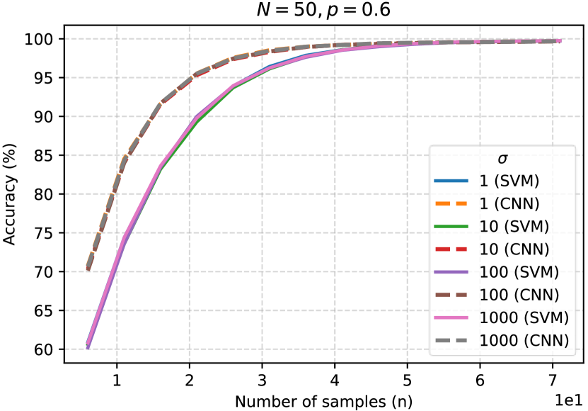
(a)

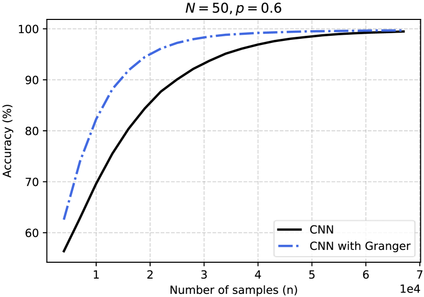
(b)

Figure 4: (a) depicts the robustness against the noise variance for both the CNN and the SVM; and (b) considers the inclusion of the Granger estimator in the feature vector.

Fig. 3 $(a)-(f)$ depict the sample-complexity performance of the estimators across structurally distinct networks, considering: $i$) Granger under partial observability $\left[\widehat{R}_{1}(n)\right]_{\mathcal{S}}\left(\left[\widehat{R}_{0}(n)\right]_{\mathcal{S}}\right)^{-1}$ that is provably structurally consistent (Santos, Matta, and Sayed 2020; Matta, Santos, and Sayed 2020) for distinct regimes of network connectivity; $ii$) The one-lag estimator $\widehat{R}_{1}(n)$, which is also consistent for several network connectivity regimes (Matta, Santos, and Sayed 2022); $iii$) the $\widehat{R}_{1}(n)-\widehat{R}_{3}(n)$ that is structurally consistent (Chen, Wang, and Shen 2022); $iv$) the linear SVM; and $v$) the trained CNNs. For classification, we apply Gaussian mixture over the sorted entries of the matrix-valued estimators in order to stratify the connected and disconnected pairs. Our results show the overall superiority in performance for the CNN-based classifier. Figs. 3 $(a)-(b)$ refer to real-world networks obtained from the database (Rossi and Ahmed 2015), with $(a)$ for a Brain structural connectivity matrix of a monkey and $(b)$ for an enzyme biochemical network; $(c)-(d)$ refer to symmetric regimes where the underlying support graph of the networked dynamical system is undirected; and $(e)-(f)$ refer to directed graph regimes. $N$ and $p$ stand for the number of nodes and probability of edge/arrow drawing in the random graph models. It should be remarked that while the CNN is trained over a synthetic network, namely, a particular realization of an Erdős–Rényi (for undirected networks) random graph model with $p=0.5$ and $N=100$, it generalizes well over real-world networks as demonstrated in Figs. 3 $(a)-(b)$.

Fig. 4(a) illustrates the robustness of both the trained CNNs and the linear SVMs against distinct noise-level regimes. The CNNs and SVMs are trained with a noise variance of $\sigma^{2}=0.5$, but generalize well over an extended range of noise variance. Fig. 4(a) shows that the performance of these classifiers is not sensitive to the variance of the input noise in the dynamics (1). Fig. 4(b) shows the gain in performance when the Granger estimator is included in the feature vector. In particular, when we include in the feature vector

$$\mathcal{T}_{ij}^{(n)}\overset{\Delta}{=}\left(\left[\widehat{A}_{\mathcal{S}}\right]_{ij},\left[\widehat{R}_{-100}(n)\right]_{ij},\ldots,\left[\widehat{R}_{100}(n)\right]_{ij}\right)$$

the additional component $\widehat{A}_{\mathcal{S}}\overset{\Delta}{=}\left[\widehat{R}_{1}(n)\right]_{\mathcal{S}}\left(\left[\widehat{R}_{0}(n)\right]_{\mathcal{S}}\right)^{-1}$ that is the Granger under partial observability, with only $\left|S\right|=20$ nodes observed. This is consistent with Lemma 2, motivating the search for feature vectors built on other matrix-valued structurally consistent estimators. It motivates the following causal inference paradigm: $i$) characterize matrix-valued structurally consistent estimators; $ii$) define feature vectors that collect these consistent estimators; $iii$) use these new features to train classifiers like a CNN.

Concluding Remarks

This paper considered the problem of determining the graph that captures the fundamental dependencies among time series of data. These time series are indexed as nodes in linear stochastic networked dynamical systems. Only the time series of some nodes are observed (partial observability). We proposed a novel feature-based paradigm and proved that the features were consistently linearly separable. With this separability property, our features can be used as an input to a variety of machine learning pipelines in order to design new state-of-the-art algorithms for causal inference of linear networked dynamical systems. In particular, CNNs trained over this set of features exhibited remarkable sample-complexity performance, significantly reducing the number of samples required to reach a certain level of accuracy, as compared with other state-of-the-art estimators, which require a much larger number of samples. Simulation results show the superiority of the CNN-based approach. It was further shown that the inclusion of structurally consistent matrix-valued estimators in the feature vectors increases the performance of structure identification. This motivates further study of new structurally consistent matrix-valued estimators as building blocks for feature vectors or tensor-valued estimators.

References

- Adams, Hansen, and Zhang (2021) Adams, J.; Hansen, N. R.; and Zhang, K. 2021. Identification of Partially Observed Causal Models: Graphical Conditions for the Linear Non-Gaussian and Heterogeneous Cases. In Advances in Neural Information Processing Systems 34 pre-proceedings (NeurIPS 2021), NeurIPS ’21.
- Anandkumar et al. (2013) Anandkumar, A.; Hsu, D.; Javanmard, A.; and Kakade, S. 2013. Learning Linear Bayesian Networks with Latent Variables. In Proceedings of the 30th International Conference on Machine Learning, volume 28 of Proceedings of Machine Learning Research, 249–257. Atlanta, Georgia, USA: PMLR.
- Anandkumar et al. (2012) Anandkumar, A.; Tan, V. Y. F.; Huang, F.; and Willsky, A. S. 2012. High-dimensional Gaussian Graphical Model Selection: Walk Summability and Local Separation Criterion. J. Mach. Learn. Res., 13(1): 2293–2337.
- Anandkumar and Valluvan (2013) Anandkumar, A.; and Valluvan, R. 2013. Learning loopy graphical models with latent variables: Efficient methods and guarantees. Ann. Statist., 41(2): 401–435.
- Barrat, Barthélemy, and Vespignani (2012) Barrat, A.; Barthélemy, M.; and Vespignani, A. 2012. Dynamical Processes on Complex Networks. London, UK: Cambridge University Press. ISBN 9781107626256.
- Bazzi et al. (2016) Bazzi, M.; Porter, M. A.; Williams, S.; McDonald, M.; Fenn, D. J.; and Howison, S. D. 2016. Community Detection in Temporal Multilayer Networks, with an Application to Correlation Networks. Multiscale Modeling & Simulation, 14(1): 1–41.
- Bogdanov, Mossel, and Vadhan (2008) Bogdanov, A.; Mossel, E.; and Vadhan, S. 2008. The Complexity of Distinguishing Markov Random Fields. In Approximation, Randomization and Combinatorial Optimization. Algorithms and Techniques, 331–342. Berlin, Heidelberg: Springer Berlin Heidelberg. ISBN 978-3-540-85363-3.
- Braunstein et al. (2016) Braunstein, A.; Dall’Asta, L.; Semerjian, G.; and Zdeborová, L. 2016. Network dismantling. Proceedings of the National Academy of Sciences, 113(44): 12368–12373.
- Bresler, Gamarnik, and Shah (2014) Bresler, G.; Gamarnik, D.; and Shah, D. 2014. Hardness of Parameter Estimation in Graphical Models. In Proceedings of the 27th International Conference on Neural Information Processing Systems - Volume 1, NIPS’14, 1062–1070. Cambridge, MA, USA: MIT Press.
- Chandrasekaran, Parrilo, and Willsky (2012) Chandrasekaran, V.; Parrilo, P. A.; and Willsky, A. S. 2012. Latent variable graphical model selection via convex optimization. The Annals of Statistics, 40(4): 1935–1967.
- Chen, Wang, and Shen (2022) Chen, Y.; Wang, Z.; and Shen, X. 2022. An Unbiased Symmetric Matrix Estimator for Topology Inference under Partial Observability. IEEE Signal Processing Letters, 29(02): 1257–1261.
- Chickering (2003) Chickering, D. M. 2003. Optimal Structure Identification with Greedy Search. J. Mach. Learn. Res., 3(null): 507–554.
- Ching and Tam (2017) Ching, E. S. C.; and Tam, H. C. 2017. Reconstructing links in directed networks from noisy dynamics. Phys. Rev. E, 95: 010301.
- Chow and Liu (1968) Chow, C.; and Liu, C. 1968. Approximating discrete probability distributions with dependence trees. IEEE Transactions on Information Theory, 14(3): 462–467.
- Colombo et al. (2012) Colombo, D.; Maathuis, M. H.; Kalisch, M.; and Richardson, T. S. 2012. Learning High-dimensional Directed Acyclic Graphs with Latent and Selection Variables. The Annals of Statistics, 40(1): 294–321.
- Dax (2006) Dax, A. 2006. The distance between two convex sets. Linear Algebra and its Applications, 416(1): 184–213. Special Issue devoted to the Haifa 2005 conference on matrix theory.
- Douw et al. (2010) Douw, L.; De Groot, M.; Dellen, E.; Heimans, J.; Ronner, H.; Stam, C.; and Reijneveld, J. 2010. ‘Functional Connectivity’ is a Sensitive Predictor of Epilepsy Diagnosis after the First Seizure. PloS one, 5.
- Fenn et al. (2009) Fenn, D. J.; Porter, M. A.; McDonald, M.; Williams, S.; Johnson, N. F.; and Jones, N. S. 2009. Dynamic communities in multichannel data: An application to the foreign exchange market during the 2007–2008 credit crisis. Chaos: An Interdisciplinary Journal of Nonlinear Science, 19(3): 033119.
- Fenn et al. (2012) Fenn, D. J.; Porter, M. A.; Mucha, P. J.; McDonald, M.; Williams, S.; Johnson, N. F.; and Jones, N. S. 2012. Dynamical clustering of exchange rates. Quantitative Finance, 12(10): 1493–1520.
- Ganesh, Massoulié, and Towsley (2005) Ganesh, A.; Massoulié, L.; and Towsley, D. 2005. The effect of network topology on the spread of epidemics. In Proceedings IEEE 24th Annual Joint Conference of the IEEE Computer and Communications Societies., volume 2, 1455–1466.
- Geiger et al. (2015) Geiger, P.; Zhang, K.; Schölkopf, B.; Gong, M.; and Janzing, D. 2015. Causal Inference by Identification of Vector Autoregressive Processes with Hidden Components. In Proc. International Conference on Machine Learning, volume 37, 1917–1925.
- Granger (1969) Granger, C. W. J. 1969. Investigating Causal Relations by Econometric Models and Cross-spectral Methods. Econometrica, 37(3): 424–438.
- Hammersley and Clifford (2021) Hammersley, J. M.; and Clifford, P. 2021. Markov fields on finite graphs and lattices. University of Oxford.
- Hiriart-Urruty and Lemaréchal (2001) Hiriart-Urruty, J.-B.; and Lemaréchal, C. 2001. Fundamentals of Convex Analysis. Grundlehren Text Editions. Springer-Verlag Berlin Heidelberg. ISBN 978-3-540-42205-1.
- Jalali and Sanghavi (2012) Jalali, A.; and Sanghavi, S. 2012. Learning the Dependence Graph of Time Series with Latent Factors. In Proceedings of the 29th International Coference on International Conference on Machine Learning, ICML’12, 619–626. Madison, WI, USA: Omnipress. ISBN 9781450312851.
- Kivits and Hof (2022) Kivits, E.; and Hof, P. M. V. d. 2022. Identification of diffusively coupled linear networks through structured polynomial models. IEEE Transactions on Automatic Control, 1–16.
- Lahmanovich and James (1976) Lahmanovich, A.; and James, A. Y. 1976. A Deterministic Model for Gonorrhea in a Nonhomogeneous Population. Mathematical Biosciences, 28: 221–236.
- Lehnertz, Bröhl, and Rings (2020) Lehnertz, K.; Bröhl, T.; and Rings, T. 2020. The Human Organism as an Integrated Interaction Network: Recent Conceptual and Methodological Challenges. Frontiers in Physiology, 11.
- Liégeois et al. (2020) Liégeois, R.; Santos, A.; Matta, V.; Van De Ville, D.; and Sayed, A. H. 2020. Revisiting correlation-based functional connectivity and its relationship with structural connectivity. Network Neuroscience, 4(4): 1235–1251.
- Liggett (2005) Liggett, T. 2005. Interacting Particle Systems. Springer-Verlag Berlin Heidelberg, first edition. ISBN 978-3-540-26962-5.
- Lim et al. (2015) Lim, N.; d’Alché Buc, F.; Auliac, C.; and Michailidis, G. 2015. Operator-valued kernel-based vector autoregressive models for network inference. Machine Learning, 99(3): 489–513.
- Mastakouri, Schölkopf, and Janzing (2021) Mastakouri, A. A.; Schölkopf, B.; and Janzing, D. 2021. Necessary and sufficient conditions for causal feature selection in time series with latent common causes. In Proceedings of the 38th International Conference on Machine Learning, volume 139 of Proceedings of Machine Learning Research, 7502–7511. PMLR.
- Mateos et al. (2019) Mateos, G.; Segarra, S.; Marques, A. G.; and Ribeiro, A. 2019. Connecting the Dots: Identifying Network Structure via Graph Signal Processing. IEEE Signal Processing Magazine, 36(3): 16–43.
- Materassi and Salapaka (2012a) Materassi, D.; and Salapaka, M. V. 2012a. Network reconstruction of dynamical polytrees with unobserved nodes. In Proc. IEEE Conference on Decision and Control (CDC), 4629–4634. Maui, Hawaii.
- Materassi and Salapaka (2012b) Materassi, D.; and Salapaka, M. V. 2012b. On the problem of reconstructing an unknown topology via locality properties of the Wiener filter. IEEE Transactions on Automatic Control, 57(7): 1765–1777.
- Materassi and Salapaka (2015) Materassi, D.; and Salapaka, M. V. 2015. Identification of network components in presence of unobserved nodes. In Proc. IEEE Conference on Decision and Control (CDC), 1563–1568. Osaka, Japan.
- Matta, Santos, and Sayed (2020) Matta, V.; Santos, A.; and Sayed, A. H. 2020. Graph Learning under Partial Observability. Proceedings of the IEEE, 108: 2049 – 2066.
- Matta, Santos, and Sayed (2022) Matta, V.; Santos, A.; and Sayed, A. H. 2022. Graph Learning over Partially Observed Diffusion Networks: Role of Degree Concentration. IEEE Open Journal of Signal Processing, 335–371.
- Mauroy and Goncalves (2016) Mauroy, A.; and Goncalves, J. 2016. Linear identification of nonlinear systems: A lifting technique based on the Koopman operator. In 2016 IEEE 55th Conference on Decision and Control (CDC), 6500–6505. Las Vegas, USA.
- Mei and Moura (2017) Mei, J.; and Moura, J. M. F. 2017. Signal Processing on Graphs: Causal Modeling of Unstructured Data. IEEE Transactions on Signal Processing, 65(8): 2077–2092.
- Mei and Moura (2018) Mei, J.; and Moura, J. M. F. 2018. SILVar: Single Index Latent Variable Models. IEEE Transactions on Signal Processing, 66(11): 2790–2803.
- Monajemi et al. (2016) Monajemi, S.; Eftaxias, K.; Sanei, S.; and Ong, S. H. 2016. An Informed Multitask Diffusion Adaptation Approach to Study Tremor in Parkinson’s Disease. IEEE Journal of Selected Topics in Signal Processing, 10(7): 1306–1314.
- Moneta et al. (2009) Moneta, A.; Chlaß, N.; Entner, D.; and Hoyer, P. 2009. Causal Search in Structural Vector Autoregressive Models. In Proceedings of the 12th International Conference on Neural Information Processing Systems (NIPS) Mini-Symposium on Causality in Time Series, 95–118. Vancouver, Canada.
- Napoletani and Sauer (2008) Napoletani, D.; and Sauer, T. D. 2008. Reconstructing the topology of sparsely connected dynamical networks. Physical Review. E, Statistical, Nonlinear, and Soft Matter Physics, 77: 026103.
- Oltra et al. (2021) Oltra, J.; Campabadal Delgado, A.; Segura, B.; Uribe, C.; Marti, M.; Compta, Y.; Valldeoriola, F.; Bargalló, N.; Iranzo, A.; and Junqué, C. 2021. Disrupted functional connectivity in PD with probable RBD and its cognitive correlates. Scientific Reports, 11.
- Pearl (2009) Pearl, J. 2009. Causality. Cambridge University Press, 2 edition.
- Pereira, Ibrahimi, and Montanari (2010) Pereira, J.; Ibrahimi, M.; and Montanari, A. 2010. Learning Networks of Stochastic Differential Equations. In Advances in Neural Information Processing Systems, volume 23. Curran Associates, Inc.
- Porter and Gleeson (2016) Porter, M.; and Gleeson, J. 2016. Dynamical Systems on Networks: A Tutorial. Springer International Publishing. ISBN 9783319266411.
- Ramsey et al. (2016) Ramsey, J.; Glymour, M.; Sanchez-Romero, R.; and Glymour, C. 2016. A million variables and more: the Fast Greedy Equivalence Search algorithm for learning high-dimensional graphical causal models, with an application to functional magnetic resonance images. International Journal of Data Science and Analytics, 3: 121–129.
- Ranasinghe et al. (2014) Ranasinghe, K. G.; Hinkley, L. B.; Beagle, A. J.; Mizuiri, D.; Dowling, A. F.; Honma, S. M.; Finucane, M. M.; Scherling, C.; Miller, B. L.; Nagarajan, S. S.; and Vossel, K. A. 2014. Regional functional connectivity predicts distinct cognitive impairments in Alzheimer’s disease spectrum. NeuroImage: Clinical, 5: 385–395.
- Ren et al. (2019) Ren, X.-L.; Gleinig, N.; Helbing, D.; and Antulov-Fantulin, N. 2019. Generalized network dismantling. Proceedings of the National Academy of Sciences, 116(14): 6554–6559.
- Robert (2003) Robert, P. 2003. Stochastic Networks and Queues. Springer-Verlag. ISBN 978-3-540-00657-2.
- Rossi and Ahmed (2015) Rossi, R. A.; and Ahmed, N. K. 2015. The Network Data Repository with Interactive Graph Analytics and Visualization. In AAAI.
- Sandryhaila and Moura (2013) Sandryhaila, A.; and Moura, J. M. F. 2013. Discrete Signal Processing on Graphs. IEEE Transactions on Signal Processing, 61(7): 1644–1656.
- Santos, Matta, and Sayed (2020) Santos, A.; Matta, V.; and Sayed, A. H. 2020. Local Tomography of Large Networks under the Low-Observability Regime. IEEE Transactions on Information Theory, 66: 587 – 613.
- Santos, Moura, and Xavier (2015) Santos, A.; Moura, J. M. F.; and Xavier, J. 2015. Bi-Virus SIS Epidemics over Networks: Qualitative Analysis. IEEE Transactions on Network Science and Engineering, 2(1): 17–29.
- Sayed (2014) Sayed, A. H. 2014. Adaptation, Learning, and Optimization over Networks. Found. Trends Mach. Learn., 7(4-5): 311–801.
- Segarra et al. (2017) Segarra, S.; Marques, A. G.; Mateos, G.; and Ribeiro, A. 2017. Network Topology Inference from Spectral Templates. IEEE Transactions on Signal and Information Processing over Networks, 3(3): 467–483.
- Segarra, Schaub, and Jadbabaie (2017) Segarra, S.; Schaub, M. T.; and Jadbabaie, A. 2017. Network inference from consensus dynamics. In 2017 IEEE 56th Annual Conference on Decision and Control (CDC), 3212–3217.
- Spirtes and Glymour (1991) Spirtes, P.; and Glymour, C. 1991. An Algorithm for Fast Recovery of Sparse Causal Graphs. Social Science Computer Review, 9(1): 62–72.
- Spirtes, Glymour, and Scheines (2000) Spirtes, P.; Glymour, C.; and Scheines, R. 2000. Causation, Prediction, and Search. MIT press, 2nd edition.
- Spirtes, Meek, and Richardson (1995) Spirtes, P.; Meek, C.; and Richardson, T. 1995. Causal Inference in the Presence of Latent Variables and Selection Bias. In Proceedings of the Eleventh Conference on Uncertainty in Artificial Intelligence, UAI’95, 499–506. San Francisco, CA, USA: Morgan Kaufmann Publishers Inc. ISBN 1558603859.
- Stam et al. (2007) Stam, C.; Jones, B.; Nolte, G.; Breakspear, M.; and Scheltens, P. 2007. Small-World Networks and Functional Connectivity in Alzheimer’s Disease. Cerebral Cortex, 17(1): 92–99.
- van Mierlo et al. (2019) van Mierlo, P.; Höller, Y.; Focke, N. K.; and Vulliemoz, S. 2019. Network Perspectives on Epilepsy Using EEG/MEG Source Connectivity. Frontiers in Neurology, 10.
- Zhao and Wan (2022) Zhao, L.; and Wan, Y. 2022. Identifiability and Estimation of Partially-observed Influence Models. IEEE Control Systems Letters, 1–1.