\xpatchcmd\@thm

Waveform Design for Mutual Interference Mitigation in Automotive Radar

Arindam Bose1, , Bo Tang1, Wenjie Huang, 
Mojtaba Soltanalian2, , Jian Li2
1The authors contributed equally to this work. 2Corresponding authors.This work was supported in part by U.S. National Science Foundation Grants ECCS-1708509 and ECCS-1809225, and an Illinois Discovery Partners Institute (DPI) Seed Award. Parts of this work have been presented at the 2018 IEEE International Conference on Acoustics, Speech and Signal Processing (ICASSP), Calgary, AB, Canada in April, 2018 [1].A. Bose and M. Soltanalian are with the Department of Electrical and Computer Engineering, University of Illinois at Chicago, Chicago, IL 60607 USA (e-mail: abose4, msol@uic.edu).B. Tang is with the Department of Electronic Engineering and Information Science, University of Science and Technology of China, Hefei 230027, China, and also with the Electronic Engineering Institute, Hefei 230000, China (e-mail: tangbo06@gmail.com).W. Huang is with the Department of Electronic Engineering and Information Science, University of Science and Technology of China, Hefei, China.J. Li is with the Department of Electrical and Computer Engineering, University of Florida, Gainesville, FL 32611 USA (e-mail: li@dsp.ufl.edu).
Abstract

The mutual interference between similar radar systems can result in reduced radar sensitivity and increased false alarm rates. To address the synchronous and asynchronous interference mitigation problems in similar radar systems, we first propose herein two slow-time coding schemes to modulate the pulses within a coherent processing interval (CPI) for a single-input-single-output (SISO) scenario. Specifically, the first coding scheme relies on Doppler shifting and the second one is devised based on an optimization approach. We further extend our discussion to the more general case of multiple-input-multiple-output (MIMO) radars and propose an efficient algorithm to design waveforms to mitigate mutual interference in such systems. The proposed coding schemes are computationally efficient in practice and the incorporation of the coding schemes requires only a slight modification of the existing systems. Our numerical examples indicate that the proposed coding schemes can reduce the interference power level in a desired area of the cross-ambiguity function significantly.

Index Terms:
Automotive radar systems, mutual interference mitigation, slow-time coding, code optimization, MIMO.

I Introduction

The radar technology exhibits an unmatched performance in a variety of vehicular applications, owing to its excellent target resolving capabilities in bad weather and low visibility conditions in comparison with visible and infrared imaging techniques [2, 3, 4, 5, 6]. In recent years, due to the benefits of exploiting the millimeter-wave (mm-wave) band such as increased bandwidth, high spatial resolution, smaller size and weight of mm-wave equipment compared to ultrasonic radar and lidar, the mm-wave radars (30-300 GHz) have gained significant popularity not only in automotive radar systems but also in drone radar applications and internet of things (IoT) [7, 8, 9]. For instance, mm-wave radar equipment is much simpler than lidar’s complex mirrors and lasers, but far faster and more accurate than ultrasonic radars, and may use highly directional, high-frequency EM waves to map the surrounding environment [10, 11]. Given the tendency to mass-produce radars for civilian applications (e.g., automotive radars), such systems, however, tend to be quite similar, or even almost identical. The increasing number of similar or identical radar systems increases the probability of mutual interference, which may result in severely reduced radar sensitivity and poor performance quality [12, 13, 14]. Thus it is vitally important to enhance radar signal processing performance in severe mutual interference scenarios [15, 16, 17, 18].

In the literature, the effects of mutual interference and their corresponding methods of mitigation have been discussed widely, e.g., see [19, 20, 21, 22, 23, 24, 25, 26, 27, 28, 29, 30, 31] and the references within. A judicious signal separation method for synchronous and asynchronous interference mitigation is proposed in [19]. The authors in [20] study the impact of radar waveform design and the associated receiver processing on the statistics of radar-to-radar interference and further propose an approach based on pseudo-random cyclic orthogonal sequences (PRCOS), which enable sensors to rapidly learn the interference environment and avoid using frequency overlapping waveforms. An iterative filtering algorithm followed by matched filtering for each radar has been suggested in [21] to suppress the radar-to-radar interferences. Furthermore, in [27], the authors analyzed the mutual interference between frequency-modulated continuous-wave (FMCW) radar systems and proposed several techniques to mitigate the interference problem, including pre-possessing and finite impulse response (FIR) filtering. Contrary to addressing the mutual interference in the receiver side, the authors in [22, 23, 24] investigated the problems between automotive radar systems with different types of transmissions.

In this paper, we address the mutual interference mitigation problem for similar or identical radar systems by using smart transmit waveforms. In particular, we consider a scenario where the manufacturer of the radar systems present in the scene is essentially the same; as a result, the radar parameters such as carrier frequency, slope, and the number of the chirps are assumed to be similar. It is true that in the real world, such a scenario is currently relatively rare. However, as more cars are equipped with radars, this may occur more frequently; something that can be dealt with through future regulations and shared protocols. We further assume that in such radar systems, it is possible to modify the custom waveforms used for transmission on-the-fly. Note that such a scenario can be avoided simply by “orthogonalization” of radar parameters. Designing waveforms, however, can make such a process more optimal, particularly when more than two vehicles are involved. In this sense, this work lays the ground for future sensible solutions in multi-vehicle scenarios.

To this end, we first formulate the problem of waveform designing for a simple single-input-single-output (SISO) case. Particularly, we propose two slow-time coding schemes to reduce the interference power level. Next, we extend our approach to the more general multiple-input-multiple-output (MIMO) scenario. Recently, there has been considerable interest in radar systems employing multiple antennas at both the transmitter and receiver; thus, performing space-time processing on both [32]. Compared with the traditional phased-array radars, a MIMO radar can transmit multiple independent probing waveforms simultaneously, enabling further waveform diversity [33] and enhanced parameter identifiability [34]. Given the pervasive use of MIMO systems, it is of utter importance to design sets of waveforms that will reduce mutual interference between different MIMO automotive radars. The main contributions of this work can be summarized as follows:

  • We begin our study with the SISO case and propose two coding schemes to reduce the interference power level. The first coding scheme aims to shift the Doppler frequency of the interference and separate it from the target in the Doppler region. The second coding scheme aims to minimize the discrete periodic cross-ambiguity function (PCAF) in the desired area.

  • We further formulate the problem of minimizing the discrete PCAF for a general MIMO scenario and propose an efficient cyclic algorithm to design the transmit waveforms.

Note that a distributed and mutually cooperative design protocol can be adopted for the online design of such waveforms in a collaborative manner. The design can also be done offline where the radar codes can be designed and stored in a centralized radar codebook for later usage. The discussion of such design coordination protocols is, however, beyond the scope of this work.

The rest of this paper is organized as follows. In Section II, we discuss the mutual interference for two identical frequency modulated continuous wave (FMCW) radar systems. We propose two coding schemes for the SISO scenario in Section III. Section IV is devoted to waveform design for the more general MIMO scenario. Numerical simulation results are presented in Section V. Finally, Section VI concludes our work.

Notation: We use bold-lowercase and bold-uppercase letters to represent vectors and matrices, respectively. xisubscript𝑥𝑖x_{i} denotes the i𝑖i-th element of the vector 𝐱𝐱\mathbf{x}. The superscripts ()superscript(\cdot)^{*}, ()Tsuperscript𝑇(\cdot)^{T}, and ()Hsuperscript𝐻(\cdot)^{H} represent the conjugate, the transpose, and the Hermitian operators, respectively. The set of complex matrices are denoted by \mathds{C}. {}\Re\{\cdot\} signifies the real part of a complex variable. The psubscript𝑝\ell_{p}-norm is represented by p\|\cdot\|_{p}. The Frobenius norm of the matrix 𝐗𝐗\mathbf{X} is denoted by 𝐗Fsubscriptnorm𝐗𝐹\|\mathbf{X}\|_{F}. 𝐈Nsubscript𝐈𝑁\mathbf{I}_{N} is the identity matrix of size N×N𝑁𝑁N\times N, while 𝟎0\mathbf{0} denotes the all-zero vector/matrix of given size. Diag(𝐱)Diag𝐱\mathrm{Diag}\left(\mathbf{x}\right) denotes a diagonal matrix formed whose diagonal elements are determined by the vector 𝐱𝐱\mathbf{x}. Finally, direct-product\odot represents the Hadamard product of matrices.

II Preliminaries

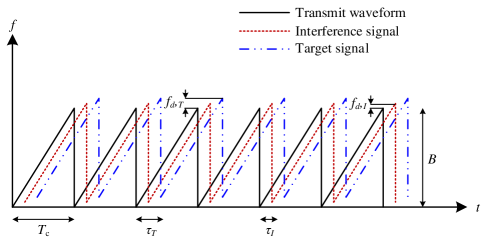
In this section, we start by formulating the problem for a SISO scenario. Consider two identical FMCW radar systems shown in Fig. 1, that are operating within the same frequency band and same B/Tc𝐵subscript𝑇𝑐B/T_{c} ratio where B𝐵B and Tcsubscript𝑇𝑐T_{c} are the FMCW signal bandwidth and chirp time, respectively, as shown in Fig. 1. The transmitted signal can be expressed as

s(t)=n=0C1u(tnTc)𝑠𝑡superscriptsubscript𝑛0𝐶1𝑢𝑡𝑛subscript𝑇𝑐\displaystyle s(t)=\sum_{n=0}^{C-1}{u(t-nT_{c})} (1)

where u(t)=1Tcexp(j(2πfct+πKt2))rect(tTcTc)𝑢𝑡1subscript𝑇𝑐𝑗2𝜋subscript𝑓𝑐𝑡𝜋𝐾superscript𝑡2rect𝑡subscript𝑇𝑐subscript𝑇𝑐u(t)=\frac{1}{\sqrt{T_{c}}}\exp\left(j(2\pi f_{c}t+\pi Kt^{2})\right)\textrm{rect}\left(\frac{t-T_{c}}{T_{c}}\right), fcsubscript𝑓𝑐f_{c} is the carrier frequency, C𝐶C is the number of chirps, K=B/Tc𝐾𝐵subscript𝑇𝑐K=B/T_{c}, and

rect(t)={1,0t1,0,elsewhere.rect𝑡cases10𝑡10elsewhere\displaystyle\textrm{rect}(t)=\left\{\begin{array}[]{ll}1,&0\leq t\leq 1,\\ 0,&~{}\mathrm{elsewhere}.\end{array}\right.
Refer to caption
Refer to caption
Figure 1: Mutual interference between automotive radars: (a) potential source of mutual interference; (b) time-frequency illustration of the transmit waveform, the target signal, and the interference.

When the two radar systems are operating simultaneously, the received signal by one radar includes not only the target reflections but also the interference signal due to the transmission from the other radar system. As a result, we can express the received signal by one radar (e.g., the radar mounted on Car 1 in Fig. 1) as,

r(t)=yT(t)+yI(t)+w(t)𝑟𝑡subscript𝑦𝑇𝑡subscript𝑦𝐼𝑡𝑤𝑡\displaystyle r(t)=y_{T}(t)+y_{I}(t)+w(t) (2)

where yT(t)=αTs(tτT)exp(jπfd,Tt)subscript𝑦𝑇𝑡subscript𝛼𝑇𝑠𝑡subscript𝜏𝑇𝑗𝜋subscript𝑓𝑑𝑇𝑡y_{T}(t)=\alpha_{T}s(t-\tau_{T})\exp(j\pi f_{d,T}t) is the target return, and yI(t)=αIs(tτI)exp(jπfd,It)subscript𝑦𝐼𝑡subscript𝛼𝐼𝑠𝑡subscript𝜏𝐼𝑗𝜋subscript𝑓𝑑𝐼𝑡y_{I}(t)=\alpha_{I}s(t-\tau_{I})\exp(j\pi f_{d,I}t) is the interference signal with αT,αIsubscript𝛼𝑇subscript𝛼𝐼\alpha_{T},\alpha_{I} being the corresponding amplitudes, τTsubscript𝜏𝑇\tau_{T} is the two-way target propagation delay, τIsubscript𝜏𝐼\tau_{I} is the one-way delay associated with the interference, fd,T,fd,Isubscript𝑓𝑑𝑇subscript𝑓𝑑𝐼f_{d,T},f_{d,I} are the corresponding Doppler frequencies, and w(t)𝑤𝑡w(t) is the internal disturbance, including, e.g., the receiver noise.

Typically, FMCW radar systems collect the received signal from N𝑁N consecutive pulses within a coherent processing interval (CPI) for target detection and parameter estimation. The received signal is then conjugately mixed with the transmitted signal to produce a low-frequency intermediate (de-chirped) signal. As a result, the de-chirped version of r(t)𝑟𝑡r(t) for the nthsuperscript𝑛𝑡n^{th} (slow-time) pulse is given by

rdcn(t)superscriptsubscript𝑟𝑑𝑐𝑛𝑡\displaystyle r_{dc}^{n}(t) =αTexp(j2π(fB,Tt+nfd,TTc))absentsubscript𝛼𝑇𝑗2𝜋subscript𝑓𝐵𝑇𝑡𝑛subscript𝑓𝑑𝑇subscript𝑇𝑐\displaystyle=\alpha_{T}\exp(j2\pi(f_{B,T}t+nf_{d,T}T_{c}))
+αIexp(j2π(fB,It+nfd,ITc))+wn(t)subscript𝛼𝐼𝑗2𝜋subscript𝑓𝐵𝐼𝑡𝑛subscript𝑓𝑑𝐼subscript𝑇𝑐superscript𝑤𝑛𝑡\displaystyle~{}+\alpha_{I}\exp(j2\pi(f_{B,I}t+nf_{d,I}T_{c}))+w^{n}(t) (3)

where fB,T=KτT+fd,Tsubscript𝑓𝐵𝑇𝐾subscript𝜏𝑇subscript𝑓𝑑𝑇f_{B,T}=K{\tau_{T}}+f_{d,T}, fB,I=KτI+fd,Isubscript𝑓𝐵𝐼𝐾subscript𝜏𝐼subscript𝑓𝑑𝐼f_{B,I}=K{\tau_{I}}+f_{d,I} are the beat frequencies corresponding to the target and the interference signal, respectively, and to lighten the notations, we absorb the constant phase terms into αTsubscript𝛼𝑇\alpha_{T} and αIsubscript𝛼𝐼\alpha_{I}, and use wn(t)superscript𝑤𝑛𝑡w^{n}(t) to denote the de-chirped noise.

The de-chirped signal is then passed through analog-to-digital converters (ADCs) and the mthsuperscript𝑚𝑡m^{th} (fast-time) digital sample can be expressed as,

r(m,n)𝑟𝑚𝑛\displaystyle r(m,n) =αTexp(j2π(f^B,Tm+f^d,Tn))absentsubscript𝛼𝑇𝑗2𝜋subscript^𝑓𝐵𝑇𝑚subscript^𝑓𝑑𝑇𝑛\displaystyle=\alpha_{T}\exp(j2\pi(\hat{f}_{B,T}m+\hat{f}_{d,T}n))
+αIexp(j2π(f^B,Im+f^d,In))+w(m,n)subscript𝛼𝐼𝑗2𝜋subscript^𝑓𝐵𝐼𝑚subscript^𝑓𝑑𝐼𝑛𝑤𝑚𝑛\displaystyle+\alpha_{I}\exp(j2\pi(\hat{f}_{B,I}m+\hat{f}_{d,I}n))+w(m,n) (4)

where f^B,T=fB,TTs,f^B,I=fB,ITsformulae-sequencesubscript^𝑓𝐵𝑇subscript𝑓𝐵𝑇subscript𝑇𝑠subscript^𝑓𝐵𝐼subscript𝑓𝐵𝐼subscript𝑇𝑠\hat{f}_{B,T}=f_{B,T}T_{s},~{}\hat{f}_{B,I}=f_{B,I}T_{s} are the corresponding normalized beat frequencies, f^d,T=fd,TTc,f^d,I=fd,ITcformulae-sequencesubscript^𝑓𝑑𝑇subscript𝑓𝑑𝑇subscript𝑇𝑐subscript^𝑓𝑑𝐼subscript𝑓𝑑𝐼subscript𝑇𝑐\hat{f}_{d,T}=f_{d,T}T_{c},~{}\hat{f}_{d,I}=f_{d,I}T_{c} are the corresponding normalized Doppler frequencies, and Ts=1/fssubscript𝑇𝑠1subscript𝑓𝑠T_{s}=1/f_{s}, with fssubscript𝑓𝑠f_{s} being the sampling frequency.

Applying 2-D FFT to (II) for m=1,,M𝑚1𝑀m=1,\cdots,M and n=1,,N𝑛1𝑁n=1,\cdots,N, we can obtain the range-Doppler image as,

RD(k,p)RD𝑘𝑝\displaystyle\text{RD}(k,p) =αTDM(f^B,Tk/M)DN(f^d,Tp/N)absentsubscript𝛼𝑇subscript𝐷𝑀subscript^𝑓𝐵𝑇𝑘𝑀subscript𝐷𝑁subscript^𝑓𝑑𝑇𝑝𝑁\displaystyle=\alpha_{T}D_{M}(\hat{f}_{B,T}-k/M)D_{N}(\hat{f}_{d,T}-p/N) (5)
+αIDM(f^B,Ik/M)DN(f^d,Ip/N)+W(k,p)subscript𝛼𝐼subscript𝐷𝑀subscript^𝑓𝐵𝐼𝑘𝑀subscript𝐷𝑁subscript^𝑓𝑑𝐼𝑝𝑁𝑊𝑘𝑝\displaystyle+\alpha_{I}D_{M}(\hat{f}_{B,I}-k/M)D_{N}(\hat{f}_{d,I}-p/N)+W(k,p)

where Dn(x)=sin(nπx)/sin(πx)subscript𝐷𝑛𝑥𝑛𝜋𝑥𝜋𝑥D_{n}(x)=\sin(n\pi x)/\sin(\pi x) is the Dirichlet function and W(k,p)𝑊𝑘𝑝W(k,p) represents the 2-D FFT of noise.

One can observe from (5) that the interference signal will form a sharp peak in the range-Doppler image. In particular, it is worth noting that, although the interference might be attributable to the transmission from the antenna sidelobe of one radar and receiving by the antenna sidelobe of the other, the potential interference level can be significantly higher than the target reflections due to the non-ideal antenna sidelobe characteristic. This is attributable to the one-way propagation characteristic of the interference signal and the direct (without reflection) blast from one’s transmission to the other’s reception [1]. Specifically, according to the radar range-equation, the power of the target returns (i.e., |αT|2superscriptsubscript𝛼𝑇2|\alpha_{T}|^{2}) can be determined by

PT,r=PtGT2λ2σtLt(4π)3RT4,subscript𝑃𝑇𝑟subscript𝑃𝑡superscriptsubscript𝐺𝑇2superscript𝜆2subscript𝜎𝑡subscript𝐿𝑡superscript4𝜋3superscriptsubscript𝑅𝑇4P_{T,r}=\frac{P_{t}G_{T}^{2}\lambda^{2}\sigma_{t}L_{t}}{(4\pi)^{3}R_{T}^{4}}, (6)

where Ptsubscript𝑃𝑡P_{t} is the system transmit power, GTsubscript𝐺𝑇G_{T} is the antenna gain in the target direction, λ=c/fc𝜆𝑐subscript𝑓𝑐\lambda=c/f_{c} is the wavelength, c𝑐c is the light speed, σtsubscript𝜎𝑡\sigma_{t} is the radar cross section (RCS) of the target, Ltsubscript𝐿𝑡L_{t} is the propagation loss, and RTsubscript𝑅𝑇R_{T} denotes the target range. The power of interference (i.e., |αI|2superscriptsubscript𝛼𝐼2|\alpha_{I}|^{2}) is given by

PI,r=PtGt,IGr,Iλ2LI(4π)2RI2,subscript𝑃𝐼𝑟subscript𝑃𝑡subscript𝐺𝑡𝐼subscript𝐺𝑟𝐼superscript𝜆2subscript𝐿𝐼superscript4𝜋2superscriptsubscript𝑅𝐼2P_{I,r}=\frac{P_{t}G_{t,I}G_{r,I}\lambda^{2}L_{I}}{(4\pi)^{2}R_{I}^{2}}, (7)

where we have assumed the two automotive radar systems have the same transmit power, Gt,Isubscript𝐺𝑡𝐼G_{t,I} and Gr,Isubscript𝐺𝑟𝐼G_{r,I} denote the transmit and receive antenna gains associated with the interference, respectively, LIsubscript𝐿𝐼L_{I} denotes the propagation loss, and RIsubscript𝑅𝐼R_{I} is the range between the two radar systems. Thus, considering a target with RCS of 1m21superscriptm21\textrm{m}^{2} and ignoring the propagation loss, we have the power ratio at the receiver input as,

PI,rPT,r=4πRT4Gt,IGr,IGT2RI2.subscript𝑃𝐼𝑟subscript𝑃𝑇𝑟4𝜋superscriptsubscript𝑅𝑇4subscript𝐺𝑡𝐼subscript𝐺𝑟𝐼superscriptsubscript𝐺𝑇2superscriptsubscript𝑅𝐼2\frac{P_{I,r}}{P_{T,r}}=\frac{4\pi R_{T}^{4}G_{t,I}G_{r,I}}{G_{T}^{2}R_{I}^{2}}. (8)

Therefore, the non-negligible interference power will result in serious interference for both automotive radar systems. In the following, we formulate the problem of mutual interference mitigation for a simple SISO scenario and then extend it to the MIMO case.

III SISO Mutual Interference Mitigation
Refer to caption
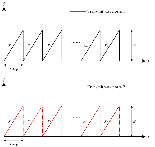
Figure 2: An illustration of the SISO coding scheme for two radar systems operating under same FMCW parameters.

Consider two systems that use N𝑁N periodic consecutive pulses: 𝐱=[x1,x2.,xN]T\mathbf{x}=[x_{1},x_{2}.\cdots,x_{N}]^{T}and 𝐲=[y1,y2.,yN]T\mathbf{y}=[y_{1},y_{2}.\cdots,y_{N}]^{T}, respectively, as depicted in Fig. 2. That is to say, in the nthsuperscript𝑛𝑡n^{th} pulse of a CPI, the first radar system transmits xnu(t)subscript𝑥𝑛𝑢𝑡x_{n}u(t) and the second radar system transmits ynu(t)subscript𝑦𝑛𝑢𝑡y_{n}u(t). Moreover, to keep constant transmit power over the N𝑁N pulses, we constrain the code sequences to be unimodular, i.e., |xn|=|yn|=1,n=1,2,,Nformulae-sequencesubscript𝑥𝑛subscript𝑦𝑛1𝑛12𝑁|x_{n}|=|y_{n}|=1,n=1,2,\cdots,N. With this coding scheme, the mthsuperscript𝑚𝑡m^{th} (fast-time) sample of the nthsuperscript𝑛𝑡n^{th} de-chirped signal is denoted by,

rc(m,n)superscript𝑟𝑐𝑚𝑛\displaystyle r^{c}(m,n) =αTexp(j2π(f^B,Tm+f^d,Tn))absentsubscript𝛼𝑇𝑗2𝜋subscript^𝑓𝐵𝑇𝑚subscript^𝑓𝑑𝑇𝑛\displaystyle=\alpha_{T}\exp(j2\pi(\hat{f}_{B,T}m+\hat{f}_{d,T}n))
+αIxny(n+l)modNexp(j2π(f^B,Im+f^d,In))subscript𝛼𝐼superscriptsubscript𝑥𝑛subscript𝑦𝑛𝑙mod𝑁𝑗2𝜋subscript^𝑓𝐵𝐼𝑚subscript^𝑓𝑑𝐼𝑛\displaystyle+\alpha_{I}x_{n}^{*}y_{(n+l)\text{mod}~{}N}\exp(j2\pi(\hat{f}_{B,I}m+\hat{f}_{d,I}n))
+w(m,n).𝑤𝑚𝑛\displaystyle+w(m,n). (9)

for correlation lags l{N+1,,N1}𝑙𝑁1𝑁1l\in\{-N+1,\cdots,N-1\}. The term l𝑙l has been introduced here in order to allow for asynchronous transmission of two radars. The corresponding range-Doppler image, is thus given by

RDc(k,p)=αTDM(f^B,Tk/M)DN(f^d,Tp/N)superscriptRD𝑐𝑘𝑝subscript𝛼𝑇subscript𝐷𝑀subscript^𝑓𝐵𝑇𝑘𝑀subscript𝐷𝑁subscript^𝑓𝑑𝑇𝑝𝑁\displaystyle\text{RD}^{c}(k,p)=\alpha_{T}D_{M}(\hat{f}_{B,T}-k/M)D_{N}(\hat{f}_{d,T}-p/N)
+αIDM(f^B,Ik/M)rxyl(f^d,Ip/N)+W(k,p),subscript𝛼𝐼subscript𝐷𝑀subscript^𝑓𝐵𝐼𝑘𝑀superscriptsubscript𝑟𝑥𝑦𝑙subscript^𝑓𝑑𝐼𝑝𝑁𝑊𝑘𝑝\displaystyle+\alpha_{I}D_{M}(\hat{f}_{B,I}-k/M)r_{xy}^{l}(\hat{f}_{d,I}-p/N)+W(k,p), (10)

where

rxyl(f)=n=1Nxny(n+l)modNexp(j2πnf)superscriptsubscript𝑟𝑥𝑦𝑙𝑓superscriptsubscript𝑛1𝑁superscriptsubscript𝑥𝑛subscript𝑦𝑛𝑙mod𝑁𝑗2𝜋𝑛𝑓\displaystyle r_{xy}^{l}(f)=\sum_{n=1}^{N}{x_{n}^{*}y_{(n+l)\text{mod}~{}N}\exp(j2\pi nf)} (11)

is the periodic cross-ambiguity function (PCAF) of 𝐱𝐱\mathbf{x} and 𝐲𝐲\mathbf{y}, and is to be minimized [37, 38, 39].

To suppress the interference power in the range-Doppler image, we aim at designing 𝐱𝐱\mathbf{x} and 𝐲𝐲\mathbf{y} to minimize rxyl(f)superscriptsubscript𝑟𝑥𝑦𝑙𝑓r_{xy}^{l}(f) within a range of interest for f𝑓f. To this end, we propose two methods to design 𝐱𝐱\mathbf{x} and 𝐲𝐲\mathbf{y} in the following subsections.

III-A The Doppler-Shifting Scheme

First, we propose a simple heuristic coding scheme to mitigate the interference. For simplicity and without loss of generality, we assume that the Doppler frequency of the interference signal satisfies fD,I[fd,max,fd,max]subscript𝑓𝐷𝐼subscript𝑓𝑑subscript𝑓𝑑f_{D,I}\in[-f_{d,\max},f_{d,\max}], where fd,maxsubscript𝑓𝑑f_{d,\max} denotes the maximum possible Doppler frequency (for both the target reflections and the interference signal). Note that for an automotive radar system with sweep time Tcsubscript𝑇𝑐T_{c}, the unambiguous Doppler frequency that the system can identify is determined by

fr2fdfr2,subscript𝑓𝑟2subscript𝑓𝑑subscript𝑓𝑟2\frac{-f_{r}}{2}\leq f_{d}\leq\frac{f_{r}}{2}, (12)

with fr=1/Tcsubscript𝑓𝑟1subscript𝑇𝑐f_{r}={1}/{T_{c}} (we can treat frsubscript𝑓𝑟f_{r} as the pulse repetition frequency (PRF)). Assuming that fd,maxfr/2subscript𝑓𝑑subscript𝑓𝑟2f_{d,\max}\leq{f_{r}}/{2}, the possibly occupied Doppler frequencies of the interference signal can be illustrated in Fig. 3. We can observe that, without slow-time coding, the Doppler frequency of target reflections and interference signal might occupy the same area and it results in mutual interference.

Refer to caption
Refer to caption
Figure 3: (a) The Doppler spectra of target and interference without coding and (b) the Doppler spectra of target and interference with Doppler-shifting coding.

In order to mitigate the interference in the Doppler region, we introduce a coding scheme to shift the Doppler spectrum of the interference signal into the high frequency area (>fd,maxabsentsubscript𝑓𝑑>f_{d,\max} or <fd,maxabsentsubscript𝑓𝑑<-f_{d,\max}). We call the resulting code the Doppler-shifting code. With such a coding scheme, it is possible to separate the target reflections and interference signal in the Doppler domain. As a result, we can apply low-pass filtering in the Doppler domain to mitigate the interference. To this end, we propose using the following codes to shift the Doppler spectrum of the interference signal:

𝐱𝐱\displaystyle\mathbf{x} =[1,1,,1]T,absentsuperscript111𝑇\displaystyle=[1,1,\cdots,1]^{T}, (13)
𝐲𝐲\displaystyle\mathbf{y} ={[1,1,,1,1]T,ifNis odd,[1,1,,1,1]T,ifNis even.absentcasessuperscript1111𝑇if𝑁is oddotherwisesuperscript1111𝑇if𝑁is evenotherwise\displaystyle=\begin{cases}[1,-1,\cdots,-1,1]^{T},\textrm{if}\ N\ \textrm{is odd},\\ [1,-1,\cdots,1,-1]^{T},\textrm{if}\ N\ \textrm{is even}.\end{cases} (14)

Note that, the two sequences are orthogonal for even N𝑁N and quasi-orthogonal for odd N𝑁N. It is easy to verify that,

|rxyl|superscriptsubscript𝑟𝑥𝑦𝑙\displaystyle|r_{xy}^{l}| =|n=1Nexp(jnπ)exp(j2π(f^d,Ip/Nf)n)|absentsuperscriptsubscript𝑛1𝑁𝑗𝑛𝜋𝑗2𝜋subscript^𝑓𝑑𝐼𝑝subscript𝑁𝑓𝑛\displaystyle=\left|\sum_{n=1}^{N}\exp(jn\pi)\exp(j2\pi(\hat{f}_{d,I}-p/N_{f})n)\right|
=|n=1Nexp(j2π((f^d,I+12)p/Nf)n)|absentsuperscriptsubscript𝑛1𝑁𝑗2𝜋subscript^𝑓𝑑𝐼12𝑝subscript𝑁𝑓𝑛\displaystyle=\left|\sum_{n=1}^{N}\exp(j2\pi((\hat{f}_{d,I}+\frac{1}{2})-p/N_{f})n)\right|
=|sin(Nπ(f^d,I+1/2p/Nf))sin(π(f^d,I+1/2p/Nf))|.absent𝑁𝜋subscript^𝑓𝑑𝐼12𝑝subscript𝑁𝑓𝜋subscript^𝑓𝑑𝐼12𝑝subscript𝑁𝑓\displaystyle=\left|\frac{\sin(N\pi(\hat{f}_{d,I}+1/2-p/N_{f}))}{\sin(\pi(\hat{f}_{d,I}+1/2-p/N_{f}))}\right|. (15)

Therefore, the above codes enable the automotive radar to shift the Doppler frequency of interference signal from fd,Isubscript𝑓𝑑𝐼{f}_{d,I} to fd,I+fr/2subscript𝑓𝑑𝐼subscript𝑓𝑟2{f}_{d,I}+f_{r}/2, as shown in Fig. 3. In particular, if frsubscript𝑓𝑟f_{r} satisfies

4fd,max<fr,4subscript𝑓𝑑subscript𝑓𝑟4f_{d,\max}<f_{r}, (16)

we can isolate the target reflections and the interference signal in the Doppler domain with any Doppler frequency fD,I[fd,max,fd,max]subscript𝑓𝐷𝐼subscript𝑓𝑑subscript𝑓𝑑f_{D,I}\in[-f_{d,\max},f_{d,\max}].

On the other hand, note that the maximum value of the first sidelobe of the function |sin(Nπf)/sin(πf)|𝑁𝜋𝑓𝜋𝑓|\sin(N\pi f)/\sin(\pi f)| equals

SLL1=1sin(3π2N)2N3π(for largeN).subscriptSLL113𝜋2𝑁2𝑁3𝜋for large𝑁\textrm{SLL}_{1}=\frac{1}{\sin(\frac{3\pi}{2N})}\approx\frac{2N}{3\pi}(\textrm{for large}\ N). (17)

As a result, although the Doppler shifting coding scheme is simple, it may suffer from large sidelobes and the interference signal may not be extensively canceled. Furthermore, the condition in (16) may constrain the radar system to identify only the slow-moving vehicles.

III-B Optimized Coding Scheme for SISO Radars

In this subsection, we seek to optimize 𝐱𝐱\mathbf{x} and 𝐲𝐲\mathbf{y} such that the corresponding |rxyl(f)|superscriptsubscript𝑟𝑥𝑦𝑙𝑓|r_{xy}^{l}(f)| has small values in a desired area. Given that the two radar systems usually have unsynchronized transmissions, the desired area should include all possible delays. Hence, we consider the following optimization problem with respect to (w.r.t.) the two codes 𝐱𝐱\mathbf{x} and 𝐲𝐲\mathbf{y}:

min𝐱,𝐲l=(N1)N1p=PP|rlp|2subscript𝐱𝐲superscriptsubscript𝑙𝑁1𝑁1superscriptsubscript𝑝𝑃𝑃superscriptsubscript𝑟𝑙𝑝2\displaystyle\min_{\mathbf{x},\mathbf{y}}{\sum_{l=-(N-1)}^{N-1}\sum_{p=-P}^{P}{|r_{lp}|^{2}}}
s.t.|xn|=1,|yn|=1,n,formulae-sequences.t.subscript𝑥𝑛1subscript𝑦𝑛1for-all𝑛\displaystyle~{}\text{s.t.}\qquad|x_{n}|=1,~{}|y_{n}|=1,~{}\forall\,n, (18)

where

rlp=n=1Nxny(n+l)modNexp(j2πnp/Nf)subscript𝑟𝑙𝑝superscriptsubscript𝑛1𝑁superscriptsubscript𝑥𝑛subscript𝑦𝑛𝑙mod𝑁𝑗2𝜋𝑛𝑝subscript𝑁𝑓\displaystyle r_{lp}=\sum_{n=1}^{N}{x_{n}^{*}y_{(n+l)\text{mod}~{}N}\exp(-j2\pi np/N_{f})} (19)

is the discrete PCAF with N<Nf𝑁subscript𝑁𝑓N<N_{f}, 0<P<Nf0𝑃subscript𝑁𝑓0<P<N_{f}, Nfsubscript𝑁𝑓N_{f} is the overall number of discrete (Doppler) frequencies, and the value of P𝑃P is closely related to the maximum Doppler frequency of interest and has to be chosen carefully so that multiple interferers can form peaks given they are all in the unambiguous region. After some algebraic manipulation, the criterion in (III-B) can be reformulated as

min𝐱,𝐲l=(N1)N1p=PP|𝐱HDiag(𝐟p)𝐂l𝐲|2subscript𝐱𝐲superscriptsubscript𝑙𝑁1𝑁1superscriptsubscript𝑝𝑃𝑃superscriptsuperscript𝐱𝐻Diagsubscript𝐟𝑝subscript𝐂𝑙𝐲2\displaystyle\min_{\mathbf{x},\mathbf{y}}{\sum_{l=-(N-1)}^{N-1}\sum_{p=-P}^{P}{|\mathbf{x}^{H}\mathrm{Diag}\left(\mathbf{f}_{p}\right)\mathbf{C}_{l}\mathbf{y}|^{2}}}
s.t.|xn|=1,|yn|=1,n,formulae-sequences.t.subscript𝑥𝑛1subscript𝑦𝑛1for-all𝑛\displaystyle~{}\text{s.t.}\qquad|x_{n}|=1,~{}|y_{n}|=1,~{}\forall\,n, (20)

where 𝐂l=𝐂lT=[𝟎𝐈Nl𝐈l𝟎]subscript𝐂𝑙superscriptsubscript𝐂𝑙𝑇matrix0subscript𝐈𝑁𝑙subscript𝐈𝑙0\mathbf{C}_{l}=\mathbf{C}_{-l}^{T}=\begin{bmatrix}\mathbf{0}&\mathbf{I}_{N-l}\\ \mathbf{I}_{l}&\mathbf{0}\end{bmatrix}is a circular shift matrix and nthsuperscript𝑛𝑡n^{th} element of 𝐟psubscript𝐟𝑝\mathbf{f}_{p} is exp(j2πnp/Nf)𝑗2𝜋𝑛𝑝subscript𝑁𝑓\exp(-j2\pi np/N_{f}).

Note that the optimization problem in (III-B) is non-convex and appears to be difficult to solve [40, 41]. Herein, we propose to tackle the problem in a cyclic manner. Specifically, in the sthsuperscript𝑠𝑡s^{th} iteration of our cyclic optimization process, we first optimize 𝐱𝐱\mathbf{x} for fixed 𝐲(s1)superscript𝐲𝑠1\mathbf{y}^{(s-1)} and then optimize 𝐲𝐲\mathbf{y} for fixed 𝐱(s)superscript𝐱𝑠\mathbf{x}^{(s)}. In the following, we present the solution to the two sub-problems involved in each iteration of the cyclic approach. For notational simplicity, we omit the superscripts of 𝐲(s1)superscript𝐲𝑠1\mathbf{y}^{(s-1)} and 𝐱(s)superscript𝐱𝑠\mathbf{x}^{(s)}.

\bullet Optimization of 𝐱𝐱\mathbf{x} for fixed 𝐲𝐲\mathbf{y}:

The associated optimization problem can be recast as

min𝐱subscript𝐱\displaystyle\min_{\mathbf{x}} 𝐱H𝐁y𝐱,superscript𝐱𝐻subscript𝐁𝑦𝐱\displaystyle~{}\mathbf{x}^{H}\mathbf{B}_{y}\mathbf{x},
s.t. |xn|=1,n=1,2,,N,formulae-sequencesubscript𝑥𝑛1𝑛12𝑁\displaystyle~{}\ |x_{n}|=1,~{}~{}n=1,2,\cdots,N, (21)

where

𝐁y=l=N+1N1p=PPDiag(𝐟p)𝐂l𝐲𝐲H𝐂lHDiag(𝐟p)H.subscript𝐁𝑦superscriptsubscript𝑙𝑁1𝑁1superscriptsubscript𝑝𝑃𝑃Diagsubscript𝐟𝑝subscript𝐂𝑙superscript𝐲𝐲𝐻superscriptsubscript𝐂𝑙𝐻Diagsuperscriptsubscript𝐟𝑝𝐻\mathbf{B}_{y}=\sum_{l=-N+1}^{N-1}\sum_{p=-P}^{P}\mathrm{Diag}\left(\mathbf{f}_{p}\right)\mathbf{C}_{l}\mathbf{y}\mathbf{y}^{H}\mathbf{C}_{l}^{H}\mathrm{Diag}\left(\mathbf{f}_{p}\right)^{H}. (22)

The problem in (III-B) is called a (non-convex) unimodular quadratic program (UQP). Such problems can be tackled by employing the power-method-like iterations proposed in [42] and [43] (see also [44, 45, 46] for more applications of power-method-like iterations in radar code optimization). Specifically, let γysubscript𝛾𝑦\gamma_{y} be a positive constant larger than the maximum eigenvalue of 𝐁ysubscript𝐁𝑦\mathbf{B}_{y} to ensure 𝐃y=γy𝐈N𝐁y𝟎subscript𝐃𝑦subscript𝛾𝑦subscript𝐈𝑁subscript𝐁𝑦succeeds0\mathbf{D}_{y}=\gamma_{y}\mathbf{I}_{N}-\mathbf{B}_{y}\succ\boldsymbol{0} (i.e., 𝐃ysubscript𝐃𝑦\mathbf{D}_{y} is positive definite). It is easy to verify that the problem in (III-B) can be equivalently written as:

max𝐱subscript𝐱\displaystyle\max_{\mathbf{x}} 𝐱H𝐃y𝐱,superscript𝐱𝐻subscript𝐃𝑦𝐱\displaystyle\ \mathbf{x}^{H}\mathbf{D}_{y}\mathbf{x},
s.t. |xn|=1,n=1,2,,N.formulae-sequencesubscript𝑥𝑛1𝑛12𝑁\displaystyle\ |x_{n}|=1,~{}n=1,2,\cdots,N. (23)

In the tthsuperscript𝑡𝑡t^{th} (inner) iteration, we update 𝐱𝐱\mathbf{x} by using the following power-method-like iterations (PMLI):

𝐱(s,t)=exp(jarg(𝐃y𝐱(s,t1))).superscript𝐱𝑠𝑡𝑗subscript𝐃𝑦superscript𝐱𝑠𝑡1\mathbf{x}^{(s,t)}=\exp(j\arg(\mathbf{D}_{y}\mathbf{x}^{(s,t-1)})). (24)

\bullet Optimization of 𝐲𝐲\mathbf{y} for fixed 𝐱𝐱\mathbf{x}:

The optimization of 𝐲𝐲\mathbf{y} for fixed 𝐱𝐱\mathbf{x} is formulated as follows:

min𝐲subscript𝐲\displaystyle\min_{\mathbf{y}} 𝐲H𝐁x𝐲,superscript𝐲𝐻subscript𝐁𝑥𝐲\displaystyle\ \mathbf{y}^{H}\mathbf{B}_{x}\mathbf{y},\
s.t. |yn|=1,n=1,2,,N,formulae-sequencesubscript𝑦𝑛1𝑛12𝑁\displaystyle\ |y_{n}|=1,n=1,2,\cdots,N, (25)

where

𝐁x=l=N+1N1p=PP𝐂lHDiag(𝐟p)H𝐱𝐱HDiag(𝐟p)𝐂l.subscript𝐁𝑥superscriptsubscript𝑙𝑁1𝑁1superscriptsubscript𝑝𝑃𝑃superscriptsubscript𝐂𝑙𝐻Diagsuperscriptsubscript𝐟𝑝𝐻superscript𝐱𝐱𝐻Diagsubscript𝐟𝑝subscript𝐂𝑙\mathbf{B}_{x}=\sum_{l=-N+1}^{N-1}\sum_{p=-P}^{P}\mathbf{C}_{l}^{H}\mathrm{Diag}\left(\mathbf{f}_{p}\right)^{H}\mathbf{x}\mathbf{x}^{H}\mathrm{Diag}\left(\mathbf{f}_{p}\right)\mathbf{C}_{l}. (26)

Similar to the previous case, we can tackle the optimization problem in (III-B) iteratively. Specifically, the solution in the tthsuperscript𝑡𝑡t^{th} (inner) iteration is given by

𝐲(s,t)=exp(jarg(𝐃x𝐲(s,t1))),superscript𝐲𝑠𝑡𝑗subscript𝐃𝑥superscript𝐲𝑠𝑡1\mathbf{y}^{(s,t)}=\exp(j\arg(\mathbf{D}_{x}\mathbf{y}^{(s,t-1)})), (27)

where 𝐃x=γx𝐈N𝐁xsubscript𝐃𝑥subscript𝛾𝑥subscript𝐈𝑁subscript𝐁𝑥\mathbf{D}_{x}=\gamma_{x}\mathbf{I}_{N}-\mathbf{B}_{x} and γxsubscript𝛾𝑥\gamma_{x} is a positive constant larger than the maximum eigenvalue of 𝐁xsubscript𝐁𝑥\mathbf{B}_{x} to ensure 𝐃x𝟎succeedssubscript𝐃𝑥0\mathbf{D}_{x}\succ\boldsymbol{0}.

Finally, the steps of the proposed algorithm to minimize the discrete PCAF for two identical SISO systems is summarized in Algorithm 1.

Remark 1.

(Optimality and the Convergence): The optimization problem in (III-B) is NP-hard and multimodal, i.e., the objective has multiple local optima [47]. Due to the non-convex nature of the objective function, one usually settles for an approximation algorithm that yields local optima. In the proposed approach, we tackle the non-convexity of the problem by resorting to a cyclic minimization algorithm. In each half of the cycle, we optimize for one set of variables keeping the other fixed, and these two subproblems are solved based on a local optimization method, namely PMLI for UQP, that yields good local optima [43]. From (III-B), it can be deduced that the objective value is lower bounded at 00. Furthermore, from (III-B) and (III-B), we know that for s𝑠s-th iteration

𝐱(s+1)superscript𝐱𝑠1\displaystyle\mathbf{x}^{(s+1)} =argmin𝐱Ωx𝐱H𝐁y(s)𝐱,andabsentsubscript𝐱subscriptΩ𝑥superscript𝐱𝐻superscriptsubscript𝐁𝑦𝑠𝐱and\displaystyle=\arg\min_{\mathbf{x}\in\Omega_{x}}~{}\mathbf{x}^{H}\mathbf{B}_{y}^{(s)}\mathbf{x},~{}\text{and} (28)
𝐲(s+1)superscript𝐲𝑠1\displaystyle\mathbf{y}^{(s+1)} =argmin𝐲Ωy𝐲H𝐁x(s+1)𝐲.absentsubscript𝐲subscriptΩ𝑦superscript𝐲𝐻superscriptsubscript𝐁𝑥𝑠1𝐲\displaystyle=\arg\min_{\mathbf{y}\in\Omega_{y}}~{}\mathbf{y}^{H}\mathbf{B}_{x}^{(s+1)}\mathbf{y}. (29)

where Ωz={𝐳|zn|=1,n}subscriptΩ𝑧conditional-set𝐳subscript𝑧𝑛1for-all𝑛\Omega_{z}=\{\mathbf{z}\mid|z_{n}|=1,\forall n\}. Therefore, one can conclude that, in each iteration the objective value is monotonically decreasing, and that the algorithm converges.

Remark 2.

(Computational Complexity): Note that, in the code optimization, one needs to calculate 𝐁xsubscript𝐁𝑥\mathbf{B}_{x} and 𝐁ysubscript𝐁𝑦\mathbf{B}_{y} at each iteration. Specifically, in the computation of 𝐁ysubscript𝐁𝑦\mathbf{B}_{y}, we need N𝑁N complex multiplications to obtain Diag(𝐟p)𝐂l𝐲Diagsubscript𝐟𝑝subscript𝐂𝑙𝐲\mathrm{Diag}\left(\mathbf{f}_{p}\right)\mathbf{C}_{l}\mathbf{y} (whose nthsuperscript𝑛𝑡n^{th} element is ej2πnp/Nfy(n+l)modNsuperscript𝑒𝑗2𝜋𝑛𝑝subscript𝑁𝑓subscript𝑦modulo𝑛𝑙𝑁e^{-j2\pi np/N_{f}}y_{(n+l)\mod N}). As a result, the overall computational complexity of computing 𝐁ysubscript𝐁𝑦\mathbf{B}_{y} is of the order 𝒪(Nf(2N1)(N2+N))𝒪subscript𝑁𝑓2𝑁1superscript𝑁2𝑁\mathcal{O}\left(N_{f}(2N-1)(N^{2}+N)\right). Similarly, the overall computational complexity of computing 𝐁xsubscript𝐁𝑥\mathbf{B}_{x} is of the order 𝒪(Nf(2N1)(N2+N))𝒪subscript𝑁𝑓2𝑁1superscript𝑁2𝑁\mathcal{O}\left(N_{f}(2N-1)(N^{2}+N)\right), which seems to be quite high. In Appendix A, we provide a computationally fast and inexpensive way to calculate 𝐁xsubscript𝐁𝑥\mathbf{B}_{x} and 𝐁ysubscript𝐁𝑦\mathbf{B}_{y}.

In what follows, we extend our discussion to the more general case of MIMO automotive radar systems.

Algorithm 1 Automotive Radar Waveform Design Algorithm for Mutual Interference Mitigation (SISO Case)
1:𝐱(0)superscript𝐱0\mathbf{x}^{(0)}, 𝐲(0)superscript𝐲0\mathbf{y}^{(0)}, s=0𝑠0s=0
2: 𝐱superscript𝐱\mathbf{x}^{\star}, 𝐲superscript𝐲\mathbf{y}^{\star}
3:repeat
4:     ss+1𝑠𝑠1s\leftarrow s+1
5:Update of 𝐱(s)superscript𝐱𝑠\mathbf{x}^{(s)}:
6:     Calculate 𝐁y(s)superscriptsubscript𝐁𝑦𝑠\mathbf{B}_{y}^{(s)} with (22)
7:     t=0𝑡0t=0, 𝐱(s,t)=𝐱(s1)superscript𝐱𝑠𝑡superscript𝐱𝑠1\mathbf{x}^{(s,t)}=\mathbf{x}^{(s-1)}
8:     repeat
9:         𝐱(s,t)=exp(jarg((γy(s)𝐈N𝐁y(s))𝐱(s,t1)))superscript𝐱𝑠𝑡𝑗superscriptsubscript𝛾𝑦𝑠subscript𝐈𝑁superscriptsubscript𝐁𝑦𝑠superscript𝐱𝑠𝑡1\mathbf{x}^{(s,t)}=\exp(j\arg((\gamma_{y}^{(s)}\mathbf{I}_{N}-\mathbf{B}_{y}^{(s)})\mathbf{x}^{(s,t-1)}))
10:         tt+1𝑡𝑡1t\leftarrow t+1
11:     until convergence
12:     𝐱(s)=𝐱(s,t)superscript𝐱𝑠superscript𝐱𝑠𝑡\mathbf{x}^{(s)}=\mathbf{x}^{(s,t)}
13:Update of 𝐲(s)superscript𝐲𝑠\mathbf{y}^{(s)}:
14:     Calculate 𝐁x(s)superscriptsubscript𝐁𝑥𝑠\mathbf{B}_{x}^{(s)} with (26)
15:     t=0𝑡0t=0, 𝐲(s,t)=𝐲(s1)superscript𝐲𝑠𝑡superscript𝐲𝑠1\mathbf{y}^{(s,t)}=\mathbf{y}^{(s-1)}
16:     repeat
17:         𝐲(s,t)=exp(jarg((γx(s)𝐈N𝐁x(s))𝐲(s,t1)))superscript𝐲𝑠𝑡𝑗superscriptsubscript𝛾𝑥𝑠subscript𝐈𝑁superscriptsubscript𝐁𝑥𝑠superscript𝐲𝑠𝑡1\mathbf{y}^{(s,t)}=\exp(j\arg((\gamma_{x}^{(s)}\mathbf{I}_{N}-\mathbf{B}_{x}^{(s)})\mathbf{y}^{(s,t-1)}))
18:         tt+1𝑡𝑡1t\leftarrow t+1
19:     until convergence
20:     𝐲(s)=𝐲(s,t)superscript𝐲𝑠superscript𝐲𝑠𝑡\mathbf{y}^{(s)}=\mathbf{y}^{(s,t)}
21:until a pre-defined stop criterion is satisfied, e.g., |J(s)J(s1)|ϵsuperscript𝐽𝑠superscript𝐽𝑠1italic-ϵ|J^{(s)}-J^{(s-1)}|\leq\epsilon, for some ϵ>0italic-ϵ0\epsilon>0 where J𝐽J denotes the objective function of the problem (III-B)
22:𝐱=𝐱(s),𝐲=𝐲(s)formulae-sequencesuperscript𝐱superscript𝐱𝑠superscript𝐲superscript𝐲𝑠\mathbf{x}^{\star}=\mathbf{x}^{(s)},\mathbf{y}^{\star}=\mathbf{y}^{(s)}

IV Extension to the Generalized MIMO Scenario

In a MIMO scenario, the mutual interference stems not only from the waveforms of a similar radar system nearby, but also from the various waveforms transmitted by the same radar system. In this case, our optimization problem for radar waveform design can be formulated as

min{𝐱m},{𝐲k}m,kl=(N1)N1p=PP{|𝐱mHDiag(𝐟p)𝐂l𝐲k|2+\displaystyle\min_{\{\mathbf{x}_{m}\},\{\mathbf{y}_{k}\}}\sum_{m,k}\sum_{l=-(N-1)}^{N-1}\sum_{p=-P}^{P}\left\{|\mathbf{x}_{m}^{H}\mathrm{Diag}\left(\mathbf{f}_{p}\right)\mathbf{C}_{l}\mathbf{y}_{k}|^{2}+\right.
|𝐱mHDiag(𝐟p)𝐂l𝐱m|2+|𝐲kHDiag(𝐟p)𝐂l𝐲k|2}\displaystyle\qquad\qquad~{}\left.|\mathbf{x}_{m}^{H}\mathrm{Diag}\left(\mathbf{f}_{p}\right)\mathbf{C}_{l}\mathbf{x}_{m}|^{2}+|\mathbf{y}_{k}^{H}\mathrm{Diag}\left(\mathbf{f}_{p}\right)\mathbf{C}_{l}\mathbf{y}_{k}|^{2}\right\}
s.t.𝐱mand𝐲kare unimodular for allm,k,s.t.subscript𝐱𝑚andsubscript𝐲𝑘are unimodular for all𝑚𝑘\displaystyle\quad~{}\text{s.t.}\qquad\mathbf{x}_{m}~{}\text{and}~{}\mathbf{y}_{k}~{}\text{are unimodular for all}~{}m,k, (30)

in which {𝐱m}m=1Msuperscriptsubscriptsubscript𝐱𝑚𝑚1𝑀\{\mathbf{x}_{m}\}_{m=1}^{M} and {𝐲k}k=1Ksuperscriptsubscriptsubscript𝐲𝑘𝑘1𝐾\{\mathbf{y}_{k}\}_{k=1}^{K} are the codes used for modulation on different antennas of the two radar systems. Note that the first term of (IV) accounts for the mutual interference of different radar systems while the second and third terms account for the self-interference among the waveforms transmitted in the same radar systems. Let

𝐀l,psubscript𝐀𝑙𝑝\displaystyle\mathbf{A}_{l,p} Diag(𝐟p)𝐂l,absentDiagsubscript𝐟𝑝subscript𝐂𝑙\displaystyle\triangleq\mathrm{Diag}\left(\mathbf{f}_{p}\right)\mathbf{C}_{l}, (31)
𝐗𝐗\displaystyle\mathbf{X} =[𝐱1,,𝐱M],absentsubscript𝐱1subscript𝐱𝑀\displaystyle=[\mathbf{x}_{1},\cdots,\mathbf{x}_{M}], (32)
𝐘𝐘\displaystyle\mathbf{Y} =[𝐲1,,𝐲K],absentsubscript𝐲1subscript𝐲𝐾\displaystyle=[\mathbf{y}_{1},\cdots,\mathbf{y}_{K}], (33)

and note that the objective in (IV) can be written in a compact form as

Q(𝐗,𝐘)𝑄𝐗𝐘\displaystyle Q(\mathbf{X},\mathbf{Y}) (34)
=l,p𝐗H𝐀l,p𝐗F2+𝐘H𝐀l,p𝐘F2+𝐗H𝐀l,p𝐘F2.absentsubscript𝑙𝑝superscriptsubscriptnormsuperscript𝐗𝐻subscript𝐀𝑙𝑝𝐗𝐹2superscriptsubscriptnormsuperscript𝐘𝐻subscript𝐀𝑙𝑝𝐘𝐹2superscriptsubscriptnormsuperscript𝐗𝐻subscript𝐀𝑙𝑝𝐘𝐹2\displaystyle=\sum_{l,p}{\|\mathbf{X}^{H}\mathbf{A}_{l,p}\mathbf{X}\|_{F}^{2}+\|\mathbf{Y}^{H}\mathbf{A}_{l,p}\mathbf{Y}\|_{F}^{2}+\|\mathbf{X}^{H}\mathbf{A}_{l,p}\mathbf{Y}\|_{F}^{2}}.

Tackling (34) appears to be more difficult than the optimization problem formulated in the SISO case in (III-B), as the new objective is quartic in both radar codes (𝐗𝐗\mathbf{X} and 𝐘𝐘\mathbf{Y}) and the fact that the number of PCAF values to be suppressed is growing more quickly in terms of the problem dimension than the number of design variables. In the following, we formulate a quadratic alternative to (IV) that can be tackled more efficiently.

IV-A The Quartic to Quadratic Transformation

In order to recast the problem in a quadratic form, let

𝐀l,prsuperscriptsubscript𝐀𝑙𝑝𝑟\displaystyle\mathbf{A}_{l,p}^{r} =12(𝐀l,p+𝐀l,pH),absent12subscript𝐀𝑙𝑝superscriptsubscript𝐀𝑙𝑝𝐻\displaystyle=\frac{1}{2}(\mathbf{A}_{l,p}+\mathbf{A}_{l,p}^{H}),
𝐀l,pisuperscriptsubscript𝐀𝑙𝑝𝑖\displaystyle\mathbf{A}_{l,p}^{i} =12(𝐀l,p𝐀l,pH)absent12subscript𝐀𝑙𝑝superscriptsubscript𝐀𝑙𝑝𝐻\displaystyle=\frac{1}{2}(\mathbf{A}_{l,p}-\mathbf{A}_{l,p}^{H}) (35)

and note that

  1. 1.

    Both matrices 𝐀l,prsuperscriptsubscript𝐀𝑙𝑝𝑟\mathbf{A}_{l,p}^{r} and j𝐀l,pi𝑗superscriptsubscript𝐀𝑙𝑝𝑖j\mathbf{A}_{l,p}^{i} are Hermitian [47].

  2. 2.

    For any generic vector 𝐳𝐳\mathbf{z},

    𝐳H𝐀l,p𝐳=𝐳H𝐀l,pr𝐳+𝐳H𝐀l,pi𝐳superscript𝐳𝐻subscript𝐀𝑙𝑝𝐳superscript𝐳𝐻superscriptsubscript𝐀𝑙𝑝𝑟𝐳superscript𝐳𝐻superscriptsubscript𝐀𝑙𝑝𝑖𝐳\displaystyle\mathbf{z}^{H}\mathbf{A}_{l,p}\mathbf{z}=\mathbf{z}^{H}\mathbf{A}_{l,p}^{r}\mathbf{z}+\mathbf{z}^{H}\mathbf{A}_{l,p}^{i}\mathbf{z} (36)

    where

    𝐳H𝐀l,pr𝐳,j𝐳H𝐀l,pi𝐳.formulae-sequencesuperscript𝐳𝐻superscriptsubscript𝐀𝑙𝑝𝑟𝐳𝑗superscript𝐳𝐻superscriptsubscript𝐀𝑙𝑝𝑖𝐳\displaystyle\mathbf{z}^{H}\mathbf{A}_{l,p}^{r}\mathbf{z}\in\mathds{R},\qquad j\mathbf{z}^{H}\mathbf{A}_{l,p}^{i}\mathbf{z}\in\mathds{R}. (37)

    In particular it follows from the above that

    |𝐳H𝐀l,p𝐳|2=|𝐳H𝐀l,pr𝐳|2+|𝐳Hj𝐀l,pi𝐳|2.superscriptsuperscript𝐳𝐻subscript𝐀𝑙𝑝𝐳2superscriptsuperscript𝐳𝐻superscriptsubscript𝐀𝑙𝑝𝑟𝐳2superscriptsuperscript𝐳𝐻𝑗superscriptsubscript𝐀𝑙𝑝𝑖𝐳2\displaystyle|\mathbf{z}^{H}\mathbf{A}_{l,p}\mathbf{z}|^{2}=|\mathbf{z}^{H}\mathbf{A}_{l,p}^{r}\mathbf{z}|^{2}+|\mathbf{z}^{H}j\mathbf{A}_{l,p}^{i}\mathbf{z}|^{2}. (38)

We particularly observe that the quartic behavior of (IV) and (34) stems from self-interference terms:

{|𝐱mH𝐀l,p𝐱m|2},{|𝐲kH𝐀l,p𝐲k|2}superscriptsuperscriptsubscript𝐱𝑚𝐻subscript𝐀𝑙𝑝subscript𝐱𝑚2superscriptsuperscriptsubscript𝐲𝑘𝐻subscript𝐀𝑙𝑝subscript𝐲𝑘2\displaystyle\{|\mathbf{x}_{m}^{H}\mathbf{A}_{l,p}\mathbf{x}_{m}|^{2}\},\{|\mathbf{y}_{k}^{H}\mathbf{A}_{l,p}\mathbf{y}_{k}|^{2}\} (39)

for all m{1,,M}𝑚1𝑀m\in\{1,\cdots,M\} and k{1,,K}𝑘1𝐾k\in\{1,\cdots,K\}.

Based on (IV-A)-(38), one can write

l,p|𝐱mH𝐀l,p𝐱m|2subscript𝑙𝑝superscriptsuperscriptsubscript𝐱𝑚𝐻subscript𝐀𝑙𝑝subscript𝐱𝑚2\displaystyle\sum_{l,p}|\mathbf{x}_{m}^{H}\mathbf{A}_{l,p}\mathbf{x}_{m}|^{2} =l,p|𝐱mH𝐀l,pr𝐱m|2+|𝐱mHj𝐀l,pi𝐱m|2absentsubscript𝑙𝑝superscriptsuperscriptsubscript𝐱𝑚𝐻superscriptsubscript𝐀𝑙𝑝𝑟subscript𝐱𝑚2superscriptsuperscriptsubscript𝐱𝑚𝐻𝑗superscriptsubscript𝐀𝑙𝑝𝑖subscript𝐱𝑚2\displaystyle=\sum_{l,p}|\mathbf{x}_{m}^{H}\mathbf{A}_{l,p}^{r}\mathbf{x}_{m}|^{2}+|\mathbf{x}_{m}^{H}j\mathbf{A}_{l,p}^{i}\mathbf{x}_{m}|^{2}
=l,p|𝐱mH(𝐀l,pr+ζ𝐈N)𝐱mζN|2absentsubscript𝑙𝑝superscriptsuperscriptsubscript𝐱𝑚𝐻superscriptsubscript𝐀𝑙𝑝𝑟𝜁subscript𝐈𝑁subscript𝐱𝑚𝜁𝑁2\displaystyle=\sum_{l,p}|\mathbf{x}_{m}^{H}(\mathbf{A}_{l,p}^{r}+\zeta\mathbf{I}_{N})\mathbf{x}_{m}-\zeta N|^{2}
+|𝐱mH(j𝐀l,pi+ζ𝐈N)𝐱mζN|2superscriptsuperscriptsubscript𝐱𝑚𝐻𝑗superscriptsubscript𝐀𝑙𝑝𝑖𝜁subscript𝐈𝑁subscript𝐱𝑚𝜁𝑁2\displaystyle\qquad+|\mathbf{x}_{m}^{H}(j\mathbf{A}_{l,p}^{i}+\zeta\mathbf{I}_{N})\mathbf{x}_{m}-\zeta N|^{2}
=l,p|𝐱mH𝐀~l,pr𝐱mζN|2absentsubscript𝑙𝑝superscriptsuperscriptsubscript𝐱𝑚𝐻superscriptsubscript~𝐀𝑙𝑝𝑟subscript𝐱𝑚𝜁𝑁2\displaystyle=\sum_{l,p}|\mathbf{x}_{m}^{H}\mathbf{\tilde{A}}_{l,p}^{r}\mathbf{x}_{m}-\zeta N|^{2}
+|𝐱mH𝐀~l,pi𝐱mζN|2,superscriptsuperscriptsubscript𝐱𝑚𝐻superscriptsubscript~𝐀𝑙𝑝𝑖subscript𝐱𝑚𝜁𝑁2\displaystyle\qquad+|\mathbf{x}_{m}^{H}\mathbf{\tilde{A}}_{l,p}^{i}\mathbf{x}_{m}-\zeta N|^{2}, (40)

where

𝐀~l,prsuperscriptsubscript~𝐀𝑙𝑝𝑟\displaystyle\mathbf{\tilde{A}}_{l,p}^{r} =𝐀l,pr+ζ𝐈N,absentsuperscriptsubscript𝐀𝑙𝑝𝑟𝜁subscript𝐈𝑁\displaystyle=\mathbf{A}_{l,p}^{r}+\zeta\mathbf{I}_{N},
𝐀~l,pisuperscriptsubscript~𝐀𝑙𝑝𝑖\displaystyle\mathbf{\tilde{A}}_{l,p}^{i} =j𝐀l,pi+ζ𝐈N,absent𝑗superscriptsubscript𝐀𝑙𝑝𝑖𝜁subscript𝐈𝑁\displaystyle=j\mathbf{A}_{l,p}^{i}+\zeta\mathbf{I}_{N}, (41)

and ζ𝜁\zeta\in\mathds{R} is chosen such that

ζ>min(l,p{γmin(𝐀l,pr),γmin(j𝐀l,pi)})𝜁subscript𝑙𝑝subscript𝛾superscriptsubscript𝐀𝑙𝑝𝑟subscript𝛾𝑗superscriptsubscript𝐀𝑙𝑝𝑖\displaystyle\zeta>-\min\left(\bigcup_{l,p}\left\{\gamma_{\min}\left(\mathbf{A}_{l,p}^{r}\right),\gamma_{\min}\left(j\mathbf{A}_{l,p}^{i}\right)\right\}\right) (42)

to ensure the positive definiteness of {𝐀~l,pr}superscriptsubscript~𝐀𝑙𝑝𝑟\{\mathbf{\tilde{A}}_{l,p}^{r}\} and {𝐀~l,pi}superscriptsubscript~𝐀𝑙𝑝𝑖\{\mathbf{\tilde{A}}_{l,p}^{i}\}, where γmin()subscript𝛾\gamma_{\min}(\cdot) denotes the minimum eigenvalue of its matrix argument. Observe that the quantity in (IV-A) is still quartic w.r.t. 𝐱msubscript𝐱𝑚\mathbf{x}_{m}, which in fact is difficult to minimize. A quadratic alternative, however, can be proposed in the following manner. Note that the quantity in (IV-A) will be made small when the quadratic quantities {𝐱mH𝐀~l,pr𝐱m}superscriptsubscript𝐱𝑚𝐻superscriptsubscript~𝐀𝑙𝑝𝑟subscript𝐱𝑚\{\mathbf{x}_{m}^{H}\mathbf{\tilde{A}}_{l,p}^{r}\mathbf{x}_{m}\} and {𝐱mH𝐀~l,pi𝐱m}superscriptsubscript𝐱𝑚𝐻superscriptsubscript~𝐀𝑙𝑝𝑖subscript𝐱𝑚\{\mathbf{x}_{m}^{H}\mathbf{\tilde{A}}_{l,p}^{i}\mathbf{x}_{m}\} are close to ζN𝜁𝑁\zeta N. This is only possible when unit-norm vectors {𝐮l,p,mr}superscriptsubscript𝐮𝑙𝑝𝑚𝑟\{\mathbf{u}_{l,p,m}^{r}\} and {𝐮l,p,mi}superscriptsubscript𝐮𝑙𝑝𝑚𝑖\{\mathbf{u}_{l,p,m}^{i}\} exist such that (𝐀~l,pr)1/2𝐱msuperscriptsuperscriptsubscript~𝐀𝑙𝑝𝑟12subscript𝐱𝑚(\mathbf{\tilde{A}}_{l,p}^{r})^{1/2}\mathbf{x}_{m} is close to ζN𝐮l,p,mr𝜁𝑁superscriptsubscript𝐮𝑙𝑝𝑚𝑟\sqrt{\zeta N}\mathbf{u}_{l,p,m}^{r}, and likewise (𝐀~l,pi)1/2𝐱msuperscriptsuperscriptsubscript~𝐀𝑙𝑝𝑖12subscript𝐱𝑚(\mathbf{\tilde{A}}_{l,p}^{i})^{1/2}\mathbf{x}_{m} is close to ζN𝐮l,p,mi𝜁𝑁superscriptsubscript𝐮𝑙𝑝𝑚𝑖\sqrt{\zeta N}\mathbf{u}_{l,p,m}^{i}. As a result, minimization of (IV-A) can be approached by a reformulation, in the form of the following alternative quadratic optimization problem [48, 49, 50, 51]:

min\displaystyle\min~{} l,p{(𝐀~l,pr)1/2𝐱mζN𝐮l,p,mr22\displaystyle\sum_{l,p}\left\{\left\|(\mathbf{\tilde{A}}_{l,p}^{r})^{1/2}\mathbf{x}_{m}-\sqrt{\zeta N}\mathbf{u}_{l,p,m}^{r}\right\|_{2}^{2}\right.
+(𝐀~l,pi)1/2𝐱mζN𝐮l,p,mi22}\displaystyle\qquad\qquad+\left.\left\|(\mathbf{\tilde{A}}_{l,p}^{i})^{1/2}\mathbf{x}_{m}-\sqrt{\zeta N}\mathbf{u}_{l,p,m}^{i}\right\|_{2}^{2}\right\}
s.t.formulae-sequencest\displaystyle~{}\mathrm{s.t.}~{}~{} 𝐱mare unimodular for allm,subscript𝐱𝑚are unimodular for all𝑚\displaystyle\mathbf{x}_{m}~{}\text{are unimodular for all}~{}m,
𝐮l,p,mr2=𝐮l,p,mi2=1for alll,p,m.formulae-sequencesubscriptnormsuperscriptsubscript𝐮𝑙𝑝𝑚𝑟2subscriptnormsuperscriptsubscript𝐮𝑙𝑝𝑚𝑖21for all𝑙𝑝𝑚\displaystyle\|\mathbf{u}_{l,p,m}^{r}\|_{2}=\|\mathbf{u}_{l,p,m}^{i}\|_{2}=1~{}\text{for all}~{}l,p,m. (43)

Thus the criteria in (IV-A) and (IV-A) are “almost equivalent” in the sense that their minimization is likely to lead to signals with similar properties in terms of mutual interference. Interestingly, one can observe that (IV-A) is quadratic instead of quartic— a transformation that was made possible by judicious over-parametrization. In a similar manner, we argue that {|𝐲kH𝐀l,p𝐲k|2}superscriptsuperscriptsubscript𝐲𝑘𝐻subscript𝐀𝑙𝑝subscript𝐲𝑘2\{|\mathbf{y}_{k}^{H}\mathbf{A}_{l,p}\mathbf{y}_{k}|^{2}\} can be made small by solving the alternative problem:

min\displaystyle\min~{} l,p{(𝐀~l,pr)1/2𝐲kζN𝐯l,p,kr22\displaystyle\sum_{l,p}\left\{\left\|(\mathbf{\tilde{A}}_{l,p}^{r})^{1/2}\mathbf{y}_{k}-\sqrt{\zeta N}\mathbf{v}_{l,p,k}^{r}\right\|_{2}^{2}\right.
+(𝐀~l,pi)1/2𝐲kζN𝐯l,p,ki22}\displaystyle\qquad\qquad+\left.\left\|(\mathbf{\tilde{A}}_{l,p}^{i})^{1/2}\mathbf{y}_{k}-\sqrt{\zeta N}\mathbf{v}_{l,p,k}^{i}\right\|_{2}^{2}\right\}
s.t.formulae-sequencest\displaystyle~{}\mathrm{s.t.}~{}~{} 𝐲kare unimodular for allk,subscript𝐲𝑘are unimodular for all𝑘\displaystyle\mathbf{y}_{k}~{}\text{are unimodular for all}~{}k,
𝐯l,p,kr2=𝐯l,p,ki2=1for alll,p,k.formulae-sequencesubscriptnormsuperscriptsubscript𝐯𝑙𝑝𝑘𝑟2subscriptnormsuperscriptsubscript𝐯𝑙𝑝𝑘𝑖21for all𝑙𝑝𝑘\displaystyle\|\mathbf{v}_{l,p,k}^{r}\|_{2}=\|\mathbf{v}_{l,p,k}^{i}\|_{2}=1~{}\text{for all}~{}l,p,k. (44)

As a result, the objective in (IV) can be recast in its almost-equivalent quadratic form as described in (IV-A) which is shown on the top of the next page.

min{𝐱m},{𝐲k},{𝐮l,p,mr},{𝐮l,p,mi},{𝐯l,p,kr},{𝐯l,p,ki}subscriptsubscript𝐱𝑚subscript𝐲𝑘superscriptsubscript𝐮𝑙𝑝𝑚𝑟superscriptsubscript𝐮𝑙𝑝𝑚𝑖superscriptsubscript𝐯𝑙𝑝𝑘𝑟superscriptsubscript𝐯𝑙𝑝𝑘𝑖\displaystyle\min_{\begin{subarray}{c}\{\mathbf{x}_{m}\},\{\mathbf{y}_{k}\},\\ \{\mathbf{u}_{l,p,m}^{r}\},\{\mathbf{u}_{l,p,m}^{i}\},\\ \{\mathbf{v}_{l,p,k}^{r}\},\{\mathbf{v}_{l,p,k}^{i}\}\end{subarray}}~{} l,pmk{|𝐱mH𝐀l,p𝐱k|2+|𝐲mH𝐀l,p𝐲k|2}+l,pm,k{|𝐱mH𝐀l,p𝐲k|2}subscript𝑙𝑝subscript𝑚𝑘superscriptsuperscriptsubscript𝐱𝑚𝐻subscript𝐀𝑙𝑝subscript𝐱𝑘2superscriptsuperscriptsubscript𝐲𝑚𝐻subscript𝐀𝑙𝑝subscript𝐲𝑘2subscript𝑙𝑝subscript𝑚𝑘superscriptsuperscriptsubscript𝐱𝑚𝐻subscript𝐀𝑙𝑝subscript𝐲𝑘2\displaystyle\sum_{l,p}\sum_{m\neq k}\{|\mathbf{x}_{m}^{H}\mathbf{A}_{l,p}\mathbf{x}_{k}|^{2}+|\mathbf{y}_{m}^{H}\mathbf{A}_{l,p}\mathbf{y}_{k}|^{2}\}+\sum_{l,p}\sum_{m,k}\{|\mathbf{x}_{m}^{H}\mathbf{A}_{l,p}\mathbf{y}_{k}|^{2}\}
+l,p[m{(𝐀~l,pr)1/2𝐱mζN𝐮l,p,mr22+(𝐀~l,pi)1/2𝐱mζN𝐮l,p,mi22}\displaystyle\qquad+~{}\sum_{l,p}\left[\sum_{m}\left\{\left\|(\mathbf{\tilde{A}}_{l,p}^{r})^{1/2}\mathbf{x}_{m}-\sqrt{\zeta N}\mathbf{u}_{l,p,m}^{r}\right\|_{2}^{2}+\left\|(\mathbf{\tilde{A}}_{l,p}^{i})^{1/2}\mathbf{x}_{m}-\sqrt{\zeta N}\mathbf{u}_{l,p,m}^{i}\right\|_{2}^{2}\right\}\right.
+k{(𝐀~l,pr)1/2𝐲kζN𝐯l,p,kr22+(𝐀~l,pi)1/2𝐲kζN𝐯l,p,ki22}]\displaystyle\qquad\qquad+\left.\sum_{k}\left\{\left\|(\mathbf{\tilde{A}}_{l,p}^{r})^{1/2}\mathbf{y}_{k}-\sqrt{\zeta N}\mathbf{v}_{l,p,k}^{r}\right\|_{2}^{2}+\left\|(\mathbf{\tilde{A}}_{l,p}^{i})^{1/2}\mathbf{y}_{k}-\sqrt{\zeta N}\mathbf{v}_{l,p,k}^{i}\right\|_{2}^{2}\right\}\right]
s.t. 𝐱mand𝐲kare unimodular for allm,k,subscript𝐱𝑚andsubscript𝐲𝑘are unimodular for all𝑚𝑘\displaystyle\mathbf{x}_{m}~{}\text{and}~{}\mathbf{y}_{k}~{}\text{are unimodular for all}~{}m,k,
𝐮l,p,mr2=𝐮l,p,mi2=1for alll,p,m,formulae-sequencesubscriptnormsuperscriptsubscript𝐮𝑙𝑝𝑚𝑟2subscriptnormsuperscriptsubscript𝐮𝑙𝑝𝑚𝑖21for all𝑙𝑝𝑚\displaystyle\|\mathbf{u}_{l,p,m}^{r}\|_{2}=\|\mathbf{u}_{l,p,m}^{i}\|_{2}=1~{}\text{for all}~{}l,p,m,
𝐯l,p,kr2=𝐯l,p,ki2=1for alll,p,k.formulae-sequencesubscriptnormsuperscriptsubscript𝐯𝑙𝑝𝑘𝑟2subscriptnormsuperscriptsubscript𝐯𝑙𝑝𝑘𝑖21for all𝑙𝑝𝑘\displaystyle\|\mathbf{v}_{l,p,k}^{r}\|_{2}~{}=\|\mathbf{v}_{l,p,k}^{i}\|_{2}~{}=1~{}\text{for all}~{}l,p,k. (45)


Note that the optimization problem in (IV-A) is still non-convex, especially because of the unimodular constraints imposed on {𝐱m}subscript𝐱𝑚\{\mathbf{x}_{m}\} and {𝐲k}subscript𝐲𝑘\{\mathbf{y}_{k}\}. In the following subsection, we provide an efficient way to tackle the above problem for all individual optimization variables.

IV-B The Optimization Procedure

In order to efficiently tackle the problem in (IV-A), we resort to a cyclic optimization framework. Namely, we iteratively optimize the criterion with respect to one of the variables while keeping the rest of them fixed. In sthsuperscript𝑠𝑡s^{th} iteration, we separate each variable {𝐱m}subscript𝐱𝑚\{\mathbf{x}_{m}\}, {𝐲k}subscript𝐲𝑘\{\mathbf{y}_{k}\}, {𝐮l,p,mc},{𝐯l,p,kc}superscriptsubscript𝐮𝑙𝑝𝑚𝑐superscriptsubscript𝐯𝑙𝑝𝑘𝑐\{\mathbf{u}_{l,p,m}^{c}\},\{\mathbf{v}_{l,p,k}^{c}\} for all m{1,,M},k{1,,K},l{(N1),,N1},p{P,,P},c{r,i}formulae-sequence𝑚1𝑀formulae-sequence𝑘1𝐾formulae-sequence𝑙𝑁1𝑁1formulae-sequence𝑝𝑃𝑃𝑐𝑟𝑖m\in\{1,\cdots,M\},k\in\{1,\cdots,K\},l\in\{-(N-1),\cdots,N-1\},p\in\{-P,\cdots,P\},c\in\{r,i\} from the objective function in (IV-A) and optimize them individually while fixing all other variables to their values from (s1)thsuperscript𝑠1𝑡(s-1)^{th} iteration. In the following subsections, we describe such a process of variable separation and the corresponding solution techniques. We drop the superscript (s)𝑠(s) for notational simplicity.

\bullet Optimization of {𝐱m}m=1Msuperscriptsubscriptsubscript𝐱𝑚𝑚1𝑀\{\mathbf{x}_{m}\}_{m=1}^{M}:

We begin by reformulating the optimization problem in (IV-A) w.r.t. each of 𝐱msubscript𝐱𝑚\mathbf{x}_{m} for all m𝑚m. Eliminating all the other variables that do not depend on 𝐱msubscript𝐱𝑚\mathbf{x}_{m}, the objective function in (IV-A) becomes what is described in (IV-B), shown on the top of the next page,

Q𝐱msubscript𝑄subscript𝐱𝑚\displaystyle Q_{\mathbf{x}_{m}} =𝐱mH(mml,p𝐀l,p𝐱m𝐱mH𝐀l,pH)𝐱mM1terms+𝐱mH(kl,p𝐀l,p𝐲k𝐲kH𝐀l,pH)𝐱mKterms+𝐱mH(l,p𝐀~l,pr+𝐀~l,pi)𝐱mabsentsubscriptsuperscriptsubscript𝐱𝑚𝐻subscriptsuperscript𝑚𝑚subscript𝑙𝑝subscript𝐀𝑙𝑝subscript𝐱superscript𝑚superscriptsubscript𝐱superscript𝑚𝐻superscriptsubscript𝐀𝑙𝑝𝐻subscript𝐱𝑚𝑀1termssubscriptsuperscriptsubscript𝐱𝑚𝐻subscript𝑘subscript𝑙𝑝subscript𝐀𝑙𝑝subscript𝐲𝑘superscriptsubscript𝐲𝑘𝐻superscriptsubscript𝐀𝑙𝑝𝐻subscript𝐱𝑚𝐾termssuperscriptsubscript𝐱𝑚𝐻subscript𝑙𝑝superscriptsubscript~𝐀𝑙𝑝𝑟superscriptsubscript~𝐀𝑙𝑝𝑖subscript𝐱𝑚\displaystyle=\underbrace{\mathbf{x}_{m}^{H}\left(\sum_{m^{\prime}\neq m}\sum_{l,p}\mathbf{A}_{l,p}\mathbf{x}_{m^{\prime}}\mathbf{x}_{m^{\prime}}^{H}\mathbf{A}_{l,p}^{H}\right)\mathbf{x}_{m}}_{M-1~{}\text{terms}}+\underbrace{\mathbf{x}_{m}^{H}\left(\sum_{k}\sum_{l,p}\mathbf{A}_{l,p}\mathbf{y}_{k}\mathbf{y}_{k}^{H}\mathbf{A}_{l,p}^{H}\right)\mathbf{x}_{m}}_{K~{}\text{terms}}+\mathbf{x}_{m}^{H}\left(\sum_{l,p}\mathbf{\tilde{A}}_{l,p}^{r}+\mathbf{\tilde{A}}_{l,p}^{i}\right)\mathbf{x}_{m}
2ζN{𝐱mHl,p(𝐀~l,pr)H/2𝐮l,p,mr}2ζN{𝐱mHl,p(𝐀~l,pi)H/2𝐮l,p,mi}+const.2𝜁𝑁superscriptsubscript𝐱𝑚𝐻subscript𝑙𝑝superscriptsuperscriptsubscript~𝐀𝑙𝑝𝑟𝐻2superscriptsubscript𝐮𝑙𝑝𝑚𝑟2𝜁𝑁superscriptsubscript𝐱𝑚𝐻subscript𝑙𝑝superscriptsuperscriptsubscript~𝐀𝑙𝑝𝑖𝐻2superscriptsubscript𝐮𝑙𝑝𝑚𝑖const.\displaystyle\qquad-2\sqrt{\zeta N}\Re\left\{\mathbf{x}_{m}^{H}\sum_{l,p}(\mathbf{\tilde{A}}_{l,p}^{r})^{H/2}\mathbf{u}_{l,p,m}^{r}\right\}-2\sqrt{\zeta N}\Re\left\{\mathbf{x}_{m}^{H}\sum_{l,p}(\mathbf{\tilde{A}}_{l,p}^{i})^{H/2}\mathbf{u}_{l,p,m}^{i}\right\}+\text{const.} (46)


or simply,

Q𝐱m=𝐱mH𝐑𝐱m𝐱m+2{𝐱mH𝐬𝐱m}+const.,subscript𝑄subscript𝐱𝑚superscriptsubscript𝐱𝑚𝐻subscript𝐑subscript𝐱𝑚subscript𝐱𝑚2superscriptsubscript𝐱𝑚𝐻subscript𝐬subscript𝐱𝑚const.\displaystyle Q_{\mathbf{x}_{m}}=\mathbf{x}_{m}^{H}\mathbf{R}_{\mathbf{x}_{m}}\mathbf{x}_{m}+2\Re\{\mathbf{x}_{m}^{H}\mathbf{s}_{\mathbf{x}_{m}}\}+\text{const.}, (47)

where

𝐑𝐱msubscript𝐑subscript𝐱𝑚\displaystyle\mathbf{R}_{\mathbf{x}_{m}} =mml,p𝐀l,p𝐱m𝐱mH𝐀l,pH+kl,p𝐀l,p𝐲k𝐲kH𝐀l,pHabsentsubscriptsuperscript𝑚𝑚subscript𝑙𝑝subscript𝐀𝑙𝑝subscript𝐱superscript𝑚superscriptsubscript𝐱superscript𝑚𝐻superscriptsubscript𝐀𝑙𝑝𝐻subscript𝑘subscript𝑙𝑝subscript𝐀𝑙𝑝subscript𝐲𝑘superscriptsubscript𝐲𝑘𝐻superscriptsubscript𝐀𝑙𝑝𝐻\displaystyle=\sum_{m^{\prime}\neq m}\sum_{l,p}\mathbf{A}_{l,p}\mathbf{x}_{m^{\prime}}\mathbf{x}_{m^{\prime}}^{H}\mathbf{A}_{l,p}^{H}+\sum_{k}\sum_{l,p}\mathbf{A}_{l,p}\mathbf{y}_{k}\mathbf{y}_{k}^{H}\mathbf{A}_{l,p}^{H}
+l,p𝐀~l,pr+𝐀~l,pisubscript𝑙𝑝superscriptsubscript~𝐀𝑙𝑝𝑟superscriptsubscript~𝐀𝑙𝑝𝑖\displaystyle\qquad\qquad+\sum_{l,p}\mathbf{\tilde{A}}_{l,p}^{r}+\mathbf{\tilde{A}}_{l,p}^{i} (48)

and

𝐬𝐱m=subscript𝐬subscript𝐱𝑚absent\displaystyle\mathbf{s}_{\mathbf{x}_{m}}= (49)
ζNl,p((𝐀~l,pr)H/2𝐮l,p,mr+(𝐀~l,pi)H/2𝐮l,p,mi).𝜁𝑁subscript𝑙𝑝superscriptsuperscriptsubscript~𝐀𝑙𝑝𝑟𝐻2superscriptsubscript𝐮𝑙𝑝𝑚𝑟superscriptsuperscriptsubscript~𝐀𝑙𝑝𝑖𝐻2superscriptsubscript𝐮𝑙𝑝𝑚𝑖\displaystyle~{}~{}-\sqrt{\zeta N}\sum_{l,p}\left((\mathbf{\tilde{A}}_{l,p}^{r})^{H/2}\mathbf{u}_{l,p,m}^{r}+(\mathbf{\tilde{A}}_{l,p}^{i})^{H/2}\mathbf{u}_{l,p,m}^{i}\right).

By dropping the constant term in (47), the objective function can be reformulated as,

Q𝐱msubscript𝑄subscript𝐱𝑚\displaystyle Q_{\mathbf{x}_{m}} =𝐱mH𝐑𝐱m𝐱m+2{𝐱mH𝐬𝐱m}absentsuperscriptsubscript𝐱𝑚𝐻subscript𝐑subscript𝐱𝑚subscript𝐱𝑚2superscriptsubscript𝐱𝑚𝐻subscript𝐬subscript𝐱𝑚\displaystyle=\mathbf{x}_{m}^{H}\mathbf{R}_{\mathbf{x}_{m}}\mathbf{x}_{m}+2\Re\{\mathbf{x}_{m}^{H}\mathbf{s}_{\mathbf{x}_{m}}\}
=[𝐱m1]H[𝐑𝐱m𝐬𝐱m𝐬𝐱mH0][𝐱m1]absentsuperscriptmatrixsubscript𝐱𝑚1𝐻matrixsubscript𝐑subscript𝐱𝑚subscript𝐬subscript𝐱𝑚superscriptsubscript𝐬subscript𝐱𝑚𝐻0matrixsubscript𝐱𝑚1\displaystyle=\begin{bmatrix}\mathbf{x}_{m}\\ 1\end{bmatrix}^{H}\begin{bmatrix}\mathbf{R}_{\mathbf{x}_{m}}&\mathbf{s}_{\mathbf{x}_{m}}\\ \mathbf{s}_{\mathbf{x}_{m}}^{H}&0\end{bmatrix}\begin{bmatrix}\mathbf{x}_{m}\\ 1\end{bmatrix}
=𝐱¯mH𝐁𝐱m𝐱¯mabsentsuperscriptsubscript¯𝐱𝑚𝐻subscript𝐁subscript𝐱𝑚subscript¯𝐱𝑚\displaystyle=\bar{\mathbf{x}}_{m}^{H}\mathbf{B}_{\mathbf{x}_{m}}\bar{\mathbf{x}}_{m} (50)

where

𝐱¯msubscript¯𝐱𝑚\displaystyle\bar{\mathbf{x}}_{m} [𝐱m1]T,absentsuperscriptdelimited-[]subscript𝐱𝑚1𝑇\displaystyle\triangleq[\mathbf{x}_{m}~{}1]^{T}, (51)
𝐁𝐱msubscript𝐁subscript𝐱𝑚\displaystyle\mathbf{B}_{\mathbf{x}_{m}} [𝐑𝐱m𝐬𝐱m𝐬𝐱mH0].absentmatrixsubscript𝐑subscript𝐱𝑚subscript𝐬subscript𝐱𝑚superscriptsubscript𝐬subscript𝐱𝑚𝐻0\displaystyle\triangleq\begin{bmatrix}\mathbf{R}_{\mathbf{x}_{m}}&\mathbf{s}_{\mathbf{x}_{m}}\\ \mathbf{s}_{\mathbf{x}_{m}}^{H}&0\end{bmatrix}. (52)

Hence, the minimization of (IV-A) w.r.t. 𝐱msubscript𝐱𝑚\mathbf{x}_{m} is equivalent to the following,

min𝐱¯m𝐱¯mH𝐁𝐱m𝐱¯msubscriptsubscript¯𝐱𝑚superscriptsubscript¯𝐱𝑚𝐻subscript𝐁subscript𝐱𝑚subscript¯𝐱𝑚\displaystyle\min_{\bar{\mathbf{x}}_{m}}~{}~{}\bar{\mathbf{x}}_{m}^{H}\mathbf{B}_{\mathbf{x}_{m}}\bar{\mathbf{x}}_{m}
s.t.|xn(m)|=1,n=1,,N,formulae-sequences.t.subscript𝑥𝑛𝑚1𝑛1𝑁\displaystyle~{}\text{s.t.}~{}~{}|x_{n}(m)|=1,~{}~{}n=1,\cdots,N,
𝐱¯m=[𝐱m1].subscript¯𝐱𝑚matrixsubscript𝐱𝑚1\displaystyle\qquad~{}\bar{\mathbf{x}}_{m}=\begin{bmatrix}\mathbf{x}_{m}\\ 1\end{bmatrix}. (53)

As a result of the unimodular constraint on 𝐱msubscript𝐱𝑚\mathbf{x}_{m}, the term 𝐱¯msubscript¯𝐱𝑚\bar{\mathbf{x}}_{m} also has a constant 2subscript2\ell_{2}-norm, and hence, a diagonal loading of 𝐁𝐱msubscript𝐁subscript𝐱𝑚\mathbf{B}_{\mathbf{x}_{m}} will not change the solution to the above problem [47]. Therefore, (IV-B) can be rewritten in the following equivalent form:

max𝐱¯m𝐱¯mH𝐃𝐱m𝐱¯msubscriptsubscript¯𝐱𝑚superscriptsubscript¯𝐱𝑚𝐻subscript𝐃subscript𝐱𝑚subscript¯𝐱𝑚\displaystyle\max_{\bar{\mathbf{x}}_{m}}~{}~{}\bar{\mathbf{x}}_{m}^{H}\mathbf{D}_{\mathbf{x}_{m}}\bar{\mathbf{x}}_{m}
s.t.|xn(m)|=1,n=1,,N,formulae-sequences.t.subscript𝑥𝑛𝑚1𝑛1𝑁\displaystyle~{}\text{s.t.}~{}~{}|x_{n}(m)|=1,~{}~{}n=1,\cdots,N,
𝐱¯m=[𝐱m1],subscript¯𝐱𝑚matrixsubscript𝐱𝑚1\displaystyle\qquad~{}\bar{\mathbf{x}}_{m}=\begin{bmatrix}\mathbf{x}_{m}\\ 1\end{bmatrix}, (54)

where

𝐃𝐱mγ𝐱m𝐈(N+1)𝐁𝐱m,subscript𝐃subscript𝐱𝑚subscript𝛾subscript𝐱𝑚subscript𝐈𝑁1subscript𝐁subscript𝐱𝑚\displaystyle\mathbf{D}_{\mathbf{x}_{m}}\triangleq\gamma_{\mathbf{x}_{m}}\mathbf{I}_{(N+1)}-\mathbf{B}_{\mathbf{x}_{m}}, (55)

with γ𝐱msubscript𝛾subscript𝐱𝑚\gamma_{\mathbf{x}_{m}} being larger than the maximum eigenvalue of 𝐁𝐱msubscript𝐁subscript𝐱𝑚\mathbf{B}_{\mathbf{x}_{m}}. Note that the above problem similarly belongs to the family of UQPs [43], and can be efficiently tackled in an iterative manner using power-method-like iterations of the form [47]:

𝐱m(s,t)=exp{jarg([𝐈N×N𝟎1×N]T𝐃𝐱m𝐱¯m(s,t1))},superscriptsubscript𝐱𝑚𝑠𝑡𝑗superscriptmatrixsubscript𝐈𝑁𝑁subscript01𝑁𝑇subscript𝐃subscript𝐱𝑚superscriptsubscript¯𝐱𝑚𝑠𝑡1\displaystyle\mathbf{x}_{m}^{(s,t)}=\exp\left\{j\arg\left(\begin{bmatrix}\mathbf{I}_{N\times N}\\ \mathbf{0}_{1\times N}\end{bmatrix}^{T}\mathbf{D}_{\mathbf{x}_{m}}\bar{\mathbf{x}}_{m}^{(s,t-1)}\right)\right\}, (56)

where the iterations can be initialized with the latest design of 𝐱msubscript𝐱𝑚\mathbf{x}_{m} (used as 𝐱m(s,0)superscriptsubscript𝐱𝑚𝑠0\mathbf{x}_{m}^{(s,0)}) and t𝑡t denotes the inner iteration number.

\bullet Optimization of {𝐲k}k=1Ksuperscriptsubscriptsubscript𝐲𝑘𝑘1𝐾\{\mathbf{y}_{k}\}_{k=1}^{K}:

In order to solve (IV-A) for 𝐲ksubscript𝐲𝑘\mathbf{y}_{k} for all k𝑘k, we follow the same algebraic manipulation with slight modifications. In this case, the objective function, Q𝐲ksubscript𝑄subscript𝐲𝑘Q_{\mathbf{y}_{k}}, becomes

Q𝐲k=𝐲kH𝐑𝐲k𝐲k+2{𝐲kH𝐬𝐲k}+const.subscript𝑄subscript𝐲𝑘superscriptsubscript𝐲𝑘𝐻subscript𝐑subscript𝐲𝑘subscript𝐲𝑘2superscriptsubscript𝐲𝑘𝐻subscript𝐬subscript𝐲𝑘const.\displaystyle Q_{\mathbf{y}_{k}}=\mathbf{y}_{k}^{H}\mathbf{R}_{\mathbf{y}_{k}}\mathbf{y}_{k}+2\Re\{\mathbf{y}_{k}^{H}\mathbf{s}_{\mathbf{y}_{k}}\}+\text{const.} (57)

where

𝐑𝐲ksubscript𝐑subscript𝐲𝑘\displaystyle\mathbf{R}_{\mathbf{y}_{k}} =kkl,p𝐀l,p𝐲k𝐲kH𝐀l,pH+ml,p𝐀l,pH𝐱m𝐱mH𝐀l,pabsentsubscriptsuperscript𝑘𝑘subscript𝑙𝑝subscript𝐀𝑙𝑝subscript𝐲superscript𝑘superscriptsubscript𝐲superscript𝑘𝐻superscriptsubscript𝐀𝑙𝑝𝐻subscript𝑚subscript𝑙𝑝superscriptsubscript𝐀𝑙𝑝𝐻subscript𝐱𝑚superscriptsubscript𝐱𝑚𝐻subscript𝐀𝑙𝑝\displaystyle=\sum_{k^{\prime}\neq k}\sum_{l,p}\mathbf{A}_{l,p}\mathbf{y}_{k^{\prime}}\mathbf{y}_{k^{\prime}}^{H}\mathbf{A}_{l,p}^{H}+\sum_{m}\sum_{l,p}\mathbf{A}_{l,p}^{H}\mathbf{x}_{m}\mathbf{x}_{m}^{H}\mathbf{A}_{l,p}
+l,p𝐀~l,pr+𝐀~l,pisubscript𝑙𝑝superscriptsubscript~𝐀𝑙𝑝𝑟superscriptsubscript~𝐀𝑙𝑝𝑖\displaystyle\qquad\qquad+\sum_{l,p}\mathbf{\tilde{A}}_{l,p}^{r}+\mathbf{\tilde{A}}_{l,p}^{i} (58)

and

𝐬𝐲k=subscript𝐬subscript𝐲𝑘absent\displaystyle\mathbf{s}_{\mathbf{y}_{k}}= (59)
ζNl,p((𝐀~l,pr)H/2𝐯l,p,kr+(𝐀~l,pi)H/2𝐯l,p,ki).𝜁𝑁subscript𝑙𝑝superscriptsuperscriptsubscript~𝐀𝑙𝑝𝑟𝐻2superscriptsubscript𝐯𝑙𝑝𝑘𝑟superscriptsuperscriptsubscript~𝐀𝑙𝑝𝑖𝐻2superscriptsubscript𝐯𝑙𝑝𝑘𝑖\displaystyle~{}~{}~{}-\sqrt{\zeta N}\sum_{l,p}\left((\mathbf{\tilde{A}}_{l,p}^{r})^{H/2}\mathbf{v}_{l,p,k}^{r}+(\mathbf{\tilde{A}}_{l,p}^{i})^{H/2}\mathbf{v}_{l,p,k}^{i}\right).

As a result, we can formulate a UQP for each 𝐲ksubscript𝐲𝑘\mathbf{y}_{k} in a similar manner. The corresponding solution can be approached iteratively using the power-method-like recursions of the form

𝐲k(s,t)=exp{jarg([𝐈N×N𝟎1×N]T𝐃𝐲k𝐲¯k(s,t1))},superscriptsubscript𝐲𝑘𝑠𝑡𝑗superscriptmatrixsubscript𝐈𝑁𝑁subscript01𝑁𝑇subscript𝐃subscript𝐲𝑘superscriptsubscript¯𝐲𝑘𝑠𝑡1\displaystyle\mathbf{y}_{k}^{(s,t)}=\exp\left\{j\arg\left(\begin{bmatrix}\mathbf{I}_{N\times N}\\ \mathbf{0}_{1\times N}\end{bmatrix}^{T}\mathbf{D}_{\mathbf{y}_{k}}\bar{\mathbf{y}}_{k}^{(s,t-1)}\right)\right\}, (60)

where

𝐃𝐲kγ𝐲k𝐈(N+1)𝐁𝐲ksubscript𝐃subscript𝐲𝑘subscript𝛾subscript𝐲𝑘subscript𝐈𝑁1subscript𝐁subscript𝐲𝑘\displaystyle\mathbf{D}_{\mathbf{y}_{k}}\triangleq\gamma_{\mathbf{y}_{k}}\mathbf{I}_{(N+1)}-\mathbf{B}_{\mathbf{y}_{k}} (61)

with γ𝐲ksubscript𝛾subscript𝐲𝑘\gamma_{\mathbf{y}_{k}} being larger than the maximum eigenvalue of 𝐁𝐲ksubscript𝐁subscript𝐲𝑘\mathbf{B}_{\mathbf{y}_{k}}, and

𝐲¯ksubscript¯𝐲𝑘\displaystyle\bar{\mathbf{y}}_{k} [𝐲k1]Tabsentsuperscriptdelimited-[]subscript𝐲𝑘1𝑇\displaystyle\triangleq[\mathbf{y}_{k}~{}1]^{T} (62)
𝐁𝐲ksubscript𝐁subscript𝐲𝑘\displaystyle\mathbf{B}_{\mathbf{y}_{k}} [𝐑𝐲k𝐬𝐲k𝐬𝐲kH0].absentmatrixsubscript𝐑subscript𝐲𝑘subscript𝐬subscript𝐲𝑘superscriptsubscript𝐬subscript𝐲𝑘𝐻0\displaystyle\triangleq\begin{bmatrix}\mathbf{R}_{\mathbf{y}_{k}}&\mathbf{s}_{\mathbf{y}_{k}}\\ \mathbf{s}_{\mathbf{y}_{k}}^{H}&0\end{bmatrix}. (63)

\bullet Optimization of {𝐮l,p,mc}superscriptsubscript𝐮𝑙𝑝𝑚𝑐\{\mathbf{u}_{l,p,m}^{c}\} and {𝐯l,p,kc}superscriptsubscript𝐯𝑙𝑝𝑘𝑐\{\mathbf{v}_{l,p,k}^{c}\}:

Solving (IV-A) w.r.t. {𝐮l,p,mc}superscriptsubscript𝐮𝑙𝑝𝑚𝑐\{\mathbf{u}_{l,p,m}^{c}\} and {𝐯l,p,kc}superscriptsubscript𝐯𝑙𝑝𝑘𝑐\{\mathbf{v}_{l,p,k}^{c}\} for c{r,i}𝑐𝑟𝑖c\in\{r,i\} is immediate and resolves into closed-form solution as follows:

𝐮^l,p,mrsuperscriptsubscript^𝐮𝑙𝑝𝑚𝑟\displaystyle\widehat{\mathbf{u}}_{l,p,m}^{r} =(𝐀~l,pr)1/2𝐱m(𝐀~l,pr)1/2𝐱m2,absentsuperscriptsuperscriptsubscript~𝐀𝑙𝑝𝑟12subscript𝐱𝑚subscriptnormsuperscriptsuperscriptsubscript~𝐀𝑙𝑝𝑟12subscript𝐱𝑚2\displaystyle=\frac{(\mathbf{\tilde{A}}_{l,p}^{r})^{1/2}\mathbf{x}_{m}}{\|(\mathbf{\tilde{A}}_{l,p}^{r})^{1/2}\mathbf{x}_{m}\|_{2}}, (64)
𝐮^l,p,misuperscriptsubscript^𝐮𝑙𝑝𝑚𝑖\displaystyle\widehat{\mathbf{u}}_{l,p,m}^{i} =(𝐀~l,pi)1/2𝐱m(𝐀~l,pi)1/2𝐱m2,absentsuperscriptsuperscriptsubscript~𝐀𝑙𝑝𝑖12subscript𝐱𝑚subscriptnormsuperscriptsuperscriptsubscript~𝐀𝑙𝑝𝑖12subscript𝐱𝑚2\displaystyle=\frac{(\mathbf{\tilde{A}}_{l,p}^{i})^{1/2}\mathbf{x}_{m}}{\|(\mathbf{\tilde{A}}_{l,p}^{i})^{1/2}\mathbf{x}_{m}\|_{2}}, (65)
𝐯^l,p,krsuperscriptsubscript^𝐯𝑙𝑝𝑘𝑟\displaystyle\widehat{\mathbf{v}}_{l,p,k}^{r} =(𝐀~l,pr)1/2𝐲k(𝐀~l,pr)1/2𝐲k2,absentsuperscriptsuperscriptsubscript~𝐀𝑙𝑝𝑟12subscript𝐲𝑘subscriptnormsuperscriptsuperscriptsubscript~𝐀𝑙𝑝𝑟12subscript𝐲𝑘2\displaystyle=\frac{(\mathbf{\tilde{A}}_{l,p}^{r})^{1/2}\mathbf{y}_{k}}{\|(\mathbf{\tilde{A}}_{l,p}^{r})^{1/2}\mathbf{y}_{k}\|_{2}}, (66)
𝐯^l,p,kisuperscriptsubscript^𝐯𝑙𝑝𝑘𝑖\displaystyle\widehat{\mathbf{v}}_{l,p,k}^{i} =(𝐀~l,pi)1/2𝐲k(𝐀~l,pi)1/2𝐲k2,absentsuperscriptsuperscriptsubscript~𝐀𝑙𝑝𝑖12subscript𝐲𝑘subscriptnormsuperscriptsuperscriptsubscript~𝐀𝑙𝑝𝑖12subscript𝐲𝑘2\displaystyle=\frac{(\mathbf{\tilde{A}}_{l,p}^{i})^{1/2}\mathbf{y}_{k}}{\|(\mathbf{\tilde{A}}_{l,p}^{i})^{1/2}\mathbf{y}_{k}\|_{2}}, (67)

for all m{1,,M},k{1,,K},l{(N1),,N1},p{P,,P}formulae-sequence𝑚1𝑀formulae-sequence𝑘1𝐾formulae-sequence𝑙𝑁1𝑁1𝑝𝑃𝑃m\in\{1,\cdots,M\},k\in\{1,\cdots,K\},l\in\{-(N-1),\cdots,N-1\},p\in\{-P,\cdots,P\}.

Finally, the steps of the proposed algorithm for interference mitigation in the MIMO setting is summarized in Algorithm 2.

Remark 3.

(Convergence): As mentioned earlier for Algorithm 1, the Algorithm 2 as well resorts to a cyclic optimization method to tackle the non-convexity of the problem (IV-A). For each iteration of Algorithm 2, one can observe that the objective value is monotonically decreasing and bounded from below, leading to the convergence of the algorithm. Note that the final output of the cyclic algorithms often depends on the initialization of all the optimization variables. Different initial points in the search space may lead to different final designs due to the non-convexity of the landscape. For this reason, it is desirable to run Algorithm 2 multiple times. A good candidate can be using the output of the current design as the initialization for the next design.

Remark 4.

(Computational Complexity and Parallelization): Note that, in the step 3 of the Algorithm 2, the calculation of 𝐀~~𝐀\tilde{\mathbf{A}} requires 𝒪(Nf(2N1)(N+N3))𝒪subscript𝑁𝑓2𝑁1𝑁superscript𝑁3\mathcal{O}\left(N_{f}(2N-1)(N+N^{3})\right) number of complex multiplications. The term N3superscript𝑁3N^{3} comes from the eigenvalue decomposition of the N×N𝑁𝑁N\times N matrix 𝐀𝐀\mathbf{A}. Furthermore, the overall computational complexity of calculating 𝐃𝐱msubscript𝐃subscript𝐱𝑚\mathbf{D}_{\mathbf{x}_{m}} and 𝐃𝐲ksubscript𝐃subscript𝐲𝑘\mathbf{D}_{\mathbf{y}_{k}} is 𝒪((M+K)Nf(2N1)[(M+K1)N+N3])𝒪𝑀𝐾subscript𝑁𝑓2𝑁1delimited-[]𝑀𝐾1𝑁superscript𝑁3\mathcal{O}\left((M+K)N_{f}(2N-1)[(M+K-1)N+N^{3}]\right). However, it is interesting to note that the computation of 𝐀~~𝐀\tilde{\mathbf{A}} is required only once in the entire optimization procedure and can be performed in parallel. Moreover, in the sthsuperscript𝑠𝑡s^{th} iteration of the algorithm, solving for {𝐮l,p,mc(s)}subscriptsuperscript𝐮𝑐𝑠𝑙𝑝𝑚\{\mathbf{u}^{c(s)}_{l,p,m}\}, {𝐯l,p,kc(s)}subscriptsuperscript𝐯𝑐𝑠𝑙𝑝𝑘\{\mathbf{v}^{c(s)}_{l,p,k}\} can also be done in parallel making the algorithm significantly more efficient from a computational viewpoint.

It is interesting to note that the SISO objective considered in (III-B) is not a special case of the MIMO counterpart in (IV) as the objective in (III-B) does not take the self-interference terms into account. However, (IV) can be reduced to a SISO scenario assuming M=K=1𝑀𝐾1M=K=1 as stated in the following:

min𝐱,𝐲l=(N1)N1p=PP{|𝐱HDiag(𝐟p)𝐂l𝐲|2+\displaystyle\min_{\mathbf{x},\mathbf{y}}\sum_{l=-(N-1)}^{N-1}\sum_{p=-P}^{P}\left\{|\mathbf{x}^{H}\mathrm{Diag}\left(\mathbf{f}_{p}\right)\mathbf{C}_{l}\mathbf{y}|^{2}+\right.
|𝐱HDiag(𝐟p)𝐂l𝐱|2+|𝐲HDiag(𝐟p)𝐂l𝐲|2}\displaystyle\qquad\qquad~{}\left.|\mathbf{x}^{H}\mathrm{Diag}\left(\mathbf{f}_{p}\right)\mathbf{C}_{l}\mathbf{x}|^{2}+|\mathbf{y}^{H}\mathrm{Diag}\left(\mathbf{f}_{p}\right)\mathbf{C}_{l}\mathbf{y}|^{2}\right\}
s.t.𝐱and𝐲are unimodular,s.t.𝐱and𝐲are unimodular,\displaystyle\quad~{}\text{s.t.}\qquad\mathbf{x}~{}\text{and}~{}\mathbf{y}~{}\text{are unimodular,} (68)

where both the self-interference and mutual interference terms are included in the objective, and can be minimized efficiently using Algorithm 2. In the next section, several numerical examples are provided to showcase the performance and efficiency of the proposed waveform design schemes.

Algorithm 2 Automotive Radar Waveform Design Algorithm for Interference Mitigation (MIMO Case)
1:{𝐱m(0)}superscriptsubscript𝐱𝑚0\{\mathbf{x}_{m}^{(0)}\}, {𝐲k(0)}superscriptsubscript𝐲𝑘0\{\mathbf{y}_{k}^{(0)}\}, {𝐮l,p,mr(0)}superscriptsubscript𝐮𝑙𝑝𝑚𝑟0\{\mathbf{u}_{l,p,m}^{r(0)}\}, {𝐮l,p,mi(0)}superscriptsubscript𝐮𝑙𝑝𝑚𝑖0\{\mathbf{u}_{l,p,m}^{i(0)}\}, {𝐯l,p,kr(0)}superscriptsubscript𝐯𝑙𝑝𝑘𝑟0\{\mathbf{v}_{l,p,k}^{r(0)}\}, {𝐯l,p,ki(0)}superscriptsubscript𝐯𝑙𝑝𝑘𝑖0\{\mathbf{v}_{l,p,k}^{i(0)}\}, for m{1,,M},k{1,,K},l{(N1),,N1},p{P,,P}formulae-sequence𝑚1𝑀formulae-sequence𝑘1𝐾formulae-sequence𝑙𝑁1𝑁1𝑝𝑃𝑃m\in\{1,\cdots,M\},k\in\{1,\cdots,K\},l\in\{-(N-1),\cdots,N-1\},p\in\{-P,\cdots,P\}, s=0𝑠0s=0
2:{𝐱m}m=1M,{𝐲k}k=1Ksuperscriptsubscriptsuperscriptsubscript𝐱𝑚𝑚1𝑀superscriptsubscriptsuperscriptsubscript𝐲𝑘𝑘1𝐾\{\mathbf{x}_{m}^{\star}\}_{m=1}^{M},\{\mathbf{y}_{k}^{\star}\}_{k=1}^{K}
3:repeat
4:     ss+1𝑠𝑠1s\leftarrow s+1
5:     Calculate 𝐀~l,pr(s),𝐀~l,pi(s)superscriptsubscript~𝐀𝑙𝑝𝑟𝑠superscriptsubscript~𝐀𝑙𝑝𝑖𝑠\mathbf{\tilde{A}}_{l,p}^{r(s)},\mathbf{\tilde{A}}_{l,p}^{i(s)} for all l,p𝑙𝑝l,p following (31), (IV-A), and (IV-A)
6:     Calculate ζ(s)superscript𝜁𝑠\zeta^{(s)} using (42)
7:Update of {𝐱m(s)}m=1Msuperscriptsubscriptsuperscriptsubscript𝐱𝑚𝑠𝑚1𝑀\{\mathbf{x}_{m}^{(s)}\}_{m=1}^{M}:
8:     for m=1𝑚1m=1 to M𝑀M do
9:         Calculate 𝐑𝐱m(s),𝐬𝐱m(s)superscriptsubscript𝐑subscript𝐱𝑚𝑠superscriptsubscript𝐬subscript𝐱𝑚𝑠\mathbf{R}_{\mathbf{x}_{m}}^{(s)},\mathbf{s}_{\mathbf{x}_{m}}^{(s)} using (IV-B) and (49)
10:         Calculate 𝐱¯m(s),𝐁𝐱m(s)superscriptsubscript¯𝐱𝑚𝑠superscriptsubscript𝐁subscript𝐱𝑚𝑠\bar{\mathbf{x}}_{m}^{(s)},\mathbf{B}_{\mathbf{x}_{m}}^{(s)} using (51) and (52)
11:         Calculate 𝐃𝐱m(s)superscriptsubscript𝐃subscript𝐱𝑚𝑠\mathbf{D}_{\mathbf{x}_{m}}^{(s)} using (55)
12:         t=0𝑡0t=0, 𝐱m(s,t)=𝐱m(s1)superscriptsubscript𝐱𝑚𝑠𝑡superscriptsubscript𝐱𝑚𝑠1\mathbf{x}_{m}^{(s,t)}=\mathbf{x}_{m}^{(s-1)}
13:         repeat
14:              Calculate 𝐱m(s,t)superscriptsubscript𝐱𝑚𝑠𝑡\mathbf{x}_{m}^{(s,t)} using (56)
15:              tt+1𝑡𝑡1t\leftarrow t+1
16:         until convergence
17:         𝐱m(s)=𝐱m(s,t)superscriptsubscript𝐱𝑚𝑠superscriptsubscript𝐱𝑚𝑠𝑡\mathbf{x}_{m}^{(s)}=\mathbf{x}_{m}^{(s,t)}
18:     end for
19:Update of {𝐲k(s)}k=1Ksuperscriptsubscriptsuperscriptsubscript𝐲𝑘𝑠𝑘1𝐾\{\mathbf{y}_{k}^{(s)}\}_{k=1}^{K}:
20:     for k=1𝑘1k=1 to K𝐾K do
21:         Calculate 𝐑𝐲k(s),𝐬𝐲k(s)superscriptsubscript𝐑subscript𝐲𝑘𝑠superscriptsubscript𝐬subscript𝐲𝑘𝑠\mathbf{R}_{\mathbf{y}_{k}}^{(s)},\mathbf{s}_{\mathbf{y}_{k}}^{(s)} using (IV-B) and (59)
22:         Calculate 𝐲¯k(s),𝐁𝐲k(s)superscriptsubscript¯𝐲𝑘𝑠superscriptsubscript𝐁subscript𝐲𝑘𝑠\bar{\mathbf{y}}_{k}^{(s)},\mathbf{B}_{\mathbf{y}_{k}}^{(s)} using (62) and (63)
23:         Calculate 𝐃𝐲k(s)superscriptsubscript𝐃subscript𝐲𝑘𝑠\mathbf{D}_{\mathbf{y}_{k}}^{(s)} using (61)
24:         t=0𝑡0t=0, 𝐲k(s,t)=𝐲k(s1)superscriptsubscript𝐲𝑘𝑠𝑡superscriptsubscript𝐲𝑘𝑠1\mathbf{y}_{k}^{(s,t)}=\mathbf{y}_{k}^{(s-1)}
25:         repeat
26:              Calculate 𝐲k(s,t)superscriptsubscript𝐲𝑘𝑠𝑡\mathbf{y}_{k}^{(s,t)} using (60)
27:              tt+1𝑡𝑡1t\leftarrow t+1
28:         until convergence
29:         𝐲k(s)=𝐲k(s,t)superscriptsubscript𝐲𝑘𝑠superscriptsubscript𝐲𝑘𝑠𝑡\mathbf{y}_{k}^{(s)}=\mathbf{y}_{k}^{(s,t)}
30:     end for
31:Update of {𝐮l,p,mc(s)}superscriptsubscript𝐮𝑙𝑝𝑚𝑐𝑠\{\mathbf{u}_{l,p,m}^{c(s)}\} and {𝐯l,p,kc(s)}superscriptsubscript𝐯𝑙𝑝𝑘𝑐𝑠\{\mathbf{v}_{l,p,k}^{c(s)}\} for all c{r,i}𝑐𝑟𝑖c\in\{r,i\}:
32:     Calculate 𝐮l,p,mr(s),𝐮l,p,mi(s),𝐯l,p,kr(s),𝐯l,p,ki(s)superscriptsubscript𝐮𝑙𝑝𝑚𝑟𝑠superscriptsubscript𝐮𝑙𝑝𝑚𝑖𝑠superscriptsubscript𝐯𝑙𝑝𝑘𝑟𝑠superscriptsubscript𝐯𝑙𝑝𝑘𝑖𝑠\mathbf{u}_{l,p,m}^{r(s)},\mathbf{u}_{l,p,m}^{i(s)},\mathbf{v}_{l,p,k}^{r(s)},\mathbf{v}_{l,p,k}^{i(s)} for each m{1,,M},k{1,,K},l{(N1),,N1},p{P,,P}formulae-sequence𝑚1𝑀formulae-sequence𝑘1𝐾formulae-sequence𝑙𝑁1𝑁1𝑝𝑃𝑃m\in\{1,\cdots,M\},k\in\{1,\cdots,K\},l\in\{-(N-1),\cdots,N-1\},p\in\{-P,\cdots,P\} using (64)-(67)
33:until a pre-defined stop criterion is satisfied, e.g., |J¯(s)J¯(s1)|ϵsuperscript¯𝐽𝑠superscript¯𝐽𝑠1italic-ϵ|\bar{J}^{(s)}-\bar{J}^{(s-1)}|\leq\epsilon, for some ϵ>0italic-ϵ0\epsilon>0 where J¯¯𝐽\bar{J} denotes the objective function of the problem (IV-A)
34:{𝐱m}m=1M={𝐱m(s)}m=1M,{𝐲k}k=1K={𝐲k(s)}k=1Kformulae-sequencesuperscriptsubscriptsuperscriptsubscript𝐱𝑚𝑚1𝑀superscriptsubscriptsuperscriptsubscript𝐱𝑚𝑠𝑚1𝑀superscriptsubscriptsuperscriptsubscript𝐲𝑘𝑘1𝐾superscriptsubscriptsuperscriptsubscript𝐲𝑘𝑠𝑘1𝐾\{\mathbf{x}_{m}^{\star}\}_{m=1}^{M}=\{\mathbf{x}_{m}^{(s)}\}_{m=1}^{M},\{\mathbf{y}_{k}^{\star}\}_{k=1}^{K}=\{\mathbf{y}_{k}^{(s)}\}_{k=1}^{K}

V Numerical Examples

In the following, we begin with demonstrating the effectiveness of the two coding schemes described in Section III for the SISO scenario using several examples. We then provide a similar numerical analysis for the MIMO case detailed in Section IV.

V-A The SISO Scenario

Consider two identical FMCW radar systems with the same carrier frequency of fc=24subscript𝑓c24f_{\textrm{c}}=24 GHz. The bandwidth of the chirp signal is B=150𝐵150B=150 MHz. The sweep time is Tc=50μsubscript𝑇𝑐50𝜇T_{c}=50\ \mus. The number of periods within a CPI is N=256𝑁256N=256. we initialize our algorithm with normally distributed randomly generated codes (for 𝐱𝐱\mathbf{x} and 𝐲𝐲\mathbf{y}, respectively,) in the optimized coding scheme.
Refer to caption
Refer to caption
Refer to caption
Refer to caption
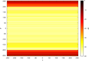
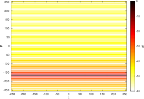
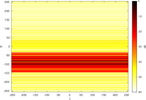
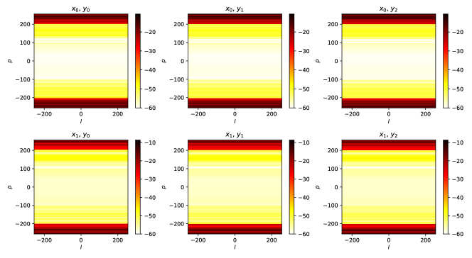
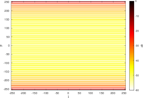
Figure 4: Discrete periodic cross-ambiguity functions for (a) a pair of Doppler-shift codes, (b) a pair of the optimized codes 𝐱𝐱\mathbf{x} and 𝐲𝐲\mathbf{y}, (c) optimized code 𝐱𝐱\mathbf{x} and an all-one code, and (d) an all-one code and optimized code 𝐲𝐲\mathbf{y}, for N=256𝑁256N=256, P=200𝑃200P=200 and Nf=512subscript𝑁𝑓512N_{f}=512.
Refer to caption
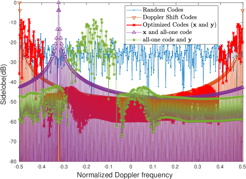
Figure 5: Comparison of the discrete periodic cross-ambiguity functions at the zero-delay cut for different scenarios for N=256𝑁256N=256, P=200𝑃200P=200 and Nf=512subscript𝑁𝑓512N_{f}=512. Although the optimized scheme achieves lower sidelobes in the desired area, the sidelobe increases in the regions outside the desired area.

In Fig. 4 and 4, the discrete PCAFs are shown for a pair of Doppler-shifting codes, and the optimized codes, respectively, where P=200𝑃200P=200 and Nf=512subscript𝑁𝑓512N_{f}=512 (which implies that the maximum Doppler frequency of interest should be lower than 3906.253906.253906.25 Hz, corresponding to a maximum relative radial velocity of 87.987.987.9 km/h). In addition, Fig. 4 and 4 show the PCAFs when one of the vehicles uses an optimized code and the other uses a non-cooperative code such as the all-one vector. It is clear from the figure that a non-cooperating interfering radar present in the scenario may ultimately fail to decrease the sidelobe in the desired region.

Fig. 5 compares the discrete periodic cross-ambiguity functions at the zero-delay cut for the above scenarios. One can observe that both Doppler shifting and optimized coding schemes achieve very low sidelobes in the desired area compared to random codes. Moreover, although the optimized scheme achieves lower sidelobes in the desired area, the sidelobe increases in the regions outside the desired area. However, for the Doppler shift coding, the sidelobes are spread evenly throughout the entire region. Therefore, they can be used to effectively suppress the interference. Further note that the peak side-lobe level (PSL) corresponding to the optimized codes is approximately 3.553.553.55 dB lower than that of the Doppler-shifting, within the desired range of Doppler frequency of interest. Interestingly, if we fix 𝐲=𝟏N𝐲subscript1𝑁\mathbf{y}=\boldsymbol{1}_{N} and only optimize 𝐱𝐱\mathbf{x}, we obtain similar results, which corresponds to a scenario where no coordination between the two radar systems is required.
Refer to caption
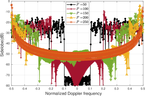
Figure 6: Comparison of the discrete PCAFs at the zero-delay cut for the optimized SISO codes with P{50,100,150,200,250}𝑃50100150200250P\in\{50,100,150,200,250\}, N=256𝑁256N=256 and Nf=512subscript𝑁𝑓512N_{f}=512.

Next, we examine the performance of the optimized SISO codes for different values of P𝑃P. In order to preserve the fairness in this experiment, we fix the maximum outer iteration number of Algorithm 1 to 100010001000 for each P𝑃P. A comparison of the sidelobe level at the zero-delay cut of the PCAFs for P{50,100,150,200,250}𝑃50100150200250P\in\{50,100,150,200,250\} is shown in Fig. 6. It can be seen from the figure that the sidelobes in the Doppler frequency of interest increase with the increase in P𝑃P. However, it is interesting to note that, once we fix ϵitalic-ϵ\epsilon in Algorithm 1 instead of fixing the maximum iteration number, the sidelobe performance in the Doppler frequency of interest improves for higher P𝑃P, however, it takes the algorithm longer to converge.
Refer to caption
Refer to caption
Refer to caption
Refer to caption
Refer to caption
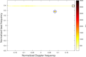
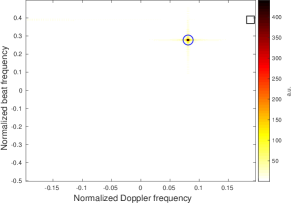
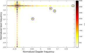
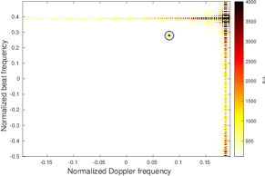
Figure 7: The range-Doppler image for (a) randomly generated code without slow-time coding, (b) Doppler-shift coding, and (c) the optimized coding scheme for the SNRs of target and interferer as 30 dB and 60 dB, respectively. Furthermore, the same for (d) Doppler-shift coding, and (e) the optimized coding scheme for the SNRs of target and interferer as 10 dB and 20 dB, respectively: \bigcirc represents the target and \Box represents the interference.

We, next, apply these coding schemes to mitigate the mutual interference for two identical automotive radar systems operating in a typical scenario: The range of target and interference are at 505050 m and 707070 m, respectively. The speeds associated with them are 10.1210.1210.12 m/s and 23.4523.4523.45 m/s. The signal-to-noise ratios (SNR) are 303030 dB and 606060 dB, respectively. The sampling frequency is fs=4subscript𝑓𝑠4f_{s}=4 MHz. M=100𝑀100M=100 samples are collected for each period. Fig. 7 (a-c) show the range-Doppler image in this scenario without slow-time coding, using Doppler-shifting code, and the optimized coding scheme, respectively. Furthermore, Fig. 7 (d-e) show the same for Doppler-shifting code and the optimized coding scheme when the SNRs are 101010 dB and 202020 dB for the target and interferer, respectively. We can observe that the power of the interference is much stronger than that of the target such that a false alarm occurs. When our slow-time coding schemes are applied, the interference power level is significantly reduced and the target can be easily detected without suffering from false alarm problems.

V-B The MIMO Scenario
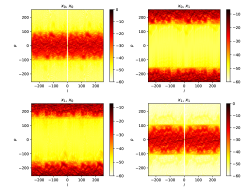
Refer to caption
Figure 8: Discrete periodic (cross) ambiguity functions between different MIMO sequences from the set 𝒳={𝐱m}m=12𝒳superscriptsubscriptsubscript𝐱𝑚𝑚12\mathcal{X}=\{\mathbf{x}_{m}\}_{m=1}^{2} for N=256𝑁256N=256, P=200𝑃200P=200 and Nf=512subscript𝑁𝑓512N_{f}=512. Note that for identical sequences, the ambiguity function always assumes larger values near zero.
Refer to caption
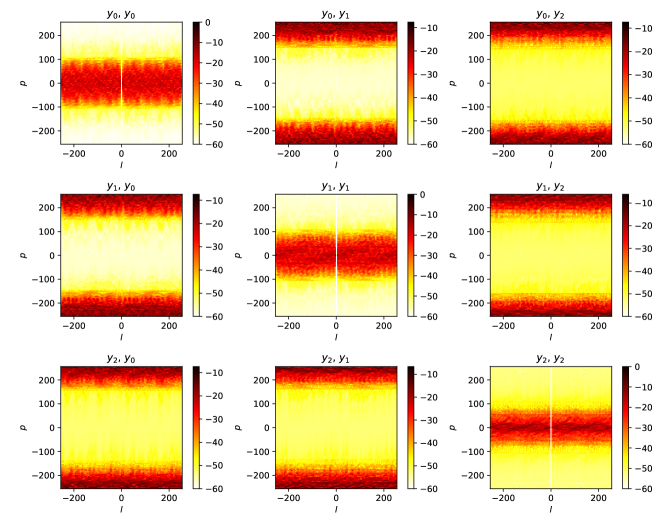
Figure 9: Discrete periodic (cross) ambiguity functions among different MIMO sequences from the set 𝒴={𝐲k}k=13𝒴superscriptsubscriptsubscript𝐲𝑘𝑘13\mathcal{Y}=\{\mathbf{y}_{k}\}_{k=1}^{3} for N=256𝑁256N=256, P=200𝑃200P=200 and Nf=512subscript𝑁𝑓512N_{f}=512.
Refer to caption
Figure 10: Discrete periodic cross-ambiguity functions between different MIMO sequences from the sets 𝒳={𝐱m}m=12𝒳superscriptsubscriptsubscript𝐱𝑚𝑚12\mathcal{X}=\{\mathbf{x}_{m}\}_{m=1}^{2} and 𝒴={𝐲k}k=13𝒴superscriptsubscriptsubscript𝐲𝑘𝑘13\mathcal{Y}=\{\mathbf{y}_{k}\}_{k=1}^{3} for N=256𝑁256N=256, P=200𝑃200P=200 and Nf=512subscript𝑁𝑓512N_{f}=512.

In order to examine the effectiveness of Algorithm 2 in the MIMO case, we use a similar set of FMCW parameters as in the SISO case. For the ease of display and sake of simplicity, we consider two similar MIMO FMCW radar systems that use set of codes 𝒳={𝐱m}m=12𝒳superscriptsubscriptsubscript𝐱𝑚𝑚12\mathcal{X}=\{\mathbf{x}_{m}\}_{m=1}^{2} and 𝒴={𝐲k}k=13𝒴superscriptsubscriptsubscript𝐲𝑘𝑘13\mathcal{Y}=\{\mathbf{y}_{k}\}_{k=1}^{3} each of length N=256𝑁256N=256, operating under the same carrier frequency of fc=24subscript𝑓𝑐24f_{c}=24 GHz, the bandwidth of the chirp signal of B=150𝐵150B=150 MHz, and the sweep time of Tc=50subscript𝑇𝑐50T_{c}=50 μ𝜇\mus. As mentioned earlier, we first initialize the algorithm with normally distributed random numbers for all optimization variables: {𝐱m}subscript𝐱𝑚\{\mathbf{x}_{m}\}, {𝐲k}subscript𝐲𝑘\{\mathbf{y}_{k}\} {𝐮l,p,mc}subscriptsuperscript𝐮𝑐𝑙𝑝𝑚\{\mathbf{u}^{c}_{l,p,m}\}, {𝐯l,p,kc}subscriptsuperscript𝐯𝑐𝑙𝑝𝑘\{\mathbf{v}^{c}_{l,p,k}\}, for c{r,i}𝑐𝑟𝑖c\in\{r,i\}. After running the algorithm once, we use the output codes {𝐱m}subscript𝐱𝑚\{\mathbf{x}_{m}\}, {𝐲k}subscript𝐲𝑘\{\mathbf{y}_{k}\} as the initial codes for the next run but we still use random initialization for other variables, {𝐮l,p,mc}subscriptsuperscript𝐮𝑐𝑙𝑝𝑚\{\mathbf{u}^{c}_{l,p,m}\}, {𝐯l,p,kc}subscriptsuperscript𝐯𝑐𝑙𝑝𝑘\{\mathbf{v}^{c}_{l,p,k}\}, and repeat the process multiple times.

Figs. 8-10 show the periodic (cross) ambiguity functions for the radar systems: {𝒳},{𝒴}𝒳𝒴\{\mathcal{X}\},\{\mathcal{Y}\}, and {𝒳,𝒴}𝒳𝒴\{\mathcal{X},\mathcal{Y}\} where P=200𝑃200P=200 and Nf=512subscript𝑁𝑓512N_{f}=512. It is evident from each of these figures that for each set of sequences, the unambiguous regions are well separated (within the range of -40dB to -60dB), and hence, these sequences can be reliably used in MIMO FMCW radar systems that require mutual interference mitigation.

In the next example for the MIMO case, we apply the optimized coding scheme to mitigate the mutual interference in the presence of multiple targets. For this scenario, we use three targets and one interfering radar system. The ranges of the targets and interference are at 50,20,6050206050,20,60 m, and 707070 m, respectively. The speeds associated with them are 10.12,5.75,7.3410.125.757.3410.12,-5.75,7.34 m/s and 23.4523.4523.45 m/s. The SNRs are 303030 dB and 606060 dB for the targets and interference, respectively. The sampling frequency is similarly fs=4subscript𝑓𝑠4f_{s}=4 MHz as assumed in the SISO case. Fig. 11 shows the range-Doppler (RD) image for different scenarios. The RD images are shown for randomly generated MIMO codes without slow-time coding, and the optimized MIMO coding scheme in Fig. 11 and  11, respectively. It is clear from the figure that the interference power level for the optimized codes is significantly reduced and all three of the targets are easily detected without suffering from false alarm issues. Furthermore, Fig. 11 shows the RD image when the interferer uses a non-cooperating all-one vector code as described in the SISO case. It is interesting to see that the presence of a strong interferer that does not respect the code usage protocol may significantly hinder the target detection capabilities.
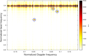
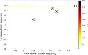
Refer to caption
Refer to caption
Refer to caption
Figure 11: The range-Doppler image for (a) randomly generated MIMO codes without slow-time coding, (b) the optimized MIMO coding scheme, and (c) optimized MIMO scheme, however the interferer uses a non-cooperating all-one vector code: \bigcirc represents the targets and \Box represents the interference.

VI Conclusion

In this paper, we discussed the problem of mutual interference mitigation in identical or similar radar systems employed in automotive applications. We proposed two slow-time coding schemes for the SISO case. Specifically, the first coding scheme is designed through Doppler shifting and the second one is devised based on an efficient cyclic optimization approach. We further extended the problem formulation and proposed another efficient algorithm to generate the radar codes in the more general MIMO scenario. We showed that these coding schemes can be used to reduce the interference power level significantly. Note that these coding schemes are highly effective when the radar parameters are nearly identical, however, the requirement of having identical parameters is not necessary.

Appendix A Efficient Computation of 𝐁xsubscript𝐁𝑥\mathbf{B}_{x} and 𝐁ysubscript𝐁𝑦\mathbf{B}_{y}

Note that 𝐁ysubscript𝐁𝑦\mathbf{B}_{y} in (22) can be rewritten as

𝐁y=p=PPDiag(𝐟p)(l=N+1N1𝐂l𝐲𝐲H𝐂lH)Diag(𝐟p)H.subscript𝐁𝑦superscriptsubscript𝑝𝑃𝑃Diagsubscript𝐟𝑝superscriptsubscript𝑙𝑁1𝑁1subscript𝐂𝑙superscript𝐲𝐲𝐻superscriptsubscript𝐂𝑙𝐻Diagsuperscriptsubscript𝐟𝑝𝐻\mathbf{B}_{y}=\sum_{p=-P}^{P}\mathrm{Diag}\left(\mathbf{f}_{p}\right)\left(\sum_{l=-N+1}^{N-1}\mathbf{C}_{l}\mathbf{y}\mathbf{y}^{H}\mathbf{C}_{l}^{H}\right)\mathrm{Diag}\left(\mathbf{f}_{p}\right)^{H}. (69)

Define 𝐑=l=N+1N1𝐂l𝐲𝐲H𝐂lH𝐑superscriptsubscript𝑙𝑁1𝑁1subscript𝐂𝑙superscript𝐲𝐲𝐻superscriptsubscript𝐂𝑙𝐻\mathbf{R}=\sum_{l=-N+1}^{N-1}\mathbf{C}_{l}\mathbf{y}\mathbf{y}^{H}\mathbf{C}_{l}^{H}. It is easy to verify 𝐑y=2𝐑0𝐲𝐲Hsubscript𝐑𝑦2subscript𝐑0superscript𝐲𝐲𝐻\mathbf{R}_{y}=2\mathbf{R}_{0}-\mathbf{y}\mathbf{y}^{H}, considering that for l<0𝑙0l<0, 𝐂l𝐲=𝐂Nl𝐲subscript𝐂𝑙𝐲subscript𝐂𝑁𝑙𝐲\mathbf{C}_{l}\mathbf{y}=\mathbf{C}_{N-l}\mathbf{y}, and 𝐑0=l=0N1𝐂l𝐲𝐲H𝐂lHsubscript𝐑0superscriptsubscript𝑙0𝑁1subscript𝐂𝑙superscript𝐲𝐲𝐻superscriptsubscript𝐂𝑙𝐻\mathbf{R}_{0}=\sum_{l=0}^{N-1}\mathbf{C}_{l}\mathbf{y}\mathbf{y}^{H}\mathbf{C}_{l}^{H}. Moreover, we can write 𝐑0subscript𝐑0\mathbf{R}_{0} as

𝐑0=𝐘𝐘H,subscript𝐑0superscript𝐘𝐘𝐻\mathbf{R}_{0}=\mathbf{Y}\mathbf{Y}^{H}, (70)

where

𝐘=[y1y2yN1yNy2y3yNy1yNy1yN2yN1].𝐘matrixsubscript𝑦1subscript𝑦2subscript𝑦𝑁1subscript𝑦𝑁subscript𝑦2subscript𝑦3subscript𝑦𝑁subscript𝑦1subscript𝑦𝑁subscript𝑦1subscript𝑦𝑁2subscript𝑦𝑁1\mathbf{Y}=\begin{bmatrix}y_{1}&y_{2}&\cdots&y_{N-1}&y_{N}\\ y_{2}&y_{3}&\cdots&y_{N}&y_{1}\\ \vdots&\vdots&\cdots&\vdots&\vdots\\ y_{N}&y_{1}&\cdots&y_{N-2}&y_{N-1}\\ \end{bmatrix}. (71)

As a result, 𝐑0subscript𝐑0\mathbf{R}_{0} can be written as

𝐑0=[cy,0cy,1cy,N2cy,N1cy,1cy,0cy,N3cy,N2cy,N1cy,N2cy,1cy,0],subscript𝐑0matrixsubscript𝑐𝑦0subscript𝑐𝑦1subscript𝑐𝑦𝑁2subscript𝑐𝑦𝑁1superscriptsubscript𝑐𝑦1subscript𝑐𝑦0subscript𝑐𝑦𝑁3subscript𝑐𝑦𝑁2superscriptsubscript𝑐𝑦𝑁1superscriptsubscript𝑐𝑦𝑁2superscriptsubscript𝑐𝑦1subscript𝑐𝑦0\mathbf{R}_{0}=\begin{bmatrix}c_{y,0}&c_{y,1}&\cdots&c_{y,N-2}&c_{y,N-1}\\ c_{y,1}^{*}&c_{y,0}&\cdots&c_{y,N-3}&c_{y,N-2}\\ \vdots&\vdots&\cdots&\vdots&\vdots\\ c_{y,N-1}^{*}&c_{y,N-2}^{*}&\cdots&c_{y,1}^{*}&c_{y,0}\\ \end{bmatrix},

where cy,l=n=1Nyny(n+l)modN,l=0,1,,N1formulae-sequencesubscript𝑐𝑦𝑙superscriptsubscript𝑛1𝑁subscript𝑦𝑛subscriptsuperscript𝑦𝑛𝑙mod𝑁𝑙01𝑁1c_{y,l}=\sum_{n=1}^{N}y_{n}y^{*}_{(n+l)\textrm{mod}N},l=0,1,\cdots,N-1. It should be noted that 𝐑0subscript𝐑0\mathbf{R}_{0} is a circulant matrix and its elements are determined by the values of the sequence {cy,l}l=0N1superscriptsubscriptsubscript𝑐𝑦𝑙𝑙0𝑁1\{c_{y,l}\}_{l=0}^{N-1}. Moreover, this sequence can be seen as the circular convolution between {yn}n=1Nsuperscriptsubscriptsubscript𝑦𝑛𝑛1𝑁\{y_{n}\}_{n=1}^{N} and {yn}n=1Nsuperscriptsubscriptsubscript𝑦𝑛𝑛1𝑁\{y_{n}\}_{n=1}^{N}, and hence can be efficiently computed via FFT operations. Therefore, the computation of 𝐑ysubscript𝐑𝑦\mathbf{R}_{y} requires 𝒪(N2)𝒪superscript𝑁2\mathcal{O}\left(N^{2}\right) flops (mainly due to the computation of 𝐲𝐲Hsuperscript𝐲𝐲𝐻\mathbf{y}\mathbf{y}^{H}).

It follows that 𝐁ysubscript𝐁𝑦\mathbf{B}_{y} can be calculated efficiently using the following result:

𝐁ysubscript𝐁𝑦\displaystyle\mathbf{B}_{y} =p=PPDiag(𝐟p)𝑹yDiag(𝐟p)Habsentsuperscriptsubscript𝑝𝑃𝑃Diagsubscript𝐟𝑝subscript𝑹𝑦Diagsuperscriptsubscript𝐟𝑝𝐻\displaystyle=\sum_{p=-P}^{P}\mathrm{Diag}\left(\mathbf{f}_{p}\right)\boldsymbol{R}_{y}\mathrm{Diag}\left(\mathbf{f}_{p}\right)^{H}
=p=PP𝐑y(𝐟p𝐟pH)absentsuperscriptsubscript𝑝𝑃𝑃direct-productsubscript𝐑𝑦subscript𝐟𝑝superscriptsubscript𝐟𝑝𝐻\displaystyle=\sum_{p=-P}^{P}\mathbf{R}_{y}\odot(\mathbf{f}_{p}\mathbf{f}_{p}^{H})
=𝐑y(𝐅P𝐅PH),absentdirect-productsubscript𝐑𝑦subscript𝐅𝑃superscriptsubscript𝐅𝑃𝐻\displaystyle=\mathbf{R}_{y}\odot(\mathbf{F}_{P}\mathbf{F}_{P}^{H}), (72)

where 𝐅P=[𝐟P,,𝐟P]N×(2P+1)subscript𝐅𝑃subscript𝐟𝑃subscript𝐟𝑃superscript𝑁2𝑃1\mathbf{F}_{P}=[\mathbf{f}_{-P},\cdots,\mathbf{f}_{P}]\in\mathbb{C}^{N\times(2P+1)}.

Finally, we consider reducing the computational complexity of computing 𝐁xsubscript𝐁𝑥\mathbf{B}_{x}. To this end, we note that

𝐁xsubscript𝐁𝑥\displaystyle\mathbf{B}_{x} =l=N+1N1𝐂lH(p=PPDiag(𝐟p)H𝐱𝐱HDiag(𝐟p))𝐂labsentsuperscriptsubscript𝑙𝑁1𝑁1superscriptsubscript𝐂𝑙𝐻superscriptsubscript𝑝𝑃𝑃Diagsuperscriptsubscript𝐟𝑝𝐻superscript𝐱𝐱𝐻Diagsubscript𝐟𝑝subscript𝐂𝑙\displaystyle=\sum_{l=-N+1}^{N-1}\mathbf{C}_{l}^{H}\left(\sum_{p=-P}^{P}\mathrm{Diag}\left(\mathbf{f}_{p}\right)^{H}\mathbf{x}\mathbf{x}^{H}\mathrm{Diag}\left(\mathbf{f}_{p}\right)\right)\mathbf{C}_{l}
=l=N+1N1𝐂lH((𝐱𝐱H)(𝐅P𝐅PT))𝐂l.absentsuperscriptsubscript𝑙𝑁1𝑁1superscriptsubscript𝐂𝑙𝐻direct-productsuperscript𝐱𝐱𝐻superscriptsubscript𝐅𝑃subscriptsuperscript𝐅𝑇𝑃subscript𝐂𝑙\displaystyle=\sum_{l=-N+1}^{N-1}\mathbf{C}_{l}^{H}\left((\mathbf{x}\mathbf{x}^{H})\odot(\mathbf{F}_{P}^{*}\mathbf{F}^{T}_{P})\right)\mathbf{C}_{l}. (73)

Let 𝐑x=(𝐱𝐱H)(𝐅P𝐅PT)subscript𝐑𝑥direct-productsuperscript𝐱𝐱𝐻superscriptsubscript𝐅𝑃subscriptsuperscript𝐅𝑇𝑃\mathbf{R}_{x}=(\mathbf{x}\mathbf{x}^{H})\odot(\mathbf{F}_{P}^{*}\mathbf{F}^{T}_{P}). We can observe that 𝐂lH𝐑x𝐂lsuperscriptsubscript𝐂𝑙𝐻subscript𝐑𝑥subscript𝐂𝑙\mathbf{C}_{l}^{H}\mathbf{R}_{x}\mathbf{C}_{l} can be computed very efficiently, since it only involves the permutation of the rows and columns of 𝐑xsubscript𝐑𝑥\mathbf{R}_{x}. Therefore, the computation of 𝐁ysubscript𝐁𝑦\mathbf{B}_{y} only requires 𝒪(N2)𝒪superscript𝑁2\mathcal{O}\left(N^{2}\right) flops.

References

  • [1] B. Tang, W. Huang, and J. Li, “Slow-time coding for mutual interference mitigation,” in 2018 IEEE International Conference on Acoustics, Speech and Signal Processing (ICASSP), 2018, pp. 6508–6512.
  • [2] S. M. Patole, M. Torlak, D. Wang, and M. Ali, “Automotive radars: A review of signal processing techniques,” IEEE Signal Processing Magazine, vol. 34, no. 2, pp. 22–35, 2017.
  • [3] Martin Schneider, “Automotive radar: Status and trends,” in In Proceedings of the German Microwave Conference GeMIC 2005, 2005, pp. 144–147.
  • [4] H. Rohling, “Milestones in radar and the success story of automotive radar systems,” in 11-th International Radar Symposium, 2010, pp. 1–6.
  • [5] J. Dickmann, J. Klappstein, M. Hahn, N. Appenrodt, H. Bloecher, K. Werber, and A. Sailer, “Automotive radar the key technology for autonomous driving: From detection and ranging to environmental understanding,” in IEEE Radar Conference (RadarConf), 2016, pp. 1–6.
  • [6] Fulvio Gini, Antonio De Maio, and Lee Patton, Waveform design and diversity for advanced radar systems, Institution of engineering and technology, London, 2012.
  • [7] Jaime Lien, Nicholas Gillian, M. Emre Karagozler, Patrick Amihood, Carsten Schwesig, Erik Olson, Hakim Raja, and Ivan Poupyrev, “Soli: Ubiquitous gesture sensing with millimeter wave radar,” ACM Trans. Graph., vol. 35, no. 4, July 2016.
  • [8] Saiwen Wang, Jie Song, Jaime Lien, Ivan Poupyrev, and Otmar Hilliges, “Interacting with soli: Exploring fine-grained dynamic gesture recognition in the radio-frequency spectrum,” in Proceedings of the 29th Annual Symposium on User Interface Software and Technology, New York, NY, USA, 2016, UIST ’16, p. 851–860, Association for Computing Machinery.
  • [9] Sergio Saponara, Maria Sabrina Greco, and Fulvio Gini, “Radar-on-chip/in-package in autonomous driving vehicles and intelligent transport systems: opportunities and challenges,” IEEE Signal Processing Magazine, vol. 36, no. 5, pp. 71–84, 2019.
  • [10] Maria S Greco, Jian Li, Teng Long, and Abdelhak Zoubir, “Advances in radar systems for modern civilian and commercial applications: Part 1 [from the guest editors],” IEEE Signal Processing Magazine, vol. 36, no. 4, pp. 13–15, 2019.
  • [11] Maria S Greco, Jian Li, Teng Long, and Abdelhak Zoubir, “Advances in radar systems for modern civilian and commercial applications: Part 2 [from the guest editors],” IEEE Signal Processing Magazine, vol. 36, no. 5, pp. 16–18, 2019.
  • [12] F. Engels, P. Heidenreich, A. M. Zoubir, F. K. Jondral, and M. Wintermantel, “Advances in automotive radar: A framework on computationally efficient high-resolution frequency estimation,” IEEE Signal Processing Magazine, vol. 34, no. 2, pp. 36–46, 2017.
  • [13] I. Bilik, O. Longman, S. Villeval, and J. Tabrikian, “The rise of radar for autonomous vehicles: Signal processing solutions and future research directions,” IEEE Signal Processing Magazine, vol. 36, no. 5, pp. 20–31, 2019.
  • [14] Shahin Khobahi, Arindam Bose, and Mojtaba Soltanalian, “Deep radar waveform design for efficient automotive radar sensing,” in 11th IEEE Sensor Array and Multichannel Signal Processing Workshop, 2020.
  • [15] S. H. Dokhanchi, B. S. Mysore, K. V. Mishra, and B. Ottersten, “A mmwave automotive joint radar-communications system,” IEEE Transactions on Aerospace and Electronic Systems, vol. 55, no. 3, pp. 1241–1260, 2019.
  • [16] S. Sedighi, B. Shankar, K. V. Mishra, and B. Ottersten, “Optimum design for sparse FDA-MIMO automotive radar,” in 2019 53rd Asilomar Conference on Signals, Systems, and Computers, 2019, pp. 913–918.
  • [17] S. H. Dokhanchi, M. R. Bhavani Shankar, K. V. Mishra, and B. Ottersten, “Multi-constraint spectral co-design for colocated MIMO radar and MIMO communications,” in Proceedings of the IEEE International Conference on Acoustics, Speech and Signal Processing (ICASSP), 2020, pp. 4567–4571.
  • [18] M. Alaee-Kerahroodi, B. Shankar, M. M. Naghsh, and B. Ottersten, “CDM-MIMO in next-generation mmWave automotive radar sensors,” in Proceedings of URSI AP-RASC, 2019.
  • [19] F. Uysal, “Synchronous and asynchronous radar interference mitigation,” IEEE Access, vol. 7, pp. 5846–5852, 2019.
  • [20] Sruthy Skaria, Akram Al-Hourani, Robin J Evans, Kandeepan Sithamparanathan, and Udaya Parampalli, “Interference mitigation in automotive radars using pseudo-random cyclic orthogonal sequences,” Sensors (Basel, Switzerland), vol. 19, no. 20, pp. 4459, Oct 2019.
  • [21] Wen-Qin Wang and Huaizong Shao, “Radar-to-radar interference suppression for distributed radar sensor networks,” Remote Sensing, vol. 6, no. 1, pp. 740–755, 2014.
  • [22] M. Goppelt, H. L. Blöcher, and W. Menzel, “Automotive radar - investigation of mutual interference mechanisms,” Advances in Radio Science, vol. 8, pp. 55–60, Sept. 2010.
  • [23] M. Goppelt, H. L. Blöcher, and W. Menzel, “Analytical investigation of mutual interference between automotive FMCW radar sensors,” in 2011 German Microwave Conference, 2011, pp. 1–4.
  • [24] A. Bourdoux, K. Parashar, and M. Bauduin, “Phenomenology of mutual interference of FMCW and PMCW automotive radars,” in 2017 IEEE Radar Conference (RadarConf), 2017, pp. 1709–1714.
  • [25] M. A. Hossain, I. Elshafiey, and A. Al-Sanie, “Mutual interference mitigation in automotive radars under realistic road environments,” in 2017 8th International Conference on Information Technology (ICIT), 2017, pp. 895–900.
  • [26] Canan Aydogdu, Musa Furkan Keskin, Gisela K. Carvajal, Olof Eriksson, Hans Hellsten, Hans Herbertsson, Emil Nilsson, Mats Rydstrom, Karl Vanas, and Henk Wymeersch, “Radar interference mitigation for automated driving: Exploring proactive strategies,” IEEE Signal Processing Magazine, vol. 37, no. 4, pp. 72–84, 2020.
  • [27] G. M. Brooker, “Mutual interference of millimeter-wave radar systems,” IEEE Transactions on Electromagnetic Compatibility, vol. 49, no. 1, pp. 170–181, 2007.
  • [28] S. Rao and A. V. Mani, “Interference characterization in FMCW radars,” in 2020 IEEE Radar Conference (RadarConf20), 2020, pp. 1–6.
  • [29] P. Wang, D. Millar, K. Parsons, and P. V. Orlik, “Nonlinearity correction for range estimation in FMCW millimeter-wave automotive radar,” in IEEE MTT-S International Wireless Symposium (IWS), 2018, pp. 1–3.
  • [30] P. Wang, P. Boufounos, H. Mansour, and P. V. Orlik, “Slow-time MIMO-FMCW automotive radar detection with imperfect waveform separation,” in IEEE International Conference on Acoustics, Speech and Signal Processing (ICASSP), 2020, pp. 8634–8638.
  • [31] M. Soltanalian and P. Stoica, “Design of perfect phase-quantized sequences with low peak-to-average-power ratio,” in Proceedings of the 20th European Signal Processing Conference (EUSIPCO), 2012, pp. 2576–2580.
  • [32] B. Friedlander, “Waveform design for MIMO radars,” IEEE Transactions on Aerospace and Electronic Systems, vol. 43, no. 3, pp. 1227–1238, 2007.
  • [33] B. Tang, J. Tuck, and P. Stoica, “Polyphase waveform design for MIMO radar space time adaptive processing,” IEEE Transactions on Signal Processing, vol. 68, pp. 2143–2154, 2020.
  • [34] J. Li, P. Stoica, L. Xu, and W. Roberts, “On parameter identifiability of MIMO radar,” IEEE Signal Processing Letters, vol. 14, no. 12, pp. 968–971, 2007.
  • [35] R. Lin, M. Soltanalian, B. Tang, and J. Li, “Efficient design of binary sequences with low autocorrelation sidelobes,” IEEE Transactions on Signal Processing, vol. 67, no. 24, pp. 6397–6410, 2019.
  • [36] A. Bose and M. Soltanalian, “Constructing binary sequences with good correlation properties: An efficient analytical-computational interplay,” IEEE Transactions on Signal Processing, vol. 66, no. 11, pp. 2998–3007, 2018.
  • [37] Augusto Aubry, Antonio De Maio, Bo Jiang, and Shuzhong Zhang, “Ambiguity function shaping for cognitive radar via complex quartic optimization,” IEEE Transactions on Signal Processing, vol. 61, no. 22, pp. 5603–5619, 2013.
  • [38] Chun-Yang Chen and PP Vaidyanathan, “MIMO radar ambiguity properties and optimization using frequency-hopping waveforms,” IEEE Transactions on Signal Processing, vol. 56, no. 12, pp. 5926–5936, 2008.
  • [39] Hao He, Petre Stoica, and Jian Li, “On synthesizing cross ambiguity functions,” in IEEE International Conference on Acoustics, Speech and Signal Processing (ICASSP). IEEE, 2011, pp. 3536–3539.
  • [40] Meisam Razaviyayn, Mingyi Hong, and Zhi-Quan Luo, “A unified convergence analysis of block successive minimization methods for nonsmooth optimization,” SIAM Journal on Optimization, vol. 23, no. 2, pp. 1126–1153, 2013.
  • [41] A. Aubry, A. De Maio, A. Zappone, M. Razaviyayn, and Z. Luo, “A new sequential optimization procedure and its applications to resource allocation for wireless systems,” IEEE Transactions on Signal Processing, vol. 66, no. 24, pp. 6518–6533, 2018.
  • [42] M. Soltanalian, B. Tang, Jian Li, and P. Stoica, “Joint design of the receive filter and transmit sequence for active sensing,” IEEE Signal Processing Letters, vol. 20, no. 5, pp. 423–426, 2013.
  • [43] M. Soltanalian and P. Stoica, “Designing unimodular codes via quadratic optimization,” IEEE Transactions on Signal Processing, vol. 62, no. 5, pp. 1221–1234, 2014.
  • [44] Bo Tang, M. M. Naghsh, and Jun Tang, “Relative entropy-based waveform design for MIMO radar detection in the presence of clutter and interference,” IEEE Transactions on Signal Processing, vol. 63, no. 14, pp. 3783–3796, 2015.
  • [45] Bo Tang and Jun Tang, “Joint design of transmit waveforms and receive filters for MIMO radar space-time adaptive processing,” IEEE Transactions on Signal Processing, vol. 64, no. 18, pp. 4707–4722, 2016.
  • [46] Mohammad Mahdi Naghsh, Mahmoud Modarres-Hashemi, Shahram ShahbazPanahi, Mojtaba Soltanalian, and Petre Stoica, “Unified optimization framework for multi-static radar code design using information-theoretic criteria,” IEEE Transactions on Signal Processing, vol. 61, no. 21, pp. 5401–5416, 2013.
  • [47] H. Hu, M. Soltanalian, P. Stoica, and X. Zhu, “Locating the few: Sparsity-aware waveform design for active radar,” IEEE Transactions on Signal Processing, vol. 65, no. 3, pp. 651–662, 2017.
  • [48] H. He, P. Stoica, and J. Li, “Designing unimodular sequence sets with good correlations—including an application to MIMO radar,” IEEE Transactions on Signal Processing, vol. 57, no. 11, pp. 4391–4405, 2009.
  • [49] J. A. Tropp, I. S. Dhillon, R. W. Heath, and T. Strohmer, “Designing structured tight frames via an alternating projection method,” IEEE Transactions on Information Theory, vol. 51, no. 1, pp. 188–209, 2005.
  • [50] J. Li, P. Stoica, and X. Zheng, “Signal synthesis and receiver design for MIMO radar imaging,” IEEE Transactions on Signal Processing, vol. 56, no. 8, pp. 3959–3968, 2008.
  • [51] Mojtaba Soltanalian, Heng Hu, and Petre Stoica, “Single-stage transmit beamforming design for MIMO radar,” Signal Processing, vol. 102, pp. 132 – 138, 2014.