Generalization and Overfitting in Matrix Product State Machine Learning Architectures

Abstract

While overfitting and, more generally, double descent are ubiquitous in machine learning, increasing the number of parameters of the most widely used tensor network, the matrix product state (MPS), has generally lead to monotonic improvement of test performance in previous studies. To better understand the generalization properties of architectures parameterized by MPS, we construct artificial data which can be exactly modeled by an MPS and train the models with different number of parameters. We observe model overfitting for one-dimensional data, but also find that for more complex data overfitting is less significant, while with MNIST image data we do not find any signatures of overfitting. We speculate that generalization properties of MPS depend on the properties of data: with one-dimensional data (for which the MPS ansatz is the most suitable) MPS is prone to overfitting, while with more complex data which cannot be fit by MPS exactly, overfitting may be much less significant.

I Introduction

One of the central tasks of machine learning is to generalize model performance to unseen data. Classical statistical theory suggests that increasing the complexity of a model reduces its bias and increases its variance Hastie et al. (2009) leading to the well known non-monotonic U-shaped behavior of test loss — see the orange dashed line in Fig. 1. This means that one observes either underfitting (high bias, low variance) at smaller model complexity or overfitting (high variance, low bias) at higher complexity. But modern practice suggests the reality is more complex. When training a model long enough without any regularization, one finds a ubiquitous double descent behavior of test loss Nakkiran et al. (2019): a U-shaped loss profile is followed by a monotonic decrease of the loss as model complexity grows — see dash–dotted green line in Fig. 1. This behavior was observed in many different architectures and different domains which suggests that more complex models generalize better.

A common and powerful model used in physics to approximate probability distributions of complex systems in exponentially high dimensional spaces is a matrix product state (MPS) Schollwöck (2011), also known as a tensor train Oseledets (2011). The expressivity of an MPS is controlled by its bond dimension, or dimension of the internal indices summed over within the network of tensors. At higher bond dimension, an MPS is able to capture longer-ranged and more complex correlations, thus resolving more details of an underlying probability distribution.

Following its success in physics applications, the MPS format has been investigated as a model architecture for machine learning tasks such as supervised learning Novikov et al. (2016); Stoudenmire and Schwab (2016); Glasser et al. (2018); Dborin et al. (2021); Wright et al. (2022); Dilip et al. (2022) and generative modeling Han et al. (2018); Cheng et al. (2019a); Bradley et al. (2020); Liu et al. (2021a); Hur et al. (2022); Nunez-Fernandez et al. (2022); Lin et al. (2021); Alcazar et al. (2021). In machine learning applications MPS and other tensor network architectures typically show improved performance as their capacity grows, determined by their bond dimension Stoudenmire and Schwab (2016). But overfitting has also been observed Martyn et al. (2020); Cheng et al. (2021). This raises a question: how does increasing MPS bond dimension affect its generalization properties, that is, its performance on unseen test data when using finite training data?

To address this question in a controlled way, we focus on a regression task using a complex artificial data set which nevertheless can be fit exactly by an MPS. By employing two different methods to obtain trained models — either inversion and compression or gradient–based optimization — we observe that a finite MPS bond dimension acts to regularize the model. When the number of training samples is not sufficient to fully specify all tensor elements and when the data is not too complex (can be well represented by a low order polynomial), there exists an optimal bond dimension $\chi^{*}$ which results in the best test performance and which is smaller than the bond dimension required to fit the data exactly. We also see that the optimal bond dimension $\chi^{*}$ generally increases as as the complexity of underlying data distribution grows or as the number of training samples goes up (increasing the amount of signal in the training set).

Figure 1: Possible scenarios of test loss dependence on a model capacity. Orange dashed line: “classical” statistics where improving test performance is followed by overfitting (U-shaped behavior). Green dash–dotted line: training with regularization, which generally leads to improved test performance as model capacity grows. Blue solid line: double descent test loss profile (no explicit regularization) generally found in most of machine learning models — see Ref. Nakkiran et al. (2019) and references therein.

The rest of the paper is organized as follows. Section II describes the techniques used: the MPS regression approach, data construction procedure, and MPS optimization methods. In Section III we present our studies based on artificial data for which we observe an overfitting phenomenon. In Section IV we present classification results using the MNIST data set LeCun et al. (2010). Section V discusses interpretation and implications of our findings and also future directions. Appendices provide further technical details.

II Data generation and regression

II.1 Regression setup

The main idea behind using tensor networks for machine learning is to map features into an exponentially high dimensional space and then perform linear regression in that space, but with compressed weights. The weights are represented by a tensor with a number of indices in correspondence to the number of inputs. This idea was introduced first in Ref. Stoudenmire and Schwab (2016); Novikov et al. (2016). While the amount of memory required to store an arbitrary tensor scales exponentially with the number of its indices, compressed tensor representations, called tensor networks, provide a trade-off between expressivity versus memory and computational costs required to compute or optimize the tensor. Usually, tensor compression improves space and time complexity from exponential to linear in the number of features.

Different tensor networks may be more suitable for particular types of data than others. For example, MPS are routinely used to model one-dimensional (1D) systems with short-range correlations, while PEPS Cheng et al. (2021) tensor networks are specifically designed for two-dimensional (2D) systems, and other architectures like tree tensor networks Stoudenmire (2018); Cheng et al. (2019b); Wall and DAguanno (2021) or MERA Reyes and Stoudenmire (2021) are useful for 1D systems with long-range correlations. In this paper we will focus on MPS as the simplest example of a tensor network.

To set up MPS based regression, we first map each scalar feature $x_{i}$ into a vector using a feature map $\phi(x_{i})$. Some common choices of a feature map are trigonometric $\phi(x_{i})=(\,\sin(x),\cos(x)\,)$ or polynomial $\phi(x_{i})=(1,x,x^{2},\ldots)$. In this paper we will use a polynomial feature map with a dimension $f=3$, namely $\phi(x_{i})=(1,x,x^{2})$. We then map the vector ${\bf x}$ of $N$ features into an $f^{N}$ dimensional space by (formally) taking the tensor product:

$${\bf x}\to\Phi^{s_{1}...s_{N}}({\bf x}) =\phi^{s_{1}}(x_{1})\phi^{s_{2}}(x_{2})\cdots\phi^{s_{N}}(x_{N})$$ (1)

where each index $s_{j}$ takes the values $1,2,\ldots,f$. Next we define a weight tensor $W$ which we parameterize as a matrix product state (MPS):

$$W^{s_{1}...s_{N}}=\sum_{i_{1},i_{2},\ldots,i_{N-1}}A^{s_{1}}_{i_{1}}A^{s_{2}}_{i_{1}i_{2}}...A^{s_{N-1}}_{i_{N-2}i_{N-1}}A^{s_{N}}_{i_{N-1}},$$ (2)

where the dimension of the “virtual”, internal, or bond indices $i_{j}$ is called the bond dimension of bond $j$. The maximum over all bond dimensions is referred to as the bond dimension $\chi$ of the MPS as a whole.

The model $f({\bf x})$ we will use for regression or classification is given by contracting the weight tensor $W$ with the feature tensor $\Phi({\bf x})$ to return a scalar:

$$f({\bf x})=W\cdot\Phi({\bf x})=\sum_{s_{1},s_{2},\ldots,s_{N}}W^{s_{1}...s_{N}}\Phi^{s_{1}...s_{N}}({\bf x})$$ (3)

To compute $f({\bf x})$ efficiently, the local feature maps are contracted one by one with the MPS tensors $A^{s_{n}}_{i_{n-1}i_{n}}$ and similar efficient contractions can be performed to obtain the gradient of each MPS tensor.

A common way to perform a learning task with a model architecture such as (3) is to define a suitable objective or “loss” function and optimize the weights such that the loss is minimized. In our calculations we will minimize mean squared error

$$\mathcal{L}=\frac{1}{2T}\sum_{i=1}^{T}\big{(}f({\bf x}^{i})-y^{i}\big{)}^{2}+\frac{\lambda}{2}|W|^{2},$$ (4)

where the summation is over $T$ training samples, $y^{i}$ is a label corresponding to the $i$-th feature vector ${\bf x}^{i}$ and the last term is a standard $L_{2}$ regularization term.

II.2 Data generation

To generate complex data whose labels can be exactly predicted by an MPS, we formulate a “target” MPS $W_{T}$ from which we generate labels for our data samples. This target MPS is distinct from the MPS that we use to parameterize our model Eq. (3).

The steps to generate our training data are:

1. Sample $N_{T}$ different feature vectors ${\bf x}^{i}$ from a multivariate Gaussian distribution

2. Apply the map $\Phi({\bf x}^{i})$

3. Compute $y^{i}=W_{T}\cdot\Phi({\bf x}^{i})$

The output of this process is a training set $\{y^{i},{\bf x}^{i}\}_{i=1}^{N_{T}}$ of size $N_{T}$.

Our choice of local feature map will be $\phi^{s_{j}}(x_{j})=(1,x_{j},x^{2}_{j})$. This makes the result of contracting a given feature tensor with an MPS also a polynomial $\sum\alpha_{p_{1}\ldots p_{N}}(x_{1})^{p_{1}}(x_{2})^{p_{2}}\ldots(x_{N})^{p_{N}}$ for some coefficients $\alpha_{p_{1}\ldots p_{N}}$. By tuning the parameters of $W_{T}$ we can always get the desired coefficients $\alpha_{p_{1}p_{2}\ldots p_{N}}$. In our experiments we set up an MPS which generates a polynomial whose degree is controlled by the MPS bond dimension. We can also control the complexity of the learning task by reducing or increasing the effect of higher order terms by varying a single control parameter $\varepsilon$, which is discussed below.

We want to construct an MPS returning an n-th order polynomial with reduced effect of higher order terms. This can be ensured by a particular choice of matrices constituting MPS tensors. Let us consider the following structure for the MPS parameterization of $W_{T}$:

$$\begin{pmatrix}...\\ ...\\ \vdots\end{pmatrix}\begin{pmatrix}I\\ M\ x_{2}\\ M^{2}\ x_{2}^{2}\\ \vdots\\ M^{f-1}x_{2}^{f-1}\end{pmatrix}\dots\begin{pmatrix}I\\ M\ x_{n-1}\\ M^{2}\ x_{n-1}^{2}\\ \vdots\\ M^{f-1}\ x_{n-1}^{f-1}\end{pmatrix}\begin{pmatrix}\vdots&\vdots&\dots\end{pmatrix},$$ (5)

where $f$ is the feature map dimension, the first matrix dimension is $f\times\chi$ ($\chi$ is the bond dimension), and the last matrix dimension is $\chi\times f$, $I$ is an identity matrix. Here $M$ is a matrix which we will determine below and $M^{k}$ means $M$ to the power of $k$. In the expression (5) above, we are viewing each MPS tensor $A^{s_{j}}_{i_{j-1}i_{j}}$ as a vector of matrices, which is an equivalent way of thinking of a tensor with three indices: the vector index is the feature index $s_{j}$ and the matrix indices are the left and right virtual or bond indices of the MPS.

To obtain an $n$-th order polynomial as our target function, we may choose nilpotent matrices with index $n+1$, meaning $M^{n+1}=0$. For example, any $L$-dimensional triangular matrix with zeros along the main diagonal is nilpotent, with index $n\leq L$. This implies that with this choice of $M$-matrices, to get an $n$-th order polynomial, the bond dimension must be at least $n+1$. For example, to generate the second order polynomial, one may choose the following order $3$ nilpotent $M$ matrix:

$$M=\begin{pmatrix}0&\varepsilon&0\\ 0&0&\varepsilon\\ 0&0&0\end{pmatrix},M^{2}=\begin{pmatrix}0&0&\varepsilon^{2}\\ 0&0&0\\ 0&0&0\end{pmatrix},M^{3}=\begin{pmatrix}0&0&0\\ 0&0&0\\ 0&0&0\end{pmatrix},$$ (6)

where the value of $\varepsilon<1$ controls the effect of higher order terms, which means that each $n$-th order term has a prefactor $\varepsilon^{n}$. In general, we can consider more general nilpotent matrices $UMU^{\dagger}$, where $U$ is a random unitary matrix.

We noticed that the data generated this way is challenging to fit: the distribution of labels $y^{i}$ is very broad and gets even broader as one includes higher order terms or increases their effect. Therefore, to be able to fit the data efficiently, we normalize labels by subtracting their mean and dividing by the standard deviation $y^{i}\to(y^{i}-\text{mean}(y))/\text{std}(y)$. Note that despite this post-processing step, one can show that the training data can still be fit perfectly by a model whose weight MPS $W$ has the same bond dimension as the MPS defining $W_{T}$.

II.3 Optimization

There are multiple strategies to optimize an MPS for a supervised learning task. One method is the density matrix renormalization group (DMRG) algorithm which is the gold standard in physics applications and involves optimizing one or two MPS tensors at a time, sweeping back and forth over the MPS Schollwöck (2011). Another option is gradient descent in the style of back-propagation, updating every MPS tensor in parallel at each optimization step Hauru et al. (2021). And there are other alternatives such as Riemannian optimization Novikov et al. (2016).

We found the DMRG approach to be convenient and efficient, optimizing one MPS tensor at a time using conjugate gradient descent based on the ITensor software Fishman et al. (2020) and the OptimKit.jl library (see details in Appendix B).

One issue we had with DMRG, however, was a strong dependence of final results on initial conditions. To avoid this issue we developed a second approach based on exact inversion and compression. Although the cost of solving for and storing the entire weight tensor $W$ becomes prohibitively large with an increasing number of features, and corresponding number of tensor indices, one can still obtain the weight tensor exactly for relatively small problems. To find the exact solution, we set the derivative of the loss, Eq. (4), to zero which results in linear algebra problem one can solve numerically exactly for $W$. After finding the exact weight tensor this way, we compress it into an MPS of some desired bond dimension through a sequence of singular value decompositions. When using this inversion and compression method we limited our problem size to only have six features. For more details about this method, see Appendix 9.

While the results obtained via inversion and compression are consistent, meaning they do not depend on any initialization, they may be suboptimal as the tensor compression step does not guarantee that the resulting MPS is necessarily optimal in the sense of perfectly minimizing the loss. Therefore, below we will also present the results of DMRG optimization initialized by the inversion and compression method.

Regardless of the optimization method chosen, the results still depend on the particular training data set used. Therefore we generate multiple training data sets and a single test set from the same probability distribution, run independent calculations for each training set, and average the results to obtain the dependence of loss function on the MPS bond dimension with corresponding error bars.

The source code used for all the experiments in this article can be accessed at git .

III Results with artificial data

In our calculations we use data ${\bf x}$ of dimension $N=6$ and feature map dimension $f=3$, i.e. each scalar feature is mapped into a vector $\phi(x)=(1,x,x^{2})$. The target MPS $W_{T}$ has the maximum possible bond dimension which for $N=6$ and $f=3$ gives a bond dimension of $\chi=27$ at the center bond. Below we present the results of inversion and compression and support them with optimization results, which are much more computationally expensive but which can outperform the inversion ones.

In Figures 2 and 3 we show the results obtained when using the inversion and compression method to train the model. Figure 2 shows the test loss versus bond dimension as the number of training samples increases.

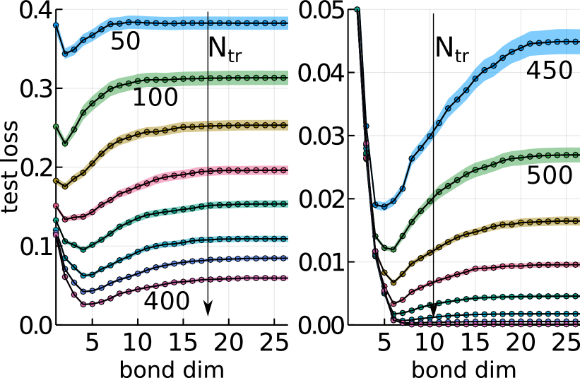
Figure 2: Test loss resulting from MPS optimized with the inversion and compression (bond dimension reduction) method. The test set used has $N_{\text{test}}=1024$ samples. The curves show the mean value of test loss and shaded regions show one standard deviation $\pm\sigma$ when averaging results over $100$ training data sets. The $L_{2}$ regularization used was $10^{-6}$ and MPS complexity parameter used was $\varepsilon=0.3$. Different curves correspond to changing the number of $N_{\text{tr}}$ samples in each training set used from $50$ to $800$ in steps of $50$ (top to bottom).

When the number of training samples is not sufficient to fully fix the weight tensor (which is generally the case), we can clearly see a minimum at a bond dimension $\chi^{*}$, which is much smaller than maximum bond dimension. We call $\chi^{*}$ the optimal bond dimension since it yields the best generalization. The optimal bond dimension goes up as we increase the number of training samples. This makes sense as the training set becomes more representative of the true data distribution (contains more signal) and the larger MPS bond dimension allows a better fit to this data, correspondingly resolving finer details of an underlying distribution. We also get nearly perfect performance when the number of training samples $N_{\text{tr}}\geq f^{N}$ is sufficient to fully characterise the weight tensor, which happens when the number of samples reaches $f^{N}$ ($=3^{6}=729$ in our case).

Figure 3 shows the evolution of the test loss dependence of an MPS bond dimension as the effect of higher order terms varies by means of changing data generating MPS control parameter $\varepsilon$.

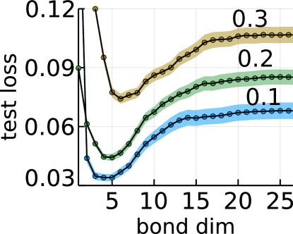
Figure 3: Test loss as a function of MPS bond dimension for increasing values of the data complexity parameter $\varepsilon$ from $0.1$ to $0.3$. The inversion and compression method was used to train the model with an $L_{2}$ regularization of $10^{-6}$. Curves show the mean value and shaded regions one standard deviation when averaged over $100$ data sets. Each training set consisted of $N_{\text{tr}}=300$ samples and the test set had $N_{\text{test}}=1024$ samples.

As $\varepsilon$ increases, the effect of higher order terms becomes more pronounced and the data essentially becomes more complex. This leads to the optimal bond dimension $\chi^{*}$ being shifted towards higher values required to resolve more delicate details of data.

While the procedure described above is numerically cheap and efficient, it does not guarantee that the results are optimal for all bond dimensions, only for the largest bond dimension. This is because the tensor compression step of our inversion and compression procedure only guarantees that the MPS we obtain is the closest MPS to the original, optimal tensor in $L_{2}$ norm, which is of course different from minimizing the loss directly. To verify the robustness of our conclusions, we now turn to DMRG optimization, which directly minimizes the loss at a fixed bond dimension but is more numerically costly in our case.

To verify that we obtain similar results when using DMRG optimization to train our model, we focus on a particular training set size $N_{\text{tr}}=300$ and target model complexity $\varepsilon=0.1,0.3$ (which is small enough reflecting our assumption that the data can be efficiently modeled by a low order polynomial of features thus making an MPS a good enough weight ansatz for such purposes). We sample several training sets and and run both inversion and compression as well as DMRG optimization on each of them. Results for other training data set sizes and complexities $\varepsilon$ are shown in Appendix D and qualitatively agree with the results presented in this section.

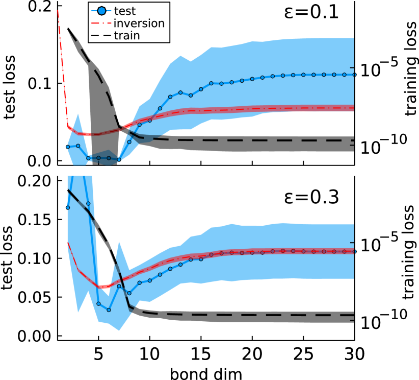
Figure 4: The results of DMRG optimization at various MPS bond dimensions averaged over 32 training data sets each of size $N_{\text{tr}}=300$. The complexity parameter of the target distribution was $\varepsilon=0.1,0.3$ (top and bottom panels respectively). The test set size used was $N_{\text{test}}=1024$. The dash–dotted red line and the corresponding shaded region show the mean test loss obtained using the inversion and compression method with one sigma standard deviation. The blue line (with shaded regions corresponding to one sigma standard deviation) shows the mean value of test loss at the model state corresponding to the best validation loss. The black dashed line shows mean training loss (and shaded region showing one standard deviation).

In Fig. 4 we show the resulting loss values obtained with both optimization methods. We can see that overall the inversion and compression approach returns very good results despite not involving the loss function in the compression step of the procedure. Only in the vicinity of optimal bond dimension does additional DMRG optimization consistently improve model performance. As in the other results above, we can clearly see that the test loss starts degrading (increasing) beyond a certain bond dimension while the training loss continues to improve. Overall, our DMRG optimization results confirm what we observed with the inversion and compression method: that overfitting occurs beyond a certain bond dimension $\chi^{*}$ whose value depends on the size of the training set and complexity of the underlying data distribution.

IV Results with MNIST

The results obtained with artificial data show that the best performance on unseen test data happens for a finite MPS bond dimension, suggesting that limiting the bond dimension may be a good strategy to improve generalization and prevent overfitting. In this section we check whether this conclusion holds for the task of supervised learning of the MNIST data set of handwritten digits. For these experiments we will be using cross-entropy loss function, discussed in Appendix C.

When using the full training set of MNIST images, we see that training accuracy steadily improves as the bond dimension grows, although in our experiments the training accuracy never reached hundred per cent for the full MNIST training set (not shown). Inspired by Ref. Nakkiran et al. (2019), which shows that the second descent of training loss occurs when perfect training accuracy is reached, we reduce the number of training images to $1024$ so that we can attain this limit.

In the top panel of Fig. 5 we plot training and test set accuracies versus MPS bond dimension at a fixed training set size $N_{\text{tr}}=1024$ and test set size $N_{\text{test}}=10,000$. The model reaches perfect training accuracy at bond dimension $\chi=6$ and we do not see any test accuracy drop or recovery in the vicinity of $\chi=6$. Overall, the test set accuracy only continues to improve as the bond dimension is increased and we do not see any indication of double descent behavior (even when introducing label noise as proposed in Ref. Nakkiran et al. (2019) — see Fig. 9 in Appendix E). Moreover, we also do not see any overfitting of the kind we observed in our artificial data experiments. In other words, we essentially see a single descent. We note that it could be possible that as we increased the bond dimension $\chi$, we simply overshot a small range of bond dimensions where the test set accuracy would show a double-descent feature. One reason this could be possible is that the number of parameters in our model grows quadratically with $\chi$, so rather quickly.

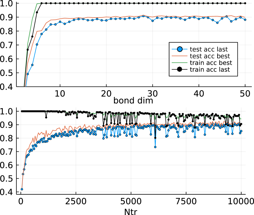
Figure 5: The results of optimization obtained with a sweeping algorithm at fixed bond dimension for an MNIST data set. Top panel shows the best test loss and training and test losses at the last training step (100 full DMRG sweeps — from left to right and right to left — with 5 conjugate gradient steps per MPS tensor) using $1024$ training images. Bottom panel shows losses versus the number of training images using an MPS of fixed bond dimension $\chi=6$.

To further investigate whether overfitting or double descent might be possible, we follow a procedure similar to one in Ref. Nakkiran (2019) by fixing MPS bond dimension $\chi=6$ and varying the number of training samples. In the lower panel of Fig. 5 we plot corresponding accuracies. Although the results are a bit noisy, overall they show monotonic improvement of test set accuracy (and degrading training accuracy) as the number of training samples increases. This is in contrast with the results of Ref. Nakkiran (2019), which show strongly degraded test performance in the vicinity of $N_{\text{tr}}$, which corresponds to transition between perfect and imperfect fitting of training data, which would happen around $N_{\text{tr}}\approx 1000$ in our case.

Therefore, surprisingly with the MNIST data as we increase the MPS bond dimension we neither see overfitting, which we see with our artificial data, nor do we see double descent which has been observed in many other machine learning architectures. One possibility is that overfitting or a double descent simply occurs at much larger bond dimensions than we reached. But this is unlikely as in the top panel of Fig. 5 we pushed the bond dimension far beyond one required for perfect interpolation, that is, achieving zero training error. Another explanation could come from the essentially different nature of the artificial and MNIST data sets. The artificial data is in some sense one-dimensional as it is created by an MPS and can be exactly fitted by an MPS, while MNIST data is two-dimensional, for which MPS is not ideally suited in principle. Indeed, as was shown in Ref. Cheng et al., 2021, two-dimensional PEPS tensor network architectures do show overfitting with MNIST and quasi-two-dimensional block-MPS architectures in Ref. Martyn et al., 2020 show overfitting as well. Therefore, we speculate that the fitting and generalization properties of tensor networks not only differ from other machine learning architectures, but also depend on the data itself.

To illustrate the last point, we construct an artificial dataset with $\varepsilon=1.0$, therefore making the data too complex to be efficiently fit by an MPS of a fixed (not exponentially large) bond dimension. In Fig. 6 we show the results of inversion with compression and DMRG optimization. We can see that with more complex data overfitting is much weaker and so increasing the bond dimension does not lead to pronounced U-shape behaviour of test loss as in Fig. 4 for less complex data. This further suggest that generalization properties of tensor networks can depend on the combination of their architecture and the properties of the data.

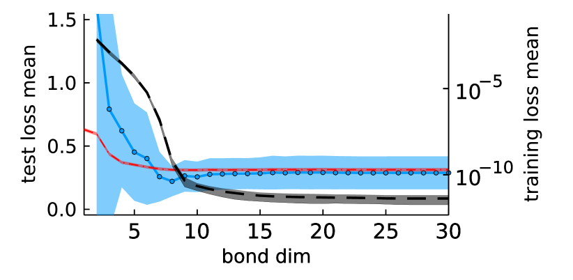
Figure 6: The results of DMRG optimization at various MPS bond dimensions averaged over 32 training data sets each of size $N_{\text{tr}}=300$. The complexity parameter of the target distribution was $\varepsilon=1.0$. All other parameters and lines are as in Fig. 4.

V Discussion

We studied the generalization properties of MPS based models using artificial data and as well as more realistic MNIST image data. Our results with artificial data show overfitting for large enough MPS bond dimensions $\chi$, such that limiting $\chi$ to a finite value typically improves model performance on unseen test data. In contrast, we found for MNIST that increasing $\chi$ always improved test performance, leading to a “single descent” and no overfitting.

We did not find any signatures of the double descent behavior frequently observed in other model architectures, such as in Refs. Nakkiran et al., 2019; Nakkiran, 2019. Of course there is no guarantee that the MPS regression approach should exhibit double descent, as it is different in many respects from other established machine learning techniques. But the presence or absence of the double descent phenomenon should be investigated further for MPS using other data sets and larger bond dimensions. The same line of investigation should also be pursued for more expressive types of tensor networks such as tree tensor networks Stoudenmire (2018); Cheng et al. (2019b), block MPS Martyn et al. (2020), or PEPS Cheng et al. (2021) The generalization and overfitting behavior of other features maps used in conjunction with MPS should also be investigated, such as feature maps based on data “amplitude encoded” as MPS Wright et al. (2022); Dilip et al. (2022).

One lesson highlighted by our observation of overfitting is the very different settings of training an MPS on a finite amount of data versus optimizing an MPS for a fully specified problem. Historically, the most common application of MPS has been for solving partial differential equations, most notably the Schrödinger equation in quantum physics. For such problems, increasing the bond dimension can always yield more accurate results because the differential operator is exactly specified. But when using MPS to model sampled data, our results show that continuing to increase the bond dimension may not always lead to better outcomes due to the statistical variance inherent to a training set of a finite size.

Another issue we encountered in our work is that training tensor network models can be difficult in certain cases. For example, in Ref. Liu et al. (2021b) it was shown that barren plateaus (regions of an exponentially vanishing gradient and thus inefficient training) are very common with MPS when using a global loss function. On the other hand, MPS training on the MNIST is very efficient, while on the artificial data (which can be fit exactly by an MPS) training turned out to be much more challenging, which suggests that trainability depends not only on the type of model, but on the data itself.

Finally, our differing results for the artificial data versus MNIST image data highlights the need to study what kind of data can be efficiently modeled by different kinds of tensor networks. Work along these lines is already under way Convy et al. (2022); Lu et al. (2021); Martyn et al. (2020) but open questions remain. For example, while exact calculations show that MPS cannot efficiently capture certain distributions of two-dimensional image data Martyn et al. (2020), approximating these same distributions with finite bond dimension MPS nevertheless yields good unsupervised and supervised model performance Lin et al. (2021); Wright et al. (2022). Understanding how MPS and other tensor networks capture data sets will not only lead to better practices for machine learning, but could also spur progress toward more ambitious goals such as a classification of data.

Supplementary Material for “MPS generalization: bond dimension effect”

Appendix A Inversion and compression

We want to minimize the loss function

$$\mathcal{L}=\frac{1}{2T}\sum_{i=1}^{T}\left(\Phi_{\xi}({\bf x}^{i})W_{\xi}-y^{i}\right)^{2}+\frac{\lambda}{2}W_{\xi}W_{\xi}$$ (7)

over MPS tensors $W_{\xi}$. The derivative of the loss function over $W_{\eta}$ is

$$\frac{\partial\mathcal{L}}{\partial W_{\eta}}=\frac{1}{T}\sum_{i=1}^{T}\Phi_{\eta}({\bf x}^{i})\left(\Phi_{\xi}({\bf x}^{i})W_{\xi}-y^{i}\right)+\lambda W_{\eta}.$$ (8)

Requiring the first derivative to be zero and reorganizing the terms, we get the following equation for the weight tensor $W$:

$$A_{\alpha\eta}W_{\eta}=b_{\alpha},$$ (9)

where

$$A_{\alpha\eta}=\left[\lambda\delta^{\alpha\eta}+\frac{1}{T}\sum_{i=1}^{T}\Phi_{\alpha}({\bf x}^{i})\Phi_{\eta}({\bf x}^{i})\right]$$ (10)

and

$$b_{\alpha}=\frac{1}{T}\sum_{i=1}^{T}y^{i}\Phi_{\alpha}({\bf x}^{i}).$$ (11)

Therefore, we need to invert an $f^{N}\times f^{N}$ matrix $A_{\alpha\eta}$, where $N$ is the number of features. Thus, if the number of independent training samples $N_{\text{tr}}$ is larger or equal to $f^{N}$, the $A$ matrix has full rank and a unique solution exists. If $N_{\text{tr}}<f^{N}$, the kernel space is not empty and infinitely many solutions exist and exact inversion is ill–defined. To overcome this issue, we introduce small but finite regularization parameter $\lambda$, which guarantees that the matrix $A$ is full rank. For inversion we then use a “backslash” method of the standard Julia linear algebra package (based on LU factorization). Once the exact tensor is obtained, we then compress it by constructing MPS of a given bond dimension using a sequence of singular value decompositions as implemented the ITensor library Fishman et al. (2020).

Appendix B Optimization Procedure

In our calculations we implemented the simplest optimization approach based on optimization of each MPS tensor one by one, one tensor at a time. This approach is similar to one outlined in Ref. Stoudenmire and Schwab (2016), but is simpler as one optimizes a single tensor rather than a double contracted tensor with subsequent SVD and dropping small singular values. We found that at small bond dimensions, DMRG-like approach retaining only dominant singular values can be sub-optimal as neglecting smaller singular values may have detrimental effect on loss function if bond dimension is relatively small.

For optimization we used the “blisfully ignorant” OptimKit.jl library, which offers powerful optimization routines, including conjugate gradient descent, and requires one only to provide the objective function, its gradient, and the initial conditions, while not requiring any particular choice of data types. This setup is very convenient as it allows one to optimize MPS tensors directly without intermediate conversion to e.g. standard 1D arrays.

Appendix C Classification

For classification our approach is similar to the one in Ref. Stoudenmire and Schwab (2016) with the only difference that rather than using the mean square error, here we used cross entropy loss function, which is basically

$$-\frac{1}{T}\sum_{i=1}^{T}\ln p_{i}^{\ell}\delta_{\ell,\tilde{\ell}_{i}},$$ (12)

where $p_{i}^{\ell}$ is the resulting “probability” of the i-th image belonging to the class $\ell$, $\tilde{\ell}_{i}$ is a known class which an $i$-th image belongs to, and $T$ is the total number of training images. While $p_{i}^{\ell}$ does not necessarily reflect actual classification probability due to calibration issues — see, e.g., Ref. Guo et al. (2017), cross entropy is still a reasonable and widely used choice of a loss function for classification.

To obtain $p_{i}^{\ell}$, we can use an MPS with just an extra open index $\ell$, which essentially means that we add one more index to one of $A$ tensors of an MPS in Eq. 2. Contraction of an MPS with an image tensor results in a vector rather than a scalar as in Eq. 3. Squaring and normalising the resulting vector elements returns numbers, which can be interpreted as probabilities of an image belonging to each class $\ell$ and used in Eq. 12.

Appendix D Optimization and inversion for other artificial data sets

In this section we show the results of optimization and inversion similar to ones in Figs. 3 and 4, but for a wider range of the parameter $\varepsilon$, which controls the effect of higher order terms.

Figure 7 extends the results of inversion with subsequent tensor compression shown in Fig. 3, to larger values of $\varepsilon$.

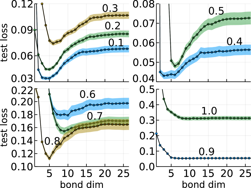
Figure 7: Inversion with subsequent tensor compression (bond dimension reduction). Test loss. Mean value and $\pm\sigma$. Averaged over $100$ data sets. $L_{2}$ regularization $10^{-6}$. Changing the MPS parameter $\varepsilon$ from $0.1$ to $1.0$ using $N_{\text{tr}}=300$ training samples.

We can see that for many values of the parameter $\varepsilon=0.1,0.2,0.3,0.5,0.6,0.7$, which controls the effect of higher order terms, the results follow the general trend discussed in the main text: the optimal bond dimension $\chi^{*}$ shifts towards higher values as the effect of higher order terms increases. However, surprisingly we find that in our case the results obtained with $\varepsilon=0.4,0.8$ do not follow this simple rule. Moreover, for $\varepsilon=0.9,1.0$ — when the data is not 1D in a sense that it cannot be efficiently modeled by an MPS (with restricted bond dimension) due to highly non-local and high-order correlations — the results of inversion and compression suggest that that the test loss monotonically decreases with bond dimension and saturates at higher bond dimension without any signature of overfitting. This is similar to our results with MNIST data set shown in top panel of Fig. IV: the test accuracy improves as bond dimension grows and then saturates, but does not degrade as bond dimension grows even further.

Figure 8 extends the results of inversion with subsequent tensor compression shown in Fig. 4, to other values of $\varepsilon$.

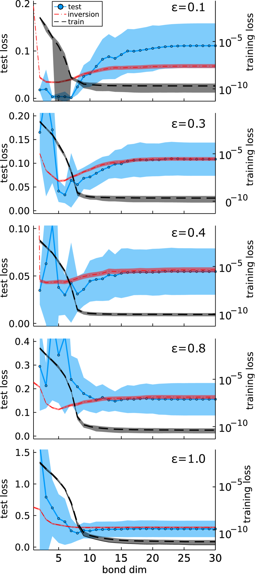
Figure 8: This figure extends the results presented in Fig. 4: it shows test (dotted blue line) and training (black dashed line) losses obtained with the DMRG optimization approach and also test loss (dot–dashed red line) obtained with the inversion and compression approach for a wider range of data complexities characterised by $\varepsilon$.

In general, we find that at large bond dimension the results of inversion and compression match optimization results well, while at smaller bond dimensions the match is more qualitative: although in most of the cases both methods result in U-shape behaviour of test loss, the actual values of test loss are notably different. At small values of $\varepsilon$, DMRG optimization generally leads to better test results at smaller bond dimensions, while it is not always true for larger $\varepsilon$.

Overall, these results support the claim that reducing bond dimension can lead to better test performance, although they also highlight the challenges and open questions associated with the effect of data properties on MPS optimization and its performance.

Appendix E Longer optimization for MNIST classification with training label noise

While the results presented in Fig. 5 do not show any evidence of double descent behavior, it is possible that running calculations much longer with label noise (randomly corrupting some portion of training labels) may reveal the second descent. Indeed, the results presented in e.g., Ref. Nakkiran et al. (2019) were obtained using a few thousands of optimization steps and also with some finite level of label noise (without noise in some cases the double descent is hardly notable and we may just overshoot it by increasing MPS bond dimension).

In Fig. 9 we show the results of calculations with MNIST using $N_{\text{tr}}=1024$ training images and $0,10,20\%$ label noise level for up $2000$ epochs (5 days of calculations, which resulted in $800-2000$ epochs depending on noise and bond dimension), for $\chi\in[2,20]$. We can see that even with noise, increasing bond dimension generally leads to better test performance and adding noise does not lead to any double descent behavior.

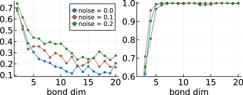
Figure 9: Model performance on MNIST. $N_{\text{tr}}=1024$ training images and $0,10,20\%$ label noise level for up $2000$ epochs. Left panel shows test error vs bond dimension at different level of label noise (the fraction of training images with randomly corrupted labels). Right panel shows training accuracy vs bond dimension.