Fixing the BMS frame of numerical relativity waveforms with BMS charges

Abstract

The Bondi-van der Burg-Metzner-Sachs (BMS) group, which uniquely describes the symmetries of asymptotic infinity and therefore of the gravitational waves that propagate there, has become increasingly important for accurate modeling of waveforms. In particular, waveform models, such as post-Newtonian (PN) expressions, numerical relativity (NR), and black hole perturbation theory, produce results that are in different BMS frames. Consequently, to build a model for the waveforms produced during the merging of compact objects, which ideally would be a hybridization of PN, NR, and black hole perturbation theory, one needs a fast and robust method for fixing the BMS freedoms. In this work, we present the first means of fixing the entire BMS freedom of NR waveforms to match the frame of either PN waveforms or black hole perturbation theory. We achieve this by finding the BMS transformations that change certain charges in a prescribed way—e.g., finding the center-of-mass transformation that maps the center-of-mass charge to a mean of zero. We find that this new method is 20 times faster, and more correct when mapping to the superrest frame, than previous methods that relied on optimization algorithms. Furthermore, in the course of developing this charge-based frame fixing method, we compute the PN expression for the Moreschi supermomentum to 3PN order without spins and 2PN order with spins. This Moreschi supermomentum is effectively equivalent to the energy flux or the null memory contribution at future null infinity $\mathscr{I}^{+}$. From this PN calculation, we also compute oscillatory ($m\not=0$ modes) and spin-dependent memory terms that have not been identified previously or have been missing from strain expressions in the post-Newtonian literature.

I Introduction

In the coming years, as gravitational wave detectors such as LIGO, Virgo, and KAGRA commence their next observing run, the catalog of astrophysical binary events is predicted to considerably increase [1, 2, 3]. With so many more gravitational-wave events, tests of Einstein’s theory of general relativity can then become even more robust and informative [4, 5]. From an analysis point of view, however, regardless of how much the gravitational-wave transient catalog increases in size over time, our ability to examine these events will always be limited by the accuracy of our waveform models, since they serve as the basis against which we can compare our observations.

Currently, and likely for the foreseeable future, the most accurate models for the gravitational waves emitted by the most commonly observed astrophysical binary system, binary black holes (BBHs), are the waveforms produced by numerical relativity (NR). Numerical waveforms uniquely maintain their precision throughout the whole evolution of the binary system. By contrast, other waveform models can only be considered correct during certain phases of the binary merger—e.g., post-Newtonian (PN) theory during inspiral or black hole perturbation theory during ringdown. However, numerical simulations are finite in time and thus can never produce the full waveform emitted by a binary event. Therefore, the best waveform model that we can hope to build is a hybridization of these models: a waveform that is PN from far into the past until we approach the merger regime, numerical throughout the merger phase, and then black hole perturbation theory during the final stages of ringdown. But, to construct such a waveform requires knowledge of how these models are related to each other. More specifically, to perform such a hybridization one needs to be able to ensure that these waveform models are in the same frame.

Like any observable in nature, the gravitational waves that we detect are emitted by a system that is in a certain frame relative to us. Often, this frame is best interpreted by using the symmetries of the system to understand the transformation between the system and the detector. For the gravitational radiation that we observe, which for practical purposes can be interpreted as existing at asymptotic infinity, the symmetry group is not the usual Poincaré group, but an extension: the BMS group [6, 7].

The BMS group is the symmetry group of asymptotically flat, Lorentzian spacetimes at null infinity $\mathscr{I}$ [6, 7]. It can be viewed as a combination of the Lorentz group with an infinite dimensional group of transformations called supertranslations [6, 7]. While surprising at first, these supertranslations have a natural origin. Consider, for example, a network of observers positioned on a sphere of finite radius encompassing a source. With some effort, these observers could combine their received signals with some understanding of their clocks’ synchronization. But, if we move these observers to asymptotic infinity, then such a synchronization becomes impossible because of the infinite separation of the observers. More specifically, they will no longer be in causal contact. Thus, we can freely time translate—i.e., supertranslate—each observer without changing the observable physics. Put differently, supertranslations are time translations applied to each point on the two-sphere at asymptotic infinity. That is, they are simply direction-dependent time translations. Consequently, supertranslations change the retarded or Bondi time $u\equiv t-r$ via

$$u^{\prime}(u,\theta,\phi) =u-\alpha(\theta,\phi)$$

$$=u-\sum\limits_{\ell=0}^{\infty}\sum\limits_{|m|\leq\ell}\alpha_{(\ell,m)}Y_{(\ell,m)}(\theta,\phi).$$ (1)

In Eq. (I), $\alpha(\theta,\phi)$ is the supertranslation parameter, with $\alpha_{\ell,m}=(-1)^{m}\overline{\alpha}_{\ell,-m}$ to make sure that the transformed Bondi time $u^{\prime}$ is real. Using spherical harmonics to express supertranslations in components is useful because we see that the usual spacetime translations are nothing more than the $\ell\leq 1$ supertranslations, while supertranslations with $\ell\geq 2$ are the new, proper supertranslations [8, 9].

When we compare waveform models, we need to make sure that the Poincaré freedoms are equivalently fixed, e.g., to ensure that both models represent a binary in the center-of-mass frame. However, because of these new symmetries that arise at asymptotic infinity through the $\ell\geq 2$ supertranslations, we must also require that the supertranslation freedom of each model is fixed in an equivalent manner. In the work of [9] this task of fixing the BMS frame of a numerical waveform to match that of a PN system was pursued for the first time. Reference [9] did this by minimizing the error between a NR strain waveform and a PN strain waveform, iterating through various BMS transformations to find the best transformations to apply to the NR system. Because the BMS group is infinite dimensional, to restrict the parameter space, Ref. [9] restricted the transformations to only include supertranslations up to $\ell\leq 4$, producing a 22-dimensional parameter space (10 Poincaré + 12 supertranslations). Because of this, the optimization algorithm required a large amount of CPU time: nearly 12 hours per system. Furthermore, because of this need to restrict the number of transformations that can be applied for the sake of the optimization algorithm, it is clear that this method of fixing the BMS frame will not be sufficient when we want to include higher order modes in our models, which will be important for future detectors.

In this work, we present a more sophisticated means of fixing the BMS frame, which relies solely on BMS charges and thus removes the need for optimization algorithms. This idea is motivated by the success that the authors of [9] had when fixing the center-of-mass frame with the center-of-mass charge. In this work, the charges used to fix the Poincaré frame are the center-of-mass charge and rotation charge, while the charge used to constrain the supertranslation freedom is a charge known as the Moreschi supermomentum, which is an extension of the usual Bondi four-momentum [10]. With these charges we then map the NR waveforms to two unique frames: the PN BMS frame, i.e., the frame that PN waveforms are in, and the superrest frame at timelike infinity $i^{+}$, i.e., the frame that quasi-normal modes (QNMs) are computed in. To map to the PN BMS frame, we find that we need to compute the PN Moreschi supermomentum to 3PN order with spins and 2PN order without spins. Upon doing so, we discover oscillatory memory terms and spin-dependent memory terms that have not been identified or have been missing from the PN strain in the literature. We find that by fixing the frame of the numerical waveforms using this charge-based method, rather than the optimization used in [9], we can not only obtain the same, if not better, errors between waveform models, but also do so in roughly 30 minutes compared to the previous run time of 12 hours.

I.1 Overview

We organize our computations and results as follows. In Sec. II we describe how the BMS transformations transform the asymptotic variables. We also present the three BMS charges that we will be using in our analyses: the center-of-mass charge, the rotation charge, and the Moreschi supermomentum. Following this, in Sec. III, we calculate the PN Moreschi supermomentum and present the new PN memory terms that have been missing from earlier calculations of the PN strain. Finally, in Sec. IV we show our numerical results. In Sec. IV.1 we outline our method for fixing the BMS frame with BMS charges. In Sec. IV.2 we compare this new charge-based method’s ability to map the NR system to either the PN BMS frame or the remnant black hole’s superrest frame to that of the previous method. In Sec. IV.3 we then highlight how waveforms produced via Cauchy-characteristic extraction are much more applicable and correct than the previously used extrapolated waveforms, once their BMS frame has been fixed with this new charge-based method. Lastly, in Appendices A and B we present the complete results of our PN calculations for the Moreschi supermomentum and the memory terms missing from the PN strain.

I.2 Conventions

We set $c=G=1$ and take $\eta_{\mu\nu}$ to be the $(-,+,+,+)$ Minkowski metric. When working with complex dyads, following the work of [11, 9], we use

$$q_{A}=-\frac{1}{\sqrt{2}}(1,i\sin\theta)\text{ and }q^{A}=-\frac{1}{\sqrt{2}}(1,i\csc\theta),$$ (2)

and write the round metric on the two-sphere $S^{2}$ as $q_{AB}$. The complex dyad obeys the following properties

$$q_{A}q^{A}=0,\quad q_{A}\bar{q}^{A}=1,\quad q_{AB}=q_{A}\bar{q}_{B}+\bar{q}_{A}q_{B}.$$ (3)

Note that this convention differs from the related works of [12, 13, 14], which in contrast do not include the $1/\sqrt{2}$ normalization factor on the dyads in Eq. (2). We choose this convention because it makes our expressions for the asymptotic charges in Eq. (17) more uniform. Nonetheless, for transparency we provide the conversion between our quantities and those of these previous works in Eq. (9).

We build spin-weighted fields with the dyads as follows. For a tensor field $W_{A\cdots D}$, the function

$$W=W_{A\cdots BC\cdots D}q^{A}\cdots q^{B}\bar{q}^{C}\cdots\bar{q}^{D}$$ (4)

with $m$ factors of $q$ and $n$ factors of $\bar{q}$ has a spin-weight of $s=m-n$. When raising and lowering spin-weights we use the Geroch-Held-Penrose differential spin-weight operators $\eth$ and $\bar{\eth}$ [15],

$$\eth W =(D_{E}W_{A\cdots BC\cdots D})q^{A}\cdots q^{B}\bar{q}^{C}\cdots\bar{q}^{D}q^{E},$$ (5a)

$$\bar{\eth}W =(D_{E}W_{A\cdots BC\cdots D})q^{A}\cdots q^{B}\bar{q}^{C}\dots\bar{q}^{D}\bar{q}^{E}.$$ (5b)

Here, $D_{A}$ is the covariant derivative on the two-sphere. The $\eth$ and $\bar{\eth}$ operators in spherical coordinates are then

$$\eth W(\theta,\phi) =-\frac{1}{\sqrt{2}}(\sin\theta)^{+s}(\partial_{\theta}+i\csc\theta\partial_{\phi})$$

$$\phantom{=.-\frac{1}{\sqrt{2}}(\sin(\theta))^{s}}\left[(\sin\theta)^{-s}W(\theta,\phi)\right],$$ (6a)

$$\bar{\eth}W(\theta,\phi) =-\frac{1}{\sqrt{2}}(\sin\theta)^{-s}(\partial_{\theta}-i\csc\theta\partial_{\phi})$$

$$\phantom{=.-\frac{1}{\sqrt{2}}(\sin(\theta))^{s}}\left[(\sin\theta)^{+s}W(\theta,\phi)\right].$$ (6b)

Thus, when acting on spin-weighted spherical harmonics, these operators produce

$$\eth(\phantom{}_{s}Y_{(\ell,m)}) =+\frac{1}{\sqrt{2}}\sqrt{(\ell-s)(\ell+s+1)}_{s+1}Y_{(\ell,m)},$$ (7a)

$$\bar{\eth}(\phantom{}_{s}Y_{(\ell,m)}) =-\frac{1}{\sqrt{2}}\sqrt{(\ell+s)(\ell-s+1)}_{s-1}Y_{(\ell,m)}.$$ (7b)

We denote the gravitational wave strain by $h$, which we represent in a spin-weight $-2$ spherical harmonic basis,

$$h(u,\theta,\phi)=\sum\limits_{\ell,m}h_{(\ell,m)}(u)\,{}_{-2}Y_{(\ell,m)}(\theta,\phi),$$ (8)

where, again, $u\equiv t-r$ is the Bondi time. We denote the Weyl scalars by $\Psi_{\text{0 -- 4}}$. The conversion from the convention of [12, 12, 14] (NR) to ours (MB) is

$$h^{\texttt{NR}}=2\bar{\sigma}^{\texttt{MB}}\quad\text{and}\quad\Psi_{i}^{\texttt{NR}}=\frac{1}{2}(-\sqrt{2})^{i}\Psi_{i}^{\texttt{MB}}.$$ (9)

Note that we will omit these superscripts and henceforth assume that everything is in the MB convention.

II BMS transformations and charges

As discussed in the introduction, the symmetry group of asymptotic infinity is not the usual Poincaré group, but the BMS group, in which the spacetime translations are extended through an infinite-dimensional group of transformations called supertranslations [6, 7]. Therefore, to understand the frame of asymptotic radiation, we must understand how the asymptotic variables transform under an arbitrary BMS transformation. Every BMS transformation can be uniquely decomposed as a pure supertranslation followed by a Lorentz transformation. In terms of retarded time $u$ and a complex stereographic coordinate $\zeta$ on the two-sphere,

$$\left(u,\zeta\right)\equiv\left(t-r,e^{i\phi}\cot\left(\theta/2\right)\right)$$ (10)

a BMS transformation acts on the coordinates as [8, 17]

$$\left(u,\zeta\right)\rightarrow\left(u^{\prime},\zeta^{\prime}\right)=\left(k\left(u-\alpha\right),\frac{a\zeta+b}{c\zeta+d}\right),$$ (11)

where the conformal factor is

$$k(\zeta,\bar{\zeta}) \equiv\frac{1+\zeta\overline{\zeta}}{\left(a\zeta+b\right)\left(\overline{a}\overline{\zeta}+\overline{b}\right)+\left(c\zeta+d\right)\left(\overline{c}\overline{\zeta}+\overline{d}\right)},$$ (12)

$(a,b,c,d)$ are complex coefficients satisfying $ad-bc=1$, and the parameter $\alpha(\zeta,\bar{\zeta})$ is a real-valued and smooth function on the celestial two-sphere. The parameters $(a,b,c,d)$ encode Lorentz transformations—both boost and rotations—whereas the function $\alpha(\zeta,\bar{\zeta})$ describes supertranslations, and thus also translations. By examining how the associated tetrad transforms under a BMS transformation [8, 22], one then finds that the shear and the Weyl scalars transform as

$$\sigma^{\prime} =\frac{e^{2i\lambda}}{k}\left[\sigma-\eth^{2}\alpha\right],$$ (13a)

$$\Psi_{A}^{\prime} =\frac{e^{\left(2-A\right)i\lambda}}{k^{3}}\sum\limits_{a=A}^{4}\begin{pmatrix}4-A\\ a-A\end{pmatrix}\left(-\frac{\eth u^{\prime}}{k}\right)^{a-A}\Psi_{a},$$ (13b)

where $A\in\{0,1,2,3,4\}$ and $\lambda$ is the spin phase [8, 22]:

$$\exp(i\lambda)=\left[\frac{\partial\overline{\zeta^{\prime}}}{\partial\overline{\zeta}}\left(\frac{\partial\zeta^{\prime}}{\partial\zeta}\right)^{-1}\right]^{1/2}=\frac{c\zeta+d}{\overline{c}\overline{\zeta}+\overline{d}}.$$ (14)

For a Lorentz transformation parameterized by $(a,b,c,d)$ and a supertranslation parameterized by $\alpha$, Eqs. (11) and (13) are the primary ingredients for understanding how the asymptotic variables, namely the shear as well as the Weyl scalars, transform under a BMS transformation. All that remains is a method for finding the necessary frame-fixing BMS transformation, which we outline in Secs. II.1 for the Poincaré transformations and II.2 for the proper supertranslations.

II.1 Poincaré charges

In this section, following the work of [9], we outline the Poincaré charges that will be used to completely fix the Poincaré transformation freedom of the asymptotic shear and Weyl scalars. As was shown in [6, 23, 24, 25, 26, 27, 28, 29, 30, 9], by examining the expansion of the Bondi-Sachs metric near future null infinity, one can identify certain functions that yield the Poincaré charges when integrated over the celestial two-sphere. They are the Bondi mass aspect $m$, the Lorentz aspect $N$, and the energy moment aspect $E$, which in the MB convention are

$$m(u,\theta,\phi) \equiv-\text{Re}\left[\Psi_{2}+\sigma\dot{\bar{\sigma}}\right],$$ (15a)

$$N(u,\theta,\phi) \equiv-\left(\Psi_{1}+\sigma\eth\bar{\sigma}+u\eth m+\frac{1}{2}\eth\left(\sigma\bar{\sigma}\right)\right),$$ (15b)

$$E(u,\theta,\phi) \equiv N+u\eth m$$

$$=-\left(\Psi_{1}+\sigma\eth\bar{\sigma}+\frac{1}{2}\eth\left(\sigma\bar{\sigma}\right)\right).$$ (15c)

Thus, by defining a collection of spin-0 scalar functions, $\mathbf{n}(\theta,\phi)$, whose components are unique combinations of the $\ell\leq 1$ spherical harmonics so as to represent one of the four Cartesian coordinates $t$, $x$, $y$, or $z$, i.e.,

$$n^{t} =1$$

$$=\sqrt{4\pi}Y_{(0,0)},$$ (16a)

$$n^{x} =\sin\theta\cos\phi,$$

$$=\sqrt{\frac{4\pi}{3}}\left[\frac{1}{\sqrt{2}}\left(Y_{(1,-1)}-Y_{(1,+1)}\right)\right],$$ (16b)

$$n^{y} =\sin\theta\sin\phi$$

$$=\sqrt{\frac{4\pi}{3}}\left[\frac{i}{\sqrt{2}}\left(Y_{(1,-1)}+Y_{(1,+1)}\right)\right],$$ (16c)

$$n^{z} =\cos\theta$$

$$=\sqrt{\frac{4\pi}{3}}Y_{(1,0)},$$ (16d)

we can then compute each Cartesian component of the translation, rotation, boost, and center-of-mass charges. For $a\in\{t,x,y,z\}$, these four Poincaré charges are

$$P^{a}(u) =\frac{1}{4\pi}\int_{S^{2}}n^{a}m\,d\Omega,$$ (17a)

$$J^{a}(u) =\frac{1}{4\pi}\int_{S^{2}}\text{Re}\left[\left(\bar{\eth}n^{a}\right)\left(-iN\right)\right]\,d\Omega,$$ (17b)

$$K^{a}(u) =\frac{1}{4\pi}\int_{S^{2}}\text{Re}\left[\left(\bar{\eth}n^{a}\right)N\right]\,d\Omega,$$ (17c)

$$G^{a}(u) =\left(K^{a}+uP^{a}\right)/P^{t}$$

$$=\frac{1}{4\pi}\int_{S^{2}}\text{Re}\left[\left(\bar{\eth}n^{a}\right)\left(N+u\eth m\right)\right]\,d\Omega/P^{t}.$$ (17d)

Then, by making use of the orthogonality property of spherical harmonics, we find that the four vector of a Poincaré charge $\Pi$ is simply

$$\Pi^{t} =\frac{1}{\sqrt{4\pi}}\Pi_{(0,0)},$$ (18a)

$$\Pi^{x} =\frac{1}{\sqrt{4\pi}}\frac{1}{\sqrt{6}}\text{Re}\left[\Pi_{(1,-1)}-\Pi_{(1,+1)}\right],$$ (18b)

$$\Pi^{y} =\frac{1}{\sqrt{4\pi}}\frac{1}{\sqrt{6}}\text{Im}\left[\Pi_{(1,-1)}+\Pi_{(1,+1)}\right],$$ (18c)

$$\Pi^{z} =\frac{1}{\sqrt{4\pi}}\frac{1}{\sqrt{3}}\text{Re}\left[\Pi_{(1,0)}\right],$$ (18d)

where $\Pi_{(\ell,m)}$ is the $(\ell,m)$ mode of the charge $\Pi$ in the basis of spin-$s$ spherical harmonics ($s=0$ for $m$, and $s=1$ for $-iN,N$, and $N+u\eth m$). These charges in Eqs. (17) have simple interpretations by analogy to kinematics in Minkowski space. $P^{a}$ is the total linear momentum, $J^{a}$ is the total angular momentum—orbital plus spin, $K^{a}$ is proportional to the center-of-mass at time $u=0$, and $G^{a}$ is the center-of-mass at time $u$. For more on these charges in the PN formulation, see [31] for an analysis using conservative point particle theory, [32] for an analysis when radiation is involved, and [33] for a connection to the Poincaré and BMS flux-balance laws.

While the Poincaré charges in Eq. (17) are the most natural to work with for fixing frames, since we will be comparing the frame of numerical waveforms to that of PN waveforms, we need either PN or BH perturbation theory expressions for these charges. Notice, however, that Eqs. (17) contain the Weyl scalars $\Psi_{1}$ and $\Psi_{2}$. Thus we need the PN expressions for these Weyl scalars, which have not been computed thus far in the PN literature. Fortunately, PN waveforms are inherently constructed in the center-of-mass frame. The center-of-mass charge $G^{a}$, given in Eq. (17), can be taken to have an average of zero, i.e., an intercept and a slope of zero when fitted to with a linear function in time, though it is oscillatory at high enough PN order. For mapping to the superrest frame, we can also map the center-of-mass charge to have an average of zero, seeing as we want our remnant black hole to asymptote to a stationary Kerr black hole.

The rotation charge, Eq. (17b), however, tends to be some nontrivial function of time. Therefore, for fixing the rotation freedom to match that of PN waveforms, we require an alternative rotation charge that is independent of the $\Psi_{1}$ and $\Psi_{2}$ Weyl scalars. In the work of [20] such a rotation charge was built by finding the angular velocity which keeps the radiative fields as constant as possible in the corotating frame. Following the notation of [20, 34], this vector, with “$\cdot$” the usual dot product, is

$$\vec{\omega}(u)=-\langle\vec{L}\vec{L}\rangle^{-1}\cdot\langle\vec{L}\partial_{t}\rangle,$$ (19)

where we use the $u$-dependent vector and matrix

$$\langle\vec{L}\partial_{t}\rangle^{a} \equiv\sum\limits_{\ell,m,m^{\prime}}\text{Im}\left[\bar{f}_{(\ell,m^{\prime})}\langle\ell,m^{\prime}|L^{a}|\ell,m\rangle\dot{f}_{(\ell,m)}\right],$$ (20a)

$$\langle\vec{L}\vec{L}\rangle^{ab} \equiv\sum\limits_{\ell,m,m^{\prime}}\bar{f}_{(\ell,m^{\prime})}\langle\ell,m^{\prime}|L^{(a}L^{b)}|\ell,m\rangle f_{(\ell,m)},$$ (20b)

and $f(u,\theta,\phi)$ is some function that corresponds to the asymptotic radiation, e.g., the shear $\sigma$ or the news $\dot{\sigma}$. This data is represented in the basis $|\ell,m\rangle$ of spin-weighted spherical harmonics, with time-dependent mode weights $f_{(\ell,m)}$, i.e. $|f\rangle=\sum_{\ell,m}f_{(\ell,m)}|\ell,m\rangle$. The operator $\vec{L}$ is the infinitesimal generator of rotations, whose related charge is the total angular momentum charge $J^{a}$ provided in Eq. (17b). Therefore, when fixing the frame of the waveforms to match that of the PN system, i.e., to match the frames at spacelike infinity, we will use the vector in Eq. (19).

For fixing the rotation at timelike infinity—the case of a system consisting of a single black hole—we also choose to use a rotation charge that is not the charge seen in Eq. (17b). This is because at timelike infinity, provided that we are in the center-of-mass frame of the remnant black hole, we do not expect there to be any orbital angular momentum contributions, but instead only spin angular momentum contributions. Thus, for fixing the rotation freedom it is more useful to work with the asymptotic dimensionless spin vector [11]:

$$\vec{\chi}(u)=\frac{\gamma}{M_{\text{B}}^{2}}\left(\vec{J}+\vec{v}\times\vec{K}\right)-\frac{\gamma-1}{M_{\text{B}}^{2}}\left(\hat{v}\cdot\vec{J}\right)\hat{v},$$ (21)

where

$$\gamma(u)\equiv\sqrt{1-\left|\vec{v}\right|^{2}}^{-1}$$ (22)

is the Lorentz factor,

$$M_{\text{B}}(u)\equiv\sqrt{-\eta_{\mu\nu}P^{\mu}P^{\nu}}$$ (23)

is the Bondi mass,

$$\vec{v}(u)\equiv\vec{P}/P^{t}$$ (24)

is the velocity vector, and the vectors $\vec{J}$ and $\vec{K}$ are the angular momentum and boost Poincaré charges, i.e., Eqs. (17b) and (17c), evaluated at the vector $\vec{n}=\left(\vec{x},\vec{y},\vec{z}\right)$. With this charge, we can then fix the rotation freedom by solving for the rotation that maps this charge to be parallel to the positive $z$-axis: the standard convention for studying QNMs. This fully fixes the rotation freedom of our system, up to a $U(1)$ transformation that can be thought of as a constant phase change. For mapping to the PN BMS frame, this remaining $U(1)$ freedom is fixed while running a time and phase alignment that minimizes the residual between the NR and PN strain waveforms. For mapping to the superrest frame at timelike infinity, no phase fixing is performed as it is not necessary for analyzing QNMs.

II.2 $\ell\geq 2$ supertranslation charge

For fixing the supertranslation freedom of a system, because the supertranslations are just extensions of the usual spacetime translations, it is reasonable to ask if there is a clear extension of the Bondi four-momentum [6]

$$P^{a}(u)=\frac{1}{4\pi}\int_{S^{2}}n^{a}\text{Re}\left[\Psi_{2}+\sigma\dot{\bar{\sigma}}\right]\,d\Omega.$$ (25)

As was pointed out by Dray and Streubel [35], and also independently realized later by Wald and Zoupas [36], the possible choices for a supermomentum can be written as

$$\Psi_{p,q}(u,\theta,\phi)=\Psi_{2}+\sigma\dot{\bar{\sigma}}+p\left(\eth^{2}\bar{\sigma}\right)-q\left(\bar{\eth}^{2}\sigma\right),$$ (26)

where $p$ and $q$ are arbitrary real numbers. From this supermomentum expression, one can show that if $p=q$ then there is no supermomentum flux in Minkowski space and if $p+q=1$ then the supermomentum is real [35, 36]. This leads to a natural choice of supermomentum being the Geroch (G) supermomentum with $p=q=\frac{1}{2}$, i.e.,

$$\Psi_{\text{G}}(u,\theta,\phi)\equiv\Psi_{2}+\sigma\dot{\bar{\sigma}}+\frac{1}{2}\left(\eth^{2}\bar{\sigma}-\bar{\eth}^{2}\sigma\right).$$ (27)

It turns out, though, that in regimes that are nonradiative (i.e., $\dot{\sigma}=0$), the Geroch supermomentum is not changed by a supertranslation since

$$\Psi_{\text{G}}^{\prime} =\frac{1}{k^{3}}\left(\Psi_{\text{G}}-\frac{1}{2}\left[2\eth\alpha\eth\dot{\bar{\sigma}}+\left(\eth^{2}\alpha\right)\dot{\bar{\sigma}}+(\eth\alpha)^{2}\ddot{\bar{\sigma}}+\text{c.c.}\right]\right)$$

$$\rightarrow\frac{1}{k^{3}}\Psi_{\text{G}}\quad\left(\text{for }\dot{\sigma}\rightarrow 0\right).$$ (28)

Therefore, while the Geroch supermomentum may be an ideal choice for a physical supermomentum, for fixing the supertranslation freedom of our system it will instead be useful to construct a supertranslation charge that does transform under supertranslations. But what are the features of the system that we would like to control using these supertranslation transformations?

When we examine how supertranslations transform asymptotic radiation, Eq. (13a) shows that the shear is changed by a term constant in time and proportional to the supertranslation parameter $\alpha(\theta,\phi)$. Consequently, because supertranslations affect the value of the shear even in nonradiative regimes, we can interpret them as also being related to the gravitational memory effect—i.e., the physical observable that corresponds to the permanent net change in the metric due to the passage of transient gravitational radiation [37, 38, 39].

Gravitational memory can best be understood through the supermomentum balance law [43], which says that the real part of the shear can be written as

$$\text{Re}\left[\bar{\eth}^{2}\sigma\right] =m+\int_{-\infty}^{u}|\dot{\sigma}|^{2}du+\left(\text{Re}\left[\bar{\eth}^{2}\sigma\right]-m\right)|^{-\infty}$$

$$=m+\mathcal{E}-M_{\text{ADM}},$$ (29)

where

$$\mathcal{E}(u,\theta,\phi)\equiv\int_{-\infty}^{u}|\dot{\sigma}|^{2}du$$ (30)

is proportional to the energy radiated up to time $u$ into the direction $(\theta,\phi)$, and $M_{\text{ADM}}$ is the Arnowitt-Deser-Misner (ADM) mass [44]. If one evaluates this equation between early times and late times (i.e., $\pm\infty$), then the net change in the shear (the memory) has two unique contributions: one from the net change in the mass aspect (the ordinary memory) and one from the net change in the system’s energy flux (the null memory). Note that the ADM mass does not contribute to the memory because it is a constant on the two-sphere and therefore has no $\ell\geq 2$ components. Typically, ordinary memory occurs in systems that have unbound masses, such as hyperbolic black holes, while null memory occurs in systems that have bound masses, such as binary black holes. Furthermore, if one examines how this equation changes under a BMS transformation, one finds

$$m^{\prime} =\frac{1}{k^{3}}\left(m+\frac{1}{2}\left[2\eth\alpha\eth\dot{\bar{\sigma}}+\left(\eth^{2}\alpha\right)\dot{\bar{\sigma}}+(\eth\alpha)^{2}\ddot{\bar{\sigma}}+\text{c.c.}\right]\right)$$

$$\rightarrow\frac{1}{k^{3}}m\quad\left(\text{when nonradiative}\right),$$ (31a)

$$\mathcal{E}^{\prime} =\frac{1}{k^{3}}\left(\mathcal{E}-\eth^{2}\bar{\eth}^{2}\alpha\right)\quad\left(\text{always}\right).$$ (31b)

So, when written in terms of its charge ($m$) and flux ($\mathcal{E}$) contributions, the only part of the shear that transforms under a supertranslation in nonradiative regimes of $\mathscr{I}^{+}$ is the energy flux contribution. This suggests that the charge that would be the ideal charge for measuring what supertranslation we should apply to our system would be something equivalent to the energy flux. Fortunately, such a charge, the Moreschi supermomentum, has already been examined by Dain and Moreschi [22, 10, 17, 18]:

$$\Psi_{\text{M}}(u,\theta,\phi) \equiv\Psi_{2}+\sigma\dot{\bar{\sigma}}+\eth^{2}\bar{\sigma}.$$ (32)

This is simply Eq. (26) with coefficients $p=1$ and $q=0$. By rewriting the first term in Eq. (32) as a time integral, making use of the Bianchi identity

$$\dot{\Psi}_{2}=-\sigma\ddot{\bar{\sigma}}+\eth^{2}\bar{\sigma},$$ (33)

and integrating by parts we find

$$\Psi_{\text{M}} =\left(\int_{-\infty}^{u}\dot{\Psi}_{2}\,du-M_{\text{ADM}}\right)+\sigma\dot{\bar{\sigma}}+\eth^{2}\bar{\sigma}$$

$$=\left(\int_{-\infty}^{u}\left(-\sigma\ddot{\bar{\sigma}}+\eth^{2}\bar{\sigma}\right)du-M_{\text{ADM}}\right)+\sigma\dot{\bar{\sigma}}+\eth^{2}\bar{\sigma}$$

$$=\int_{-\infty}^{u}|\dot{\sigma}|^{2}du-M_{\text{ADM}}$$

$$=\mathcal{E}-M_{\text{ADM}}.$$ (34)

Because of this, the Moreschi supermomentum can also be thought of as the memory part of the mass moment. Furthermore, by using Eq. (31b) with Eq. (II.2), one finds that the Moreschi supermomentum transforms as

$$\Psi_{\text{M}}^{\prime}=\frac{1}{k^{3}}\left(\Psi_{\text{M}}-\eth^{2}\bar{\eth}^{2}\alpha\right).$$ (35)

Equations (II.2) and (35) then imply that we can rewrite the transformation of the shear under a supertranslation in a nonradiative regime of $\mathscr{I}^{+}$ as

$$\text{Re}\left[\bar{\eth}^{2}\sigma\right]^{\prime} =m^{\prime}+\Psi_{\text{M}}^{\prime}$$

$$=m+\left(\Psi_{\text{M}}-\eth^{2}\bar{\eth}^{2}\alpha\right).$$ (36)

This shows that by fixing the supertranslation freedom with the Moreschi supermomentum one also immediately has an understanding of how the shear will transform. Consider applying the supertranslation that maps the $\ell\geq 1$, i.e., the nontemporal, components of $\Psi_{\text{M}}$ to zero in a nonradiative regime of $\mathscr{I}^{+}$. For bound systems, which asymptote to regimes of $\mathscr{I}^{+}$ that are nonradiative and stationary, such a transformation also maps the shear to zero in the nonradiative regime of $\mathscr{I}^{+}$ because in this regime $\text{Re}\left[\bar{\eth}^{2}\sigma\right]=\Psi_{\text{M}}$. Consequently, for systems like BBHs, by performing such a mapping at $u\rightarrow-\infty$ or at $u\rightarrow+\infty$, one can wholly fix the supertranslation freedom of the system so that it agrees with PN waveforms or QNM models. Moreschi calls a frame in which the $\ell\geq 1$ components of $\Psi_{\text{M}}$ are zero a nice section of $\mathscr{I}^{+}$; we, like [9, 46], will instead call it the superrest frame. Furthermore, since $\Psi_{\text{M}}$ in the superrest frame at $u\rightarrow\pm\infty$ is equal to Bondi mass $M_{\text{B}}$, the supertranslation $\alpha$ that maps to the superrest frame at a single time can be computed with relative ease via the implicit equation

$$\eth^{2}\bar{\eth}^{2}\alpha=\Psi_{\text{M}}(u=\alpha,\theta,\phi)+k_{\text{rest}}(\alpha,\theta,\phi)^{3}M_{\text{B}}(\alpha).$$ (37)

This equation for $\alpha$ is obtained by taking $\Psi_{\text{M}}^{\prime}=M_{\text{B}}$ in Eq. (35) and rearranging terms. Note that here the conformal factor on the right, $k_{\text{rest}}$, is a special case of the conformal factor given in Eq. (12): namely the one coming from a boost to the instantaneous rest frame at some fixed time, computed via

$$k_{\text{rest}}(u,\theta,\phi)\equiv\frac{1}{\gamma\left(1-\vec{v}\cdot\vec{r}\right)}=\frac{M_{B}}{P_{a}n^{a}}.$$ (38)

Apart from this, Dain and Moreschi also proved that, provided a certain condition on the energy flux, which is always obeyed by nonradiative regimes of $\mathscr{I}^{+}$, this equation always has a regular solution [18]. Therefore, for the frames that we are mapping to, such a supertranslation will always exist. Furthermore, Dain and Moreschi also showed that Eq. (37) can be solved iteratively. That is, if one wishes to find the supertranslation that maps the system to the superrest frame at time $u_{0}$, they can take Eq. (37) and evaluate the right-hand side at time $u=u_{0}$, solve for $\alpha$, evaluate the right-hand side at time $u=\alpha$, solve for a new $\alpha$, etc., until $\alpha$ converges to a solution. We will make use of this fact in Sec. IV.

What remains unclear at this point, however, is whether the Moreschi supermomentum is also the right charge to use for fixing the frame of systems with unbound masses. For these unbound systems, the $\ell\geq 2$ components of $m$ can have a nonzero net change between $u\rightarrow\pm\infty$, which means that mapping the $\ell\geq 1$ components of $\Psi_{\text{M}}$ to zero need not map the system to a shear-free section of $\mathscr{I}^{+}$. Despite this, it may be that shear-free sections are not necessarily that meaningful and really what one should strive for when fixing the supertranslation freedom is ensuring that the shear has only hard contributions [24], i.e., no contribution from the energy flux. In this work, however, because we focus on bound systems, like BBHs and perturbed BHs, it will suffice to only consider the Moreschi supermomentum as the charge for fixing the supertranslation freedom of our systems.

III PN supermomentum

With the Moreschi supermomentum now identified as the supertranslation charge that can map BBH systems (or other bound systems) to shear-free sections of $\mathscr{I}^{+}$, there are two obvious BMS frames that one can map to: the superrest frame at either $u\rightarrow-\infty$ or $u\rightarrow+\infty$. The first choice can be understood as mapping the system to the same frame as PN waveforms, i.e., shear-free in the infinite past. The second is naturally understood as mapping to the superrest frame of the remnant BH, i.e., making the metric equivalent to the Kerr metric rather than a supertranslated Kerr metric [47]. Waveforms produced by numerical relativity, however, are finite in time and thus do not contain information about $u\rightarrow-\infty$ or $u\rightarrow+\infty$. Thus, for fixing the frame of these waveforms we need to know what we should be mapping the numerical Moreschi supermomentum to with the Bondi times that we have access to. For mapping to the superrest frame of the remnant BH ($u\rightarrow+\infty$), this is simple because the radiation decays fast enough that mapping at or near the end of the simulation is a reasonable approximation to $u\rightarrow+\infty$. For mapping to the same frame as PN waveforms, however, we cannot rely on approximations because the radiation during the inspiral of a BBH merger cannot be considered negligible. We instead need to know the Moreschi supermomentum predicted by PN theory. This will allow us to map the numerical supermomentum to equal that of the PN system, which serves as a proxy for mapping our NR system to the superrest frame at spacelike infinity. Accordingly, we now perform a PN calculation of the Moreschi supermomentum.

III.1 PN Moreschi supermomentum

The main ingredients for this PN calculation are the PN expressions for the strain both with and without the BH spins [48, 45, 21, 49], the orbital energy [48, 50, 51], and the luminosity [48, 50, 51]. Using Eq. (9) to replace the shear by the strain in Eq. (II.2) and then moving the ADM mass to the other side of the equation yields

$$\Psi_{\text{M}}+M_{\text{ADM}}=\int_{-\infty}^{u}|\dot{\sigma}|^{2}du=\frac{1}{4}\int_{-\infty}^{u}|\dot{h}|^{2}du,$$ (39)

Therefore, provided a spherical harmonic decomposition of the PN strain, any spherical harmonic mode of the supermomentum can be computed by integrating the product of various spin-weighted spherical harmonics over the two-sphere as well as integrating the products of various modes of the strain with respect to time:

$$\Psi_{\text{M}}^{(\ell,m)} =\frac{1}{4}\sum\limits_{\ell_{1},|m_{1}|\leq\ell_{1}}\sum\limits_{\ell_{2},|m_{2}|\leq\ell_{2}}$$

$$\phantom{=.}\left[\int_{S^{2}}\overline{\phantom{}{}_{0}Y_{\ell,m}}\,\overline{\phantom{}{}_{-2}Y_{\ell_{1},m_{1}}}\,\phantom{}_{-2}Y_{\ell_{2},m_{2}}d\Omega\right]$$

$$\phantom{=.}\left[\int\overline{\dot{h}^{(\ell_{1},m_{1})}}\,\dot{h}^{(\ell_{2},m_{2})}du\right].$$ (40)

The first of these integrals can be easily computed from the spin-weighted spherical harmonics’ relationship to the Wigner $D$-matrices combined with the known integral of a product of three $D$ matrices [52], which produces

$$\int_{S^{2}}\phantom{}{}_{s_{1}}Y_{\ell_{1}m_{1}}\,\phantom{}{}_{s_{2}}Y_{\ell_{2}m_{2}}\,\phantom{}{}_{s_{3}}Y_{\ell_{3}m_{3}}d\Omega=\sqrt{\frac{(2\ell_{1}+1)(2\ell_{2}+1)(2\ell_{3}+1)}{4\pi}}\begin{pmatrix}\ell_{1}&\ell_{2}&\ell_{3}\\ m_{1}&m_{2}&m_{3}\end{pmatrix}\begin{pmatrix}\ell_{1}&\ell_{2}&\ell_{3}\\ -s_{1}&-s_{2}&-s_{3}\end{pmatrix}.$$ (41)

For this part of the calculation, we also need the identity

$$\overline{\phantom{}{}_{s}Y_{\ell,m}}=(-1)^{s+m}\phantom{}_{-s}Y_{\ell,-m}.$$ (42)

Next consider the integral with respect to time in the final part of Eq. (40). Because any mode of the strain can be written as

$$h^{(\ell,m)}=\frac{2M\nu x}{R}\sqrt{\frac{16\pi}{5}}\mathcal{H}^{(\ell,m)}e^{-im\psi},$$ (43)

where $M\equiv m_{1}+m_{2}$, $\nu\equiv m_{1}m_{2}/M^{2}$, $x\equiv(M\omega)^{2/3}$ is the usual PN parameter, $\psi$ is the auxiliary phase variable (see Eq. (321) of [48]), and $\mathcal{H}^{(\ell,m)}$ is a polynomial in $x$, we can perform a change of coordinates from $u$ to $x$ to obtain a series of integrals of the form

$$\int_{x_{0}}^{x}\dot{x}\left(d\psi/dx\right)^{a}x^{b}e^{-iA\psi(x)}dx,$$ (44)

where $a\in\{0,1,2\}$, $b\in\mathbb{N}$, $A\in\mathbb{Z}$, and $x_{0}$ corresponds to an arbitrary initial frequency $\omega_{0}$. To evaluate these various integrals over $x$, consider first integrating the following expression by parts to obtain

$$\int_{x_{0}}^{x}f(x)e^{\varphi(x)}dx=$$

$$\left[\left(\frac{d\varphi}{dx}\right)^{-1}fe^{\varphi}\right]_{x_{0}}^{x}$$

$$-\int_{x_{0}}^{x}\left[\left(\frac{d\varphi}{dx}\right)^{-1}\frac{df}{dx}-\left(\frac{d\varphi}{dx}\right)^{-2}\frac{d^{2}\varphi}{dx^{2}}f\right]e^{\varphi}dx.$$ (45)

Because $\varphi\propto\psi\sim x^{-5/2}$, the PN order of the integrand on the right-hand side ends up being 2.5PN higher than the original integrand. Thus we can evaluate these integrals by integrating by parts until the unevaluated integrals have been pushed to a PN order above what we consider. Alternatively, one can evaluate such integrals with either the stationary phase approximation or the method of steepest descent [53], but the result should be the same. By carrying out this integration procedure, we then find that we can compute the PN Moreschi supermomentum to relative 3PN order when spins are not included and relative 2PN order when spins are included, with the limiting factor being the available PN order of the strain that we input into Eq. (39). We write the modes of the Moreschi supermomentum as

$$\Psi_{\text{M}}^{(\ell,m)}=\frac{2M\nu x}{R^{2}}\sqrt{\frac{\pi}{4}}\mathcal{P}^{(\ell,m)}e^{-im\psi}-M\delta_{\ell,0}\delta_{m,0}$$ (46)

where $\mathcal{P}^{(\ell,m)}$ is a polynomial in $x$. The term in $M$ that arises when $(\ell,m)=(0,0)$ is because of the presence of the ADM mass in Eq. (II.2). While we write our results in full in Appendices A and B, we provide a few of the most interesting modes below. These results have been obtained using Mathematica.

$$\mathcal{P}^{(0,0)} =1+x\left(-\frac{3}{4}-\frac{\nu}{12}\right)+x^{2}\left(-\frac{27}{8}+\frac{19\nu}{8}-\frac{\nu^{2}}{24}\right)+x^{3}\left(-\frac{675}{64}+\left(\frac{34445}{576}-\frac{205\pi^{2}}{96}\right)\nu-\frac{155\nu^{2}}{96}-\frac{35\nu^{3}}{5184}\right),$$ (47a)

$$\mathcal{P}_{\text{spin}}^{(0,0)} =x^{3/2}\left(\frac{14S_{\ell}}{3M^{2}}+\frac{2\delta\Sigma_{\ell}}{M^{2}}\right)$$

$$\phantom{=.}+x^{2}\left(-\frac{16\vec{S}\cdot\vec{S}+3\vec{\Sigma}\cdot\vec{\Sigma}+32S_{\ell}^{2}+9\Sigma_{\ell}^{2}}{12M^{4}}-\frac{4\delta\left(\vec{S}\cdot\vec{\Sigma}+2S_{\ell}\Sigma_{\ell}\right)}{3M^{4}}+\frac{4\left(\vec{\Sigma}\cdot\vec{\Sigma}+2\Sigma_{\ell}^{2}\right)\nu}{3M^{4}}\right),$$ (47b)

$$\mathcal{P}^{(1,1)} =\frac{43}{70}\sqrt{\frac{3}{2}}\Bigg{\{}x^{3}\left(\frac{1856\delta\nu}{129}\right)\Bigg{\}},$$ (47c)

$$\mathcal{P}_{\text{spin}}^{(1,1)} =0,$$ (47d)

$$\mathcal{P}^{(2,0)} =\frac{2}{7}\sqrt{5}\Bigg{\{}1+x\left(-\frac{4075}{4032}+\frac{67\nu}{48}\right)+x^{2}\left(-\frac{151877213}{67060224}-\frac{123815\nu}{44352}+\frac{205\nu^{2}}{352}\right)+\pi x^{5/2}\left(-\frac{253}{336}+\frac{253\nu}{84}\right)$$

$$\phantom{=.\frac{2}{7}\sqrt{5}\Bigg{\{}}+x^{3}\left(-\frac{4397711103307}{532580106240}+\left(\frac{700464542023}{13948526592}-\frac{205\pi^{2}}{96}\right)\nu+\frac{69527951\nu^{2}}{166053888}+\frac{1321981\nu^{3}}{5930496}\right)\Bigg{\}},$$ (47e)

$$\mathcal{P}_{\text{spin}}^{(2,0)} =\frac{2}{7}\sqrt{5}\Bigg{\{}x^{3/2}\left(\frac{16S_{\ell}}{3M^{2}}+\frac{419\delta\Sigma_{\ell}}{160M^{2}}\right)$$

$$\phantom{=.\frac{2}{7}\sqrt{5}\Bigg{\{}}+x^{2}\left(-\frac{128\vec{S}\cdot\vec{S}+24\vec{\Sigma}\cdot\vec{\Sigma}+256S_{\ell}^{2}+75\Sigma_{\ell}^{2}}{96M^{4}}-\frac{4\delta\left(\vec{S}\cdot\vec{\Sigma}+2S_{\ell}\Sigma_{\ell}\right)}{3M^{4}}+\frac{4\left(\vec{\Sigma}\cdot\vec{\Sigma}+2\Sigma_{\ell}^{2}\right)\nu}{3M^{4}}\right)\Bigg{\}},$$ (47f)

$$\mathcal{P}^{(3,1)} =\frac{223}{120\sqrt{21}}\Bigg{\{}x^{3}\left(\frac{3872\delta\nu}{223}\right)\Bigg{\}},$$ (47g)

$$\mathcal{P}_{\text{spin}}^{(3,1)} =0.$$ (47h)

Name	CCE radius	$q$	$\chi_{A}$:	$(\hat{x},\,$	$\hat{y},\,$	$\hat{z})$	$\chi_{B}$:	$(\hat{x},\,$	$\hat{y},\,$	$\hat{z})$
q1_nospin	292	$1.0$		$(0,\,$	$0,\,$	$0)$		$(0,\,$	$0,\,$	$0)$
q1_aligned_chi0_2	261	$1.0$		$(0,\,$	$0,\,$	$0.2)$		$(0,\,$	$0,\,$	$0.2)$
q1_aligned_chi0_4	250	$1.0$		$(0,\,$	$0,\,$	$0.4)$		$(0,\,$	$0,\,$	$0.4)$
q1_aligned_chi0_6	236	$1.0$		$(0,\,$	$0,\,$	$0.6)$		$(0,\,$	$0,\,$	$0.6)$
q1_antialigned_chi0_2	274	$1.0$		$(0,\,$	$0,\,$	$0.2)$		$(0,\,$	$0,\,$	$-0.2)$
q1_antialigned_chi0_4	273	$1.0$		$(0,\,$	$0,\,$	$0.4)$		$(0,\,$	$0,\,$	$-0.4)$
q1_antialigned_chi0_6	270	$1.0$		$(0,\,$	$0,\,$	$0.6)$		$(0,\,$	$0,\,$	$-0.6)$
q1_precessing	305	$1.0$		$(0.487,\,$	$0.125,\,$	$-0.327)$		$(-0.190,\,$	$0.051,\,$	$-0.227)$
q1_superkick	270	$1.0$		$(0.6,\,$	$0,\,$	$0)$		$(-0.6,\,$	$0,\,$	$0)$
q4_nospin	235	$4.0$		$(0,\,$	$0,\,$	$0)$		$(0,\,$	$0,\,$	$0)$
q4_aligned_chi0_4	222	$4.0$		$(0,\,$	$0,\,$	$0.4)$		$(0,\,$	$0,\,$	$0.4)$
q4_antialigned_chi0_4	223	$4.0$		$(0,\,$	$0,\,$	$0.4)$		$(0,\,$	$0,\,$	$-0.4)$
q4_precessing	237	$4.0$		$(0.487,\,$	$0.125,\,$	$-0.327)$		$(-0.190,\,$	$0.051,\,$	$-0.227)$
SXS:BBH:0305 (GW150914)	267	$1.221$		$(0,\,$	$0,\,$	$0.330)$		$(0,\,$	$0,\,$	$-0.440)$

Table 1: Parameters of the BBH mergers used in our results. The mass ratio is $q=M_{A}/M_{B}$ and the initial dimensionless spins of the two black holes are $\chi_{A}$ and $\chi_{B}$. These simulations have been made publicly available at [54, 55].

For the terms in these expressions that include spins, with $M_{1}$ and $M_{2}$ and $\vec{S}_{1}$ and $\vec{S}_{2}$ the masses and spins of the two black holes,

$$\vec{S}\equiv\vec{S}_{1}+\vec{S}_{2}$$ (48)

is the total spin vector,

$$\vec{\Sigma}\equiv M\left(\frac{\vec{S}_{2}}{M_{2}}-\frac{\vec{S}_{1}}{M_{1}}\right)$$ (49)

can be viewed as an effective antisymmetric spin vector, $\delta\equiv\left(M_{1}-M_{2}\right)/M$, $\hat{n}$ is the unit vector pointing from black hole $2$ to black hole $1$, $\hat{\lambda}$ is the unit vector in the direction of $d\hat{n}/du$, and $\hat{\ell}=\hat{n}\times\hat{\lambda}$. We include these modes here for the following reasons. The $(0,0)$ mode is proportional to the energy radiated to future null infinity, and matches the orbital energy results of [48, 50, 51, 56] to 3PN order without spins and also to 2PN order with spins. The $(1,1)$ mode corresponds to the radiated momentum and therefore highlights that at 3PN order without spins the center-of-mass is not stationary but oscillates about the origin. When spins are not included, the expression for the $(2,0)$ mode, which is the main memory mode, recovers the previous PN memory result of [45]. But, when spins are included, we observe new memory terms that are proportional to spin. This is a new result in PN theory, even though this behavior has been known in the numerical community [57, 12]. Last, the $(3,1)$ mode highlights a new identification in post-Newtonian theory, namely the existence of oscillatory memory modes, which arise at 3PN order and have been known to exist but have not been computed in a memory context, even though the 3PN strain without spins is complete [45, 58].

IV Numerical analysis

With the charges needed for fixing the BMS frame summarized in Sec. II, we now present numerical results of mapping BBH waveforms to either the PN BMS frame or the superrest frame of the remnant black hole at $i^{+}$. We numerically evolved a set of 14 binary black hole mergers with varying mass ratios and spin configurations using the spectral Einstein code (SpEC) [59]. We list the important parameters of these various BBH systems in Table 1. Each simulation contains roughly 19 orbits prior to merger and is evolved until the waves from ringdown leave the computational domain. Unlike the evolutions in the SXS catalog [55], the full set of Weyl scalars has been extracted from these runs. The waveforms have been computed using both the extrapolation technique described in [60] and the Cauchy-characteristic extraction (CCE) procedure outlined in [61, 14]. Extrapolation is performed with the python module scri [19, 20, 8, 21] and CCE is run with SpECTRE’s CCE module [61, 14, 62].

For the CCE extractions, the four world tubes that are available have radii that are equally spaced between $2\lambdabar_{0}$ and $21\lambdabar_{0}$, where $\lambdabar_{0}\equiv 1/\omega_{0}$ is the initial reduced gravitational wavelength as determined by the orbital frequency of the binary from the initial data. Based on the recent work of [13], however, we choose to use only the waveforms that correspond to the world tube with the second-smallest radius, since these waveforms have been shown to minimally violate the Bianchi identities. For clarity, we provide the world tube radius used for each system in Table 1. All of these 14 BBH systems’ waveforms have been made publicly available at [54, 55].

Figure 1: Comparison of the new charge-based frame fixing method (plain bars) to the previous method, which determined the BMS transformations by minimizing the $L^{2}$ norm of the absolute difference of the NR and PN strains (patterned bars) when mapping to the PN BMS frame. The top of each bar is the relative error between the NR and PN strain waveforms over a three-orbit window that begins $1200M$ past the initial time of the simulation. The red bars correspond to the error when no frame fixing is performed; the blue bars correspond to the error when the time and phase freedom is fixed; the green bars correspond to the error when the whole BMS frame is fixed. These simulations correspond to those found in Table 1.

As mentioned above, the asymptotic strain waveforms are created using two methods: extrapolation and CCE. The first method utilizes Regge-Wheeler-Zerilli (RWZ) extraction to compute the strain waveform on a series of concentric spheres of constant coordinate radius and then extrapolates these values to future null infinity $\mathscr{I}^{+}$ by fitting a power series in $1/r$ [63, 64, 65, 16, 60, 66]. This is the strain found in the SXS catalog. The CCE method, which is more faithful, instead uses world tube data from a Cauchy evolution as the inner boundary data for a nonlinear evolution of the Einstein field equations on null hypersurfaces extending to $\mathscr{I}^{+}$ [61, 14]. CCE requires freely specifying the strain on the initial null hypersurface of the simulation. As in [12, 13, 9, 46], we choose this field to match the value and the first radial derivative of $h$ from the Cauchy data on the world tube using the ansatz

$$h(u=0,r,\theta^{A})=\frac{A(\theta^{A})}{r}+\frac{B(\theta^{A})}{r^{3}},$$ (50)

where the two coefficients $A(\theta^{A})$ and $B(\theta^{A})$ are fixed by the Cauchy data on the world tube.

Lastly, when we compute BMS charges and transform our asymptotic variables to either the PN BMS frame or the superrest frame, we use the code scri [19, 20, 21, 8], specifically the function map_to_superrest_frame.

IV.1 Fixing the BMS frame

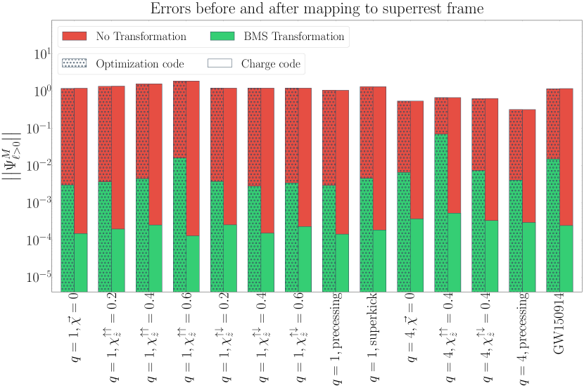
Figure 2: Comparison of the new charge-based frame fixing method (plain bars) to the previous method, which determined the BMS transformations by minimizing the $L^{2}$ norm of the $\ell>0$ components of the Moreschi supermomentum (patterned bars) when mapping to the superrest frame. The top of each bar is the norm of the $\ell>0$ components of the Moreschi supermomentum computed using Eq. (32). The red bars correspond to the norm when no frame fixing is performed, while the green bars correspond to the norm when the BMS frame is fixed. These simulations correspond to those found in Table 1.

For fixing the Poincaré freedom of our systems, Sec. II.1 pointed out that the ideal charge for fixing the translation and boost transformations is the center-of-mass charge, Eq. (17), and the ideal charge for fixing the rotation would typically be the usual angular momentum charge. However, because we want to map numerical waveforms to the PN BMS frame, for which the $\Psi_{1}$ and $\Psi_{2}$ Weyl scalars are unknown, for this mapping it is more convenient to use the charge that corresponds to the rotations on future null infinity, Eq. (19). Meanwhile, for mapping to superrest frame we use the spin vector, Eq. (21), because when we are in the center-of-mass frame of the remnant black hole there is no orbital angular momentum, so we need only care about the spin contribution. Apart from these Poincaré freedoms, Sec. II.2 illustrated that for the supertranslation freedom the Moreschi supermomentum can be used to map NR waveforms for comparison to either PN waveforms or QNM models. Thus, the entire BMS freedom of the system can be fixed via these charges: the center-of-mass charge, the rotation charge, and the Moreschi supermomentum.

For our NR systems, however, we find that obtaining BMS transformations from these charges must be done iteratively to ensure the convergence of the process. Consequently, we fix the BMS frame as follows:

1. Find the space translation and boost that minimize the center-of-mass charge $G^{a}$ over a large window; i.e., compute the center-of-mass charge and fit it with a linear function in time. The boost is the slope and the space translation is the intercept.

2. Find the proper supertranslation that maps the $\ell\geq 2$ components of $\Psi_{\text{M}}$ to the values obtained by PN (PN BMS frame) or to $M_{B}$ (superrest frame); i.e., compute the supertranslation using Eq. (35) where $\Psi_{\text{M}}^{\prime}$ is either $\Psi_{\text{M}}^{\text{PN}}$ or $M_{\text{B}}$. More practically, for fixing the frame using data at time $u=u_{0}$, we solve Eq. (35) for $\eth^{2}\bar{\eth}^{2}\alpha$ by taking $\alpha=u_{0}$ on the right-hand side, compute an approximate $\alpha$ by inverting $\eth^{2}\bar{\eth}^{2}$, and then iterate this procedure by taking $\alpha$ on the right-hand side to be the $\alpha$ obtained from the prior iteration until $\alpha$ converges.

3. Apply the supertranslation (the space translation and the proper supertranslation) to the original asymptotic quantities.

4. Compute the rotation that maps the rotation charge (either the charge in Eq. (19) for the PN BMS frame or in Eq. (21) for the superrest frame) to the values computed using a PN waveform (PN BMS frame) or to be parallel to the $+\hat{z}$-axis (superrest frame). We do this calculation using Davenport’s solution to Wahba’s problem to find the quaternion that best aligns the two charge vectors (see Sec. 5.3 of [67]).

5. Apply both the supertranslation and rotation to the original asymptotic quantities.

6. Repeat step I to obtain a new space translation and boost transformation for the transformed quantities.

7. Apply the center-of-mass transformation to the transformed asymptotic quantities.

8. If mapping to the PN BMS frame, perform a time/phase alignment using a 2D minimization of the error between the NR and PN strain waveforms.

When finding these BMS transformations from the BMS charges, we find them iteratively. Put differently, we solve for the transformation, transform the charge, solve for the transformation again, etc., until the transformation we are computing converges. This typically happens within five iterations, which matches the results of [9] for the center-of-mass transformations. Note that the reason why we apply a space translation and boost after solving for the supertranslation and rotation and transforming the asymptotic quantities is because we find that doing so is necessary to obtain the behavior that we expect from the center-of-mass transformation. Empirically we found that to minimize the new center-of-mass-charge, we must apply a space translation and boost after solving for the supertranslation and rotation, and transforming the asymptotic quantities.

As for the values of the transformations output by this charge-based frame fixing method, we find the following. The center-of-mass transformation is consistent with the work of [9]. The rotation quaternion tends to be close to the unit quaternion, except when working with systems that are precessing, in which case it is hard to predict. The modes of the supertranslation tend to be nearly zero when $m\not=0$ and fairly nontrivial when $m=0$. But this is simply because the $m=0$ memory modes dominate in PN theory, so we must correspondingly apply a supertranslation with larger $m=0$ coefficients.

All of the code used to perform these computations and frame transformations has been incorporated into the open-source code scri [19, 20, 21, 8], which has been validated by unit tests and prior works [19, 20, 21, 8, 9].

IV.2 Comparison of charge to optimizer method

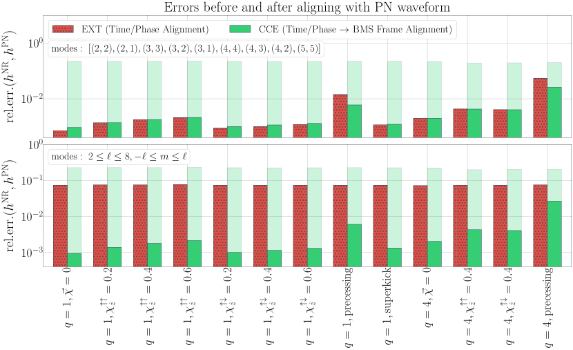
Figure 3: Comparison of the relative error between a CCE waveform and a PN waveform (green) to the relative error between an extrapolated waveform and a PN waveform (red). The relative error is computed over a three-orbit window that begins at $1200M$ past the initial time of the simulation. For the CCE waveforms, we show two errors: one where the error is computed when the time and phase freedom is fixed (faint) and one where the error is computed when the BMS freedom is fixed (full). With the extrapolated waveforms, we only fix the time and phase freedom. The top panel shows the relative error when only the $(2,2)$, $(2,1)$, $(3,3)$, $(3,2)$, $(3,1)$, $(4,4)$, $(4,3)$, $(4,2)$, and $(5,5)$ modes are included, while the bottom panel shows the error when every mode up to $\ell=8$ is included. These simulations correspond to those found in Table 1.

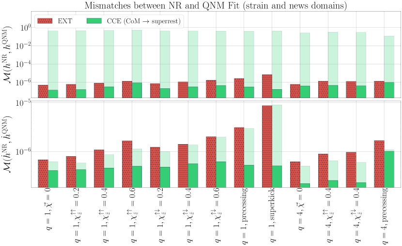
Figure 4: Comparison of the mismatch (the top of each bar) between a CCE waveform and the best-fit QNM model built from 100 modes chosen using the algorithm presented in [46] (green), to the mismatch obtained when using an extrapolated waveform instead of the CCE waveform (red). The mismatch is computed from the peak of the $L^{2}$ norm of the news onward to be consistent with [46]. The mass and spin of the remnant black hole are obtained from the Bondi rest mass and the spin charge, Eq. (21). For the CCE waveforms, we show two mismatches: one where the mismatch is computed using a CCE waveform in the center-of-mass frame of the remnant black hole (faint) and one where the CCE waveform is in the superrest frame of the remnant black hole (full). For the extrapolated waveforms, we only change each mode by a constant so that the waveform decays to zero at the end of the simulation. The top panel shows the mismatch between the strain waveforms, while the bottom panel shows the mismatch between the news waveforms. These simulations correspond to those found in Table 1.

Here we compare the charge-based scheme for fixing the BMS frame to the previous method, which relied on optimization algorithms. First, in Fig. 1 we show the relative error between the NR and PN strain waveforms once the NR system is mapped to the PN BMS frame. For reference, we show the relative error between these waveforms when no frame fixing is performed, or when only a time and phase fixing is performed by minimizing the absolute error between the NR and PN waveforms. Both methods compute the relative error between these two waveforms over a three-orbit window during the early inspiral phase and over the whole two-sphere for every spin-weighted spherical harmonic mode up to $\ell_{\text{max}}=8$. Explicitly,

$$\text{rel. err.}\left(h^{\text{NR}},h^{\text{PN}}\right)=||h^{\text{NR}}-h^{\text{PN}}||/||h^{\text{PN}}||,$$ (51)

where

$$||h||\equiv\sqrt{\int_{S^{2}}\left(\int_{u_{1}}^{u_{2}}\left|h(\ell_{\text{min}}\leq\ell\leq\ell_{\text{max}})\right|^{2}du\right)d\Omega}.$$ (52)

Here $u_{1}$ is the time that is $1200M$ past the beginning of the NR simulation, $u_{2}$ the time three-orbits beyond $u_{1}$, $\ell_{\text{min}}=2$, and $\ell_{\text{max}}=8$. As can be seen by comparing the plain green bars (charge-based method) to the patterned green bars (optimization algorithm) throughout Fig. 1, the charge-based frame fixing method produces an error that is nearly identical to the previous method for every BBH system, but with a typical run time of 30 minutes instead of 12 hours: a speedup of $\sim 24\times$.

In Fig. 2 we show the norm of the $\ell>0$ components of $\Psi_{\text{M}}$ during the final $100M$ of the numerical simulation, which is roughly $200M$ past the peak of the $L^{2}$ norm of the strain. We calculate this peak time by finding the time at which the square of Eq. (52), without the time integration, reaches its maximum value. As can be seen by comparing the plain green bars (charge-based method) to the patterned green bars (optimization algorithm), the new method produces errors that are roughly two orders of magnitude better than the optimization algorithm used in [9, 46]. Thus, it is evident that fixing the BMS frame to be the superrest frame of the remnant black hole is remarkably improved when using the new, charge-based frame fixing method. This improvement is primarily due to our ability to obtain more physically motivated supertranslations from the Moreschi supermomentum via Eq. (37), rather than an optimization algorithm that need not produce physical results.

IV.3 Comparison of NR to PN and QNMs

Thus far, we have shown why fixing the BMS frame of NR systems is important for comparing NR waveforms to PN waveforms or for modeling the ringdown phase of NR waveforms with QNMs. We now show why CCE waveforms and BMS frame fixing will help usher in the next generation of NR waveforms. We do so by comparing both CCE and extrapolated waveforms to PN waveforms in Fig. 3 and QNMs in Fig. 4.

In Fig. 3, like Fig. 1, we show the relative error between a NR and a PN strain waveform over a three-orbit window. In the top panel, we compute the relative error between these waveforms using the $(2,2)$, $(2,1)$, $(3,3)$, $(3,2)$, $(3,1)$, $(4,4)$, $(4,3)$, $(4,2)$, and $(5,5)$ modes. These are typically the most important modes without the $m=0$ modes. This collection of modes also matches those used in the NRHybSur3dq8 surrogate [68]. In the bottom panel, we instead compute the relative error using every mode up to $\ell=8$. The error obtained when using CCE waveforms is shown in green, while the error when using extrapolated waveforms is shown in red. Furthermore, for the CCE waveforms we show two errors: one where we perform a time/phase alignment (faint) and one where we perform a BMS frame alignment (full). For the extrapolated waveforms, however, the error is computed only with a time/phase alignment, since this is what has been used before Ref. [9]. As can be seen throughout the top panel, where the $m=0$ modes have been excluded, provided that we have fixed the BMS frame of the CCE waveforms, then these waveforms are on a par with the extrapolated waveforms. However, if we include the $m=0$ modes as in the bottom panel, then we find that the CCE waveforms are easily able to outperform the extrapolated waveforms for every type of system considered. This is because CCE waveforms, unlike extrapolated waveforms, contain memory effects that are also present in the PN treatment.

For working in the superrest frame, in Fig. 4, we show the mismatch between a NR waveform and a QNM model constructed from 100 QNM modes that are chosen using the ranking system presented in [46]. In the top panel we show the mismatch between the strain waveforms, while in the bottom panel we show the mismatch between the news waveforms, where the news waveform is just the time derivative of the strain waveform. The mismatch when using CCE waveforms is shown in green, while the mismatch when using extrapolated waveforms is shown in red. We compute the mismatch via

$$\mathcal{M}\left(h^{A},h^{B}\right)\equiv 1-\text{Re}\left[\frac{\langle h^{A},h^{B}\rangle}{\sqrt{\langle h^{A},h^{A}\rangle\langle h^{B},h^{B}\rangle}}\right],$$ (53)

where

$$\langle h^{A},h^{B}\rangle\equiv\int_{S^{2}}\int_{u_{0}}^{\infty}h^{A}\overline{h^{B}}\,du\,d\Omega.$$ (54)

Again, for CCE we show two mismatches: one where the CCE system is in the center-of-mass frame of the remnant black hole (faint) and one in the superrest frame of the remnant black hole (full). As can be seen in the top panel, mapping to the superrest frame is essential for modeling CCE waveforms with QNMs. This is because, unlike extrapolated waveforms, CCE waveforms contain memory effects so the CCE waveform will not decay to zero at timelike infinity, while the QNMs will. As a result, to model these NR waveforms with QNMs, fixing the supertranslation freedom is vitally important so that the waveforms do decay to zero. However, this is not the only impact that fixing the BMS frame has on NR waveforms. In the bottom panel, which shows the mismatch between the news waveforms, there continues to be an improvement by mapping to the superrest frame, even though there is no memory in these news waveforms. This is because when applying a supertranslation, there is also important mode mixing from expressing the first term of (13a) in terms of the untransformed time, i.e.,

$$\sigma(u^{\prime})=\sum\limits_{n=0}^{\infty}\frac{1}{n!}\left[\left(k(u-\alpha)-u\right)\frac{\partial}{\partial u}\right]^{n}\sigma(u).$$ (55)

For more on this, see Fig. 7 of [46] and the related text. Lastly, we should also note that by comparing Fig. 4 to Fig. 10 of [46], one can see that the mismatches obtained are practically identical, which means that the results of [46] should not be impacted by this new scheme for mapping to the superrest frame using BMS charges.

V Discussion

We have presented a new procedure for fixing the entire BMS frame of the data produced by NR simulations. The method relies on the use of BMS charges rather than optimization algorithms, like those used in [9, 46]. This charge-based frame fixing method fixes the system’s frame using the center-of-mass charge (Eq. (17)) and the rotation charge (Eq. (19)) for the Poincaré freedoms, and the Moreschi supermomentum $\Psi_{\text{M}}$ (Eq. (32)) for the supertranslation freedom. If the time and phase freedoms need to be fixed, e.g., for comparing NR systems to PN, then a 2D minimization of the error between NR and PN strain waveforms is performed. This code has been made publicly available in the python module scri [19, 20, 21, 8].

The BMS transformations are obtained by finding the transformation that changes the corresponding charge in a prescribed way. For example, to map to the system’s center-of-mass frame we find the transformation that maps the center-of-mass charge to have an average of zero. Accordingly, the transformations can be found much faster than if they were computed with a minimization scheme. For the BBH systems and frames we considered, we found that this new charge-based method converges in roughly $30$ minutes, rather than the $12$ or more hours that are needed by the previous optimization algorithm.

In particular, using the charge-based frame fixing, we mapped 14 binary systems to the PN BMS frame, i.e., the frame that PN waveforms are in. Apart from this, we mapped these systems to the superrest frame, i.e., the frame in which the metric of the remnant black hole matches the Kerr metric at timelike infinity. For mapping to the PN BMS frame, we fixed the Poincaré frame by mapping the center-of-mass charge to an average of zero and the rotation charge to match the rotation charge of the PN waveform. For the supertranslation freedom, however, we found that it was necessary to calculate the PN Moreschi supermomentum so that we could find the supertranslation via Eq. (35), which maps the numerical Moreschi supermomentum to the PN supermomentum during the early inspiral phase.

In Sec. III we performed this calculation by using the relation that writes $\Psi_{\text{M}}$ in terms of the energy flux (see, e.g., Eq. (II.2)). This calculation provides $\Psi_{\text{M}}$ to 3PN order without spins and 2PN order with spins. Moreover, this calculation also leads to oscillatory and spin-dependent memory terms that either have not been identified or have been missing from the existing PN strain expressions. These strain terms, as well as the complete expression for the PN Moreschi supermomentum, can be found in Appendices A and B.

In Sec. IV.1 we then described our procedure for fixing the BMS frame. In Sec. IV.2 we used our new code to map to the PN BMS frame (see Fig. 1) or to minimize the Moreschi supermomentum during ringdown, that is, map to the superrest frame (see Fig. 2). In each case, we compared with the previous code that relied on minimizers. Overall, we found that these two procedures tend to yield the same errors when mapping to the PN BMS frame, while the new charge-based procedure yields better errors when mapping to the superrest frame.

Finally, in Sec. IV.3 we considered CCE waveforms whose BMS frame has been fixed with this new method to be either the PN BMS frame or the superrest frame of the remnant black hole. We showed that such waveforms can notably outperform extrapolated waveforms, which are the current waveforms in the SXS catalog. This suggests that CCE waveforms and BMS frame fixing will be vital in the future for performing more correct numerical relativity simulations and conducting better waveform modeling.

Appendix A PN MORESCHI SUPERMOMENTUM

The complete results from our PN calculation of the modes of the Moreschi supermomentum are as follows:

$$\mathcal{P}^{(0,0)} =1+x\left(-\frac{3}{4}-\frac{\nu}{12}\right)+x^{2}\left(-\frac{27}{8}+\frac{19\nu}{8}-\frac{\nu^{2}}{24}\right)+x^{3}\left(-\frac{675}{64}+\left(\frac{34445}{576}-\frac{205\pi^{2}}{96}\right)\nu-\frac{155\nu^{2}}{96}-\frac{35\nu^{3}}{5184}\right),$$ (56a)

$$\mathcal{P}_{\text{spin}}^{(0,0)} =x^{3/2}\left(\frac{14S_{\ell}}{3M^{2}}+\frac{2\delta\Sigma_{\ell}}{M^{2}}\right)$$

$$\phantom{=.}+x^{2}\left(-\frac{16\vec{S}\cdot\vec{S}+3\vec{\Sigma}\cdot\vec{\Sigma}+32S_{\ell}^{2}+9\Sigma_{\ell}^{2}}{12M^{4}}-\frac{4\delta\left(\vec{S}\cdot\vec{\Sigma}+2S_{\ell}\Sigma_{\ell}\right)}{3M^{4}}+\frac{4\left(\vec{\Sigma}\cdot\vec{\Sigma}+2\Sigma_{\ell}^{2}\right)\nu}{3M^{4}}\right),$$ (56b)

$$\mathcal{P}^{(1,1)} =\frac{43}{70}\sqrt{\frac{3}{2}}\Bigg{\{}x^{3}\left(\frac{1856\delta\nu}{129}\right)\Bigg{\}},$$ (56c)

$$\mathcal{P}_{\text{spin}}^{(1,1)} =0,$$ (56d)

$$\mathcal{P}^{(2,1)} =0,$$ (56e)

$$\mathcal{P}_{\text{spin}}^{(2,1)} =\frac{61}{14\sqrt{30}}\Bigg{\{}x^{3/2}\left(-\frac{\left(S_{n}-iS_{\lambda}\right)}{M^{2}}-\frac{375\delta\left(\Sigma_{n}-i\Sigma_{\lambda}\right)}{488M^{2}}\right)$$

$$\phantom{=.\frac{61}{14\sqrt{30}}\Bigg{\{}}+x^{2}\Bigg{(}\frac{10\left(3S_{l}\left(S_{n}-iS_{\lambda}\right)+\Sigma_{l}\left(\Sigma_{n}-i\Sigma_{\lambda}\right)\right)}{61M^{4}}+\frac{15\delta\left(\left(S_{n}-iS_{\lambda}\right)\Sigma_{l}+S_{l}\left(\Sigma_{n}-i\Sigma_{\lambda}\right)\right)}{61M^{4}}$$

$$\phantom{=.\frac{61}{14\sqrt{30}}\Bigg{\{}+x^{2}\Bigg{(}}-\frac{30\nu\Sigma_{l}\left(\Sigma_{n}-i\Sigma_{\lambda}\right)}{61M^{4}}\Bigg{)}\Bigg{\}},$$ (56f)

$$\mathcal{P}^{(2,0)} =\frac{2}{7}\sqrt{5}\Bigg{\{}1+x\left(-\frac{4075}{4032}+\frac{67\nu}{48}\right)+x^{2}\left(-\frac{151877213}{67060224}-\frac{123815\nu}{44352}+\frac{205\nu^{2}}{352}\right)+\pi x^{5/2}\left(-\frac{253}{336}+\frac{253\nu}{84}\right)$$

$$\phantom{=.\frac{2}{7}\sqrt{5}\Bigg{\{}}+x^{3}\left(-\frac{4397711103307}{532580106240}+\left(\frac{700464542023}{13948526592}-\frac{205\pi^{2}}{96}\right)\nu+\frac{69527951\nu^{2}}{166053888}+\frac{1321981\nu^{3}}{5930496}\right)\Bigg{\}},$$ (56g)

$$\mathcal{P}_{\text{spin}}^{(2,0)} =\frac{2}{7}\sqrt{5}\Bigg{\{}x^{3/2}\left(\frac{16S_{\ell}}{3M^{2}}+\frac{419\delta\Sigma_{\ell}}{160M^{2}}\right)$$

$$\phantom{=.\frac{2}{7}\sqrt{5}\Bigg{\{}}+x^{2}\left(-\frac{128\vec{S}\cdot\vec{S}+24\vec{\Sigma}\cdot\vec{\Sigma}+256S_{\ell}^{2}+75\Sigma_{\ell}^{2}}{96M^{4}}-\frac{4\delta\left(\vec{S}\cdot\vec{\Sigma}+2S_{\ell}\Sigma_{\ell}\right)}{3M^{4}}+\frac{4\left(\vec{\Sigma}\cdot\vec{\Sigma}+2\Sigma_{\ell}^{2}\right)\nu}{3M^{4}}\right)\Bigg{\}},$$ (56h)

$$\mathcal{P}^{(3,3)} =-\frac{44x^{3}\delta\nu}{27\sqrt{35}},$$ (56i)

$$\mathcal{P}_{\text{spin}}^{(3,3)} =0,$$ (56j)

$$\mathcal{P}^{(3,1)} =\frac{223}{120\sqrt{21}}\Bigg{\{}x^{3}\left(\frac{3872\delta\nu}{223}\right)\Bigg{\}},$$ (56k)

$$\mathcal{P}_{\text{spin}}^{(3,1)} =0,$$ (56l)

$$\mathcal{P}^{(4,4)} =-\frac{4}{3}i\sqrt{\frac{2}{35}}x^{5/2}\nu,$$ (56m)

$$\mathcal{P}_{\text{spin}}^{(4,4)} =0,$$ (56n)

$$\mathcal{P}^{(4,1)} =0,$$ (56o)

$$\mathcal{P}_{\text{spin}}^{(4,1)} =\frac{13}{56\sqrt{5}}\Bigg{\{}x^{3/2}\left(-\frac{\left(S_{n}-iS_{\lambda}\right)}{M^{2}}-\frac{34\delta\left(\Sigma_{n}-i\Sigma_{\lambda}\right)}{39M^{2}}\right)$$

$$\phantom{=.\frac{13}{56\sqrt{5}}\Bigg{\{}}+x^{2}\Bigg{(}\frac{10\left(3S_{l}\left(S_{n}-iS_{\lambda}\right)+\Sigma_{l}\left(\Sigma_{n}-i\Sigma_{\lambda}\right)\right)}{117M^{4}}+\frac{5\delta\left(\left(S_{n}-iS_{\lambda}\right)\Sigma_{l}+S_{l}\left(\Sigma_{n}-i\Sigma_{\lambda}\right)\right)}{39M^{4}}$$

$$\phantom{=.\frac{13}{56\sqrt{5}}\Bigg{\{}+x^{2}\Bigg{(}}-\frac{10\nu\Sigma_{l}\left(\Sigma_{n}-i\Sigma_{\lambda}\right)}{39M^{4}}\Bigg{)}\Bigg{\}},$$ (56p)

$$\mathcal{P}^{(4,0)} =\frac{1}{42}\Bigg{\{}1+x\left(-\frac{180101}{29568}+\frac{27227\nu}{1056}\right)$$

$$\phantom{=.\frac{1}{42}\Bigg{\{}}+x^{2}\left(\frac{2201411267}{158505984}-\frac{34829479\nu}{432432}+\frac{844951\nu^{2}}{27456}\right)+x^{5/2}\left(-\frac{13565\pi}{1232}+\frac{13565\pi\nu}{308}\right)$$

$$\phantom{=.\frac{1}{42}\Bigg{\{}}+x^{3}\left(\frac{15240463356751}{781117489152}+\left(-\frac{1029744557245}{27897053184}-\frac{205\pi^{2}}{96}\right)\nu-\frac{4174614175\nu^{2}}{36900864}+\frac{221405645\nu^{3}}{11860992}\right)\Bigg{\}},$$ (56q)

$$\mathcal{P}_{\text{spin}}^{(4,0)} =\frac{1}{42}\Bigg{\{}x^{3/2}\left(\frac{10S_{\ell}}{M^{2}}+\frac{57\delta\Sigma_{\ell}}{8M^{2}}\right)$$

$$\phantom{=.\frac{1}{42}\Bigg{\{}}+x^{2}\left(-\frac{64\vec{S}\cdot\vec{S}+12\vec{\Sigma}\cdot\vec{\Sigma}+128S_{\ell}^{2}+41\Sigma_{\ell}^{2}}{48M^{4}}-\frac{4\delta\left(\vec{S}\cdot\vec{\Sigma}+2S_{\ell}\Sigma_{\ell}\right)}{3M^{4}}+\frac{4\left(\vec{\Sigma}\cdot\vec{\Sigma}+2\Sigma_{\ell}^{2}\right)\nu}{3M^{4}}\right)\Bigg{\}},$$ (56r)

$$\mathcal{P}^{(5,5)} =-\frac{36x^{3}\delta\nu}{5\sqrt{77}},$$ (56s)

$$\mathcal{P}_{\text{spin}}^{(5,5)} =0,$$ (56t)

$$\mathcal{P}^{(5,3)} =\frac{4x^{3}\delta\nu}{27\sqrt{385}},$$ (56u)

$$\mathcal{P}_{\text{spin}}^{(5,3)} =0,$$ (56v)

$$\mathcal{P}^{(5,1)} =\frac{2}{21}\sqrt{\frac{2}{165}}\Bigg{\{}x^{3}\left(26\delta\nu\right)\Bigg{\}},$$ (56w)

$$\mathcal{P}_{\text{spin}}^{(5,1)} =0,$$ (56x)

$$\mathcal{P}^{(6,0)} =-\frac{4195}{177408\sqrt{13}}x\Bigg{\{}1-\frac{3612\nu}{839}+x\left(-\frac{45661561}{6342840}+\frac{101414\nu}{2517}-\frac{48118\nu^{2}}{839}\right)+x^{3/2}\left(\frac{1248\pi}{839}-\frac{4992\pi\nu}{839}\right)$$

$$\phantom{=.-\frac{4195}{177408\sqrt{13}}x\Bigg{\{}}+x^{2}\left(\frac{3012132889099}{144921208320}-\frac{27653500031\nu}{191694720}+\frac{1317967427\nu^{2}}{4107744}-\frac{24793657\nu^{3}}{342312}\right)\Bigg{\}},$$ (56y)

$$\mathcal{P}_{\text{spin}}^{(6,0)} =0,$$ (56z)

$$\mathcal{P}^{(8,0)} =\frac{75601}{8895744\sqrt{17}}x^{2}\Bigg{\{}1-\frac{452070\nu}{75601}+\frac{733320\nu^{2}}{75601}$$

$$\phantom{=.\frac{75601}{8895744\sqrt{17}}x^{2}}+x\left(-\frac{265361599}{33869248}+\frac{18177898147\nu}{321757856}-\frac{722521125\nu^{2}}{5745676}+\frac{261283995\nu^{3}}{2872838}\right)\Bigg{\}},$$ (56aa)

$$\mathcal{P}_{\text{spin}}^{(8,0)} =0.$$ (56ab)

Appendix B PN STRAIN NEW MEMORY TERMS

The post-Minkowski expansion of gravitational waves in radiative coordinates yields the strain in terms of the radiative mass and current moments, $\mathrm{U}^{(\ell,m)}$ and $\mathrm{V}^{(\ell,m)}$ (see [48], but here following the conventions of [45]),

$$h^{(\ell,m)}=\frac{G}{\sqrt{2}Rc^{\ell+2}}\left(\mathrm{U}^{(\ell,m)}-\frac{i}{c}\mathrm{V}^{(\ell,m)}\right),$$ (57)

and when expressing the radiative moments in terms of the six types of source moments, $\mathrm{U}^{(\ell,m)}$ is then even further decomposed in terms that are called instantaneous, memory, tail, tail-of-tail, …pieces:

$$\mathrm{U}^{(\ell,m)}=\mathrm{U}^{(\ell,m)}_{\text{inst}}+\mathrm{U}^{(\ell,m)}_{\text{tail}}+\mathrm{U}^{(\ell,m)}_{\text{tail-tail}}+\mathrm{U}^{(\ell,m)}_{\text{mem}}+\ldots$$ (58)

Therefore, we simply define

$$h_{\text{mem}}^{(\ell,m)}=\frac{G}{\sqrt{2}Rc^{\ell+2}}\mathrm{U}^{(\ell,m)}_{\text{mem}}.$$ (59)

Then the memory arises as (Eq. (2.26) of [45], from Eq. (2.43c) of [70], and changing from STF tensors to spherical harmonics)

$$h_{\text{mem}}^{(\ell,m)} =\frac{16\pi G}{Rc^{4}}\sqrt{\frac{(\ell-2)!}{(\ell+2)!}}\times$$

$$\phantom{=.\frac{16\pi G}{Rc^{4}}}\int_{-\infty}^{u}du^{\prime}\int d\Omega\frac{dE^{\text{GW}}}{dud\Omega}\overline{Y}^{(\ell,m)},$$ (60)

where

$$\frac{dE^{\text{GW}}}{dud\Omega}=\frac{R^{2}}{16\pi G}|\dot{h}|^{2}.$$ (61)

Consequently, we find

$$h_{\text{mem}}^{(\ell,m)}=\frac{4}{Rc^{4}}\sqrt{\frac{(\ell-2)!}{(\ell+2)!}}\Psi^{(\ell,m)}_{\mathrm{M}},$$ (62)

or, in terms of the $\mathcal{P}^{(\ell,m)}$ decomposition of Eq. (46),

$$h_{\text{mem}}^{(\ell,m)}=\frac{2M\nu x}{R}\sqrt{\frac{(\ell-2)!}{(\ell+2)!}}\sqrt{4\pi}\mathcal{P}^{(\ell,m)}e^{-im\psi}.$$ (63)

Another way to derive this expression is by writing Eq. (II.2) with the strain, ignoring the contribution coming from the Bondi mass aspect, and then moving the factor of $\eth^{2}$ to the right-hand side.

Using Eq. (63) and the $\mathcal{P}^{(\ell,m)}$ expressions in Eq. (56) gives new oscillatory and spin-dependent memory terms which have not been identified or have been missing from the PN literature.

Finally we should point out the following interpretation of our BMS frame fixing procedure, by studying Eq. (62). Our procedure fixed the BMS frame by matching $\Psi_{\mathrm{M}}$, mode by mode, to $\Psi_{\mathrm{M}}^{\text{PN}}$. Then, because of the simple mode-wise proportionality $h_{\text{mem}}^{(\ell,m)}\propto\Psi_{\text{M}}^{(\ell,m)}$, it turns out that our frame-fixing is equivalent to matching $h_{\text{mem}}$ (except that, being a spin-weight $-2$ field, $h_{\text{mem}}$ is missing the $\ell=0,1$ information from $\Psi_{\text{M}}$).

References

- Abbott et al. [2021a] R. Abbott et al. (LIGO Scientific, Virgo), GWTC-2: Compact Binary Coalescences Observed by LIGO and Virgo During the First Half of the Third Observing Run, Phys. Rev. X 11, 021053 (2021a), arXiv:2010.14527 [gr-qc] .
- Abbott et al. [2021b] R. Abbott et al. (LIGO Scientific, VIRGO, KAGRA), GWTC-3: Compact Binary Coalescences Observed by LIGO and Virgo During the Second Part of the Third Observing Run, arXiv:2111.03606 [gr-qc] .
- Abbott et al. [2018] B. P. Abbott et al. (KAGRA, LIGO Scientific, Virgo, VIRGO), Prospects for observing and localizing gravitational-wave transients with Advanced LIGO, Advanced Virgo and KAGRA, Living Rev. Rel. 21, 3 (2018), arXiv:1304.0670 [gr-qc] .
- Berti et al. [2018a] E. Berti, K. Yagi, and N. Yunes, Extreme Gravity Tests with Gravitational Waves from Compact Binary Coalescences: (I) Inspiral-Merger, Gen. Rel. Grav. 50, 46 (2018a), arXiv:1801.03208 [gr-qc] .
- Berti et al. [2018b] E. Berti, K. Yagi, H. Yang, and N. Yunes, Extreme Gravity Tests with Gravitational Waves from Compact Binary Coalescences: (II) Ringdown, Gen. Rel. Grav. 50, 49 (2018b), arXiv:1801.03587 [gr-qc] .
- Bondi et al. [1962] H. Bondi, M. G. J. Van der Burg, and A. W. K. Metzner, Gravitational waves in general relativity, VII. Waves from axi-symmetric isolated system, Proceedings of the Royal Society of London. Series A. Mathematical and Physical Sciences 269, 21 (1962).
- Sachs and Bondi [1962] R. K. Sachs and H. Bondi, Gravitational waves in general relativity VIII. Waves in asymptotically flat space-time, Proceedings of the Royal Society of London. Series A. Mathematical and Physical Sciences 270, 103 (1962).
- Boyle [2016] M. Boyle, Transformations of asymptotic gravitational-wave data, Phys. Rev. D 93, 084031 (2016), arXiv:1509.00862 [gr-qc] .
- Mitman et al. [2021a] K. Mitman et al., Fixing the BMS frame of numerical relativity waveforms, Phys. Rev. D 104, 024051 (2021a), arXiv:2105.02300 [gr-qc] .
- Moreschi [1988] O. M. Moreschi, Supercenter of Mass System at Future Null Infinity, Class. Quant. Grav. 5, 423 (1988).
- Iozzo et al. [2021a] D. A. B. Iozzo et al., Comparing Remnant Properties from Horizon Data and Asymptotic Data in Numerical Relativity, Phys. Rev. D 103, 124029 (2021a), arXiv:2104.07052 [gr-qc] .
- Mitman et al. [2020] K. Mitman, J. Moxon, M. A. Scheel, S. A. Teukolsky, M. Boyle, N. Deppe, L. E. Kidder, and W. Throwe, Computation of displacement and spin gravitational memory in numerical relativity, Phys. Rev. D 102, 104007 (2020), arXiv:2007.11562 [gr-qc] .
- Mitman et al. [2021b] K. Mitman et al., Adding gravitational memory to waveform catalogs using BMS balance laws, Phys. Rev. D 103, 024031 (2021b), arXiv:2011.01309 [gr-qc] .
- Moxon et al. [2021] J. Moxon, M. A. Scheel, S. A. Teukolsky, N. Deppe, N. Fischer, F. Hébert, L. E. Kidder, and W. Throwe, The SpECTRE Cauchy-characteristic evolution system for rapid, precise waveform extraction, arXiv:2110.08635 [gr-qc] .
- Geroch et al. [1973] R. P. Geroch, A. Held, and R. Penrose, A space-time calculus based on pairs of null directions, J. Math. Phys. 14, 874 (1973).
- Boyle et al. [2019] M. Boyle et al., The SXS Collaboration catalog of binary black hole simulations, Class. Quant. Grav. 36, 195006 (2019), arXiv:1904.04831 [gr-qc] .
- Moreschi and Dain [1998] O. M. Moreschi and S. Dain, Rest frame system for asymptotically flat space-times, J. Math. Phys. 39, 6631 (1998), arXiv:gr-qc/0203075 .
- Dain and Moreschi [2000] S. Dain and O. M. Moreschi, General existence proof for rest frame systems in asymptotically flat space-time, Class. Quant. Grav. 17, 3663 (2000), arXiv:gr-qc/0203048 .
- Boyle et al. [2022] M. Boyle, D. Iozzo, L. Stein, A. Khairnar, H. Rüter, M. Scheel, V. Varma, and K. Mitman, moble/scri: v2022.8.0 (2022).
- Boyle [2013] M. Boyle, Angular velocity of gravitational radiation from precessing binaries and the corotating frame, Phys. Rev. D 87, 104006 (2013), arXiv:1302.2919 [gr-qc] .
- Boyle et al. [2014] M. Boyle, L. E. Kidder, S. Ossokine, and H. P. Pfeiffer, Gravitational-wave modes from precessing black-hole binaries, arXiv:1409.4431 [gr-qc] .
- Moreschi [1986] O. M. Moreschi, On angular momentum at future null infinity, Classical and Quantum Gravity 3, 503 (1986).
- Barnich and Troessaert [2010a] G. Barnich and C. Troessaert, Symmetries of asymptotically flat 4 dimensional spacetimes at null infinity revisited, Phys. Rev. Lett. 105, 111103 (2010a), arXiv:0909.2617 [gr-qc] .
- Strominger [2014] A. Strominger, On BMS Invariance of Gravitational Scattering, JHEP 07, 152, arXiv:1312.2229 [hep-th] .
- He et al. [2015] T. He, V. Lysov, P. Mitra, and A. Strominger, BMS supertranslations and Weinberg’s soft graviton theorem, JHEP 05, 151, arXiv:1401.7026 [hep-th] .
- Kapec et al. [2014] D. Kapec, V. Lysov, S. Pasterski, and A. Strominger, Semiclassical Virasoro symmetry of the quantum gravity -matrix, JHEP 08, 058, arXiv:1406.3312 [hep-th] .
- Pasterski et al. [2016] S. Pasterski, A. Strominger, and A. Zhiboedov, New Gravitational Memories, JHEP 12, 053, arXiv:1502.06120 [hep-th] .
- Barnich and Troessaert [2010b] G. Barnich and C. Troessaert, Aspects of the BMS/CFT correspondence, JHEP 05, 062, arXiv:1001.1541 [hep-th] .
- Strominger and Zhiboedov [2016] A. Strominger and A. Zhiboedov, Gravitational Memory, BMS Supertranslations and Soft Theorems, JHEP 01, 086, arXiv:1411.5745 [hep-th] .
- Flanagan and Nichols [2017] E. E. Flanagan and D. A. Nichols, Conserved charges of the extended Bondi-Metzner-Sachs algebra, Phys. Rev. D 95, 044002 (2017), arXiv:1510.03386 [hep-th] .
- de Andrade et al. [2001] V. C. de Andrade, L. Blanchet, and G. Faye, Third post-Newtonian dynamics of compact binaries: Noetherian conserved quantities and equivalence between the harmonic coordinate and ADM Hamiltonian formalisms, Class. Quant. Grav. 18, 753 (2001), arXiv:gr-qc/0011063 .
- Blanchet and Faye [2019] L. Blanchet and G. Faye, Flux-balance equations for linear momentum and center-of-mass position of self-gravitating post-Newtonian systems, Class. Quant. Grav. 36, 085003 (2019), arXiv:1811.08966 [gr-qc] .
- Compère et al. [2020] G. Compère, R. Oliveri, and A. Seraj, The Poincaré and BMS flux-balance laws with application to binary systems, JHEP 10, 116, arXiv:1912.03164 [gr-qc] .
- O’Shaughnessy et al. [2011] R. O’Shaughnessy, B. Vaishnav, J. Healy, Z. Meeks, and D. Shoemaker, Efficient asymptotic frame selection for binary black hole spacetimes using asymptotic radiation, Phys. Rev. D 84, 124002 (2011), arXiv:1109.5224 [gr-qc] .
- Dray and Streubel [1984] T. Dray and M. Streubel, Angular momentum at null infinity, Class. Quant. Grav. 1, 15 (1984).
- Wald and Zoupas [2000] R. M. Wald and A. Zoupas, A General definition of ’conserved quantities’ in general relativity and other theories of gravity, Phys. Rev. D 61, 084027 (2000), arXiv:gr-qc/9911095 .
- Zel’dovich and Polnarev [1974] Y. B. Zel’dovich and A. G. Polnarev, Radiation of gravitational waves by a cluster of superdense stars, Sov. Astron. 18, 17 (1974).
- Christodoulou [1991] D. Christodoulou, Nonlinear nature of gravitation and gravitational-wave experiments, Phys. Rev. Lett. 67, 1486 (1991).
- Thorne [1992] K. S. Thorne, Gravitational-wave bursts with memory: The christodoulou effect, Phys. Rev. D 45, 520 (1992).
- Flanagan and Nichols [2015] E. E. Flanagan and D. A. Nichols, Observer dependence of angular momentum in general relativity and its relationship to the gravitational-wave memory effect, Phys. Rev. D 92, 084057 (2015), [Erratum: Phys.Rev.D 93, 049905 (2016)], arXiv:1411.4599 [gr-qc] .
- Grant and Nichols [2022] A. M. Grant and D. A. Nichols, Persistent gravitational wave observables: Curve deviation in asymptotically flat spacetimes, Phys. Rev. D 105, 024056 (2022), arXiv:2109.03832 [gr-qc] .
- Seraj and Neogi [2022] A. Seraj and T. Neogi, Memory effects from holonomies, arXiv:2206.14110 [hep-th] .
- Ashtekar et al. [2020] A. Ashtekar, T. De Lorenzo, and N. Khera, Compact binary coalescences: Constraints on waveforms, Gen. Rel. Grav. 52, 107 (2020), arXiv:1906.00913 [gr-qc] .
- Arnowitt et al. [1959] R. Arnowitt, S. Deser, and C. W. Misner, Dynamical structure and definition of energy in general relativity, Phys. Rev. 116, 1322 (1959).
- Favata [2009] M. Favata, Post-Newtonian corrections to the gravitational-wave memory for quasi-circular, inspiralling compact binaries, Phys. Rev. D 80, 024002 (2009), arXiv:0812.0069 [gr-qc] .
- Magaña Zertuche et al. [2022] L. Magaña Zertuche, K. Mitman, N. Khera, L. C. Stein, M. Boyle, N. Deppe, F. Hébert, D. A. B. Iozzo, L. E. Kidder, J. Moxon, H. P. Pfeiffer, M. A. Scheel, S. A. Teukolsky, W. Throwe, and N. Vu, High precision ringdown modeling: Multimode fits and BMS frames, Phys. Rev. D 105, 104015 (2022).
- Compère and Long [2016] G. Compère and J. Long, Classical static final state of collapse with supertranslation memory, Class. Quant. Grav. 33, 195001 (2016), arXiv:1602.05197 [gr-qc] .
- Blanchet [2014] L. Blanchet, Gravitational Radiation from Post-Newtonian Sources and Inspiralling Compact Binaries, Living Rev. Rel. 17, 2 (2014), arXiv:1310.1528 [gr-qc] .
- Buonanno et al. [2013] A. Buonanno, G. Faye, and T. Hinderer, Spin effects on gravitational waves from inspiraling compact binaries at second post-Newtonian order, Phys. Rev. D 87, 044009 (2013), arXiv:1209.6349 [gr-qc] .
- Bohé et al. [2015] A. Bohé, G. Faye, S. Marsat, and E. K. Porter, Quadratic-in-spin effects in the orbital dynamics and gravitational-wave energy flux of compact binaries at the 3PN order, Class. Quant. Grav. 32, 195010 (2015), arXiv:1501.01529 [gr-qc] .
- Marsat [2015] S. Marsat, Cubic order spin effects in the dynamics and gravitational wave energy flux of compact object binaries, Class. Quant. Grav. 32, 085008 (2015), arXiv:1411.4118 [gr-qc] .
- Campbell and Morgan [1971] W. B. Campbell and T. Morgan, Debye Potentials for the Gravitational Field, Physica 53, 264 (1971).
- Bender et al. [1999] C. Bender, S. Orszag, and S. Orszag, Advanced Mathematical Methods for Scientists and Engineers I: Asymptotic Methods and Perturbation Theory, Advanced Mathematical Methods for Scientists and Engineers (Springer, 1999).
- [54] SXS Ext-CCE Waveform Database, https://data.black-holes.org/waveforms/extcce_catalog.html.
- [55] SXS Gravitational Waveform Database, http://www.black-holes.org/waveforms.
- Isoyama and Nakano [2018] S. Isoyama and H. Nakano, Post-Newtonian templates for binary black-hole inspirals: the effect of the horizon fluxes and the secular change in the black-hole masses and spins, Class. Quant. Grav. 35, 024001 (2018), arXiv:1705.03869 [gr-qc] .
- Pollney and Reisswig [2011] D. Pollney and C. Reisswig, Gravitational memory in binary black hole mergers, Astrophys. J. Lett. 732, L13 (2011), arXiv:1004.4209 [gr-qc] .
- Blanchet et al. [2004] L. Blanchet, T. Damour, G. Esposito-Farese, and B. R. Iyer, Gravitational radiation from inspiralling compact binaries completed at the third post-Newtonian order, Phys. Rev. Lett. 93, 091101 (2004), arXiv:gr-qc/0406012 .
- [59] https://www.black-holes.org/code/SpEC.html.
- Iozzo et al. [2021b] D. A. B. Iozzo, M. Boyle, N. Deppe, J. Moxon, M. A. Scheel, L. E. Kidder, H. P. Pfeiffer, and S. A. Teukolsky, Extending gravitational wave extraction using Weyl characteristic fields, Phys. Rev. D 103, 024039 (2021b), arXiv:2010.15200 [gr-qc] .
- Moxon et al. [2020] J. Moxon, M. A. Scheel, and S. A. Teukolsky, Improved Cauchy-characteristic evolution system for high-precision numerical relativity waveforms, Phys. Rev. D 102, 044052 (2020), arXiv:2007.01339 [gr-qc] .
- Deppe et al. [2020] N. Deppe, W. Throwe, L. E. Kidder, N. L. Fischer, C. Armaza, G. S. Bonilla, F. Hébert, P. Kumar, G. Lovelace, J. Moxon, E. O’Shea, H. P. Pfeiffer, M. A. Scheel, S. A. Teukolsky, I. Anantpurkar, M. Boyle, F. Foucart, M. Giesler, D. A. B. Iozzo, I. Legred, D. Li, A. Macedo, D. Melchor, M. Morales, T. Ramirez, H. R. Rüter, J. Sanchez, S. Thomas, and T. Wlodarczyk, SpECTRE (2020).
- Sarbach and Tiglio [2001] O. Sarbach and M. Tiglio, Gauge invariant perturbations of Schwarzschild black holes in horizon penetrating coordinates, Phys. Rev. D 64, 084016 (2001), arXiv:gr-qc/0104061 .
- Regge and Wheeler [1957] T. Regge and J. A. Wheeler, Stability of a Schwarzschild singularity, Phys. Rev. 108, 1063 (1957).
- Zerilli [1970] F. J. Zerilli, Effective potential for even parity Regge-Wheeler gravitational perturbation equations, Phys. Rev. Lett. 24, 737 (1970).
- Boyle and Mroue [2009] M. Boyle and A. H. Mroue, Extrapolating gravitational-wave data from numerical simulations, Phys. Rev. D 80, 124045 (2009), arXiv:0905.3177 [gr-qc] .
- Markley and Crassidis [2014] F. L. Markley and J. L. Crassidis, Fundamentals of Spacecraft Attitude Determination and Control (Springer New York, 2014).
- Varma et al. [2019] V. Varma, S. E. Field, M. A. Scheel, J. Blackman, L. E. Kidder, and H. P. Pfeiffer, Surrogate model of hybridized numerical relativity binary black hole waveforms, Phys. Rev. D 99, 064045 (2019), arXiv:1812.07865 [gr-qc] .
- Bernard et al. [2018] L. Bernard, L. Blanchet, G. Faye, and T. Marchand, Center-of-Mass Equations of Motion and Conserved Integrals of Compact Binary Systems at the Fourth Post-Newtonian Order, Phys. Rev. D 97, 044037 (2018), arXiv:1711.00283 [gr-qc] .
- Blanchet and Damour [1992] L. Blanchet and T. Damour, Hereditary effects in gravitational radiation, Phys. Rev. D 46, 4304 (1992).