An Effective Field Theory for Large Oscillons

Abstract

We consider oscillons — localized, quasiperiodic, and extremely long-living classical solutions in models with real scalar fields. We develop their effective description in the limit of large size at finite field strength. Namely, we note that nonlinear long-range field configurations can be described by an effective complex field $\psi(t,\boldsymbol{x})$ which is related to the original fields by a canonical transformation. The action for $\psi$ has the form of a systematic gradient expansion. At every order of the expansion, such an effective theory has a global U(1) symmetry and hence a family of stationary nontopological solitons — oscillons. The decay of the latter objects is a nonperturbative process from the viewpoint of the effective theory. Our approach gives an intuitive understanding of oscillons in full nonlinearity and explains their longevity. Importantly, it also provides reliable selection criteria for models with long-lived oscillons. This technique is more precise in the nonrelativistic limit, in the notable cases of nonlinear, extremely long-lived, and large objects, and also in lower spatial dimensions. We test the effective theory by performing explicit numerical simulations of a $(d+1)$-dimensional scalar field with a plateau potential.

1 Introduction

Oscillons Gleiser:1993pt are compact, almost periodic, and long-lived classical solutions in models with real bosonic fields, notably, the scalar field $\varphi(t,\,\boldsymbol{x})$. These objects were discovered in explicit numerical simulations in the 70s Kudryavtsev:1975dj ; Bogolyubsky:1976nx , but even now theoretical reasons for their widespread existence and extreme longevity are poorly understood. To date, the oscillons were found in a plethora of theories with attractive self-interactions Kolb:1993zz ; Piette:1997hf ; Gleiser:2008dt ; Amin:2010jq ; Gleiser:2010qt ; Salmi:2012ta ; Amin:2013ika ; Sakstein:2018pfd ; Olle:2019kbo ; Zhang:2021xxa . All of them radiate waves and eventually disappear, but before that live for $10^{3}$ oscillation cycles in generic models Zhang:2020bec and up to $10^{14}$ cycles in special cases Olle:2020qqy . Such large numbers are highly remarkable and deserve to be explained, as the models with oscillons usually lack large, small, or fine-tuned parameters.

Meanwhile, the oscillons are becoming a workhorse in cosmology. They nucleate excessively during generation of axion Kolb:1993hw ; Vaquero:2018tib ; Buschmann:2019icd ; Gorghetto:2020qws or ultra-light OHare:2021zrq dark matter, may accompany cosmological phase transitions Gleiser:1993pt ; Copeland:1995fq ; Dymnikova:2000dy ; Farhi:2007wj ; Gleiser:2010qt ; Bond:2015zfa and be formed by the oscillating inflaton field during preheating Amin:2010dc ; Amin:2011hj ; Hong:2017ooe ; Sang:2020kpd . Their close relatives — gravitationally bound boson stars — appear in the centers of the smallest axion Levkov:2018kau ; Eggemeier:2019jsu ; Chen:2020cef ; Chan:2022bkz and fuzzy Schive:2014dra ; Schive:2014hza ; Veltmaat:2018dfz dark matter structures. Cosmological oscillons may produce gravitational waves Zhou:2013tsa ; Liu:2017hua ; Lozanov:2019ylm ; Sang:2019ndv , participate in baryogenesis Lozanov:2014zfa , conceive axion miniclusters Kolb:1993hw ; Vaquero:2018tib ; Xiao:2021nkb , or create a population of primordial black holes Cotner:2019ykd ; Kou:2019bbc , cf. Garani:2021gvc . With sufficiently large lifetimes, they may even act as dark matter candidates Olle:2020qqy . All of this requires more systematic studies of these fascinating objects.

Presently, the only model-independent method to describe oscillons is based on nonrelativistic (small-amplitude) expansion Dashen:1975hd ; Kosevich1975 ; Fodor:2008es ; Fodor:2019ftc . This technique applies to quasiperiodic field configurations with sufficiently large sizes $R$, weak fields $\varphi(t,\,\boldsymbol{x})$, and oscillation frequencies $\omega$ nearing the field mass $m$,

$$\mbox{small-amplitude:}\qquad R\gg m^{-1}\;,\qquad\omega\approx m\;,\qquad\varphi\;\mbox{ is small}\;.$$ (1)

In terms of particle physics, such configurations describe condensates of weakly interacting nonrelativistic bosons with small momenta $R^{-1}$ and low binding energies ${m-\omega\ll m}$. Since the particle number $N$ is conserved in the nonrelativistic limit, it is natural to expect that the bosons form stable localized lumps — oscillons — if their self-interactions are attractive. Solving the classical field equations order-by-order in the field amplitude, one can compute the profiles and energies of oscillons Dashen:1975hd ; Kosevich1975 ; Fodor:2008es . Besides, exponentially small effects complementary to the nonrelativistic expansion describe radiation from these objects and estimate their lifetimes Segur:1987mg ; Fodor:2008du ; Fodor:2009kf ; Fodor:2019ftc .

The above technique is unsatisfactory in three respects. First, it fails to describe exceptionally long-lived, large-amplitude, and large-size oscillons Olle:2019kbo ; Zhang:2020bec ; Olle:2020qqy discovered in scalar models with almost quadratic monodromy potentials Silverstein:2008sg ; McAllister:2008hb . In some other cases, the nonrelativistic expansion requires a modification Amin:2010jq . To explain stability of large-amplitude oscillons, Refs. Kasuya:2002zs ; Kawasaki:2015vga suggested existence of an adiabatic invariant that is approximately conserved during evolution of nonlinear oscillating fields. This quantity generalizes the particle number $N$. Then the oscillons minimize the energy at a given value of the invariant, similarly to Q-balls Friedberg:1976me ; Coleman:1985ki ; Nugaev:2019vru . However, a consistent off-shell and strong-field definition of the adiabatic invariant is absent so far.

Second, the above nonrelativistic expansion is asymptotic. In some models, it poorly approximates oscillon profiles even if the value of the nonrelativistic parameter is small Fodor:2008es . Third, generic three-dimensional oscillons with $\omega\approx m$ are, in fact, unstable Zakharov12 . In this case the lowest term of the small-amplitude expansion gives qualitatively incorrect predictions for oscillons with lower $\omega$.

In this paper we develop an Effective Field Theory (EFT) description of oscillons with large size and any amplitude,

$$\mbox{EFT:}\qquad R\gg m^{-1}\;,\qquad\mbox{$\varphi$ is arbitrary.}$$ (2)

This regime is natural: crude estimates show Gleiser:2004an that long-living oscillating objects can exist only in low enough dimensions and with large enough sizes. For definiteness we will consider one real scalar field $\varphi$ with symmetric potential; generalization to other cases is straightforward.

We observe that as long as the spatial scales are large and the gradient terms in the equations are suppressed, the classical field $\varphi(t,\,\boldsymbol{x})$ at any $\boldsymbol{x}$ performs fast, almost mechanical oscillations in the scalar potential $V(\varphi)$. Then the proper slowly varying EFT variables are the amplitude $I(t,\,\boldsymbol{x})$ and phase $\theta(t,\,\boldsymbol{x})$ of the oscillations — the action and angle variables in the mechanical system with potential $V$. These quantities can be combined into one complex EFT field,

$$\psi(t,\,\boldsymbol{x})=\sqrt{I}\,\cdot\mathrm{e}^{-i\theta}\;.$$ (3)

From the viewpoint of the original theory, $\psi$ and $\psi^{*}$ are related to $\varphi$ and $\partial_{t}\varphi$ by a canonical transformation. We demonstrate that the effective classical action for their slowly-varying parts can be written in the form of a systematic gradient expansion, where the terms like $|\partial_{\boldsymbol{x}}\psi|^{2}$ and $|\partial_{\boldsymbol{x}}\psi|^{4}$ appear in the first and second orders, respectively. Most importantly, at any order the effective action is invariant under global U(1) symmetry $\psi\to\psi\,\mathrm{e}^{-i\alpha}$ and hence has a conserved charge

$$N=\int d^{d}\boldsymbol{x}\,|\psi|^{2}+\mbox{corrections}\;.$$ (4)

When evaluated in the leading order on the classical solution, this charge coincides with the adiabatic invariant of Refs. Kasuya:2002zs ; Kawasaki:2015vga . We conclude that our effective theory possesses a family of oscillons which are indeed the nontopological solitons minimizing the energy at a given $N$.

Notably, the same effective approach may be useful for studying some mechanical systems with many degrees of freedom, see Appendix B for details.

Our classical EFT is way simpler than direct computation of tree diagrams suggested in Braaten:2015eeu ; Braaten:2016kzc ; Visinelli:2017ooc and more powerful than their partial resummation in Eby:2014fya . It generalizes nonrelativistic EFT approaches of Mukaida:2016hwd ; Eby:2018ufi ; Salehian:2021khb which can be restored by re-expanding the effective action in field amplitudes. The latter re-expansion also reproduces all small-amplitude results Dashen:1975hd ; Kosevich1975 ; Fodor:2008es ; Fodor:2019ftc for oscillons.

But even more importantly, the effective theory can explain essentially nonlinear large-amplitude oscillons Amin:2010jq ; Olle:2019kbo ; Zhang:2020bec ; Olle:2020qqy and clarify conditions for their existence and longevity. Namely, these objects exist within the EFT if the scalar potential of the model satisfies certain requirements summarized in Sec. 4.1 and in Discussion. For linear stability, their charges $N(\omega)$ should satisfy the Vakhitov-Kolokolov criterion vk ; Zakharov12 ; Amin:2010jq ; Nugaev:2019vru . The decay of oscillons is expected to be a nonperturbative process from the viewpoint of the gradient expansion, similarly to the nonrelativistic case Segur:1987mg ; Fodor:2008du ; Fodor:2009kf ; Fodor:2019ftc . We do not consider such processes in this paper but note that oscillons should be exponentially long-lived whenever Eq. (2) holds and the EFT works. This leads to additional conditions on the potential, see Sec. 4.2 and Discussion.

We test the EFT by performing spherically symmetric simulations of a $(d+1)$-dimensional scalar field with the plateau potential which is typical for $\alpha\mbox{-attractor}$ inflation Kallosh:2013hoa and is frequently employed in oscillon studies Zhang:2020bec . We find that the EFT correctly describes oscillons: qualitatively in $d=3$ dimensions, precisely in $d=1$ and 2, and exactly in the nonrelativistic limit ${\omega\to m}$.

As a final result, we explain significant dependence of the oscillon stability properties on the dimensionality $d$ of space Gleiser:2004an . Note that full classical equation for the spherically-symmetric scalar field $\varphi(t,\,r)$ has a nontrivial formal limit $d\to 0$. We observe that in $d=0$ it has an ever-lasting and strictly periodic stationary solution — a “zero-dimensional oscillon.” This explains why oscillons mostly appear in low-dimensional models and become increasingly unstable Gleiser:2004an at larger $d$. Amusingly, our EFT also becomes exact in $d\to 0$, since all its higher-order terms are proportional to $d$. As a consequence, it works better in lower dimensions.

The paper is organized as follows. We start with an explicit numerical example of oscillon in Sec. 2. Then we introduce the leading-order EFT in Sec. 3 and illustrate it in a mechanical model in Appendix B. In Sec. 4, we study solitonic oscillons within the EFT and formulate the conditions for their existence and longevity. Section 5 tests effective theory against explicit numerical simulations. The formal limit of zero dimensions and higher-order corrections are considered in Secs. 6 and 7, respectively. For clarity, we calculate the corrections in the mechanical model of Appendix B as well. We perform comparison with small-amplitude expansion in Sec 8 and discuss future prospects in Sec. 9. Appendices A and C to E include details of numerical and analytical calculations.

2 Oscillons: numerical illustration

We consider real scalar field $\varphi(t,\,\boldsymbol{x})$ with nonlinear potential $V(\varphi)$ in $(d+1)$ dimensions. It satisfies the equation

$$(\partial_{t}^{2}-\Delta)\varphi=-V^{\prime}(\varphi)\;,$$ (5)

where $\Delta$ is a $d$-dimensional Laplacian and the prime denotes $\varphi$ derivative. Let us numerically demonstrate that the oscillons appear if $V(\varphi)$ is chosen appropriately.

For these purposes, we select $d=3$ dimensions, a potential motivated by $\alpha$-attractor inflation Kallosh:2013hoa ; Zhang:2020bec ,

$$V(\varphi)=\frac{1}{2}\tanh^{2}\varphi\;,$$ (6)

and adopt dimensionless units with field mass equal to one, $m=1$. Importantly, the potential (6) is attractive, i.e. grows slower than $\varphi^{2}$. This property is usually held responsible for formation of long-living lumps — oscillons.

Starting from the Gaussian initial data $\varphi=\varphi_{0}\exp(-r^{2}/\sigma^{2})$ and $\partial_{t}\varphi=0$ at ${t=0}$, we numerically solve equation for the spherically-symmetric field $\varphi(t,\,r)$, where $r\equiv|\boldsymbol{x}|$ is the radial coordinate. Details of this procedure are presented in Appendix A.

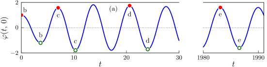
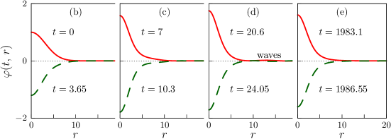
Figure 1: Numerical evolution of a spherically-symmetric scalar field $\varphi(t,\,r)$ with Gaussian initial data ($\varphi_{0}=1$ and $\sigma=20$) in the $(3+1)$-dimensional model (6). Figure (a) shows the field $\varphi(t,\,0)$ in the center ${r=0}$ as a function of time, while Figs. (b)—(e) display configurations at time moments of maximal (solid lines) and minimal (dashed lines) values of $\varphi(t,\,0)$. The latter are marked in Fig. (a) with filled and empty circles, respectively.

The result is demonstrated in Fig. 1 and in the movie movie . After a short period of aperiodic nonlinear wobbling (Figs. 1b,c and the left-hand side of Fig. 1a) the field lump in the center shakes off some outgoing waves (tiny, but seen in Fig. 1d) and settles in an almost periodic long-living configuration (Fig. 1e and the right-hand side of Fig. 1a). This is the oscillon to be studied in what follows.

We stress that oscillons are not specific to the model (6) or to the Gaussian initial data. They appear in the spectacular number of attractive theories in low enough $d$, see Refs. Kolb:1993zz ; Piette:1997hf ; Gleiser:2008dt ; Amin:2010jq ; Gleiser:2010qt ; Salmi:2012ta ; Amin:2013ika ; Sakstein:2018pfd ; Olle:2019kbo ; Zhang:2020bec ; Cyncynates:2021rtf ; Zhang:2021xxa . Although the model (6) is generic from the viewpoint of oscillon longevity, these objects typically survive to the end of our simulations lasting up to $10^{5}$ cycles. Such lifetimes deserve to be explained.

3 Classical EFT

Now, we construct classical effective field theory (EFT) for nonlinear oscillons in the limit of large size (2) or, more specifically, at

$$|\partial_{i}\varphi|\ll m\varphi\;,$$ (7)

where the field mass is restored and $\partial_{i}$ is the spatial derivative. Soon we will see that in generic models this condition gets parametrically satisfied only in the nonrelativistic limit Fodor:2008es when the oscillon frequency $\omega$ approaches $m$ and the field amplitude becomes small. But there are also special models Olle:2019kbo ; Zhang:2020bec ; Olle:2020qqy with exceptionally long-lived and large-amplitude oscillons, the sizes of which are proportional to large parameters. To cover both cases, we work at finite frequency $\omega$ and consider nonlinear fields.

Imagine that in the roughest approximation we can ignore the term with the spatial derivatives in the field equation (5). This leaves a nonlinear mechanical system ${\partial^{2}_{t}\varphi=-V^{\prime}(\varphi)}$ which can be solved in the action-angle variables LL1 ; Arnold . Namely, one introduces the momentum $\pi_{\varphi}=\partial_{t}\varphi=\sqrt{2h-2V(\varphi)}$, where $h$ is a mechanical energy, and then performs a canonical transformation to the new variables $I$ and $\theta$,

$$\varphi=\Phi(I,\theta)\;,\qquad\qquad\partial_{t}\varphi=\pi_{\varphi}=\Pi(I,\theta)\;,$$ (8)

in such a way that the action $I$ is conserved during the mechanical motion and the angle $\theta$ is canonically conjugate to it. More explicitly,

$$I(h)=\frac{1}{2\pi}\oint\pi_{\varphi}(h,\,\varphi)\,d\varphi\;,$$ (9)

where the integration is done over the oscillation period, and the angle equals

$$\theta(I,\,\varphi)=\frac{\partial}{\partial I}\;\int_{\varphi_{h}}^{\varphi}\pi_{\varphi}(h(I),\,\varphi^{\prime})\,d\varphi^{\prime}\;.$$ (10)

Hereafter, $h(I)$ is obtained by inverting Eq. (9) and $\theta=0$ corresponds to a turning point $\varphi=\varphi_{h}$ with $\pi_{\varphi}=0$. Recalling that ${h=\pi_{\varphi}^{2}/2+V(\varphi)}$, one can express $\varphi$ and $\pi_{\varphi}$ from Eqs. (9) and (10) obtaining $\Phi(I,\,\theta)$ and $\Pi(I,\,\theta)$. Note that the latter functions can be evaluated explicitly for some potentials, approximately in other cases, or efficiently represented in the form of convergent power series using computer algebra. Once this is done, the solution to the mechanical equation would be ${I=\mbox{const}}$ and $\theta=\Omega\,t+\mbox{const}$, where $\Omega(I)=dh/dI$ is the frequency of oscillations in the potential $V(\varphi)$. As designed, $I$ remains constant during the nonlinear oscillations and $\theta$ increases by $2\pi$ every period.

In field theory, the terms with the spatial derivatives cannot be ignored altogether even if they are suppressed, as they determine the spatial profile of the oscillon. Nevertheless, Eq. (8) still defines a canonical transformation from $\varphi$ and $\pi_{\varphi}=\partial_{t}\varphi$ to $I(t,\,\boldsymbol{x})$ and $\theta(t,\,\boldsymbol{x})$. The latter variables are not the true action and angle in field theory, but they still parameterize the amplitude and phase of local oscillations at every point. It is natural to expect that $I$ and $\partial_{t}\theta$ slowly depend on space and time in the limit of large size, unlike the fast-oscillating ${\varphi(t,\,\mathbf{x})}$. We will use them as smooth variables in the leading-order EFT.

Now, we evaluate classical effective action for slowly varying $I$ and $\theta$. We substitute the transformation (8) into the action of a scalar field,

$${\cal S}=\int dt\,d^{d}\boldsymbol{x}\left(\pi_{\varphi}\partial_{t}\varphi-h-\frac{1}{2}(\partial_{i}\varphi)^{2}\right)\;,\qquad h\equiv\pi_{\varphi}^{2}/2+V(\varphi)\;,$$ (11)

where the “mechanical Hamiltonian” $h(\varphi,\,\pi_{\varphi})$ is introduced for convenience. Since the transformation (8) is canonical, $\int dt\,\pi_{\varphi}\partial_{t}\varphi=\int dt\,I\partial_{t}\theta$. Besides, $h$ is a function of $I$ defined in Eq. (9). Finally, we note that the subdominant term with spatial derivatives ${f=(\partial_{i}\varphi)^{2}}$ is integrated in the action (11) over many oscillation periods. Thus, let us explicitly average it over period, i.e. over $\theta$ which changes almost linearly in time,

$$\langle f\rangle=\frac{1}{2\pi}\int_{0}^{2\pi}f(I,\theta)\,d\theta\;.$$ (12)

Using Eq. (8), we find,

$$\langle(\partial_{i}\varphi)^{2}\rangle\approx\frac{(\partial_{i}I)^{2}}{\mu_{I}(I)}+\frac{(\partial_{i}\theta)^{2}}{\mu_{\theta}(I)}\;,\qquad\qquad\frac{1}{\mu_{I}}\equiv\left\langle(\partial_{I}\Phi)^{2}\right\rangle\;,\qquad\frac{1}{\mu_{\theta}}\equiv\left\langle(\partial_{\theta}\Phi)^{2}\right\rangle\;,$$ (13)

where we moved all slowly varying quantities $\partial_{i}I$ and $\partial_{i}\theta$ out of the averages, introduced ${\partial_{I}\equiv\partial/\partial I}$ and $\partial_{\theta}\equiv\partial/\partial\theta$, and observed that the cross-term $\langle\partial_{I}\Phi\,\partial_{\theta}\Phi\rangle\partial_{i}I\partial_{i}\theta$ vanishes due to time reflection symmetry $t\to-t$, $\theta\to-\theta$. Indeed, recall that $\theta=0$ corresponds to a turning point $\pi_{\varphi}=0$. Then $\Phi$ is an even function of $\theta$ and $\partial_{I}\Phi\partial_{\theta}\Phi$ is odd with zero average.

Collecting the terms, we obtain the leading-order effective action,

$$\mathcal{S}_{\mathrm{eff}}=\int dt\,d^{d}{\boldsymbol{x}}\left(I\partial_{t}\theta-h(I)-\frac{(\partial_{i}I)^{2}}{2\mu_{I}(I)}-\frac{(\partial_{i}\theta)^{2}}{2\mu_{\theta}(I)}\right)\;,$$ (14)

where $\mu_{I}$ and $\mu_{\theta}$ are explicitly given by Eqs. (13) if the transformation $\Phi$ is known. The same action takes more familiar form in terms of a complex field $\psi(t,\,\boldsymbol{x})$ introduced in Eq. (3),

$$\mathcal{S}_{\mathrm{eff}}=\int dt\;d^{d}\boldsymbol{x}\left(i\psi^{*}\partial_{t}\psi-h(|\psi|^{2})-\frac{|\partial_{i}\psi|^{2}}{2\mu_{1}}-\frac{1}{2\mu_{2}}\left[\psi^{*2}(\partial_{i}\psi)^{2}+\mathrm{h.c.}\right]\right)\;,$$ (15)

where $\mu_{1}\equiv 2I\mu_{I}\mu_{\theta}/(4I^{2}\mu_{\theta}+\mu_{I})$ and $\mu_{2}\equiv 4I^{2}\mu_{I}\mu_{\theta}/(4I^{2}\mu_{\theta}-\mu_{I})$. We arrived at a nonlinear Schrödinger model for $\psi$ with the form factors $h$, $\mu_{1}$, and $\mu_{2}$ depending on $I\equiv|\psi|^{2}$. An equation for the evolution of long-range fields can be obtained by varying Eq. (14) over $I$ and $\theta$, or Eq. (15) over $\psi$ and $\psi^{*}$. In particular,

$$\partial_{t}I=\partial_{i}(\partial_{i}\theta/\mu_{\theta})\;,\qquad\qquad\partial_{t}\theta=\Omega-\frac{\Delta I}{\mu_{I}}+\frac{\partial_{I}\mu_{I}}{2\mu_{I}^{2}}\,(\partial_{i}I)^{2}-\frac{\partial_{I}\mu_{\theta}}{2\mu_{\theta}^{2}}\,(\partial_{i}\theta)^{2}\;,$$ (16)

with $\Omega\equiv\partial_{I}h$. An equivalent equation for $\psi$ has the form of a modified nonlinear Schrödinger equation.

It is worth stressing that the above effective approach is approximate due to period averaging in Eq. (13). We will see in Sec. 7 that corrections to the effective action are suppressed by at least four spatial derivatives of $I$ and $\theta$. This will confirm that the effective theory works for the long-range fields, indeed.

To support the classical EFT even further, we demonstrate in Appendix B that it correctly reproduces the spectrum of two weakly coupled mechanical oscillators. We expect that in the future this method may be helpful for studies of some nonlinear dynamical systems.

The most important property of the effective theory is a global U(1) symmetry

$$\theta\to\theta+\alpha\qquad\mbox{or}\qquad\psi\to\psi\,\mathrm{e}^{-i\alpha}\;,\quad\psi^{*}\to\psi^{*}\,\mathrm{e}^{i\alpha}\;,$$

which appears after averaging over $\theta$ in Eq. (13). As a consequence, the U(1) charge $N$ given by the first term in Eq. (4) conserves: $\partial_{t}N=0$ according to Eqs. (16). On-shell, the value of this charge coincides with the “adiabatic invariant” in Refs. Kasuya:2002zs ; Kawasaki:2015vga :

$$N=\frac{1}{2\pi}\int d^{d}\boldsymbol{x}\oint\pi_{\varphi}\,d\varphi=\frac{1}{2\pi}\int d^{d}\boldsymbol{x}\oint dt\,(\partial_{t}\varphi)^{2}$$ (17)

where all integrals cover for one oscillation period and we used Eq. (9). Note that Eq. (17) is convenient for finding the values of $N$ on quasiperiodic solutions, but unlike Eq. (4), it is useless off-shell. In the next Section we will observe that under certain conditions conservation of charge leads to appearance of stable nontopological solitons similar to $Q$-balls — the oscillons.

We finish this Section by illustrating the calculation of the leading-order effective action in the model (6). Equation (9) gives,

$$h(I)=I-I^{2}/2\;.$$ (18)

This means that the frequency of mechanical oscillations in the potential $V(\varphi)$ is ${\Omega=\partial_{I}h=1-I}$. The canonical transformation $\varphi=\Phi(I,\,\theta)$ and $\pi_{\varphi}=\Pi(I,\,\theta)$ is then obtained using Eq. (10) and the definition of $h(\varphi,\,\pi_{\varphi})$:

$$\Phi=\operatorname{arcsinh}\left(\frac{\sqrt{I(2-I)}}{1-I}\,\cos\theta\right),\qquad\Pi=-\frac{(1-I)\sin\theta}{\sqrt{[I(2-I)]^{-1}-\sin^{2}\theta}}\;.$$ (19)

One can readily check that the Poisson bracket of these functions equals one. Next, we evaluate the integrals (13) over $\theta$ and obtain the time-averaged form factors,

$$\mu_{I}=I(2-I)^{2}(1-I)^{2}\;,\qquad\qquad\mu_{\theta}=I^{-1}-1\;.$$ (20)

The coefficients in the action for $\psi$ immediately follow:

$$\mu_{1}=\frac{2(1-I)^{2}(2-I)^{2}}{4+(1-I)(2-I)^{2}}\;,\qquad\qquad\mu_{2}=\frac{4I(1-I)^{2}(2-I)^{2}}{4-(1-I)(2-I)^{2}}\;;$$ (21)

notably, $\mu_{1}$ and $\mu_{2}/I$ are finite in the weak-field limit $I\to 0$. We conclude that once the scalar potential is fixed, the EFT has an explicit form of a nonlinear Schrödinger-like model for $\psi$.

4 Oscillons in the effective theory

4.1 Conditions for existence

In certain cases, the EFT has a family of compact nontopological solitons — oscillons. Indeed, the stationary Ansatz

$$\psi=\psi(\boldsymbol{x})\,\mathrm{e}^{-i\omega t}\,,\;\;\psi(\boldsymbol{x})\in\mathbb{R}\,,\qquad\qquad\mbox{or}\qquad\qquad I=\psi^{2}(\boldsymbol{x})\;,\qquad\theta=\omega t$$ (22)

passes Eqs. (16) and gives a Schrödinger-like equation for the real-valued oscillon profile $\psi(\boldsymbol{x})$,

$$-\frac{2\psi^{2}}{\mu_{I}}\,\Delta\psi-(\partial_{i}\psi)^{2}\frac{d}{d\psi}\left(\psi^{2}/\mu_{I}\right)+\Omega\psi=\omega\psi\;,$$ (23)

where the “mass” $\mu_{I}/\psi^{2}$ and “potential” $\Omega=\partial_{I}h$ are the functions of $I\equiv\psi^{2}(\boldsymbol{x})$. Oscillons exist whenever Eq. (23) has stable localized solutions at some $\omega$.

Let us deduce general requirements for existence of oscillons. Our analysis will be based on conservation laws Coleman:1985ki ; Nugaev:2019vru . Observe that the oscillon configurations minimize the energy at a fixed charge $N$, i.e. extremize the functional

$$F=E-\omega N=\int d^{d}\boldsymbol{x}\left[h(I)+\frac{(\partial_{i}I)^{2}}{2\mu_{I}(I)}+\frac{(\partial_{i}\theta)^{2}}{2\mu_{\theta}(I)}-\omega I\right]\;,$$ (24)

where $\omega$ is a Lagrange multiplier. Indeed, minimization over $\theta$ gives ${\partial_{i}\theta=0}$, after which $(-F)$ coincides with the Lagrangian in Eq. (14) evaluated on the configuration with $\theta=\omega t$. Thus, the profile equation (23) can be obtained by extremizing $F$ over ${I=\psi^{2}(\boldsymbol{x})}$. We immediately see the interpretation of the oscillon frequency $\omega$. Since $F$ is extremal with respect to all fields, $\delta E=\omega\,\delta N$ under any variation. In particular, small shift of $\omega$ gives,

$$\omega=dE/dN\qquad\mbox{and}\qquad dF/d\omega=-N\;,$$ (25)

where Eq. (24) was differentiated in the second equality. If $N$ is the oscillon charge, $\omega$ is the chemical potential — energy per unit charge, and $F$ is the grand thermodynamic potential of the entire object.

It is instructive to introduce the field

$$\chi(I)=\int_{0}^{I}dI^{\prime}\,[\mu_{I}(I^{\prime})]^{-1/2}=2\int_{0}^{\psi}\psi^{\prime}d\psi^{\prime}/\sqrt{\mu_{I}}\;,$$ (26)

with canonically normalized gradient term:

$$F=\int d^{d}\boldsymbol{x}\left[\frac{1}{2}(\partial_{i}\chi)^{2}-U_{\omega}(\chi)\right]\;,\qquad\mbox{where}\qquad\qquad U_{\omega}\equiv\omega I-h\;.$$ (27)

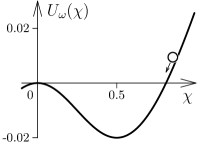
Figure 2: Mechanical potential $U_{\omega}(\chi)$ plotted for $\omega=0.8$ in the model (6).

Now, we can study the oscillons with methods developed for $Q$-balls Coleman:1985ki ; Nugaev:2019vru . We will assume that they are spherically symmetric ${\chi=\chi(r)}$: numerical simulations indeed indicate that angular asymmetry disappears immediately after formation of these objects Adib:2002ff , just like in the case of gravitationally bound Bose stars Dmitriev:2021utv . The profile equation for $\chi(r)$ takes the form,

$$\partial_{r}^{2}\chi+\frac{d-1}{r}\,\partial_{r}\,\chi=-dU_{\omega}/d\chi\;.$$ (28)

Notably, Eq. (28) coincides with the Newton’s law for a unit mass particle moving with “time” $r$ in the mechanical potential $U_{\omega}(\chi)$, see Fig. 2. The second term in Eq. (28) describes friction that decreases the mechanical energy in $d>1$. Since the oscillon is regular and localized, we impose boundary conditions $\partial_{r}\chi=0$ at $r=0$ and ${\chi\to 0}$ as ${r\to+\infty}$. This means that the analogous particle starts at $r=0$ with zero velocity and some $\chi(0)=\chi_{0}$ and arrives to ${\chi=0}$ as ${r\to+\infty}$.

It is clear that $U_{\omega}(\chi)$ should be very special for the above motion to occur, and this imposes conditions on the oscillon amplitude $\chi_{0}$, frequency $\omega$, and the scalar potential $V(\varphi)$. First, ${\chi=0}$ should be the maximum of $U_{\omega}$, or the particle would not stuck there as ${r\to+\infty}$. This simply implies

$$\omega<m\;,$$ (29)

i.e. the binding energies ${\omega-m}$ of quanta inside the oscillon are negative. Indeed, at small $\varphi$ we can approximate $V(\varphi)\approx m^{2}\varphi^{2}/2$. This gives the canonical transformation $\Phi$ of a harmonic oscillator and weak-field asymptotics of the EFT form factors,

$$\Phi\approx\sqrt{2I/m}\,\cos\theta\,,\quad h\approx mI\,,\quad\mu_{I}\approx 4Im\,,\quad U_{\omega}\approx m(\omega-m)\,\chi^{2}\quad\mbox{at small }I,\,\chi\;.$$ (30)

We see that the potential $U_{\omega}(\chi)$ has a maximum ${U_{\omega}=0}$ at ${\chi=0}$ only if the frequency is bounded from the above, $\omega<m$.

Second, the analogous particle should start its motion downhill with positive mechanical energy (${d>1}$) or with zero energy (${d=1}$); otherwise it will not reach the maximum $U_{\omega}(0)=0$. This gives necessary requirements ${\partial_{\chi_{0}}U_{\omega}(\chi_{0})>0}$ and ${U_{\omega}(\chi_{0})\geq 0}$, where $\chi_{0}\equiv\chi(0)$. In terms of the original EFT fields,

$$\omega>\Omega(I_{0})\;,\qquad\qquad\omega\geq h(I_{0})/I_{0}\;,\qquad\mbox{and}\qquad\mu_{I}(I)\neq 0\;\;\mbox{at $I\leq I_{0}$}\;,$$ (31)

where the oscillon amplitude $I_{0}=\psi_{0}^{2}$ at $r=0$ corresponds to $\chi_{0}$. Note that the “EFT mass” $\mu_{I}(I)$ is non-negative by definition (13), but may reach zero at singular points of the canonical transformation. Note also that in $d=1$ the mechanical energy is conserved and the second of Eqs. (31) turns into an equality. We see that the oscillon frequency is bounded from the below.

Together, Eqs. (29) and (31) give conditions for the oscillon with amplitude $I_{0}$ to exist in a given model:

$$\Omega(I_{0})<m\;,\qquad h(I_{0})/I_{0}<m\;,\quad\mbox{and}\quad\mu_{I}\big{|}_{I\leq I_{0}}\neq 0\qquad\mbox{for some $I_{0}$}\;.$$ (32)

In the specific case $d=1$ we obtain an additional requirement

$$\Omega(I_{0})<h(I_{0})/I_{0}\qquad\qquad\mbox{in}\quad d=1\;.$$ (33)

Now, recall that $\Omega(I)$ is the frequency of nonlinear oscillations in the potential $V(\varphi)$, and $\Omega(0)=m$. The conditions (32), mean that this frequency is smaller at ${I=I_{0}}$ than at ${I\to 0}$, and the same inequality holds for the amplitude-averaged frequency ${h(I_{0})/I_{0}=I_{0}^{-1}\int_{0}^{I_{0}}\Omega(I)\,dI}$. We obtained a precise way of saying that the potential $V(\varphi)$ is attractive in the case of strong fields. Typically, such a behavior is expected from $V(\varphi)$ which grows slower than $\varphi^{2}$ and has decreasing $\Omega(I)$.

In $(1+1)$ dimensions, the friction term in Eq. (28) is absent and the oscillon profiles can be obtained analytically. Let us illustrate this calculation in the model (6) with ${m=1}$. We substitute the respective form factors $h(I)$ and $\mu_{I}(I)$ [Eqs. (18) and (20)] into the conditions (31), (32), and (33) and find out that the oscillons do exist in this model, their central amplitudes satisfy ${0<I_{0}<1}$, and the frequencies belong to the range ${1/2<\omega<1}$. For these values, the “mechanical” potential $U_{\omega}(\chi)$ has the aforementioned specific form; it is plotted in Fig. 2 at $\omega=0.8$. Recall that the second of Eqs. (31) is an equality in one dimension. It fixes the field in the oscillon center: $\psi(0)=\sqrt{I_{0}}=\sqrt{2-2\omega}$.

     

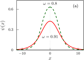
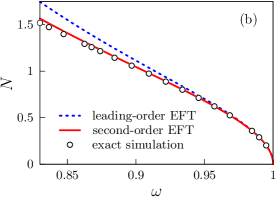
Figure 3: (a) Two leading-order EFT profiles of one-dimensional oscillons in the model (6), see Eq. (34). (b) Oscillon charges $N(\omega)$ in $d=1$ predicted by the leading-order EFT [dotted line, Eq. (35)], next-to-leading order EFT [solid line, Eq. (62)], and extracted from full numerical simulations (circles).

Solving the profile equation, we obtain an analytic and even function $\psi(x)$ in the implicit form,

$$r=\frac{2}{\sqrt{2\omega-1}}\arctan\frac{\zeta(\psi)}{\sqrt{2\omega-1}}-\frac{1}{\sqrt{2\omega}}\arctan\frac{\zeta(\psi)}{\sqrt{2\omega}}+\frac{1}{\sqrt{2-2\omega}}\;\mathrm{arctanh}\,\frac{\zeta(\psi)}{\sqrt{2-2\omega}}\;,$$ (34)

where $\zeta(\psi)=\sqrt{2-2\omega-\psi^{2}}$ and $r=|x|$ in one dimension; see Appendix C for details. Together with ${\theta=\omega t}$, this solution specifies the oscillon field $\varphi(t,\,x)=\Phi(\psi^{2},\,\theta)$ via Eq. (19). We display $\psi(x)$ in Fig. 3a (solid and dashed lines) and related $\varphi(0,\,x)$ in Fig. 4a (dotted line). Note that the oscillon with higher $\omega$ is lower in amplitude and has larger size $R$. Indeed, Eq (34) shows that $R\propto(1-\omega)^{-1/2}$ grows to infinity in the nonrelativistic limit $\omega\to 1$. In the latter case the EFT becomes exact.

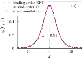
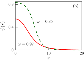
Figure 4: (a) The field $\varphi(0,\,x)$ of one-dimensional oscillon with $\omega=0.91$ in the model (6). Circles represent exact numerical simulations, dotted and solid lines are the leading-order and second-order EFT results, respectively, see Eqs. (19), (34), and (60). (b) Two leading-order EFT profiles $\psi(r)$ of three-dimensional oscillons in the model (6).

Given $\psi(r)$, we calculate the charge $N$ and energy $E$ of one-dimensional oscillons in the model (6) using Eqs. (4) and (24):

$$N=\frac{4}{\sqrt{2\omega-1}}\;\arctan\frac{\sqrt{1-\omega}}{\sqrt{\omega-1/2}}-\frac{4}{\sqrt{2\omega}}\;\arctan\sqrt{1/\omega-1}\;,$$ (35)

$$E=\frac{4(1-\omega)}{\sqrt{2\omega-1}}\;\arctan\frac{\sqrt{1-\omega}}{\sqrt{\omega-1/2}}+2\sqrt{2\omega}\;\arctan\sqrt{1/\omega-1}\;,$$ (36)

see the dotted lines in Figs. 3b and 5c, and also Appendix C for details. Notably, $E(\omega)$ and $N(\omega)$ are monotonic in $d=1$, which means that the oscillons contain more charge at larger binding energies $m-\omega$. In Sec. 5, we will see that this is no longer the case in three dimensions.

4.2 Longevity and stability

Now, we make critical remarks on longevity and stability of oscillons. One notices that the time derivative of the oscillon field in Eq. (8) equals ${\partial_{t}\varphi=\omega\,\partial_{\theta}\Phi}$ and does not coincide with the field momentum ${\pi_{\varphi}=\Pi\equiv\Omega\,\partial_{\theta}\Phi}$, where the last identity is generically valid for mechanical action-angle variables. This apparent mismatch is explained by observing that ${\omega-\Omega(I)}$ should be small for the EFT to work. Indeed, the second spatial derivative of $\psi(\boldsymbol{x})$ in Eq. (23) is proportional to $\omega-\Omega$ implying that the oscillon size is proportional to $R\propto|\omega-\Omega|^{-1/2}$. We conclude that $\Omega(I)$ should be almost constant inside the oscillon, i.e.

$$\mbox{EFT:}\qquad|d\Omega/dI|\ll\Omega/I\qquad\mbox{or}\qquad\eta^{2}\equiv|d\ln\Omega/d\ln I|\ll 1\qquad\mbox{at}\qquad I\leq I_{0}\;,$$ (37)

where $I_{0}$ is the amplitude in the center. Moreover, one crudely expects ${(mR)^{-2}\sim|d\ln\Omega/d\ln I|}$ because $\Omega-\omega\propto\partial_{I}\Omega$, cf. Eq. (23). Note that we can relax Eq. (37) a bit, e.g., by imposing it at $I_{1}<I\leq I_{0}$, where $I_{1}\ll I_{0}$. In this case the EFT works only in the oscillon core ${I>I_{1}}$, and the entire object slowly evaporates through the boundaries.

Importantly, we expect the oscillons to live longer if Eq. (37) is satisfied to a better precision. Indeed, charge conservation prohibits their decay in the approximate EFT and, as we will see in Sec. 7, higher-order EFT corrections do not ruin this property. Hence, the oscillon lifetimes are large — presumably, exponentially large — in the expansion parameter $\eta\ll 1$. This turns Eq. (37) into a condition for the oscillon longevity.

So far, we formulated all requirements in terms of mechanical oscillation frequency $\Omega$ in the scalar potential $V(\varphi)$. But once the appropriate $\Omega(I)$ is found, one can restore ${\varphi\to-\varphi}$ symmetric potential using the identity LL1 ,

$$\varphi(V)=\int_{0}^{V}\frac{dh}{\Omega(h)\sqrt{2V-2h}}\;,$$ (38)

where $\varphi(V)$ is the inverse to $V(\varphi)$ and $\Omega$ in the right-hand side is expressed in terms of the “mechanical energy” $h(I)$. In particular, Eq. (37) suggests that the scalar potential is nearly quadratic.

Let us discuss two obvious ways to satisfy all requirements. First, the EFT always applies in the limit $I\to 0$ if $\partial_{I}\Omega(0)$ is finite and nonzero. Indeed, any smooth potential $V(\varphi)$ is almost quadratic near the vacuum. The respective oscillons are long-lived and large in size: ${R\sim|mI_{0}\partial_{I}\Omega(0)|^{-1/2}\propto I_{0}^{-1/2}}$, where the parameter in Eq. (37) was exploited. Besides, due to Eqs. (29) and (31) their frequencies are slightly below the field mass, $m-\omega\propto I_{0}$. Finally, the conditions (32) for the existence of these objects fix the sign ${\partial_{I}\Omega(0)<0}$.

A suitable technique working at $I\to 0$ alongside the EFT is the small-amplitude approximation Dashen:1975hd ; Kosevich1975 ; Fodor:2008es ; Fodor:2019ftc . In this case one Taylor-expands all quantities in $I$ and $\varphi$. In particular, the series for $\Omega(I)$ in Eq. (38) give,

$$V=\frac{1}{2}m^{2}\varphi^{2}+\frac{g_{3}}{4}\,\varphi^{4}+\frac{g_{5}}{6}\,\varphi^{6}+\dots\;,$$ (39)

where $g_{3}=\frac{4}{3}m^{2}\partial_{I}\Omega(0)<0$ and the dots are terms with higher powers of $\varphi$. Apart from the necessarily negative four-coupling $g_{3}$, this potential is generic — hence, small-amplitude oscillons appear in all models with attractive self-interactions. But notably, Eq. (39) is not applicable for strong fields. This is tolerable if Eq. (37) is not satisfied at large $I$ and if large-amplitude oscillons decay faster. Our illustrative potential (6) with $\Omega=1-I$ and ${m=1}$ is an example for that. However, there exist other cases to consider.

Second, in certain specifically chosen models $\Omega(I)$ may be flat even for finite $I$. In this case the small-amplitude expansion is not applicable. Let us take $\Omega=\Omega_{0}+\delta\Omega(I)$, where $\Omega_{0}$ is a constant and the function ${\delta\Omega(I)\ll\Omega_{0}}$ is either bounded at large $I$ or grows logarithmically. Then the EFT condition (37) is satisfied. Expanding Eq. (38) in $\delta\Omega$, we arrive to

$$V=\frac{1}{2}\tilde{\Omega}^{2}(\varphi)\,\varphi^{2}\;,\qquad\mbox{with}\qquad\tilde{\Omega}^{2}\approx\Omega_{0}^{2}+\frac{2}{\varphi}\int\limits_{0}^{\Omega_{0}^{2}\varphi^{2}/2}\frac{dh\,\delta\Omega(h)}{\sqrt{\Omega_{0}^{2}\varphi^{2}-2h}}\;.$$ (40)

This potential is almost quadratic since $\tilde{\Omega}(\varphi)$ is nearly constant and grows at best logarithmically at large $\varphi$. Notably, Eq. (40) includes monodromy potentials in Olle:2019kbo ; Olle:2020qqy which are already known to support exceptionally long-lived large-amplitude oscillons. Our estimates show that the size of the latter objects and their lifetimes can be controlled by the parameter (37), cf. Ref. Olle:2019kbo .

Next, we consider linear stability of oscillons. One generically expects Amin:2010jq that these objects are destroyed by long-range perturbations if Vakhitov-Kolokolov criterion vk ; Zakharov12 is broken;

$$\mbox{stability:}\quad dN(\omega)/d\omega=\omega^{-1}\;dE(\omega)/d\omega<0\;.$$ (41)

In the EFT, we rigorously prove this criterium in the simplest possible way vk ; Zakharov12 , by demonstrating that the oscillons can be the true minima of energy at a fixed $N$ only if Eq. (41) is satisfied. We present the proof in Appendix D. Note that one-dimensional oscillons in the model (6) do satisfy the stability criterion (41), see Fig. 3b.

One bewares Amin:2010jq ; Olle:2020qqy that certain oscillons may decay via parametric resonance Tkachev:1987cd ; Levkov:2020txo for high-frequency modes that are discarded in the EFT. Certain intuition may even suggest that this mechanism is efficient for large-size and high-amplitude objects, i.e. precisely in the EFT case. Let us argue that, to the contrary, parametric resonance is suppressed whenever the EFT condition (37) holds. Indeed, deep inside the oscillons high-frequency perturbations $\delta\varphi$ with wave vectors ${k\sim O(m)}$ satisfy the equation [cf. Eq. (5)],

$$(\partial_{t}^{2}+k^{2})\delta\varphi=-V^{\prime\prime}(\Phi(I_{0},\,\omega t))\,\delta\varphi\;,$$ (42)

where the primes denote derivatives with respect to $\varphi$ and we ignored slow dependence on $\boldsymbol{x}$ in $I(\boldsymbol{x})\approx I_{0}$. In the infinite medium, the periodic oscillations of ${V^{\prime\prime}}$ would always excite the modes inside some resonance $k$-bands of width $\delta k\sim|V^{\prime\prime}_{\mathrm{osc}}|/k$, where Eq. (42) was used in the estimate and the subscript “osc” denotes the oscillatory part of $V^{\prime\prime}$, cf. LL1 . This makes $\delta\varphi(t,\,\boldsymbol{k})$ grow exponentially within the bands. Instabilities in compact objects, however, cannot develop unless the growing modes can be localized inside them. We obtain a crude condition for the parametric instability Tkachev:1987cd ; Levkov:2020txo : ${\delta k\gtrsim R^{-1}}$ or ${R|V^{\prime\prime}_{\mathrm{osc}}|\gtrsim m}$, where $R$ is the oscillon size. However, the EFT condition (37) ensures that the scalar potential is almost quadratic with suppressed oscillations of $V^{\prime\prime}$. We obtain ${(mR)^{-2}\sim|d\ln\Omega/d\ln I|\propto|V^{\prime\prime}_{\mathrm{osc}}/m^{2}|}$ and therefore small $R|V^{\prime\prime}_{osc}|/m\propto(mR)^{-1}\ll 1$. Thus, parametric instability is not expected to occur if Eq. (37) is satisfied, see also Olle:2020qqy .

5 Application and numerical tests

In two and three dimensions, the EFT profiles of oscillons $\psi(r)$ cannot be found analytically, so we compute them numerically in the model (6). To this end we use the shooting method. The result in $d=3$ is plotted in Fig. 4b. As expected, the profiles are lower and larger in size if $\omega$ is closer to $m=1$, and the same property holds in two dimensions.

The energies $E(\omega)$ of the EFT oscillons in various $d$ are plotted with dotted lines in Figs. 5a, b, and c, see Eqs. (24) and (4). One observes a striking feature: $dE/d\omega$ is positive in the right-hand side of the three-dimensional graph. This means that the criterion (41) is broken at ${\omega\approx m}$, $d=3$ and the respective oscillons are unstable. Sadly, this happens precisely in the region where both the EFT and small-amplitude expansion work best.

In fact, oscillons with small amplitudes are generically unstable in ${d\geq 3}$ dimensions. Indeed, in Sec. 4.2 we estimated their sizes $R\propto 1/\sqrt{I_{0}}$ and frequencies ${m-\omega\propto I_{0}}$ in terms of the central amplitudes $I_{0}$. This parametrically fixes their charges ${N(\omega)\propto R^{d}I_{0}\propto(m-\omega)^{1-d/2}}$ and energies $E\approx mN$, see Eqs. (4) and (25). Thus, at ${\omega\to m}$ the oscillon parameters $E$ and $N$ universally tend to zero, remain constant, or grow to infinity in $d=1$, $2$, and $d\geq 3$ dimensions, respectively. The stability criterion is broken at $\omega\approx m$ in ${d\geq 3}$.

Now, we compare predictions of the leading-order EFT with exact numerical results in the model (6). We perform spherically-symmetric simulations for $\varphi(t,\,r)$ like in Sec. 2, but start from the approximate EFT oscillons in Eq. (19), where the profiles $I=\psi^{2}(r)$ are computed above and $t=\theta=0$. The latter configurations settle faster into the actual oscillons than the Gaussian initial data. We wait at least $10^{3}$ oscillation cycles for that to happen. Then we compute the periods $T$ of the equilibrated objects as the average time intervals between the consecutive maxima of $\varphi(t,\,0)$. The oscillon frequencies are ${\omega=2\pi/T}$, their energies are computed as

$$E=\int\limits d^{d}\boldsymbol{x}\,\left[(\partial_{t}\varphi)^{2}/2+(\partial_{i}\varphi)^{2}/2+V(\varphi)\right]\;,$$ (43)

and the charges $N$ are given by Eq. (17). Starting from various EFT profiles, we obtain oscillons with different frequencies and functions $E(\omega)$, $N(\omega)$.

In Appendix A we describe details of the above numerical procedure, perform tests and estimate numerical errors (which are small). One technical trick deserves to be mentioned in the main text. In long simulations, we absorb all outgoing radiation in order to prevent its reflection from the boundaries onto the central object. This is achieved by using the “artificial damping” of Ref. Gleiser:1999tj . Namely, we modify Eq. (5) to

$$\left(\partial^{2}_{t}+H(r)\partial_{t}-\Delta\right)\varphi=-V^{\prime}(\varphi)\;,$$ (44)

where the “sponge” function $H(r)$ equals zero in the main part $r<R_{s}$ of the lattice and smoothly increases at the lattice boundaries. Equation (44) describes field in de Sitter Universe with $r$-dependent Hubble constant $H(r)/3$. In this setting, the outgoing scalar waves fade out exponentially at ${r>R_{s}}$ like in the expanding Universe, while the dynamics in the lattice center remains unmodified. This strategy allows us to control oscillons in long runs.

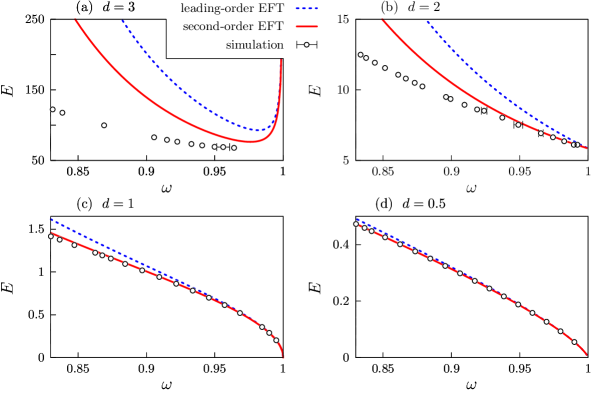
Figure 5: The energy $E(\omega)$ of $d$-dimensional oscillons in the leading-order EFT (dotted lines) and second-order EFT (solid lines). Circles with errorbars show results of exact numerical simulations.

The simulation results for $N(\omega)$ in $d=1$ dimension and $E(\omega)$ in $d=1$, $2$, and $3$ are shown in Figs. 3b and 5a, b, c with circles. The errorbars represent numerical uncertainties whenever they exceed the circle size. One observes that the predictions of the leading-order EFT (dotted lines in the figures) coincide with the exact results at $\omega\approx m=1$ but deviate from them at lower $\omega$, as can be expected from the criterion (37). The only exception is the case $d=3$ in Fig. 5a where the simulations cannot produce unstable oscillons with $\omega>0.97$, and the agreement in the rest of the $\omega$ region is qualitative.

In Sec. 4.2 we have made an important suggestion that the oscillons live exponentially long whenever the EFT applies. In other words, the emission rate $\Gamma$ of these objects is expected to have the form

$$\Gamma\equiv|E^{-1}\partial_{t}E|\sim\varsigma_{1}\,\mathrm{e}^{-\varsigma_{2}/\eta}\,,$$ (45)

where $\eta\equiv|d\ln\Omega/d\ln I|^{1/2}\sim(mR)^{-1}$ is the EFT expansion parameter, $I=I(0)$ is the oscillon amplitude at $r=0$, and $\varsigma_{i}$ are constants. Note that expression similar to Eq. (45) was derived analytically in the special case of small-amplitude objects Segur:1987mg ; Fodor:2008du ; Fodor:2009kf . We confirm it by computing the rates $\Gamma(\omega)$ of three-dimensional oscillons in full simulations, see the lines-points in Fig. 6 (logarithmic scale). It is clear that the data in the right part of this graph are correctly described by the exponent (45) (solid line), where the best-fit parameters are $\ln(\varsigma_{1}/m)=-5.55\pm 0.38$ and ${\varsigma_{2}=7.02\pm 0.34}$ and $\eta=\sqrt{I/(1-I)}$ in our model. We conclude that emission of oscillons is indeed exponentially small at ${\eta\ll 1}$, and this corresponds to the regime $\omega\approx 1$ in our model.

At smaller $\omega$ extremely long-lived oscillons with $\eta\sim O(1)$ appear. They are not controlled by the EFT and deserve further study. Note that similar non-monotonic dependences of emission rates were observed in Zhang:2020bec ; Olle:2020qqy ; Cyncynates:2021rtf .

Figure 6: Decay rate $\Gamma(\omega)=E^{-1}\partial_{t}E$ of three-dimensional oscillons as a function of frequency in the model (6) (circles with an interpolating dashed line in the logarithmic scale). Solid line is the fit (45).

One sees another remarkable feature of Figs. 5a, b, and c: EFT works significantly better in lower dimensions. Indeed, it reproduces exact results qualitatively in $d=3$ but becomes almost precise for a range of frequencies in $d=1$. To test this property, we notice that $d$ enters as a parameter into the spherically-symmetric equations for $\varphi(t,\,r)$ and $\psi(r)$. Hence, we can formally perform numerical calculations in non-integer $d$. In Fig. 5d we compare full simulations (circles) with the leading-order EFT (dotted line) in ${d=0.5}$ and find almost perfect coincidence. This suggests that the leading-order EFT becomes exact in the formal limit $d\to 0$. In the next Section we will find out why.

6 The limit of zero dimensions

Now, we argue that oscillons turn into ever-lasting and exactly periodic solutions in the formal limit $d\to 0$. This explains why they are more common Gleiser:2004an in lower dimensions.

We analytically continue the spherically-symmetric field equation

$$\partial^{2}_{t}\varphi-\partial^{2}_{r}\varphi-\frac{d-1}{r}\,\partial_{r}\varphi=-V^{\prime}(\varphi)$$ (46)

to fractional $d$ imposing regularity condition $\partial_{r}\varphi=0$ at the origin ${r=0}$. The latter requirement guarantees that ${\varphi=\varphi_{0}(t)+\varphi_{2}(t)\,r^{2}+O(r^{4})}$ at small $r$. Substituting the expansion into Eq. (46) and setting $r=0$, we obtain equation for the first two coefficients:

$$\partial_{t}^{2}\varphi_{0}-2\varphi_{2}d=-V^{\prime}(\varphi_{0})\;.$$ (47)

Notice that precisely in $d=0$ the field in the center $\varphi_{0}(t)$ satisfies a mechanical equation which is independent from the rest of the evolution. This agrees with the intuitive interpretation of a zero-dimensional field as a mechanical pendulum $\varphi_{0}(t)$ oscillating in the potential $V(\varphi)$. In our spherically-symmetric system the pendulum imposes time-periodic Dirichlet boundary condition $\varphi(t,\,0)=\varphi_{0}(t)$ on the field in the bulk. Regardless of the initial data, the bulk configuration should eventually settle into a stationary configuration oscillating with a period of the external force $\varphi_{0}(t)$. We thus constructed an eternal exactly periodic solution in $d=0$, a prototype for the lower-dimensional oscillons.

To see the periodic solution explicitly, we numerically solve Eq. (46) with $d=0$ in the model (6). As before, this evolution starts from the approximate EFT profile, say, with ${\omega=0.65}$. After a stage of irregular wobbling, the solution enters the stationary regime with exact period $2\pi/\omega$, and stays there to the very end of the simulation at ${t\approx 2\cdot 10^{5}}$, see Fig. 7a.

Consider now the limit $d\to 0$ of the integral quantities, e.g. the energy (43). We write the volume element as $d^{d}\boldsymbol{x}=S_{d-1}(\mu r)^{d}\,dr/r$, where ${S_{d-1}=2\pi^{d/2}/\Gamma(d/2)}$ is the area of a unit sphere and the scale $\mu$ is introduced to fix the mass dimension of the integrand. Notably, ${S_{d-1}\to 0}$ in the zero-dimensional limit. In the total volume this multiplier is compensated by the radial integral which diverges logarithmically near $r=0$ in $d=0$. As a consequence, all volume integrals in small $d$ receive main contributions near the origin. In particular, the energy (43) takes the form,

$$E=E_{0}+E_{1}d+O(d^{2})\;,\quad E_{0}=(\partial_{t}\varphi_{0})^{2}/2+V(\varphi_{0})\;,\quad E_{1}=\int_{\epsilon}^{\infty}\rho\,dr/r+E_{0}\ln(c\mu\epsilon)$$

where $\rho(r)$ is the integrand in Eq. (43), $c=\mathrm{e}^{\gamma_{E}/2}\sqrt{\pi}\approx 2.37$ is a number involving the Euler constant $\gamma_{E}$, and the limit $\epsilon\to+0$ is assumed. We see, quite expectedly, that at small $d$ the leading contribution comes from the pendulum energy $E_{0}$ in the center, while the bulk part $E_{1}d$ is suppressed.

Nevertheless, the bulk energy is conserved even in $d=0$. In this case Eq. (46) gives $\partial_{t}E_{1}=J_{0}-J$, where $J=-\lim\limits_{r\to\infty}r^{-1}\partial_{t}\varphi\partial_{r}\varphi$ is the flux radiated to infinity and $J_{0}=-\partial_{t}\varphi\partial^{2}_{r}\varphi\big{|}_{r=0}$ comes from the origin. In Fig. 7b we plot the period-averaged flux $\langle J\rangle$ for the solution in Fig. 7a. After several oscillations, it approaches a constant value $J_{\infty}$ indicating a stationary regime. We conclude that $\varphi_{0}$ oscillator sends $O(d)$ stationary energy flux through the bulk to infinity.

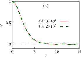
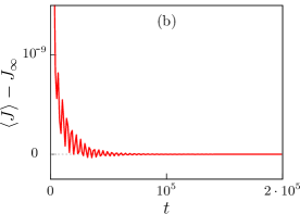
Figure 7: Numerical solution of Eq. (46) with $d=0$ in the model (6). The simulation starts from the approximate EFT oscillon with $\omega=0.65$ and amplitude $\varphi(0,0)\approx 1$ in the center. (a) Field configurations $\varphi(t,\,r)$ at two essentially different time moments that both correspond to ${\partial_{t}\varphi(t,\,0)=0}$. (b) Energy flow $\langle J\rangle=-r^{-1}\langle\partial_{t}\varphi\partial_{r}\varphi\rangle$ at ${r=50}$ averaged over several oscillation periods; we subtracted the asymptotic value $\langle J\rangle\to J_{\infty}\approx 1.0088\cdot 10^{-5}$ as $t\to+\infty$.

It is already clear that our effective theory becomes exact in the limit $d\to 0$. Indeed, we introduced $I$ and $\theta$ as the action and angle variables in the mechanical system with potential $V(\varphi)$. In $d=0$, the EFT solution with $I(0)=I_{0}$ and $\theta=\omega t$ exactly describes motion of the $\varphi_{0}$ pendulum at $r=0$. Moreover, the profile equation (23) reduces at $r=0$ to $\Omega(I_{0})=\omega$ i.e. fixes the pendulum frequency to $\omega$. As a result, all corrections to the leading-order EFT come from the bulk, and they are proportional to $d$. This is the reason why the EFT is more precise in lower dimensions.

7 Higher-order corrections

In this Section, we evaluate EFT corrections and demonstrate that full effective action has the form of a systematic gradient expansion, where every other term is suppressed as $(mR)^{-2}$ with respect to the previous one. To make the technicalities more transparent, we illustrate them in a toy model in Appendix B.

By itself, the transformation from $\pi_{\varphi}$, $\varphi$ to $I$, $\theta$ leaves the theory exact. The main approximation of the leading-order EFT is the assumption that the latter fields change slowly in space and time. In the second order, we split them into smooth and fast-oscillating parts:

$$I=\bar{I}+\delta I\;,\qquad\qquad\theta=\bar{\theta}+\delta\theta\;,$$ (48)

where the perturbations have zero period averages, $\langle\delta I\rangle=\langle\delta\theta\rangle=0$, so that ${\langle I\rangle=\bar{I}}$ and ${\langle\partial_{t}\theta\rangle=\partial_{t}\bar{\theta}}$. Below we will see that $\delta I$ and $\delta\theta$ are small in the EFT expansion parameters. We will be able to evaluate them perturbatively.

Now, the true EFT fields are $\bar{I}$, $\bar{\theta}$ and their combination $\psi=\sqrt{\bar{I}}\cdot\mathrm{e}^{-i\bar{\theta}}$. An effective action for them can be obtained by substituting the solutions for $\delta I$ and $\delta\theta$ into the exact action,

$${\cal S}=\int dtd^{d}\boldsymbol{x}\left[I\partial_{t}\theta-h(I)+\Phi\Delta\Phi/2\right]\;,$$ (49)

where the canonical transformation $\varphi=\Phi(I,\,\theta)$ was inserted into Eq. (11). Varying Eq. (49) and subtracting the period-averaged equations, we arrive to equations for perturbations,

$$\partial_{t}\delta I=j_{\theta}(I,\,\theta),\qquad\qquad\partial_{t}\delta\theta=\Omega(I)-\langle\Omega\rangle-j_{I}(I,\,\theta)\;,$$ (50)

where, as usual, $\Omega=\partial_{I}h$, and we introduced the sources

$$j_{\theta}=\partial_{\theta}\Phi\,\Delta\Phi,\qquad\qquad j_{I}=\partial_{I}\Phi\,\Delta\Phi-\langle\partial_{I}\Phi\,\Delta\Phi\rangle$$ (51)

depending on $I=\bar{I}+\delta I$ and $\theta=\bar{\theta}+\delta\theta$. We see that $\delta I$ and $\delta\theta$ are small, indeed: in Eqs. (50) they are determined by $j_{I}$ and $j_{\theta}$ which include two spatial derivatives and hence are suppressed as $(mR)^{-2}$.

In the second-order EFT, we solve for $\delta I$ and $\delta\theta$ in the leading order. In this case the time derivatives in Eqs. (50) can be changed to ${\partial_{t}\approx(\partial_{t}\bar{\theta})\,\partial_{\bar{\theta}}}$, since $\bar{\theta}$ evolves progressively during the oscillation period. Also, we can expand ${\Omega-\langle\Omega\rangle\approx\delta I\cdot\partial_{\bar{I}}\Omega}$ and ignore the perturbations in $j_{\theta}$ and $j_{I}$. This gives,

$$\delta I\approx\frac{{\cal I}[j_{\theta}(\bar{I},\,\bar{\theta})]}{\partial_{t}\bar{\theta}}\;,\qquad\qquad\delta\theta\approx\frac{1}{\partial_{t}{\bar{\theta}}}\,\Big{\{}\partial_{\bar{I}}\Omega(\bar{I})\,{\cal I}[\delta I(\bar{I},\,\bar{\theta})]-{\cal I}[j_{I}(\bar{I},\,\bar{\theta})]\Big{\}}\;,$$ (52)

where we introduced a natural primitive on the $\bar{\theta}$ circle for functions with zero average,

$${\cal I}[f]=\int_{0}^{\bar{\theta}}f(\bar{\theta}^{\prime})\,d\bar{\theta}^{\prime}-\Big{\langle}\int_{0}^{\bar{\theta}}f(\bar{\theta}^{\prime})\,d\bar{\theta}^{\prime}\;\Big{\rangle}\qquad\mbox{satisfying}\quad\langle{\cal I}[f]\rangle=\langle f\rangle=0\;.$$ (53)

From now on, the period averages $\langle\cdot\rangle$ are given by complete integrals over $\bar{\theta}$, like in Eq. (12).

It is remarkable that Eqs. (52) express perturbations in terms of the EFT fields $\bar{I}(t,\,\boldsymbol{x})$ and $\bar{\theta}(t,\,\boldsymbol{x})$ which are arbitrary. Expanding Eq. (49) in $\delta I$ and $\delta\theta$ and substituting the above solutions, we arrive to the second-order effective action ${\cal S}\approx{\cal S}_{\mathrm{eff}}^{(1)}+{\cal S}_{\mathrm{eff}}^{(2)}$, where ${\cal S}_{\mathrm{eff}}^{(1)}[\bar{I},\,\bar{\theta}]$ is the leading-order result in Eq. (14) and the correction is

$${\cal S}_{\mathrm{eff}}^{(2)}[\bar{I},\,\bar{\theta}\,]=\int dt\,d^{d}\boldsymbol{x}\left[\frac{1}{\partial_{t}\bar{\theta}}\left\langle j_{I}\mathcal{I}[j_{\theta}]\right\rangle-\frac{\partial_{\bar{I}}\Omega}{2(\partial_{t}\bar{\theta})^{2}}\langle\left(\mathcal{I}[j_{\theta}]\right)^{2}\rangle\right]\;,$$ (54)

see Appendix E.1 for the detailed derivation. It is worth noting that $j_{\theta}$ and $j_{I}$ in this expression already depend on $\bar{I}$ and $\bar{\theta}$.

Let us make three important observations. First, the time integral in the action effectively averages the Lagrangian over the oscillation period. This can be done by integrating over $\bar{\theta}$, so we added overall period averages to every term of Eq. (54). As a consequence of the averaging, the second-order EFT retains shift symmetry $\bar{\theta}\to\bar{\theta}+\alpha$, and a conserved charge

$$N=\int d^{d}\boldsymbol{x}\left[\bar{I}+\frac{\delta{\cal S}_{\mathrm{eff}}^{(2)}}{\delta(\partial_{t}\bar{\theta})}\right]\;,$$ (55)

cf. Eq. (4). This again guarantees that the stationary Ansatz $\bar{\theta}=\omega t$ and $\bar{I}=\bar{I}(\boldsymbol{x})$ passes the effective equations: nontopological solitons — oscillons — exist in the next-to-leading order.

Second, the correction (54) has $\partial_{t}\bar{\theta}$ in the denominator — hence, EFT works for oscillons with $\omega\sim m$, but not for static fields. Third, there are four spatial derivatives of $\bar{I}$ and $\bar{\theta}$ in every term of ${\cal S}_{\mathrm{eff}}^{(2)}$, they are hidden inside $j_{\theta}$ and $j_{I}$. One can see this explicitly: substitute the sources (51), expand the derivatives $\Delta\Phi(\bar{I},\,\bar{\theta})$, move smooth quantities like $\partial_{i}\bar{I}$ or $\partial_{i}\bar{\theta}$ outside of the period averages, and integrate the remaining coefficients in the effective Lagrangian over $\bar{\theta}$. In Appendix E.2 we perform this calculation in the simplified case of oscillon with $\partial_{i}\bar{\theta}=0$ and $\bar{I}=\psi^{2}(\boldsymbol{x})$. The result is

$${\cal S}^{(2)}_{\mathrm{eff}}=-\int dt\,F^{(2)}\,,\qquad F^{(2)}=-\int d^{d}{\boldsymbol{x}}\left[d_{1}\,(\partial_{i}\psi)^{4}+d_{2}\,\psi\Delta\psi(\partial_{i}\psi)^{2}+d_{3}\,(\Delta\psi)^{2}\right]\,,$$ (56)

where $-F^{(2)}$ is a correction to the Lagrangian and the form factors $d_{i}$ depend on $\psi^{2}$. Say,

$$d_{3}(\psi^{2})=\left.\frac{4\bar{I}}{\omega}\,\langle\,(\partial_{\bar{I}}\Phi)^{2}\,{\cal I}[\partial_{\bar{\theta}}\Phi\partial_{\bar{I}}\Phi]\,\rangle-\frac{2\bar{I}}{\omega^{2}}\,\partial_{\bar{I}}\Omega\,\langle\,\left({\cal I}[\partial_{\bar{\theta}}\Phi\partial_{\bar{I}}\Phi]\right)^{2}\,\rangle\right|_{\bar{I}=\psi^{2}}\;,$$ (57)

see Appendix E.1 for other coefficients. In any concrete model, the function $\Phi(\bar{I},\,\bar{\theta})$ is known, so one can evaluate integrals over $\bar{\theta}$. Analytic expressions for $d_{i}(\psi^{2})$ in the model (6) are given in Appendix E.2.

As before, we determine the oscillon profile $\bar{I}\equiv\psi^{2}(\boldsymbol{x})$, $\bar{\theta}=\omega t$ by extremizing the (minus) Lagrangian,

$$F=F^{(1)}+F^{(2)}=E-\omega N\;,$$ (58)

where the leading-order part $F^{(1)}[\bar{I}\,]$ and correction $F^{(2)}[\bar{I}\,]$ are given by Eqs. (24) and (56), respectively. The last identity in Eq. (58) follows from the general expression for energy and Eq. (55). Notably, the profile can be computed perturbatively. One writes ${\bar{I}=\bar{I}^{(1)}+\bar{I}^{(2)}}$, where $\bar{I}^{(1)}$ extremizes $F^{(1)}$ and hence solves Eq. (23), and the correction $\bar{I}^{(2)}$ satisfies linear equation

$$\frac{\delta^{2}F^{(1)}}{\delta\bar{I}^{2}}\cdot\bar{I}^{(2)}=-\frac{\delta F^{(2)}}{\delta\bar{I}}$$ (59)

in the background of $\bar{I}^{(1)}$. Once the profile is found, the oscillon field is given by Eq. (8):

$$\varphi(t,\,\boldsymbol{x})=\Phi\left(\bar{I}+\delta I(\bar{I},\,\omega t),\,\omega t+\delta\theta(\bar{I},\,\omega t)\right)\;.$$ (60)

Here $\delta I$ and $\delta\theta$ are provided by Eqs. (52) and $\bar{I}$ is the sum of $\bar{I}^{(1)}$ and $\bar{I}^{(2)}$.

To illustrate calculation of the second-order oscillon field, we numerically solved ${d=1}$ equations for $\bar{I}^{(1)}(x)$ and $\bar{I}^{(2)}(x)$ in the model (6) using the EFT form factors in Appendix E.2. The second-order EFT field $\varphi(0,\,x)$ of one-dimensional oscillon with $\omega=0.91$ is plotted in Fig. 4a (solid line). As expected, it is closer to the exact numerical result (circles) than the first-order EFT prediction (dotted line).

It is worth noting that the mismatch between the derivative $\partial_{t}\varphi$ and canonical momentum $\pi_{\varphi}\approx\partial_{t}\varphi$ of the oscillon is alleviated in the second-order EFT. Indeed, taking the time derivative of Eq. (60) and using Eqs. (52) and (23), one obtains $\partial_{t}\varphi$ which is just $O(mR)^{-4}$ different from the momentum $\pi_{\varphi}$ in Eq. (8). Recall that $\partial_{t}\varphi-\pi_{\varphi}\sim O(mR)^{-2}$ in the leading-order EFT — hence, these quantities coincide with increasing precision in higher orders.

On does not need the above corrections $\bar{I}^{(2)}$ and $\delta I$ for calculation of the second-order oscillon energy $E(\omega)$ and charge $N(\omega)$. Indeed, the leading-order profile $\bar{I}^{(1)}$ extremizes $F^{(1)}$ implying

$$F[\,\bar{I}^{(1)}+\bar{I}^{(2)}\,]=F^{(1)}[\,\bar{I}^{(1)}\,]+F^{(2)}[\,\bar{I}^{(1)}\,]+O(\,\bar{I}^{(2)}\,)^{2}+O(\,\delta_{\bar{I}}F^{(2)}\,\bar{I}^{(2)}\,)\;,$$ (61)

where both omitted terms are smaller than the next correction to the effective action with six derivatives. Once $F(\omega)$ is obtained, Eqs. (25) and (58) give other oscillon parameters,

$$N=-\partial_{\omega}{F}[\bar{I}^{(1)}]\;,\qquad\qquad E=F[\bar{I}^{(1)}]+\omega N\;,$$ (62)

which do not depend on $\bar{I}^{(2)}$ as well. In practice, the $\omega$ derivative is computed numerically.

The charges $N(\omega)$ and energies $E(\omega)$ of the second-order EFT oscillons in the model (6) are shown with solid lines in Figs. 3b and 5. They are closer to the results of exact simulations (circles) than the leading-order predictions (dotted lines), and significantly so — in lower dimensions and at $\omega\approx 1$.

We finish this Section by remarking that the subsequent EFT corrections can be calculated in the same way as the second-order one. In the third order, one breaks the perturbations $\delta I=\delta I^{(2)}+\delta I^{(3)}$ and $\delta\theta=\delta\theta^{(2)}+\delta\theta^{(3)}$ into the leading parts ${\delta I^{(2)},\;\delta\theta^{(2)}\sim O(mR)^{-2}}$ given by Eqs. (52) and even smaller corrections ${\delta I^{(3)},\;\delta\theta^{(3)}\sim O(mR)^{-4}}$. The latter are evaluated using Eqs. (50) in the respective order; notably, the resulting expressions will include squares of the sources and hence four derivatives. Plugging the refined perturbations into the exact action (49), one arrives at the next correction to the effective Lagrangian with six derivatives. Importantly, the latter also should be averaged over period, i.e. integrated over $\bar{\theta}$. This means that $\bar{\theta}\to\bar{\theta}+\alpha$ remains a symmetry at any EFT order.

8 Comparison with small-amplitude expansion and automation

We have already argued in Sec. 4 that the sizes $R$ of oscillons grow and the amplitudes $I_{0}$ become small when their frequencies approach the field mass, $\omega\to m$. Namely, $R\sim O(\epsilon^{-1})$, $I_{0}\sim O(\epsilon^{2})$, and $\varphi\sim O(\epsilon)$ in terms of a small parameter $\epsilon^{2}=m^{2}-\omega^{2}$. In this case both EFT and small-amplitude (nonrelativistic) expansion are applicable. The purpose of the present Section is therefore twofold. On the one hand, we will demonstrate that all small-amplitude results can be restored by re-expanding the effective action in the field strength to the respective order. On the other hand, we will see that the EFT can be realistically implemented in any model by symbolically computing long small-amplitude series for the form factors and summing them up numerically.

With these purposes in mind, we consider a generic scalar potential (39) in units with $m=1$. The starting point of the EFT is to introduce the mechanical action-angle variables in the potential $V(\varphi)$. They can be evaluated automatically in the form of half-integer series

$$\Phi=\sqrt{2I}\,\cos\theta+(2I)^{3/2}\,\frac{g_{3}}{32}\left[\,\cos(3\theta)-6\cos\theta\,\right]+\dots\,,\quad h=I+\frac{3}{8}g_{3}I^{2}+\gamma_{3}I^{3}+\dots\,,$$ (63)

where the dots denote higher-order contributions, $g_{i}$ are the coefficients of the potential (39), and we defined $\gamma_{3}\equiv\frac{5}{12}\,g_{5}-\frac{17}{64}\,g^{2}_{3}$. Recall that $\Omega=\partial_{I}h$ and $\Pi=\Omega\,\partial_{\theta}\Phi$. Given the representation (63), we calculate all $\theta$ integrals in the EFT form factors. In particular,

$$\frac{1}{\mu_{I}}=\frac{1}{4I}-\frac{9}{16}\,g_{3}+O(I)\;,\qquad\qquad d_{3}=\frac{1}{8\omega}+O(I)\;,$$ (64)

where Eqs. (13) and (57) were exploited. Unlike in the previous Section, now we use $I$ and $\theta$ for smooth EFT fields, omitting the overbar. It is clear that arbitrarily long series for the EFT form factors can be symbolically computed using the series for $\Phi$.

Next, we use the EFT to obtain small-amplitude expansion for the oscillon with ${I=\psi^{2}(\boldsymbol{x})}$, ${\theta=\omega t}$, and $\omega\approx 1$. We substitute the series (64) into the second-order effective Lagrangian (24), (56) and reshuffle its terms according to the power-counting in ${\epsilon\ll 1}$,

$$F^{(1)}+F^{(2)}=\int d^{d}\boldsymbol{x}\left\{\frac{1}{2}\,(\partial_{i}\psi)^{2}+\frac{\epsilon^{2}}{2}\,\psi^{2}+\frac{3}{8}\,g_{3}\psi^{4}\right.\\ \left.-\frac{9}{8}\,g_{3}\psi^{2}(\partial_{i}\psi)^{2}+\frac{\epsilon^{4}}{8}\,\psi^{2}+\gamma_{3}\psi^{6}-\frac{1}{8}\,(\Delta\psi)^{2}+O(\epsilon^{8})\right\}\;,$$ (65)

where the first and second lines are $O(\epsilon^{4})$ and $O(\epsilon^{6})$, respectively, since $\psi=O(\epsilon)$, ${\partial_{i}\psi\sim O(\epsilon^{2})}$, and $1-\omega\approx\epsilon^{2}/2+\epsilon^{4}/8$. As before, the oscillon profile can be found by varying Eq. (65) with respect to $\psi(\boldsymbol{x})$. This time, we evaluate it perturbatively in $\epsilon$, i.e. search for solution in the form,

$$\psi=\frac{\epsilon}{\sqrt{2}}\,p_{1}(\boldsymbol{x})+\frac{\epsilon^{3}}{4\sqrt{2}}\left[4p_{3}(\boldsymbol{x})-p_{1}(\boldsymbol{x})\right]+O(\epsilon^{5})\;,$$ (66)

where $p_{1}$ and $p_{3}$ control the leading-order and second-order contributions, respectively. In the first two orders, we obtain equations

$$\epsilon^{-2}\Delta p_{1}-p_{1}-\frac{3}{4}g_{3}p^{3}_{1}=0\;,\qquad\epsilon^{-2}\Delta p_{3}-p_{3}-\frac{9}{4}\,g_{3}p^{2}_{1}p_{3}=\left(\frac{5g_{5}}{8}+\frac{3g_{3}^{2}}{128}\right)p^{5}_{1}\;.$$ (67)

Notably, Eqs. (67) literally coincide with equations appearing in the small-amplitude expansion in Fodor:2008es . The oscillon field can be then found by expanding Eq. (60) in $\epsilon$,

$$\varphi(t,\,\boldsymbol{x})=(\epsilon p_{1}+\epsilon^{3}p_{3})\cos(\omega t)+\frac{g_{3}}{32}(\epsilon p_{1})^{3}\cos(3\omega t)+O(\epsilon^{5})\;,$$ (68)

again in agreement with Fodor:2008es . Finally, the power-law expansions for $E(\omega)$ and $N(\omega)$ in ${\epsilon^{2}=1-\omega^{2}}$ follow from Eqs. (65), (66), and (55).

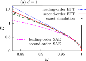
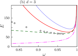
Figure 8: Oscillon energies $E(\omega)$ in the model (6) as predicted by two orders of the EFT (dotted and solid lines) and two orders of the small-amplitude expansion (SAE, dash-dotted and dashed lines). Theoretical predictions are compared with the results of exact numerical simulations (circles with errorbars). Figures (a) and (b) correspond to $d=1$ and $3$ dimensions, respectively.

It is worth reminding that the EFT is not equivalent to the small-amplitude approach even at ${\omega\approx 1}$. Indeed, these methods have different expansion parameters: $R^{-1}\to 0$ at finite $\varphi$ (EFT), and $R^{-1}\sim\varphi\to 0$ (small-amplitude). To compare the approximations, we solved Eqs. (67) in the model (6) and obtained the oscillon energies $E(\omega)$ in the first two orders of small-amplitude expansion. In Figs. 8a and 8b we compare these results (dash-dotted and dashed lines, respectively) with the leading-order and second-order EFT predictions (dotted and solid lines), as well as with the results of exact numerical simulations (circles with errorbars). We consider the cases of $d=1$ and $3$ dimensions. It is clear that the EFT works better in lower $d$ but becomes less precise than small-amplitude expansion in $d=3$. On the other hand, even in the leading order it predicts two — stable and unstable — branches of three-dimensional oscillons [cf. Eq. (41)], which is qualitatively correct. The small-amplitude expansion incorrectly suggests instability of all three-dimensional oscillons in the leading order, but becomes more precise in higher orders. We believe that these properties remain valid in other generic models.

9 Discussion

In this paper, we have developed a consistent Effective Field Theory (EFT) description of scalar oscillons with arbitrary amplitudes in the limit of large size. The main trick of the method is to perform a canonical transformation from the original field $\varphi$ and its momentum $\pi_{\varphi}=\partial_{t}\varphi$ to long-range variables $\psi(t,\,\boldsymbol{x})$ and $\psi^{*}(t,\,\boldsymbol{x})$. Once this is done, the effective classical action for smooth parts of $\psi$ and $\psi^{*}$ takes the form of a systematic gradient expansion with more spatial derivatives appearing in every next term. The sole parameter of the expansion is $(mR)^{-2}$, where $m$ is the field mass and $R$ is the spatial scale. At any order, such an effective theory has a global U(1) symmetry $\psi\to\psi\,\mathrm{e}^{-i\alpha}$ and, as a consequence, a family of nontopological solitons called oscillons. In the original, exact model, the $U(1)$ symmetry is broken by the nonperturbative to EFT effects — hence, the lifetimes of large-size oscillons are expected to be exponentially long in $(mR)^{2}$.

It is remarkable that all presently known long-lived oscillons have sizes $R$ exceeding the inverse field mass $m^{-1}$ by factors of few or even parametrically Fodor:2008es ; Amin:2010jq ; Olle:2019kbo ; Olle:2020qqy  — at least, we are not aware of notable exceptions from this rule. Thus, conservation of the U(1) charge Kasuya:2002zs ; Kawasaki:2015vga in the EFT may be universally responsible for the oscillon longevity. Importantly, the effective theory comes with conditions on the scalar potential $V(\varphi)$ needed for the existence of long-lived oscillons. We formulated them in terms of a fictitious mechanical motion $\varphi=\varphi(t)$ in the potential $V(\varphi)$ or, more specifically, in terms of the oscillation frequency $\Omega(I)$ as a function of the amplitude $I$ — the action variable in this mechanical system. Stationary solitons (oscillons) exist in the EFT only if $\Omega(I_{0})<m$ for some $I_{0}$, see Eqs. (32), and (33) for the complete list of conditions. Besides, the oscillons are large and hence long-living if the mechanical frequency is almost constant: $|\partial_{I}\Omega|\ll\Omega/I$ at $I\leq I_{0}$, cf. Eq. (37). In simple terms, these conditions mean that the potential $V(\varphi)$ is attractive and nearly quadratic, see also Olle:2020qqy ; Cyncynates:2021rtf . Finally, the oscillons are linearly stable with respect to long-range perturbations if the Vakhitov-Kolokolov criterion (41) is fulfilled.

We discussed two obvious ways to satisfy all requirements. First, the conditions are generically met in the small-amplitude limit $I\to 0$ if $V(\varphi)$ is attractive, see Eq. (39). This is the case when the standard nonrelativistic (small-amplitude) expansion Dashen:1975hd ; Kosevich1975 ; Fodor:2008es ; Fodor:2019ftc is applicable on par with the EFT. Second, the conditions are fulfilled if ${V=\tilde{\Omega}^{2}\,\varphi^{2}/2}$ and the function $\tilde{\Omega}(\varphi)$ is almost constant in the sense of Sec. 4.2. The latter option includes, in particular, monodromy potentials $V\propto\varphi^{n}$ with $n\approx 2$ which are known to support large-amplitude and exceptionally long-lived oscillons Olle:2019kbo ; Olle:2020qqy . It would be interesting to investigate such objects within the EFT.

The above two options do not exhaust all possibilities. In general, one may construct the appropriate function $\Omega(I)$ and then restore the potential $V(\varphi)$ using Eq. (38) (in the symmetric case). The resulting model should support long-lived oscillons. In particular, $\Omega(I)$ can be flatter in some range of $I$’s or have a minimum at some value. Then the evaporation rates of the respective oscillons should be non-monotonic in amplitude and frequency. Similar non-monotonic effects were numerically observed in Zhang:2020bec ; Olle:2020qqy ; Cyncynates:2021rtf , and some of them may correspond to features of $\Omega(I)$.

One may find calculation of the effective action technically compelling in models with nontrivial potentials. But in fact, this procedure can be automated using computer algebra. Namely, the transformation to $\psi$ and $\psi^{*}$ and all coefficients in the effective action can be computed symbolically in the form of long power-law series, which can be then summed up numerically. We discuss this possibility in Sec. 8. Using the same trick, one may try to apply the EFT to models with nontrivial field content, e.g. Zhang:2021xxa .

We performed extensive tests of the EFT. First, we demonstrated that the standard small-amplitude series for oscillons Fodor:2008es can be exactly reproduced by expanding the effective action in fields, see Sec. 8. Second, we compared the EFT predictions with the exact numerical simulations in the model with a plateau potential. Quite expectedly, the effective technique becomes precise in the case of large-size and long-lived objects. Besides, it works better in lower dimensions.

We believe that the classical EFT may have wider region of applicability than just field theoretical oscillons. In particular, it may be helpful for studying dynamical systems, see the toy example in Appendix B.

A fascinating project for the future is analytical calculation of the oscillon evaporation rates in the limit $R\to\infty$ for arbitrary field strengths. In Sec. 5 we numerically confirmed that these rates are exponentially small in the EFT expansion parameter $\eta\sim(mR)^{-1}\ll 1$. However, analytic derivation of the oscillon lifetimes is far beyond the scope of the present paper. Presumably, this can be done by extracting exponentially small, complementary to the EFT parts of the oscillon solutions via complex analysis, like in the case of small amplitudes Segur:1987mg ; Fodor:2008du ; Fodor:2009kf ; Fodor:2019ftc .

Yet another direction for future research is related to formal limit of zero spatial dimensions, $d\to 0$. Recall that spherically-symmetric field equation for $\varphi(t,\,r)$ remains nontrivial in $d=0$. In this paper we demonstrated that the respective “zero-dimensional” oscillons are exactly periodic and eternally living. This explains, why oscillating objects appear more frequently and live longer in lower dimensions Gleiser:2004an . One may try to approximate the lower-dimensional objects with zero-dimensional ones and then compute corrections in $d$.

Notably, our leading-order effective action becomes exact in $d=0$, since all higher-order terms in the derivative expansion are proportional to $d$. Accordingly, the EFT works better in lower dimensions.

Appendix A Numerical methods

We solve the spherically-symmetric equation for $\varphi(t,\,r)$ on a uniform radial lattice with ${N_{r}+1}$ sites ${r_{j}=j\Delta r}$ in a finite box ${0\leq r\leq L_{r}}$, ${\Delta r=L_{r}/N_{r}}$. The field values ${\varphi_{j}=\varphi(t,\,r_{j})}$ are stored on the lattice sites. In practice, $L_{r}=750$ and $375$ in $d\geq 1$ and ${d<1}$ dimensions, respectively. Besides, we use ${N_{r}=16384}$ sites in ${d<3}$, $N_{r}=32768$ in $d=3$, and repeat computations at twice smaller $N_{r}$ to control the discretization errors.

In the Hamiltonian form and in spherical symmetry, the field equation (5) reads,

$$\partial_{t}\varphi=\pi_{\varphi}\;,\qquad\partial_{t}\pi_{\varphi}=R[\varphi]\;,\qquad\mbox{where}\quad R\equiv\partial^{2}_{r}\varphi+\frac{d-1}{r}\,\partial_{r}\varphi-V^{\prime}(\varphi)\;.$$ (69)

We impose Neumann boundary conditions $\partial_{r}\varphi=0$ at the lattice boundaries $r=0$ and $L_{r}$. Discretization of spatial derivatives in Eq. (69) is done using fast Fourier transform (FFT). Namely, we Fourier-transform the field, ${\varphi(r)=\tilde{\varphi}_{0}+\sum_{k}\tilde{\varphi}_{k}\cos(p_{k}r)}$, where $\tilde{\varphi}_{k}$ is the image at discrete momenta ${p_{k}=\pi k/L_{r}}$, and compute the derivatives by acting with $\partial_{r}$ and $\partial_{r}^{2}$ on this representation. Say, the first derivative is given by the sum ${\partial_{r}\varphi(r_{j})=-\sum_{k}p_{k}\tilde{\varphi}_{k}\sin(p_{k}r_{j})}$ which is easily computed. In this way we get the right-hand side $R(r_{j})=R^{(j)}$ in Eqs. (69) with exponentially small accuracy ${\delta R^{(j)}\sim\exp(-\mbox{const}/\Delta r)}$: all numerical errors in the FFT procedure come from large momentum cutoff ${p_{k}<p_{\max}\equiv\pi/\Delta r}$ cropping exponentially small tails of Fourier images. In practice we exploit the FFTW3 library Frigo:2005zln .

We evolve Eq. (69) in time using fourth-order symplectic Runge-Kutta-Nyström (RKN4) integrator McLachlan:PDE ; Regan:Neuman . In this method every time step consists of four sequential replacements $\pi_{\varphi}\to\pi_{\varphi}+a_{\lambda}\,\Delta t\,R[\varphi]$, $\varphi\to\varphi+b_{\lambda}\,\Delta t\,\pi_{\varphi}$, where  $\lambda=1\dots 4$ and the parameters $a_{\lambda}$ and $b_{\lambda}$ are given in McLachlan:PDE ; Regan:Neuman ; in particular, $\sum a_{\lambda}=\sum b_{\lambda}=1$. Overall, this gives $O(\Delta t^{4})$ precision and exact conservation of a symplectic form. In calculations, we set ${\Delta t=10^{-2}}$ and use twice larger time step for numerical tests. All our parameters satisfy the stability criterion Regan:Neuman  ${\Delta t\lesssim 0.97\,\Delta r}$ of the RKN4 method.

Now, recall that we modify the field equation with the sponge $H(r)$ to absorb the outgoing radiation, see Eq. (44). The new term is incorporated into the RKN4 procedure by changing the $\pi_{\varphi}$ replacements to $\pi_{\varphi}\to(1+\frac{1}{2}a_{\lambda}H\Delta t)^{-1}\left\{(1-\frac{1}{2}a_{\lambda}H\Delta t)\,\pi_{\varphi}+a_{\lambda}\Delta tR[\varphi]\right\}$. We set ${H=0}$ at $r<R_{s}$ and $H=H_{0}\cdot(r-R_{s})^{2}$, $H_{0}=10^{-6}$ outside of this sphere. In ${d\geq 1}$ dimensions, we cover roughly one half of the lattice with the absorbing region: $R_{s}=400$. In ${d<1}$ the emitted linear waves grow at large $r$, so we move the sponge closer, ${R_{s}=50}$.

Finally, we obtain the energy $E$ and charge $N$ of oscillons discretizing the integrals (43), (17) in the second order. It is worth noting that in fractional $d$ the volume factors in the integrands have soft singularities $r^{d-1}$ which are explicitly accounted for. Also, we restrict all integrations to the regions $r<r_{\max}$ dominated by oscillons. Here $r_{\max}$ is the radius at which the energy and charge densities stop falling off exponentially.

The above algorithm remains stable even during long simulation runs up to ${t=2\cdot 10^{5}}$. We estimate the numerical errors by changing the lattice spacing $\Delta r$ and time step $\Delta t$. In this way, we checked that the discretization errors are exponentially sensitive to $\Delta r$ and proportional to $(\Delta t)^{4}$. The sizes of these two inaccuracies are roughly comparable. Typically, they are orders of magnitude below the relative level of $10^{-4}$ and reach this value in the worst case ${d=2}$, see Fig. 9. Finally, we checked energy conservation which is satisfied in $d\geq 1$ and $d=0$ with relative precision better than $10^{-9}$ and $5\cdot 10^{-5}$, respectively.

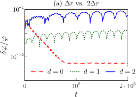
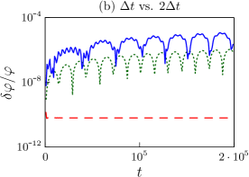
Figure 9: Maximal relative difference $\delta\varphi/\varphi\equiv\max_{r}|\delta\varphi|/\max_{r}|\varphi|$ between the two numerical solutions with ${\omega=0.99}$ which are computed (a) on grids with $N_{r}=16384$ and $8192$ i.e. at twice different $\Delta r$; (b) with time steps $\Delta t=10^{-2}$ and $2\cdot 10^{-2}$.

To end up, we remark that noticeable numerical errors in parameters $\omega$ and $E$ of oscillons come from the fact that these objects continuously radiate, lose energy and interfere with the emitted waves. To decrease the fluctuations, we averaged these parameters over ${P>1}$ consecutive oscillation periods and marked the sensitivity to $P$ with the errorbars in Figs. 5 and 8b. Numerical errors in all other figures are smaller than the circle size.

Appendix B A pedagogical example

Let us illustrate the classical EFT using two weakly coupled harmonic oscillators $\varphi_{1}(t)$ and $\varphi_{2}(t)$ with frequency $\Omega$ and Hamiltonian

$${\cal H}=\frac{1}{2}(\pi_{1}^{2}+\pi_{2}^{2})+\frac{\Omega^{2}}{2}(\varphi_{1}^{2}+\varphi_{2}^{2})+\frac{1}{2}\sum_{\alpha\beta}\lambda_{\alpha\beta}\;\varphi_{\alpha}\varphi_{\beta}\;.$$ (70)

Here $\pi_{\alpha}=\partial_{t}\varphi_{\alpha}$ are the canonical momenta and $\lambda_{\alpha\beta}\ll\Omega^{2}$ are small couplings. One can regard Eq. (70) as a crude discretization of the classical field with values $\varphi_{1}$, $\varphi_{2}$ at two spatial points and the last term in Eq. (70) representing gradient energy.

Explicit diagonalization of the Hamiltonian gives two eigenfrequencies,

$$\omega_{\pm}^{2}=\Omega^{2}+\frac{1}{2}\mathrm{tr}\,\lambda\pm\frac{1}{2}\sqrt{(\mathrm{tr}\,\lambda)^{2}-4\det\lambda}\;,$$ (71)

where $\mathrm{tr}\,\lambda$ and $\det\lambda$ are the trace and determinant of $\lambda_{\alpha\beta}$.

Let us derive this nontrivial formula using the classical EFT at $\lambda\ll\Omega^{2}$. In this case the oscillators $\varphi_{1}$ and $\varphi_{2}$ are almost independent, and the last term in Eq. (70) enables slow energy transfer between them. For a start, we introduce action-angle variables for every oscillator at $\lambda=0$,

$$\varphi_{\alpha}=\sqrt{\frac{2I_{\alpha}}{\Omega}}\,\cos\theta_{\alpha}\;,\qquad\pi_{\alpha}=-\sqrt{2I_{\alpha}\Omega}\,\sin\theta_{\alpha},\qquad h_{\alpha}\equiv(\pi_{\alpha}^{2}+\Omega^{2}\varphi_{\alpha}^{2})/2=\Omega I_{\alpha}\;.$$ (72)

Here $\alpha=1,\,2$ and $I_{\alpha}$ and $\theta_{\alpha}$ characterize oscillation amplitudes and phases, respectively. During the motion of decoupled oscillators $I_{\alpha}$ would be time-independent and ${\theta_{\alpha}=\Omega t+\mbox{const}}$.

Now, consider small nonzero $\lambda$. We perform canonical transformation (72) in the full Hamiltonian (70) and average its last (subdominant) term over the period of fast oscillations. It is convenient to introduce the quantities

$$\Theta=(\theta_{1}+\theta_{2})/2\qquad\mbox{and}\qquad\vartheta=(\theta_{1}-\theta_{2})/2\;.$$ (73)

In the decoupling limit $\lambda=0$, the value of $\Theta$ grows linearly in time and $\vartheta$ remains constant — these are the analogs of $\theta$ and $\partial_{i}\theta$ in field theory. Hence, we can average the subdominant term of the Hamiltonian over $\Theta$ instead of time, and move “slow” $\vartheta$ and $I_{\alpha}$ out of the averages, cf. Eq. (13). We obtain the effective Hamiltonian

$${\cal H}_{\mathrm{eff}}=\Omega(I_{1}+I_{2})+(\lambda_{11}I_{1}+\lambda_{22}I_{2})/(2\Omega)+\lambda_{12}\sqrt{I_{1}I_{2}}\,\cos(2\vartheta)/\Omega$$ (74)

describing long-time evolution of $I_{\alpha}$ and $\vartheta$. Notably, ${\cal H}_{\mathrm{eff}}$ is invariant under the global U(1) symmetry $\theta_{\alpha}\to\theta_{\alpha}+\gamma$ or $\Theta\to\Theta+\gamma$. This means that the respective Noether charge ${N=I_{1}+I_{2}}$ is conserved.

As a consequence of charge conservation, the effective theory has a set of stationary solutions with $\partial_{t}I_{\alpha}=\partial_{t}\vartheta=0$ and $\Theta=\omega t$. Indeed, one can check that this Ansatz passes the effective Hamiltonian equations. Such solutions are the eigenmodes with frequency $\omega$ in the mechanical system. Also, they are the direct analogs of oscillons in field theory.

Instead of solving the effective equations, we can extremize the energy at a fixed $N$, i.e., optimize the functional $F={\cal H}_{\mathrm{eff}}-\omega N$ with Lagrange multiplier $\omega$, cf. Eq. (24). Zero derivative with respect to $\vartheta$ is achieved at $\vartheta=0$ or $\pi/2$, while extremization over $I_{1}$ and $I_{2}$ gives,

$$2\Omega(\omega-\Omega)\sqrt{I_{1}}=\lambda_{11}\sqrt{I_{1}}\pm\lambda_{12}\sqrt{I_{2}}\!\quad\mbox{and}\quad\!\!\pm 2\Omega(\omega-\Omega)\sqrt{I_{2}}=\lambda_{12}\sqrt{I_{1}}\pm\lambda_{22}\sqrt{I_{2}}\,.$$ (75)

Here the upper and lower signs correspond to $\vartheta=0$ and $\pi/2$, respectively. Equations (75) mean that $\psi_{\alpha}=\{\sqrt{I_{1}},\;\pm\sqrt{I_{2}}\}$ is an eigenvector of the matrix $\lambda_{\alpha\beta}$ with an eigenvalue $2\Omega(\omega-\Omega)$. Solving this $2\times 2$ eigenvalue problem, we obtain,

$$\omega_{\pm}=\Omega+\frac{1}{4\Omega}\left[\mathrm{tr}\,\lambda\pm\sqrt{(\mathrm{tr}\,\lambda)^{2}-4\det\lambda}\right]\;,$$ (76)

where the $\pm$ signs discriminate between two eigenvalues; they are unrelated to those in Eq. (75). This result coincides with Eq. (71) up to corrections of order $(\omega-\Omega)^{2}=O(\lambda^{2})$. We conclude that the the EFT works at ${\lambda\ll\Omega^{2}}$. Once the stationary solutions are found, the Hamiltonian equation $\partial_{t}\Theta=\partial{\cal H}_{\mathrm{eff}}/\partial N=\omega$ tells us that $\Theta$ changes linearly in time, indeed.

Next, let us illustrate higher-order EFT corrections in the mechanical system (70). To this end we perform canonical transformation (72) in the full Hamiltonian. Besides, we break $I_{\alpha}$ and $\theta_{\alpha}$ into slow-varying and fast-oscillating parts:

$$I_{\alpha}=\bar{I}_{\alpha}+\delta I_{\alpha}\;,\qquad\qquad\theta_{\alpha}=\bar{\theta}_{\alpha}+\delta\theta_{\alpha}\;,$$ (77)

where $\langle\delta I_{\alpha}\rangle=\langle\delta\theta_{\alpha}\rangle=0$, ${\langle I_{\alpha}\rangle=\bar{I}_{\alpha}}$, and ${\langle\partial_{t}\theta_{\alpha}\rangle=\partial_{t}\bar{\theta}_{\alpha}}$. Equations for perturbations are obtained by writing down the exact Hamiltonian equations for $I_{\alpha}$ and $\theta_{\alpha}$ and subtracting their time averages. We obtain ${\partial_{t}\delta I_{\alpha}=j_{\theta,\,\alpha}}$ and ${\partial_{t}\delta\theta_{\alpha}=-j_{I,\,\alpha}}$, where

$$j_{\theta,\,\alpha}=-\sum\limits_{\beta}\lambda_{\alpha\beta}\left[\varphi_{\beta}\frac{\partial\varphi_{\alpha}}{\partial\theta_{\alpha}}-\Big{\langle}\varphi_{\beta}\frac{\partial\varphi_{\alpha}}{\partial\theta_{\alpha}}\Big{\rangle}\right],\;\;j_{I,\,\alpha}=-\sum\limits_{\beta}\lambda_{\alpha\beta}\left[\varphi_{\beta}\frac{\partial\varphi_{\alpha}}{\partial I_{\alpha}}-\Big{\langle}\varphi_{\beta}\frac{\partial\varphi_{\alpha}}{\partial I_{\alpha}}\Big{\rangle}\right]$$ (78)

are the sources, like in field theory, cf. Eqs. (50) and (51). Recall that the function $\varphi_{\alpha}(I_{\alpha},\,\theta_{\alpha})$ is given by Eq. (72) and note that $j_{I,\,\alpha}$, $j_{\theta,\,\alpha}\sim O(\lambda)$.

Now, we make the EFT approximations. First, we replace $I_{\alpha}$ and $\theta_{\alpha}$ in the sources with their leading-order parts $\bar{I}_{\alpha}$ and $\bar{\theta}_{\alpha}$. Second, we write the time derivative as $\partial_{t}\approx(\partial_{t}\bar{\Theta})\,\partial_{\bar{\Theta}}$, since $\bar{\Theta}=(\bar{\theta}_{1}+\bar{\theta}_{2})/2$ evolves almost linearly. This gives solutions for perturbations $\delta I_{\alpha}={\cal I}[j_{\theta,\,\alpha}]/\partial_{t}\bar{\Theta}$ and ${\delta\theta_{\alpha}=-{\cal I}[j_{I,\,\alpha}]/\partial_{t}\bar{\Theta}}$, where

$${\cal I}[f]=\int_{0}^{\bar{\Theta}}f(\bar{\Theta}^{\prime})\,d\bar{\Theta}^{\prime}-\Big{\langle}\int_{0}^{\bar{\Theta}}f(\bar{\Theta}^{\prime})\,d\bar{\Theta}^{\prime}\;\Big{\rangle}$$ (79)

is a primitive on the $\bar{\Theta}$ circle and $\langle\cdot\rangle$ now averages over this variable, cf. Eqs. (52) and (53). Explicitly,

$$\delta I_{\alpha}=-\sum_{\beta}\frac{\lambda_{\alpha\beta}\sqrt{\bar{I}_{\alpha}\bar{I}_{\beta}}}{2\Omega\,\partial_{t}\bar{\Theta}}\;\cos(\bar{\theta}_{\alpha}+\bar{\theta}_{\beta})\;,\qquad\delta\theta_{\alpha}=\sum_{\beta}\frac{\lambda_{\alpha\beta}\sqrt{\bar{I}_{\beta}}}{2\Omega\,\partial_{t}\bar{\Theta}\sqrt{\bar{I}_{\alpha}}}\;\sin(\bar{\theta}_{\alpha}+\bar{\theta}_{\beta})\;,$$ (80)

where we substituted Eq. (72) into Eqs. (78) and performed the $\bar{\Theta}$ integrals.

The last step of our method is to expand the full Hamiltonian in perturbations to the second order in $\lambda$, substitute the solutions (80) and average the resulting expression over $\bar{\Theta}$. We obtain $\mathcal{H}_{\text{eff}}=\mathcal{H}^{(1)}_{\text{eff}}+\mathcal{H}^{(2)}_{\text{eff}}$, where $\mathcal{H}^{(1)}_{\text{eff}}$ is given by Eq. (74) and the second-order correction is

$$\mathcal{H}^{(2)}_{\mathrm{eff}}=-\frac{2}{\partial_{t}\bar{\Theta}}\sum_{\alpha}\langle\,j_{I,\,\alpha}\,{\cal I}[j_{\theta,\,\alpha}]\,\rangle=-\sum_{\alpha\beta}\frac{(\lambda^{2})_{\alpha\beta}\sqrt{\bar{I}_{\alpha}\bar{I}_{\beta}}}{4\Omega^{2}\,\partial_{t}\bar{\Theta}}\;\cos(\bar{\theta}_{\alpha}-\bar{\theta}_{\beta})\;.$$ (81)

In the last equality $\lambda^{2}$ is a square of the matrix $\lambda$.

Note that in the main text we relied on the Lagrangian language, whereas this Appendix uses the Hamiltonian. This is equivalent: the second-order effective Lagrangian equals

$${\cal L}_{\mathrm{eff}}=\sum_{\alpha}(\,\bar{I}_{\alpha}\partial_{t}\bar{\theta}_{\alpha}\,)-{\cal H}_{\mathrm{eff}}^{(1)}-\frac{1}{2}{\cal H}_{\mathrm{eff}}^{(2)}+O(\lambda^{3})\;,$$ (82)

as one can see by performing the Legendre transform with respect to $\partial_{t}\bar{\theta}_{\alpha}$.

We test the second-order Hamiltonian by calculating the eigenfrequencies to the next order in $\lambda$. Note that ${\cal H}_{\mathrm{eff}}^{(1)}+{\cal H}_{\mathrm{eff}}^{(2)}$ is still invariant under the global symmetry $\bar{\Theta}\to\bar{\Theta}+\gamma$ because we averaged it over this variable. The respective global charge equals

$$N\equiv\sum_{\alpha}\frac{\partial{\cal L}_{\mathrm{eff}}}{\partial(\partial_{t}\bar{\theta}_{\alpha})}=\bar{I}_{1}+\bar{I}_{2}+\frac{\mathcal{H}^{(2)}_{\text{eff}}}{2\partial_{t}\bar{\Theta}}+O(\lambda^{3}).$$ (83)

As before, we find the eigenfrequencies by optimizing the functional ${F=\mathcal{H}_{\text{eff}}-\omega N}$. Extremum with respect to $\partial_{t}\bar{\Theta}$ and $\vartheta$ is achieved at $\partial_{t}\bar{\Theta}=\omega$ and $\vartheta=0$ or $\pi$. Varying over $\bar{I}_{1}$ and $\bar{I}_{2}$, we obtain the eigenvalue problem,

$$2\Omega(\omega-\Omega)\psi_{\alpha}=\sum_{\beta}\left(\lambda-\frac{\lambda^{2}}{4\omega\Omega}\right)_{\alpha\beta}\psi_{\beta}+O(\lambda^{3}\psi)\;,$$ (84)

where again $\psi_{\alpha}\equiv\{\sqrt{\bar{I}_{1}},\,\pm\sqrt{\bar{I}_{2}}\}$. We see that $\psi_{\alpha}$ is still an eigenvector of $\lambda$, but the eigenfrequency $\omega_{\pm}$ receives a correction

$$\omega_{\pm}^{(2)}=-\frac{1}{32\Omega^{3}}\left(\mathrm{tr}\,\lambda\pm\sqrt{(\mathrm{tr}\,\lambda)^{2}-4\det\lambda}\right)^{2}$$ (85)

that should be added to Eq. (75). Equation (85) is precisely the $O(\lambda^{2})$ term in the Taylor expansion of the exact eigenfrequency (71).

It is worth stressing that the EFT series in $\lambda$ converge, as is already clear from the exact result (71). This distinguishes our mechanical model from the field theory case: nonperturbative effects like the ones governing the decay of the field-theoretical oscillons do not appear. It could have been expected, since our system of harmonic oscillators admits exactly periodic motions.

Note also that although we performed mechanical calculations in the simplest illustrative model, classical EFT may be helpful for studying more involved dynamical systems. Indeed, this approach can be easily applied to essentially nonlinear models, e.g. to several weakly coupled anharmonic oscillators with slow dependencies of frequencies on amplitudes. Traditional treatment of the latter system relies on KAM theory Arnold which is not easy to use.

Appendix C One-dimensional oscillons

In one dimension, the mechanical equation (28) for the oscillon profile has a “conservation law,” i.e. $r$-independent quantity

$${\cal E}=\frac{1}{2}(\partial_{r}\chi)^{2}+U_{\omega}(\chi)=\frac{2\psi^{2}}{\mu_{I}}\,(\partial_{r}\psi)^{2}+\omega\psi^{2}-h\;,\qquad\qquad\partial_{r}{\cal E}=0\;,$$ (86)

where $r=|x|$ and we transformed back to $\psi(r)$ using Eqs. (26) and (27). Recall that the form factors $\mu_{I}$ and $h$ in Eq. (86) depend on $\psi^{2}$. We are interested in the localized solutions approaching $\psi\to 0$ as $r\to+\infty$. Hence, ${\cal E}=0$. Using Eq. (86), we immediately find,

$$r=\int_{\psi}^{\psi_{0}}\frac{\psi^{\prime}d\psi^{\prime}\sqrt{2}}{\sqrt{\mu_{I}(h-\omega\psi^{\prime 2})}}\;,$$ (87)

where the amplitude $\psi_{0}$ in the center satisfies equation $h(\psi_{0}^{2})/\psi_{0}^{2}=\omega$. In the model (6), we substitute $\mu_{I}$ and $h$ from Eqs. (18), (20) and obtain Eq. (34).

The main idea in calculating the charge $N$ and energy $E$ of one-dimensional oscillons is to change the integration variable in Eqs. (4) and (24) from $r$ to $\psi$ and then express $\partial_{r}\psi$ using Eq. (87). This gives,

$$N=2\int_{0}^{\infty}dr\,\psi^{2}(r)=2^{3/2}\int_{0}^{\psi_{0}}\frac{\psi^{3}d\psi}{\sqrt{\mu_{I}(h-\omega\psi^{2})}}$$ (88)

and similarly for $E$. Using the form factors in the model (6), we arrive at Eqs. (35), (36) from the main text.

Appendix D Vakhitov-Kolokolov criterion

In this Appendix we prove the Vakhitov-Kolokolov criterion (41) which, if broken, indicates instability of oscillons under small long-range perturbations. We will use the leading-order effective theory and energetic argument of vk ; Zakharov12 . The latter applies without essential modifications, and this is nontrivial, since EFT is an unusual theory with non-canonical gradient term for $\theta$ and nonlinear dependence of the charge $N$ on the second, canonically normalized field $\chi$, see Eqs. (14) and (27). Let us find out whether the oscillon solution $\chi=\chi(\boldsymbol{x})$ and $\theta=\omega t$ truly minimizes the energy $E$ at a fixed $N$, or it is just an unstable extremum. We add small perturbations $\delta\chi(\boldsymbol{x})$ and $\delta\theta(\boldsymbol{x})$ to the oscillon fields in such a way that $N$ in Eq. (4) remains unchanged:

$$\delta N=0\approx\int d^{d}\boldsymbol{x}\,\frac{dI}{d\chi}\,\delta\chi=(\nu|\delta\chi)\;,$$ (89)

where we omitted the higher-order terms in $\delta\chi$, introduced $\nu(\boldsymbol{x})=dI/d\chi=\sqrt{\mu_{I}}$ in accordance with Eq. (26), and defined the real scalar product ${(f|g)=\int d^{d}\boldsymbol{x}\,f(\boldsymbol{x})\,g(\boldsymbol{x})}$. Hereafter all coefficient functions, e.g. $\mu_{I}(\boldsymbol{x})\equiv\mu_{I}(\chi(\boldsymbol{x}))$, are evaluated on the background oscillon $\chi(\boldsymbol{x})$. Note that the norm of $\nu(\boldsymbol{x})$ is finite at finite charge $N$, since ${\nu^{2}=\mu_{I}\propto\psi^{2}(\boldsymbol{x})}$ in the weak-field region $|\boldsymbol{x}|\to+\infty$, see Eqs. (4) and (30).

At a fixed $N$, variations of energy and $F\equiv E-\omega N$ coincide. We obtain,

$$\delta E=\delta F\approx\frac{1}{2}(\delta\chi|\hat{L}_{\chi}|\delta\chi)+\frac{1}{2}(\delta\theta|\hat{L}_{\theta}|\delta\theta)\;,$$ (90)

where Eqs. (24), (26), and (27) were used, ${\hat{L}_{\chi}=-\Delta-U_{\omega}^{\prime\prime}(\chi(\boldsymbol{x}))}$ and ${\hat{L}_{\theta}=-\partial_{i}\,\mu_{\theta}^{-1}\,\partial_{i}}$ are the differential operators, and the primes denote $\chi$ derivatives. Recall that $\mu_{\theta}\geq 0$, and hence $\hat{L}_{\theta}$ is positive-definite, cf. Eq. (13). This means that the oscillons are stable if $\hat{L}_{\chi}$ is positive-definite in the subspace (89) of perturbations orthogonal to $\nu$.

It is remarkable that at least one eigenvalue of $\hat{L}_{\chi}$ is negative, and the only question is whether it survives projection onto the subspace (89). Indeed, taking the $r$ derivative of the profile equation (28), one gets $(\partial_{r}\chi|\hat{L}_{\chi}|\partial_{r}\chi)=-(d-1)(\partial_{r}\chi|r^{-2}|\partial_{r}\chi){<0}$ in ${d>1}$ dimensions. The same argument in $d=1$ implies that $\partial_{x}\chi(x)$ is a zero vector: $\hat{L}_{\chi}|\partial_{x}\chi)=0$. But this function also has a node, $\partial_{x}\chi=0$ at $x=0$, thus implying by the oscillation theorem that the eigenvector with smaller — negative — eigenvalue of $\hat{L}_{\chi}$ exists. We conclude that in any dimension $\hat{L}_{\chi}$ has a negative eigenvalue. In what follows we will use the orthonormal basis of $\hat{L}_{\chi}$ eigenvectors $\hat{L}_{\chi}|n)=w_{n}|n)$, where $w_{n}$ are the eigenvalues and ${w_{0}<0}$.

In the subspace (89) orthogonal to $|\nu)$ the eigenvalue problem for $\hat{L}_{\chi}$ has a different form:

$$\hat{L}_{\chi}|\delta\chi)-C|\nu)=w|\delta\chi)\;.$$ (91)

Here $w$ is the new eigenvalue and $C=(\nu|\hat{L}_{\chi}|\delta\chi)/(\nu|\nu)$ ensures that the left-hand side is orthogonal to $|\nu)$. Equation (91) can be solved in the full orthonormal basis of $\hat{L}_{\chi}$ eigenvectors: $|\delta\chi)=\sum_{n}\delta\chi_{n}|n)$ and $\delta\chi_{n}=C\,(n|\nu)/(w_{n}-w)$.

Once this is done, the eigenvalues $w$ in the subspace (89) are obtained by imposing condition $(\nu|\delta\chi)=0$. We find,

$$G(w)\equiv{\sum_{n}}^{\prime}(n|\nu)^{2}/(w_{n}-w)=0\;.$$ (92)

Note that $\hat{L}_{\chi}$ has zero modes $\partial_{i}\chi(\boldsymbol{x})$ representing shift symmetry: derivative of Eq. (28) gives ${\hat{L}_{\chi}|\partial_{i}\chi)=0}$. But they do not contribute into Eq. (92) because $(\partial_{i}\chi|\nu)=0$ as the integral of the full derivative. Besides, in generic case there are no other zero modes of $\hat{L}_{\chi}$. Thus, in Eq. (92) and below we sum over all $\hat{L}_{\chi}$ eigenmodes except for the ones with zero eigenvalues and equip the respective sums with primes.

By construction, the function $G(w)$ grows, $\partial_{w}G>0$, and has poles at the original $\hat{L}_{\chi}$ spectrum $w=w_{n}$. In particular, $G\to-\infty$ as $w$ approaches $w_{0}<0$ from the above. We conclude that the solution of Eq. (92) exists at $w<0$ if $G(0)>0$, i.e.,

$$0<G(0)={\sum_{n}}^{\prime}\,\frac{(\nu|n)(n|\nu)}{w_{n}}=(\nu|\hat{L}_{\chi}^{-1}|\nu)\;,$$ (93)

where the ambiguity of $\hat{L}_{\chi}^{-1}$ in the linear span of zero eigenvectors is removed by the matrix element with $|\nu)$. It is worth recalling that this condition guarantees negative eigenvalue $w<0$ for $\hat{L}_{\chi}$ in the subspace (89) and hence indicates instability of the background oscillon.

To simplify Eq. (93), we take a derivative of the profile equation (28) with respect to the oscillon frequency $\omega$. This gives ${\hat{L}_{\chi}\partial_{\omega}\chi=dI/d\chi=\nu(\boldsymbol{x})}$ or, inverting, $\hat{L}^{-1}_{\chi}|\nu)=|\partial_{\omega}\chi)$. Substituting this last equality into Eq. (93) and expressing the latter in terms of $dN/d\omega$, we get the opposite of Eq. (41), i.e. the condition for instability of oscillons.

Appendix E Second-order effective action

E.1 Generalities

In the EFT, we Taylor-expand Eq. (49) with respect to the perturbations $\delta I$ and $\delta\theta$ and average it over period. This strategy follows from the fact that the time integral in the action kills mixing between slow and fast quantities, e.g., $\int dt\,\bar{I}\,\partial_{t}\delta\theta\approx\int dt\,\bar{I}\langle\partial_{t}\delta\theta\rangle=0$. We will extensively use this simplification below. The term $\Phi\Delta\Phi$ is problematic, however, because $\Phi$ itself oscillates with $\bar{\theta}$. So, before expanding the Lagrangian we reorganize it: integrate by parts with respect to time, express $\partial_{t}\delta I$ and $\partial_{t}\delta\theta$ from the exact equations for perturbations (50), and then add and subtract the term $\Phi\Delta\bar{\Phi}/2$, where ${\bar{\Phi}\equiv\Phi(\bar{I},\,\bar{\theta})}$. This gives,

$${\cal S}=\int dtd^{d}{\boldsymbol{x}}\left[\bar{I}\partial_{t}\bar{\theta}+\frac{1}{2}\Phi\Delta\bar{\Phi}-h+\frac{1}{2}\Omega\delta I+\frac{\Delta\Phi}{2}\left(\Phi-\bar{\Phi}-\partial_{I}\Phi\,\delta I-\partial_{\theta}\Phi\,\delta\theta\right)\right]\,,$$ (94)

where all quantities without the overbar still depend on $I=\bar{I}+\delta I$ and $\theta=\bar{\theta}+\delta\theta$.

In the second-order EFT, we work to the quadratic order in $\delta I$ and $\delta\theta$. The bracket in the last term of Eq. (94) is already quadratic — hence, we can replace $\Delta\Phi$ in front of it with $\Delta\bar{\Phi}$. Expanding all terms, we obtain ${\cal S}\approx{\cal S}_{\mathrm{eff}}^{(1)}+{\cal S}^{(2)}_{\mathrm{eff}}$, where

$$\mathcal{S}_{\mathrm{eff}}^{(1)}=\int dtd^{d}\boldsymbol{x}\left[\bar{I}\partial_{t}\bar{\theta}-\bar{h}+\frac{1}{2}\bar{\Phi}\Delta\bar{\Phi}\right]\;,\qquad\mathcal{S}^{(2)}_{\mathrm{eff}}=\frac{1}{2}\int dtd^{d}\boldsymbol{x}\left[\Delta\bar{\Phi}\,\partial_{\bar{I}}\bar{\Phi}\,\delta I+\Delta\bar{\Phi}\,\partial_{\bar{\theta}}\bar{\Phi}\,\delta\theta\right].$$

The last step is to equip every term with the overall period average. This makes ${\cal S}_{\mathrm{eff}}^{(1)}$ coincide with the leading-order action (13), (14). The correction ${\cal S}_{\mathrm{eff}}^{(2)}$ takes the form (54) once the solutions for perturbations (52) and Eqs. (51) are substituted.

Now, we write down the second-order effective action in the case of oscillon: $\bar{\theta}=\omega t$ and ${\bar{I}=\bar{I}(\boldsymbol{x})}$. It is convenient to introduce short-hand notations

$$A(\bar{I},\bar{\theta}\,)=\mathcal{I}\left[\partial_{\bar{I}}\bar{\Phi}\,\partial_{\bar{\theta}}\bar{\Phi}\right]\;,\qquad\qquad B(\bar{I},\bar{\theta})=(\partial_{\bar{I}}\bar{\Phi})^{2}-\langle(\partial_{\bar{I}}\bar{\Phi})^{2}\rangle\;.$$ (95)

Some combinations of higher $\bar{\Phi}$ derivatives can be expressed via these quantities, e.g., ${\cal I}[\partial_{\bar{I}}^{2}\bar{\Phi}\,\partial_{\bar{\theta}}\bar{\Phi}]=\partial_{\bar{I}}A-B/2$, where the property ${\cal I}[\partial_{\bar{\theta}}f]=f-\langle f\rangle$ was used. In terms of $A$ and $B$ the sources (51) take the form,

$$j_{I}=B\,\Delta\bar{I}+\frac{1}{2}\partial_{\bar{I}}B\,(\partial_{i}\bar{I})^{2}\;,\qquad\mathcal{I}[j_{\theta}]=A\,\Delta\bar{I}+\frac{1}{2}(2\partial_{\bar{I}}A-B)(\partial_{i}\bar{I})^{2}\,.$$ (96)

Substituting these expressions into the action (54), we obtain the second-order correction $-F^{(2)}$ to the Lagrangian,

$$F^{(2)}=-\int d^{d}{\boldsymbol{x}}\left[c_{1}\,(\partial_{i}\bar{I})^{4}+c_{2}\,(\partial_{i}\bar{I})^{2}\Delta\bar{I}+c_{3}\,(\Delta\bar{I})^{2}\right]\;,$$ (97)

where the form factors $c_{i}$ depend on $\bar{I}$:

$$c_{1}=\frac{1}{4\omega}\,\big{\langle}\partial_{\bar{I}}B\,(2\partial_{\bar{I}}A-B)\big{\rangle}-\frac{\partial_{\bar{I}}\Omega}{8\omega^{2}}\,\big{\langle}(2\partial_{\bar{I}}A-B)^{2}\big{\rangle}\;,$$

$$c_{2}=\frac{1}{2\omega}\,\big{\langle}A\partial_{\bar{I}}B+2B\partial_{\bar{I}}A-B^{2}\big{\rangle}-\frac{\partial_{\bar{I}}\Omega}{2\omega^{2}}\,\langle 2A\partial_{\bar{I}}A-AB\rangle\;,$$ (98)

$$c_{3}=\frac{1}{\omega}\,\big{\langle}AB\big{\rangle}-\frac{\partial_{\bar{I}}\Omega}{2\omega^{2}}\,\langle A^{2}\rangle\;.$$

Notably, $c_{i}$ are quadratic in $A$ and $B$ and hence involve four $\bar{\Phi}$ multipliers in every term. We finally change variables to $\psi(\boldsymbol{x})=\sqrt{\bar{I}}$ and arrive to Eq. (56) with coefficients

$$d_{1}=16\psi^{4}c_{1}+8\psi^{2}c_{2}+4c_{3}\;,\qquad d_{2}=8(\psi^{2}c_{2}+c_{3})\;,\qquad d_{3}=4\psi^{2}c_{3}\;,$$ (99)

where the last formula coincides with Eq. (57) once $c_{3}$ and Eqs. (95) are substituted.

E.2 The model with a plateau potential

Next, we calculate the second-order EFT form factors $c_{i}$ and $d_{i}$ in the particular model (6). It will be convenient to use complex variable $z=-\exp(2i\bar{\theta})$ instead of $\bar{\theta}$; now, the period averages are given by the integrals over unit circle $|z|=1$, see Footnote 5. The function $\Phi(\bar{I},\,z)$ in Eq. (19) has singularities at $z=z_{1}$ and $z=z_{2}$,

$$z_{1}=2/\bar{I}-1\;,\qquad\qquad z_{2}=\bar{I}/(2-\bar{I})=z^{-1}_{1}\;,$$ (100)

which will appear in all expressions.

Substituting the expression (19) for $\Phi$ into Eqs. (95), we find $A=N_{A}\xi_{A}$ and ${B=N_{A}\xi_{B}}$, where we separated the $\bar{\theta}$ independent factor

$$N_{A}=\left[2\bar{I}(1-\bar{I})(2-\bar{I})\right]^{-1}$$ (101)

and denoted

$$\xi_{A}=\ln(1-z_{2}/z)+\ln(1-z/z_{1})\;,\qquad\xi_{B}=-\frac{2}{\bar{I}(2-\bar{I})}\left(\frac{z}{z_{1}-z}+\frac{z_{2}}{z-z_{2}}\right)\;.$$ (102)

It is remarkable that $\xi_{B}=\partial_{\bar{I}}\xi_{A}$. Using this property, we can express all period averages in the form factors (98) in terms of quantities $\langle\xi_{A}^{2}\rangle$ and $\langle(\partial_{\bar{I}}\xi_{A})^{2}\rangle$ and their $\bar{I}$ derivatives. Say, the third coefficient equals

$$c_{3}=\frac{N_{A}^{2}}{2\omega^{2}}\left(\omega\,\partial_{\bar{I}}\langle\xi_{A}^{2}\rangle+\langle\xi_{A}^{2}\rangle\right)\;,$$ (103)

and others have similar form; recall that $\Omega=1-\bar{I}$ in our model. Evaluating the contour integrals over $z$, we obtain,

$$\left\langle\xi^{2}_{A}\right\rangle=2\operatorname{Li}_{2}(z^{2}_{2})\qquad\text{and}\qquad\left\langle(\partial_{\bar{I}}\xi_{A})^{2}\right\rangle=\frac{2}{(1-\bar{I})(2-\bar{I})^{2}}\;,$$ (104)

where ${\mathrm{Li}_{2}(w)=-\int_{0}^{w}dw^{\prime}\,\ln(1-w^{\prime})/w^{\prime}}$ is the dilogarithm.

The final result is,

$$c_{1}=\; \frac{\ln(1-z_{2}^{2})\,\partial_{\bar{I}}N_{A}^{2}}{\omega\bar{I}(2-\bar{I})}\left\{\frac{2-2\bar{I}}{\bar{I}(2-\bar{I})}-\frac{1}{\omega}-\frac{\partial_{\bar{I}}N_{A}}{N_{A}}\right\}+\frac{(\partial_{\bar{I}}N_{A})^{2}}{\omega^{2}}\;\mathrm{Li}_{2}(z_{2}^{2})$$

$$\qquad\qquad\qquad\qquad+\frac{N_{A}^{2}}{4\omega(1-\bar{I})(2-\bar{I})^{2}}\,\left\{\frac{4-3\bar{I}}{(1-\bar{I})(2-\bar{I})}+6\,\frac{\partial_{\bar{I}}N_{A}}{N_{A}}+\frac{1}{\omega}\right\}\;,$$ (105)

$$c_{2}=\; \frac{2\ln(1-z_{2}^{2})\,N_{A}^{2}}{\omega\bar{I}(2-\bar{I})}\left\{\frac{2-2\bar{I}}{\bar{I}(2-\bar{I})}-\frac{3\partial_{\bar{I}}N_{A}}{N_{A}}-\frac{1}{\omega}\right\}+\frac{2N^{2}_{A}}{\omega(1-\bar{I})(2-\bar{I})^{2}}+\frac{\partial_{\bar{I}}N^{2}_{A}}{\omega^{2}}\;\mathrm{Li}_{2}(z^{2}_{2})\;,$$

$$c_{3}=\; \frac{N^{2}_{A}}{\omega}\left\{\frac{1}{\omega}\,\mathrm{Li}_{2}\left(z^{2}_{2}\right)-\frac{4\ln(1-z_{2}^{2})}{\bar{I}(2-\bar{I})}\right\}\;,$$

where $z_{2}$ and $N_{A}$ are given by Eqs. (100), (101). Now, $d_{i}$ can be found from Eqs. (99).

References

- (1) M. Gleiser, Pseudostable bubbles, Phys. Rev. D 49 (1994) 2978 [hep-ph/9308279].
- (2) A.E. Kudryavtsev, Solitonlike Solutions for a Higgs Scalar Field, JETP Lett. 22 (1975) 82.
- (3) I.L. Bogolyubsky and V.G. Makhankov, On the Pulsed Soliton Lifetime in Two Classical Relativistic Theory Models, JETP Lett. 24 (1976) 12.
- (4) E.W. Kolb and I.I. Tkachev, Axion miniclusters and Bose stars, Phys. Rev. Lett. 71 (1993) 3051 [hep-ph/9303313].
- (5) B. Piette and W.J. Zakrzewski, Metastable stationary solutions of the radial d-dimensional sine-Gordon model, Nonlinearity 11 (1998) 1103.
- (6) M. Gleiser and J. Thorarinson, A Class of Nonperturbative Configurations in Abelian-Higgs Models: Complexity from Dynamical Symmetry Breaking, Phys. Rev. D 79 (2009) 025016 [0808.0514].
- (7) M.A. Amin and D. Shirokoff, Flat-top oscillons in an expanding universe, Phys. Rev. D 81 (2010) 085045 [1002.3380].
- (8) M. Gleiser, N. Graham and N. Stamatopoulos, Long-Lived Time-Dependent Remnants During Cosmological Symmetry Breaking: From Inflation to the Electroweak Scale, Phys. Rev. D 82 (2010) 043517 [1004.4658].
- (9) P. Salmi and M. Hindmarsh, Radiation and Relaxation of Oscillons, Phys. Rev. D 85 (2012) 085033 [1201.1934].
- (10) M.A. Amin, K-oscillons: Oscillons with noncanonical kinetic terms, Phys. Rev. D 87 (2013) 123505 [1303.1102].
- (11) J. Sakstein and M. Trodden, Oscillons in Higher-Derivative Effective Field Theories, Phys. Rev. D 98 (2018) 123512 [1809.07724].
- (12) J. Ollé, O. Pujolàs and F. Rompineve, Oscillons and Dark Matter, JCAP 02 (2020) 006 [1906.06352].
- (13) H.-Y. Zhang, M. Jain and M.A. Amin, Polarized vector oscillons, Phys. Rev. D 105 (2022) 096037 [2111.08700].
- (14) H.-Y. Zhang, M.A. Amin, E.J. Copeland, P.M. Saffin and K.D. Lozanov, Classical Decay Rates of Oscillons, JCAP 07 (2020) 055 [2004.01202].
- (15) J. Olle, O. Pujolas and F. Rompineve, Recipes for oscillon longevity, JCAP 09 (2021) 015 [2012.13409].
- (16) E.W. Kolb and I.I. Tkachev, Nonlinear axion dynamics and formation of cosmological pseudosolitons, Phys. Rev. D 49 (1994) 5040 [astro-ph/9311037].
- (17) A. Vaquero, J. Redondo and J. Stadler, Early seeds of axion miniclusters, JCAP 04 (2019) 012 [1809.09241].
- (18) M. Buschmann, J.W. Foster and B.R. Safdi, Early-Universe Simulations of the Cosmological Axion, Phys. Rev. Lett. 124 (2020) 161103 [1906.00967].
- (19) M. Gorghetto, E. Hardy and G. Villadoro, More axions from strings, SciPost Phys. 10 (2021) 050 [2007.04990].
- (20) C.A.J. O’Hare, G. Pierobon, J. Redondo and Y.Y.Y. Wong, Simulations of axionlike particles in the postinflationary scenario, Phys. Rev. D 105 (2022) 055025 [2112.05117].
- (21) E.J. Copeland, M. Gleiser and H.R. Muller, Oscillons: Resonant configurations during bubble collapse, Phys. Rev. D 52 (1995) 1920 [hep-ph/9503217].
- (22) I. Dymnikova, L. Koziel, M. Khlopov and S. Rubin, Quasilumps from first order phase transitions, Grav. Cosmol. 6 (2000) 311 [hep-th/0010120].
- (23) E. Farhi, N. Graham, A.H. Guth, N. Iqbal, R.R. Rosales and N. Stamatopoulos, Emergence of Oscillons in an Expanding Background, Phys. Rev. D 77 (2008) 085019 [0712.3034].
- (24) J.R. Bond, J. Braden and L. Mersini-Houghton, Cosmic bubble and domain wall instabilities III: The role of oscillons in three-dimensional bubble collisions, JCAP 09 (2015) 004 [1505.02162].
- (25) M.A. Amin, R. Easther and H. Finkel, Inflaton Fragmentation and Oscillon Formation in Three Dimensions, JCAP 12 (2010) 001 [1009.2505].
- (26) M.A. Amin, R. Easther, H. Finkel, R. Flauger and M.P. Hertzberg, Oscillons After Inflation, Phys. Rev. Lett. 108 (2012) 241302 [1106.3335].
- (27) J.-P. Hong, M. Kawasaki and M. Yamazaki, Oscillons from Pure Natural Inflation, Phys. Rev. D 98 (2018) 043531 [1711.10496].
- (28) Y. Sang and Q.-G. Huang, Oscillons during Dirac-Born-Infeld preheating, Phys. Lett. B 823 (2021) 136781 [2012.14697].
- (29) D.G. Levkov, A.G. Panin and I.I. Tkachev, Gravitational Bose-Einstein condensation in the kinetic regime, Phys. Rev. Lett. 121 (2018) 151301 [1804.05857].
- (30) B. Eggemeier and J.C. Niemeyer, Formation and mass growth of axion stars in axion miniclusters, Phys. Rev. D 100 (2019) 063528 [1906.01348].
- (31) J. Chen, X. Du, E.W. Lentz, D.J.E. Marsh and J.C. Niemeyer, New insights into the formation and growth of boson stars in dark matter halos, Phys. Rev. D 104 (2021) 083022 [2011.01333].
- (32) J.H.-H. Chan, S. Sibiryakov and W. Xue, Condensation and Evaporation of Boson Stars, 2207.04057.
- (33) H.-Y. Schive, T. Chiueh and T. Broadhurst, Cosmic Structure as the Quantum Interference of a Coherent Dark Wave, Nature Phys. 10 (2014) 496 [1406.6586].
- (34) H.-Y. Schive, M.-H. Liao, T.-P. Woo, S.-K. Wong, T. Chiueh, T. Broadhurst et al., Understanding the Core-Halo Relation of Quantum Wave Dark Matter from 3D Simulations, Phys. Rev. Lett. 113 (2014) 261302 [1407.7762].
- (35) J. Veltmaat, J.C. Niemeyer and B. Schwabe, Formation and structure of ultralight bosonic dark matter halos, Phys. Rev. D 98 (2018) 043509 [1804.09647].
- (36) S.-Y. Zhou, E.J. Copeland, R. Easther, H. Finkel, Z.-G. Mou and P.M. Saffin, Gravitational Waves from Oscillon Preheating, JHEP 10 (2013) 026 [1304.6094].
- (37) J. Liu, Z.-K. Guo, R.-G. Cai and G. Shiu, Gravitational Waves from Oscillons with Cuspy Potentials, Phys. Rev. Lett. 120 (2018) 031301 [1707.09841].
- (38) K.D. Lozanov and M.A. Amin, Gravitational perturbations from oscillons and transients after inflation, Phys. Rev. D 99 (2019) 123504 [1902.06736].
- (39) Y. Sang and Q.-G. Huang, Stochastic Gravitational-Wave Background from Axion-Monodromy Oscillons in String Theory During Preheating, Phys. Rev. D 100 (2019) 063516 [1905.00371].
- (40) K.D. Lozanov and M.A. Amin, End of inflation, oscillons, and matter-antimatter asymmetry, Phys. Rev. D 90 (2014) 083528 [1408.1811].
- (41) H. Xiao, I. Williams and M. McQuinn, Simulations of axion minihalos, Phys. Rev. D 104 (2021) 023515 [2101.04177].
- (42) E. Cotner, A. Kusenko, M. Sasaki and V. Takhistov, Analytic Description of Primordial Black Hole Formation from Scalar Field Fragmentation, JCAP 10 (2019) 077 [1907.10613].
- (43) X.-X. Kou, C. Tian and S.-Y. Zhou, Oscillon Preheating in Full General Relativity, Class. Quant. Grav. 38 (2021) 045005 [1912.09658].
- (44) R. Garani, D. Levkov and P. Tinyakov, Solar mass black holes from neutron stars and bosonic dark matter, Phys. Rev. D 105 (2022) 063019 [2112.09716].
- (45) R.F. Dashen, B. Hasslacher and A. Neveu, The Particle Spectrum in Model Field Theories from Semiclassical Functional Integral Techniques, Phys. Rev. D 11 (1975) 3424.
- (46) A. Kosevich and A. Kovalev, Self-localization of vibrations in a one-dimensional anharmonic chain, JETP 40 (1975) 891.
- (47) G. Fodor, P. Forgacs, Z. Horvath and A. Lukacs, Small amplitude quasi-breathers and oscillons, Phys. Rev. D 78 (2008) 025003 [0802.3525].
- (48) G. Fodor, A review on radiation of oscillons and oscillatons, Ph.D. thesis, Wigner RCP, Budapest, 2019. 1911.03340.
- (49) H. Segur and M.D. Kruskal, Nonexistence of Small-Amplitude Breather Solutions in Theory, Phys. Rev. Lett. 58 (1987) 747.
- (50) G. Fodor, P. Forgacs, Z. Horvath and M. Mezei, Computation of the radiation amplitude of oscillons, Phys. Rev. D 79 (2009) 065002 [0812.1919].
- (51) G. Fodor, P. Forgacs, Z. Horvath and M. Mezei, Radiation of scalar oscillons in 2 and 3 dimensions, Phys. Lett. B 674 (2009) 319 [0903.0953].
- (52) E. Silverstein and A. Westphal, Monodromy in the CMB: Gravity Waves and String Inflation, Phys. Rev. D 78 (2008) 106003 [0803.3085].
- (53) L. McAllister, E. Silverstein and A. Westphal, Gravity Waves and Linear Inflation from Axion Monodromy, Phys. Rev. D 82 (2010) 046003 [0808.0706].
- (54) S. Kasuya, M. Kawasaki and F. Takahashi, I-balls, Phys. Lett. B 559 (2003) 99 [hep-ph/0209358].
- (55) M. Kawasaki, F. Takahashi and N. Takeda, Adiabatic Invariance of Oscillons/I-balls, Phys. Rev. D 92 (2015) 105024 [1508.01028].
- (56) R. Friedberg, T.D. Lee and A. Sirlin, A Class of Scalar-Field Soliton Solutions in Three Space Dimensions, Phys. Rev. D 13 (1976) 2739.
- (57) S.R. Coleman, Q-Balls, Nucl. Phys. B 262 (1985) 263.
- (58) E.Y. Nugaev and A.V. Shkerin, Review of Nontopological Solitons in Theories with -Symmetry, J. Exp. Theor. Phys. 130 (2020) 301 [1905.05146].
- (59) V.E. Zakharov and E.A. Kuznetsov, Solitons and collapses: two evolution scenarios of nonlinear wave systems, Phys. Usp. 55 (2012) 535.
- (60) M. Gleiser, d-dimensional oscillating scalar field lumps and the dimensionality of space, Phys. Lett. B 600 (2004) 126 [hep-th/0408221].
- (61) E. Braaten, A. Mohapatra and H. Zhang, Dense Axion Stars, Phys. Rev. Lett. 117 (2016) 121801 [1512.00108].
- (62) E. Braaten, A. Mohapatra and H. Zhang, Nonrelativistic Effective Field Theory for Axions, Phys. Rev. D 94 (2016) 076004 [1604.00669].
- (63) L. Visinelli, S. Baum, J. Redondo, K. Freese and F. Wilczek, Dilute and dense axion stars, Phys. Lett. B 777 (2018) 64 [1710.08910].
- (64) J. Eby, P. Suranyi, C. Vaz and L.C.R. Wijewardhana, Axion Stars in the Infrared Limit, JHEP 03 (2015) 080 [1412.3430].
- (65) K. Mukaida, M. Takimoto and M. Yamada, On Longevity of I-ball/Oscillon, JHEP 03 (2017) 122 [1612.07750].
- (66) J. Eby, K. Mukaida, M. Takimoto, L.C.R. Wijewardhana and M. Yamada, Classical nonrelativistic effective field theory and the role of gravitational interactions, Phys. Rev. D 99 (2019) 123503 [1807.09795].
- (67) B. Salehian, H.-Y. Zhang, M.A. Amin, D.I. Kaiser and M.H. Namjoo, Beyond Schrödinger-Poisson: nonrelativistic effective field theory for scalar dark matter, JHEP 09 (2021) 050 [2104.10128].
- (68) N.G. Vakhitov and A.A. Kolokolov, Stationary solutions of the wave equation in a medium with nonlinearity saturation, Radiophys. Quantum Electron. 16 (1973) 783.
- (69) R. Kallosh and A. Linde, Universality Class in Conformal Inflation, JCAP 07 (2013) 002 [1306.5220].
- (70) M. Gleiser and A. Sornborger, Longlived localized field configurations in small lattices: Application to oscillons, Phys. Rev. E 62 (2000) 1368 [patt-sol/9909002].
- (71) https://www.youtube.com/playlist?list=PLMxQF3HFStX3vjP4C7phmVMmjRgIFU7RV, 2022.
- (72) D. Cyncynates and T. Giurgica-Tiron, Structure of the oscillon: The dynamics of attractive self-interaction, Phys. Rev. D 103 (2021) 116011 [2104.02069].
- (73) L.D. Landau and E.M. Lifshitz, Course of Theoretical Physics. Volume 1. Mechanics, Butterworth-Heinemann (1976).
- (74) V. Arnold, Mathematical Methods of Classical Mechanics, Springer-Verlag (1989).
- (75) A.B. Adib, M. Gleiser and C.A.S. Almeida, Long lived oscillons from asymmetric bubbles: Existence and stability, Phys. Rev. D 66 (2002) 085011 [hep-th/0203072].
- (76) A.S. Dmitriev, D.G. Levkov, A.G. Panin, E.K. Pushnaya and I.I. Tkachev, Instability of rotating Bose stars, Phys. Rev. D 104 (2021) 023504 [2104.00962].
- (77) I.I. Tkachev, An Axionic Laser in the Center of a Galaxy?, Phys. Lett. B 191 (1987) 41.
- (78) D.G. Levkov, A.G. Panin and I.I. Tkachev, Radio-emission of axion stars, Phys. Rev. D 102 (2020) 023501 [2004.05179].
- (79) E.P. Honda and M.W. Choptuik, Fine structure of oscillons in the spherically symmetric phi**4 Klein-Gordon model, Phys. Rev. D 65 (2002) 084037 [hep-ph/0110065].
- (80) M. Frigo and S.G. Johnson, The Design and Implementation of FFTW3, IEEE Proc. 93 (2005) 216.
- (81) R.I. McLachlan, Expilicit Symplectic Splitting Methods Applied to PDEs, Lectures in Applied Mathematics 29 (1993) 325.
- (82) H.M. Regan, Von Neumann Stability Analysis of Symplectic Integrators Applied to Hamiltonian PDEs, Journal of Computational Mathematics 20 (2002) 611.