A 2D Model for Coronal Bright Points:
Association with Spicules, UV bursts, Surges and EUV Coronal Jets

Abstract

Coronal Bright Points (CBPs) are ubiquitous structures in the solar atmosphere composed of hot small-scale loops observed in EUV or X-Rays in the quiet Sun and coronal holes. They are key elements to understand the heating of the corona; nonetheless, basic questions regarding their heating mechanisms, the chromosphere underneath, or the effects of flux emergence in these structures remain open. We have used the Bifrost code to carry out a 2D experiment in which a coronal-hole magnetic nullpoint configuration evolves perturbed by realistic granulation. To compare with observations, synthetic SDO/AIA, Solar Orbiter EUI-HRI, and IRIS images have been computed. The experiment shows the self-consistent creation of a CBP through the action of the stochastic granular motions alone, mediated by magnetic reconnection in the corona. The reconnection is intermittent and oscillatory, and it leads to coronal and transition-region temperature loops that are identifiable in our EUV/UV observables. During the CBP lifetime, convergence and cancellation at the surface of its underlying opposite polarities takes place. The chromosphere below the CBP shows a number of peculiar features concerning its density and the spicules in it. The final stage of the CBP is eruptive: magnetic flux emergence at the granular scale disrupts the CBP topology, leading to different ejections, such as UV bursts, surges, and EUV coronal jets. Apart from explaining observed CBP features, our results pave the way for further studies combining simulations and coordinated observations in different atmospheric layers.

1 INTRODUCTION

Coronal Bright Points (CBPs) are a fundamental building block in the solar atmosphere. Scattered over the whole disc, CBPs consist of sets of coronal loops linking opposite polarity magnetic patches in regions of, typically, from $4$ to $43$ Mm transverse size, with heights ranging from $5$ to $10$ Mm (see the review by Madjarska, 2019). One of their most striking features is the sustained emission, for periods of several hours up to a few days, of large amounts of energy, which lend them their enhanced extreme-ultraviolet (EUV) and X-ray signatures (e.g., Golub et al., 1974).

A significant fraction of the CBPs are observationally found to be formed as a consequence of chance encounters of opposite magnetic polarities at the surface (e.g., Harvey, 1985; Webb et al., 1993; Mou et al., 2018). First theoretical explanations about this mechanism came in the 1990’s through analytical models under the name of Converging Flux Models (Priest et al., 1994; Parnell & Priest, 1995). There, the approaching motion in the photosphere of two opposite polarities that are surmounted by a nullpoint leads to reconnection and heating of coronal loops. Since then, this idea has been extended and studied using magnetohydrodynamics (MHD) experiments (e.g., Dreher et al., 1997; Longcope, 1998; Galsgaard et al., 2000; von Rekowski et al., 2006; Santos & Büchner, 2007; Javadi et al., 2011; Wyper et al., 2018; Priest et al., 2018; Syntelis et al., 2019). However, the available CBP models are idealized, i.e., they rely on ad-hoc driving mechanisms, which do not reflect the stochastic granular motions, they lack radiation transfer to model the lower layers of the atmosphere, and/or miss optically thin losses and/or thermal conduction to properly capture the CBP thermodynamics.

To understand the physics of CBPs, realistic numerical experiments are needed to address important open questions such as (a) the CBP energization, focusing on whether the granulation is enough to drive and sustain the reconnection at coronal heights to explain the CBP lifetimes; (b) the role of magnetic flux emergence, specially at the granular scale, to know whether it can disrupt the CBP topology and originate an eruption; and (c) the chromosphere underneath a CBP, with the aim of unraveling the unexplored impact of CBPs on the spicular activity and vice-versa.

In this letter, we model a CBP through the evolution of an initial fan-spine nullpoint configuration. The choice of this configuration is because CBPs often appear above photospheric regions with a parasitic magnetic polarity embedded in a network predominantly of the opposite polarity, which typically leads to a nullpoint structure in the corona (Zhang et al., 2012; Galsgaard et al., 2017; Madjarska et al., 2021). The 2D experiment is carried out with the Bifrost code (Gudiksen et al., 2011), which self-consistently couples the different layers of the solar atmosphere and incorporates several physical mechanisms not included in CBP modeling in the past. To provide a direct link to observations, we calculate synthetic EUV images for SDO/AIA (Pesnell et al., 2012; Lemen et al., 2012), and Solar Orbiter (SO)/EUI-HRI (Müller et al., 2020; Rochus et al., 2020), and UV images for IRIS (De Pontieu et al., 2014).

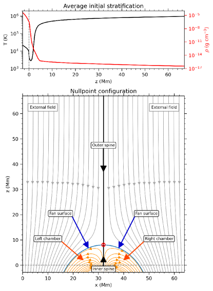
Figure 1: Initial condition. Top: Average stratification for the temperature and density. Bottom: Imposed magnetic field configuration indicating some of its major features following the terminology used in 3D nullpoints (Priest & Titov, 1996). Red circle: region with $B<1$ G centered on the nullpoint, $(x_{0},z_{0})=(32,8)$ Mm. Grey-dashed line: solar surface at $z=0$.

2 METHODS

2.1 Code

The experiment has been performed using Bifrost, a radiation-MHD code for stellar atmosphere simulations (Gudiksen et al., 2011). The code includes radiative transfer from the photosphere to the corona; the main losses in the chromosphere by neutral hydrogen, singly-ionized calcium and magnesium; thermal conduction along the magnetic field lines; optically thin cooling; and an equation of state with the 16 most important atomic elements in the Sun.

2.2 Initial Condition

2.2.1 Background Stratification

The initial condition has been constructed using as background a preexisting 2D numerical simulation with statistically stationary convection in the photosphere and below. It encompasses from the uppermost layers of the solar interior to the corona ($-2.8$ Mm $\leq z\leq 67.0$ Mm, $z=0$ being the solar surface). The horizontal extent is $0.0$ Mm $\leq x\leq 64.0$ Mm. The grid is uniform with $4096\times 4096$ cells, yielding a very high spatial resolution of $\Delta x=15.6$ km and $\Delta z=17.0$ km. The boundary conditions are the same as for the experiment by Nóbrega-Siverio et al. (2016). The top panel of Figure 1 shows the horizontal averages of temperature and density of the background stratification.

2.2.2 Nullpoint Configuration

Over the previous snapshot, we have imposed a potential magnetic nullpoint configuration as shown in the bottom panel of Figure 1. The potential field was calculated from a prescribed distribution at the bottom boundary, $z=-2.8$ Mm. The nullpoint is located at $(x_{0},z_{0})=(32,8)$ Mm and the field asymptotically becomes vertical in height with $B_{z}=-10$ G, mimicking a coronal hole structure. The photospheric field contains a positive parasitic polarity at the center on a negative background. At $z=0$, the total positive flux and maximum vertical field strength are $\Phi^{+}=2.2\times 10^{10}$ G cm and $B_{z}=41.3$ G, respectively; the parasitic polarity covers 9.7 Mm; and the fan surface extends for 28.1 Mm. We will refer to the closed-loop domains on either side of the inner spine as chambers.

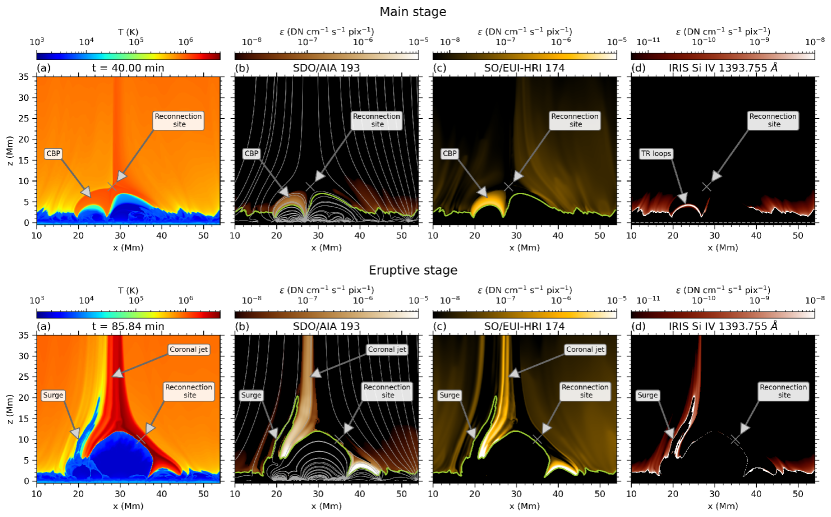
Figure 2: Experiment overview. Top: Main stage illustrating a CBP at $t=40.00$ min. Bottom: Eruptive stage showing a surge and coronal jet at $t=85.84$ min. (a) Temperature. (b) Synthetic SDO/AIA 193 with superimposed magnetic field lines. (c) SO/EUI-HRI 174. (d) IRIS Si IV 1393.755 Å. For the synthesis details, check Appendix A. Olive line on Panels (b) and (c): $T=10^{5}$ K isocontour. The associated movie comprises the whole experiment evolution from $t=0$ to $t=85.84$ min, illustrating the development of both stages.
(An animation of this figure is available.)

3 RESULTS

3.1 Overview of the Experiment

Figure 2 and associated movie provide an overview of the system evolution using temperature maps and synthetic observables for coronal and transition region (TR) temperatures (see Appendix A). In the experiment, the granulation quickly distorts the imposed magnetic field and reconnection is triggered as a consequence of perturbations at the nullpoint. We distinguish two well-defined phases: main stage and eruptive stage, summarized in the following and described in Sections 3.2 and 3.3, respectively.

The main stage (from $t=0$ to $t\approx 65$ min) covers the appearance of post-reconnection hot loops that leads to a CBP. For instance, at $t=40$ min (top row of Figure 2), our CBP is discernible as a set of hot coronal loops with enhanced SDO/AIA 193 and SO/EUI-HRI 174 emission above TR temperature loops visible in IRIS Si IV. This matches the SDO/IRIS observations by Kayshap & Dwivedi (2017), where CBPs are inferred to be composed of hot loops overlying cooler smaller ones. Our CBP is found in the left chamber, indicating that there is a preferred reconnection direction, and it gets more compact with time before vanishing, as reported in observations Mou et al. (2018).

In the eruptive stage, the CBP comes to an end. Around $t=67$ min in the animation, a first hot ejection results from reconnection between emerging plasma at granular scale and the magnetic field of the right chamber, resembling the UV burst described by Hansteen et al. (2019). More episodes of flux emergence and reconnection take place subsequently, dramatically destabilizing the system and producing more ejections. As an example, at $t=85.84$ min (bottom row of Figure 2) a large and broad hot coronal jet is seen next to a cool surge, reminiscent of previous results by Yokoyama & Shibata (1996); Moreno-Insertis & Galsgaard (2013); Nóbrega-Siverio et al. (2016). The synthesis clearly reflects the high spatial resolution of SO/EUI-HRI to study coronal jets and shows that the surroundings of the surge have significant Si IV emission, similarly to observations (e.g., Nóbrega-Siverio et al., 2017; Guglielmino et al., 2019).

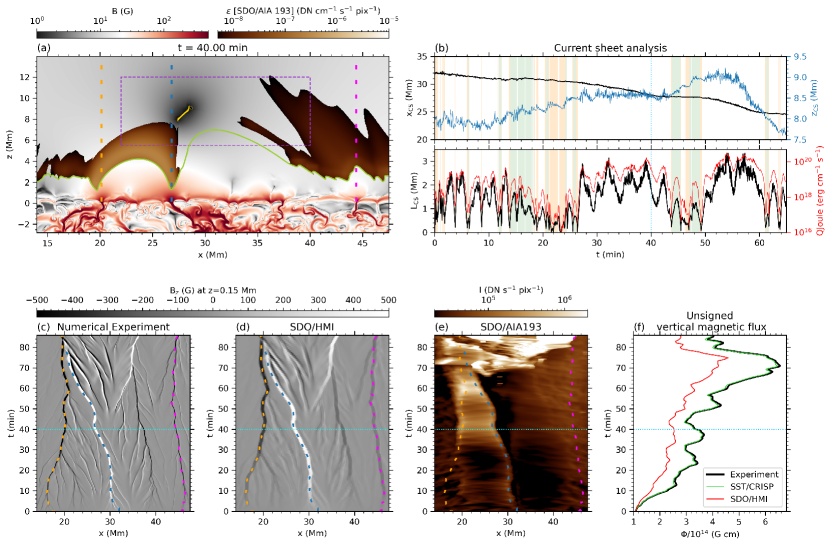
Figure 3: Magnetic reconnection and flux emergence. (a) $B$ at $t=40.00$ min with superimposed AIA 193 response only for the values contained in the corresponding color scale. Olive line: $T=10^{5}$ K isocontour. Purple rectangle: region for the current sheet (CS) analysis. Yellow dots: CS region given by $L_{B}\leq 100$ km, as defined in Appendix B. (b) CS analysis. Top: CS center coordinates, $x_{\mathrm{CS}}$ and $z_{\mathrm{CS}}$. Bottom: CS length, $L_{\mathrm{CS}}$, and Joule heating, $Q_{\mathrm{Joule}}$. When the CS is elongated, positive/negative angles of reconnection are indicated with white/green areas; otherwise, using orange. (c) Space-time map for $B_{z}$ at $z=0.15$ Mm. (d) View of (c) with the HMI resolution. (e) AIA 193 intensity integrated along the vertical direction. (f) Unsigned vertical magnetic flux for the experiment and corresponding ones for SST/CRISP and HMI resolutions measured at $z=0.15$ Mm. In the figure, colored dashed lines follow the polarities related to the left side of the fan surface (orange), the inner spine (blue), and the right side of the fan surface (magenta). The cyan-dotted lines indicates the time shown in Panel (a). The associated movie shows the evolution of the magnetic field and SDO/AIA 193 response from $t=0$ to $t=85.84$ min.
(An animation of this figure is available.)

3.2 Main Stage

3.2.1 Magnetic Reconnection and Association with CBP Features

To illustrate the crucial role of coronal reconnection for the CBP during the main stage, Panel (a) of Figure 3 contains the magnetic field strength with the SDO/AIA 193 response superimposed. Soon after starting the experiment (see animation), a current sheet (CS) is formed (yellow dots in the panel). Focusing on the region delimited by the purple rectangle, we distinguish three clear patterns: (a) the reconnection site slowly drifts to the left; (b) the reconnection and associated heating behaves in a bursty way; and (c) the reconnection is oscillatory.

The reconnection-site’s displacement is shown in the top frame of Panel (b). The horizontal position of the CS center, $x_{\mathrm{CS}}$ (black), moves 7.4 Mm to the left in 65 minutes, while its vertical position, $z_{\mathrm{CS}}$ (blue), first moves from 8.0 Mm up to 9.2 Mm, to descend later to 7.6 Mm. These results are akin to observations, where CBP nullpoints are inferred to rise, descend, or show both types of behavior in addition to important horizontal displacement (Galsgaard et al., 2017).

The bursty behavior is depicted in the bottom frame of Panel (b). The CS length, $L_{\mathrm{CS}}$, abruptly changes over times of minutes, reaching a maximum of $3.3$ Mm. These fluctuations are well correlated with the Joule heating released in the reconnection site, $Q_{\mathrm{Joule}}$: the Pearson correlation coefficient between both curves is 0.93. Note that when the diffusion region does not have an elongated CS (orange background in the panel), the Joule heating is minimal. This intermittent heating seems to be consistent with observed CBP emission variations over timescales of minutes (see, e.g, Habbal & Withbroe, 1981; Ugarte-Urra et al., 2004; Kumar et al., 2011; Ning & Guo, 2014; Chandrashekhar & Sarkar, 2015; Gao et al., 2022).

The elongated CS also changes its angle, $\theta_{\mathrm{CS}}$ (defined anticlockwise with respect to the x-axis), several times, from, approximately, $45$ to $-45$ degrees, indicating oscillatory reconnection. Panel (b) shows a white/green background for the intervals when $\theta_{\mathrm{CS}}$ is positive/negative. Most of the time, the angle is positive: the reconnection inflows come from the right chamber and the upper-left part of the external field, while the outflows are located in the left chamber and upper-right part of the external field. This explains why the left chamber is the one showing the CBP, as hot post-reconnection loops are being deposited predominantly in this region. The predominance seems to be associated with the concentration near the inner spine of the structure, indicated with a blue-dashed line in Panel (a), which mainly moves to the left (see animation). Oscillatory reconnection is also found in CBP observations (Zhang et al., 2014).

3.2.2 The Photospheric Magnetic Field

Figure 3 contains space-time magnetograms near the photosphere ($z=0.15$ Mm) with the actual resolution of the simulation (Panel (c)) and reducing it to the level of the SDO/HMI instrument (Panel (d), see Appendix A). To emphasize the CBP evolution, Panel (e) contains a space-time diagram showing the synthesized intensity of SDO/AIA 193 integrated along the vertical line-of-sight. Panels (a), (c) and (d) show that the magnetic field around the photospheric basis is quickly concentrated by the granular motions, leading to strong magnetic patches at the solar surface. In the figure, we have highlighted with colored dashed lines the concentrations that have collected the field lines near the fan surface on each side (orange and magenta) and near the inner spine (blue). The magnetic field concentrations are buffeted and dragged by the granular motions while being substantially deformed in the convection zone. In fact, the one related to the inner spine gets bent several times underneath the surface and develops horizontal magnetized structures (see animation of Panel (a) from $t\approx 20$ to $30$  min at $z\approx-1$ Mm and $x$ between 30 and 32 Mm). Simultaneously with the convergence at the photosphere of the two strong opposite concentrations (orange and blue lines), the post-reconnection loops in the corona start to brighten up in the EUV bands (see the superimposed SDO/AIA 193 response in Panel (a) and the space-time diagram of Panel (e)) marking the appearance of our CBP at around $t=30$ min. From observations, convergence is frequently involved in CBP formation (see, e.g., Mou et al., 2016, 2018, and references therein). The convergence continues, and the CBP goes through a quiet phase until around $t=65$ min, when the eruptive phase starts, triggered by flux emergence, as explained in the next section.

3.3 Eruptive Stage

3.3.1 Magnetic Flux Emergence at the Surface

The strong and complex subphotospheric magnetic structures developing around the inner spine mentioned in the previous section become buoyant and rise. They reach the surface to the right of the inner spine from $t=42$ min onwards, leading to anomalous granulation and increasing the unsigned vertical magnetic flux. The enhanced magnetic pressure in the anomalous granules further pushes the strong positive patch to the left, accelerating the convergence of the two main opposite polarities of the CBP. Panel (f) shows the total unsigned flux in the horizontal domain of Figure 3, i.e.,

$$\Phi=\int_{x_{0}=14.0\,\mathrm{Mm}}^{x_{f}=47.5\,\mathrm{Mm}}{\left|B_{z}(z=0)\right|dx},$$ (1)

with the integral calculated with the $B_{z}$ distributions in the experiment (black curve) and in the reduced-resolution counterparts for SST/CRISP (green) and SDO/HMI (red). The unsigned flux grows roughly by a factor two from $t=42$ min to $t=70.67$ min, when it reaches its maximum. Interestingly, in contrast to a high-resolution instrument like SST/CRISP, the reduced resolution of SDO/HMI would miss a significant fraction of the flux. From this time onwards, the unsigned magnetic flux at the surface decreases while the two main polarities continue converging. This could be interpreted as magnetic cancellation, a fact that is frequently observed at the end of CBPs (e.g., Mou et al., 2016, 2018).

Figure 4: Chromospheric analysis. Left: Space-time maps for $z^{max}_{10^{4}\hskip 0.3pt\mathrm{K}}(x)$. Right: Corresponding density $\rho(x,z^{max}_{10^{4}\hskip 0.3pt\mathrm{K}})$. Dashed lines: CBP’s main polarities (see also Figure 3). Red-solid lines: fan surface at $z=1.5$ Mm in the main stage.

3.3.2 Eruptive ejections

In the atmosphere, the emerging field quickly expands, interacting with the preexisting magnetic structure of the right chamber and leading to eruptive behavior with different ejections. The first one occurs at $t=67$ min, between $x=24$ and 30 Mm, and it resembles a UV burst because of its enhanced TR emission (see animation of Figure 2). The evolution of the system becomes quite complex at this stage. The current sheet of the UV burst interacts with the CBP current sheet, disrupting its magnetic configuration and causing the end of our CBP (see the horizontal dark band at $t=71$ min in Panel (d) of Figure 3). Another ejection with EUV signatures occurs right after, around $t=74$ min, developing an Eiffel tower shape, followed by the ejection of the broad EUV jet (reaching up to 13 MK) and surge that are shown in the bottom row of Figure 2.

3.4 The Chromosphere and Spicular Activity

To analyze the chromosphere below the CBP, Figure 4 illustrates space-time maps for $z^{max}_{10^{4}\hskip 0.3pt\mathrm{K}}(x)$, defined as the maximum height at which $T=10^{4}$ K for each $x$, and the corresponding density $\rho(x,z^{max}_{10^{4}\hskip 0.3pt\mathrm{K}})$ at that point. A major distinction is apparent between the regions inside and outside the fan surface. To clearly separate them, red-solid lines have been drawn at the horizontal position where the fan surface cuts the plane $z=1.5$ Mm. Those outside have an interesting flake or scale-like appearance. Each scale is flanked by a quasi-parabolic trajectory signaling the rise and fall of individual spicules: an example is indicated around $x=5$ Mm and $t\approx$ 44 min.

During the main stage, mainly from $t=30$ to $t=65$ min, the strong field in the CBP’s opposite polarities (dashed tracks) lowers the height of the chromospheric level below $2$ Mm. As these polarities converge, the chromosphere underneath the CBP (i.e., in the left chamber) gradually moves down, from $4$ Mm to 1 Mm, while the density roughly increases by an order of magnitude there. This region also shows some spicules, predominantly originated near the fan surface, with associated propagating disturbances that cross the magnetic field loops of this region (see example of both phenomena indicated within the left chamber).

The most striking characteristic of the right chamber is the enormous rarefaction during the main stage resulting from the predominant reconnection direction that extracts plasma from here (a fact also found in idealized 3D nullpoint simulations without flux emergence by Moreno-Insertis and Galsgaard, in preparation). In fact, the density can be so low as a few $10^{-17}$ g cm^-3: these are coronal densities with cold temperatures. There are also spicular incursions in this chamber mainly coming from regions around the fan surface (see example around $x=39$ Mm and $t=$ 32 min), but without associated propagating disturbances. In the eruptive stage, the leftmost part of the domain with $z^{max}_{10^{4}\hskip 0.3pt\mathrm{K}}(x)>8$ Mm corresponds to the ejection of the surge. Trajectories of multiple dense plasmoids expelled from the reconnection site are also visible with a fibril-like pattern.

4 DISCUSSION

In this letter we have shown that a wide class of CBPs may be obtained through magnetic reconnection in the corona driven by stochastic granular motions. Our numerical experiment has significant differences to previous CBP models: in contrast to, e.g., Priest et al. (1994, 2018) or Syntelis et al. (2019); Syntelis & Priest (2020), the magnetic field topology consists in a nullpoint created by a parasitic polarity within a coronal hole environment; more importantly, the reconnection and creation of the CBP is self-consistently triggered by the convection that naturally occurs in the realistic framework provided by the Bifrost code. The latter feature also sets it apart from the idealized CBP coronal hole model of Wyper et al. (2018), in a which high-velocity horizontal driving at the photosphere is imposed to provide the energy released in the CBP.

Our experiment shows striking similarities to observed CBP features in spite of the simplified 2D configuration. For instance, the CBP is composed of loops at different temperatures, with hotter loops overlying cooler smaller ones, and enhanced EUV/UV emission akin to observations (Kayshap & Dwivedi, 2017). The projected length of these loops is around 8-10 Mm, which fits in the lower range of CBP sizes (Madjarska, 2019). We can also reproduce other distinguishable observational features such as the motion of the nullpoint (Galsgaard et al., 2017), the convergence of the CBP footpoints (Madjarska, 2019, and references therein), the brightness variations over periods of minutes (Habbal & Withbroe, 1981; Ugarte-Urra et al., 2004; Kumar et al., 2011; Ning & Guo, 2014; Chandrashekhar & Sarkar, 2015; Gao et al., 2022), as well as the oscillatory behavior (Zhang et al., 2014).

Magnetic flux emergence is crucial for the formation of roughly half of the CBPs (Mou et al., 2018) and it can enhance the activity of already existing CBPs (Madjarska et al., 2021). In our model, flux emergence plays a role for the final eruptive stage of the CBP: only a few granules were affected by the emergence, but the consequences for the CBP and the subsequent phenomena are enormous. Observations with high-resolution magnetograms (e.g. by SST/CRISP) are needed to explore this relationship and to discern whether hot/cool ejections in the late stage of CBPs (e.g., Hong et al., 2014; Mou et al., 2018; Galsgaard et al., 2019; Madjarska et al., 2022) may also follow, directly or indirectly, from small-scale flux emergence episodes.

The chromosphere underneath the CBP in the model shows a number of remarkable features. Spicules are mainly originated from the fan surface (accompanied with propagating disturbances), which could perturb the CBP brightness (see, e.g., Madjarska et al., 2021 and Bose et al. in preparation). The chromosphere related to the CBP footpoints is reached at low heights, while there is a chamber that gets greatly rarefied because of the reconnection, reaching coronal densities with chromospheric temperatures. These results can be potentially interesting to unravel the chromospheric counterpart of CBPs and nullpoint configurations in general and need to be explored using coordinated observations as well.

Appendix A SYNTHETIC OBSERVABLES

For the coronal and TR emissivity images, we assume statistical equilibrium and coronal abundances (Feldman, 1992). Thus, the emissivity can be computed as

$$\epsilon=n_{H}\ n_{e}\ G(T,n_{e})\quad[\mathrm{erg}\,\mathrm{cm}^{-3}\,\mathrm{s}^{-1}\,\mathrm{sr}^{-1}],$$ (A1)

where $n_{e}$ is the electron number density, $n_{H}$ is the hydrogen number density, and $G(T,n_{e})$ is the contribution function.

For the coronal 193 channel of the Atmospheric Imaging Assembly (AIA; Lemen et al., 2012) onboard the Solar Dynamics Observatory (SDO; Pesnell et al., 2012), we generate a lookup table for $G(T,n_{e})$ with aia_get_response.pro from SSWIDL with the flags /temp and /dn varying the electron number density from $10^{6}$ to $10^{13}$ cm^-3. Once we compute the emissivity, we degrade it to the SDO/AIA spatial resolution, which is 1$\farcs$5 (Lemen et al., 2012). To obtain the intensity map shown in Panel (e) of Figure 3, we integrate the emissivity along the vertical line-of-sight assuming no absorption from cool and dense features like the surge. In addition, we degrade the space-time map to the SDO/AIA cadence, which is 12 s.

For the coronal 174 channel of the Extreme Ultraviolet Imager of the High Resolution Imager (EUI-HRI; Rochus et al., 2020) on Solar Orbiter (SO; Müller et al., 2020), we use the contribution function privately provided by Dr. Frédéric Auchère, member of the Solar Orbiter team, since, at the moment of writing this letter, the team is implementing the function in SSWIDL. The results are afterwards degraded to the EUI-HRI resolution, which corresponds to $100$ km pixel-size for perihelion observations (Rochus et al., 2020).

For the Interface Region Imaging Spectrograph (IRIS; De Pontieu et al., 2014) TR Si IV 1393.755 Å line, we create a lookup table employing ch_synthetic.pro from SSWIDL with the flag /goft varying the electron number density from $10^{6}$ to $10^{13}$ cm^-3. The output of this routine is multiplied by the silicon abundance relative to hydrogen to obtain the contribution function. To transform CGS units to the IRIS count number, the emissivity is multiplied by $(A\,p\,w\,\lambda)/(k\,r^{2}\,h\,c)$, where $A=2.2$ cm² pix^-1 is the effective area for wavelengths between $1389$ and $1407$ Å, $p=0\farcs 167$ is the spatial pixel size, $w=0\farcs 33$ is the slit width, $\lambda=1393.755$ Å is the wavelength of interest, $k=4$ is the number of photons per DN in the case of FUV spectra, $r=3600\cdot 180/\pi$ is the conversion of arcsec to radians, $h$ is the Planck constant, and $c$ is the speed of light. Finally, we degrade the results to the IRIS spatial resolution of 0$\farcs$33 (see De Pontieu et al., 2014). Note that we have used statistical equilibrium as an assumption; however, nonequilibrium ionization effects are relevant for TR lines such as Si IV 1393.755 Å. In fact, in dynamic phenomena like surges, statistical equilibrium underestimates the real population of Si IV ions, so the actual emissivity could be larger than the one shown in Figure 2 (see Nóbrega-Siverio et al., 2018, and references therein for details).

Regarding the SDO/HMI magnetogram of Panel (d) of Figure 3, we simply reduce the spatial/time resolution of the Panel (c) to the instrumental HMI values: 1″$\approx$ 726 km at 6173Å and $45$ s of time cadence (Scherrer et al., 2012). The same approach is used for SST/CRISP (Scharmer et al., 2008), which has 0$\farcs$13 $\approx$ 94 km at 6301Å and $6$ s cadence, to obtain the unsigned vertical magnetic flux shown in Panel (f) of the figure. The chosen height to illustrate the magnetograms, $z=0.15$ Mm, is an approximation of the formation height of the Fe I lines in which HMI and CRISP observe.

Appendix B CURRENT SHEET ANALYSIS

To analyze the current sheet (CS) behavior, we focus on the inverse characteristic length of the magnetic field

$$L_{B}^{-1}=\frac{\left|\nabla\times\hbox{{{B}}}\right|}{\left|\hbox{{{B}}}\right|}.$$ (B1)

This quantity allows us to know where the abrupt changes of $B$ occur. The analysis is limited to the region within $22\leq x\leq 40$ Mm and $5.5\leq z\leq 12$ Mm (purple rectangle in Panel (a) of Figure 3), and for $0\leq t\leq 65$ min to avoid having secondary current sheets related to the flux emergence episode described in Section 3.3. In this region, we take all the grid points with $L_{B}^{-1}\geq 0.01$ km^-1, so $L_{B}\leq 100$ km (yellow dots in Panel (a) of Figure 3), performing a linear fit to their spatial distribution. The goodness of the fit (the $r^{2}$ parameter) tells us whether there is a collapsed/elongated CS or not. We have selected $r^{2}\geq 0.8$ as a criterion for a collapsed/elongated CS. Thus, we obtain the horizontal and vertical center position of the CS ($x_{\mathrm{CS}}$ and $z_{\mathrm{CS}}$, respectively); its length ($L_{\mathrm{CS}}$); and its angle ($\theta_{\mathrm{CS}}$), defined in the anticlockwise direction with respect to the $x$ axis, which is helpful to detect oscillatory reconnection. For example, at $t=17.67$ min, the linear fit is $z=-0.988\,x+38.8$ Mm, with $L_{\mathrm{CS}}=1.08$ Mm, $r^{2}=0.946$, and $\theta_{\mathrm{CS}}=-44.6$ degrees, meaning that there is a collapsed CS whose inflows from the reconnection come from the left chamber and the upper-right part of the external field. In contrast, at $t=40.00$ min, the time shown in Figure 3, the linear fit is $z=0.927\,x-17.4$ Mm, with $L_{\mathrm{CS}}=1.94$ Mm, $r^{2}=0.964$, and $\theta_{\mathrm{CS}}=42.8$ degrees, indicating that there is also an elongated CS but with reconnection inflows occurring now from the right chamber and the upper-left part of the external field. At $t=23.33$ min, instead, the $r^{2}$ parameter is 0.383, so there is not a collapsed/elongated CS.

References

- Chandrashekhar & Sarkar (2015) Chandrashekhar, K., & Sarkar, A. 2015, ApJ, 810, 163, doi: 10.1088/0004-637X/810/2/163
- De Pontieu et al. (2014) De Pontieu, B., Title, A. M., Lemen, J. R., et al. 2014, Sol. Phys., 289, 2733, doi: 10.1007/s11207-014-0485-y
- Dreher et al. (1997) Dreher, J., Birk, G. T., & Neukirch, T. 1997, A&A, 323, 593
- Feldman (1992) Feldman, U. 1992, Phys. Scr, 46, 202, doi: 10.1088/0031-8949/46/3/002
- Galsgaard et al. (2019) Galsgaard, K., Madjarska, M. S., Mackay, D. H., & Mou, C. 2019, A&A, 623, A78, doi: 10.1051/0004-6361/201834329
- Galsgaard et al. (2017) Galsgaard, K., Madjarska, M. S., Moreno-Insertis, F., Huang, Z., & Wiegelmann, T. 2017, A&A, 606, A46, doi: 10.1051/0004-6361/201731041
- Galsgaard et al. (2000) Galsgaard, K., Parnell, C. E., & Blaizot, J. 2000, A&A, 362, 395
- Gao et al. (2022) Gao, Y., Tian, H., Van Doorsselaere, T., & Chen, Y. 2022, ApJ, 930, 55, doi: 10.3847/1538-4357/ac62cf
- Golub et al. (1974) Golub, L., Krieger, A. S., Silk, J. K., Timothy, A. F., & Vaiana, G. S. 1974, ApJ, 189, L93, doi: 10.1086/181472
- Gudiksen et al. (2011) Gudiksen, B. V., Carlsson, M., Hansteen, V. H., et al. 2011, A&A, 531, A154, doi: 10.1051/0004-6361/201116520
- Guglielmino et al. (2019) Guglielmino, S. L., Young, P. R., & Zuccarello, F. 2019, ApJ, 871, 82, doi: 10.3847/1538-4357/aaf79d
- Habbal & Withbroe (1981) Habbal, S. R., & Withbroe, G. L. 1981, Sol. Phys., 69, 77, doi: 10.1007/BF00151257
- Hansteen et al. (2019) Hansteen, V., Ortiz, A., Archontis, V., et al. 2019, A&A, 626, A33, doi: 10.1051/0004-6361/201935376
- Harvey (1985) Harvey, K. L. 1985, Australian Journal of Physics, 38, 875, doi: 10.1071/PH850875
- Hong et al. (2014) Hong, J., Jiang, Y., Yang, J., et al. 2014, ApJ, 796, 73, doi: 10.1088/0004-637X/796/2/73
- Javadi et al. (2011) Javadi, S., Büchner, J., Otto, A., & Santos, J. C. 2011, A&A, 529, A114, doi: 10.1051/0004-6361/201015614
- Kayshap & Dwivedi (2017) Kayshap, P., & Dwivedi, B. N. 2017, Sol. Phys., 292, 108, doi: 10.1007/s11207-017-1132-1
- Kumar et al. (2011) Kumar, M., Srivastava, A. K., & Dwivedi, B. N. 2011, MNRAS, 415, 1419, doi: 10.1111/j.1365-2966.2011.18792.x
- Lemen et al. (2012) Lemen, J. R., Title, A. M., Akin, D. J., et al. 2012, Sol. Phys., 275, 17, doi: 10.1007/s11207-011-9776-8
- Longcope (1998) Longcope, D. W. 1998, ApJ, 507, 433, doi: 10.1086/306319
- Madjarska (2019) Madjarska, M. S. 2019, Living Reviews in Solar Physics, 16, 2, doi: 10.1007/s41116-019-0018-8
- Madjarska et al. (2021) Madjarska, M. S., Chae, J., Moreno-Insertis, F., et al. 2021, A&A, 646, A107, doi: 10.1051/0004-6361/202039329
- Madjarska et al. (2022) Madjarska, M. S., Mackay, D. H., Galsgaard, K., Wiegelmann, T., & Xie, H. 2022, A&A, 660, A45, doi: 10.1051/0004-6361/202142439
- Moreno-Insertis & Galsgaard (2013) Moreno-Insertis, F., & Galsgaard, K. 2013, ApJ, 771, 20, doi: 10.1088/0004-637X/771/1/20
- Mou et al. (2016) Mou, C., Huang, Z., Xia, L., et al. 2016, ApJ, 818, 9, doi: 10.3847/0004-637X/818/1/9
- Mou et al. (2018) Mou, C., Madjarska, M. S., Galsgaard, K., & Xia, L. 2018, A&A, 619, A55, doi: 10.1051/0004-6361/201833243
- Müller et al. (2020) Müller, D., St. Cyr, O. C., Zouganelis, I., et al. 2020, A&A, 642, A1, doi: 10.1051/0004-6361/202038467
- Ning & Guo (2014) Ning, Z., & Guo, Y. 2014, ApJ, 794, 79, doi: 10.1088/0004-637X/794/1/79
- Nóbrega-Siverio et al. (2017) Nóbrega-Siverio, D., Martínez-Sykora, J., Moreno-Insertis, F., & Rouppe van der Voort, L. 2017, ApJ, 850, 153, doi: 10.3847/1538-4357/aa956c
- Nóbrega-Siverio et al. (2016) Nóbrega-Siverio, D., Moreno-Insertis, F., & Martínez-Sykora, J. 2016, ApJ, 822, 18, doi: 10.3847/0004-637X/822/1/18
- Nóbrega-Siverio et al. (2018) —. 2018, ApJ, 858, 8, doi: 10.3847/1538-4357/aab9b9
- Parnell & Priest (1995) Parnell, C. E., & Priest, E. R. 1995, Geophysical and Astrophysical Fluid Dynamics, 80, 255, doi: 10.1080/03091929508228958
- Pesnell et al. (2012) Pesnell, W. D., Thompson, B. J., & Chamberlin, P. C. 2012, Sol. Phys., 275, 3, doi: 10.1007/s11207-011-9841-3
- Priest et al. (2018) Priest, E. R., Chitta, L. P., & Syntelis, P. 2018, ApJ, 862, L24, doi: 10.3847/2041-8213/aad4fc
- Priest et al. (1994) Priest, E. R., Parnell, C. E., & Martin, S. F. 1994, ApJ, 427, 459, doi: 10.1086/174157
- Priest & Titov (1996) Priest, E. R., & Titov, V. S. 1996, Philosophical Transactions of the Royal Society of London Series A, 354, 2951, doi: 10.1098/rsta.1996.0136
- Rochus et al. (2020) Rochus, P., Auchère, F., Berghmans, D., et al. 2020, A&A, 642, A8, doi: 10.1051/0004-6361/201936663
- Santos & Büchner (2007) Santos, J. C., & Büchner, J. 2007, Astrophysics and Space Sciences Transactions, 3, 29, doi: 10.5194/astra-3-29-2007
- Scharmer et al. (2008) Scharmer, G. B., Narayan, G., Hillberg, T., et al. 2008, ApJ, 689, L69, doi: 10.1086/595744
- Scherrer et al. (2012) Scherrer, P. H., Schou, J., Bush, R. I., et al. 2012, Sol. Phys., 275, 207, doi: 10.1007/s11207-011-9834-2
- Syntelis & Priest (2020) Syntelis, P., & Priest, E. R. 2020, ApJ, 891, 52, doi: 10.3847/1538-4357/ab6ffc
- Syntelis et al. (2019) Syntelis, P., Priest, E. R., & Chitta, L. P. 2019, ApJ, 872, 32, doi: 10.3847/1538-4357/aafaf8
- Ugarte-Urra et al. (2004) Ugarte-Urra, I., Doyle, J. G., Madjarska, M. S., & O’Shea, E. 2004, A&A, 418, 313, doi: 10.1051/0004-6361:20035666
- von Rekowski et al. (2006) von Rekowski, B., Parnell, C. E., & Priest, E. R. 2006, MNRAS, 366, 125, doi: 10.1111/j.1365-2966.2005.09801.x
- Webb et al. (1993) Webb, D. F., Martin, S. F., Moses, D., & Harvey, J. W. 1993, Sol. Phys., 144, 15, doi: 10.1007/BF00667979
- Wyper et al. (2018) Wyper, P. F., DeVore, C. R., Karpen, J. T., Antiochos, S. K., & Yeates, A. R. 2018, ApJ, 864, 165, doi: 10.3847/1538-4357/aad9f7
- Yokoyama & Shibata (1996) Yokoyama, T., & Shibata, K. 1996, PASJ, 48, 353, doi: 10.1093/pasj/48.2.353
- Zhang et al. (2014) Zhang, Q. M., Chen, P. F., Ding, M. D., & Ji, H. S. 2014, A&A, 568, A30, doi: 10.1051/0004-6361/201322815
- Zhang et al. (2012) Zhang, Q. M., Chen, P. F., Guo, Y., Fang, C., & Ding, M. D. 2012, ApJ, 746, 19, doi: 10.1088/0004-637X/746/1/19