Partial compositeness under precision scrutiny

Abstract

We revisit the impact of top partial compositeness on electroweak precision observables in the misaligned vacuum basis. We identify a new source for $S$ in the singlet mixing case, and for $S$-$T$ in the bi-doublet mixing, stemming from misalignment in the gauge couplings of the top partners. Hence, a positive shift in $T$ can be obtained in both cases, as preferred by the recent CDF measurement of the $W$ mass. These results, obtained for the minimal fundamental coset SU(4)/Sp(4), apply to any composite Higgs model with top partial compositeness.

1 Introduction

The Brout-Englert-Higgs sector of the Standard Model (SM) Englert:1964et ; Higgs:1964pj has been introduced to break the electroweak (EW) symmetry and give mass to the $W$ and $Z$ boson, and all elementary fermions. It consists of an EW doublet scalar field that develops a non-zero expectation value on the vacuum, leading to the longitudinal degrees of freedom of the massive gauge bosons and a physical scalar field, the Higgs boson Higgs:1964pj . Since the establishment of the SM as the standard theory for particle interactions, it has been tantalising to replace this sector with a composite one, i.e. a strongly interacting sector where the symmetry breaking is achieved dynamically Weinberg:1975gm . The main inspiration for this idea is Quantum Chromodynamics (QCD), another fundamental sector of the SM where dynamical condensation of quarks breaks the chiral symmetry of the model. In QCD, scalar particles emerge as resonances made of quarks (or gluons). A notable example are pions, quark-antiquark bound states that remain lighter than other states as they are pseudo-Nambu-Goldstone bosons of the chiral symmetry breaking.

In composite Higgs models (CHMs), the dynamical symmetry breaking pattern is arranged in such a way that an EW doublet can be constructed out of four pNGBs Kaplan:1983fs , hence explaining naturally a mass hierarchy between the Higgs boson and other states appearing in the theory. This mechanism helps addressing the ‘Little Hierarchy’ problem, i.e. the absence of new physics at the EW scale Barbieri:2000gf , while the hierarchy with the GUT or Planck scales is explained dynamically by the absence of fundamental scalars in the theory. Besides the pNGB Higgs, recent models employ partial compositeness Kaplan:1991dc to give mass to the SM fermions, most notably to the top quark. In CHMs, and more generally in all dynamical models, fermion masses arise from higher dimensional operators that couple the SM fermion fields to operators from the strong sector. Hence, the emerging effective Yukawa couplings are typically suppressed and much smaller than unity. This may work for all SM fermions except for the top quark, whose mass is of the same order as the EW scale. In partial compositeness, direct Yukawa-like couplings are replaced by linear mixing of the SM top fields with spin-1/2 composite operators. If these operators have suitably large anomalous dimensions, a large Yukawa coupling for the top can be explained. Note that a conformal behaviour above the condensation scale is required in order to solve the flavour puzzle in these models Holdom:1981rm , like in walking Technicolor Bando:1987we ; Foadi:2007ue .

This class of models received a lot of attention recently, raising as a valid alternative to supersymmetry, hence we will not attempt to summarise the main developments as the are nicely contained in comprehensive reviews Contino:2010rs ; Bellazzini:2014yua ; Panico:2015jxa ; Cacciapaglia:2020kgq . For the economy of this paper, it suffices to recall that the minimal working symmetry breaking pattern (coset) is SO(5)/SO(4) Agashe:2004rs , which provides only an EW doublet in the pNGB sector while preserving custodial symmetry Georgi:1984af ; Agashe:2006at . This was originally proposed as a model in extra dimensions, following the philosophy of gauge-Higgs unification models Hosotani:1983xw ; Hosotani:2005nz , connected to 4-dimensional theories via holography Contino:2003ve . Following instead the QCD template, the minimal coset is SU(4)/Sp(4) Cacciapaglia:2014uja , arising from fundamental fermions charged under a pseudo-real representation of the confining strong gauge interaction. While this coset contains an extra pNGB besides the Higgs doublet, its minimality can be sought in the field content of the underlying gauge-fermion theory. The minimal model, therefore, consists of a gauged SU(2)_FC (where FC stands for fundamental (techni)colour Cacciapaglia:2020kgq ) with two Dirac fermions in the fundamental representation Ryttov:2008xe ; Galloway:2010bp . Such theories have the advantage of being studied on the Lattice (see Ref. Cacciapaglia:2020kgq for a review). Partial compositeness for the top can be obtained by extending the minimal fermion content of the model Ferretti:2013kya , with the presence of two different irreducible representations allowing to sequester QCD gauge interactions from the EW breaking coset Barnard:2013zea ; Ferretti:2013kya .

In this work we reconsider the partial compositeness sector in the low energy limit, where the composite operators that couple to the top give origin to spin-1/2 baryon-like resonances, which mix with the elementary SM top fields to give rise to massive states. We focus on the minimal SU(4)/Sp(4) case, while highlighting universal properties that apply in general to any fundamental CHM. In particular, we will examine the contribution of the top partners to electroweak precision observables, motivated by the recent release of the $W$ mass measurement from the CDF collaboration at Fermilab’s Tevatron doi:10.1126/science.abk1781 . This provides the most precise experimental determination of the $W$ mass:

$$\left.M_{W}\right|_{\rm CDF}=80,433.5\pm 6.4_{\rm stat}\pm 6.9_{\rm syst}=80,433.5\pm 9.4\,{\rm MeV}\ ,$$ (1)

which is in strong tension (of about 7 standard deviations) with the determination from SM fits ParticleDataGroup:2020ssz . Even taking into account the impact of higher order QCD corrections Isaacson:2022rts and the average with previous measurements, a tension remains. If confirmed, this discrepancy could be a strong hint for the presence of new physics beyond the SM in the EW sector, and reveal the origin of the EW symmetry breaking mechanism. Notably, it corresponds to a positive value of the oblique $T$ parameter Lu:2022bgw ; Strumia:2022qkt ; deBlas:2022hdk . The jury is not out to deliberate yet, nevertheless we will investigate how fundamental CHMs may explain this tension and how this impacts the properties of top partners. The latter are effectively vector-like quarks (VLQs) that mix dominantly to the third generation, and their generic impact on the $W$ mass have been investigated Cao:2022mif ; He:2022zjz . The main difference between generic VLQ models and CHMs is twofold: on the one hand, CHMs contain non-linear couplings of the Higgs versus linear Yukawa-like couplings in VLQ models; on the other hand, the two models are usually studied in different equivalent bases (CHMs naturally have gauge-preserving mixing and absent SM-like Yukawas, while in VLQ models only Higgs induced mixings are included). In our work we consider in detail the effects of the misalignment of the CHM vacuum, which induces divergences in the oblique parameters $S$ and $T$ as well as in the longitudinal $W$ scattering amplitudes. We also include the effect of derivative couplings, which are only present in CHMs where the Higgs arises as a pNGB.

The article is organised as follows: in Sec. 2 we summarise the general properties of the effective Lagrangian to describe CHMs with top partial compositeness. We will particularly stress universal properties, which are model-independent. In the following Sec. 3, we specialise to the minimal coset stemming from fundamental composite models with an underlying gauge-fermion description, based on SU(4)/Sp(4). We discuss the impact of top partial compositeness on precision observables in Sec. 4, before offering our conclusions in Sec. 5. In the Appendix, we give the detail calculation of $S,T$ and $U$ parameters from vector-like fermions in generic models. In particular, the old $\psi_{+}$ function for VLQ models in the literature is generalized.

2 Effective models for (top) partial compositeness in CHMs

The low-energy physics of CHMs can be characterised in terms of the CCWZ construction, allowing to describe the effective interactions of light resonances in an expansion in powers of $\partial/\Lambda$ and $m_{\rm res}/\Lambda$, where $\Lambda$ is the condensation scale of the underlying model. All resonances with $m_{\rm res}\ll\Lambda$ can be included Marzocca:2012zn , and here we will focus on the pNGBs (including the Higgs boson) and top partners. Vector and axial-vector can also be included following the hidden symmetry prescription Bando:1987br .

To study the EW symmetry breaking, it is crucial to choose the appropriate vacuum of the theory, which breaks the global symmetry $\mathcal{G}$ to a subgroup $\mathcal{H}$. In this work we chose a vacuum that contains the EW symmetry breaking parameter. The procedure goes as follows:

• We define a vacuum $\Sigma_{0}$, transforming under an appropriate representation of $\mathcal{G}$, which preserves the EW gauge symmetry. In this way, the broken generators $X^{a}\subset\mathcal{G}/\mathcal{H}$ and the unbroken ones $S^{m}\subset\mathcal{H}$ can be assigned well-defined transformation properties under the EW gauge symmetry. Within the broken generators, one can identify 4 that transform as a bi-doublet of the custodial symmetry Contino:2010rs , hence sharing the same properties as the Higgs scalar field in the SM.

• The generator associated to the Higgs boson, $X^{4}$, is used to define a $\mathcal{G}$ rotation which misaligns the vacuum along the EW symmetry breaking direction Kaplan:1983fs ; Cacciapaglia:2014uja :

  $$U_{\alpha}=\exp\left[i\sqrt{2}\alpha X^{4}\right]\,,$$ (2)

  where $f$ is the decay constant of the pNGBs. Here, $\alpha$ is an angle that encodes the equivalent to the Higgs vacuum expectation value in the SM.

• All composite objects used to construct the CCWZ effective Lagrangian are rotated via $U_{\alpha}$, hence they cannot be decomposed into object transforming under the EW symmetry. The basic CCWZ couplings, however, do not depend on $\alpha$, as the strong sector in isolation is invariant under any $\mathcal{G}$-rotation.

• The SM couplings (like EW gauge and top effective Yukawas) are introduced via spurions that explicitly break $\mathcal{G}$. For instance, the EW gauge generators are a subset of $S^{m}$. Due to the misalignment, the dependence on $\alpha$ only appears via spurion insertions.

The main benefit of this vacuum choice is that the dependence on $\alpha$ only appears via spurions, hence all the symmetries of the strong sector are explicitly preserved in the limit where the spurions vanish. This allows to clearly isolate the effects due to the EW misalignment. In contrast, a popular vacuum choice is to work in terms of the EW preserving one and then assigning a vacuum expectation value to the pNGB associated to the $X^{4}$ direction Contino:2010rs . In this other approach, one can also define a misalignment angle, which however breaks explicitly some symmetries of the pNGBs, such as the shift symmetry along the $X^{4}$ direction, even without explicit spurion insertion. Nevertheless, as the two choices are related via a field redefinition, the physics they encode is the same in terms of physical observables.

Once our choice clarified, we can introduce the main building blocks for the effective Lagrangian. The pNGBs $\pi^{a}$ are encoded in the pion matrix:

$$U_{\Pi}=U_{\alpha}\ \exp\left[\frac{i\sqrt{2}}{f}\sum_{a=1}^{dim(\mathcal{G}/\mathcal{H})}(\pi^{a}X^{a})\right]\ U_{\alpha}^{-1}\,,$$ (3)

rotated via the misalignment $U_{\alpha}$. It transforms non-linearly under the global symmetries as follows:

$$U_{\Pi}\to g_{i}U_{\Pi}h(g_{i},\pi_{i})^{-1}\,,$$ (4)

where $h(g_{i},\pi_{i})$ is in the rotated unbroken group. Defining the CCWZ object $i\,U_{\Pi}^{-1}D_{\mu}U_{\Pi}$, one can construct two symbols by projecting it along the broken and unbroken directions, as follows:

$$d_{\mu} = \sum_{a}\ 2X^{a}_{\alpha}tr\left[X^{a}_{\alpha}U_{\Pi}^{-1}\left(i\partial_{\mu}+g_{2}W^{i}_{\mu}T_{L}^{i}+g_{1}B_{\mu}T_{R}^{3}\right)U_{\Pi}\right]\,,$$ (5)

$$E_{\mu} = \sum_{m}\ 2S^{m}_{\alpha}tr\left[S^{m}_{\alpha}U_{\Pi}^{-1}\left(i\partial_{\mu}+g_{2}W^{i}_{\mu}T_{L}^{i}+g_{1}B_{\mu}T_{R}^{3}\right)U_{\Pi}\right]$$ (6)

where $X^{a}_{\alpha}=U_{\alpha}X^{a}U_{\alpha}^{-1}$ and $S^{m}_{\alpha}=U_{\alpha}S^{m}U_{\alpha}^{-1}$ are the broken and unbroken generators in the rotated vacuum, while the gauge generators $T_{L,R}$ are aligned to the original basis. Equivalently, the net effect is that the gauge group is backward rotated as $T_{L/R}\to U^{-1}_{\alpha}T_{L/R}U_{\alpha}$. The CCWZ objects built from the one-form transform as:

$$E_{\mu}\to h(g_{i},\pi_{i})\,(E_{\mu}+i\partial_{\mu})\,h^{-1}(g_{i},\pi_{i})\,,$$

$$d_{\mu}\to h(g_{i},\pi_{i})\,d_{\mu}\,h^{-1}(g_{i},\pi_{i})\,.$$ (7)

We noted that, once expanding them for small misalignment angle $\alpha$, the first two terms are universal as they only depend on the $SU(2)_{L}\times SU(2)_{R}$ symmetry in $\mathcal{G}/\mathcal{H}$:

$$E_{\mu} = \sum_{i}^{3}\left(g_{2}W_{\mu}^{i}T_{L}^{i}+g_{1}B_{\mu}T_{R}^{i}\delta^{i3}\right)-\sin^{2}{\frac{\alpha}{2}}\sum_{i}^{3}\left(g_{2}W_{\mu}^{i}-g_{1}B_{\mu}\delta^{i3}\right)\left(T_{L}^{i}-T_{R}^{i}\right)+\cdots\,$$ (8)

$$d_{\mu} = -\frac{\sqrt{2}}{f}\partial_{\mu}\Big{(}hX^{4}+\sum_{a=5}^{dim(\mathcal{G}/\mathcal{H})}\eta^{a}X^{a}\Big{)}+\frac{\sin\alpha}{\sqrt{2}}\sum_{i=1}^{3}(g_{2}W^{i}_{\mu}-g_{1}B_{\mu}\delta^{i3})X^{i}+\cdots\,$$ (9)

Here, $h$ is the pNGB Higgs while $\eta^{a}$ represent all the remaining pNGBs. It can be checked explicitly that the expressions above match the ones obtained in the $SO(5)/SO(4)$ model Cai:2013kpa . This structure is universal for a generic CHM where the Higgs is a bi-doublet $X^{a},a=1,\cdots 4$ under $SU(2)_{L}\times SU(2)_{R}$, as a consequence of group algebra. In fact the property of custodial symmetry defines the commutator relation in a non-minimal $\mathcal{G}/\mathcal{H}$ CHM:

$$\left[T_{L}^{i},T_{L}^{j}\right]=i\,\epsilon^{ijk}T_{L}^{k}\,,\quad\quad\left[T_{R}^{i},T_{R}^{j}\right]=i\,\epsilon^{ijk}T_{R}^{k}\,,\quad(i=1,2,3)$$

$$\left[X^{4},T_{L/R}^{i}\right]=\pm\frac{i}{2}X^{i}\,,\quad\left[X^{4},X^{i}\right]=-\frac{i}{2}\left(T_{L}^{i}-T_{R}^{i}\right)\,$$ (10)

that will fix the generators for NGBs (missing in the unitary gauge) eaten by $W,Z$ gauge bosons in a specific model building. Note that Eq.(10) forms a closed subgroup. The expansion of $iU_{\Pi}^{-1}D_{\mu}U_{\Pi}$ till the linear order can be computed as:

$$-\frac{\sqrt{2}}{f}\partial_{\mu}\Big{(}hX^{4}+\sum_{a=5}^{dim(\mathcal{G}/\mathcal{H})}\eta^{a}X^{a}\Big{)}+U_{\alpha}^{-1}\Big{(}\sum_{i}^{3}g_{2}W_{\mu}^{i}T_{L}^{i}+g_{1}B_{\mu}T_{R}^{3}\Big{)}U_{\alpha}\,,$$ (11)

where the first term is in the broken direction and the second term can split into the $E_{\mu}$ and $d_{\mu}$ parts. Using the commutators in Eq.(10), one can derive that:

$$U_{\alpha}^{-1}T_{L}^{i}U_{\alpha} = T_{L}^{i}+\frac{\sin\alpha}{\sqrt{2}}X^{i}-\sin^{2}\frac{\alpha}{2}\left(T_{L}^{i}-T_{R}^{i}\right)\,,$$

$$U_{\alpha}^{-1}T_{R}^{i}U_{\alpha} = T_{R}^{i}-\frac{\sin\alpha}{\sqrt{2}}X^{i}+\sin^{2}\frac{\alpha}{2}\left(T_{L}^{i}-T_{R}^{i}\right)\,.$$ (12)

Applying Eq.(12) to Eq.(11), we immediately obtain the final form of Eq.(8-9). A direct prediction from this universal structure is its imprint on the Higgs gauge couplings that can be alternatively inferred from the infrared construction of pion scattering amplitude Liu:2018qtb . However the higher order expansion of CCWZ object depends on the commutators involving with the additional pNGB in a non-minimal coset $\mathcal{G}/\mathcal{H}$.

The top partners arise as baryons of the confining theory, hence they are represented by spin-1/2 resonances transforming as representations of the unbroken group $\mathcal{H}$. Typically, they also carry additional SM charges to match those of the elementary top fields: here we will consider additional QCD charges and hypercharge, motivated by the models in Refs Ferretti:2013kya ; Belyaev:2016ftv . As for the pNGBs, in our approach they can be expresses in terms of the EW preserving vacuum, so that the components’ EW charges can be clearly identified. Then, they are rotated by $U_{\alpha}$ to be aligned to the rotated vacuum. The SM spinors, instead, are embedded in spurions transforming as incomplete representations of $\mathcal{G}$ and they can couple to matching baryons.

To be concrete, let’s consider the SM top and bottom are embedded into a two-index representation of $\mathcal{G}$ in a real – SU(N)/SO(N) – or pseudo-real – SU(2N)/Sp(2N) – coset. The Lagrangian of elementary fields is ${\mathcal{L}}_{elem}=\bar{\psi}_{SM}(i\partial_{\mu}+g_{2}W_{\mu}^{i}\sigma^{i}/2+g_{1}\hat{Y}B_{\mu}+g_{s}G^{a}_{\mu}\lambda_{a})\gamma^{\mu}\psi_{SM}$, with $\psi_{SM}\supset\{\left(t_{L},b_{L}\right)^{T},t_{R}\,,b_{R}\}$. The two relevant baryons consist in an antisymmetric of $\mathcal{H}$, $\psi_{A}=U_{\alpha}\hat{\psi}_{A}U_{\alpha}^{T}$, and an invariant singlet, $\psi_{1}=U_{\alpha}\hat{\psi}_{1}U_{\alpha}^{T}$, where the hatted baryons are aligned to the EW preserving vacuum, i.e. to the EW symmetry. We recall that, once misaligned, the components of the baryons do not have well-defined transformation properties under the EW symmetry. The baryon Lagrangian can be written as:

$$\mathcal{L}_{\rm composite} = tr\left[\bar{\psi}_{A}\ i\not{D}\ \psi_{A}\right]-M_{A}\ tr\left[\bar{\psi}_{A}\psi_{A}\right]+tr[\bar{\psi}_{1}\ i\not{D}\ \psi_{1}]-M_{1}\ tr[\bar{\psi}_{1}\psi_{1}]+$$ (13)

$$+\kappa^{\prime}\,tr\left[\bar{\psi}_{A}\not{d}\ \psi_{A}\right]+\kappa\,\left(tr\left[\bar{\psi}_{A}\not{d}\ \psi_{1}\right]+\mbox{h.c.}\right)\,.$$

The first 4 terms are the kinetic terms, including the covariant derivatives, while the last two contain the derivative couplings to the pNGB fields. For SU(N)/SO(N), only the $\kappa^{\prime}$ term survives because ${\not d}\psi_{1}$ is symmetric in SU(N)/SO(N), leading to $\kappa\,tr\left[\bar{\psi}_{A}\not d\psi_{1}\right]=0$. The covariant derivative for the composite baryons, including the additional QCD coupling and hypercharge $X$, reads

$$D_{\mu}=(\partial_{\mu}-iE_{\mu}-ig_{1}XB_{\mu}-ig_{s}G^{a}_{\mu}\lambda_{a})\,.$$ (14)

Note again that, if we turned off the EW gauge couplings, the above Lagrangian would not depend on the misalignment angle $\alpha$. The $\alpha$ dependence also emerges from the couplings of the top fields to the baryons: to construct them, one needs to dress the baryon fields $\psi$ with the pNGB matrix in order to obtain operators that transform linearly under $\mathcal{G}$. Then, $\mathcal{G}$–invariant couplings can be built with the spurions containing the SM top fields. We will discuss an explicit case in the next section.

3 The SU(4)/Sp(4) Model

We will use the SU(4)/Sp(4) CHM with a gauge-fermion underlying description as a template to illustrate the common features emerging from top partial compositeness. The underlying dynamics for this minimal CHM is a strongly interacting gauge theory with fundamental fermions charged under Sp(2N)${}_{\rm FC}\times$SU(3)${}_{c}\times$SU(2)${}_{L}\times$U(1)_Y. The FC-charged Weyl fermions include four QCD-colour singlets $Q$ and two QCD-colour (anti)-triplets $\chi$, leading to a global symmetry $\mathcal{G}=$SU(4)$\times$SU(6)$\times$U(1). This model was first studied in Ref. Barnard:2013zea , while considerations related to the conformal window sets a preference for $\text{N}=2$ Ferretti:2016upr .  Note also that the same global symmetry could arise from a different dynamics based on SO(11)_FC and fermions in the spinorial and fundamental representations: the two underlying dynamics will only be distinguished by the properties of the pseudo-scalar pNGB from the spontaneous breaking of the U(1) global symmetry Belyaev:2016ftv ; Cacciapaglia:2019bqz ; BuarqueFranzosi:2021kky . The model generates two condensates, $\langle QQ\rangle$ and $\langle\chi\chi\rangle$, which break the global symmetry to $\mathcal{H}=$Sp(4)$\times$SO(6). In particular, the $\chi$-condensate generates QCD-coloured pNGBs including an octet and a sextet Cacciapaglia:2015eqa . Here we will focus on the EW-coset, driven by the $Q$-condensate.

Below the confinement scale $\Lambda_{\rm FC}$, the antisymmetric condensation of $\langle QQ\rangle$ delivers one Higgs bi-doublet plus one singlet $\eta$ as pNGBs, and a potentially light scalar $\sigma$ in the EW sector. At the low energy, the effective theory of mesons realised as pNGBs in the coset SU(4)/Sp(4) is described by a nonlinear sigma model Cacciapaglia:2014uja ; Arbey:2015exa . The broken and unbroken generators for this model are adjusted to suit Eq.(10) and listed in Appendix B. By identifying the SU(2)_L generators as $T_{L}^{i}=S_{i}$, $i=1\cdots 3$ and $U(1)_{R}$ as $T_{R}^{3}=S_{6}$, the charge operator is defined $Q=S_{3}+S_{6}+X$, where the additional hypercharge $X=2/3$ is carried by the fermions $\chi$. It is assigned to the top partners via the presence of $\chi$ in the baryon operators. The EW-preserving vacuum, which leaves invariant Sp(4)$\supset$SU(2)${}_{L}\times$SU(2)_R in the unrotated basis, is :

$$\Sigma_{0}=\left(\begin{array}[]{cc}i\sigma_{2}&0\\ 0&-i\sigma_{2}\end{array}\right)\,,$$ (17)

while the pion matrix reads :

$$\hat{\Pi}=\sum_{a=1}^{5}\pi^{a}X^{a}=\left(\begin{array}[]{cccc}\frac{\eta}{2\sqrt{2}}&0&\frac{G_{+}}{2}&\frac{G_{0}-ih}{2\sqrt{2}}\\ 0&\frac{\eta}{2\sqrt{2}}&\frac{ih+G_{0}}{2\sqrt{2}}&-\frac{G_{-}}{2}\\ \frac{G_{-}}{2}&\frac{G_{0}-ih}{2\sqrt{2}}&-\frac{\eta}{2\sqrt{2}}&0\\ \frac{ih+G_{0}}{2\sqrt{2}}&-\frac{G_{+}}{2}&0&-\frac{\eta}{2\sqrt{2}}\\ \end{array}\right)\,,$$ (22)

where $G_{x}$ are the Goldstones eaten by the $W$ and $Z$ bosons in the unitary gauge. The misalignment after the EW symmetry breaking is generated by a SU(4) rotation matrix :

$$U_{\alpha}=\exp{\left[i\sqrt{2}X^{4}\alpha\right]}=\left(\begin{array}[]{cccc}\cos\left(\frac{\alpha}{2}\right)&0&0&\sin\left(\frac{\alpha}{2}\right)\\ 0&\cos\left(\frac{\alpha}{2}\right)&-\sin\left(\frac{\alpha}{2}\right)&0\\ 0&\sin\left(\frac{\alpha}{2}\right)&\cos\left(\frac{\alpha}{2}\right)&0\\ -\sin\left(\frac{\alpha}{2}\right)&0&0&\cos\left(\frac{\alpha}{2}\right)\\ \end{array}\right)$$ (27)

such that $\Sigma_{0}$ and $\hat{\Pi}$ can be rotated according to the following rules:

$$\Sigma_{\alpha}=U_{\alpha}\Sigma_{0}U_{\alpha}^{T}\,,\quad\Pi=U_{\alpha}\hat{\Pi}U_{\alpha}^{-1}\,.$$ (28)

With the building blocks above, we write down the nonlinear sigma field:

$$\Sigma=U_{\Pi}\Sigma_{\alpha}U_{\Pi}^{T}\,,\quad\mbox{with}\quad U_{\Pi}=\exp{\left[i\sqrt{2}\frac{\Pi}{f}\right]}\,.$$ (29)

Since $U_{\Pi}$ transforms nonlinearly as $gU_{\Pi}h^{-1}(\Pi,g)$ and $\Sigma_{\alpha}\to h\Sigma_{\alpha}h^{T}$, thus $\Sigma\to g\Sigma g^{T}$ for $g\in SU(4)$ and $h\in$ the misaligned Sp(4) group. The kinetic Lagrangian of pNGB is then constructed as:

$$\mathcal{L}_{kin}=\frac{f^{2}}{8}Tr\left[(D_{\mu}\Sigma)^{\dagger}D^{\mu}\Sigma\right]$$ (30)

with $D_{\mu}=\partial_{\mu}-ig_{2}W_{\mu}^{i}T_{L}^{i}-ig_{1}B_{\mu}T_{R}^{3}$. The effective Higgs vacuum expectation value is defined as $v=f\sin\alpha$ via the expression for the $W$ and $Z$ masses.

3.1 Top partners

Below the confinement scale, we also consider the spin-$\frac{1}{2}$ resonances made of chimera baryons with one $\chi$ and two $Q$ fermions. Lattice results seem to indicate that such states are rather heavy Ayyar:2017qdf ; Bennett:2022yfa , nevertheless we will assume here that there exist a mechanism pushing their mass well below the cut-off of the effective theory.

In the model under consideration, the relevant top partners transform as $(\mathbf{5},\mathbf{6})\oplus(\mathbf{1},\mathbf{6})$ of the unbroken Sp(4)$\times$SO(6), denoted as $\hat{\psi}_{5}\oplus\hat{\psi}_{1}$. The $\bf 6$ of SO(6) simply implies the presence of a triplet and an anti-triplet of QCD, making each baryon a massive vector-like quark. In the EW sector, and around the unrotated vacuum, the baryons’ components read:

$$\hat{\psi}_{5}=\left(\begin{array}[]{cc}\frac{i\sigma_{2}}{2}\tilde{T}&\frac{1}{\sqrt{2}}Q_{(2,2)}\\ -\frac{1}{\sqrt{2}}Q_{(2,2)}^{T}&\frac{i\sigma_{2}}{2}\tilde{T}\end{array}\right)\,,\qquad\hat{\psi}_{1}=\left(\begin{array}[]{cc}\frac{i\sigma_{2}}{2}T_{1}&0\\ 0&-\frac{i\sigma_{2}}{2}T_{1}\end{array}\right)$$ (35)

with $Q_{(2,2)}=\left(\begin{array}[]{cc}T&X\\ B&T_{X}\end{array}\right)$ being a bi-doublet under the $SU(2)_{L}\times SU(2)_{R}$ symmetry. Similarly to the pNGBs, the composite partners must be rotated to the misaligned representation $\psi_{5}=U_{\alpha}\hat{\psi}_{5}U_{\alpha}^{T}$ and $\psi_{1}=U_{\alpha}\hat{\psi}_{1}U_{\alpha}^{T}$. Their interactions to the pNGBs and to the EW gauge bosons is determined by Eq. (13), where the two masses $M_{A}\equiv M_{5}$ and $M_{1}$ are generated by the strong dynamics alone and, in general, $M_{5}\neq M_{1}$. To couple the chimera baryons to the top fields, they need to be matched to composite operators transforming as a complete representation of $\mathcal{G}$. The intuitive way to understand this is that baryons are made of confining fermions, $Q$ and $\chi$, that transform under $\mathcal{G}$; however, the same $\mathcal{H}$ representation can be embedded in different operators. In our specific case, we have two possibilities:

• The baryons come from the adjoint representation, corresponding to the operator $\bar{Q}Q\bar{\chi}=(\bf{15},\bf{\bar{6}})$ of SU(4)$\times$SU(6). This can only contain $\psi_{5}$.

• The baryons emerge from the antisymmetric representation, corresponding to the operator $QQ\chi=(\bf{6},\bf{6})$ of SU(4)$\times$SU(6). Both $\psi_{5}$ and $\psi_{1}$ match to this composite operator.

To implement partial compositeness, the SM fields for top and bottom must be included into spurions, i.e. incomplete representations of $\mathcal{G}$. All possible spurions for the left-hand $(t_{L},b_{L})$ and right-hand $t_{R}$ fields are listed in Appendix C. We recall that the SM spurions will stay in the unrotated basis, in order to preserve the EW properties of the elementary fields.

3.2 Partial compositeness

We can now construct the partial compositeness operators in the form of $\mathcal{G}$–invariant operators, following the rules illustrated in Sec. 2. This constitutes a template model we will use to discuss general properties of partial compositeness in CHMs. For the top partners transforming as an antisymmetric representation of $\mathcal{H}$, the SM spurions can be chosen either in adjoint or the antisymmetric representation of $\mathcal{G}$. The two possibilities lead to inequivalent models, as follows.

• For the adjoint embedding of the SM $(t_{L},b_{L})$ and $t_{R}$ fields, we find two possibilities for the doublet and two for the singlet. In fact, the adjoint contains both an antisymmetric and a symmetric of Sp(4). The spurions $D_{L,A/S}$ and $D_{R,A/S}$, given in Appendix C, lead to the following 4 operators:

  $$\mathcal{L}_{mix} = y_{L1}f\ tr\left[D_{L,A}^{{\dagger}}\gamma_{0}U_{\Pi}\psi_{5}\Sigma_{\alpha}^{*}U_{\Pi}^{\dagger}\right]+y_{R1}f\ tr\left[D_{R,S}^{{\dagger}}\gamma_{0}U_{\Pi}\psi_{5}\Sigma_{\alpha}^{*}U_{\Pi}^{\dagger}\right]$$ (36)

  $$+ y_{L2}f\ tr\left[D_{L,S}^{{\dagger}}\gamma_{0}U_{\Pi}\psi_{5}\Sigma_{\alpha}^{*}U_{\Pi}^{\dagger}\right]+y_{R2}f\ tr\left[D_{R,A}^{{\dagger}}\gamma_{0}U_{\Pi}\psi_{5}\Sigma_{\alpha}^{*}U_{\Pi}^{\dagger}\right]+\mbox{h.c.}\,$$

  where $\psi_{5}\Sigma_{\alpha}^{*}$ transforms as $h\psi_{5}\Sigma_{\alpha}^{*}h^{-1}$, that ensures the $\mathcal{G}$ invariance. Here the couplings $y_{L2}$ and $y_{R2}$ break the $\eta\to-\eta$ parity and allow for mixing of the EW singlet $\tilde{T}$ with the top, while preserving CP–invariance. These spurions also contribute to the Higgs potential via operators in the form $tr\left[D_{L/R}^{c}\Sigma^{\dagger}D_{L/R}\Sigma\right]$ Alanne:2018wtp , leading to the following condition to ensure the absence of a tadpole for $\eta$:

  $$y_{L1}^{*}y_{L2}-y_{L2}^{*}y_{L1}=0\,.$$ (37)

  Expanding Eq. (36) gives rise to the mixing mass matrices in the top sector for $Q=2/3$ fields $(t,T,T_{X},\tilde{T},T_{1})$ and in the bottom sector for $Q=-1/3$ fields $(b,B)$:

  $$M_{2/3}=\left(\begin{array}[]{ccccc}0&y_{L1}fc^{2}_{\alpha/2}&y_{L1}fs^{2}_{\alpha/2}&-\frac{y_{L2}f}{\sqrt{2}}s_{\alpha}&0\\ -\frac{y_{R1}f}{2}s_{\alpha}&M_{5}&0&0&0\\ \frac{y_{R1}f}{2}s_{\alpha}&0&M_{5}&0&0\\ y_{R2}fc_{\alpha}&0&0&M_{5}&0\\ 0&0&0&0&M_{1}\end{array}\right)\,,$$ (43)

  $$M_{-1/3}=\left(\begin{array}[]{cc}0&y_{L1}c_{\alpha}\\ 0&M_{5}\end{array}\right)\,.$$ (46)

  an interesting pattern emerges for the top mass generation: if $t_{L}$ is in the antisymmetric component, $t_{R}$ must be in the symmetric, and vice-versa.

• For the antisymmetric embedding of the SM $(t_{L},b_{L})$ and $t_{R}$ fields, one finds one spurion for the left-handed doublet and two for the right-handed singlet, given in Appendix C. Hence, the following five operators can be constructed:

  $$\mathcal{L}_{mix} = y_{L1}f\ tr\left[A_{L}^{{\dagger}}\gamma_{0}U_{\Pi}\psi_{5}U_{\Pi}^{T}\right]+y_{R1}f\ tr\left[A_{R}^{{\dagger}}\gamma_{0}U_{\Pi}\psi_{5}U_{\Pi}^{T}\right]$$ (47)

  $$+ y_{L2}f\ tr\left[A_{L}^{{\dagger}}\gamma_{0}U_{\Pi}\psi_{1}U_{\Pi}^{T}\right]+y_{R2}f\ tr\left[A_{R}^{{\dagger}}\gamma_{0}U_{\Pi}\psi_{1}U_{\Pi}^{T}\right]$$

  $$+ y^{\prime}_{R}f\ tr\left[A_{R}^{(2){\dagger}}\gamma_{0}U_{\Pi}\psi_{5}U_{\Pi}^{T}\right]+\mbox{h.c.}\,,$$

  where the coupling $y_{R}^{\prime}$ was not included in Ref. Cacciapaglia:2015eqa . From the Higgs potential, generated by operators in the form $tr\left[A_{L/R}^{\dagger}\Sigma A_{L/R}^{c}\Sigma\right]+h.c.$ Alanne:2018wtp , the condition of tadpole absence for $\eta$ reads:

  $$y_{R}^{\prime*}y_{R1}^{*}-y_{R}^{\prime}y_{R1}=0\,.$$ (48)

  The mass matrices, in the same basis as above, are derived to be:

  $$M_{2/3} = \left(\begin{array}[]{ccccc}0&y_{L1}fc^{2}_{\alpha/2}&-y_{L1}fs^{2}_{\alpha/2}&0&\frac{y_{L2}}{\sqrt{2}}fs_{\alpha}\\ -\frac{y_{R1}f}{\sqrt{2}}s_{\alpha}&M_{5}&0&0&0\\ -\frac{y_{R1}f}{\sqrt{2}}s_{\alpha}&0&M_{5}&0&0\\ y^{\prime}_{R}f&0&0&M_{5}&0\\ y_{R2}fc_{\alpha}&0&0&0&M_{1}\end{array}\right)\,,$$ (54)

  $$M_{-1/3} = \left(\begin{array}[]{cc}0&y_{L1}\\ 0&M_{5}\end{array}\right)\,.$$ (57)

  For $y^{\prime}_{R}=0$ and $M_{5}\sim M_{1}$, the antisymmetric embedding will give rise to a similar mass spectrum as that of the adjoint one.

In order to generate the top quark mass in the SU(4)/Sp(4) CHM, it is sufficient to consider a subset of the couplings that guarantee mixing of $(t_{L},b_{L})$ and $t_{R}$ with only one type of top partners, i.e. the bi-doublet or a singlet top partner. This also applies to more general CHMs with UV completion. For example, in the SU(6)/SO(6) CHM Cacciapaglia:2019ixa ; INprep2022 , a mixing pattern can be generated by a bi-triplet $(3,1)\oplus(1,3)$ under the SU(2)${}_{L}\times$SU(2)_R symmetry. Since the simplified mixing patterns are enough to enlighten us about the partial compositeness phenomenology, we will not consider the most general mixture scenario in this paper. We will therefore consider two subcases:

• Bi-doublet : we can obtain this pattern by turning on only $y_{L1/R1}\neq 0$ for both adjoint and antisymmetric cases, while setting all other couplings to zero.

• Singlet : this case is obtained by setting $y_{L2/R2}\neq 0$ in both cases, with the exception of the antisymmetric where $y^{\prime}_{R}\neq 0$ can be kept.

Assuming both pre-Yukawa couplings are of the same order, the mass matrices can be diagonalised perturbatively given that the terms related to the EW symmetry breaking are subdominant, i.e. $\frac{y_{R1f}}{2}\sin\alpha\ll M_{5}$ and $y_{L1}\sin^{2}\frac{\alpha}{2}\ll\frac{y_{R1}}{2}\sin{\alpha}$; or $\frac{y_{L2f}}{\sqrt{2}}\sin\alpha\ll M_{5}$. We can first define the leading order (LO) rotation in the left- and right-handed sectors as:

$$\mbox{Bi-doublet}:\sin\phi_{L}=\frac{fy_{L1}}{\sqrt{M^{2}_{5}+f^{2}y^{2}_{L1}}}\,;\quad\mbox{Singlet}:\sin\phi_{R}=\frac{fy_{R2}}{\sqrt{M^{2}_{5}+f^{2}y^{2}_{R2}}}$$ (58)

Then the perturbation constraints are translated into the bound of mixing angles and mass of top partners:

$$\sin 2\phi_{L/R}\gg\frac{2m_{t}}{M_{T/\tilde{T}}}\,,~{}\qquad~{}\sin^{2}\phi_{L}\ll\frac{m_{t}}{m_{T}}\frac{1}{\sin^{2}\frac{\alpha}{2}}\,.$$ (59)

The mass patterns can be classified for the simplified scenarios. For the bi-doublet mixing scenario, the masses in $(T,B)$ or $(X,T_{X})$ split at $\mathcal{O}(f^{2}\sin^{2}\alpha)$ and the spectrum is:

$$m_{t} = \frac{f^{2}\sin\alpha y_{L1}y_{R1}}{2\sqrt{M_{5}^{2}+f^{2}y_{L1}^{2}}}\,,\quad m_{T_{X}}=M_{5}+\frac{f^{2}\sin^{2}\alpha y_{R1}^{2}}{8M_{5}}$$

$$m_{T} = \sqrt{M^{2}_{5}+f^{2}y^{2}_{L1}}+\frac{f^{2}\sin^{2}\alpha\left(M_{5}^{2}\left(y_{R1}^{2}-2y_{L1}^{2}\right)-2f^{2}y_{L1}^{4}\right)}{8\left(M_{5}^{2}+f^{2}y_{L1}^{2}\right)^{3/2}}$$

$$m_{B} = \sqrt{M_{5}^{2}+f^{2}y_{L1}^{2}}-\frac{f^{2}\sin^{2}\alpha y_{L1}^{2}}{2\sqrt{M_{5}^{2}+f^{2}y_{L1}^{2}}}\,,\quad m_{X}=M_{5}\,,\quad m_{T_{1}}=M_{1}$$ (60)

The mass spectrum in the case of the singlet mixing is much simpler, and we are going to label the one in the adjoint embedding as $D_{1}$ and the other option in the antisymmetric embedding as $A_{1}$. For $D_{1}$ scenario, the mass spectrum is:

$$m_{t}=\frac{f^{2}\sin\alpha y_{L2}y_{R2}}{\sqrt{2}\sqrt{f^{2}y_{R2}^{2}+M_{5}^{2}}}\,,~{}~{}m_{\tilde{T}}^{(0)}=\sqrt{M^{2}_{5}+f^{2}y^{2}_{R2}}\,\quad~{}~{}m_{Q}=M_{5}\,,~{}m_{T_{1}}=M_{1}\,;$$ (61)

while for $A_{1}$ scenario with $y_{R}^{\prime}=0$, exchanging the role of $\tilde{T}$ and $T_{1}$, we obtain:

$$m_{t}=-\frac{f^{2}\sin\alpha y_{L2}y_{R2}}{\sqrt{2}\sqrt{f^{2}y_{R2}^{2}+M_{1}^{2}}}\,,~{}~{}m_{T_{1}}^{(0)}=\sqrt{M^{2}_{1}+f^{2}y^{2}_{R2}}\,\quad~{}~{}m_{Q}=M_{5}\,,~{}m_{\tilde{T}}=M_{5}\,.$$ (62)

4 Electroweak Precision Test

The contribution to EW precision observables (EWPO), encoded into the Peskin-Takeuchi parameters Peskin:1990zt ; Peskin:1991sw , has been widely studied in the literature, see for instance Refs Agashe:2005dk ; Grojean:2013qca ; Contino:2015mha ; Contino:2015gdp ; Ghosh:2015wiz . Here we present the first complete and accurate results up to order $\sin^{2}\alpha$ and at one loop. The effects can be divided into three categories:

• Modification of the Higgs couplings and loops of other EW resonances (other pNGBs, vector and axial-vector resonances).

• Top and top partner loops via the mixing.

• Top partner loops via their modified gauge couplings (misalignment effect).

While the first two are already know Contino:2015mha , and top loops via mixing have been computed before in the EW basis Grojean:2013qca . The effect of the misalignment has never been systematically discussed in the literature. As we will see, it can be dominant as it contains a logarithmic divergent term and, depending on the model, misalignment effects appear either in $S$ or in both $S$ and $T$. This is an important new result of our work.

Firstly, the reduced Higgs couplings give rise to a well-known logarithmic contribution:

$$\Delta T_{h} = -\frac{3}{8\pi\cos^{2}\theta_{W}}\left((1-\kappa_{V}^{2})\log\frac{\Lambda}{m_{h}}+\log\frac{m_{h}}{m_{h,ref}}\right)\,,$$

$$\Delta S_{h} = \frac{1}{6\pi}\left((1-\kappa_{V}^{2})\log\frac{\Lambda}{m_{h}}+\log\frac{m_{h}}{m_{h,ref}}\right)\,,$$ (63)

with $\Lambda=4\pi f$ being the cut-off scale of the effective CHM. Here we will assume that the impact of spin-1 resonance is in the decoupling limit with $g/\tilde{g}\ll 1$ and $r\sim 1$ BuarqueFranzosi:2016ooy , and we can use $\kappa_{V}=\cos\alpha$ in the analysis and we neglect other resonance loops. In particular, additional pNGBs do not contribute in the minimal sector, but may give sizeable effects in larger cosets Cacciapaglia:2019ixa . In this work we consider the above equations as the template contribution of the EW sector of CHMs.

Secondly, we focus on the contribution from composite top partners that are necessary for top partial compositeness. This includes the mixing contribution stemming from the rotation from the gauge basis to the mass eigenstates: these terms are usually computed in the literature. The other important part is generated by the misalignment effect starting at $\mathcal{O}(\sin^{2}\alpha)$, as encoded in the CCWZ objects $d_{\mu}$ and $E_{\mu}$, which modifies the couplings of the $W$ and $Z$ bosons to the top partners (C.f. the Lagrangian in Eq.(112-113)). In fact, the diagonalisation of the mass matrices in Eqs (46) and (57) at the zeroth order for small $\alpha$ (LO) rotates the left-handed components of the doublets $(T,B)$ and $(t_{L},b_{L})$ and the right-handed components of the singlets $\tilde{T}$ or $T_{1}$ and $t_{R}$. As a consequence, gauge interactions are left invariant in absence of misalignment. Therefore, the contributions of the mixing and of the misalignment in the gauge couplings arise at the same order for small $\alpha$, and they are competitive. In particular, since the rotation matrix is unitary, the contribution to the EWPO from this source is finite, while the contribution from misalignment is logarithmically divergent like the contribution of the reduced Higgs couplings. At the leading order $\mathcal{O}(\sin^{2}\alpha)$, the effects from the rotation and misalignments are independent in simplified scenarios, although their interference is generated at the higher order and negligible for a small $\sin\alpha$.

The splitting of EWPO sources is associated with the vertex product in the vacuum polarization amplitude (see Appendix A). For a two-point $VV^{\prime}$ amplitude, we can decompose the product of gauge couplings as $g_{L/R}^{V}g_{L/R}^{V^{\prime}}=g_{L/R}^{V(0)}g_{L/R}^{V^{\prime}(0)}+\Delta_{mix}(\sin^{2}\alpha)+\Delta_{mis}(\sin^{2}\alpha)$ in the mass basis. In the partial compositeness paradigm, the zeroth order term $g_{L/R}^{V(0)}g_{L/R}^{V^{\prime}(0)}$ reproduces the SM contribution plus some rotation effect due to the mass splitting of top partners in one $SU(2)_{L}$ representation. The two remaining terms at $\mathcal{O}(\sin^{2}\alpha)$ only create beyond SM corrections to EWPO. For $\Delta_{mix}$, its $\sin\alpha$ dependence comes from the rotation matrices $\Omega_{L/R}$ or $\Omega_{L/R}^{d}$ in Appendix B, while for $\Delta_{mis}$, the origin of $\sin\alpha$ is purely from the gauge misalignment encoded in the Lagrangian Eq.(112-113). Following Sec. 3, we will consider simplified scenarios where only one singlet or one bi-doublet contributes to top partial compositeness. For the $SU(4)/Sp(4)$ model, the $\kappa^{\prime}$ term is zero. Thus in each scenario, there are five free parameters: $(m_{T},\Delta M,\kappa,\sin\alpha,\sin\phi_{L/R})$, with the definition $\Delta M=M_{5}-M_{1}$. In this parameter space, two sources of contributions can be calculated as illustrated above.

4.1 Singlet mixing scenario

Firstly, we consider the singlet scenario, where either $\tilde{T}$ or $T_{1}$ mixes with the SM top in the $D_{1}$ (adjoint) or $A_{1}$ (antisymmetric) cases, respectively. As the bi-doublet does not mix, custodial symmetry ensures that their masses remain degenerate. From the rotation matrix in Appendix B, we can see that the left-handed mixing is generated at $\mathcal{O}(\sin\alpha)$ for the singlet case, and this yields the following contribution in the $D_{1}$ embedding:

$$\Delta T_{D,\text{mix}} = \frac{N_{c}}{16\pi\sin^{2}\theta_{W}\cos^{2}\theta_{W}}\frac{\cos^{2}\phi_{R}}{\sin^{2}\phi_{R}}\frac{m_{t}^{2}}{m_{\tilde{T}}^{2}}\Big{[}\left[\theta_{+}(y_{\tilde{T}},y_{b})-\theta_{+}(y_{\tilde{T}},y_{t})\right]-\theta_{+}(y_{t},y_{b})\Big{]}\,,$$ (64)

$$\Delta S_{D,\text{mix}} = \frac{N_{c}}{2\pi}\frac{\cos^{2}\phi_{R}}{\sin^{2}\phi_{R}}\frac{m_{t}^{2}}{m_{\tilde{T}}^{2}}\Big{[}\psi_{+}(y_{\tilde{T}},y_{b})-\chi_{+}(y_{\tilde{T}},y_{t})-\psi_{+}(y_{t},y_{b})\Big{]}\,,$$ (65)

$$\Delta U_{D,\text{mix}} = -\frac{N_{c}}{2\pi}\frac{\cos^{2}\phi_{R}}{\sin^{2}\phi_{R}}\frac{m_{t}^{2}}{m_{\tilde{T}}^{2}}\Big{[}\chi_{+}(y_{\tilde{T}},y_{b})-\chi_{+}(y_{\tilde{T}},y_{t})-\chi_{+}(y_{t},y_{b})\Big{]}\,,$$ (66)

with

$$\psi_{+}(y_{\alpha},y_{i})=\frac{1}{3}\left(Q_{\alpha}-Q_{i}\right)-\frac{1}{3}(Q_{\alpha}+Q_{i})\log\left(\frac{y_{\alpha}}{y_{i}}\right)\,,$$ (67)

where $y_{i}\equiv m^{2}_{i}/m^{2}_{Z}$. In Appendix A we provide a general result for $\psi_{+}(y_{\alpha},y_{i})$ from top partners in an irreducible representation of $SU(2)_{L}\times U(1)_{Y}$, along with the usual $\theta_{\pm}$ and $\chi_{\pm}$ functions. In case of a singlet, Eq.(67) matches to the result in Lavoura:1992np . For the $A_{1}$ embedding, one simply needs to replace $\tilde{T}$ with $T_{1}$. Note that the effective mixing angle of top partner actually is $\sin\theta_{L,eff}=\frac{\cos\phi_{R}}{\sin\phi_{R}}\cdot\frac{m_{t}}{m_{\tilde{T}}}$, with the top quark mass $m_{t}\propto\sin\alpha$.

The modified gauge couplings are captured in Eq. (13), with the $\kappa,\kappa^{\prime}$ terms depending on the symmetry breaking pattern. In the SU(4)/Sp(4) CHM, the misalignment in the fermion sector is generated among the components in 4-plet $Q_{(2,2)}$ and the singlet $T_{1}$. However, the LO mixing rotates in the top fields and will affect the final contribution to the oblique parameters. For the $D_{1}$ embedding, this misalignment is independent to the mixing sector $(t,\tilde{T})$ involved in the partial compositeness and can be evaluated exactly. Using Eq. (96) in the Appendix, the corresponding $\Delta S_{D,\text{mis}}$ is derived to be:

$$\Delta S_{D,\text{mis}} = \frac{N_{c}\sin^{2}\alpha}{2\pi}\Big{[}\left[2-\kappa^{2}\right](\frac{1}{3}-\frac{1}{3}\log y_{Q}^{2})+\kappa^{2}\Big{[}(\frac{1}{3}+\frac{1}{3}\log y_{T_{1}}^{2})$$ (68)

$$+2\psi_{-}(y_{T_{1}},y_{Q})-2\chi_{-}(y_{T_{1}},y_{Q})-2\chi_{+}(y_{T_{1}},y_{Q})\Big{]}$$

$$+\frac{4}{3}[1-\kappa^{2}]\left(\log\frac{\Lambda^{2}}{m^{2}_{Z}}-\frac{7}{6}\right)\Big{]}\,,$$

where a logarithmic divergent term emerges due to the unitarity violation. Notice that a benchmark point exists where the divergence is cancelled between the $tr[\bar{\psi}_{5}d_{\mu}\gamma^{\mu}\psi_{1}]$ and $tr[\bar{\psi}_{5}E_{\mu}\gamma^{\mu}\psi_{5}]$ terms, if the coefficient of $tr[\bar{\psi}_{5}d_{\mu}\gamma^{\mu}\psi_{1}]$ satisfies $\kappa=1$.

For the $A_{1}$ embedding, the situation is slightly different because of the mixing in $(t,T_{1})$. Neglecting the interference at $\mathcal{O}(\sin^{3}\alpha)$, this leads to the following $\Delta S_{A,\text{mis}}$:

$$\Delta S_{A,\text{mis}} = \frac{N_{c}}{4\pi}\Big{[}\left[16\sin^{2}\frac{\alpha}{2}-2\kappa^{2}\sin^{2}\alpha)\right](\frac{1}{3}-\frac{1}{3}\log y_{Q}^{2})$$ (69)

$$+\kappa^{2}\sin^{2}\alpha\Big{[}(\cos^{2}\phi_{R}+1)(\frac{1}{3}+\frac{1}{3}\log y_{T_{1}}^{2})+\sin^{2}\phi_{R}(\frac{1}{3}+\frac{1}{3}\log y_{t}^{2})$$

$$- 4\cos\phi_{R}[\chi_{-}(y_{T_{1}},y_{Q})-\psi_{-}(y_{T_{1}},y_{Q})]-2(\cos^{2}\phi_{R}+1)\chi_{+}(y_{T_{1}},y_{Q})$$

$$- 2\sin^{2}\phi_{R}\chi_{+}(y_{t},y_{Q})\Big{]}+\frac{8}{3}[4\sin^{2}\frac{\alpha}{2}-\kappa^{2}\sin^{2}\alpha]\left(\log\frac{\Lambda^{2}}{m^{2}_{Z}}-\frac{7}{6}\right)\Big{]}\,.$$

Note that we recover Eq. (68) at $\mathcal{O}(\sin^{2}\alpha)$ in the limit of $\sin\phi_{R}=0$. Thus only minor differences are expected between the cases $D_{1}$ and $A_{1}$ in the large $\sin\phi_{R}$ region. We would like to remark that, since the misalignment respects the custodial symmetry in both singlet mixing pattens, the corresponding $\Delta T_{\rm mis}$ and $\Delta U_{\rm mis}$ vanish.

4.2 Bi-doublet mixing scenario

Now we turn to the mixing contribution in the bi-doublet scenario, in such case the custodial symmetry is conserved for the basis rotation till $\mathcal{O}(\sin^{2}\alpha)$. The direct calculation to this order gives:

$$\Delta T_{\rm mix} = \frac{N_{c}}{16\pi\sin^{2}\theta_{W}\cos^{2}\theta_{W}}\Big{[}\frac{\cos^{2}\phi_{L}}{\sin^{2}\phi_{L}}\frac{m_{t}^{2}}{m_{T}^{2}}\theta_{+}(y_{t},y_{B})+\frac{1}{\sin^{2}2\phi_{L}}\frac{4m_{t}^{2}}{m_{T}^{2}}\theta_{+}(y_{X},y_{t})$$ (70)

$$- \frac{\cos^{2}\phi_{L}}{\sin^{2}\phi_{L}}\frac{m_{t}^{2}}{m_{T}^{2}}\theta_{+}(y_{t},y_{T})-\frac{1}{\sin^{2}2\phi_{L}}\frac{4m_{t}^{2}}{m_{T}^{2}}\theta_{+}(y_{T_{X}},y_{t})\Big{]}\simeq\mathcal{O}(\epsilon^{4})\,,$$

$$\Delta S_{\rm mix} = \frac{N_{c}}{2\pi}\Big{[}\frac{\cos^{2}\phi_{L}}{\sin^{2}\phi_{L}}\frac{m_{t}^{2}}{m_{T}^{2}}\bar{\psi}_{+}(y_{t},y_{T})+\frac{1}{\sin^{2}2\phi_{L}}\frac{4m_{t}^{2}}{m_{T}^{2}}{\bar{\psi}}_{+}(y_{T_{X}},y_{t})+2\bar{\psi}_{+}(y_{T},y_{B})$$ (71)

$$+ 2\bar{\psi}_{+}(y_{X},y_{T_{X}})-\frac{\cos^{2}\phi_{L}}{\sin^{2}\phi_{L}}\frac{m_{t}^{2}}{m_{T}^{2}}\chi_{+}(y_{t},y_{T})-\frac{1}{\sin^{2}2\phi_{L}}\frac{4m_{t}^{2}}{m_{T}^{2}}\chi_{+}(y_{T_{X}},y_{t})\Big{]}\,,$$

with

$$\bar{\psi}_{+}(y_{i},y_{j})=\frac{2}{3}\left(Y_{L}^{i}-Y_{L}^{j}\right)-\frac{2}{3}Y^{vq}\log\left(\frac{y_{i}}{y_{j}}\right)\,,$$ (72)

where $Y^{vq}$ is the hyper-charge of vector-like quark and the NLO right-handed rotation is multiplied by $\frac{m_{t}}{m_{T}}$. In analogy to the case of one irreducible representation, Eq.(71) is transformed from the general formula Eq. (96), by defining a new function $\bar{\psi}_{+}(y_{i},y_{j})$ for the bi-doublet scenario as a result of the divergence cancellation. Also we need the mass difference inside the bi-doublet till $\mathcal{O}(\sin^{2}\alpha)$ for an accurate evaluation of $\Delta S$:

$$m_{T}-m_{B}=\frac{\cos^{2}\phi_{L}}{2\sin^{2}\phi_{L}}\frac{m_{t}^{2}}{m_{T}^{(0)}}+\frac{\sin^{2}\alpha\sin^{2}\phi_{L}}{4}m_{T}^{(0)}\,,~{}~{}~{}m_{T_{X}}-m_{X}=\frac{2\cos\phi_{L}}{\sin^{2}2\phi_{L}}\frac{m_{t}^{2}}{m_{T}^{(0)}}\,.$$ (73)

Differently from the singlet case, in the bi-doublet case the misalignment contributes to both $T$ and $S$. In fact, by substituting the LO left-handed rotation of $(t,T)$ and $(b,B)$ into Eqs (112-113), the custodial symmetry is violated at $\mathcal{O}(\sin^{2}\alpha)$. The corresponding $\Delta T$ and $\Delta S$ are derived to be:

$$\Delta T_{\rm mis} = \frac{N_{c}\sin^{2}\phi_{L}}{16\pi\sin^{2}\theta_{W}\cos^{2}\theta_{W}}\left[\frac{\kappa^{2}\sin^{2}\alpha}{2}\Big{[}\theta_{+}(y_{T_{1}},y_{b})-\theta_{+}(y_{T_{1}},y_{t})\Big{]}-2\sin^{2}\frac{\alpha}{2}\theta_{+}(y_{t},y_{b})\right.$$ (74)

$$+ \left.\left(2\sin^{2}\frac{\alpha}{2}-\frac{\kappa^{2}}{2}\sin^{2}\alpha\right)\Big{[}(y_{t}-y_{b})\left(\log\frac{\Lambda^{2}}{m^{2}_{Z}}-\frac{1}{2}\right)-2(y_{t}\log y_{t}-y_{b}\log y_{b})\Big{]}\right]\,,$$

$$\Delta S_{\rm mis} = \frac{N_{c}}{4\pi}\Big{[}\sin^{2}\phi_{L}\left[\left(\frac{4}{3}\sin^{2}\frac{\alpha}{2}-\frac{\kappa^{2}}{2}\sin^{2}\alpha\right)\left(\frac{1}{3}-\frac{1}{3}\log y_{t}^{2}\right)-\frac{4}{9}\sin^{2}\frac{\alpha}{2}\right]$$ (75)

$$+ (\cos^{2}\phi_{L}+1)\left(\frac{4}{3}\sin^{2}\frac{\alpha}{2}-\frac{\kappa^{2}}{2}\sin^{2}\alpha\right)\left(\frac{1}{3}-\frac{1}{3}\log y_{T}^{2}\right)$$

$$+ \left(\frac{40}{3}\sin^{2}\frac{\alpha}{2}-\kappa^{2}\sin^{2}\alpha\right)\left(\frac{1}{3}-\frac{1}{3}\log y_{T_{X}}^{2}\right)+2\kappa^{2}\sin^{2}\alpha\left(\frac{1}{3}+\frac{1}{3}\log y_{T_{1}}^{2}\right)$$

$$- \kappa^{2}\sin^{2}\alpha\Big{[}\sin^{2}\phi_{L}\chi_{+}(y_{t},y_{T_{1}})+(\cos^{2}\phi_{L}+1)\chi_{+}(y_{T},y_{T_{1}})+2\chi_{+}(y_{T_{X}},y_{T_{1}})$$

$$+ 2\cos\phi_{L}\left[\chi_{-}(y_{T},y_{T_{1}})-\psi_{-}(y_{T},y_{T_{1}})\right]+2\left[\chi_{-}(y_{T_{X}},y_{T_{1}})-\psi_{-}(y_{T_{X}},y_{T_{1}})\right]\Big{]}$$

$$+ \frac{8}{3}\left[4\sin^{2}\frac{\alpha}{2}-\kappa^{2}\sin^{2}\alpha\right]\left(\log\frac{\Lambda^{2}}{m^{2}_{Z}}-\frac{7}{6}\right)\Big{]}\,,$$

$$\Delta U_{\rm mis} = \frac{N_{c}\sin^{2}\phi_{L}}{2\pi}\Big{[}\frac{1}{3}\left(2\sin^{2}\frac{\alpha}{2}-\frac{\kappa^{2}}{2}\sin^{2}\alpha\right)\log\frac{y_{t}}{y_{b}}+2\sin^{2}\frac{\alpha}{2}\chi_{+}(y_{t},y_{b})$$ (76)

$$+ \frac{\kappa^{2}\sin^{2}\alpha}{2}\left[\chi_{+}(y_{T_{1}},y_{t})-\chi_{+}(y_{T_{1}},y_{b})\right]\Big{]}\,.$$

Note that the first term in Eq.(74) can be expanded as $\theta_{+}(y_{T_{1}},y_{b})-\theta_{-}(y_{T_{1}},y_{t})\simeq(y_{t}-y_{b})\left(2\log\frac{y_{T_{1}}}{y_{b}}-3\right)$ in the large $y_{T_{1}}$ limit and similar to the one in Eq.(64) originating from the singlet rotation. Furthermore other terms in Eq.(89) that are proportional to $g_{L}^{V}g_{R}^{V}$ will not show up in the misalignment contribution because the LO rotation involves only left-handed fields. Concerning the $S$ parameter, Eq.(75) behaves in a similar way like Eq.(68), with the major difference caused by the mixing and mass splitting. We find that the logarithmic divergences in $\Delta T_{\rm mis}$ and $\Delta S_{\rm mis}$ simultaneously vanish at $\mathcal{O}(\sin^{2}\alpha)$ for $\kappa=\frac{1}{\cos\frac{\alpha}{2}}$, while $\Delta U_{\rm mis}$ has no divergence.

Figure 1: The regions satisfied the precision measurements at $99\%$ C.L. for the singlet scenario with $\Delta M=0.1$ TeV. The red band is in light of CDF measurement of $W$ mass and the cyan region is from the PDG global fit. In the upper panel, the green band with $\sin 2\phi_{R}<\frac{6m_{t}}{m_{\tilde{T}}}$ indicates our perturbation analysis breaks down, and the yellow band is inferred from a lower bound of $m_{T_{1}}>1.0$ TeV ATLAS:2018ziw ; ATLAS:2018alq ; CMS:2018zkf .

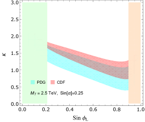
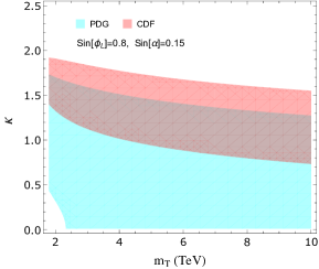
Figure 2: The regions satisfied the precision measurements at $99\%$ C.L. for the bi-doublet scenario with $\Delta M=0.1$ TeV. The green and yellow bands are the same as Figure 1, and the off-perturbation condition is $\sin 2\phi_{L}<\frac{6m_{t}}{m_{T}}$.

4.3 Analysis results

With the analytic formulae for $S,T,U$ we can use the precision global fits to explore the allowed parameter space for the SU(4)/Sp(4) CHM. As $U$ is always subdominant to $S$ and $T$ in our model, we can use the $U=0$ fitting contours. The Particle Data Group (2022) Workman:2022ynf gives the following EW global fit without the CDF result:

$$S=-0.01\pm 0.07\,,\quad T=0.04\pm 0.06$$ (77)

with the correlation coefficient of $0.92$. The new CDF measurement of the W mass has been recently included in the fits: for instace in Ref. Strumia:2022qkt it was obtained

$$S=0.06\pm 0.08\,,\quad T=0.15\pm 0.06$$ (78)

with a strong correlation to be $0.95$. We see that the central value for $T$ is significantly shifted towards positive value, while $S$ received a much less significant shift.

We will start with an order estimation to see whether a CHM is compatible with EW global fit. Differently from the VLQ model, in a CHM we will not work in the limit of small $\sin\phi_{L/R}$ as $M_{5}\sim g_{L/R}f$. And due to the complexity of gauge misalignment effect, normally, it is not easy to perform simplification for $S$ and $T$. While the singlet scenario is an exception, applying the large $M$ expansion to Eq.(64-65) gives:

$$\Delta_{T_{D,mix}} \simeq \frac{3}{8\pi\sin^{2}\theta_{W}\cos^{2}\theta_{W}}\frac{\cos^{2}\phi_{R}}{\sin^{2}\phi_{R}}\frac{y_{t}^{2}}{y_{\tilde{T}}}\left(\log\frac{y_{\tilde{T}}}{y_{t}}-1\right)$$ (79)

$$\Delta_{S_{D,mix}} \simeq \frac{1}{6\pi}\frac{\cos^{2}\phi_{R}}{\sin^{2}\phi_{R}}\frac{y_{t}}{y_{\tilde{T}}}\left(2\log\frac{y_{\tilde{T}}}{y_{t}}-5\right)$$ (80)

The misalignment effect in the $D_{1}$ scenario can also be remarkably simplified if $M_{Q}=M_{T_{1}}$ and in that degenerate limit, we have:

$$\Delta_{S_{D,mis}} \simeq \frac{2\sin^{2}\alpha}{3\pi}(1-\kappa^{2})\left(3\log\frac{\Lambda^{2}}{m_{Q}^{2}}-2\right)$$ (81)

Note that Eq.(79-81) achieve high level precision with respect to original expressions. For $m_{Q/\tilde{T}}\sim 2.0$ TeV, the estimation gives $\Delta_{T_{D,mix}}\sim 0.07\times\frac{\cos^{2}\phi_{R}}{\sin^{2}\phi_{R}}$ and $\Delta_{S_{D,mis}}\sim 0.03\times(1-\kappa^{2})$, with other contributions one order smaller. For the bi-doublet scenario, we first simplify $\Delta_{T_{mis}}$ by keeping the dominant terms:

$$\Delta_{T_{mis}} \simeq \frac{3y_{t}\sin^{2}\phi_{L}\sin^{2}\frac{\alpha}{2}}{8\pi\sin^{2}\theta_{W}\cos^{2}\theta_{W}}\left[(1-\kappa^{2})\log\left(\frac{\Lambda^{2}}{m_{Z}^{2}}\right)+2\kappa^{2}\log\left(\frac{y_{T_{1}}}{y_{t}}\right)\right]$$ (82)

This approximation is in lower precision and positive for $\kappa<1$. Analogously for $m_{T_{1}}\sim 2.0$ TeV, we find $\Delta_{T_{mis}}\sim(7-\kappa^{2})\times 10^{-2}\sin^{2}\phi_{L}$, and $\sin\phi_{L}$ is required to be large enough to compete with the negative one from $\Delta T_{h}$. Regarding $\Delta S$ from top partners, the misalignment part is one order larger than the mixing one if the divergence term is not suppressed. Then for $\sin\phi_{L}\ll 1$ and $M_{T/T_{X}}=M_{T_{1}}$, $\Delta_{S_{mis}}$ in the bi-doublet scenario just reduces to Eq.(81). But for $m_{T}\sim 2.0$ TeV and $\sin\phi_{L}\sim 0.8$ (index of mass splitting), the precise value from Eq.(75) is enhanced by around $25\%$ in magnitude compared with using $m_{T}$ in Eq.(81). Hence the rough evaluation indicates that within $3\sigma$ C.L. both the singlet and bi-doublet scenarios can accommodate the positive shifts in CDF measurement. In the following, we will deliver a two-parameter $\chi^{2}$ analysis, by inputting the accurate $S,T$ expressions.

In Figure 1, we display the constraint of precision measurement on the parameter space for the $D_{1}$ singlet scenario, with the 99% C.L. region permitted by PDG (2022) shown by the cyan band, and the region including CDF by the red one. Since all the contours are insensitive to the mass difference of $M_{5}-M_{1}$, we set $\Delta M=100$ GeV in the plots. Provided that the singlet top partner $\tilde{T}$ is not too heavy, the positive contribution in Eq. (64) can overcome the small negative one from the reduced Higgs coupling. However, $\Delta T_{\rm mix}$ in Eq. (64) is inversely proportional to $\sin^{2}\phi_{R}$ in both $D_{1}$ or $A_{1}$ embeddings, thus for a small $\sin\phi_{R}$ the overall positive correction is too big to fit into the electroweak precision data. This characteristic behaviour is manifested in Figure 1(a) and 1(b). Also the logarithmic divergence in $\Delta S_{D(A),\text{mis}}$ will turn into dominantly negative as the value of $\kappa$ increases, this will translate into an upper bound for the $\kappa$ coefficient as shown in Figure 1(a)- 1(d). We can find out the $\kappa$ is mainly constrained to be $\mathcal{O}(1)$ with the CDF global fit preferring a larger $\kappa$ in the same set of other inputs. Notice that the shape of the allowed region changes dramatically between Figure 1(c) and Figure 1(d), which shows that enhancing the LO mixing $\sin\phi_{R}$ can alleviate the lower bound of $m_{T}$. It should be noted that top partner masses in the multi-TeV scale, as preferred by Lattice data, can well fit within the EW precision limits.

For comparison, the constraints from the EW global fit is also imposed on the bi-doublet scenario, as shown in Figure 2. We find that the pattern of the plots is mainly determined by the $T$ parameter, while the $S$ parameter simply drags $\kappa$ toward smaller values due to the logarithmic term. More in detail, we see that the first term in $\Delta T_{\rm mis}$ in Eq. (74) is always positive for a TeV scale top partner and plays the same role as the singlet mixing contribution. Instead, the term of the second line in Eq. (74) (including the logarithmic and finite terms) will transit from positive to negative at the point of $\kappa=\frac{1}{\cos\frac{\alpha}{2}}$. Thus, $\Delta T_{\rm mis}$ in Eq. (74), stemming from the misalignment, is positive for relatively small $\kappa$ and large $m_{T_{1}}$. In contrast to the singlet case in Eq. (64), the coefficient of the positive term is proportional to $\sin^{2}\phi_{L}$. Therefore, in order to compete with the negative contribution from the Higgs couplings in Eq. (63), a minimum value of $\sin\phi_{L}$ is determined either by the $T$ parameter lower bound or by the perturbation constraint in Eq. (59). For large $\sin\phi_{L}$, However, due to a reduction in $m_{T_{1}}=m_{T}\sqrt{1-\sin^{2}\phi_{L}}-\Delta M$, the first positive term in Eq. (74) can become smaller than the negative logarithmic term for $\kappa>\frac{1}{\cos\frac{\alpha}{2}}$. This will lead to the exclusion of some upper region in Figure 2(a). The same pattern is exhibited in Figure 2(b), where the allowed region shrinks due to a larger $\sin\alpha$. Figure 2(c) shows the allowed region in the $(m_{T},\kappa)$ space, where for $\sin\phi_{L}=0.3$, the $T$ parameter is only positive for a large $m_{T}$, while in Figure 2(d) with $\sin\phi_{L}=0.8$, the allowed $\kappa$ value is significantly lowered.

5 Discussion and conclusions

Composite Higgs models with top partial compositeness offer a valid alternative to the Higgs sector of the SM, as they solve the hierarchy problem in the Higgs mass by replacing an elementary scalar field by a composite state of fermions. In the recent years, this possibility has risen to the level of one of the main models for new physics to be searched for at collider experiments. Besides direct searches for resonances in the electroweak and top sectors, this class of models predicts distinctive modifications to electroweak precision observables.

In this work, after reviewing some universal property in CHM, we revisited the contribution of top partners to electroweak precision via the oblique $S$ and $T$ parameters. We identified a new contribution stemming from misalignment effects that modify the gauge couplings of the top partners to the $W$ and $Z$ bosons. Contrary to the usual mixing effects, these contributions can be logarithmically divergent and hence numerically large. For concreteness, we computed them explicitly in the minimal model with an underlying gauge-fermion description, based on the coset SU(4)/Sp(4). Nevertheless, we only consider simplified mixing patterns involving either a singlet or a custodial bi-doublet, henceforth the results can be generalised to other cosets in this limit. The singlet case can naturally accommodate a positive shift on $T$. For the bi-doublet case, where a negative $T$ from reduced Higgs coupling is not compensated by the basis rotation, but the misalignment effects can shift the $T$ parameter towards positive value, as suggested by the recent CDF measurement of the $W$ mass. In this case, an order unity derivative coupling of the pNGBs to the top partners is required.

In general, we see that the misalignment contribution is crucial for a correct estimation of the impact of top partial compositeness on electroweak precision. In particular, the effect of the derivative couplings can dominate and push the $T$ parameters towards positive values. Furthermore, masses for the top partners in the multi-TeV are compatible with the new CDF measurement, which requires a sizeable positive shift in $T$. This scenario will be tested in future colliders via precision measurements at the $e+e-$ run and direct searches for top partners at the 100 TeV hadronic run.

Appendix A Oblique parameters: $S,T$ and $U$

In this section, we will show how to derive the vacuum polarization amplitude with VLQ running in the loop that are used in the oblique parameters. Let us denote the up and down-type quarks as $\psi^{u}$, $\psi^{d}$ and fermions of exotic charges $Q=\frac{5}{3}$ as $X_{u}$ or $Q=-\frac{4}{3}$ as $X_{d}$. The Lagrangian of $\psi^{u,d}$ coupling to a gauge boson $W_{\mu}^{\pm,3},B_{\mu}$ in the mass basis reads:

$$\mathcal{L}_{1} = \frac{g_{2}}{\sqrt{2}}\left[W_{\mu}^{+}\bar{\psi}^{u}_{\alpha}\gamma^{\mu}\left(V_{L,\alpha i}P_{L}+V_{R,\alpha i}P_{R}\right)\psi^{d}_{i}\right]+h.c.$$ (83)

$$+ \frac{g_{2}}{2}W_{3\mu}\left[\bar{\psi}_{\alpha}^{u}\gamma^{\mu}\left(U_{L,\alpha\beta}P_{L}+U_{R,\alpha\beta}P_{R}\right)\psi^{u}_{\beta}-\bar{\psi^{d}_{i}}\gamma^{\mu}\left(D_{L,ij}P_{L}+D_{R,ij}P_{R}\right)\psi^{d}_{j}\right]$$

$$+ g_{1}B_{\mu}\left[\bar{\psi}_{\alpha}^{u}\gamma^{\mu}\left(Y_{L,\alpha\beta}^{u}P_{L}+Y_{R,\alpha\beta}^{u}P_{R}\right)\psi^{u}_{\beta}+\bar{\psi}^{d}_{i}\gamma^{\mu}\left(Y_{L,ij}^{d}P_{L}+Y_{R,ij}^{d}P_{R}\right)\psi^{d}_{j}\right]$$

with $P_{L/R}=\frac{1}{2}(1\mp\gamma_{5})$. Since the VLQ with exotic charges will not mix with SM fermions, their gauge interactions are:

$$\mathcal{L}_{2} = \frac{g_{2}}{\sqrt{2}}W_{\mu}^{+}\left[\bar{X}_{u}\gamma^{\mu}\left(\tilde{V}_{L,\alpha}P_{L}+\tilde{V}_{R,\alpha}P_{R}\right)\psi^{u}_{\alpha}+\bar{\psi}^{d}_{i}\gamma^{\mu}\left(\hat{V}_{L,i}P_{L}+\hat{V}_{R,i}P_{R}\right)X_{d}\right]$$ (84)

$$+ \frac{g_{2}}{2}W_{3\mu}\left[\bar{X}_{u}\gamma^{\mu}U_{X}X_{u}-\bar{X}_{d}\gamma^{\mu}D_{X}X_{d}\right]$$

$$+ \frac{g_{1}}{2}B_{\mu}\left[\bar{X}_{u}\gamma^{\mu}(2Q-U_{X})X_{u}-\bar{X}_{d}\gamma^{\mu}(2Q+D_{X})X_{d}\right]+h.c.$$

One can derive the transverse part of vacuum polarization amplitude to be:

$$A_{VV}(p^{2}=0) = \frac{N_{c}m^{2}_{Z}}{128\pi^{2}}\left[(|g_{L}^{V}|^{2}+|g_{R}^{V}|^{2})\left(A_{0}(m^{2}_{1})+A_{0}(m^{2}_{2})+(m^{2}_{1}+m^{2}_{2})B_{0}(0,m^{2}_{1},m^{2}_{2})\right)\right.$$ (85)

$$\quad\qquad-\left.8\,{\mathcal{R}e}(g_{L}^{V}g_{R}^{V{\dagger}})m_{1}m_{2}B_{0}(0,m^{2}_{1},m^{2}_{2})\right]\,,$$

with the masses of two fermions to be $m_{1,2}$ and the superscript $V$ standing for a specific gauge boson. Note that $g_{L/R}^{V}$ equals one coupling in $(V_{L/R},U_{L/R},-D_{L/R},2Y_{L/R}^{u,d})$ or $(\tilde{V}_{L/R},\hat{V}_{L/R},U_{X},-D_{X},2Y_{X_{u,d}})$. The $A_{0}(m^{2})$ and $B_{0}(p^{2},m_{1}^{2},m_{2}^{2})$ are rescaled Veltman scalar loop functions tHooft:1978jhc ; Passarino:1978jh . For $p^{2}=0$, the dimensional regularization gives:

$$A_{0}(m^{2})=m^{2}(\Delta+1-\log\frac{m^{2}}{\mu^{2}})\,,\quad B_{0}(0,m^{2}_{1},m^{2}_{2})=\frac{A_{0}(m^{2}_{1})-A_{0}(m^{2}_{2})}{m^{2}_{1}-m^{2}_{2}}\,$$ (86)

with $\Delta=\frac{2}{4-d}+\log 4\pi+\gamma_{E}$. The pole at $d=4$ represents the logarithmic divergence. Using the momentum cut-off regularization, one can calculate:

$$B_{0}(0,m^{2},m^{2})=\frac{(2\pi\mu)^{4-d}}{i\pi^{2}}\int\frac{d^{4}k}{(k^{2}-m^{2})^{2}}=\log\frac{\Lambda^{2}}{m^{2}}-1$$ (87)

directly matching Eq.(86) with Eq.(87) we get:

$$\Delta+\log\mu^{2}+1=\log\Lambda^{2}\,,$$ (88)

By substituting Eq.(86, 88) into Eq.(85), we can simplify the expression to be:

$$A_{VV}(p^{2}=0) = \frac{N_{c}m^{2}_{Z}}{128\pi^{2}}\Big{[}(|g_{L}^{V}|^{2}+|g_{R}^{V}|^{2})\,\theta_{+}(y_{1},y_{2})+2\,{\mathcal{R}e}(g_{L}^{V}g_{R}^{V{\dagger}})\,\theta_{-}(y_{1},y_{2})$$ (89)

$$+ (|g_{L}^{V}|^{2}+|g_{R}^{V}|^{2})\Big{[}(y_{1}+y_{2})\left(\log\frac{\Lambda^{2}}{m^{2}_{Z}}-\frac{1}{2}\right)-2\left(y_{1}\log y_{1}+y_{2}\log y_{2}\right)\Big{]}$$

$$+ 4\,{\mathcal{R}e}(g_{L}^{V}g_{R}^{V{\dagger}})\sqrt{y_{1}y_{2}}\Big{[}\log(y_{1}y_{2})-2\left(\log\frac{\Lambda^{2}}{m^{2}_{Z}}-1\right)\Big{]}\Big{]}$$

with $y_{i}=m_{i}^{2}/m_{Z}^{2}$ being dimensionless and $\theta_{\pm}$ defined to be Lavoura:1992np :

$$\theta_{+}(y_{1},y_{2}) = y_{1}+y_{2}-\frac{2y_{1}y_{2}\log\left(\frac{y_{1}}{y_{2}}\right)}{y_{1}-y_{2}}$$ (90)

$$\theta_{-}(y_{1},y_{2}) = 2\sqrt{y_{1}y_{2}}\left(\frac{(y_{1}+y_{2})\log\left(\frac{y_{1}}{y_{2}}\right)}{y_{1}-y_{2}}-2\right)$$ (91)

Because the term proportional to $|g_{L}^{V}|^{2}+|g_{R}^{V}|^{2}$ gets additional contribution from $A_{0}$ functions compared with the one proportional to ${\mathcal{R}e}(g_{L}^{V}g_{R}^{V{\dagger}})$, two divergence structures are different. Then we can calculate the derivative of $A_{VV^{\prime}}$ to be:

$$\frac{\partial A_{VV^{\prime}}}{\partial p^{2}}|_{p^{2}=0} = \frac{N_{c}}{96\pi^{2}}\left[(g_{L}^{V}g_{L}^{V^{\prime}{\dagger}}+g_{R}^{V}g_{R}^{V^{\prime}{\dagger}})\Big{[}\frac{(m^{2}_{1}-m^{2}_{2})^{2}}{4}\,\frac{\partial^{2}B_{0}(p^{2},m^{2}_{1},m^{2}_{2})}{\partial^{2}p^{2}}|_{p^{2}=0}\right.$$ (92)

$$+ \left.\frac{m^{2}_{1}+m^{2}_{2}}{2}\,\frac{\partial B_{0}(p^{2},m^{2}_{1},m^{2}_{2})}{\partial p^{2}}|_{p^{2}=0}-B_{0}(0,m^{2}_{1},m^{2}_{2})\Big{]}\right.$$

$$- \left.3(g_{L}^{V}g_{R}^{V^{\prime}{\dagger}}+g_{R}^{V}g_{L}^{V^{\prime}{\dagger}})m_{1}m_{2}\,\frac{\partial B_{0}(p^{2},m^{2}_{1},m^{2}_{2})}{\partial p^{2}}|_{p^{2}=0}\right]$$

using the dimensional regularization, the two-point loop function $B_{0}$ takes the form:

$$B_{0}(p^{2},m^{2}_{1},m^{2}_{2})=\Delta-\int^{1}_{0}dx\log\left[\frac{m^{2}_{1}x+m^{2}_{2}(1-x)-p^{2}x(1-x)}{\mu^{2}}-i\varepsilon\right]$$ (93)

The derivatives of $B_{0}$ are all finite and can be evaluated analytically to be:

$$\frac{\partial B_{0}(p^{2},m^{2}_{1},m^{2}_{2})}{\partial p^{2}}|_{p^{2}=0} = \frac{m_{1}^{4}-m_{2}^{4}-2m_{1}^{2}m_{2}^{2}\log\frac{m_{1}^{2}}{m_{2}^{2}}}{2\left(m_{1}^{2}-m_{2}^{2}\right)^{3}}$$ (94)

$$\frac{\partial^{2}B_{0}(p^{2},m^{2}_{1},m^{2}_{2})}{\partial^{2}p^{2}}|_{p^{2}=0} = \frac{(m^{2}_{1}+m^{2}_{2})^{2}+8m^{2}_{1}m^{2}_{2}}{3(m^{2}_{1}-m^{2}_{2})^{4}}$$ (95)

$$- \frac{2m^{2}_{1}m_{2}^{2}\left(m_{1}^{2}+m_{2}^{2}\right)\log\left(\frac{m_{1}^{2}}{m_{2}^{2}}\right)}{\left(m_{1}^{2}-m_{2}^{2}\right)^{5}}\,$$

In fact this approach avoids the integration complexity confronted in the average slope method adopted byLavoura:1992np . Now inserting Eq.(86, 94-95), we obtain

$$\frac{\partial A_{VV^{\prime}}}{\partial p^{2}}|_{p^{2}=0} = -\frac{N_{c}}{64\pi^{2}}\Big{[}(g_{L}^{V}g_{L}^{V^{\prime}{\dagger}}+g_{R}^{V}g_{R}^{V^{\prime}{\dagger}})\left(\chi_{+}(y_{1},y_{2})-\frac{1}{3}\log(y_{1}y_{2})+\frac{2}{3}\left(\log\frac{\Lambda^{2}}{m_{Z}^{2}}-\frac{7}{6}\right)\right)$$ (96)

$$+ (g_{L}^{V}g_{R}^{V^{\prime}{\dagger}}+g_{R}^{V}g_{L}^{V^{\prime}{\dagger}})\Big{(}\chi_{-}(y_{1},y_{2})-\psi_{-}(y_{1},y_{2})\Big{)}\Big{]}\,,$$

Note that our result only differs from Lavoura:1992np in the third term of the first line. One will get a wrong constant term $\frac{G_{V}+G_{A}}{24\pi^{2}}$ from Eq.(14) in Lavoura:1992np , by taking the limit of $\frac{y_{i}}{\epsilon}|_{\epsilon\to 0}$ for conversion into derivative. The definitions of $\chi_{\pm}$ and $\psi_{-}$ are:

$$\chi_{+}(y_{1},y_{2}) = \frac{\left(3y_{1}y_{2}(y_{1}+y_{2})-y_{1}^{3}-y_{2}^{3}\right)\log\left(\frac{y_{1}}{y_{2}}\right)}{3(y_{1}-y_{2})^{3}}+\frac{5\left(y_{1}^{2}+y_{2}^{2}\right)-22y_{1}y_{2}}{9(y_{1}-y_{2})^{2}}$$ (97)

$$\chi_{-}(y_{1},y_{2}) = -\sqrt{y_{1}y_{2}}\left(\frac{y_{1}+y_{2}}{6y_{1}y_{2}}-\frac{y_{1}+y_{2}}{(y_{1}-y_{2})^{2}}+\frac{2y_{1}y_{2}\log\left(\frac{y_{1}}{y_{2}}\right)}{(y_{1}-y_{2})^{3}}\right)$$ (98)

$$\psi_{-}(y_{1},y_{2}) = -\frac{y_{1}+y_{2}}{6\sqrt{y_{1}y_{2}}}$$ (99)

With the formulas of Eq.(89, 96), the oblique parameters $S,T,U$ can be calculated straightforward in a generic model and the divergence will only show up when the unitarity is violated, e.g. by the misalignment in CHM discussed in the main text. As an application, we consider a simplified case without divergence, where VLQ is embedded in an irreducible representation of $SU(2)_{L}\times U(1)_{Y}$ and interplays with SM fermions via a Higgs VEV insertion. From Eq.(96), the $S$ parameter is computed by summing over all fermion contribution:

$$S = -16\pi\sum_{\{\psi,X\}}\partial A_{3Y}/\partial p^{2}|_{p^{2}=0}$$ (100)

$$= \frac{N_{c}}{2\pi}\Big{[}\sum_{ij}{\mathcal{R}e}(D_{L,ij}D_{R,ij}^{*})\psi_{-}(y_{i},y_{j})+\sum_{\alpha\beta}{\mathcal{R}e}(U_{L,\alpha\beta}U_{R,\alpha\beta}^{*})\psi_{-}(y_{\alpha},y_{\beta})$$

$$- \sum_{\alpha<\beta}\Big{[}\left(|U_{L,\alpha\beta}|^{2}+|U_{R,\alpha\beta}|^{2}\right)\chi_{+}(y_{\alpha},y_{\beta})+2{\mathcal{R}e}(U_{L,\alpha\beta}U_{R,\alpha\beta}^{*})\chi_{-}(y_{\alpha},y_{\beta})\Big{]}$$

$$- \sum_{i<j}\Big{[}\left(|D_{L,ij}|^{2}+|D_{R,ij}|^{2}\right)\chi_{+}(y_{i},y_{j})+2{\mathcal{R}e}(D_{L,ij}D_{R,ij}^{*})\chi_{-}(y_{i},y_{j})\Big{]}$$

$$- \frac{1}{3}\Big{[}\sum_{\alpha}Q_{\alpha}\left(U_{L,\alpha\alpha}+U_{R,\alpha\alpha}\right)\Big{(}\log(y_{\alpha}^{2})-1\Big{)}-\sum_{i}Q_{i}\left(D_{L,ii}+D_{R,ii}\right)\Big{(}\log(y_{i}^{2})-1\Big{)}\Big{]}$$

$$+ \frac{1}{6}\Big{[}\sum_{\alpha\beta}\left(|U_{L,\alpha\beta}|^{2}+|U_{R,\alpha\beta}|^{2}\right)\log(y_{\alpha}y_{\beta})+\sum_{ij}\left(|D_{L,ij}|^{2}+|D_{R,ij}|^{2}\right)\log(y_{i}y_{j})\Big{]}$$

$$- \frac{1}{3}\Big{[}U_{X}(2Q_{X_{u}}-U_{X})\Big{(}\log(y_{X_{u}}^{2})-1\Big{)}-D_{X}(2Q_{X_{d}}+D_{X})\Big{(}\log(y_{X_{d}}^{2})-1\Big{)}\Big{]}\Big{]}$$

Using the condition that terms proportional to $(y_{a}\log y_{a}+y_{b}\log y_{b})$ along with the divergence $(y_{a}+y_{b})\left(\log\frac{\Lambda^{2}}{m_{Z}^{2}}-\frac{1}{2}\right)$ in the expression of $T$ parameter will vanish, we can derive that:

$$\sum_{i}\left(|V_{L,\alpha i}|^{2}+|V_{R,\alpha i}|^{2}\right)+\left(\tilde{V}_{L,\alpha}^{2}+\tilde{V}_{R,\alpha}^{2}\right)=\sum_{\beta}\left(|U_{L,\alpha\beta}|^{2}+|U_{R,\alpha\beta}|^{2}\right)$$ (101)

$$\sum_{\alpha}\left(|V_{L,\alpha i}|^{2}+|V_{R,\alpha i}|^{2}\right)+\left(\hat{V}_{L,i}^{2}+\hat{V}_{R,i}^{2}\right)=\sum_{j}\left(|D_{L,ij}|^{2}+|D_{R,ij}|^{2}\right)$$ (102)

$$\sum_{\alpha}\left(\tilde{V}_{L,\alpha}^{2}+\tilde{V}_{R,\alpha}^{2}\right)=2U_{X}^{2}\,,\quad\sum_{i}\left(\hat{V}_{L,i}^{2}+\hat{V}_{R,i}^{2}\right)=2D_{X}^{2}$$ (103)

Similarly in the $T$ parameter, Requiring that terms proportional to $\sqrt{y_{a}y_{b}}\log(y_{a}y_{b})$ to be cancelled will lead to:

$$\sum_{i}{\mathcal{R}e}(V_{L,\alpha i}V_{R,\alpha i}^{*})\sqrt{y_{i}}+{\mathcal{R}e}(\tilde{V}_{L,\alpha}\tilde{V}_{R,\alpha}^{*})\sqrt{y_{X_{u}}}=\sum_{\beta}{\mathcal{R}e}(U_{L,\alpha\beta}U_{R,\alpha\beta}^{*})\sqrt{y_{\beta}}$$ (104)

$$\sum_{\alpha}{\mathcal{R}e}(V_{L,\alpha i}V_{R,\alpha i}^{*})\sqrt{y_{\alpha}}+{\mathcal{R}e}(\hat{V}_{L,i}\hat{V}_{R,i}^{*})\sqrt{y_{X_{d}}}=\sum_{j}{\mathcal{R}e}(D_{L,ij}D_{R,ij}^{*})\sqrt{y_{j}}$$ (105)

$$\sum_{\alpha}{\mathcal{R}e}(\tilde{V}_{L,\alpha}\tilde{V}_{R,\alpha}^{*})\sqrt{y_{\alpha}}=U_{X}^{2}\sqrt{y_{X_{u}}}\,,\quad\sum_{i}{\mathcal{R}e}(\hat{V}_{L,i}\hat{V}_{R,i}^{*})\sqrt{y_{i}}=D_{X}^{2}\sqrt{y_{X_{d}}}$$ (106)

that are general results for VLQ in an irreducible representation, and we have explicitly verified that these sum rules are observed in the non-standard doublet ($Y=\frac{7}{6},-\frac{5}{6}$) and triplet scenarios ($Y=\frac{2}{3},-\frac{1}{3}$). This class of models also satisfy the following relations:

$$U_{L/R}=V_{L/R}V_{L/R}^{\dagger}-\tilde{V}_{L/R}^{\dagger}\tilde{V}_{L/R}\,,\quad D_{L/R}=V_{L/R}^{\dagger}V_{L/R}-\hat{V}_{L/R}\hat{V}_{L/R}^{\dagger}$$

$$U_{X}=\tilde{V}_{L/R}\tilde{V}_{L/R}^{\dagger}\,,\quad D_{X}=\hat{V}_{L/R}^{\dagger}\hat{V}_{L/R}$$ (107)

Then applying Eq.(107) and Eq.(101-103), we can rearrange most of the terms other than $\chi_{\pm}$ and $\psi_{-}$ in Eq.(100) into a new function $\psi_{+}$ that is defined as:

$$\psi_{+}(y_{a},y_{b})=\frac{1}{3}\left(Q_{a}-Q_{b}\right)-\frac{1}{3}\left(Q_{a}+Q_{b}\right)\log\left(\frac{y_{a}}{y_{b}}\right)$$ (108)

Note that $\psi_{+}$ is antisymmetric for exchanging $(y_{a},y_{b})$ and in fact $Q_{a}-Q_{b}=\pm 1$ always holds due to the $W^{\pm}_{\mu}$ current. The structure inside the logarithm is expected since the divergence in $S$ parameter vanishes due to unitarity conservation. Also using Eq.(104-106), we can conduct a transformation for the expression:

$$\sum_{ij}{\mathcal{R}e}(D_{L,ij}D_{R,ij}^{*})\psi_{-}(y_{i},y_{j})+\sum_{\alpha\beta}{\mathcal{R}e}(U_{L,\alpha\beta}U_{R,\alpha\beta}^{*})\psi_{-}(y_{\alpha},y_{\beta})-\frac{1}{3}\left(U_{X}^{2}+D_{X}^{2}\right)$$ (109)

$$= 2\sum_{\alpha i}{\mathcal{R}e}(V_{L,\alpha i}V_{R,\alpha i}^{*})\psi_{-}(y_{\alpha},y_{i})+2\sum_{\alpha}{\mathcal{R}e}(\tilde{V}_{L,\alpha}\tilde{V}_{R,\alpha}^{*})\psi_{-}(y_{X_{u}},y_{\alpha})$$

$$+ 2\sum_{i}{\mathcal{R}e}(\hat{V}_{L,i}\hat{V}_{R,i}^{*})\psi_{-}(y_{i},y_{X_{d}})$$

Thus the general formula for $S$ parameter originating from mixing with VLQ in an irreducible representation is:

$$S = \frac{N_{c}}{2\pi}\Big{[}\sum_{\alpha i}\left[\left(|V_{L,\alpha i}|^{2}+|V_{R,\alpha i}|^{2}\right)\psi_{+}(y_{\alpha},y_{i})+2{\mathcal{R}e}(V_{L,\alpha i}V_{R,\alpha i}^{*})\psi_{-}(y_{\alpha},y_{i})\right]$$ (110)

$$+ \sum_{\alpha}\left[\left(|\tilde{V}_{L,\alpha}|^{2}+|\tilde{V}_{R,\alpha}|^{2}\right)\psi_{+}(y_{X_{u}},y_{\alpha})+2{\mathcal{R}e}(\tilde{V}_{L,\alpha}\tilde{V}_{R,\alpha}^{*})\psi_{-}(y_{X_{u}},y_{\alpha})\right]$$

$$+ \sum_{i}\left[\left(|\hat{V}_{L,i}|^{2}+|\hat{V}_{R,i}|^{2}\right)\psi_{+}(y_{i},y_{X_{d}})+2{\mathcal{R}e}(\hat{V}_{L,i}\hat{V}_{R,i}^{*})\psi_{-}(y_{i},y_{X_{d}})\right]$$

$$- \sum_{\alpha<\beta}\left[\left(|U_{L,\alpha\beta}|^{2}+|U_{R,\alpha\beta}|^{2}\right)\chi_{+}(y_{\alpha},y_{\beta})+2{\mathcal{R}e}(U_{L,\alpha\beta}U_{R,\alpha\beta}^{*})\chi_{-}(y_{\alpha},y_{\beta})\right]$$

$$- \sum_{i<j}\left[\left(|D_{L,ij}|^{2}+|D_{R,ij}|^{2}\right)\chi_{+}(y_{i},y_{j})+2{\mathcal{R}e}(D_{L,ij}D_{R,ij}^{*})\chi_{-}(y_{i},y_{j})\right]\Big{]}$$

where $(\alpha,\beta)$ specify the up-type quarks and $(i,j)$ are for the down-type quarks. This generalizes the result in Ref.Lavoura:1992np .

Appendix B Model detail

We first report the gauge-fermion couplings that are relevant to the $S,T,U$ calculation. Note that the couplings below are not rotated into the mass basis. For the fiveplet $\psi_{5}$, the gauge interaction is constructed from the CCWZ object, but we can separate out the part without misalignment to be:

$$Tr\left[\bar{\psi}_{5}\gamma^{\mu}\left(V_{\mu}\psi_{5}+\psi_{5}V_{\mu}^{T}\right)+g_{1}B_{\mu}^{0}\hat{X}\bar{\psi}_{5}\gamma^{\mu}\psi_{5}\right]$$ (111)

$$= \frac{g_{2}}{2}\Big{[}W_{1}^{\mu}\left(\bar{T}\gamma_{\mu}B+\bar{X}\gamma_{\mu}T_{X}\right)-iW_{2}^{\mu}\left(\bar{T}\gamma_{\mu}B+\bar{X}\gamma_{\mu}T_{X}\right)+h.c.$$

$$+ W_{3}^{\mu}\left(\bar{T}\gamma_{\mu}T-\bar{B}\gamma_{\mu}B+\bar{X}\gamma_{\mu}X-\bar{T}_{X}\gamma_{\mu}T_{X}\right)$$

$$+ \frac{1}{6}B_{0}^{\mu}\tan(\text{$\theta$w})\left(\bar{T}\gamma_{\mu}T+\bar{B}\gamma_{\mu}B+7\bar{X}\gamma_{\mu}X+7\bar{T}_{X}\gamma_{\mu}T_{X}\right)\Big{]}$$

with $V_{\mu}=g_{2}W_{\mu}^{i}T_{L}^{i}+g_{1}B_{\mu}T_{R}^{3}$. The pure misaligned term encoded in the $\delta E_{\mu}=E_{\mu}-V_{\mu}$ part can be expanded to be:

$$Tr\left[\bar{\psi}_{5}\gamma^{\mu}\left(\delta E_{\mu}\psi_{5}+\psi_{5}\delta E_{\mu}^{T}\right)\right]\supset$$ (112)

$$- \frac{g_{2}\sin^{2}\left(\frac{\alpha}{2}\right)}{2}\Big{[}W_{1}^{\mu}\left(\bar{B}+\bar{X}\right)\gamma_{\mu}\left(T+T_{X}\right)+iW_{2}^{\mu}\left(\bar{B}-\bar{X}\right)\gamma_{\mu}\left(T+T_{X}\right)$$

$$+ 2W_{3}^{\mu}\left(\bar{T}\gamma_{\mu}T-\bar{T}_{X}\gamma_{\mu}T_{X}\right)-2B_{0}^{\mu}\tan(\text{$\theta$w})\left(\bar{T}\gamma_{\mu}T-\bar{T}_{X}\gamma_{\mu}T_{X}\right)\Big{]}+h.c.\,$$

The $d_{\mu}$ term without the pNGB derivative coupling is:

$$Tr[\bar{\psi}_{5}d_{\mu}\gamma^{\mu}\psi_{1}]+h.c. \supset \frac{g_{2}\sin(\alpha)}{2\sqrt{2}}\Big{[}W_{1}^{\mu}\left(\bar{B}+\bar{X}\right)+iW_{2}^{\mu}\left(\bar{B}-\bar{X}\right)$$ (113)

$$+ W_{3}^{\mu}\left(\bar{T}-\bar{T}_{X}\right)-B_{0}^{\mu}\tan(\text{$\theta$w})\left(\bar{T}-\bar{T}_{X}\right)\Big{]}\gamma_{\mu}T_{1}+h.c.\,$$

Let us consider the SM $(t_{L},b_{L})$ and $t_{R}$ are embedded in the adjoint spurion, the top partners in $\psi_{5}$ and elementary fermions can be arranged into up and down sectors:

$$\mathcal{U}\equiv\left(t,T,T_{X},\tilde{T}\right)^{T}\,\quad\mathcal{D}\equiv\left(b,B\right)^{T}$$ (114)

To diagonalize the up and down masses, i.e. $\Omega^{\dagger}_{L}M_{2/3}\Omega_{R}=M_{2/3}^{diag}$ and $\Omega^{d{\dagger}}_{L}M_{-1/3}\Omega_{R}^{d}=M_{-1/3}^{diag}$, the rotation for one bi-doublet scenario in Eq.(46) at $\mathcal{O}(\epsilon^{2})$ ($\epsilon\equiv\sin\alpha$) is :

$$\Omega_{L}=\left(\begin{array}[]{cccc}\frac{M_{5}}{\sqrt{M_{5}^{2}+f^{2}y_{L1}^{2}}}&\frac{fy_{L1}}{\sqrt{M_{5}^{2}+f^{2}y_{L1}^{2}}}&0&0\\ -\frac{fy_{L1}}{\sqrt{M_{5}^{2}+f^{2}y_{L1}^{2}}}&\frac{M_{5}}{\sqrt{M_{5}^{2}+f^{2}y_{L1}^{2}}}&0&0\\ 0&0&1&0\\ 0&0&0&1\\ \end{array}\right)$$ (119)

$$+ \epsilon^{2}\left(\begin{array}[]{cccc}\frac{M_{5}f^{2}y_{L1}^{2}\left(f^{2}\left(y_{L1}^{2}+y_{R1}^{2}\right)+M_{5}^{2}\right)}{4\left(M_{5}^{2}+f^{2}y_{L1}^{2}\right)^{5/2}}&-\frac{M_{5}^{2}fy_{L1}\left(f^{2}\left(y_{L1}^{2}+y_{R1}^{2}\right)+M_{5}^{2}\right)}{4\left(M_{5}^{2}+f^{2}y_{L1}^{2}\right)^{5/2}}&\frac{fy_{R1}^{2}}{4M_{5}y_{L1}}&0\\ \frac{M_{5}^{2}fy_{L1}\left(f^{2}\left(y_{L1}^{2}+y_{R1}^{2}\right)+M_{5}^{2}\right)}{4\left(M_{5}^{2}+f^{2}y_{L1}^{2}\right)^{5/2}}&\frac{M_{5}f^{2}y_{L1}^{2}\left(f^{2}\left(y_{L1}^{2}+y_{R1}^{2}\right)+M_{5}^{2}\right)}{4\left(M_{5}^{2}+f^{2}y_{L1}^{2}\right)^{5/2}}&\frac{1}{4}\left(\frac{y_{R1}^{2}}{y_{L1}^{2}}-\frac{f^{2}y_{R1}^{2}}{M_{5}^{2}}-1\right)&0\\ -\frac{\left(M_{5}^{2}+f^{2}y_{R1}^{2}\right)}{4M_{5}^{2}\sqrt{\frac{M_{5}^{2}}{f^{2}y_{L1}^{2}}+1}}&\frac{\left(y_{L1}^{2}-y_{R1}^{2}\right)}{4y_{L1}^{2}\sqrt{\frac{f^{2}y_{L1}^{2}}{M_{5}^{2}}+1}}&0&0\\ 0&0&0&0\\ \end{array}\right)$$ (124)

$$\Omega_{R}=\left(\begin{array}[]{cccc}1-\frac{\epsilon^{2}\left(\frac{M_{5}^{4}}{\left(M_{5}^{2}+f^{2}y_{L1}^{2}\right)^{2}}+1\right)f^{2}y_{R1}^{2}}{8M_{5}^{2}}&-\frac{\epsilon M_{5}fy_{R1}}{2\left(M_{5}^{2}+f^{2}y_{L1}^{2}\right)}&\frac{\epsilon fy_{R1}}{2M_{5}}&0\\ \frac{\epsilon M_{5}fy_{R1}}{2\left(M_{5}^{2}+f^{2}y_{L1}^{2}\right)}&1-\frac{\epsilon^{2}M_{5}^{2}f^{2}y_{R1}^{2}}{8\left(M_{5}^{2}+f^{2}y_{L1}^{2}\right)^{2}}&\frac{\epsilon^{2}}{4}\left(\frac{y_{R1}^{2}}{y_{L1}^{2}}-1\right)&0\\ -\frac{\epsilon fy_{R1}}{2M_{5}}&\frac{\epsilon^{2}}{4}\left(1-\frac{M_{5}^{2}y_{R1}^{2}}{y_{L1}^{2}\left(M_{5}^{2}+f^{2}y_{L1}^{2}\right)}\right)&1-\frac{\epsilon^{2}f^{2}y_{R1}^{2}}{8M_{5}^{2}}&0\\ 0&0&0&1\end{array}\right)$$ (129)

$$\Omega_{L}^{d}=\left(\begin{array}[]{cc}\frac{M_{5}}{\sqrt{M_{5}^{2}+f^{2}y_{L1}^{2}}}&\frac{fy_{L1}}{\sqrt{M_{5}^{2}+f^{2}y_{L1}^{2}}}\\ -\frac{fy_{L1}}{\sqrt{M_{5}^{2}+f^{2}y_{L1}^{2}}}&\frac{M_{5}}{\sqrt{M_{5}^{2}+f^{2}y_{L1}^{2}}}\\ \end{array}\right)+\epsilon^{2}\left(\begin{array}[]{cc}\frac{M_{5}f^{2}y_{L1}^{2}}{2\left(M_{5}^{2}+f^{2}y_{L1}^{2}\right)^{3/2}}&-\frac{M_{5}^{2}fy_{L1}}{2\left(M_{5}^{2}+f^{2}y_{L1}^{2}\right)^{3/2}}\\ \frac{M_{5}^{2}fy_{L1}}{2\left(M_{5}^{2}+f^{2}y_{L1}^{2}\right)^{3/2}}&\frac{M_{5}f^{2}y_{L1}^{2}}{2\left(M_{5}^{2}+f^{2}y_{L1}^{2}\right)^{3/2}}\end{array}\right)$$ (134)

and $\Omega^{d}_{R}=1_{2\times 2}$. The rotation for one singlet scenario in Eq.(46) is:

$$\Omega_{L}=\left(\begin{array}[]{cccc}1-\frac{\epsilon^{2}M_{5}^{2}f^{2}y_{L2}^{2}}{4\left(M_{5}^{2}+f^{2}y_{R2}^{2}\right)^{2}}&0&0&-\frac{\epsilon M_{5}fy_{L2}}{\sqrt{2}\left(M_{5}^{2}+f^{2}y_{R2}^{2}\right)}\\ 0&1&0&0\\ 0&0&1&0\\ \frac{\epsilon M_{5}fy_{L2}}{\sqrt{2}\left(M_{5}^{2}+f^{2}y_{R2}^{2}\right)}&0&0&1-\frac{\epsilon^{2}M_{5}^{2}f^{2}y_{L2}^{2}}{4\left(M_{5}^{2}+f^{2}y_{R2}^{2}\right)^{2}}\end{array}\right)$$ (139)

$$\Omega_{R}=\left(\begin{array}[]{ccccc}\frac{M_{5}}{\sqrt{M_{5}^{2}+f^{2}y_{R2}^{2}}}&0&0&\frac{fy_{R2}}{\sqrt{M_{5}^{2}+f^{2}y_{R2}^{2}}}\\ 0&1&0&0\\ 0&0&1&0\\ -\frac{fy_{R2}}{\sqrt{M_{5}^{2}+f^{2}y_{R2}^{2}}}&0&0&\frac{M_{5}}{\sqrt{M_{5}^{2}+f^{2}y_{R2}^{2}}}\end{array}\right)$$ (144)

$$+ \epsilon^{2}\left(\begin{array}[]{cccc}\frac{M_{5}^{3}f^{2}y_{R2}^{2}\left(f^{2}\left(y_{L2}^{2}+y_{R2}^{2}\right)+M_{5}^{2}\right)}{2\left(M_{5}^{2}+f^{2}y_{R2}^{2}\right)^{7/2}}&0&0&-\frac{M_{5}^{4}fy_{R2}\left(f^{2}\left(y_{L2}^{2}+y_{R2}^{2}\right)+M_{5}^{2}\right)}{2\left(M_{5}^{2}+f^{2}y_{R2}^{2}\right)^{7/2}}\\ 0&0&0&0\\ 0&0&0&0\\ \frac{M_{5}^{4}fy_{R2}\left(f^{2}\left(y_{L2}^{2}+y_{R2}^{2}\right)+M_{5}^{2}\right)}{2\left(M_{5}^{2}+f^{2}y_{R2}^{2}\right)^{7/2}}&0&0&\frac{M_{5}^{3}f^{2}y_{R2}^{2}\left(f^{2}\left(y_{L2}^{2}+y_{R2}^{2}\right)+M_{5}^{2}\right)}{2\left(M_{5}^{2}+f^{2}y_{R2}^{2}\right)^{7/2}}\end{array}\right)$$ (149)

Note that the rotation conserves the unitarity: $\Omega_{L}^{\dagger}\Omega_{L}=\Omega_{L}^{d{\dagger}}\Omega_{L}^{d}=\Omega_{R}\Omega_{R}^{\dagger}=1+\mathcal{O}(\epsilon^{3})$.

We listed the generators for the $SU(4)/Sp(4)$ model below, in particular $X^{1,\cdots 4}$ forms a bi-doublet in $SU(2)_{L}\times SU(2)_{R}$.

$$~{}~{}S^{i}=\frac{1}{2}\left(\begin{array}[]{cc}\sigma_{i}&0\\ 0&0\end{array}\right)\,,\qquad\qquad S^{i+3}=\frac{1}{2}\left(\begin{array}[]{cc}0&0\\ 0&-\sigma_{i}^{T}\end{array}\right)\,,\quad i=\{1,2,3\}$$ (154)

$$S^{7}=\frac{i}{2\sqrt{2}}\left(\begin{array}[]{cc}0&\sigma_{3}\\ -\sigma_{3}&0\end{array}\right)\,,\qquad S^{8}=\frac{1}{2\sqrt{2}}\left(\begin{array}[]{cc}0&1_{2}\\ 1_{2}&0\end{array}\right)\,,$$ (159)

$$S^{9}=\frac{i}{2\sqrt{2}}\left(\begin{array}[]{cc}0&\sigma_{1}\\ -\sigma_{1}&0\end{array}\right)\,,\qquad S^{10}=\frac{i}{2\sqrt{2}}\left(\begin{array}[]{cc}0&\sigma_{2}\\ -\sigma_{2}&0\end{array}\right)\,.$$ (164)

$$X^{1}=-\frac{1}{2\sqrt{2}}\left(\begin{array}[]{cc}0&\sigma_{3}\\ \sigma_{3}&0\end{array}\right)\,,\quad X^{2}=\frac{i}{2\sqrt{2}}\left(\begin{array}[]{cc}0&1_{2}\\ -1_{2}&0\end{array}\right)\,,\quad X^{3}=\frac{1}{2\sqrt{2}}\left(\begin{array}[]{cc}0&\sigma_{1}\\ \sigma_{1}&0\end{array}\right)\,,$$ (171)

$$X^{4}=\frac{1}{2\sqrt{2}}\left(\begin{array}[]{cc}0&\sigma_{2}\\ \sigma_{2}&0\end{array}\right)\,,\quad X^{5}=\frac{1}{2\sqrt{2}}\left(\begin{array}[]{cc}1_{2}&0\\ 0&-1_{2}\end{array}\right)\,.$$ (176)

For the $SU(4)/Sp(4)$ model, the CCWZ objects can be exactly evaluated. In the original basis, we find the following identity:

$$U_{\hat{\Pi}}=\exp\left(i\frac{\sqrt{2}\hat{\Pi}}{f}\right)=\cos\frac{\sqrt{h^{2}+\eta^{2}}}{2f}+i\frac{2\sqrt{2}f}{\sqrt{h^{2}+\eta^{2}}}\sin\frac{\sqrt{h^{2}+\eta^{2}}}{2f}\frac{\hat{\Pi}}{f}$$ (177)

The misalignment is generated by the rotation $U_{\Pi}=U_{\alpha}U_{\hat{\Pi}}U^{-1}_{\alpha}$. Then projecting $i\,U_{\Pi}^{-1}D_{\mu}U_{\Pi}$ into the unbroken and broken directions, we obtain:

$$E_{\mu} = \sum_{i}^{3}\left(g_{2}W_{\mu}^{i}S^{i}+g_{1}B_{\mu}S^{6}\right)+\sum_{i}^{3}\left(g_{2}W_{\mu}^{i}-g_{1}B_{\mu}\delta^{i3}\right)$$ (178)

$$\left[\left(\frac{\cos\alpha\left(h^{2}\cos\frac{\sqrt{h^{2}+\eta^{2}}}{f}+\eta^{2}\right)}{h^{2}+\eta^{2}}-\frac{h\sin\alpha\sin\frac{\sqrt{h^{2}+\eta^{2}}}{f}}{\sqrt{h^{2}+\eta^{2}}}-1\right)(S^{i}-S^{i+3})\right.$$

$$+ \left.\frac{\eta}{\sqrt{2}}\left(\frac{\sin\alpha\sin\frac{\sqrt{h^{2}+\eta^{2}}}{f}}{\sqrt{h^{2}+\eta^{2}}}+\frac{2h\cos\alpha\sin^{2}\frac{\sqrt{h^{2}+\eta^{2}}}{2f}}{\left(h^{2}+\eta^{2}\right)}\right)S^{i+6}\right]$$

$$+ \sqrt{2}\left(\cos\frac{\sqrt{h^{2}+\eta^{2}}}{f}-1\right)\frac{h\partial_{\mu}\eta-\eta\partial_{\mu}h}{h^{2}+\eta^{2}}S^{10}$$

$$d_{\mu} = \sum_{i}^{3}\left(g_{2}W_{\mu}^{i}-g_{1}B_{\mu}\delta^{i3}\right)\left(\sin\alpha\cos\frac{\sqrt{h^{2}+\eta^{2}}}{f}+\frac{h\cos(\alpha)\sin\frac{\sqrt{h^{2}+\eta^{2}}}{f}}{\sqrt{h^{2}+\eta^{2}}}\right)X^{i}$$ (179)

$$+ \sqrt{2}\left(-\frac{h}{2f}\frac{\partial_{\mu}(h^{2}+\eta^{2})}{h^{2}+\eta^{2}}+\frac{\eta\left(h\partial_{\mu}\eta-\eta\partial_{\mu}h\right)}{(h^{2}+\eta^{2})^{3/2}}\sin\frac{\sqrt{h^{2}+\eta^{2}}}{f}\right)X^{4}$$

$$+ \sqrt{2}\left(-\frac{\eta}{2f}\frac{\partial_{\mu}(h^{2}+\eta^{2})}{h^{2}+\eta^{2}}+\frac{h\left(\eta\partial_{\mu}h-h\partial_{\mu}\eta\right)}{(h^{2}+\eta^{2})^{3/2}}\sin\frac{\sqrt{h^{2}+\eta^{2}}}{f}\right)X^{5}$$

Appendix C Top and bottom spurions

The SM top and bottom quarks are put in the incomplete $\mathcal{G}=SU(4)$ representations. For the antisymmetric and symmetric embedding, the spurions of $(t_{L},b_{L})$ and $t_{R}$ are:

$$\footnotesize A_{L}=\begin{pmatrix}0&0&\frac{t_{L}}{\sqrt{2}}&0\\ 0&0&\frac{b_{L}}{\sqrt{2}}&0\\ -\frac{t_{L}}{\sqrt{2}}&-\frac{b_{L}}{\sqrt{2}}&0&0\\ 0&0&0&0\end{pmatrix}\qquad S_{L}=\begin{pmatrix}0&0&\frac{t_{L}}{\sqrt{2}}&0\\ 0&0&\frac{b_{L}}{\sqrt{2}}&0\\ \frac{t_{L}}{\sqrt{2}}&\frac{b_{L}}{\sqrt{2}}&0&0\\ 0&0&0&0\end{pmatrix}$$ (180)

$$A_{R}=\frac{i}{2}\begin{pmatrix}\sigma_{2}&0\\ 0&-\sigma_{2}\\ \end{pmatrix}t_{R}\qquad A_{R}^{(2)}=\frac{i}{2}\begin{pmatrix}\sigma_{2}&0\\ 0&\sigma_{2}\\ \end{pmatrix}t_{R}\qquad S_{R}=\frac{1}{\sqrt{2}}\begin{pmatrix}0&0\\ 0&\sigma_{1}\\ \end{pmatrix}t_{R}$$ (181)

In $SU(4)$, the adjoint representation is a $\bf{15}$-plet, decomposing into ${\bf{10}}_{S}\oplus{\bf{5}}_{A}$ in the $\mathcal{H}=Sp(4)$ subgroup. And the corresponding spurions for top and bottoms are:

$$\footnotesize D_{L,A}=A_{L}\Sigma_{B}=\begin{pmatrix}0&0&0&-\frac{t_{L}}{\sqrt{2}}\\ 0&0&0&-\frac{b_{L}}{\sqrt{2}}\\ \frac{b_{L}}{\sqrt{2}}&-\frac{t_{L}}{\sqrt{2}}&0&0\\ 0&0&0&0\end{pmatrix}\qquad D_{L,S}=S_{L}\Sigma_{B}=\begin{pmatrix}0&0&0&-\frac{t_{L}}{\sqrt{2}}\\ 0&0&0&-\frac{b_{L}}{\sqrt{2}}\\ -\frac{b_{L}}{\sqrt{2}}&\frac{t_{L}}{\sqrt{2}}&0&0\\ 0&0&0&0\end{pmatrix}$$ (182)

$$D_{R,S}=S_{R}\Sigma_{B}=\frac{1}{\sqrt{2}}\begin{pmatrix}0&0\\ 0&\sigma_{3}\\ \end{pmatrix}t_{R}\qquad D_{R,A}=A_{R}^{(2)}\Sigma_{B}=-\frac{1}{2}\begin{pmatrix}\mathbbm{1}_{2}&0\\ 0&-\mathbbm{1}_{2}\\ \end{pmatrix}t_{R}$$ (183)

References

• (1) F. Englert and R. Brout, Broken Symmetry and the Mass of Gauge Vector Mesons, Phys. Rev. Lett. 13 (1964) 321.
• (2) P. W. Higgs, Broken Symmetries and the Masses of Gauge Bosons, Phys. Rev. Lett. 13 (1964) 508.
• (3) S. Weinberg, Implications of Dynamical Symmetry Breaking, Phys. Rev. D 13 (1976) 974.
• (4) D. B. Kaplan and H. Georgi, SU(2) x U(1) Breaking by Vacuum Misalignment, Phys. Lett. B 136 (1984) 183.
• (5) R. Barbieri and A. Strumia, The ’LEP paradox’, in 4th Rencontres du Vietnam: Physics at Extreme Energies (Particle Physics and Astrophysics), 7, 2000, hep-ph/0007265.
• (6) D. B. Kaplan, Flavor at SSC energies: A New mechanism for dynamically generated fermion masses, Nucl. Phys. B 365 (1991) 259.
• (7) B. Holdom, Raising the Sideways Scale, Phys. Rev. D 24 (1981) 1441.
• (8) M. Bando, T. Morozumi, H. So and K. Yamawaki, DISCRIMINATING TECHNICOLOR THEORIES THROUGH FLAVOR CHANGING NEUTRAL CURRENTS: WALKING OR STANDING COUPLING CONSTANTS?, Phys. Rev. Lett. 59 (1987) 389.
• (9) R. Foadi, M. T. Frandsen, T. A. Ryttov and F. Sannino, Minimal Walking Technicolor: Set Up for Collider Physics, Phys. Rev. D 76 (2007) 055005 [0706.1696].
• (10) R. Contino, The Higgs as a Composite Nambu-Goldstone Boson, in Theoretical Advanced Study Institute in Elementary Particle Physics: Physics of the Large and the Small, pp. 235–306, 2011, 1005.4269, DOI.
• (11) B. Bellazzini, C. Csáki and J. Serra, Composite Higgses, Eur. Phys. J. C 74 (2014) 2766 [1401.2457].
• (12) G. Panico and A. Wulzer, The Composite Nambu-Goldstone Higgs, vol. 913. Springer, 2016, 10.1007/978-3-319-22617-0, [1506.01961].
• (13) G. Cacciapaglia, C. Pica and F. Sannino, Fundamental Composite Dynamics: A Review, Phys. Rept. 877 (2020) 1 [2002.04914].
• (14) K. Agashe, R. Contino and A. Pomarol, The Minimal composite Higgs model, Nucl. Phys. B 719 (2005) 165 [hep-ph/0412089].
• (15) H. Georgi and D. B. Kaplan, Composite Higgs and Custodial SU(2), Phys. Lett. B 145 (1984) 216.
• (16) K. Agashe, R. Contino, L. Da Rold and A. Pomarol, A Custodial symmetry for $Zb\bar{b}$, Phys. Lett. B 641 (2006) 62 [hep-ph/0605341].
• (17) Y. Hosotani, Dynamical Mass Generation by Compact Extra Dimensions, Phys. Lett. B 126 (1983) 309.
• (18) Y. Hosotani and M. Mabe, Higgs boson mass and electroweak-gravity hierarchy from dynamical gauge-Higgs unification in the warped spacetime, Phys. Lett. B 615 (2005) 257 [hep-ph/0503020].
• (19) R. Contino, Y. Nomura and A. Pomarol, Higgs as a holographic pseudoGoldstone boson, Nucl. Phys. B 671 (2003) 148 [hep-ph/0306259].
• (20) G. Cacciapaglia and F. Sannino, Fundamental Composite (Goldstone) Higgs Dynamics, JHEP 04 (2014) 111 [1402.0233].
• (21) T. A. Ryttov and F. Sannino, Ultra Minimal Technicolor and its Dark Matter TIMP, Phys. Rev. D 78 (2008) 115010 [0809.0713].
• (22) J. Galloway, J. A. Evans, M. A. Luty and R. A. Tacchi, Minimal Conformal Technicolor and Precision Electroweak Tests, JHEP 10 (2010) 086 [1001.1361].
• (23) G. Ferretti and D. Karateev, Fermionic UV completions of Composite Higgs models, JHEP 03 (2014) 077 [1312.5330].
• (24) J. Barnard, T. Gherghetta and T. S. Ray, UV descriptions of composite Higgs models without elementary scalars, JHEP 02 (2014) 002 [1311.6562].
• (25) CDF collaboration, T. Aaltonen et al., High-precision measurement of the w boson mass with the cdf ii detector, Science 376 (2022) 170.
• (26) Particle Data Group collaboration, P. A. Zyla et al., Review of Particle Physics, PTEP 2020 (2020) 083C01.
• (27) J. Isaacson, Y. Fu and C. P. Yuan, ResBos2 and the CDF W Mass Measurement, 2205.02788.
• (28) C.-T. Lu, L. Wu, Y. Wu and B. Zhu, Electroweak Precision Fit and New Physics in light of $W$ Boson Mass, 2204.03796.
• (29) A. Strumia, Interpreting electroweak precision data including the $W$-mass CDF anomaly, 2204.04191.
• (30) J. de Blas, M. Pierini, L. Reina and L. Silvestrini, Impact of the recent measurements of the top-quark and W-boson masses on electroweak precision fits, 2204.04204.
• (31) J. Cao, L. Meng, L. Shang, S. Wang and B. Yang, Interpreting the $W$ mass anomaly in the vector-like quark models, 2204.09477.
• (32) S.-P. He, A leptoquark and vector-like quark extended model for the simultaneous explanation of the $W$ boson mass and muon $g-2$ anomalies, 2205.02088.
• (33) D. Marzocca, M. Serone and J. Shu, General Composite Higgs Models, JHEP 08 (2012) 013 [1205.0770].
• (34) M. Bando, T. Kugo and K. Yamawaki, Nonlinear Realization and Hidden Local Symmetries, Phys. Rept. 164 (1988) 217.
• (35) H. Cai, Higgs-Z-photon Coupling from Effect of Composite Resonances, JHEP 04 (2014) 052 [1306.3922].
• (36) D. Liu, I. Low and Z. Yin, Universal Relations in Composite Higgs Models, JHEP 05 (2019) 170 [1809.09126].
• (37) A. Belyaev, G. Cacciapaglia, H. Cai, G. Ferretti, T. Flacke, A. Parolini et al., Di-boson signatures as Standard Candles for Partial Compositeness, JHEP 01 (2017) 094 [1610.06591].
• (38) G. Ferretti, Gauge theories of Partial Compositeness: Scenarios for Run-II of the LHC, JHEP 06 (2016) 107 [1604.06467].
• (39) E. Bennett, D. K. Hong, J.-W. Lee, C. J. D. Lin, B. Lucini, M. Piai et al., Sp(4) gauge theory on the lattice: towards SU(4)/Sp(4) composite Higgs (and beyond), JHEP 03 (2018) 185 [1712.04220].
• (40) J.-W. Lee, E. Bennett, D. K. Hong, C. J. D. Lin, B. Lucini, M. Piai et al., Progress in the lattice simulations of Sp(2$N$) gauge theories, PoS LATTICE2018 (2018) 192 [1811.00276].
• (41) E. Bennett, D. K. Hong, J.-W. Lee, C. J. D. Lin, B. Lucini, M. Piai et al., Sp(4) gauge theories on the lattice: $N_{f}=2$ dynamical fundamental fermions, JHEP 12 (2019) 053 [1909.12662].
• (42) J.-W. Lee, D. K. Hong, C. J. D. Lin, B. Lucini, M. Piai, D. Vadacchino et al., Meson spectrum of Sp(4) lattice gauge theory with two fundamental Dirac fermions, PoS LATTICE2019 (2019) 054 [1911.00437].
• (43) E. Bennett, D. K. Hong, J.-W. Lee, C.-J. D. Lin, B. Lucini, M. Mesiti et al., $Sp(4)$ gauge theories on the lattice: quenched fundamental and antisymmetric fermions, Phys. Rev. D 101 (2020) 074516 [1912.06505].
• (44) E. Bennett, J. Holligan, D. K. Hong, H. Hsiao, J.-W. Lee, C. J. D. Lin et al., Progress in $Sp(2N)$ lattice gauge theories, PoS LATTICE2021 (2022) 308 [2111.14544].
• (45) Bennett, D. K. Hong, H. Hsiao, J.-W. Lee, C. J. D. Lin, B. Lucini et al., Lattice studies of the Sp(4) gauge theory with two fundamental and three antisymmetric Dirac fermions, Phys. Rev. D 106 (2022) 014501 [2202.05516].
• (46) N. Bizot, M. Frigerio, M. Knecht and J.-L. Kneur, Nonperturbative analysis of the spectrum of meson resonances in an ultraviolet-complete composite-Higgs model, Phys. Rev. D 95 (2017) 075006 [1610.09293].
• (47) J. Erdmenger, N. Evans, W. Porod and K. S. Rigatos, Gauge/gravity dynamics for composite Higgs models and the top mass, Phys. Rev. Lett. 126 (2021) 071602 [2009.10737].
• (48) J. Erdmenger, N. Evans, W. Porod and K. S. Rigatos, Gauge/gravity dual dynamics for the strongly coupled sector of composite Higgs models, JHEP 02 (2021) 058 [2010.10279].
• (49) G. Cacciapaglia, G. Ferretti, T. Flacke and H. Serôdio, Light scalars in composite Higgs models, Front. in Phys. 7 (2019) 22 [1902.06890].
• (50) D. Buarque Franzosi, G. Cacciapaglia, X. Cid Vidal, G. Ferretti, T. Flacke and C. Vázquez Sierra, Exploring new possibilities to discover a light pseudo-scalar at LHCb, Eur. Phys. J. C 82 (2022) 3 [2106.12615].
• (51) G. Cacciapaglia, H. Cai, A. Deandrea, T. Flacke, S. J. Lee and A. Parolini, Composite scalars at the LHC: the Higgs, the Sextet and the Octet, JHEP 11 (2015) 201 [1507.02283].
• (52) A. Arbey, G. Cacciapaglia, H. Cai, A. Deandrea, S. Le Corre and F. Sannino, Fundamental Composite Electroweak Dynamics: Status at the LHC, Phys. Rev. D95 (2017) 015028 [1502.04718].
• (53) V. Ayyar, T. DeGrand, M. Golterman, D. C. Hackett, W. I. Jay, E. T. Neil et al., Spectroscopy of SU(4) composite Higgs theory with two distinct fermion representations, Phys. Rev. D 97 (2018) 074505 [1710.00806].
• (54) T. Alanne, N. Bizot, G. Cacciapaglia and F. Sannino, Classification of NLO operators for composite Higgs models, Phys. Rev. D 97 (2018) 075028 [1801.05444].
• (55) G. Cacciapaglia, H. Cai, A. Deandrea and A. Kushwaha, Composite Higgs and Dark Matter Model in SU(6)/SO(6), JHEP 10 (2019) 035 [1904.09301].
• (56) G. Cacciapaglia and H. Cai, Dark top partners, in preparation .
• (57) M. E. Peskin and T. Takeuchi, A New constraint on a strongly interacting Higgs sector, Phys. Rev. Lett. 65 (1990) 964.
• (58) M. E. Peskin and T. Takeuchi, Estimation of oblique electroweak corrections, Phys. Rev. D 46 (1992) 381.
• (59) K. Agashe and R. Contino, The Minimal composite Higgs model and electroweak precision tests, Nucl. Phys. B 742 (2006) 59 [hep-ph/0510164].
• (60) C. Grojean, O. Matsedonskyi and G. Panico, Light top partners and precision physics, JHEP 10 (2013) 160 [1306.4655].
• (61) R. Contino and M. Salvarezza, One-loop effects from spin-1 resonances in Composite Higgs models, JHEP 07 (2015) 065 [1504.02750].
• (62) R. Contino and M. Salvarezza, Dispersion Relations for Electroweak Observables in Composite Higgs Models, Phys. Rev. D 92 (2015) 115010 [1511.00592].
• (63) D. Ghosh, M. Salvarezza and F. Senia, Extending the Analysis of Electroweak Precision Constraints in Composite Higgs Models, Nucl. Phys. B 914 (2017) 346 [1511.08235].
• (64) D. Buarque Franzosi, G. Cacciapaglia, H. Cai, A. Deandrea and M. Frandsen, Vector and Axial-vector resonances in composite models of the Higgs boson, JHEP 11 (2016) 076 [1605.01363].
• (65) L. Lavoura and J. P. Silva, The Oblique corrections from vector - like singlet and doublet quarks, Phys. Rev. D 47 (1993) 2046.
• (66) ATLAS collaboration, M. Aaboud et al., Combination of the searches for pair-produced vector-like partners of the third-generation quarks at $\sqrt{s}=$ 13 TeV with the ATLAS detector, Phys. Rev. Lett. 121 (2018) 211801 [1808.02343].
• (67) ATLAS collaboration, M. Aaboud et al., Search for new phenomena in events with same-charge leptons and $b$-jets in $pp$ collisions at $\sqrt{s}=13$ TeV with the ATLAS detector, JHEP 12 (2018) 039 [1807.11883].
• (68) CMS collaboration, A. M. Sirunyan et al., Search for vector-like T and B quark pairs in final states with leptons at $\sqrt{s}=$ 13 TeV, JHEP 08 (2018) 177 [1805.04758].
• (69) Particle Data Group collaboration, R. L. Workman, Review of Particle Physics, PTEP 2022 (2022) 083C01.
• (70) G. ’t Hooft and M. J. G. Veltman, Scalar One Loop Integrals, Nucl. Phys. B 153 (1979) 365.
• (71) G. Passarino and M. J. G. Veltman, One Loop Corrections for e+ e- Annihilation Into mu+ mu- in the Weinberg Model, Nucl. Phys. B 160 (1979) 151.