On Rademacher Complexity-based Generalization Bounds for Deep Learning

Abstract

We show that the Rademacher complexity-based approach can generate non-vacuous generalisation bounds on Convolutional Neural Networks (CNNs) for classifying a small number of classes of images. The development of new Talagrand’s contraction lemmas for high-dimensional mappings between function spaces and CNNs for general Lipschitz activation functions is a key technical contribution. Our results show that the Rademacher complexity does not depend on the network length for CNNs with some special types of activation functions such as ReLU, Leaky ReLU, Parametric Rectifier Linear Unit, Sigmoid, and Tanh.

Keywords: Convolutional Neural Networks, Deep Learning, Generalisation Error.

1 Introduction

Deep models are typically heavily over-parametrized, while they still achieve good generalization performance. Despite the widespread use of neural networks in biotechnology, finance, health science, and business, just to name a selected few, the problem of understanding deep learning theoretically remains relatively under-explored. In 2002, Koltchinskii and Panchenko (Koltchinskii and Panchenko, 2002) proposed new probabilistic upper bounds on generalization error of the combination of many complex classifiers such as deep neural networks. These bounds were developed based on the general results of the theory of Gaussian, Rademacher, and empirical processes in terms of general functions of the margins, satisfying a Lipschitz condition. Based on Koltchinskii and Panchenko approach and a development of new symmetrization inequalities in high-dimensional probability for Markov chains, we recently proposed some upper bounds on generalization errors for deep neural networks with Markov or hidden Markov datasets (Truong, 2022b). However, bounding Rademacher complexity for deep learning remains a challenging task. In this work, we provide some new upper bounds on Rademacher complexity in deep learning which does not depend on the length of deep neural networks. In addition, we show that Koltchinskii and Panchenko’s approach can be improved to generate non-vacuous bounds for CNNs.

1.1 Related Papers

The complexity-based generalization bounds were established by traditional learning theory aim to provide general theoretical guarantees for deep learning. (Goldberg and Jerrum, 1993), (Bartlett and Williamson, 1996), (Bartlett et al., 1998b) proposed upper bounds based on the VC dimension for DNNs. (Neyshabur et al., 2015) used Rademacher complexity to prove the bound with exponential dependence on the depth for ReLU networks. (Neyshabur et al., 2018) and (Bartlett et al., 2017) uses the PAC-Bayesian analysis and the covering number to obtain bounds with polynomial dependence on the depth, respectively. (Golowich et al., 2018) provided bounds with (sub-linear) square-root dependence on the depth for DNNs with positive-homogeneous activations such as ReLU.

The standard approach to develop generalization bounds on deep learning (and machine learning) was developed in seminar papers by (Vapnik, 1998), and it is based on bounding the difference between the generalization error and the training error. These bounds are expressed in terms of the so called VC-dimension of the class. However, these bounds are very loose when the VC-dimension of the class can be very large, or even infinite. In 1998, several authors (Bartlett et al., 1998a; Bartlett and Shawe-Taylor, 1999) suggested another class of upper bounds on generalization error that are expressed in terms of the empirical distribution of the margin of the predictor (the classifier). Later, Koltchinskii and Panchenko (Koltchinskii and Panchenko, 2002) proposed new probabilistic upper bounds on generalization error of the combination of many complex classifiers such as deep neural networks. These bounds were developed based on the general results of the theory of Gaussian, Rademacher, and empirical processes in terms of general functions of the margins, satisfying a Lipschitz condition. They improved previously known bounds on generalization error of convex combination of classifiers. Generalization bounds for deep learning and kernel learning with Markov dataset based on Rademacher and Gaussian complexity functions have recently analysed in (Truong, 2022a). Analysis of machine learning algorithms for Markov and Hidden Markov datasets already appeared in research literature (Duchi et al., 2011; Wang et al., 2019; Truong, 2022c).

In the context of supervised classification, PAC-Bayesian bounds have proved to be the tightest (Langford and Shawe-Taylor, 2003; McAllester, 2004; A. Ambroladze and ShaweTaylor, 2007). Several recent works have focused on gradient descent based PAC-Bayesian algorithms, aiming to minimise a generalisation bound for stochastic classifiers (Dziugaite and Roy., 2017; W. Zhou and Orbanz., 2019; Biggs and Guedj, 2021). Most of these studies use a surrogate loss to avoid dealing with the zero-gradient of the misclassification loss. Several authors used other methods to estimate of the misclassification error with a non-zero gradient by proposing new training algorithms to evaluate the optimal output distribution in PAC-Bayesian bounds analytically (McAllester, 1998; Clerico et al., 2021b, a). Recently, there have been some interesting works which use information-theoretic approach to find PAC-bounds on generalization errors for machine learning (Xu and Raginsky, 2017; Esposito et al., 2021) and deep learning (Jakubovitz et al., 2018).

In this work, we show that the Rademacher complexity does not depend on the length of DNNs which uses some special classes of activation functions $\sigma$ where $\sigma-\sigma(0)$ belongs to ReLU family or odd function ones. Our result improves Golowich et al.’s bound (Golowich et al., 2018) where they showed that the Rademacher complexity is square-root dependent on the depth for DNNs with ReLU activation functions.

1.2 Contributions

More specifically, our contributions are as follows:

• We develop new contraction lemmas for high-dimensional mappings between vector spaces which extends the Talagrand contraction lemma.

• We find the contraction lemma for each layer of CNNs.

• We experiment our results on CNNs for MNIST image classifications, and our bounds are non-vacuous when the number of classes is small.

As far as we know, this is the first result which shows that the Rademacher complexity-based approach can lead to non-vacuous generalisation bounds on DNNs.

1.3 Other Notations

Vectors and matrices are in boldface. For any vector $\mathbf{x}=(x_{1},x_{2},\cdots,x_{n})\in\mathbb{K}^{n}$ where $\mathbb{R}$ is the field of real numbers, its induced-norm is defined as

$$\|\mathbf{x}\|_{p}=\bigg{(}\sum_{k=1}^{n}|x_{k}|^{p}\bigg{)}^{1/p}.$$ (1)

The $j$-th component of the vector $\mathbf{x}$ is denoted as $[\mathbf{x}]_{j}$ for all $j\in[n]$.

For $\mathbf{A}\in\mathbb{K}^{m\times n}$ where

$$\mathbf{A}=\begin{bmatrix}a_{11},&a_{12},&\cdots,&a_{1n}\\ a_{21},&a_{22},&\cdots,&a_{2n}\\ \vdots&\vdots&\vdots&\vdots\\ a_{n1},&a_{n2},&\cdots,&a_{mn}\end{bmatrix}$$ (2)

we defined the induced-norm of matrix $\mathbf{A}$ as

$$\|\mathbf{A}\|_{p,q}=\sup_{\mathbf{x}\neq\b{0}}\frac{\|\mathbf{A}\mathbf{x}\|_{q}}{\|\mathbf{x}\|_{p}}.$$ (3)

For abbreviation, we also use the following notation

$$\|A\|_{p} :=\|A\|_{p,p}.$$ (4)

It is known that

$$\|\mathbf{A}\|_{1} =\max_{1\leq j\leq n}\sum_{i=1}^{m}|a_{ij}|,$$ (5)

$$\|\mathbf{A}\|_{2} =\sqrt{\lambda_{\max}\big{(}\mathbf{A}\mathbf{A}^{T}\big{)}},$$ (6)

$$\|\mathbf{A}\|_{\infty} =\max_{1\leq i\leq m}\sum_{j=1}^{n}|a_{ij}|,$$ (7)

where $\lambda_{\max}(\mathbf{A}\mathbf{A}^{T})$ is defined as the maximum eigenvalue of the matrix $\mathbf{A}\mathbf{A}^{T}$ (or the square of the maximum singular value of $\mathbf{A}$).

2 Deep Composition of Functions, Contraction Lemmas, and Rademacher Complexity

2.1 Deep Composition of High-Dimensional Functions

Let $d_{1},d_{2},\cdots,d_{L},d_{L+1}$ be a sequence of positive integer numbers such that $d_{1}=d$. For each $k\in[L]$, we define a class of function $\mathcal{F}_{k}$ as follows:

$$\mathcal{F}_{k}:=\big{\{}f=f_{k}\circ f_{k-1}\circ\cdots\circ f_{2}\circ f_{1}:f_{i}\in\mathcal{G}_{i}\subset\{g_{i}:\mathbb{R}^{d_{i}}\to\mathbb{R}^{d_{i+1}}\},\quad\forall i\in[L]\big{\}}.$$ (8)

Given a training set $\{\mathbf{x}_{i}\}_{i=1}^{n}$, the $p$-norm Rademacher complexity for the class function $\mathcal{F}_{k}$ is defined as

$$R_{n}(\mathcal{F}_{k}):=\mathbb{E}_{\bm{\varepsilon}}\bigg{[}\sup_{f\in\mathcal{F}_{k}}\bigg{\|}\frac{1}{n}\sum_{i=1}^{n}\varepsilon_{i}f(\mathbf{x}_{i})\bigg{\|}_{p}\bigg{]}\qquad\forall k\in[L],$$ (9)

where $\{\varepsilon_{i}\}$ is a sequence of i.i.d. Rademacher (taking values $+1$ and $-1$ with probability $1/2$ each) random variables, independent of $\{\mathbf{x}_{i}\}$.

Definition 1

A function $\psi:\mathbb{R}^{L}\to\mathbb{R}^{K}$ is called ”odd” if $\psi(-\mathbf{x})=-\psi(\mathbf{x})$ and ”even” if $\psi(|\mathbf{x}|)=\psi(\mathbf{x})$ for all $\mathbf{x}\in\mathbb{R}^{L}$.

2.2 Contraction Lemmas in High Dimensional Vector Spaces

First, we recall the Talagrand’s contraction lemma.

Lemma 2

(Mohri and Medina, 2014, Lemma 8, Appendix A.2.) Let $\mathcal{H}$ be a hypothesis set of functions mapping $\mathcal{X}$ to $\mathbb{R}$ and $\psi$ be a $\mu$-Lipschitz function from $\mathbb{R}\to\mathbb{R}$ for some $\mu>0$. Then, for any sample $S$ of $n$ points $\mathbf{x}_{1},\mathbf{x}_{2},\cdots,\mathbf{x}_{n}\in\mathcal{X}$, the following inequality holds:

$$\frac{1}{n}\mathbb{E}_{\bm{\varepsilon}}\bigg{[}\sup_{h\in\mathcal{H}}\sum_{i=1}^{n}\varepsilon_{i}(\psi\circ h)(\mathbf{x}_{i})\bigg{]}\leq\frac{\mu}{n}\mathbb{E}_{\bm{\varepsilon}}\bigg{[}\sup_{h\in\mathcal{H}}\sum_{i=1}^{n}\varepsilon_{i}h(\mathbf{x}_{i})\bigg{]}.$$ (10)

Lemma 2 and its proof require that $\psi:\mathbb{R}\to\mathbb{R}$ and $\mathcal{H}$ is a set of functions mapping from $\mathcal{X}$ to $\mathbb{R}$.

In this subsection, we provide extended versions of Talagrand’s contraction lemma for the high-dimensional mapping $\psi$ between vector spaces.

Lemma 3 (Contraction for Linear Mapping)

Let $\mathcal{G}$ be a class of functions from $\mathbb{R}^{r}\to\mathbb{R}^{p}$. Let $\mathcal{V}_{p,q}$ be a class of matrices $\mathbf{W}$ on $\mathbb{R}^{p\times q}$ such that $\sup_{\mathbf{W}\in\mathcal{V}_{p,q}}\|\mathbf{W}\|_{p,q}\leq\nu$. Then, it holds that

$$\mathbb{E}_{\bm{\varepsilon}}\bigg{[}\sup_{\mathbf{W}\in\mathcal{V}}\sup_{f\in\mathcal{G}}\bigg{\|}\frac{1}{n}\sum_{i=1}^{n}\varepsilon_{i}\mathbf{W}f(\mathbf{x}_{i})\bigg{\|}_{q}\bigg{]}\leq\nu\mathbb{E}_{\bm{\varepsilon}}\bigg{[}\sup_{f\in\mathcal{G}}\bigg{\|}\frac{1}{n}\sum_{i=1}^{n}\varepsilon_{i}f(\mathbf{x}_{i})\bigg{\|}_{p}\bigg{]}.$$ (11)

Especially, we have

$$\mathbb{E}_{\bm{\varepsilon}}\bigg{[}\sup_{\mathbf{W}\in\mathcal{V}}\sup_{f\in\mathcal{G}}\bigg{\|}\frac{1}{n}\sum_{i=1}^{n}\varepsilon_{i}\mathbf{W}f(\mathbf{x}_{i})\bigg{\|}_{\infty}\bigg{]}\leq\sup_{\mathbf{W}\in\mathcal{V}_{\infty,\infty}}\big{\|}\mathbf{W}\big{\|}_{\infty}\mathbb{E}_{\bm{\varepsilon}}\bigg{[}\sup_{f\in\mathcal{G}}\bigg{\|}\frac{1}{n}\sum_{i=1}^{n}\varepsilon_{i}f(\mathbf{x}_{i})\bigg{\|}_{\infty}\bigg{]}.$$ (12)

Proof  For any $\mathbf{W}\in\mathcal{V}$, observe that

$$\bigg{\|}\frac{1}{n}\sum_{i=1}^{n}\varepsilon_{i}\mathbf{W}f(\mathbf{x}_{i})\bigg{\|}_{q} =\bigg{|}\mathbf{W}\bigg{(}\frac{1}{n}\sum_{i=1}^{n}\varepsilon_{i}f(\mathbf{x}_{i})\bigg{)}\bigg{\|}_{q}$$ (13)

$$\leq\big{\|}\mathbf{W}\big{\|}_{p,q}\bigg{\|}\frac{1}{n}\sum_{i=1}^{n}\varepsilon_{i}f(\mathbf{x}_{i})\bigg{\|}_{p}$$ (14)

$$\leq\nu\bigg{\|}\frac{1}{n}\sum_{i=1}^{n}\varepsilon_{i}f(\mathbf{x}_{i})\bigg{\|}_{p}.$$ (15)

Hence, (11) is a direct application of this fact.

This concludes our proof of Lemma 3.  

Lemma 4

Let $\mathcal{H}$ be a set of functions mapping $\mathcal{X}$ to $\mathbb{R}^{m}$ and $\mathcal{H}_{+}=\mathcal{H}\cup\{|h|:h\in\mathcal{H}\}$ and $\psi:\mathbb{R}\to\mathbb{R}$ such that $\psi(x)=ReLU(x)-\alpha ReLU(-x)\enspace\forall x$ for some $\alpha\in[0,1]$. Then, for any $p\geq 1$ it holds that

$$\mathbb{E}_{\bm{\varepsilon}}\bigg{[}\sup_{h\in\mathcal{H}}\bigg{\|}\frac{1}{n}\sum_{i=1}^{n}\varepsilon_{i}\psi(h(\mathbf{x}_{i}))\bigg{\|}_{p}\bigg{]}\leq\mathbb{E}_{\bm{\varepsilon}}\bigg{[}\sup_{h\in\mathcal{H}_{+}}\bigg{\|}\frac{1}{n}\sum_{i=1}^{n}\varepsilon_{i}h(\mathbf{x}_{n})\bigg{\|}_{p}\bigg{]}.$$ (16)

Identity, ReLU, Leaky ReLU, Parametric rectified linear unit (PReLU) belong to the class of functions $\mathcal{L}:=\{\psi:\psi(x)=ReLU(x)-\alpha ReLU(-x)\enspace\forall x,\enspace\mbox{for some}\enspace\alpha\in\mathbb{R}\}$.

Proof  See Appendix A.  

Lemma 5

Let $\mathcal{H}$ be a set of functions mapping $\mathcal{X}$ to $\mathbb{R}^{m}$ and $\pi(\mathbf{x})$ be a fixed permutation of $\mathbf{x}$ for any $\mathbf{x}\in\mathbb{R}^{m}$. Then, for any $p\geq 1$, it holds that

$$\mathbb{E}_{\bm{\varepsilon}}\bigg{[}\sup_{h\in\mathcal{H}}\bigg{\|}\frac{1}{n}\sum_{i=1}^{n}\varepsilon_{i}\pi(h(\mathbf{x}_{i}))\bigg{\|}_{p}\bigg{]}=\mathbb{E}_{\bm{\varepsilon}}\bigg{[}\sup_{h\in\mathcal{H}}\bigg{\|}\frac{1}{n}\sum_{i=1}^{n}\varepsilon_{i}h(\mathbf{x}_{i})\bigg{\|}_{p}\bigg{]}.$$ (17)

Proof  Let $\sigma$ be a permutation of $(1,2,\cdots,m)$ such that

$$(x_{\sigma(1)},x_{\sigma(2)},\cdots,x_{\sigma(m)})=\pi(\mathbf{x}).$$ (18)

Observe that

$$\mathbb{E}_{\bm{\varepsilon}}\bigg{[}\sup_{h\in\mathcal{H}}\bigg{\|}\frac{1}{n}\sum_{i=1}^{n}\varepsilon_{i}\pi(h(\mathbf{x}_{i}))\bigg{\|}_{p}\bigg{]}$$

$$\qquad=\mathbb{E}_{\bm{\varepsilon}}\bigg{[}\sup_{h\in\mathcal{H}}\bigg{(}\sum_{j=1}^{m}\bigg{|}\bigg{[}\frac{1}{n}\sum_{i=1}^{n}\varepsilon_{i}\pi(h(\mathbf{x}_{i}))\bigg{]}_{j}\bigg{|}^{p}\bigg{)}^{1/p}\bigg{]}$$ (19)

$$\qquad=\mathbb{E}_{\bm{\varepsilon}}\bigg{[}\sup_{h\in\mathcal{H}}\bigg{(}\sum_{j=1}^{m}\bigg{|}\frac{1}{n}\sum_{i=1}^{n}\varepsilon_{i}\big{[}\pi(h(\mathbf{x}_{i}))\big{]}_{j}\bigg{|}^{p}\bigg{)}^{1/p}\bigg{]}$$ (20)

$$\qquad=\mathbb{E}_{\bm{\varepsilon}}\bigg{[}\sup_{h\in\mathcal{H}}\bigg{(}\sum_{j=1}^{m}\bigg{|}\frac{1}{n}\sum_{i=1}^{n}\varepsilon_{i}h_{\sigma(j)}(\mathbf{x}_{i})\bigg{|}^{p}\bigg{)}^{1/p}\bigg{]}$$ (21)

$$\qquad=\mathbb{E}_{\bm{\varepsilon}}\bigg{[}\sup_{h\in\mathcal{H}}\bigg{(}\sum_{j=1}^{m}\bigg{|}\bigg{[}\frac{1}{n}\sum_{i=1}^{n}\varepsilon_{i}h(\mathbf{x}_{i})\bigg{]}_{\sigma(j)}\bigg{|}^{p}\bigg{)}^{1/p}\bigg{]}$$ (22)

$$\qquad=\mathbb{E}_{\bm{\varepsilon}}\bigg{[}\sup_{h\in\mathcal{H}}\bigg{\|}\frac{1}{n}\sum_{i=1}^{n}\varepsilon_{i}h(\mathbf{x}_{i})\bigg{\|}_{p}\bigg{]}.$$ (23)

 

Lemma 6

Let $\mathcal{H}$ be a set of functions mapping $\mathcal{X}$ to $\mathbb{R}^{m}$. Define

$$\mathcal{H}_{+}=\mathcal{H}\cup\big{\{}-h:h\in\mathcal{H}\big{\}}.$$ (24)

For any $\mu>0$, let $\psi:\mathbb{R}^{m}\to\mathbb{R}^{m}$ such that $\big{|}\psi_{j}(\mathbf{x})-\psi_{j}(\mathbf{x}^{\prime})\big{|}\leq\mu|x_{j}-x^{\prime}_{j}|,\enspace\forall(\mathbf{x},\mathbf{x}^{\prime})\in\mathbb{R}^{m}\times\mathbb{R}^{m}\}$ and $\psi-\psi(\b{0})$ is odd. In addition, $\psi_{j}(\b{0})$ does not depend on $j$. Then, it holds that

$$\mathbb{E}_{\bm{\varepsilon}}\bigg{[}\sup_{h\in\mathcal{H}}\bigg{\|}\frac{1}{n}\sum_{i=1}^{n}\varepsilon_{i}\psi(h(\mathbf{x}_{i}))\bigg{\|}_{\infty}\bigg{]}$$

$$\qquad\leq\mu\mathbb{E}_{\bm{\varepsilon}}\bigg{[}\sup_{h\in\mathcal{H}_{+}}\bigg{\|}\frac{1}{n}\sum_{i=1}^{n}\varepsilon_{i}h(\mathbf{x}_{i})\bigg{\|}_{\infty}\bigg{]}+\frac{1}{\sqrt{n}}\sup_{j\in[m]}\big{|}\psi_{j}(\b{0})\big{|}.$$ (25)

Here, we define $\psi(\mathbf{x}):=(\psi(x_{1}),\psi(x_{2}),\cdots,\psi(x_{m}))^{T}$ for any $\mathbf{x}=(x_{1},x_{2},\cdots,x_{m})^{T}\in\mathbb{R}^{m}$.

Proof  See Appendix B.  
Then, the following is a direct result of Lemma 6 by setting $\psi_{j}(\mathbf{x})=\psi(x_{j})$ for all $j\in[m],\mathbf{x}\in\mathbb{R}^{m}$ for some $\mu$-Lipschitz function $\psi:\mathbb{R}\to\mathbb{R}$.

Lemma 7

Let $\mathcal{H}$ be a set of functions mapping $\mathcal{X}$ to $\mathbb{R}^{m}$. Define

$$\mathcal{H}_{+}=\mathcal{H}\cup\big{\{}-h:h\in\mathcal{H}\big{\}}.$$ (26)

For any $\mu>0$, let $\psi:\mathbb{R}\to\mathbb{R}$ such that $\big{|}\psi(x)-\psi(x^{\prime})\big{|}\leq\mu|x-x^{\prime}|,\enspace\forall(x,x^{\prime})\in\mathbb{R}\times\mathbb{R}\}$ and $\psi-\psi(0)$ is odd. Then, it holds that

$$\mathbb{E}_{\bm{\varepsilon}}\bigg{[}\sup_{h\in\mathcal{H}}\bigg{\|}\frac{1}{n}\sum_{i=1}^{n}\varepsilon_{i}\psi(h(\mathbf{x}_{i}))\bigg{\|}_{\infty}\bigg{]}$$

$$\qquad\leq\mu\mathbb{E}_{\bm{\varepsilon}}\bigg{[}\sup_{h\in\mathcal{H}_{+}}\bigg{\|}\frac{1}{n}\sum_{i=1}^{n}\varepsilon_{i}h(\mathbf{x}_{i})\bigg{\|}_{\infty}\bigg{]}+\frac{1}{\sqrt{n}}\big{|}\psi(0)\big{|}.$$ (27)

Here, we define $\psi(\mathbf{x}):=(\psi(x_{1}),\psi(x_{2}),\cdots,\psi(x_{m}))^{T}$ for any $\mathbf{x}=(x_{1},x_{2},\cdots,x_{m})^{T}\in\mathbb{R}^{m}$.

Lemma 8

Let $\mathcal{H}$ be a set of functions mapping $\mathcal{X}$ to $\mathbb{R}^{m}$. Define

$$\mathcal{H}_{+}=\mathcal{H}\cup\big{\{}-h:h\in\mathcal{H}\big{\}}\cup\big{\{}|h|:h\in\mathcal{H}\big{\}}.$$ (28)

For any $\mu>0$, let $\psi:\mathbb{R}\to\mathbb{R}$ such that $\big{|}\psi(x)-\psi(x^{\prime})\big{|}\leq\mu|x-x^{\prime}|,\enspace\forall(x,x^{\prime})\in\mathbb{R}\times\mathbb{R}\}$ and $\psi-\psi(0)$ is even. Then, it holds that

$$\mathbb{E}_{\bm{\varepsilon}}\bigg{[}\sup_{h\in\mathcal{H}}\bigg{\|}\frac{1}{n}\sum_{i=1}^{n}\varepsilon_{i}\psi(h(\mathbf{x}_{i}))\bigg{\|}_{\infty}\bigg{]}$$

$$\qquad\leq 2\mu\mathbb{E}_{\bm{\varepsilon}}\bigg{[}\sup_{h\in\mathcal{H}_{+}}\bigg{\|}\frac{1}{n}\sum_{i=1}^{n}\varepsilon_{i}h(\mathbf{x}_{i})\bigg{\|}_{\infty}\bigg{]}+\frac{1}{\sqrt{n}}\big{|}\psi(0)\big{|}.$$ (29)

Here, we define $\psi(\mathbf{x}):=(\psi(x_{1}),\psi(x_{2}),\cdots,\psi(x_{m}))^{T}$ for any $\mathbf{x}=(x_{1},x_{2},\cdots,x_{m})^{T}\in\mathbb{R}^{m}$.

Proof  Since $\psi(x)$ is even, it holds that

$$\mathbb{E}\bigg{[}\sup_{h\in\mathcal{H}}\frac{1}{n}\bigg{\|}\sum_{i=1}^{n}\varepsilon_{i}\psi(h(\mathbf{x}_{i}))\bigg{\|}_{\infty}\bigg{]}=\mathbb{E}\bigg{[}\sup_{h\in\mathcal{H}}\frac{1}{n}\bigg{\|}\sum_{i=1}^{n}\varepsilon_{i}\psi(\big{|}h(\mathbf{x}_{i})\big{|}\big{)}\bigg{\|}_{\infty}\bigg{]},$$ (30)

Define

$$\tilde{\psi}(x):=\psi\big{(}x\mathbf{1}\{x>0\}\big{)}-\psi\big{(}-x\mathbf{1}\{x<0\}\big{)}\qquad\forall x\in\mathbb{R}.$$ (31)

Then, it is easy to see that $\tilde{\psi}$ is an odd function.

On the other hand, we also have

$$\tilde{\psi}(|x|)=\psi(|x|),\qquad\forall x\in\mathbb{R},$$ (32)

so

$$\mathbb{E}\bigg{[}\sup_{h\in\mathcal{H}}\frac{1}{n}\bigg{\|}\sum_{i=1}^{n}\varepsilon_{i}\psi(\big{|}h(\mathbf{x}_{i})\big{|}\big{)}\bigg{\|}_{\infty}\bigg{]}=\mathbb{E}\bigg{[}\sup_{h\in\mathcal{H}}\frac{1}{n}\bigg{\|}\sum_{i=1}^{n}\varepsilon_{i}\tilde{\psi}(\big{|}h(\mathbf{x}_{i})\big{|}\big{)}\bigg{\|}_{\infty}\bigg{]}.$$ (33)

Furthermore, for all $x,y\in\mathbb{R}$ we have

$$\big{|}\tilde{\psi}(x)-\tilde{\psi}(y)\big{|}$$

$$\qquad\leq\big{|}\psi\big{(}x\mathbf{1}\{x>0\}\big{)}-\psi\big{(}y\mathbf{1}\{y>0\}\big{)}\big{|}+\big{|}\psi\big{(}x\mathbf{1}\{x<0\}\big{)}-\psi\big{(}y\mathbf{1}\{y<0\}\big{)}\big{|}$$ (34)

$$\qquad\leq\mu\big{|}x\mathbf{1}\{x>0\}-y\mathbf{1}\{y>0\}\big{|}+\mu\big{|}x\mathbf{1}\{x<0\}-y\mathbf{1}\{y<0\}\big{|}$$ (35)

Now, observe that

$$\big{|}x\mathbf{1}\{x>0\}-y\mathbf{1}\{y>0\}\big{|}$$

$$\qquad=\bigg{|}\frac{x+|x|}{2}-\frac{y+|y_{|}}{2}\big{|}$$ (36)

$$\qquad\leq\frac{1}{2}|x-y|+\frac{1}{2}\sum_{i=1}^{L}||x|-|y||$$ (37)

$$\qquad\leq\big{|}x-y\big{|}$$ (38)

Similarly, we also have

$$\big{|}x\mathbf{1}\{x<0\}-y\mathbf{1}\{y<0\}\big{|}\leq|x-y|.$$ (39)

From (35), (38), and (39) we obtain

$$\big{|}\tilde{\psi}(x)-\tilde{\psi}(y)\big{|}\leq 2\mu\big{|}x-y\big{|},\qquad\forall x,y\in\mathbb{R}.$$ (40)

Hence, by Lemma 7 we have

$$\mathbb{E}\bigg{[}\sup_{h\in\mathcal{H}}\frac{1}{n}\bigg{\|}\sum_{i=1}^{n}\varepsilon_{i}\tilde{\psi}(\big{|}h(\mathbf{x}_{i})\big{|}\big{)}\bigg{\|}_{\infty}\bigg{]}$$

$$\qquad\leq 2\mu\mathbb{E}\bigg{[}\sup_{h\in\mathcal{H}_{+}}\frac{1}{n}\bigg{\|}\sum_{i=1}^{n}\varepsilon_{i}\big{|}h(\mathbf{x}_{i})\big{|}\bigg{\|}_{\infty}\bigg{]}$$ (41)

$$\qquad=2\mu\mathbb{E}\bigg{[}\sup_{h\in\mathcal{H}_{+}}\frac{1}{n}\bigg{\|}\sum_{i=1}^{n}\varepsilon_{i}h(\mathbf{x}_{i})\bigg{\|}_{\infty}\bigg{]},$$ (42)

where (42) follows by using the fact that $|h|\in\mathcal{H}$ if $h\in\mathcal{H}_{+}$.

Hence, finally we have

$$\mathbb{E}\bigg{[}\sup_{h\in\mathcal{H}}\frac{1}{n}\bigg{\|}\sum_{i=1}^{n}\varepsilon_{i}\psi(h(\mathbf{x}_{i}))\bigg{\|}_{\infty}\bigg{]}\leq 2\mu\mathbb{E}\bigg{[}\sup_{h\in\mathcal{H}_{+}}\frac{1}{n}\bigg{\|}\sum_{i=1}^{n}\varepsilon_{i}h(\mathbf{x}_{i})\bigg{\|}_{\infty}\bigg{]}.$$ (43)

 

Theorem 9

Let $\mathcal{H}$ be a set of functions mapping $\mathcal{X}$ to $\mathbb{R}^{m}$ and

$$\mathcal{L}=\big{\{}\psi_{\alpha}:\psi_{\alpha}(x)=ReLU(x)-\alpha ReLU(-x)\enspace\forall x\in\mathbb{R},\alpha\in[0,1]\big{\}}.$$ (44)

Define

$$\mathcal{H}_{+}=\begin{cases}\mathcal{H}\cup\{-h:h\in\mathcal{H}\},\enspace\mbox{if}\enspace\psi-\psi(0)\enspace\mbox{is odd}\\ \mathcal{H}\cup\{-h:h\in\mathcal{H}\}\cup\{|h|:h\in\mathcal{H}\},\enspace\mbox{if}\enspace\psi-\psi(0)\enspace\mbox{others}\end{cases}.$$ (45)

For any $\mu>0$, let $\psi:\mathbb{R}\to\mathbb{R}$ such that $\big{|}\psi(x)-\psi(x^{\prime})\big{|}\leq\mu|x-x^{\prime}|,\enspace\forall(x,x^{\prime})\in\mathbb{R}\times\mathbb{R}\}$ and $\psi-\psi(0)$ is even. Then, it holds that

$$\mathbb{E}_{\bm{\varepsilon}}\bigg{[}\sup_{h\in\mathcal{H}}\bigg{\|}\frac{1}{n}\sum_{i=1}^{n}\varepsilon_{i}\psi(h(\mathbf{x}_{i}))\bigg{\|}_{\infty}\bigg{]}$$

$$\qquad\leq\gamma(\mu)\mathbb{E}_{\bm{\varepsilon}}\bigg{[}\sup_{h\in\mathcal{H}_{+}}\bigg{\|}\frac{1}{n}\sum_{i=1}^{n}\varepsilon_{i}h(\mathbf{x}_{i})\bigg{\|}_{\infty}\bigg{]}+\frac{1}{\sqrt{n}}\big{|}\psi(0)\big{|},$$ (46)

where

$$\gamma(\mu)=\begin{cases}\mu,&\enspace\mbox{if}\enspace\psi-\psi(0)\enspace\mbox{is odd or belongs to $\mathcal{L}$}\\ 2\mu,&\enspace\mbox{if}\enspace\psi-\psi(0)\enspace\mbox{is even}\\ 3\mu,&\enspace\mbox{if}\enspace\psi-\psi(0)\enspace\mbox{others}\end{cases}.$$ (47)

Here, we define $\psi(\mathbf{x}):=(\psi(x_{1}),\psi(x_{2}),\cdots,\psi(x_{m}))^{T}$ for any $\mathbf{x}=(x_{1},x_{2},\cdots,x_{m})^{T}\in\mathbb{R}^{m}$.

Proof  For any general function $\psi$, we can represent as

$$\psi(x)=\frac{\psi(x)+\psi(-x)}{2}+\frac{\psi(x)-\psi(-x)}{2},\qquad\forall\mathbf{x}\in\mathbb{R}.$$ (48)

Since $\psi(x)$ is a point-wise mapping, the function $\frac{\psi(x)+\psi(-x)}{2}$ is an even function with $\mu$-Lipschitz. Besides, $\frac{\psi(x)-\psi(-x)}{2}$ is an odd function with $\mu$-Lischitz. Hence, by using triangle inequality and the previous results, we have

$$\mathbb{E}\bigg{[}\sup_{h\in\mathcal{H}}\frac{1}{n}\bigg{\|}\sum_{i=1}^{n}\varepsilon_{i}\psi(h(\mathbf{x}_{i}))\bigg{\|}_{\infty}\bigg{]}\leq(2\mu+\mu)\mathbb{E}\bigg{[}\sup_{h\in\mathcal{H}_{+}}\frac{1}{n}\bigg{\|}\sum_{i=1}^{n}\varepsilon_{i}h(\mathbf{x}_{i})\bigg{\|}_{\infty}\bigg{]}.$$ (49)

 

In the following, we shows how to represent common activation functions as a sum of odd and even functions to apply Theorem 9.

• Binary Step Function $\psi(x)=\frac{1+\operatorname{sgn}(x)}{2}$. Then, we have

  $$\mathbb{E}\bigg{[}\sup_{h\in\mathcal{H}}\frac{1}{n}\bigg{\|}\sum_{i=1}^{n}\varepsilon_{i}\psi(h(\mathbf{x}_{i}))\bigg{\|}_{\infty}\bigg{]}$$

  $$\qquad=\frac{1}{2}\mathbb{E}\bigg{[}\sup_{h\in\mathcal{H}}\frac{1}{n}\bigg{\|}\sum_{i=1}^{n}\varepsilon_{i}\bigg{(}1+\operatorname{sgn}(h(\mathbf{x}_{i}))\bigg{)}\bigg{\|}_{\infty}\bigg{]}$$ (50)

  $$\qquad\leq\frac{1}{2}\mathbb{E}\bigg{[}\frac{1}{n}\bigg{\|}\sum_{i=1}^{n}\varepsilon_{i}\bigg{\|}_{\infty}\bigg{]}+\frac{1}{2}\mathbb{E}\bigg{[}\sup_{h\in\mathcal{H}}\frac{1}{n}\bigg{\|}\sum_{i=1}^{n}\varepsilon_{i}\operatorname{sgn}(h(\mathbf{x}_{i}))\bigg{\|}_{\infty}\bigg{]}$$ (51)

  $$\qquad\leq\frac{1}{2}\bigg{(}\frac{\sqrt{n}}{n}\bigg{)}+\frac{1}{2}\mathbb{E}\bigg{[}\sup_{h\in\mathcal{H}_{+}}\frac{1}{n}\bigg{\|}\sum_{i=1}^{n}\varepsilon_{i}h(\mathbf{x}_{i})\bigg{\|}_{\infty}\bigg{]}$$ (52)

  where (52) follows from the fact that $\operatorname{sgn}(x)$ is an odd function with Lipschitz equal to $1$.

• For SELU and ELU, $\psi(x)=\lambda\big{(}x\mathbf{1}\{x>0\}+\alpha(e^{x}-1)\mathbf{1}\{x\leq 0\}\big{)},\enspace\forall x$ and $\alpha,\lambda>0$. Then, we have

  $$\psi(x) =\lambda\big{(}x\mathbf{1}\{x>0\}+\alpha e^{x}\mathbf{1}\{x\leq 0\}-\alpha\mathbf{1}\{x\leq 0\}\big{)}$$ (53)

  $$=\lambda\big{(}\sigma(x)+\alpha\sigma\circ\tilde{\psi}(x)-\frac{\alpha}{2}\big{(}1-\operatorname{sgn}(x)\big{)}\big{)}$$ (54)

  $$=\lambda\big{(}\sigma(x)+\alpha\sigma\circ\tilde{\psi}(x)-\frac{\alpha}{2}+\frac{\alpha}{2}\operatorname{sgn}(x)\big{)},$$ (55)

  where

  $$\sigma(x) =ReLU(x),$$ (56)

  $$\tilde{\psi}(x) =e^{x}\mathbf{1}\{x\leq 0\}-e^{-x}\mathbf{1}\{x\geq 0\},$$ (57)

  Note that $\tilde{\psi}(x)$ is $2$-Lipschitz and odd, and $\operatorname{sgn}(x)$ is also an odd function with Lipschitz constant equal to $1$. Hence, by Theorem 9 we have

  $$\mathbb{E}\bigg{[}\sup_{h\in\mathcal{H}}\frac{1}{n}\bigg{\|}\sum_{i=1}^{n}\varepsilon_{i}\psi(h(\mathbf{x}_{i}))\bigg{\|}_{\infty}\bigg{]}$$

  $$\qquad\leq\lambda\mathbb{E}\bigg{[}\sup_{h\in\mathcal{H}}\frac{1}{n}\bigg{\|}\sum_{i=1}^{n}\varepsilon_{i}\sigma(h(\mathbf{x}_{i}))\bigg{\|}_{\infty}\bigg{]}$$

  $$\qquad\qquad+\lambda\alpha\mathbb{E}\bigg{[}\sup_{h\in\mathcal{H}}\frac{1}{n}\bigg{\|}\sum_{i=1}^{n}\varepsilon_{i}\sigma\circ\tilde{\psi}\circ h(\mathbf{x}_{i})\bigg{\|}_{\infty}\bigg{]}$$

  $$\qquad\qquad+\frac{\alpha\lambda}{2}\mathbb{E}\bigg{[}\sup_{h\in\mathcal{H}}\frac{1}{n}\bigg{\|}\sum_{i=1}^{n}\varepsilon_{i}h(\mathbf{x}_{i})\bigg{\|}_{\infty}\bigg{]}$$

  $$\qquad\qquad+\frac{\alpha\lambda}{2}\mathbb{E}\bigg{[}\sup_{h\in\mathcal{H}}\frac{1}{n}\bigg{\|}\sum_{i=1}^{n}\varepsilon_{i}\operatorname{sgn}(h(\mathbf{x}_{i}))\bigg{\|}_{\infty}\bigg{]}$$ (58)

  $$\qquad\leq\lambda\mathbb{E}\bigg{[}\sup_{h\in\mathcal{H}_{+}}\frac{1}{n}\bigg{\|}\sum_{i=1}^{n}\varepsilon_{i}h(\mathbf{x}_{i})\bigg{\|}_{\infty}\bigg{]}$$

  $$\qquad\qquad+2\alpha\lambda\mathbb{E}\bigg{[}\sup_{h\in\mathcal{H}_{+}}\frac{1}{n}\bigg{\|}\sum_{i=1}^{n}\varepsilon_{i}h(\mathbf{x}_{i})\bigg{\|}_{\infty}\bigg{]}$$

  $$\qquad\qquad+\frac{\alpha\lambda}{2}\mathbb{E}\bigg{[}\sup_{h\in\mathcal{H}_{+}}\frac{1}{n}\bigg{\|}\sum_{i=1}^{n}\varepsilon_{i}h(\mathbf{x}_{i})\bigg{\|}_{\infty}\bigg{]}$$ (59)

  $$\qquad\qquad+\frac{\alpha\lambda}{2}\mathbb{E}\bigg{[}\sup_{h\in\mathcal{H}_{+}}\frac{1}{n}\bigg{\|}\sum_{i=1}^{n}\varepsilon_{i}\bigg{\|}_{\infty}\bigg{]}$$ (60)

  $$\qquad\leq\lambda\bigg{(}1+\frac{5\alpha}{2}\bigg{)}\mathbb{E}\bigg{[}\sup_{h\in\mathcal{H}_{+}}\frac{1}{n}\bigg{\|}\sum_{i=1}^{n}\varepsilon_{i}\psi(h(\mathbf{x}_{i}))\bigg{\|}_{\infty}\bigg{]}+\frac{\alpha\lambda}{2}\bigg{(}\frac{\sqrt{n}}{n}\bigg{)}.$$ (61)

• For non-Lipschiz function $g$ on $(-\infty,\infty)$ such as SiLU, Gaussian, GELU such that $g(x)\geq 0$ for all $x$, we use the following trick. Assume that for all $h\in\mathcal{H}$, it holds that $h(x)\in[a,b]$ for all $x$ and some $a,b\in(-\infty,\infty)$ (for example if we use $g$ after using ReLU, sigmoid, etc.). Then, we can limit the activation function $g(x)$ to

  $$\psi(x) =g(x)\mathbf{1}\{a\leq x\leq b\}$$ (62)

  $$=g(x)\mathbf{1}\{x\geq a\}-g(x)\mathbf{1}\{x\geq b\}.$$ (63)

  Now, assume that $g(x)\geq 0$ for all $x\geq a$, we have

  $$g(x)\mathbf{1}\{x\geq a\} =\sigma\circ g_{a}(x),$$ (64)

  $$g(x)\mathbf{1}\{x\geq b\} =\sigma\circ g_{b}(x).$$ (65)

  Here,

  $$g_{a}(x) :=g(x)\mathbf{1}\{x\geq a\}-g(-x)\mathbf{1}\{x\leq-a\},$$ (66)

  $$g_{b}(x) :=g(x)\mathbf{1}\{x\geq b\}-g(-x)\mathbf{1}\{x\leq-b\},$$ (67)

  where $\sigma$ is the ReLU function. Note that $g_{a}(\cdot)$ and $g_{b}(\cdot)$ are odd functions. Hence, by applying the above results, we finally have

  $$\mathbb{E}\bigg{[}\sup_{h\in\mathcal{H}}\frac{1}{n}\bigg{\|}\sum_{i=1}^{n}\varepsilon_{i}\psi(h(\mathbf{x}_{i}))\bigg{\|}_{\infty}\bigg{]}$$

  $$\qquad\leq\mathbb{E}\bigg{[}\sup_{h\in\mathcal{H}}\frac{1}{n}\bigg{\|}\sum_{i=1}^{n}\varepsilon_{i}g_{a}\circ h(\mathbf{x}_{i})\bigg{\|}_{\infty}\bigg{]}+\mathbb{E}\bigg{[}\sup_{h\in\mathcal{H}}\frac{1}{n}\bigg{\|}\sum_{i=1}^{n}\varepsilon_{i}g_{b}\circ h(\mathbf{x}_{i})\bigg{\|}_{\infty}\bigg{]}$$ (68)

  $$\qquad\leq(\mu_{a}+\mu_{b})\mathbb{E}\bigg{[}\sup_{h\in\mathcal{H}}\frac{1}{n}\bigg{\|}\sum_{i=1}^{n}\varepsilon_{i}h(\mathbf{x}_{i})\bigg{\|}_{\infty}\bigg{]},$$ (69)

  where $\mu_{a}$ and $\mu_{b}$ are Lipschitz constants of $g_{a}$ and $g_{b}$, respectively. Similar arguments if $g(x)\in(-\infty,0]$ for all $x\in\mathbb{R}$.

  In case that $g(\cdot)$ is differentiable, we can upper bound

  $$\mu_{a} \leq 2\sup_{x\geq a}|g^{\prime}(x)|,$$ (70)

  $$\mu_{b} \leq 2\sup_{x\geq b}|g^{\prime}(x)|.$$ (71)

  For example, if the sigmoid is used before the Gaussian activation function in the DNNs with $g(x)=e^{-x^{2}}$, then it holds that $a=0$ and $b=1$. For this case, we have

  $$\mu_{0}\leq 4\sup_{x\geq 0}|x|e^{-x^{2}}=\frac{4}{\sqrt{2e}},$$ (72)

  and

  $$\mu_{1}\leq 4\sup_{x\geq 1}|x|e^{-x^{2}}=\frac{4}{e}.$$ (73)

  Note that $\sup_{x\in[0,1]}|g^{\prime}(x)|=2\sup_{x\in[0,1]}|x|e^{-x^{2}}=\frac{2}{\sqrt{2e}}>\frac{1}{2}\big{(}\frac{4}{\sqrt{2e}}+\frac{4}{e}\big{)}$.

3 Rademacher Complexity Bounds for Convolutional Neural Networks (CNNs)

3.1 Convolutional Neural Network Models

Let $d_{1},d_{2},\cdots,d_{L},d_{L+1}$ be a sequence of positive integer numbers such that $d_{1}=d$. For each $k\in[L]$, we define a class of function $\mathcal{F}_{k}$ as follows:

$$\mathcal{F}_{k}:=\big{\{}f=f_{k}\circ f_{k-1}\circ\cdots\circ f_{1}\circ f_{0}:f_{i}\in\mathcal{G}_{i}\subset\{g_{i}:\mathbb{R}^{d_{i}}\to\mathbb{R}^{d_{i+1}}\},\quad\forall i\in\{1,2,\cdots,k\}\big{\}}$$ (74)

Denote by $\mathcal{F}:=\mathcal{F}_{L}$. Assume that $f_{0}:[0,1]^{d}\to\mathbb{R}^{d_{1}}$ and $f_{L}:\mathbb{R}^{d_{L}}\to\mathcal{Y}\subset\mathbb{R}^{d_{L+1}}$.

Given a function $f\in\mathcal{F}$, a function $g\in\mathbb{R}\times\mathcal{Y}$ predicts a label $y\in\mathcal{Y}$ for an example $\mathbf{x}\in\mathbb{R}^{d}$ if and only if

$$g(f(\mathbf{x}),y)>\max_{y^{\prime}\neq y}g(f(\mathbf{x}),y^{\prime})$$ (75)

where $g(f(\mathbf{x}),y)=\mathbf{w}_{y}^{T}f(\mathbf{x})$ with $\mathbf{w}_{y}=\underbrace{(0,0,\cdots,0,1,0,\cdots,0)}_{\mathbf{w}_{y}(y)=1}$.

For a training set $\{\mathbf{x}_{i}\}_{i=1}^{n}$, the $p$-norm Rademacher complexity for the class function $\mathcal{F}_{k}$ is defined as

$$R_{n}(\mathcal{F}_{k}):=\mathbb{E}_{\bm{\varepsilon}}\bigg{[}\sup_{f\in\mathcal{F}_{k}}\bigg{\|}\frac{1}{n}\sum_{i=1}^{n}\varepsilon_{i}f(\mathbf{x}_{i})\bigg{\|}_{p}\bigg{]}\qquad\forall k\in[L],$$ (76)

where $\{\varepsilon_{i}\}$ is a sequence of i.i.d. Rademacher (taking values $+1$ and $-1$ with probability $1/2$ each) random variables, independent of $\{\mathbf{x}_{i}\}$.

3.2 Contraction Lemmas for CNNs

Based on above results, the following versions of Talagrand’s contraction lemma for different layers of CNN are derived.

Definition 10 (Convolutional Layer with Average Pooling)

Let $\mathcal{G}$ be a class of $\mu$-Lipschitz function $\sigma$ from $\mathbb{R}\to\mathbb{R}$ such that $\sigma(0)$ is fixed. Let $Q\in\mathbb{Z}_{+}$ and $\{r_{l},\tau_{l}\}_{l\in[Q]}$ be two tuples of positive integer numbers and $\{W_{l}\in\mathbb{R}^{r_{l}\times r_{l}},l\in[Q]\}$ be a set of kernel matrices.

A convolutional layer with average pooling and $Q$ channels is defined as a set of $Q$ mappings $\Psi=\{\psi_{l},l\in[Q]\}$ from $\mathbb{R}^{d\times d}$ to $\mathbb{R}^{\lceil(d-r_{l}+1)/\tau_{l}\rceil\times\lceil(d-r_{l}+1)/\tau_{l}\rceil}$ such that

$$\psi_{l}(\mathbf{x})=\sigma_{\rm{avg}}\circ\sigma_{l}(\mathbf{x}),$$ (77)

where

$$\sigma_{\rm{avg}}(\mathbf{x}) =\frac{1}{\tau_{l}^{2}}\bigg{(}\sum_{k=1}^{\tau_{l}^{2}}x_{k},\cdots,\sum_{k=(j-1)\tau_{l}^{2}+1}^{j\tau_{l}^{2}}x_{k},\cdots,\sum_{k=\lceil(d-r_{l}+1)^{2}/\tau_{l}^{2}\rceil-r_{l}^{2}+1}^{\lceil(d-r_{l}+1)^{2}/\tau_{l}^{2}\rceil\tau_{l}^{2}}x_{k}\bigg{)},$$

$$\qquad\qquad\qquad\forall\mathbf{x}\in\mathbb{R}^{\lceil(d-r_{l}+1)^{2}/\tau_{l}^{2}\rceil\tau_{l}^{2}},$$ (78)

and for all $\mathbf{x}\in\mathbb{R}^{d\times d}$,

$$\sigma_{l}(\mathbf{x}) =\{\hat{x}(a,b)\}_{a,b=1}^{d-r_{l}+1},$$ (79)

$$\hat{x}(a,b) =\sigma\bigg{(}\sum_{u=0}^{r_{l}-1}\sum_{v=0}^{r_{l}-1}x(a+u,b+v)W_{l}(u+1,v+1)\bigg{)}.$$ (80)

Definition 11 (Convolutional Layer with Max Pooling)

Let $\mathcal{G}$ be a class of $\mu$-Lipschitz function $\sigma$ from $\mathbb{R}\to\mathbb{R}$ such that $\sigma(0)$ is fixed. Let $Q\in\mathbb{Z}_{+}$ and $\{r_{l},\tau_{l}\}_{l\in[Q]}$ be two tuples of positive integer numbers and $\{W_{l}\in\mathbb{R}^{r_{l}\times r_{l}},l\in[Q]\}$ be a set of kernel matrices.

A convolutional layer with max pooling and $Q$ channels is defined as a set of $Q$ mappings $\Psi=\{\psi_{l},l\in[Q]\}$ from $\mathbb{R}^{d\times d}$ to $\mathbb{R}^{\lceil(d-r_{l}+1)/\tau_{l}\rceil\times\lceil(d-r_{l}+1)/\tau_{l}\rceil}$ such that

$$\psi_{l}(\mathbf{x})=\sigma_{\rm{max}}\circ\sigma_{l}(\mathbf{x}),$$ (81)

where

$$\sigma_{\rm{max}}(\mathbf{x}) =\bigg{(}\max_{k\in[\tau_{l}^{2}]}x_{k},\cdots,\max_{k\in[(j-1)\tau_{l}^{2}+1,j\tau_{l}^{2}]}x_{k},\cdots,\max_{k\in[\lceil(d-r_{l}+1)^{2}/\tau_{l}^{2}\rceil-r_{l}^{2}+1,\lceil(d-r_{l}+1)^{2}/\tau_{l}^{2}\rceil\tau_{l}^{2}]}x_{k}\bigg{)},$$

$$\qquad\qquad\qquad\forall\mathbf{x}\in\mathbb{R}^{\lceil(d-r_{l}+1)^{2}/\tau_{l}^{2}\rceil\tau_{l}^{2}},$$ (82)

and for all $\mathbf{x}\in\mathbb{R}^{d\times d}$,

$$\sigma_{l}(\mathbf{x}) =\{\hat{x}(a,b)\}_{a,b=1}^{d-r_{l}+1},$$ (83)

$$\hat{x}(a,b) =\sigma\bigg{(}\sum_{u=0}^{r_{l}-1}\sum_{v=0}^{r_{l}-1}x(a+u,b+v)W_{l}(u+1,v+1)\bigg{)}.$$ (84)

Lemma 12 (Convolutional Layer with Average Pooling)

Consider a convolutional layer with average pooling defined in Definition 10. Recall the definition of $\mathcal{L}$ in (96). Then, it hold that

$$\mathbb{E}_{\bm{\varepsilon}}\bigg{[}\sup_{l\in[Q]}\sup_{\psi_{l}\in\Psi}\sup_{f\in\mathcal{F}}\bigg{\|}\frac{1}{n}\sum_{i=1}^{n}\varepsilon_{i}\psi_{l}\circ f(\mathbf{x}_{i})\bigg{\|}_{\infty}\bigg{]}$$

$$\qquad\leq\bigg{[}\gamma(\mu)\bigg{(}\sum_{u=0}^{r_{l}-1}\sum_{v=0}^{r_{l}-1}\big{|}W_{l}(u+1,v+1)\big{|}\bigg{)}+\frac{|\sigma(0)|}{\sqrt{n}}\bigg{]}\mathbb{E}\bigg{[}\sup_{f\in\mathcal{F}_{+}}\bigg{\|}\frac{1}{n}\sum_{i=1}^{n}\varepsilon_{i}f(\mathbf{x}_{i})\bigg{\|}_{\infty}\bigg{]},$$ (85)

where

$$\gamma(\mu)=\begin{cases}\mu,&\enspace\mbox{if}\enspace\psi-\psi(0)\enspace\mbox{is odd or belongs to $\mathcal{L}$}\\ 2\mu,&\enspace\mbox{if}\enspace\psi-\psi(0)\enspace\mbox{is even}\\ 3\mu,&\enspace\mbox{if}\enspace\psi-\psi(0)\enspace\mbox{others}\end{cases}.$$ (86)

Here,

$$\mathcal{F}_{+}=\begin{cases}\mathcal{F}\cup\{-f:f\in\mathcal{F}\},\enspace\mbox{if}\enspace\psi-\psi(0)\enspace\mbox{is odd}\\ \mathcal{F}\cup\{-f:f\in\mathcal{F}\}\cup\{|f|:f\in\mathcal{F}\},\enspace\mbox{if}\enspace\psi-\psi(0)\enspace\mbox{others}\end{cases}.$$ (87)

Proof  See Appendix C.  

Lemma 13 (Convolutional Layer with Max Pooling)

Consider a convolutional layer with max pooling defined in (11). Recall the definition of $\mathcal{L}$ in (96). Then, with probability $1$ it hold that

$$\mathbb{E}_{\bm{\varepsilon}}\bigg{[}\sup_{l\in[Q]}\sup_{\psi_{l}\in\Psi}\sup_{f\in\mathcal{F}}\bigg{\|}\frac{1}{n}\sum_{i=1}^{n}\varepsilon_{i}\psi_{l}\circ f(\mathbf{x}_{i})\bigg{\|}_{\infty}\bigg{]}$$

$$\qquad\leq\bigg{[}\gamma(\mu)\bigg{(}\sum_{u=0}^{r_{l}-1}\sum_{v=0}^{r_{l}-1}\big{|}W_{l}(u+1,v+1)\big{|}\bigg{)}+\frac{|\sigma(0)|}{\sqrt{n}}\bigg{]}\mathbb{E}\bigg{[}\sup_{f\in\mathcal{F}_{+}}\bigg{\|}\frac{1}{n}\sum_{i=1}^{n}\varepsilon_{i}f(\mathbf{x}_{i})\bigg{\|}_{\infty}\bigg{]},$$ (88)

where

$$\gamma(\mu)=\begin{cases}\mu,&\enspace\mbox{if}\enspace\psi-\psi(0)\enspace\mbox{is odd}\\ 2\mu,&\enspace\mbox{if}\enspace\psi-\psi(0)\enspace\mbox{is even}\\ 3\mu,&\enspace\mbox{if}\enspace\psi-\psi(0)\enspace\mbox{others}\end{cases}.$$ (89)

Here,

$$\mathcal{F}_{+}=\begin{cases}\mathcal{F}\cup\{-f:f\in\mathcal{F}\},\enspace\mbox{if}\enspace\psi-\psi(0)\enspace\mbox{is odd or belongs to $\mathcal{L}$}\\ \mathcal{F}\cup\{-f:f\in\mathcal{F}\}\cup\{|f|:f\in\mathcal{F}\},\enspace\mbox{if}\enspace\psi-\psi(0)\enspace\mbox{others}\end{cases}.$$ (90)

Proof  See Appendix D.  

For Dropout layer, the following holds:

Lemma 14

Let $\psi(\mathbf{x})$ is the output of the $\mathbf{x}$ via the Dropout layer. Then, it holds that

$$\mathbb{E}_{\bm{\varepsilon}}\bigg{[}\sup_{f\in\mathcal{H}}\bigg{\|}\frac{1}{n}\sum_{i=1}^{n}\varepsilon_{i}\psi\circ f(\mathbf{x}_{i})\bigg{\|}_{\infty}\bigg{]}\leq\mathbb{E}\bigg{[}\sup_{f\in\mathcal{H}}\bigg{\|}\frac{1}{n}\sum_{i=1}^{n}\varepsilon_{i}f(\mathbf{x}_{i})\bigg{\|}_{\infty}\bigg{]}.$$ (91)

This is a direct result of Lemma 6, where $\tilde{\psi}_{j}(\mathbf{x})=x_{j}$ or $0$ at each fixed $j$. Hence, we have

$$\big{|}\tilde{\psi}_{j}(\mathbf{x})-\tilde{\psi}_{j}(\mathbf{y})\big{|}\leq|x_{j}-y_{j}|.$$ (92)

The following Rademacher complexity bounds for Dense Layers.

Lemma 15 (Dense Layers)

Let $\mathcal{G}$ be a class of $\mu$-Lipschitz function, i.e.,

$$\big{|}\sigma(x)-\sigma(y)\big{|}\leq\mu|x-y|,\qquad\forall x,y\in\mathbb{R},$$ (93)

such that $\sigma(0)$ is fixed. Let $\mathcal{V}$ be a class of matrices $\mathbf{W}$ on $\mathbb{R}^{d\times d^{\prime}}$ such that $\sup_{\mathbf{W}\in\mathcal{V}}\|\mathbf{W}\|_{\infty}\leq\beta$. For any vector $\mathbf{x}=(x_{1},x_{2},\cdots,x_{d^{\prime}})$, we denote by $\sigma(\mathbf{x}):=(\sigma(x_{1}),\sigma(x_{2}),\cdots,\sigma(x_{d^{\prime}}))^{T}$. Then, it holds that

$$\mathbb{E}_{\bm{\varepsilon}}\bigg{[}\sup_{\mathbf{W}\in\mathcal{V}}\sup_{f\in\mathcal{G}}\bigg{\|}\frac{1}{n}\sum_{i=1}^{n}\varepsilon_{i}\sigma(\mathbf{W}f(\mathbf{x}_{i}))\bigg{\|}_{\infty}\bigg{]}$$

$$\qquad\qquad\leq\gamma(\mu)\beta\mathbb{E}_{\bm{\varepsilon}}\bigg{[}\sup_{f\in\mathcal{G}}\bigg{\|}\frac{1}{n}\sum_{i=1}^{n}\varepsilon_{i}f(\mathbf{x}_{i})\bigg{\|}_{\infty}\bigg{]}+\frac{|\sigma(0)|}{\sqrt{n}},$$ (94)

where

$$\gamma(\mu)=\begin{cases}\mu,&\enspace\mbox{if}\enspace\psi-\psi(0)\enspace\mbox{is odd}\\ 2\mu,&\enspace\mbox{if}\enspace\psi-\psi(0)\enspace\mbox{is even}\\ 3\mu,&\enspace\mbox{if}\enspace\psi-\psi(0)\enspace\mbox{others}\end{cases}.$$ (95)

3.3 Rademacher complexity bounds for CNNs

Theorem 16

Let

$$\mathcal{L}=\big{\{}\psi_{\alpha}:\psi_{\alpha}(x)=ReLU(x)-\alpha ReLU(-x)\enspace\forall x\in\mathbb{R},\alpha\in[0,1]\big{\}}.$$ (96)

Consider the CNN defined in Section 3.1 where

$$[f_{i}(\mathbf{x})]_{j}=\sigma_{i}\big{(}\mathbf{w}_{j,i}^{T}f_{i-1}(\mathbf{x})\big{)}\enspace\forall j\in[d_{i+1}]$$

and $\sigma_{i}$ is $\mu_{i}$-Lipschitz. In addition, $f_{0}(\mathbf{x})=[\mathbf{x}^{T},1]^{T},\enspace\forall\mathbf{x}\in\mathbb{R}^{d}$ and $\mathbf{x}$ is normalised such that $\|\mathbf{x}\|_{\infty}\leq 1$. Let

$$\mathcal{K} =\{i\in[L]:\mbox{layer}\enspace i\enspace\mbox{is a convolutional layer with max or average pooling}\},$$ (97)

$$\mathcal{D} =\{i\in[L]:\mbox{layer}\enspace i\enspace\mbox{is a dropout layer}\}.$$ (98)

We assume that there are $Q_{i}$ kernel matrices $W_{i}^{(l)}$’s of size $r_{i}^{(l)}\times r_{i}^{(l)}$ for the $i$-th convolutional layer. For all the (dense) layers that are not convolutional, we define $\mathbf{W}_{i}$ are their coefficient matrices. Define

$$\gamma_{\rm{cvl,i}} =\gamma(\mu_{i})\sup_{l\in[Q_{i}]}\sum_{u=1}^{r_{i,l}}\sum_{v=1}^{r_{i,l}}\big{|}W_{i}^{(l)}(u,v)\big{|}+\frac{|\sigma_{i}(0)|}{\sqrt{n}},$$ (99)

$$\gamma_{\rm{dl,i}} =\gamma(\mu_{i})\big{\|}W_{i}\big{\|}_{\infty}+\frac{|\sigma_{i}(0)|}{\sqrt{n}}\qquad i\notin\mathcal{K}.$$ (100)

where

$$\gamma(\mu_{i})=\begin{cases}\mu_{i},&\enspace\mbox{if}\enspace\sigma_{i}-\sigma_{i}(0)\enspace\mbox{is odd or belongs to $\mathcal{L}$}\\ 2\mu,&\enspace\mbox{if}\enspace\sigma_{i}-\sigma_{i}(0)\enspace\mbox{is even}\\ 3\mu,&\enspace\mbox{if}\enspace\sigma_{i}-\sigma_{i}(0)\enspace\mbox{others}\end{cases}.$$ (101)

Then, if the input data is normalised by using the standard normalisation or $Z$-method, it holds that

$$\mathcal{R}_{n}(\mathcal{F}) :=\mathbb{E}_{\mathbf{X}}\bigg{[}\mathbb{E}_{\bm{\varepsilon}}\bigg{[}\sup_{f\in\mathcal{F}_{+}}\bigg{\|}\frac{1}{n}\sum_{i=1}^{n}\varepsilon_{i}f(\mathbf{x}_{i})\bigg{\|}_{\infty}\bigg{]}\bigg{]}$$

$$\qquad\leq c\sqrt{\frac{d+1}{n}}\prod_{i\in\mathcal{K}}\gamma_{\rm{cvl,i}}\prod_{i\notin(\mathcal{K}\cup\mathcal{D})}\gamma_{\rm{dl,i}},$$ (102)

where

$$c=\begin{cases}1,\enspace\mbox{if}\enspace\sigma_{1}-\sigma_{1}(0)\enspace\mbox{is odd}\\ 2,\enspace\mbox{others}\end{cases}.$$ (103)

Proof  This is a direct result of Lemmas 12, 13, and 15. By the modelling of CNNs in Section 3.1, it holds that

$$\mathcal{F}_{k}:=\big{\{}f=f_{k}\circ f_{k-1}\circ\cdots\circ f_{1}\circ f_{0}:f_{i}\in\mathcal{G}_{i}\subset\{g_{i}:\mathbb{R}^{d_{i}}\to\mathbb{R}^{d_{i+1}}\},\quad\forall i\in\{1,2,\cdots,k\}\big{\}}$$ (104)

and $\mathcal{F}:=\mathcal{F}_{L}$.

For CNNs, $f_{l}(\mathbf{x})=\sigma_{l}(W_{l}\mathbf{x}))$ for all $l\in[L]$ where $W_{l}\in\mathcal{W}_{l}$ (a set of matrices) and $\sigma_{l}\in\Psi_{l}$ where

$$\Psi_{l}=\big{\{}\sigma_{l}:\big{|}[\sigma_{l}(\mathbf{x})]_{j}-[\sigma_{l}(\mathbf{y})]_{j}\big{|}\leq\mu_{l}|x_{j}-y_{j}|,\qquad\forall\mathbf{x},\mathbf{y}\in\mathbb{R}^{d_{l}},j\in[d_{l+1}].$$ (105)

Then, since $|\sigma_{l}|,-\sigma_{l}\in\Psi_{l}$, it is easy to see that

$$\mathcal{F}_{l+1,+}\subset\Psi_{l}(\mathcal{W}_{l}\mathcal{F}_{l,+}),\qquad\forall l\in[L-1],$$ (106)

where $\mathcal{F}_{l,+}$ is a supplement of $\mathcal{F}_{l}$ defined in (87) and (90).

Therefore, by peeling layer by layer we finally have

$$\mathbb{E}_{\bm{\varepsilon}}\bigg{[}\sup_{f\in\mathcal{F}}\bigg{\|}\frac{1}{n}\sum_{i=1}^{n}\varepsilon_{i}f(\mathbf{x}_{i})\bigg{\|}_{\infty}\bigg{]} \leq\mathbb{E}_{\bm{\varepsilon}}\bigg{[}\sup_{f\in\mathcal{H}_{+}}\bigg{\|}\frac{1}{n}\sum_{i=1}^{n}\varepsilon_{i}f(\mathbf{x}_{i})\bigg{\|}_{\infty}\bigg{]}\prod_{i\in\mathcal{K}}\gamma_{\rm{cvl,i}}\prod_{i\notin\mathcal{K}}\gamma_{\rm{dl,i}}$$ (107)

where $\mathcal{H}_{+}$ is the extended set of inputs to the CNN, i.e.,

$$\mathcal{H}_{+}=\begin{cases}f_{0}\cup\{-f_{0}\},\enspace\mbox{if}\enspace\sigma_{1}-\sigma_{1}(0)\enspace\mbox{is odd}\\ f_{0}\cup\{-f_{0}\}\cup\{|f_{0}|\},\enspace\mbox{if}\enspace\sigma_{1}-\sigma_{1}(0)\enspace\mbox{others}\end{cases}.$$ (108)

Now, for the case $\sigma_{1}-\sigma_{1}(0)$ is odd, it is easy to see that

$$\sup_{f\in\mathcal{H}_{+}}\bigg{\|}\frac{1}{n}\sum_{i=1}^{n}\varepsilon_{i}f(\mathbf{x}_{i})\bigg{\|}_{\infty} =\bigg{\|}\frac{1}{n}\sum_{i=1}^{n}\varepsilon_{i}f_{0}(\mathbf{x}_{i})\bigg{\|}_{\infty}$$ (109)

$$\leq\bigg{\|}\frac{1}{n}\sum_{i=1}^{n}\varepsilon_{i}f_{0}(\mathbf{x}_{i})\bigg{\|}_{2}.$$ (110)

On the other hand, for the case $\sigma_{1}-\sigma_{1}(0)$ is general, we have

$$\sup_{f\in\mathcal{H}_{+}}\bigg{\|}\frac{1}{n}\sum_{i=1}^{n}\varepsilon_{i}f(\mathbf{x}_{i})\bigg{\|}_{\infty}\leq\bigg{\|}\frac{1}{n}\sum_{i=1}^{n}\varepsilon_{i}f_{0}(\mathbf{x}_{i})\bigg{\|}_{\infty}+\bigg{\|}\frac{1}{n}\sum_{i=1}^{n}\varepsilon_{i}\big{|}f_{0}(\mathbf{x}_{i})\big{|}\bigg{\|}_{\infty}.$$ (111)

On the other hand, we have

$$\mathbb{E}_{\mathbf{X}}\bigg{[}\bigg{\|}\frac{1}{n}\sum_{i=1}^{n}\varepsilon_{i}f_{0}(\mathbf{x}_{i})\bigg{\|}_{2}\bigg{]}$$

$$\qquad\leq\frac{1}{n}\sqrt{\mathbb{E}_{\mathbf{X}}\bigg{[}\bigg{\|}\frac{1}{n}\sum_{i=1}^{n}\varepsilon_{i}f_{0}(\mathbf{x}_{i})\bigg{\|}_{2}^{2}\bigg{]}}$$ (112)

$$\qquad\leq\frac{1}{n}\sqrt{\sum_{j=1}^{d+1}\sum_{i=1}^{n}\mathbb{E}\big{[}[f_{0}(\mathbf{x}_{i})]_{j}^{2}\big{]}}$$ (113)

$$\qquad\leq\frac{1}{n}\sqrt{(d+1)n}$$ (114)

$$\qquad=\sqrt{\frac{d+1}{n}},$$ (115)

where (114) follows from $\mathbb{E}\big{[}[f_{0}(\mathbf{x}_{i})]_{j}^{2}\big{]}=1$ when the data is normalised by using the standard method.

Similarly, we also have

$$\mathbb{E}_{\mathbf{X}}\bigg{[}\bigg{\|}\frac{1}{n}\sum_{i=1}^{n}\varepsilon_{i}\big{|}f_{0}(\mathbf{x}_{i})\big{|}\bigg{\|}_{2}\bigg{]}$$

$$\qquad\leq\sqrt{\frac{d+1}{n}}.$$ (116)

 

4 Generalization Bounds for Deep Learning

4.1 Generalization Bounds for Deep Learning

4.1.1 Generalisation Error Definitions

Let $d_{1},d_{2},d_{3},\cdots,d_{L},d_{L+1}$ be a sequence of positive integer numbers such that $d_{1}=d$. For each $k\in[L]$, we define a class of function $\mathcal{F}_{k}$ as follows:

$$\mathcal{F}_{k}:=\big{\{}f=f_{k}\circ f_{k-1}\circ\cdots\circ f_{2}\circ f_{1}:f_{i}\in\mathcal{G}_{i}\subset\{g_{i}:\mathbb{R}^{d_{i}}\to\mathbb{R}^{d_{i+1}}\},\quad\forall i\in\{1,2,\cdots,k\}\big{\}}$$ (117)

Denote by $\mathcal{F}:=\mathcal{F}_{L}$. Assume that $f_{1}:\mathbb{R}^{d}\to\mathbb{R}^{d_{1}}$ and $f_{L}:\mathbb{R}^{d_{L}}\to\mathcal{Y}\subset\mathbb{R}^{d_{L+1}}$. Especially, for CNNs $f_{1}:[0,1]^{d}\to\mathbb{R}^{d_{1}}$.

Given a function $f\in\mathcal{F}$, a function $g\in\mathbb{R}\times\mathcal{Y}$ predicts a label $y\in\mathcal{Y}$ for an example $\mathbf{x}\in\mathbb{R}^{d}$ if and only if

$$g(f(\mathbf{x}),y)>\max_{y^{\prime}\neq y}g(f(\mathbf{x}),y^{\prime})$$ (118)

where $g(f(\mathbf{x}),y)=\mathbf{w}_{y}^{T}f(\mathbf{x})$ with $\mathbf{w}_{y}=\underbrace{(0,0,\cdots,0,1,0,\cdots,0)}_{\mathbf{w}_{y}(y)=1}$.

The margin of a labelled example $(\mathbf{x},y)$ is defined as

$$m_{f}(\mathbf{x},y):=g(f(\mathbf{x}),y)-\max_{y^{\prime}\neq y}g(f(\mathbf{x}),y^{\prime}),$$ (119)

so $f$ mis-classifies the labelled example $(\mathbf{x},y)$ iff $m_{f}(\mathbf{x},y)\leq 0$. Then, the generalisation error is defined as $\mathbb{P}\big{(}\mathbf{w}_{y}^{T}f(\mathbf{x})\leq\max_{y^{\prime}\in\mathcal{Y}}\mathbf{w}_{y^{\prime}}^{T}f(\mathbf{x})\big{)}$.

Lemma 17

Let $\mathcal{F}$ be a class of function from $\mathcal{X}$ to $\mathbb{R}^{m}$. For CNNs for classification, with probability $1$ it holds that

$$\mathbb{E}_{\bm{\varepsilon}}\bigg{[}\sup_{f\in\mathcal{F}}\bigg{|}\frac{1}{n}\sum_{i=1}^{n}\varepsilon_{i}m_{f}(\mathbf{x}_{i},y_{i})\bigg{|}\bigg{]}\leq 2M\mathbb{E}_{\bm{\varepsilon}}\bigg{[}\sup_{f\in\mathcal{F}}\bigg{\|}\frac{1}{n}\sum_{i=1}^{n}\varepsilon_{i}m_{f}(\mathbf{x}_{i})\bigg{\|}_{\infty}\bigg{]}.$$ (120)

The bound in (120) improves (Koltchinskii and Panchenko, 2002, p. 35) where the authors showed that

$$\mathbb{E}_{\bm{\varepsilon}}\bigg{[}\sup_{f\in\mathcal{F}}\bigg{|}\frac{1}{n}\sum_{i=1}^{n}\varepsilon_{i}m_{f}(\mathbf{x}_{i},y_{i})\bigg{|}\bigg{]}\leq M(2M-1)\mathbb{E}_{\bm{\varepsilon}}\bigg{[}\sup_{f\in\mathcal{F}}\bigg{\|}\frac{1}{n}\sum_{i=1}^{n}\varepsilon_{i}m_{f}(\mathbf{x}_{i})\bigg{\|}_{\infty}\bigg{]}.$$ (121)

Proof  Observe that

$$\mathbb{E}_{\bm{\varepsilon}}\bigg{[}\sup_{f\in\mathcal{F}}\bigg{|}\frac{1}{n}\sum_{i=1}^{n}\varepsilon_{i}m_{f}(\mathbf{x}_{i},y_{i})\bigg{|}\bigg{]}$$

$$\qquad=\mathbb{E}_{\bm{\varepsilon}}\bigg{[}\sup_{f\in\mathcal{F}}\bigg{|}\frac{1}{n}\sum_{i=1}^{n}\varepsilon_{i}\bigg{(}[f(\mathbf{x}_{i})]_{y_{i}}-\sup_{y^{\prime}\neq y_{i}}[f(\mathbf{x}_{i})]_{y^{\prime}}\bigg{)}\bigg{|}\bigg{]}$$ (122)

$$\qquad\leq\mathbb{E}_{\bm{\varepsilon}}\bigg{[}\sup_{f\in\mathcal{F}}\bigg{|}\frac{1}{n}\sum_{i=1}^{n}\varepsilon_{i}[f(\mathbf{x}_{i})]_{y_{i}}\bigg{|}\bigg{]}+\mathbb{E}_{\bm{\varepsilon}}\bigg{[}\sup_{f\in\mathcal{F}}\bigg{|}\frac{1}{n}\sum_{i=1}^{n}\varepsilon_{i}\sup_{y^{\prime}\neq y_{i}}[f(\mathbf{x}_{i})]_{y^{\prime}}\bigg{|}\bigg{]}.$$ (123)

Now, we have

$$\mathbb{E}_{\bm{\varepsilon}}\bigg{[}\sup_{f\in\mathcal{F}}\bigg{|}\frac{1}{n}\sum_{i=1}^{n}\varepsilon_{i}[f(\mathbf{x}_{i})]_{y_{i}}\bigg{|}\bigg{]}$$

$$\qquad=\mathbb{E}_{\bm{\varepsilon}}\bigg{[}\sup_{f\in\mathcal{F}}\bigg{|}\frac{1}{n}\sum_{i=1}^{n}\varepsilon_{i}[f(\mathbf{x}_{i})]_{y_{i}}\sum_{y=1}^{M}\mathbf{1}_{\{y_{i}=y\}}\bigg{|}\bigg{]}$$ (124)

$$\qquad=\mathbb{E}_{\bm{\varepsilon}}\bigg{[}\sup_{f\in\mathcal{F}}\bigg{|}\frac{1}{n}\sum_{y=1}^{M}\sum_{i=1}^{n}\varepsilon_{i}[f(\mathbf{x}_{i})]_{y}\mathbf{1}_{\{y_{i}=y\}}\bigg{|}\bigg{]}$$ (125)

$$\qquad\leq\sum_{y=1}^{M}\mathbb{E}_{\bm{\varepsilon}}\bigg{[}\sup_{f\in\mathcal{F}}\bigg{|}\frac{1}{n}\sum_{i=1}^{n}\varepsilon_{i}[f(\mathbf{x}_{i})]_{y}\mathbf{1}_{\{y_{i}=y\}}\bigg{|}\bigg{]}$$ (126)

$$\qquad\leq\frac{1}{2}\sum_{y=1}^{M}\mathbb{E}_{\bm{\varepsilon}}\bigg{[}\sup_{f\in\mathcal{F}}\bigg{|}\frac{1}{n}\sum_{i=1}^{n}\varepsilon_{i}[f(\mathbf{x}_{i})]_{y}(2\mathbf{1}_{\{y_{i}=y\}}-1)\bigg{|}\bigg{]}$$

$$\qquad\qquad+\frac{1}{2}\sum_{y=1}^{M}\mathbb{E}_{\bm{\varepsilon}}\bigg{[}\sup_{f\in\mathcal{F}}\bigg{|}\frac{1}{n}\sum_{i=1}^{n}\varepsilon_{i}[f(\mathbf{x}_{i})]_{y}\bigg{|}\bigg{]}$$ (127)

$$\qquad=\frac{1}{2}\sum_{y=1}^{M}\mathbb{E}_{\bm{\varepsilon}}\bigg{[}\sup_{f\in\mathcal{F}}\bigg{|}\frac{1}{n}\sum_{i=1}^{n}\varepsilon_{i}[f(\mathbf{x}_{i})]_{y}\bigg{|}\bigg{]}$$

$$\qquad\qquad+\frac{1}{2}\sum_{y=1}^{M}\mathbb{E}_{\bm{\varepsilon}}\bigg{[}\sup_{f\in\mathcal{F}}\bigg{|}\frac{1}{n}\sum_{i=1}^{n}\varepsilon_{i}[f(\mathbf{x}_{i})]_{y}\bigg{|}\bigg{]}$$ (128)

$$\qquad=\sum_{y=1}^{M}\mathbb{E}_{\bm{\varepsilon}}\bigg{[}\sup_{f\in\mathcal{F}}\bigg{|}\frac{1}{n}\sum_{i=1}^{n}\varepsilon_{i}[f(\mathbf{x}_{i})]_{y}\bigg{|}\bigg{]}$$ (129)

$$\qquad\leq\sum_{y=1}^{M}\mathbb{E}_{\bm{\varepsilon}}\bigg{[}\sup_{f\in\mathcal{F}}\bigg{\|}\frac{1}{n}\sum_{i=1}^{n}\varepsilon_{i}f(\mathbf{x}_{i})\bigg{\|}_{\infty}\bigg{]}$$ (130)

$$\qquad=M\mathbb{E}_{\bm{\varepsilon}}\bigg{[}\sup_{f\in\mathcal{F}}\bigg{\|}\frac{1}{n}\sum_{i=1}^{n}\varepsilon_{i}f(\mathbf{x}_{i})\bigg{\|}_{\infty}\bigg{]},$$ (131)

where (128) follows from the fact that $(2\mathbf{1}_{\{y_{1}=y\}}-1)\varepsilon_{1},(2\mathbf{1}_{\{y_{2}=y\}}-1)\varepsilon_{2},\cdots,(2\mathbf{1}_{\{y_{n}=y\}}-1)\varepsilon_{n})$ has the same distribution as $(\varepsilon_{1},\varepsilon_{2},\cdots,\varepsilon_{n})$.

On the other hand, we also have

$$\mathbb{E}_{\bm{\varepsilon}}\bigg{[}\sup_{f\in\mathcal{F}}\bigg{|}\frac{1}{n}\sum_{i=1}^{n}\varepsilon_{i}\sup_{y^{\prime}\neq y_{i}}[f(\mathbf{x}_{i})]_{y^{\prime}}\bigg{|}\bigg{]}$$

$$\qquad=\mathbb{E}_{\bm{\varepsilon}}\bigg{[}\sup_{f\in\mathcal{F}}\bigg{|}\frac{1}{n}\sum_{i=1}^{n}\varepsilon_{i}\sup_{y^{\prime}\neq y_{i}}[f(\mathbf{x}_{i})]_{y^{\prime}}\sum_{y=1}^{M}\mathbf{1}_{\{y_{i}=y\}}\bigg{|}\bigg{]}$$ (132)

$$\qquad=\mathbb{E}_{\bm{\varepsilon}}\bigg{[}\sup_{f\in\mathcal{F}}\bigg{|}\frac{1}{n}\sum_{y=1}^{M}\sum_{i=1}^{n}\varepsilon_{i}\sup_{y^{\prime}\neq y}[f(\mathbf{x}_{i})]_{y^{\prime}}\mathbf{1}_{\{y_{i}=y\}}\bigg{|}\bigg{]}$$ (133)

$$\qquad\leq\sum_{y=1}^{M}\mathbb{E}_{\bm{\varepsilon}}\bigg{[}\sup_{f\in\mathcal{F}}\bigg{|}\frac{1}{n}\sum_{i=1}^{n}\varepsilon_{i}\sup_{y^{\prime}\neq y}[f(\mathbf{x}_{i})]_{y^{\prime}}\mathbf{1}_{\{y_{i}=y\}}\bigg{|}\bigg{]}$$ (134)

$$\qquad\leq\frac{1}{2}\sum_{y=1}^{M}\mathbb{E}_{\bm{\varepsilon}}\bigg{[}\sup_{f\in\mathcal{F}}\bigg{|}\frac{1}{n}\sum_{i=1}^{n}\varepsilon_{i}\sup_{y^{\prime}\neq y}[f(\mathbf{x}_{i})]_{y^{\prime}}(2\mathbf{1}_{\{y_{i}=y\}}-1)\bigg{|}\bigg{]}$$

$$\qquad\qquad+\frac{1}{2}\sum_{y=1}^{M}\mathbb{E}_{\bm{\varepsilon}}\bigg{[}\sup_{f\in\mathcal{F}}\bigg{|}\frac{1}{n}\sum_{i=1}^{n}\varepsilon_{i}\sup_{y^{\prime}\neq y}[f(\mathbf{x}_{i})]_{y^{\prime}}\bigg{|}\bigg{]}$$ (135)

$$\qquad=\frac{1}{2}\sum_{y=1}^{M}\mathbb{E}_{\bm{\varepsilon}}\bigg{[}\sup_{f\in\mathcal{F}}\bigg{|}\frac{1}{n}\sum_{i=1}^{n}\varepsilon_{i}\sup_{y^{\prime}\neq y}[f(\mathbf{x}_{i})]_{y^{\prime}}\bigg{|}\bigg{]}$$

$$\qquad\qquad+\frac{1}{2}\sum_{y=1}^{M}\mathbb{E}_{\bm{\varepsilon}}\bigg{[}\sup_{f\in\mathcal{F}}\bigg{|}\frac{1}{n}\sum_{i=1}^{n}\varepsilon_{i}\sup_{y^{\prime}\neq y}[f(\mathbf{x}_{i})]_{y^{\prime}}\bigg{|}\bigg{]}$$ (136)

$$\qquad=\sum_{y=1}^{M}\mathbb{E}_{\bm{\varepsilon}}\bigg{[}\sup_{f\in\mathcal{F}}\bigg{|}\frac{1}{n}\sum_{i=1}^{n}\varepsilon_{i}\sup_{y^{\prime}\neq y}[f(\mathbf{x}_{i})]_{y^{\prime}}\bigg{|}\bigg{]},$$ (137)

where (136) follows from the fact that $(2\mathbf{1}_{\{y_{1}=y\}}-1)\varepsilon_{1},(2\mathbf{1}_{\{y_{2}=y\}}-1)\varepsilon_{2},\cdots,(2\mathbf{1}_{\{y_{n}=y\}}-1)\varepsilon_{n})$ has the same distribution as $(\varepsilon_{1},\varepsilon_{2},\cdots,\varepsilon_{n})$.

Now, for each fixed $y$ let $\pi_{y}$ be the permutation such that

$$\pi_{y}(\mathbf{x})=(x_{y},x_{\sigma(1)},x_{\sigma(2)},\cdots,x_{\sigma(M-1)})$$ (138)

where $x_{\sigma(1)},x_{\sigma(2)},\cdots,x_{\sigma(M-1)}$ is a non-decreasing order of $\{x_{y^{\prime}}:y^{\prime}\neq y\}$ for all $\mathbf{x}\in\mathbb{R}^{m}$. Then, it holds that

$$\sup_{y^{\prime}\neq y}[f(\mathbf{x}_{i})]_{y^{\prime}}=\big{[}\psi_{y}(f(\mathbf{x}_{i})\big{]}_{M},\qquad\forall\mathbf{x}_{i}.$$ (139)

where

$$\psi_{y}(\mathbf{x})=[\underbrace{0,0,\cdots,0}_{M},1]\pi_{y}(\mathbf{x}),\qquad\forall\mathbf{x}\in\mathbb{R}^{m}.$$ (140)

Now, for any permutation $(\sigma(1),\sigma(2),\cdots,\sigma(M-1))$ of $(1,2,\cdots,M)\setminus\{y\}$, we define

$$A_{j}(\sigma):=\big{\{}[f(\mathbf{x}_{j})]_{\sigma(1)}\geq[f(\mathbf{x}_{j})]_{\sigma(2)}\geq\cdots\geq[f(\mathbf{x}_{j})]_{\sigma(M-1)}\big{\}},\qquad\forall j\in[n].$$ (141)

Since $\mathbf{x}_{1},\mathbf{x}_{2},\cdots,\mathbf{x}_{n}$ are i.i.d., it holds that if $\mathbb{P}(A_{1}(\sigma))=1$, we also have $\mathbb{P}(A_{j}(\sigma))=1$ for all $j\in[n]$. It follows that

$$\mathbb{P}\bigg{(}\bigcap_{j=1}^{n}A_{j}(\sigma)\bigg{)}=1.$$ (142)

Hence, $\pi_{y}$ is a fixed permutation with probability $1$.

Then, for all $y\in[M]$ with probability $1$, we have

$$\mathbb{E}_{\bm{\varepsilon}}\bigg{[}\sup_{f\in\mathcal{F}}\bigg{|}\frac{1}{n}\sum_{i=1}^{n}\varepsilon_{i}\sup_{y^{\prime}\neq y}[f(\mathbf{x}_{i})]_{y^{\prime}}\bigg{|}\bigg{]}$$

$$\qquad=\mathbb{E}_{\bm{\varepsilon}}\bigg{[}\sup_{f\in\mathcal{F}}\bigg{|}\frac{1}{n}\sum_{i=1}^{n}\varepsilon_{i}[\psi_{y}(f(\mathbf{x}_{i}))]_{M}\bigg{|}\bigg{]}$$ (143)

$$\qquad\leq\mathbb{E}_{\bm{\varepsilon}}\bigg{[}\sup_{f\in\mathcal{F}}\bigg{\|}\frac{1}{n}\sum_{i=1}^{n}\varepsilon_{i}\psi_{y}(f(\mathbf{x}_{i}))\bigg{\|}_{\infty}\bigg{]}$$ (144)

$$\qquad\leq\mathbb{E}_{\bm{\varepsilon}}\bigg{[}\sup_{f\in\mathcal{F}}\bigg{\|}\frac{1}{n}\sum_{i=1}^{n}\varepsilon_{i}\pi_{y}(f(\mathbf{x}_{i}))\bigg{\|}_{\infty}\bigg{]}$$ (145)

$$\qquad=\mathbb{E}_{\bm{\varepsilon}}\bigg{[}\sup_{f\in\mathcal{F}}\bigg{\|}\frac{1}{n}\sum_{i=1}^{n}\varepsilon_{i}f(\mathbf{x}_{i})\bigg{\|}_{\infty}\bigg{]}$$ (146)

where (145) follows from Lemma 3, and (146) follows from Lemma 5.

It follows from (137) and (146) that

$$\mathbb{E}_{\bm{\varepsilon}}\bigg{[}\sup_{f\in\mathcal{F}}\bigg{|}\frac{1}{n}\sum_{i=1}^{n}\varepsilon_{i}\sup_{y^{\prime}\neq y_{i}}[f(\mathbf{x}_{i})]_{y^{\prime}}\bigg{|}\bigg{]}$$

$$\qquad\leq M\mathbb{E}_{\bm{\varepsilon}}\bigg{[}\sup_{f\in\mathcal{F}}\bigg{\|}\frac{1}{n}\sum_{i=1}^{n}\varepsilon_{i}f(\mathbf{x}_{i})\bigg{\|}_{\infty}\bigg{]}.$$ (147)

From(123), (131), and (147) we have

$$\mathbb{E}_{\bm{\varepsilon}}\bigg{[}\sup_{f\in\mathcal{F}}\bigg{|}\frac{1}{n}\sum_{i=1}^{n}\varepsilon_{i}m_{f}(\mathbf{x}_{i},y_{i})\bigg{|}\bigg{]}\leq 2M\mathbb{E}_{\bm{\varepsilon}}\bigg{[}\sup_{f\in\mathcal{F}}\bigg{|}\frac{1}{n}\sum_{i=1}^{n}\varepsilon_{i}f(\mathbf{x}_{i})\bigg{|}\bigg{]}.$$ (148)

 

4.1.2 Bounding the Generalisation Error for Deep Learning via Rademacher

Based on the above Rademacher complexity bounds and a justified application of McDiarmid’s inequality, we obtains the following generalization for deep learning with i.i.d. datasets.

Theorem 18

Let $\{(\mathbf{x}_{i},y_{i})\}_{i=1}^{n}\sim P_{\mathbf{x}y}$ for some joint distribution $P_{\mathbf{x}y}$ on $\mathcal{X}\times\mathcal{Y}$. Recall the definition of the function class $\mathcal{F}_{+}$. Then, for any $t>0$, the following holds:

$$\mathbb{P}\bigg{\{}\exists f\in\mathcal{F}:\mathbb{P}\big{(}m_{f}(\mathbf{x},y)\leq 0\big{)}>\inf_{\gamma\in(0,1]}\bigg{[}\frac{1}{n}\sum_{i=1}^{n}\mathbf{1}\big{\{}m_{f}(\mathbf{x}_{i},y_{i})\leq\gamma\big{\}}$$

$$\quad+\frac{4M}{\gamma}\mathbb{E}_{\mathbf{X}}\bigg{[}\mathbb{E}_{\bm{\varepsilon}}\bigg{[}\sup_{f\in\mathcal{F}}\bigg{\|}\frac{1}{n}\sum_{i=1}^{n}\varepsilon_{i}f(\mathbf{x}_{i})\bigg{\|}_{\infty}\bigg{]}\bigg{]}$$

$$\qquad\qquad\qquad+\frac{2t+\sqrt{\log\log_{2}(2\gamma^{-1})}}{\sqrt{n}}\bigg{]}\bigg{\}}\leq 2\exp(-2t^{2}).$$ (149)

Proof  See Appendix E.  

Corollary 19

(PAC-bound) Recall the definition of the function class $\mathcal{F}_{L-1}^{+}$. For any $\delta\in(0,1]$, with probability at least $1-\delta$, it holds that

$$\mathbb{P}\big{(}m_{f}(\mathbf{x},y)\leq 0\big{)}\leq\inf_{\gamma\in(0,1]}\bigg{[}\frac{1}{n}\sum_{i=1}^{n}\mathbf{1}\big{\{}m_{f}(\mathbf{x}_{i},y_{i})\leq\gamma\big{\}}$$

$$\quad+\frac{4M}{\gamma}\mathbb{E}_{\mathbf{X}}\bigg{[}\mathbb{E}_{\bm{\varepsilon}}\bigg{[}\sup_{f\in\mathcal{F}}\bigg{\|}\frac{1}{n}\sum_{i=1}^{n}\varepsilon_{i}f(\mathbf{x}_{i})\bigg{\|}_{\infty}\bigg{]}\bigg{]}$$

$$\qquad\qquad\qquad+\sqrt{\frac{\log\log_{2}(2\gamma^{-1})}{n}}+\sqrt{\frac{2}{n}\log\frac{3}{\delta}}\bigg{]},\forall f\in\mathcal{F}.$$ (150)

Proof  This result is obtain from Theorem 18 by choosing $t>0$ such that $3\exp(-2t^{2})=\delta$.  

5 Numerical Results

In this experiment, we use a CNN (cf. Fig. 1) for classifying MNIST images (class 0 and class 1), i.e., $M=2$, which consists of $n=12665$ training examples.

For this model, the sigmoid activation $\sigma$ satisfies $\sigma(x)-\sigma(0)=\frac{1}{2}\tanh\big{(}\frac{x}{2}\big{)}$ which is odd and has the Lipschitz constant $1/4$. In addition, for the dense layer, the sigmoid activation satisfies

$$\big{|}\sigma(x)-\sigma(y)\big{|}\leq\frac{1}{4}\big{|}x-y|,\qquad\forall x,y\in\mathbb{R}.$$ (151)

Hence, by Theorem 16 and Lemma 6 it holds that

$$\mathcal{R}_{n}(\mathcal{F}) \leq\sqrt{\frac{d+1}{n}}\times\underbrace{\bigg{(}\frac{1}{4}\|\mathbf{W}\|_{\infty}+\frac{1}{M\sqrt{n}}\bigg{)}}_{\mbox{Dense layer}}$$

$$\qquad\times\underbrace{\bigg{(}\frac{1}{4}\sup_{l\in[64]}\sum_{u=1}^{3}\sum_{v=1}^{3}\big{|}W_{2}^{(l)}(u,v)\big{|}\bigg{)}}_{\mbox{The second convolutional layer}}\times\underbrace{\bigg{(}\frac{1}{4}\sup_{l\in[32]}\sum_{u=1}^{3}\sum_{v=1}^{3}\big{|}W_{1}^{(l)}(u,v)\big{|}\bigg{)}}_{\mbox{The first convolutional layer}}.$$ (152)

Numerical estimation of (152) gives $\mathcal{R}_{n}(\mathcal{F})=0.00504$.

By Corollary 19 with probability at least $1-\delta$, it holds that

$$\mathbb{P}\big{(}m_{f}(\mathbf{x},y)\leq 0\big{)}\leq\inf_{\gamma\in(0,1]}\bigg{[}\frac{1}{n}\sum_{i=1}^{n}\mathbf{1}\big{\{}m_{f}(\mathbf{x}_{i},y_{i})\leq\gamma\big{\}}$$

$$\quad+\frac{4M}{\gamma}\mathcal{R}_{n}(\mathcal{F})+\sqrt{\frac{\log\log_{2}(2\gamma^{-1})}{n}}+\sqrt{\frac{2}{n}\log\frac{3}{\delta}}\bigg{]}$$ (153)

By setting $\delta=5\%$, $\gamma=0.5$, the generalisation error can be upper bounded by

$$\mathbb{P}\big{(}m_{f}(\mathbf{x},y)\leq 0\big{)}\leq 0.12062.$$ (154)

For this model, the reported test error is $0.00095$.

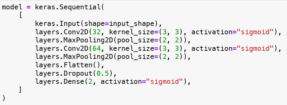
Figure 1: CNN model with sigmoid activations

A Proof of Lemma 4

Observe that

$$\psi(x) =ReLU(\mathbf{x})-\alpha ReLU(-x)$$ (155)

$$=\frac{x+|x|}{2}-\alpha\frac{-x+|x|}{2}$$ (156)

$$=\frac{1+\alpha}{2}x+\frac{(1-\alpha)}{2}|x|.$$ (157)

Then, for any $p\geq 1$ we have

$$\frac{1}{n}\mathbb{E}_{\bm{\varepsilon}}\bigg{[}\sup_{h\in\mathcal{H}}\bigg{\|}\sum_{i=1}^{n}\varepsilon_{i}\psi(h(\mathbf{x}_{i}))\bigg{\|}_{p}\bigg{]}$$ (158)

$$\qquad\leq\bigg{(}\frac{1+\alpha}{2}\bigg{)}\frac{1}{n}\mathbb{E}_{\bm{\varepsilon}}\bigg{[}\sup_{h\in\mathcal{H}}\bigg{\|}\sum_{i=1}^{n}\varepsilon_{i}[h(\mathbf{x}_{i})]\bigg{\|}_{p}\bigg{]}$$

$$\qquad\qquad+\bigg{(}\frac{1-\alpha}{2}\bigg{)}\frac{1}{n}\mathbb{E}_{\bm{\varepsilon}}\bigg{[}\sup_{h\in\mathcal{H}}\bigg{\|}\sum_{i=1}^{n}\varepsilon_{i}\big{|}[h(\mathbf{x}_{i})]\big{|}\bigg{\|}_{p}\bigg{]}$$ (159)

$$\qquad=\frac{1}{n}\mathbb{E}_{\bm{\varepsilon}}\bigg{[}\sup_{h\in\mathcal{H}_{+}}\bigg{\|}\sum_{i=1}^{n}\varepsilon_{i}[h(\mathbf{x}_{i})]\bigg{\|}_{p}\bigg{]},$$ (160)

where (159) follows from Minkowski’s inequality Royden and Fitzpatrick (2010), and (160) follows from the fact that $|h|\in\mathcal{H}_{+}$ if $h\in\mathcal{H}$.

B Proof of Lemma 6

First, we have

$$\mathbb{E}_{\bm{\varepsilon}}\bigg{[}\sup_{h\in\mathcal{H}}\bigg{\|}\frac{1}{n}\sum_{i=1}^{n}\varepsilon_{i}\psi(h(\mathbf{x}_{i}))\bigg{\|}_{\infty}\bigg{]}$$

$$\qquad\leq\frac{1}{n}\bigg{(}\mathbb{E}_{\bm{\varepsilon}}\bigg{[}\sup_{h\in\mathcal{H}}\bigg{\|}\sum_{i=1}^{n}\varepsilon_{i}\bigg{(}\psi(h(\mathbf{x}_{i}))-\psi(\b{0})\bigg{)}\bigg{\|}_{\infty}\bigg{]}+\mathbb{E}_{\bm{\varepsilon}}\bigg{[}\sup_{h\in\mathcal{H}}\bigg{\|}\sum_{i=1}^{n}\varepsilon_{i}\psi(\b{0})\bigg{\|}_{\infty}\bigg{]}\bigg{)}$$ (161)

$$\qquad\leq\frac{1}{n}\bigg{(}\mathbb{E}_{\bm{\varepsilon}}\bigg{[}\sup_{h\in\mathcal{H}}\bigg{\|}\sum_{i=1}^{n}\varepsilon_{i}\bigg{(}\psi(h(\mathbf{x}_{i}))-\psi(\b{0})\bigg{)}\bigg{\|}_{\infty}\bigg{]}+\mathbb{E}_{\bm{\varepsilon}}\bigg{[}\bigg{\|}\sum_{i=1}^{n}\varepsilon_{i}\psi(\b{0})\bigg{\|}_{\infty}\bigg{]}\bigg{)}$$ (162)

$$\qquad\leq\frac{1}{n}\bigg{(}\mathbb{E}_{\bm{\varepsilon}}\bigg{[}\sup_{h\in\mathcal{H}}\bigg{\|}\sum_{i=1}^{n}\varepsilon_{i}\bigg{(}\psi(h(\mathbf{x}_{i}))-\psi(\b{0})\bigg{)}\bigg{\|}_{\infty}\bigg{]}+\sup_{j\in[m]}\sqrt{\mathbb{E}_{\bm{\varepsilon}}\bigg{[}\bigg{(}\sum_{i=1}^{n}\varepsilon_{i}\psi_{j}(\b{0})\bigg{)}^{2}}\bigg{]}\bigg{)}$$ (163)

$$\qquad\leq\frac{1}{n}\mathbb{E}_{\bm{\varepsilon}}\bigg{[}\sup_{h\in\mathcal{H}}\bigg{\|}\sum_{i=1}^{n}\varepsilon_{i}\bigg{(}\psi(h(\mathbf{x}_{i}))-\psi(\b{0})\bigg{)}\bigg{\|}_{\infty}\bigg{]}+\sup_{j\in[m]}\big{|}\psi_{j}(\b{0})\big{|}\frac{1}{\sqrt{n}},$$ (164)

where (161) follows from the triangular property of the $\infty$-norm Royden and Fitzpatrick (2010), and (163) follows from Cauchy-Schwarz inequality and the assumption that $\psi_{j}(\b{0})$ does not depend on $j$.

Define $\tilde{\psi}(\mathbf{x}):=\psi(\mathbf{x})-\psi(\b{0})$ for all $\mathbf{x}\in\mathbb{R}^{m}$. Then, we have $\tilde{\psi}(\b{0})=\b{0}$, and $\tilde{\psi}$ is also $\mu$-Lipschitz. In addition, by our assumption, $\tilde{\psi}$ is odd.

Let

$$\Psi=\big{\{}\tilde{\psi}:\mathbb{R}^{m}\to\mathbb{R}^{m},\mbox{st.}\enspace\tilde{\psi}(-\mathbf{x})=-\tilde{\psi}(\mathbf{x}),|\tilde{\psi}_{j}(\mathbf{x})-\tilde{\psi}(\mathbf{y})|\leq\mu|x_{j}-y_{j}|\enspace\forall\mathbf{x},\mathbf{y}\in\mathbb{R}^{m},j\in[m]\big{\}}.$$ (165)

It follows that

$$\mathbb{E}_{\bm{\varepsilon}}\bigg{[}\sup_{h\in\mathcal{H}}\bigg{\|}\frac{1}{n}\sum_{i=1}^{n}\varepsilon_{i}\tilde{\psi}\big{(}h(\mathbf{x}_{i})\big{)}\bigg{\|}_{\infty}\bigg{]}$$ (166)

$$\qquad=\frac{1}{n}\mathbb{E}_{\bm{\varepsilon}}\bigg{[}\sup_{j\in[m]}\sup_{h\in\mathcal{H}}\bigg{|}\sum_{i=1}^{n}\varepsilon_{i}\tilde{\psi}_{j}\big{(}h(\mathbf{x}_{i})\big{)}\bigg{|}\bigg{]}$$ (167)

$$\qquad\leq\frac{1}{n}\mathbb{E}_{\bm{\varepsilon}}\bigg{[}\sup_{s\in\{-1,+1\}^{m}}\sup_{j\in[m]}\sup_{h\in\mathcal{H}}s_{j}\bigg{(}\sum_{i=1}^{n}\varepsilon_{i}\tilde{\psi}_{j}\big{(}h(\mathbf{x}_{i})\big{)}\bigg{)}\bigg{]}$$ (168)

$$\qquad=\frac{1}{n}\mathbb{E}_{\bm{\varepsilon}}\bigg{[}\sup_{s\in\{-1,+1\}^{m}}\sup_{j\in[m]}\sup_{h\in\mathcal{H}}\sum_{i=1}^{n}\varepsilon_{i}s_{j}\tilde{\psi}_{j}\big{(}h(\mathbf{x}_{i})\big{)}\bigg{]}$$ (169)

$$\qquad=\frac{1}{n}\mathbb{E}_{\bm{\varepsilon}}\bigg{[}\sup_{s\in\{-1,+1\}^{m}}\sup_{j\in[m]}\sup_{h\in\mathcal{H}}\sum_{i=1}^{n}\varepsilon_{i}\tilde{\psi}_{j}^{(\mathbf{s})}\big{(}h(\mathbf{x}_{i})\big{)}\bigg{]}$$ (170)

$$\qquad\leq\frac{1}{n}\mathbb{E}_{\bm{\varepsilon}}\bigg{[}\sup_{\tilde{\psi}\in\Psi}\sup_{s\in\{-1,+1\}^{m}}\sup_{j\in[m]}\sup_{h\in\mathcal{H}}\sum_{i=1}^{n}\varepsilon_{i}\tilde{\psi}_{j}\big{(}h(\mathbf{x}_{i})\big{)}\bigg{]}$$ (171)

$$\qquad\leq\frac{1}{n}\mathbb{E}_{\bm{\varepsilon}}\bigg{[}\sup_{\tilde{\psi}\in\Psi}\sup_{j\in[m]}\sup_{h\in\mathcal{H}_{+}}\sum_{i=1}^{n}\varepsilon_{i}\tilde{\psi}_{j}\big{(}h(\mathbf{x}_{i})\big{)}\bigg{]},$$ (172)

where (170) follows by defining $\tilde{\psi}^{(\mathbf{s})}=(s_{1}\tilde{\psi}_{1},s_{2}\tilde{\psi}_{2},\cdots,s_{m}\tilde{\psi}_{m})$ for any $\mathbf{s}\in\{-1,+1\}^{m}$, (171) follows from the fact that $\tilde{\psi}^{(\mathbf{s})}\in\Psi$ for any fixed $\mathbf{s}$, and (172) follows from the definition of $\mathcal{H}_{+}$.

Now, we have

$$\mathbb{E}_{\bm{\varepsilon}}\bigg{[}\sup_{\tilde{\psi}\in\Psi}\sup_{j\in[m]}\sup_{h\in\mathcal{H}_{+}}\sum_{i=1}^{n}\varepsilon_{i}\tilde{\psi}_{j}\big{(}h(\mathbf{x}_{i})\big{)}\bigg{]}$$

$$\qquad=\mathbb{E}_{\varepsilon_{1},\varepsilon_{2},\cdots,\varepsilon_{n-1}}\bigg{[}\mathbb{E}_{\varepsilon_{n}}\bigg{[}\sup_{\tilde{\psi}\in\Psi}\sup_{j\in[m]}\sup_{h\in\mathcal{H}_{+}}u_{n-1}(h,j)+\varepsilon_{n}\tilde{\psi}_{j}\big{(}h(\mathbf{x}_{n})\big{)}\bigg{]}\bigg{]},$$ (173)

where

$$u_{n-1}(h,j):=\sum_{i=1}^{n-1}\varepsilon_{i}\tilde{\psi}_{j}\big{(}h(\mathbf{x}_{i})\big{)}.$$ (174)

Since $\varepsilon_{n}$ is uniformly distributed over $\{-1,1\}$, we have

$$\mathbb{E}_{\varepsilon_{n}}\bigg{[}\sup_{\tilde{\psi}\in\Psi}\sup_{j\in[m]}\sup_{h\in\mathcal{H}_{+}}u_{n-1}(h,j)+\varepsilon_{n}\tilde{\psi}_{j}\big{(}h(\mathbf{x}_{n})\big{)}\bigg{]}$$

$$\qquad=\frac{1}{2}\bigg{(}\sup_{\tilde{\psi}\in\Psi}\sup_{j\in[m]}\sup_{h\in\mathcal{H}_{+}}u_{n-1}(h,j)+\tilde{\psi}_{j}(h(\mathbf{x}_{n}))\bigg{)}$$

$$\qquad\qquad+\frac{1}{2}\bigg{(}\sup_{\tilde{\psi}\in\Psi}\sup_{j\in[m]}\sup_{h\in\mathcal{H}_{+}}u_{n-1}(h,j)-\tilde{\psi}_{j}(h(\mathbf{x}_{n}))\bigg{)}.$$ (175)

Hence, we have

$$\mathbb{E}_{\bm{\varepsilon}}\bigg{[}\sup_{\tilde{\psi}\in\Psi}\sup_{j\in[m]}\sup_{h\in\mathcal{H}_{+}}\sum_{i=1}^{n}\varepsilon_{i}\tilde{\psi}_{j}\big{(}h(\mathbf{x}_{i})\big{)}\bigg{]}$$

$$\qquad=\frac{1}{2}\mathbb{E}_{\varepsilon_{1},\varepsilon_{2},\cdots,\varepsilon_{n-1}}\bigg{[}\sup_{\tilde{\psi}\in\Psi}\sup_{j\in[m]}\sup_{h\in\mathcal{H}_{+}}u_{n-1}(h,j)+\tilde{\psi}_{j}(h(\mathbf{x}_{n}))\bigg{]}$$

$$\qquad\qquad+\frac{1}{2}\mathbb{E}_{\varepsilon_{1},\varepsilon_{2},\cdots,\varepsilon_{n-1}}\bigg{[}\sup_{\tilde{\psi}\in\Psi}\sup_{j\in[m]}\sup_{h\in\mathcal{H}_{+}}u_{n-1}(h,j)-\tilde{\psi}_{j}(h(\mathbf{x}_{n}))\bigg{]}$$ (176)

$$\qquad=\frac{1}{2}\mathbb{E}_{\varepsilon_{1},\varepsilon_{2},\cdots,\varepsilon_{n-1}}\bigg{[}\sup_{\tilde{\psi}\in\Psi}\sup_{j\in[m]}\sup_{h\in\mathcal{H}_{+}}u_{n-1}(h,j)+\tilde{\psi}_{j}(h(\mathbf{x}_{n}))\bigg{]}$$

$$\qquad\qquad+\frac{1}{2}\mathbb{E}_{\varepsilon_{1},\varepsilon_{2},\cdots,\varepsilon_{n-1}}\bigg{[}\sup_{\tilde{\psi}\in\Psi}\sup_{j\in[m]}\sup_{h\in\mathcal{H}_{+}}-u_{n-1}(h,j)-\tilde{\psi}_{j}(h(\mathbf{x}_{n}))\bigg{]}$$ (177)

$$\qquad=\mathbb{E}_{\varepsilon_{1},\varepsilon_{2},\cdots,\varepsilon_{n-1}}\bigg{[}\frac{1}{2}\bigg{(}\sup_{\tilde{\psi}\in\Psi}\sup_{j\in[m]}\sup_{h\in\mathcal{H}_{+}}u_{n-1}(h,j)+\tilde{\psi}_{j}(h(\mathbf{x}_{n}))\bigg{)}$$

$$\qquad\qquad+\frac{1}{2}\bigg{(}\sup_{\tilde{\psi}\in\Psi}\sup_{j\in[m]}\sup_{h\in\mathcal{H}_{+}}-u_{n-1}(h,j)-\tilde{\psi}_{j}(h(\mathbf{x}_{n}))\bigg{)}\bigg{]},$$ (178)

where (177) follows from the fact that $(-\varepsilon_{1},-\varepsilon_{2},\cdots,-\varepsilon_{n-1})$ is a tuple of independent Rademacher random variables which has the same distribution as $(\varepsilon_{1},\varepsilon_{2},\cdots,\varepsilon_{n-1})$.

Now, given any $j\in[m]$ and $\tilde{\psi}\in\Psi$ we have

$$\sup_{h\in\mathcal{H}_{+}}u_{n-1}(h,j)+\tilde{\psi}_{j}(h(\mathbf{x}_{n}))$$

$$\qquad=\sup_{h\in\mathcal{H}_{+}}u_{n-1}(-h,j)+\tilde{\psi}_{j}(-h(\mathbf{x}_{n}))$$ (179)

$$\qquad=\sup_{h\in\mathcal{H}_{+}}-u_{n-1}(h,j)-\tilde{\psi}_{j}(h(\mathbf{x}_{n})),$$ (180)

where (179) follows from the assumption that $h\in\mathcal{H}_{+}$ if and only if $-h\in\mathcal{H}_{+}$, and (180) follows from the assumption that $\tilde{\psi}$ is odd for any $\tilde{\psi}\in\Psi$.

Hence, for any arbitrarily small $\delta>0$ there exists $j_{0}\in[m],\tilde{\psi}_{0}\in\Psi$ and $h_{1},h_{2}\in\mathcal{H}$ such that

$$\sup_{j\in[m]}\sup_{h\in\mathcal{H}_{+}}u_{n-1}(h,j)+\tilde{\psi}_{j}(h(\mathbf{x}_{n}))\leq u_{n-1}(h_{1},j_{0})+\tilde{\psi}_{0,j_{0}}(h_{1}(\mathbf{x}_{n}))+\delta,$$ (181)

and

$$\sup_{j\in[m]}\sup_{h\in\mathcal{H}_{+}}-u_{n-1}(h,j)-\tilde{\psi}([h(\mathbf{x}_{n})]_{j})\leq-u_{n-1}(h_{2},j_{0})-\tilde{\psi}_{0,j_{0}}(h_{2}(\mathbf{x}_{n}))+\delta.$$ (182)

It follows that

$$\frac{1}{2}\bigg{(}\sup_{\tilde{\psi}\in\Psi}\sup_{j\in[m]}\sup_{h\in\mathcal{H}_{+}}u_{n-1}(h,j)+\tilde{\psi}_{j}(h(\mathbf{x}_{n}))\bigg{)}$$

$$\qquad\qquad+\frac{1}{2}\bigg{(}\sup_{\tilde{\psi}\in\Psi}\sup_{j\in[m]}\sup_{h\in\mathcal{H}_{+}}-u_{n-1}(h,j)-\tilde{\psi}_{j}(h(\mathbf{x}_{n}))\bigg{)}$$

$$\qquad\leq\frac{1}{2}\bigg{(}u_{n-1}(h_{1},j_{0})+\tilde{\psi}_{0,j_{0}}(h_{1}(\mathbf{x}_{n}))\bigg{)}$$

$$\qquad\qquad+\frac{1}{2}\bigg{(}-u_{n-1}(h_{2},j_{0})-\tilde{\psi}_{0,j_{0}}(h_{2}(\mathbf{x}_{n}))\bigg{)}+\delta$$ (183)

$$\qquad=\frac{1}{2}\big{(}u_{n-1}(h_{1},j_{0})-u_{n-1}(h_{2},j_{0})\big{)}$$

$$\qquad\qquad+\frac{1}{2}\big{(}\tilde{\psi}_{0,j_{0}}(h_{1}(\mathbf{x}_{n}))-\tilde{\psi}_{0,j_{0}}(h_{2}(\mathbf{x}_{n}))\big{)}+\delta$$ (184)

$$\qquad\leq\frac{1}{2}\big{(}u_{n-1}(h_{1},j_{0})-u_{n-1}(h_{2},j_{0})\big{)}+\frac{\mu}{2}\big{|}[h_{1}(\mathbf{x}_{n})]_{j_{0}}-[h_{2}(\mathbf{x}_{n})]_{j_{0}}\big{|}$$ (185)

$$\qquad=\frac{1}{2}\big{(}u_{n-1}(h_{1},j_{0})-u_{n-1}(h_{2},j_{0})\big{)}+\frac{\mu}{2}s_{12,n}\big{(}[h_{1}(\mathbf{x}_{n})]_{j_{0}}-[h_{2}(\mathbf{x}_{n})]_{j_{0}}\big{)}$$ (186)

$$\qquad=\frac{1}{2}\big{(}u_{n-1}(h_{1},j_{0})+\mu s_{12,n}[h_{1}(\mathbf{x}_{n})]_{j_{0}}\big{)}+\frac{1}{2}\big{(}-u_{n-1}(h_{2},j_{0})-\mu s_{12,n}[h_{2}(\mathbf{x}_{n})]_{j_{0}}\big{)}$$ (187)

$$\qquad\leq\sup_{s_{12}\in\{-1,+1\}}\frac{1}{2}\big{(}u_{n-1}(h_{1},j_{0})+\mu s_{12}[h_{1}(\mathbf{x}_{n})]_{j_{0}}\big{)}+\frac{1}{2}\big{(}-u_{n-1}(h_{2},j_{0})-\mu s_{12}[h_{2}(\mathbf{x}_{n})]_{j_{0}}\big{)}$$ (188)

$$\qquad\leq\sup_{s_{12}\in\{-1,+1\}}\frac{1}{2}\sup_{\tilde{\psi}\in\Psi}\sup_{j\in[m]}\sup_{h\in\mathcal{H}_{+}}u_{n-1}(h,j)+\mu s_{12}[h(\mathbf{x}_{n})]_{j}$$

$$\qquad\qquad+\frac{1}{2}\sup_{\tilde{\psi}\in\Psi}\sup_{j\in[m]}\sup_{h\in\mathcal{H}_{+}}-u_{n-1}(h,j)-\mu s_{12}[h(\mathbf{x}_{n})]_{j}$$ (189)

$$\qquad\leq\sup_{s_{12}\in\{-1,+1\}}\frac{1}{2}\sup_{\tilde{\psi}\in\Psi}\sup_{j\in[m]}\sup_{h\in\mathcal{H}_{+}}u_{n-1}(h,j)+\mu s_{12}[h(\mathbf{x}_{n})]_{j}$$

$$\qquad\qquad+\frac{1}{2}\sup_{\tilde{\psi}\in\Psi}\sup_{j\in[m]}\sup_{h\in\mathcal{H}_{+}}u_{n-1}(h,j)-\mu s_{12}[h(\mathbf{x}_{n})]_{j},$$ (190)

where $s_{12,n}:=\operatorname{sgn}\big{(}[h_{1}(\mathbf{x}_{n})]_{j_{0}}-[h_{2}(\mathbf{x}_{n})]_{j_{0}}\big{)}$ in (186), and (190) follows from the fact that $-\tilde{\psi}\in\Psi$ if $\tilde{\psi}\in\Psi$.

From (190) we obtain

$$\frac{1}{2}\bigg{(}\sup_{\tilde{\psi}\in\Psi}\sup_{j\in[m]}\sup_{h\in\mathcal{H}_{+}}u_{n-1}(h,j)+\tilde{\psi}_{j}(h(\mathbf{x}_{n}))\bigg{)}$$

$$\qquad\qquad+\frac{1}{2}\bigg{(}\sup_{\tilde{\psi}\in\Psi}\sup_{j\in[m]}\sup_{h\in\mathcal{H}_{+}}-u_{n-1}(h,j)-\tilde{\psi}_{j}(h(\mathbf{x}_{n}))\bigg{)}$$ (191)

$$\qquad\leq\sup_{s_{12}\in\{-1,+1\}}\mathbb{E}_{\tilde{\varepsilon}_{n}}\bigg{[}\sup_{\tilde{\psi}\in\Psi}\sup_{j\in[m]}\sup_{h\in\mathcal{H}_{+}}u_{n-1}(h,j)+\mu\tilde{\varepsilon}_{n}s_{12}[h(\mathbf{x}_{n})]_{j}\bigg{]}$$ (192)

for some Rademacher random variable $\tilde{\varepsilon}_{n}$ which is independent of $(\varepsilon_{1},\varepsilon_{2},\cdots,\varepsilon_{n-1})$.

Since $\tilde{\varepsilon}_{n}s_{12}\sim\tilde{\varepsilon}_{n}$ for any fixed $s_{12}\in\{-1,+1\}$, from (192) we have

$$\frac{1}{2}\bigg{(}\sup_{\tilde{\psi}\in\Psi}\sup_{j\in[m]}\sup_{h\in\mathcal{H}_{+}}u_{n-1}(h,j)+\tilde{\psi}_{j}(h(\mathbf{x}_{n}))\bigg{)}$$

$$\qquad\qquad+\frac{1}{2}\bigg{(}\sup_{\tilde{\psi}\in\Psi}\sup_{j\in[m]}\sup_{h\in\mathcal{H}_{+}}-u_{n-1}(h,j)-\tilde{\psi}_{j}(h(\mathbf{x}_{n}))\bigg{)}$$ (193)

$$\qquad\leq\mathbb{E}_{\tilde{\varepsilon}_{n}}\bigg{[}\sup_{\tilde{\psi}\in\Psi}\sup_{j\in[m]}\sup_{h\in\mathcal{H}_{+}}u_{n-1}(h,j)+\mu\tilde{\varepsilon}_{n}[h(\mathbf{x}_{n})]_{j}\bigg{]}.$$ (194)

From (178) and (194) we obtain

$$\mathbb{E}_{\bm{\varepsilon}}\bigg{[}\sup_{\tilde{\psi}\in\Psi}\sup_{j\in[m]}\sup_{h\in\mathcal{H}_{+}}\sum_{i=1}^{n}\varepsilon_{i}\tilde{\psi}_{j}\big{(}h(\mathbf{x}_{i})\big{)}\bigg{]}$$

$$\qquad\leq\mathbb{E}_{\varepsilon_{1},\varepsilon_{2},\cdots,\varepsilon_{n-1}}\bigg{[}\mathbb{E}_{\tilde{\varepsilon}_{n}}\bigg{[}\sup_{\tilde{\psi}\in\Psi}\sup_{j\in[m]}\sup_{h\in\mathcal{H}_{+}}u_{n-1}(h,j)+\mu\tilde{\varepsilon}_{n}[h(\mathbf{x}_{n})]_{j}\bigg{]}\bigg{]}$$ (195)

$$\qquad=\mathbb{E}_{\tilde{\varepsilon}_{n}}\bigg{[}\mathbb{E}_{\varepsilon_{1},\varepsilon_{2},\cdots,\varepsilon_{n-1}}\bigg{[}\sup_{\tilde{\psi}\in\Psi}\sup_{j\in[m]}\sup_{h\in\mathcal{H}_{+}}u_{n-1}(h,j)+\mu\tilde{\varepsilon}_{n}[h(\mathbf{x}_{n})]_{j}\bigg{]}\bigg{]}.$$ (196)

By continuing this process (peeling) for $n-1$ more times, we have

$$\mathbb{E}_{\bm{\varepsilon}}\bigg{[}\sup_{\tilde{\psi}\in\Psi}\sup_{j\in[m]}\sup_{h\in\mathcal{H}_{+}}u_{n-1}(h,j)+\tilde{\varepsilon}_{n}\mu[h(\mathbf{x}_{n})]_{j}\bigg{]}$$

$$\qquad\leq\mu\mathbb{E}_{\tilde{\varepsilon}_{1},\tilde{\varepsilon}_{2},\cdots,\tilde{\varepsilon}_{n}}\bigg{[}\sup_{j\in[m]}\sup_{h\in\mathcal{H}_{+}}\sum_{i=1}^{n}\tilde{\varepsilon}_{i}[h(\mathbf{x}_{n})]_{j}\bigg{]}$$ (197)

$$\qquad=\mu\mathbb{E}_{\bm{\varepsilon}}\bigg{[}\sup_{j\in[m]}\sup_{h\in\mathcal{H}_{+}}\sum_{i=1}^{n}\varepsilon_{i}[h(\mathbf{x}_{n})]_{j}\bigg{]}$$ (198)

$$\qquad\leq\mu\mathbb{E}_{\bm{\varepsilon}}\bigg{[}\sup_{j\in[m]}\sup_{h\in\mathcal{H}_{+}}\bigg{|}\sum_{i=1}^{n}\varepsilon_{i}[h(\mathbf{x}_{n})]_{j}\bigg{|}\bigg{]}$$ (199)

$$\qquad=\mu\mathbb{E}_{\bm{\varepsilon}}\bigg{[}\sup_{h\in\mathcal{H}_{+}}\bigg{\|}\sum_{i=1}^{n}\varepsilon_{i}h(\mathbf{x}_{n})\bigg{\|}_{\infty}\bigg{]}.$$ (200)

From (164) and (200), we obtain

$$\mathbb{E}_{\bm{\varepsilon}}\bigg{[}\sup_{h\in\mathcal{H}}\bigg{\|}\frac{1}{n}\sum_{i=1}^{n}\varepsilon_{i}\psi(h(\mathbf{x}_{i}))\bigg{\|}_{\infty}\bigg{]}$$

$$\qquad\leq\mu\mathbb{E}_{\bm{\varepsilon}}\bigg{[}\sup_{h\in\mathcal{H}_{+}}\bigg{\|}\frac{1}{n}\sum_{i=1}^{n}\varepsilon_{i}h(\mathbf{x}_{n})\bigg{\|}_{\infty}\bigg{]}+\sup_{j\in[m]}\big{|}\psi_{j}(0)\big{|}\frac{1}{\sqrt{n}}.$$ (201)

This concludes our proof of Lemma 6.

C Proof of Lemma 12

Let

$$\mathbf{1}_{\tau_{l}^{2}} =\underbrace{\begin{bmatrix}1&1&\cdots&1\end{bmatrix}}_{\tau_{l}^{2}},$$ (202)

$$0_{\tau_{l}^{2}} =\underbrace{\begin{bmatrix}0&0&\cdots&0\end{bmatrix}}_{\tau_{l}^{2}},$$ (203)

and

$$\mathbf{A}=\frac{1}{\tau_{l}^{2}}\begin{bmatrix}\mathbf{1}_{\tau_{l}^{2}}&0_{\tau_{l}^{2}}&0_{\tau_{l}^{2}}&\cdots&0_{\tau_{l}^{2}}&0_{\tau_{l}^{2}}\\ 0_{\tau_{l}^{2}}&\mathbf{1}_{\tau_{l}^{2}}&0_{\tau_{l}^{2}}&\cdots&0_{\tau_{l}^{2}}&0_{\tau_{l}^{2}}\\ \vdots&\vdots&\vdots&\ddots&\vdots&\vdots\\ 0_{\tau_{l}^{2}}&0_{\tau_{l}^{2}}&0_{\tau_{l}^{2}}&\cdots&0_{\tau_{l}^{2}}&\mathbf{1}_{\tau_{l}^{2}}\end{bmatrix}\in\mathbb{R}^{\lceil(d-r_{l}+1)^{2}/\tau_{l}^{2}\rceil\tau_{l}^{2}\times\lceil(d-r_{l}+1)^{2}/\tau_{l}^{2}\rceil\tau_{l}^{2}}.$$ (204)

Then, for all $\mathbf{x}\in\mathbb{R}^{d^{2}}$ and $l\in[Q]$, we have

$$\psi_{l}(\mathbf{x})=\sigma_{\rm{avg}}\circ\sigma_{l}(\mathbf{x}),$$ (205)

where

$$\sigma_{\rm{avg}}(\mathbf{x})=\mathbf{A}\mathbf{x},\qquad\forall\mathbf{x}\in\mathbb{R}^{\lceil(d-r_{l}+1)^{2}/\tau_{l}^{2}\rceil\tau_{l}^{2}}.$$ (206)

Now, for all $\mathbf{x},\mathbf{y}\in\mathbb{R}^{\lceil(d-r_{l}+1)^{2}/\tau_{l}^{2}\rceil\tau_{l}^{2}}$ we have

$$\big{\|}\sigma_{\rm{avg}}(\mathbf{x})-\sigma_{\rm{avg}}(\mathbf{y})\big{\|}_{\infty}$$

$$\qquad\leq\frac{1}{\tau_{l}^{2}}\max_{j\in[\lceil(d-r_{l}+1)^{2}/\tau_{l}^{2}\rceil]}\sum_{k=(j-1)\tau_{l}^{2}+1}^{j\tau_{l}^{2}}\big{|}x_{k}-y_{k}\big{|}$$ (207)

$$\qquad\leq\big{\|}\mathbf{x}-\mathbf{y}\big{\|}_{\infty}.$$ (208)

Hence, we have

$$\|\mathbf{A}\|_{\infty}\leq 1.$$ (209)

Hence, by Lemma 3 we have

$$\mathbb{E}\bigg{[}\sup_{l\in[Q]}\sup_{\psi_{l}\in\Psi}\sup_{f\in\mathcal{F}}\bigg{\|}\frac{1}{n}\sum_{i=1}^{n}\varepsilon_{i}\psi_{l}\circ f(\mathbf{x}_{i})\bigg{\|}_{\infty}\bigg{]}$$

$$\qquad=\mathbb{E}\bigg{[}\sup_{l\in[Q]}\sup_{\sigma_{\rm{avg}}}\sup_{\sigma_{l}}\sup_{f\in\mathcal{F}}\bigg{\|}\frac{1}{n}\sum_{i=1}^{n}\varepsilon_{i}\sigma_{\rm{avg}}\circ\sigma_{l}\circ f(\mathbf{x}_{i})\bigg{\|}_{\infty}\bigg{]}$$ (210)

$$\qquad\leq\mathbb{E}\bigg{[}\sup_{l\in[Q]}\sup_{\sigma_{l}}\sup_{f\in\mathcal{F}}\bigg{\|}\frac{1}{n}\sum_{i=1}^{n}\varepsilon_{i}\sigma_{l}\circ f(\mathbf{x}_{i})\bigg{\|}_{\infty}\bigg{]}.$$ (211)

In addition, for all $\mathbf{x}\in\mathbb{R}^{d\times d}$,

$$\sigma_{l}(\mathbf{x}) =\{\sigma(\hat{x}(a,b))\}_{a,b=1}^{d-r_{l}+1},$$ (212)

$$\hat{x}(a,b) =\sum_{u=0}^{r_{l}-1}\sum_{v=0}^{r_{l}-1}x(a+u,b+v)W_{l}(u+1,v+1).$$ (213)

Hence, we have

$$\big{\|}\sigma_{l}(\mathbf{x})-\sigma_{l}(\mathbf{y})\big{\|}_{\infty}$$

$$\qquad\leq\mu\max_{a\in[d-r_{l}+1]}\max_{b\in[d-r_{l}+1]}\sum_{u=0}^{r_{l}-1}\sum_{v=0}^{r_{l}-1}\big{|}W_{l}(u+1,v+1)x(a+u,b+v)$$

$$\qquad\qquad\qquad-W_{l}(u+1,v+1)y(a+u,b+v)\big{|}$$ (214)

$$\qquad\leq\mu\sum_{u=0}^{r_{l}-1}\sum_{v=0}^{r_{l}-1}\big{|}W_{l}(u+1,v+1)\big{|}\|\mathbf{x}-\mathbf{y}\|_{\infty}.$$ (215)

Since the convolution is linear, it is also easy to see that $\sigma_{l}$ is the composition of a linear map and a point-wise activation map. Hence, by Lemma 3 and Theorem 9 we have

$$\mathbb{E}\bigg{[}\sup_{l\in[Q]}\sup_{\sigma_{l}}\sup_{f\in\mathcal{F}}\bigg{\|}\frac{1}{n}\sum_{i=1}^{n}\varepsilon_{i}\sigma_{l}\circ f(\mathbf{x}_{i})\bigg{\|}_{\infty}\bigg{]}$$

$$\qquad\qquad\leq\bigg{[}\gamma(\mu)\bigg{(}\sum_{u=0}^{r_{l}-1}\sum_{v=0}^{r_{l}-1}\big{|}W_{l}(u+1,v+1)\big{|}\bigg{)}+\frac{|\sigma(0)|}{\sqrt{n}}\bigg{]}\mathbb{E}\bigg{[}\sup_{f\in\mathcal{F}_{+}}\bigg{\|}\frac{1}{n}\sum_{i=1}^{n}\varepsilon_{i}f(\mathbf{x}_{i})\bigg{\|}_{\infty}\bigg{]}.$$ (216)

Finally, from (211) and (216) we obtain

$$\mathbb{E}\bigg{[}\sup_{l\in[Q]}\sup_{\psi_{l}\in\Psi}\sup_{f\in\mathcal{F}}\bigg{\|}\frac{1}{n}\sum_{i=1}^{n}\varepsilon_{i}\psi_{l}\circ f(\mathbf{x}_{i})\bigg{\|}_{\infty}\bigg{]}$$

$$\qquad\leq\bigg{[}\gamma(\mu)\bigg{(}\sum_{u=0}^{r_{l}-1}\sum_{v=0}^{r_{l}-1}\big{|}W_{l}(u+1,v+1)\big{|}\bigg{)}+\frac{|\sigma(0)|}{\sqrt{n}}\bigg{]}\mathbb{E}\bigg{[}\sup_{f\in\mathcal{F}_{+}}\bigg{\|}\frac{1}{n}\sum_{i=1}^{n}\varepsilon_{i}f(\mathbf{x}_{i})\bigg{\|}_{\infty}\bigg{]}.$$ (217)

D Proof of Lemma 13

Let

$$e_{\tau_{l}^{2}} =\underbrace{\begin{bmatrix}1&0&\cdots&0\end{bmatrix}}_{\tau_{l}^{2}},$$ (218)

$$0_{\tau_{l}^{2}} =\underbrace{\begin{bmatrix}0&0&\cdots&0\end{bmatrix}}_{\tau_{l}^{2}},$$ (219)

and

$$\mathbf{B}=\begin{bmatrix}e_{\tau_{l}^{2}}&0_{\tau_{l}^{2}}&0_{\tau_{l}^{2}}&\cdots&0_{\tau_{l}^{2}}&0_{\tau_{l}^{2}}\\ 0_{\tau_{l}^{2}}&e_{\tau_{l}^{2}}&0_{\tau_{l}^{2}}&\cdots&0_{\tau_{l}^{2}}&0_{\tau_{l}^{2}}\\ \vdots&\vdots&\vdots&\ddots&\vdots&\vdots\\ 0_{\tau_{l}^{2}}&0_{\tau_{l}^{2}}&0_{\tau_{l}^{2}}&\cdots&0_{\tau_{l}^{2}}&e_{\tau_{l}^{2}}\end{bmatrix}\in\mathbb{R}^{\lceil(d-r_{l}+1)^{2}/\tau_{l}^{2}\rceil\tau_{l}^{2}\times\lceil(d-r_{l}+1)^{2}/\tau_{l}^{2}\rceil\tau_{l}^{2}}.$$ (220)

For all $\mathbf{x}\in\mathbb{R}^{d^{2}}$ and $l\in[Q]$, observe that

$$\psi_{l}(\mathbf{x})=\sigma_{\rm{max}}\circ\sigma_{l}(\mathbf{x}),$$ (221)

where

$$\sigma_{\rm{max}}(\mathbf{x}) =\bigg{(}\max_{k\in[\tau_{l}^{2}]}x_{k},\cdots\max_{k\in[(j-1)\tau_{l}^{2}+1,j\tau_{l}^{2}]}x_{k},$$

$$\qquad\cdots,\max_{k\in[\lceil(d-r_{l}+1)^{2}/\tau_{l}^{2}\rceil-r_{l}^{2}+1,\lceil(d-r_{l}+1)^{2}/\tau_{l}^{2}\rceil\tau_{l}^{2}]}x_{k}\bigg{)},$$

$$\qquad\qquad\qquad\forall\mathbf{x}\in\mathbb{R}^{\lceil(d-r_{l}+1)^{2}/\tau_{l}^{2}\rceil\tau_{l}^{2}},$$ (222)

and for all $\mathbf{x}\in\mathbb{R}^{d\times d}$,

$$\sigma_{l}(\mathbf{x}) =\{\hat{x}(a,b)\}_{a,b=1}^{d-r_{l}+1},$$ (223)

$$\hat{x}(a,b) =\sum_{u=0}^{r_{l}-1}\sum_{v=0}^{r_{l}-1}x(a+u,b+v)W_{l}(u+1,v+1).$$ (224)

Now, let $\pi_{\tau_{l}^{2}}(\mathbf{x})$ is a non-increasing order of $\mathbf{x}$ for all $\mathbf{x}\in\mathbb{R}^{\tau_{l}^{2}}$. Then, $\sigma_{\max}$ can be written as

$$\sigma_{\max}(\mathbf{x})=\mathbf{B}\hat{\sigma}_{\max}(\mathbf{x}).$$ (225)

Here,

$$\hat{\sigma}_{\rm{max}}(\mathbf{x})=\bigg{(}\pi_{\tau_{l}^{2}}([x_{k}:k\in[\tau_{l}^{2}]]),\cdots,\pi_{\tau_{l}^{2}}(x_{k}:k\in[(j-1)\tau_{l}^{2}+1,j\tau_{l}^{2}]),$$

$$\qquad\cdots,\pi_{\tau_{l}^{2}}(x_{k}:k\in\lceil(d-r_{l}+1)^{2}/\tau_{l}^{2}\rceil-r_{l}^{2}+1,\lceil(d-r_{l}+1)^{2}/\tau_{l}^{2}\rceil\tau_{l}^{2})\bigg{)}.$$ (226)

In addition, it is easy to see that

$$\|\mathbf{B}\mathbf{x}\|_{\infty}\leq\|\mathbf{x}\|_{\infty}$$ (227)

Now, since $\mathbf{x}_{1},\mathbf{x}_{2},\cdots,\mathbf{x}_{n}$ are i.i.d., if $[\sigma_{l}\circ f(\mathbf{x}_{1})]_{\sigma((j-1)\tau_{l}^{2}+1)}\geq[\sigma_{l}\circ f(\mathbf{x}_{1})]_{\sigma((j-1)\tau_{l}^{2}+2)}\cdots\geq[\sigma_{l}\circ\geq f(\mathbf{x}_{1})]_{\sigma(j\tau_{l}^{2})}$ for some permutation $(\sigma((j-1)\tau_{l}^{2}+1),\sigma((j-1)\tau_{l}^{2}+2),\cdots,\sigma(j\tau_{l}^{2}))$ of $((j-1)\tau_{l}^{2}+1,(j-1)\tau_{l}^{2}+2,\cdots,j\tau_{l}^{2})$ and for all $j\in[M]$, it also holds with probability $1$ that

$$[\sigma_{l}\circ f(\mathbf{x}_{j})]_{\sigma((j-1)\tau_{l}^{2}+1)}\geq[\sigma_{l}\circ f(\mathbf{x}_{j})]_{\sigma((j-1)\tau_{l}^{2}+2)}\geq\cdots\geq[\sigma_{l}\circ f(\mathbf{x}_{j})]_{\sigma(j\tau_{l}^{2})},\qquad\forall j\in[M].$$ (228)

Hence, $\hat{\sigma}_{\rm{max}}$ is a fixed permutation with probability $1$. Then, with probability $1$ we have

$$\mathbb{E}\bigg{[}\sup_{l\in[Q]}\sup_{\psi_{l}\in\Psi}\sup_{f\in\mathcal{F}}\bigg{\|}\frac{1}{n}\sum_{i=1}^{n}\varepsilon_{i}\psi_{l}\circ f(\mathbf{x}_{i})\bigg{\|}_{\infty}\bigg{]}$$

$$\qquad=\mathbb{E}\bigg{[}\sup_{l\in[Q]}\sup_{\sigma_{\rm{max}}}\sup_{\sigma_{l}}\sup_{f\in\mathcal{F}}\bigg{\|}\frac{1}{n}\sum_{i=1}^{n}\varepsilon_{i}\sigma_{\rm{max}}\circ\sigma_{l}\circ f(\mathbf{x}_{i})\bigg{\|}_{\infty}\bigg{]}$$ (229)

$$\qquad\leq\mathbb{E}\bigg{[}\sup_{l\in[Q]}\sup_{\hat{\sigma}_{\rm{max}}}\sup_{\sigma_{l}}\sup_{f\in\mathcal{F}}\bigg{\|}\frac{1}{n}\sum_{i=1}^{n}\varepsilon_{i}\hat{\sigma}_{\rm{max}}\circ\sigma_{l}\circ f(\mathbf{x}_{i})\bigg{\|}_{\infty}\bigg{]}$$ (230)

$$\qquad\leq\mathbb{E}\bigg{[}\sup_{l\in[Q]}\sup_{\sigma_{l}}\sup_{f\in\mathcal{F}}\bigg{\|}\frac{1}{n}\sum_{i=1}^{n}\varepsilon_{i}\sigma_{l}\circ f(\mathbf{x}_{i})\bigg{\|}_{\infty}.$$ (231)

where (230) follows from Lemma 3, and (231) follow from Lemma 5.

Furthermore, observe that

$$\big{\|}\sigma_{l}(\mathbf{x})-\sigma_{l}(\mathbf{y})\big{\|}_{\infty}$$

$$\qquad\leq\mu\max_{a\in[d-r_{l}+1]}\max_{b\in[d-r_{l}+1]}\sum_{u=0}^{r_{l}-1}\sum_{v=0}^{r_{l}-1}\big{|}W_{l}(u+1,v+1)x(a+u,b+v)$$

$$\qquad\qquad\qquad-W_{l}(u+1,v+1)y(a+u,b+v)\big{|}$$ (232)

$$\qquad\leq\sum_{u=0}^{r_{l}-1}\sum_{v=0}^{r_{l}-1}\big{|}W_{l}(u+1,v+1)\big{|}\|\mathbf{x}-\mathbf{y}\|_{\infty}.$$ (233)

Since the convolution is linear, it is also easy to see that $\sigma_{l}$ is the composition of a linear map and a point-wise activation map. Hence, by Lemma 3 and Theorem 9 we have

$$\mathbb{E}\bigg{[}\sup_{l\in[Q]}\sup_{\sigma_{l}}\sup_{f\in\mathcal{F}}\bigg{\|}\frac{1}{n}\sum_{i=1}^{n}\varepsilon_{i}\sigma_{l}\circ f(\mathbf{x}_{i})\bigg{\|}_{\infty}\bigg{]}$$

$$\qquad\qquad\leq\bigg{[}\gamma(\mu)\bigg{(}\sum_{u=0}^{r_{l}-1}\sum_{v=0}^{r_{l}-1}\big{|}W_{l}(u+1,v+1)\big{|}\bigg{)}+\frac{|\sigma(0)|}{\sqrt{n}}\bigg{]}\mathbb{E}\bigg{[}\sup_{f\in\mathcal{F}_{+}}\bigg{\|}\frac{1}{n}\sum_{i=1}^{n}\varepsilon_{i}f(\mathbf{x}_{i})\bigg{\|}_{\infty}\bigg{]}.$$ (234)

It follows from (231) and (234) that

$$\mathbb{E}\bigg{[}\sup_{l\in[Q]}\sup_{\psi_{l}\in\Psi}\sup_{f\in\mathcal{F}}\bigg{\|}\frac{1}{n}\sum_{i=1}^{n}\varepsilon_{i}\psi_{l}\circ f(\mathbf{x}_{i})\bigg{\|}_{\infty}\bigg{]}$$

$$\qquad\leq\bigg{[}\gamma(\mu)\bigg{(}\sum_{u=0}^{r_{l}-1}\sum_{v=0}^{r_{l}-1}\big{|}W_{l}(u+1,v+1)\big{|}\bigg{)}+\frac{|\sigma(0)|}{\sqrt{n}}\bigg{]}\mathbb{E}\bigg{[}\sup_{f\in\mathcal{F}_{+}}\bigg{\|}\frac{1}{n}\sum_{i=1}^{n}\varepsilon_{i}f(\mathbf{x}_{i})\bigg{\|}_{\infty}\bigg{]}.$$ (235)

E Proof of Theorem 18

Let $\gamma>0$ and define the following function (the $\gamma$-margin cost):

$$\zeta(x):=\begin{cases}0,&\gamma\leq x\\ 1-x/\gamma,&0\leq x\leq\gamma\\ 1,&x\leq 0\end{cases}.$$ (236)

Let $(\mathbf{x}_{1}^{\prime},y_{1}^{\prime}),(\mathbf{x}_{2}^{\prime},y_{2}^{\prime}),\cdots,(\mathbf{x}_{n}^{\prime},y_{n}^{\prime})$ is an i.i.d. sequence with distribution $P_{XY}$ which is independent of $X^{n}Y^{n}$. Define

$$E(f):=\mathbb{E}_{\mathbf{X}^{\prime}\mathbf{Y}^{\prime}}\bigg{[}\frac{1}{n}\sum_{i=1}^{n}\zeta(m_{f}(\mathbf{x}_{i}^{\prime},y_{i}^{\prime}))\bigg{]}.$$ (237)

Now, let $D=\{(\mathbf{x}_{i},y_{i}):i\in[n]\}$, and let $\tilde{D}=\{(\mathbf{x}_{i},y_{i}):i\in[n]\}$ be a set with only one sample different from $D$, i.e. the $k$-th sample is replaced by $(\tilde{\mathbf{x}}_{k},\tilde{y}_{k})$. Define

$$\hat{E}_{D}(f):=\frac{1}{n}\sum_{i=1}^{n}\zeta(m_{f}(\mathbf{x}_{i},y_{i}))$$ (238)

and

$$\Phi(D):=\sup_{f\in\mathcal{F}}E(f)-\hat{E}_{D}(f),$$ (239)

which is a function of $n$ independent random vectors $(\mathbf{x}_{1},y_{1}),(\mathbf{x}_{2},y_{2}),\cdots,(\mathbf{x}_{n},y_{n})$ where $(\mathbf{x}_{i},y_{i})\sim P_{XY}$ for all $i\in[n]$. Since $0\leq\zeta(x)\leq 1$ for all $x\in\mathbb{R}$, from (237) and (238) we have

$$\big{|}\Phi(\tilde{D})-\Phi(D)\big{|} \leq\sup_{f\in\ \mathcal{F}}\frac{|\zeta(m_{f}(\mathbf{x}_{k},y_{k}))-\zeta(m_{f}(\tilde{\mathbf{x}}_{k},\tilde{y}_{k}))|}{n}$$ (240)

$$\leq\frac{1}{n}.$$ (241)

This means that with probability at least $1-\exp(-2t^{2})$, we have

$$\sup_{f\in\mathcal{F}}\bigg{(}\frac{1}{n}\mathbb{E}_{\mathbf{X}^{\prime}\mathbf{Y}^{\prime}}\bigg{[}\sum_{i=1}^{n}\zeta(m_{f}(\mathbf{x}_{i}^{\prime},y_{i}^{\prime}))\bigg{]}-\frac{1}{n}\sum_{i=1}^{n}\zeta(m_{f}(\mathbf{x}_{i},y_{i}))\bigg{)}$$

$$\qquad\leq\mathbb{E}_{\mathbf{X}\mathbf{Y}}\bigg{[}\sup_{f\in\mathcal{F}}\bigg{(}\mathbb{E}_{\mathbf{X}^{\prime}\mathbf{Y}^{\prime}}\bigg{[}\frac{1}{n}\sum_{i=1}^{n}\zeta(m_{f}(\mathbf{x}_{i}^{\prime},y_{i}^{\prime}))\bigg{]}-\frac{1}{n}\sum_{i=1}^{n}\zeta(m_{f}(\mathbf{x}_{i},y_{i}))\bigg{)}\bigg{]}+\frac{t}{\sqrt{n}}.$$ (242)

Now, let $\bar{\zeta}(x):=\zeta(x)-\zeta(0)$, which is a $1/\gamma$-Lipschitz function with $\bar{\zeta}(0)=0$. Then, we have

$$\mathbb{E}_{\mathbf{X}\mathbf{Y}}\bigg{[}\sup_{f\in\mathcal{F}}\bigg{(}\mathbb{E}_{\mathbf{X}^{\prime}\mathbf{Y}^{\prime}}\bigg{[}\frac{1}{n}\sum_{i=1}^{n}\zeta(m_{f}(\mathbf{x}_{i}^{\prime},y_{i}^{\prime}))\bigg{]}-\frac{1}{n}\sum_{i=1}^{n}\zeta(m_{f}(\mathbf{x}_{i},y_{i}))\bigg{)}\bigg{]}$$ (243)

$$\qquad\leq\mathbb{E}_{\mathbf{X}\mathbf{Y}}\bigg{[}\sup_{f\in\mathcal{F}}\bigg{|}\mathbb{E}_{\mathbf{X}^{\prime}\mathbf{Y}^{\prime}}\bigg{[}\frac{1}{n}\sum_{i=1}^{n}\bar{\zeta}(m_{f}(\mathbf{x}_{i}^{\prime},y_{i}^{\prime}))\bigg{]}-\frac{1}{n}\sum_{i=1}^{n}\bar{\zeta}(m_{f}(\mathbf{x}_{i},y_{i}))\bigg{|}\bigg{]}$$ (244)

$$\qquad=\mathbb{E}_{\mathbf{X}\mathbf{Y}}\bigg{[}\sup_{f\in\mathcal{F}}\bigg{|}\mathbb{E}_{\mathbf{X}^{\prime}\mathbf{Y}^{\prime}}\bigg{[}\frac{1}{n}\sum_{i=1}^{n}\big{(}\bar{\zeta}(m_{f}(\mathbf{x}_{i}^{\prime},y_{i}^{\prime}))-\bar{\zeta}(m_{f}(\mathbf{x}_{i},y_{i}))\big{)}\bigg{]}\bigg{|}\bigg{]}$$ (245)

$$\qquad\leq\mathbb{E}_{\mathbf{X}\mathbf{Y}}\bigg{[}\mathbb{E}_{\mathbf{X}^{\prime}\mathbf{Y}^{\prime}}\bigg{[}\sup_{f\in\mathcal{F}}\bigg{|}\frac{1}{n}\sum_{i=1}^{n}\big{(}\bar{\zeta}(m_{f}(\mathbf{x}_{i}^{\prime},y_{i}^{\prime}))-\bar{\zeta}(m_{f}(\mathbf{x}_{i},y_{i}))\big{)}\bigg{|}\bigg{]}\bigg{]}$$ (246)

$$\qquad\leq\frac{1}{\gamma}\mathbb{E}_{\mathbf{X}\mathbf{Y}}\bigg{[}\mathbb{E}_{\mathbf{X}^{\prime}\mathbf{Y}^{\prime}}\bigg{[}\sup_{f\in\mathcal{F}}\bigg{|}\frac{1}{n}\sum_{i=1}^{n}\big{(}m_{f}(\mathbf{x}_{i}^{\prime},y_{i}^{\prime})-m_{f}(\mathbf{x}_{i},y_{i})\big{)}\bigg{|}\bigg{]}\bigg{]}$$ (247)

$$\qquad=\frac{1}{\gamma}\mathbb{E}_{\bm{\varepsilon}}\bigg{[}\mathbb{E}_{\mathbf{X}\mathbf{Y}}\bigg{[}\mathbb{E}_{\mathbf{X}^{\prime}\mathbf{Y}^{\prime}}\bigg{[}\sup_{f\in\mathcal{F}}\bigg{|}\frac{1}{n}\sum_{i=1}^{n}\varepsilon_{i}\big{(}m_{f}(\mathbf{x}_{i}^{\prime},y_{i}^{\prime})-m_{f}(\mathbf{x}_{i},y_{i})\big{)}\bigg{|}\bigg{]}\bigg{]}$$ (248)

$$\qquad\leq\frac{1}{\gamma}\mathbb{E}_{\bm{\varepsilon}}\bigg{[}\mathbb{E}_{\mathbf{X}^{\prime}\mathbf{Y}^{\prime}}\bigg{[}\sup_{f\in\mathcal{F}}\bigg{|}\frac{1}{n}\sum_{i=1}^{n}\varepsilon_{i}m_{f}(\mathbf{x}_{i}^{\prime},y_{i}^{\prime})\bigg{|}\bigg{]}\bigg{]}$$

$$\qquad\qquad+\frac{1}{\gamma}\mathbb{E}_{\bm{\varepsilon}}\bigg{[}\mathbb{E}_{\mathbf{X}\mathbf{Y}}\bigg{[}\sup_{f\in\mathcal{F}}\bigg{|}\frac{1}{n}\sum_{i=1}^{n}\varepsilon_{i}m_{f}(\mathbf{x}_{i},y_{i})\bigg{|}\bigg{]}\bigg{]}$$ (249)

$$\qquad=\frac{2}{\gamma}\mathbb{E}_{\bm{\varepsilon}}\bigg{[}\mathbb{E}_{\mathbf{X}\mathbf{Y}}\bigg{[}\sup_{f\in\mathcal{F}}\bigg{|}\frac{1}{n}\sum_{i=1}^{n}\varepsilon_{i}m_{f}(\mathbf{x}_{i},y_{i})\bigg{|}\bigg{]}\bigg{]}$$ (250)

$$\qquad=\frac{2}{\gamma}\mathbb{E}_{\mathbf{X}\mathbf{Y}}\bigg{[}\mathbb{E}_{\bm{\varepsilon}}\bigg{[}\sup_{f\in\mathcal{F}}\bigg{|}\frac{1}{n}\sum_{i=1}^{n}\varepsilon_{i}m_{f}(\mathbf{x}_{i},y_{i})\bigg{|}\bigg{]}\bigg{]}$$ (251)

$$\qquad\leq\frac{4M}{\gamma}\mathbb{E}_{\mathbf{X}\mathbf{Y}}\bigg{[}\mathbb{E}_{\bm{\varepsilon}}\bigg{[}\sup_{f\in\mathcal{F}}\bigg{\|}\frac{1}{n}\sum_{i=1}^{n}\varepsilon_{i}f(\mathbf{x}_{i})\bigg{\|}_{\infty}\bigg{]}\bigg{]}$$ (252)

where (248) follows from (Truong, 2022b, Lemma 25), and (252) follows from Lemma 17.

From (252), with probability at least $1-\exp(-2t^{2})$ we have

$$\sup_{f\in\mathcal{F}}\bigg{(}\mathbb{E}\bigg{[}\frac{1}{n}\sum_{i=1}^{n}\zeta(m_{f}(\mathbf{x}_{i}^{\prime},y_{i}^{\prime}))\bigg{]}-\frac{1}{n}\sum_{i=1}^{n}\zeta(m_{f}(\mathbf{x}_{i},y_{i}))\bigg{)}$$ (253)

$$\qquad\qquad\leq\frac{4M}{\gamma}\mathbb{E}\bigg{[}\sup_{f\in\mathcal{F}}\bigg{\|}\frac{1}{n}\sum_{i=1}^{n}\varepsilon_{i}f(\mathbf{x}_{i})\bigg{\|}_{\infty}\bigg{]}+\frac{t}{\sqrt{n}}.$$ (254)

It follows that, with probability at least $1-\exp(-2t^{2})$,

$$\mathbb{E}_{\mathbf{X}^{\prime},\mathbf{Y}^{\prime}}\bigg{[}\frac{1}{n}\sum_{i=1}^{n}\zeta(m_{f}(\mathbf{x}_{i}^{\prime},y_{i}^{\prime}))\bigg{]}\leq\frac{1}{n}\sum_{i=1}^{n}\zeta(m_{f}(\mathbf{x}_{i},y_{i}))$$

$$\qquad+\frac{4M}{\gamma}\mathbb{E}\bigg{[}\sup_{f\in\mathcal{F}}\bigg{\|}\frac{1}{n}\sum_{i=1}^{n}\varepsilon_{i}f(\mathbf{x}_{i})\bigg{\|}_{\infty}\bigg{]}+\frac{t}{\sqrt{n}}\qquad\forall f\in\mathcal{F},$$ (255)

or

$$\mathbb{E}[\psi(m_{f}(\mathbf{x},y))]\leq\frac{1}{n}\sum_{i=1}^{n}\psi(m_{f}(\mathbf{x}_{i},y_{i}))$$

$$\qquad\qquad+\frac{4M}{\gamma}\mathbb{E}\bigg{[}\sup_{f\in\mathcal{F}}\bigg{\|}\frac{1}{n}\sum_{i=1}^{n}\varepsilon_{i}f(\mathbf{x}_{i})\bigg{\|}_{\infty}\bigg{]}+\frac{t}{\sqrt{n}}\qquad\forall f\in\mathcal{F}.$$ (256)

Now, observe that

$$\mathbb{E}[\psi(m_{f}(\mathbf{x},y))]$$

$$\qquad=\mathbb{P}\big{[}m_{f}(\mathbf{x},y)\leq 0\big{]}+\mathbb{E}[\psi(m_{f}(\mathbf{x},y))|0\leq m_{f}(\mathbf{x},y)\leq\gamma]\mathbb{P}[0\leq m_{f}(\mathbf{x},y)\leq\gamma]$$ (257)

$$\qquad\geq\mathbb{P}\big{(}m_{f}(\mathbf{x},y)\leq 0\big{)}.$$ (258)

From (256) and (258), with probability at least $1-\exp(-2t^{2})$,

$$\mathbb{P}\big{[}m_{f}(\mathbf{x},y)\leq 0\big{]}\leq\frac{1}{n}\sum_{i=1}^{n}\psi(m_{f}(\mathbf{x}_{i},y_{i}))$$

$$\qquad\qquad+\frac{4M}{\gamma}\mathbb{E}\bigg{[}\sup_{f\in\mathcal{F}}\bigg{\|}\frac{1}{n}\sum_{i=1}^{n}\varepsilon_{i}f(\mathbf{x}_{i})\bigg{\|}_{\infty}\bigg{]}+\frac{t}{\sqrt{n}}\qquad\forall f\in\mathcal{F}.$$ (259)

Now, let $\gamma_{k}=2^{-k}$ for all $k\in\mathbb{N}$. For any $\gamma\in(0,1]$, there exists a $k\in\mathbb{N}$ such that $\gamma\in(\gamma_{k},\gamma_{k-1}]$. Then, by applying (259) with $t$ being replaced by $t+\sqrt{\log k}$ and $\zeta(\cdot)=\zeta_{k}(\cdot)$ where

$$\zeta_{k}(x):=\begin{cases}0,&\gamma_{k}\leq x\\ 1-\frac{x}{\gamma_{k}}&0\leq x\leq\gamma_{k}\\ 1,&x\leq 0\end{cases},$$ (260)

with probability at least $1-\exp(-2(t+\sqrt{\log k})^{2})$, we have

$$\mathbb{P}\big{[}m_{f}(\mathbf{x},y)\leq 0\big{]}\leq\frac{1}{n}\sum_{i=1}^{n}\zeta_{k}(m_{f}(\mathbf{x}_{i},y_{i}))$$

$$\qquad\qquad+\frac{4M}{\gamma}\mathbb{E}\bigg{[}\sup_{f\in\mathcal{F}}\bigg{\|}\frac{1}{n}\sum_{i=1}^{n}\varepsilon_{i}f(\mathbf{x}_{i})\bigg{\|}_{\infty}\bigg{]}+\frac{t+\sqrt{\log k}}{\sqrt{n}},\quad\forall f\in\mathcal{F}.$$ (261)

By using the union bound, from (261), with probability at least $1-\sum_{k\geq 1}\exp(-2(t+\sqrt{\log k})^{2})$, it holds that

$$\mathbb{P}\big{[}m_{f}(\mathbf{x},y)\leq 0\big{]}\leq\inf_{k\geq 1}\bigg{[}\frac{1}{n}\sum_{i=1}^{n}\zeta_{k}(m_{f}(\mathbf{x}_{i},y_{i}))$$

$$\qquad\qquad+\frac{4M}{\gamma}\mathbb{E}\bigg{[}\sup_{f\in\mathcal{F}}\bigg{\|}\frac{1}{n}\sum_{i=1}^{n}\varepsilon_{i}f(\mathbf{x}_{i})\bigg{\|}_{\infty}\bigg{]}+\frac{t+\sqrt{\log k}}{\sqrt{n}}\bigg{]},\quad\forall f\in\mathcal{F}.$$ (262)

On the other hand, it is easy to see that

$$\frac{1}{\gamma_{k}} \leq\frac{2}{\gamma},$$ (263)

$$\frac{1}{n}\sum_{i=1}^{n}\zeta_{k}(m_{f}(\mathbf{x}_{i},y_{i})) \leq\frac{1}{n}\sum_{i=1}^{n}\zeta(m_{f}(\mathbf{x}_{i},y_{i})),$$ (264)

$$\sqrt{\log k} \leq\sqrt{\log\log_{2}\frac{1}{\gamma_{k}}}\leq\sqrt{\log\log_{2}\frac{2}{\gamma}},$$ (265)

$$\sum_{k\geq 1}\exp(-2(t+\sqrt{\log k})^{2}) \leq\sum_{k\geq 1}k^{2}e^{-2t^{2}}=\frac{\pi^{2}}{6}e^{-2t^{2}}\leq 2e^{-2t^{2}}.$$ (266)

Hence, by combining (263)–(266), and (262), with probability at least $1-2\exp(-2t^{2})$, it holds that

$$\mathbb{P}\big{[}m_{f}(\mathbf{x},y)\leq 0\big{]}\leq\inf_{\gamma\in(0,1]}\bigg{[}\frac{1}{n}\sum_{i=1}^{n}\zeta(m_{f}(\mathbf{x}_{i},y_{i}))$$

$$\qquad+\frac{4M}{\gamma}\mathbb{E}\bigg{[}\sup_{f\in\mathcal{F}}\bigg{\|}\frac{1}{n}\sum_{i=1}^{n}\varepsilon_{i}f(\mathbf{x}_{i})\bigg{\|}_{\infty}\bigg{]}+\frac{t+\sqrt{\log\log_{2}(2\gamma^{-1})}}{\sqrt{n}}\bigg{]},\forall f\in\mathcal{F}.$$ (267)

On the other hand, since $\zeta(x)\leq\mathbf{1}\{x\leq\gamma\}$ for all $x\in\mathbb{R}$, we have

$$\frac{1}{n}\sum_{i=1}^{n}\zeta(m_{f}(\mathbf{x}_{i},y_{i}))\leq\frac{1}{n}\sum_{i=1}^{n}\mathbf{1}\big{\{}m_{f}(\mathbf{x}_{i},y_{i})\leq\gamma\big{\}}.$$ (268)

From (267) and (268), we have

$$\mathbb{P}\big{[}m_{f}(\mathbf{x},y)\leq 0\big{]}\leq\inf_{\gamma\in(0,1]}\bigg{[}\frac{1}{n}\sum_{i=1}^{n}\mathbf{1}\big{\{}m_{f}(\mathbf{x}_{i},y_{i})\leq\gamma\big{\}}$$

$$\qquad+\frac{4M}{\gamma}\mathbb{E}\bigg{[}\sup_{f\in\mathcal{F}}\bigg{\|}\frac{1}{n}\sum_{i=1}^{n}\varepsilon_{i}f(\mathbf{x}_{i})\bigg{\|}_{\infty}\bigg{]}+\frac{t+\sqrt{\log\log_{2}(2\gamma^{-1})}}{\sqrt{n}}\bigg{]},\quad\forall f\in\mathcal{F}.$$ (269)

This concludes our proof of Theorem 18.

References

- A. Ambroladze and ShaweTaylor (2007) E. Parrado-Hern”andez A. Ambroladze and J. ShaweTaylor. Tighter PAC-Bayes bounds. In NIPS, 2007.
- Bartlett and Shawe-Taylor (1999) Peter Bartlett and John Shawe-Taylor. Generalization Performance of Support Vector Machines and Other Pattern Classifiers, page 43–54. MIT Press, 1999.
- Bartlett et al. (1998a) Peter Bartlett, Yoav Freund, Wee Sun Lee, and Robert E. Schapire. Boosting the margin: a new explanation for the effectiveness of voting methods. The Annals of Statistics, 26(5):1651 – 1686, 1998a.
- Bartlett and Williamson (1996) Peter L. Bartlett and Robert C. Williamson. The vc dimension and pseudodimension of two-layer neural networks with discrete inputs. Neural Computation, 8:625–628, 1996.
- Bartlett et al. (1998b) Peter L. Bartlett, Vitaly Maiorov, and Ron Meir. Almost linear vc-dimension bounds for piecewise polynomial networks. Neural Computation, 10:2159–2173, 1998b.
- Bartlett et al. (2017) Peter L. Bartlett, Dylan J. Foster, and Matus Telgarsky. Spectrally-normalized margin bounds for neural networks. In NIPS, 2017.
- Biggs and Guedj (2021) F. Biggs and B. Guedj. Differentiable PAC-Bayes objectives with partially aggregated neural networks. Entropy, 23, 2021.
- Clerico et al. (2021a) Eugenio Clerico, George Deligiannidis, and Arnaud Doucet. Conditional Gaussian PAC-Bayes. Arxiv: 2110.1188, 2021a.
- Clerico et al. (2021b) Eugenio Clerico, George Deligiannidis, and Arnaud Doucet. Wide stochastic networks: Gaussian limit and PACBayesian training. Arxiv: 2106.09798, 2021b.
- Duchi et al. (2011) John C. Duchi, Alekh Agarwal, Mikael Johansson, and Michael I. Jordan. Ergodic mirror descent. 2011 49th Annual Allerton Conference on Communication, Control, and Computing (Allerton), pages 701–706, 2011.
- Dziugaite and Roy. (2017) G. K. Dziugaite and D. M. Roy. Computing nonvacuous generalization bounds for deep (stochastic) neural networks with many more parameters than training data. In Uncertainty in Artificial Intelligence (UAI), 2017.
- Esposito et al. (2021) Amedeo Roberto Esposito, Michael Gastpar, and Ibrahim Issa. Generalization error bounds via Rényi-f-divergences and maximal leakage. IEEE Transactions on Information Theory, 67(8):4986–5004, 2021.
- Goldberg and Jerrum (1993) Paul W. Goldberg and Mark Jerrum. Bounding the vapnik-chervonenkis dimension of concept classes parameterized by real numbers. Machine Learning, 18:131–148, 1993.
- Golowich et al. (2018) Noah Golowich, Alexander Rakhlin, and Ohad Shamir. Size-independent sample complexity of neural networks. In COLT, 2018.
- Jakubovitz et al. (2018) D. Jakubovitz, R. Giryes, and M. R. D. Rodrigues. Generalization Error in Deep Learning. Arxiv: 1808.01174, 30, 2018.
- Koltchinskii and Panchenko (2002) V. Koltchinskii and D. Panchenko. Empirical Margin Distributions and Bounding the Generalization Error of Combined Classifiers. The Annals of Statistics, 30(1):1 – 50, 2002.
- Langford and Shawe-Taylor (2003) J. Langford and J. Shawe-Taylor. PAC-Bayes and Margins. In Advances of Neural Information Processing Systems (NIPS), 2003.
- McAllester (1998) A. McAllester. Some PAC-Bayesian theorems. In Conference on Learning Theory (COLT), 1998.
- McAllester (2004) D. A. McAllester. PAC-Bayesian stochastic model selection. Machine Learning, 51, 2004.
- Mohri and Medina (2014) Mehryar Mohri and Andrés Muñoz Medina. Learning theory and algorithms for revenue optimization in second price auctions with reserve. In ICML, 2014.
- Neyshabur et al. (2015) Behnam Neyshabur, Ryota Tomioka, and Nathan Srebro. Norm-based capacity control in neural networks. In COLT, 2015.
- Neyshabur et al. (2018) Behnam Neyshabur, Srinadh Bhojanapalli, David A. McAllester, and Nathan Srebro. A PAC-bayesian approach to spectrally-normalized margin bounds for neural networks. ArXiv, abs/1707.09564, 2018.
- Royden and Fitzpatrick (2010) H. Royden and P. Fitzpatrick. Real Analysis. Pearson, 4th edition, 2010.
- Truong (2022a) Lan V. Truong. Generalization Bounds on Multi-Kernel Learning with Mixed Datasets. ArXiv, 2205.07313, 2022a.
- Truong (2022b) Lan V. Truong. Generalization Error Bounds on Deep Learning with Markov Datasets. In Advances of Neural Information Processing Systems (NeurIPS), 2022b.
- Truong (2022c) Lan V. Truong. On linear model with markov signal priors. In AISTATS, 2022c.
- Vapnik (1998) V. N. Vapnik. Statistical Learning Theory. Wiley, New York, 1998.
- W. Zhou and Orbanz. (2019) M. Austern R. P. Adams W. Zhou, V. Veitch and P. Orbanz. Non-vacuous generalization bounds at the imagenet scale: a PAC-Bayesian compression approach. In The International Conference on Learning Representations (ICLR), 2019.
- Wang et al. (2019) Gang Wang, Bingcong Li, and Georgios B. Giannakis. A multistep lyapunov approach for finite-time analysis of biased stochastic approximation. ArXiv, abs/1909.04299, 2019.
- Xu and Raginsky (2017) A. Xu and M. Raginsky. Information-theoretic analysis of generalization capability of learning algorithms. In Advances of Neural Information Processing Systems (NIPS), 2017.