Sub-Lorentzian distance and spheres
on the Heisenberg group

Abstract

The left-invariant sub-Lorentzian problem on the Heisenberg group is considered. An optimal synthesis is constructed, the sub-Lorentzian distance and spheres are described.

1 Introduction

A sub-Riemannian structure on a smooth manifold $M$ is a vector distribution $\Delta\subset TM$ endowed with a Riemannian metric $g$ (a positive definite quadratic form). Sub-Riemannian geometry is a rich theory and an active domain of research during the last decades [3, 2, 1, 4, 5, 6, 7].

A sub-Lorentzian structure is a variation of a sub-Riemannian one for which the quadratic form $g$ in a distribution $\Delta$ is a Lorentzian metric (a nondegenerate quadratic form of index 1). Sub-Lorentzian geometry tries to develop a theory similar to the sub-Riemannian geometry, and it is still in its childhood. For example, the left-invariant sub-Riemannian structure on the Heisenberg group is a classic subject covered in almost every textbook or survey on sub-Riemannian geometry. On the other hand, the left-invariant sub-Lorentzian structure on the Heisenberg group is not studied in detail. This paper aims to fill this gap.

The paper has the following structure. In Sec. 2 we recall the basic notions of the sub-Lorentzian geometry. In Sec. 3 we state the left-invariant sub-Lorentzian structure on the Heisenberg group studied in this paper. Results obtained previously for this problem by M. Grochowski are recalled in Sec. 4. In Sec. 5 we apply the Pontryagin maximum principle and compute extremal trajectories; as a consequence, almost all extremal trajectories (timelike ones) are parametrized by the exponential mapping. In Sec. 6 we show that the exponential mapping is a diffeomorphism and find explicitly its inverse. On this basis in Sec. 7 we study optimality of extremal trajectories and construct an optimal synthesis. In Sec. 8 we describe explicitly the sub-Lorentzian distance, in Sec. 9 we find its symmetries, and in Sec. 10 we study in detail the sub-Lorentzian spheres of positive and zero radii. Finally, in Sec. 11 we discuss the results obtained and pose some questions for further research.

2 Sub-Lorentzian geometry

A sub-Lorentzian structure on a smooth manifold $M$ is a pair $(\Delta,g)$ consisting of a vector distribution $\Delta\subset TM$ and a Lorentzian metric $g$ on $\Delta$, i.e., a nondegenerate quadratic form $g$ of index 1. Sub-Lorentzian geometry attempts to transfer the rich theory of sub-Riemannian geometry (in which the quadratic form $g$ is positive definite) to the case of Lorentzian metric $g$. Research in sub-Lorentzian geometry was started by M. Grochowski [8, 9, 12, 13, 10, 11], see also [16, 14, 15, 17].

Let us recall some basic definitions of sub-Lorentzian geometry. A vector $v\in T_{q}M$, $q\in M$, is called horizontal if $v\in\Delta_{q}$. A horizontal vector $v$ is called:

• timelike if $g(v)<0$,

• spacelike if $g(v)>0$ or $v=0$,

• lightlike if $g(v)=0$ and $v\neq 0$,

• nonspacelike if $g(v)\leq 0$.

A Lipschitzian curve in $M$ is called timelike if it has timelike velocity vector a.e.; spacelike, lightlike and nonspacelike curves are defined similarly.

A time orientation $X$ is an arbitrary timelike vector field in $M$. A nonspacelike vector $v\in\Delta_{q}$ is future directed if $g(v,X(q))<0$, and past directed if $g(v,X(q))>0$.

A future directed timelike curve $q(t)$, $t\in[0,t_{1}]$, is called arclength parametrized if $g(\dot{q}(t),\dot{q}(t))\equiv-1$. Any future directed timelike curve can be parametrized by arclength, similarly to the arclength parametrization of a horizontal curve in sub-Riemannian geometry.

The length of a nonspacelike curve $\gamma\in\operatorname{Lip}\nolimits([0,t_{1}],M)$ is

$$l(\gamma)=\int_{0}^{t_{1}}|g(\dot{\gamma},\dot{\gamma})|^{1/2}dt.$$

For points $q_{1},q_{2}\in M$ denote by $\Omega_{q_{1}q_{2}}$ the set of all future directed nonspacelike curves in $M$ that connect $q_{1}$ to $q_{2}$. In the case $\Omega_{q_{1}q_{2}}\neq\emptyset$ denote the sub-Lorentzian distance from the point $q_{1}$ to the point $q_{2}$ as

$$d(q_{1},q_{2})=\sup\{l(\gamma)\mid\gamma\in\Omega_{q_{1}q_{2}}\}.$$ (2.1)

Notice that in papers [12, 13] in the case $\Omega_{q_{1}q_{2}}=\emptyset$ it is set $d(q_{1},q_{2})=0$. It seems to us more reasonable not to define $d(q_{1},q_{2})$ in this case.

A future directed nonspacelike curve $\gamma$ is called a sub-Lorentzian length maximizer if it realizes the supremum in $(\ref{d})$ between its endpoints $\gamma(0)=q_{1}$, $\gamma(t_{1})=q_{2}$.

The causal future of a point $q_{0}\in M$ is the set $J^{+}(q_{0})$ of points $q_{1}\in M$ for which there exists a future directed nonspacelike curve $\gamma$ that connects $q_{0}$ and $q_{1}$. The chronological future $I^{+}(q_{0})$ of a point $q_{0}\in M$ is defined similarly via future directed timelike curves $\gamma$.

Let $q_{0}\in M$, $q_{1}\in J^{+}(q_{0})$. The search for sub-Lorentzian length maximizers that connect $q_{0}$ with $q_{1}$ reduces to the search for future directed nonspacelike curves $\gamma$ that solve the problem

$$l(\gamma)\to\max,\qquad\gamma(0)=q_{0},\quad\gamma(t_{1})=q_{1}.$$ (2.2)

A set of vector fields $X_{1},\dots,X_{k}\in\operatorname{Vec}\nolimits(M)$ is an orthonormal frame for a sub-Lorentzian structure $(\Delta,g)$ if for all $q\in M$

$$\Delta_{q}=\operatorname{span}\nolimits(X_{1}(q),\dots,X_{k}(q)),$$

$$g_{q}(X_{1},X_{1})=-1,\qquad g_{q}(X_{i},X_{i})=1,\quad i=2,\dots,k,$$

$$g_{q}(X_{i},X_{j})=0,\quad i\neq j.$$

Assume that time orientation is defined by a timelike vector field $X\in\operatorname{Vec}\nolimits(M)$ for which $g(X,X_{1})<0$ (e.g., $X=X_{1}$). Then the sub-Lorentzian problem for the sub-Lorentzian structure with the orthonormal frame $X_{1},\dots,X_{k}$ is stated as the following optimal control problem:

$$\dot{q}=\sum_{i=1}^{k}u_{i}X_{i}(q),\qquad q\in M,$$

$$u\in U=\left\{(u_{1},\dots,u_{k})\in{\mathbb{R}}^{k}\mid u_{1}\geq\sqrt{u_{2}^{2}+\dots+u_{k}^{2}}\right\},$$

$$q(0)=q_{0},\qquad q(t_{1})=q_{1},$$

$$l(q(\cdot))=\int_{0}^{t_{1}}\sqrt{u_{1}^{2}-u_{2}^{2}-\dots-u_{k}^{2}}\,dt\to\max.$$

Remark 1.

The sub-Lorentzian length is preserved under monotone Lipschitzian time reparametrizations $t(s)$, $s\in[0,s_{1}]$. Thus if $q(t)$, $t\in[0,t_{1}]$, is a sub-Lorentzian length maximizer, then so is any its reparametrization $q(t(s))$, $s\in[0,s_{1}]$.

In this paper we choose primarily the following parametrization of trajectories: the arclength parametrization ($u_{1}^{2}-u_{2}^{2}-\cdots-u_{k}^{2}\equiv 1$) for timelike trajectories, and the parametrization with $u_{1}(t)\equiv 1$ for future directed lightlike trajectories. Another reasonable choice is to set $u_{1}(t)\equiv 1$ for all future directed nonspacelike trajectories.

3 Statement of the sub-Lorentzian problem
on the Heisenberg group

The Heisenberg group is the space $M\simeq{\mathbb{R}}^{3}_{x,y,z}$ with the product rule

$$(x_{1},y_{1},z_{1})\cdot(x_{2},y_{2},z_{2})=(x_{1}+x_{2},y_{1}+y_{2},z_{1}+z_{2}+(x_{1}y_{2}-x_{2}y_{1})/2).$$

It is a three-dimensional nilpotent Lie group with a left-invariant frame

$$X_{1}=\frac{\partial\,}{\partial\,x}-\frac{y}{2}\frac{\partial\,}{\partial\,z},\qquad X_{2}=\frac{\partial\,}{\partial\,y}+\frac{x}{2}\frac{\partial\,}{\partial\,z},\qquad X_{3}=\frac{\partial\,}{\partial\,z},$$ (3.1)

with the only nonzero Lie bracket $[X_{1},X_{2}]=X_{3}$.

Consider the left-invariant sub-Lorentzian structure on the Heisenberg group $M$ defined by the orthonormal frame $(X_{1},X_{2})$, with the time orientation $X_{1}$. Sub-Lorentzian length maximizers for this sub-Lorentzian structure are solutions to the optimal control problem

$$\dot{q}=u_{1}X_{1}+u_{2}X_{2},\qquad q\in M,$$ (3.2)

$$u\in U=\{(u_{1},u_{2})\in{\mathbb{R}}^{2}\mid u_{1}\geq|u_{2}|\},$$ (3.3)

$$q(0)=q_{0}=\operatorname{Id}\nolimits=(0,0,0),\quad q(t_{1})=q_{1},$$ (3.4)

$$l(q(\cdot))=\int_{0}^{t_{1}}\sqrt{u_{1}^{2}-u_{2}^{2}}\,dt\to\max.$$ (3.5)

Along with this (full) sub-Lorentzian problem, we will also consider a reduced sub-Lorentzian problem

$$\dot{q}=u_{1}X_{1}+u_{2}X_{2},\qquad q\in M,$$ (3.6)

$$u\in\operatorname{int}\nolimits U=\{(u_{1},u_{2})\in{\mathbb{R}}^{2}\mid u_{1}>|u_{2}|\},$$ (3.7)

$$q(0)=q_{0}=\operatorname{Id}\nolimits=(0,0,0),\quad q(t_{1})=q_{1},$$ (3.8)

$$l(q(\cdot))=\int_{0}^{t_{1}}\sqrt{u_{1}^{2}-u_{2}^{2}}\,dt\to\max.$$ (3.9)

In the full problem $(\ref{prf1})$–$(\ref{prf4})$ admissible trajectories $q(\cdot)$ are future directed nonspacelike ones, while in the reduced problem $(\ref{pr21})$–$(\ref{pr24})$ admissible trajectories $q(\cdot)$ are only future directed timelike ones. Passing to arclength-parametrized future directed timelike trajectories, we obtain a time-maximal problem equivalent to the reduced sub-Lorentzian problem $(\ref{pr21})$–$(\ref{pr24})$:

$$\dot{q}=u_{1}X_{1}+u_{2}X_{2},\qquad q\in M,$$ (3.10)

$$u_{1}^{2}-u_{2}^{2}=1,\qquad u_{1}>0,$$ (3.11)

$$q(0)=q_{0}=\operatorname{Id}\nolimits=(0,0,0),\quad q(t_{1})=q_{1},$$ (3.12)

$${t_{1}}\to\max.$$ (3.13)

4 Previously obtained results

The sub-Lorentzian problem on the Heisenberg group $(\ref{prf1})$–$(\ref{prf4})$ was studied by M. Grochowski [12, 13]. In this section we present results of these works related to our results.

• Sub-Lorentzian extremal trajectories were parametrized by hyperbolic and linear functions: were obtained formulas equivalent to our formulas $(\ref{qc=0})$, $(\ref{qcn0})$.

• It was proved that there exists a domain in $M$ containing $q_{0}=\operatorname{Id}\nolimits$ in its boundary at which the sub-Lorentzian distance $d(q_{0},q)$ is smooth.

• The attainable sets of the sub-Lorentzian structure from the point $q_{0}=\operatorname{Id}\nolimits$ were computed: the chronological future of the point $q_{0}$

  $$I^{+}(q_{0})=\{(x,y,z)\in M\mid-x^{2}+y^{2}+4|z|<0,\ x>0\},$$

  and the causal future of the point $q_{0}$

  $$J^{+}(q_{0})=\{(x,y,z)\in M\mid-x^{2}+y^{2}+4|z|\leq 0,\ x\geq 0\}.$$ (4.1)

  In the standard language of control theory [4], $I^{+}(q_{0})$ is the attainable set of the reduced system $(\ref{pr21})$, $(\ref{pr22})$ from the point $q_{0}$ for arbitrary positive time. Thus the attainable set of the reduced system $(\ref{pr21})$, $(\ref{pr22})$ from the point $q_{0}$ for arbitrary nonnegative time is

  $$\mathcal{A}=I^{+}(q_{0})\cup\{q_{0}\}.$$

  The attainable set of the full system $(\ref{prf1})$, $(\ref{prf2})$ from the point $q_{0}$ for arbitrary nonnegative time is

  $$\operatorname{cl}\nolimits(\mathcal{A})=J^{+}(q_{0}).$$

  The attainable set $\mathcal{A}$ was also computed in paper [18], where its boundary was called the Heisenberg beak. See the set $\partial\mathcal{A}$ in Figs. 1, 20, and its views from the $y$- and $z$-axes in Figs. 3 and 3 respectively.

  
  

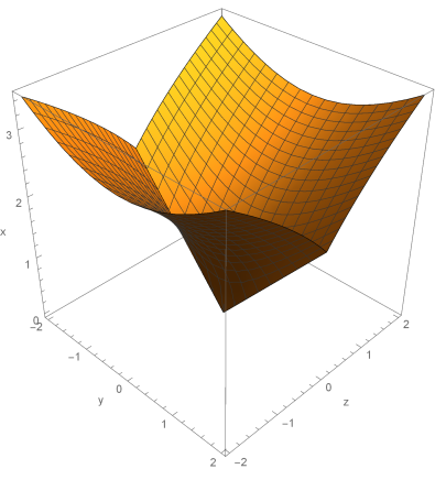
  Figure 1: The Heisenberg beak $\partial\mathcal{A}$

  

  

  Figure 2: View of $\partial\mathcal{A}$ along $y$-axis

  Figure 3: View of $\partial\mathcal{A}$ along $z$-axis

• The lower bound of the sub-Lorentzian distance

  $$\sqrt{x^{2}-y^{2}-4|z|}\leq d(q_{0},q),\qquad q=(x,y,z)\in J^{+}(q_{0}),$$

  was proved. It was also noted that an upper bound

  $$d(q_{0},q)\leq C\sqrt{x^{2}-y^{2}-4|z|}$$

  does not hold for any constant $C\in{\mathbb{R}}$.

• It was proved that there exist non-Hamiltonian maximizers, i.e., maximizers that are not projections of the Hamiltonian vector field $\vec{H}$, $H=\frac{1}{2}(h_{2}^{2}-h_{1}^{2})$, related to the problem.

5 Pontryagin maximum principle

In this section we compute extremal trajectories of the sub-Lorentzian problem $(\ref{prf1})$–$(\ref{prf4})$. The majority of results of this section were obtained by M. Grochowski [12, 13] in another notation, we present these results here for further reference.

Denote points of the cotangent bundle $T^{*}M$ as $\lambda$. Introduce linear on fibers of $T^{*}M$ Hamiltonians $h_{i}(\lambda)=\langle\lambda,X_{i}\rangle$, $i=1,2,3.$ Define the Hamiltonian of the Pontryagin maximum principle (PMP) for the sub-Lorentzian problem $(\ref{prf1})$–$(\ref{prf4})$

$$h_{u}^{\nu}(\lambda)=u_{1}h_{1}(\lambda)+u_{2}h_{2}(\lambda)-\nu\sqrt{u_{1}^{2}-u_{2}^{2}},\qquad\lambda\in T^{*}M,\quad u\in U,\quad\nu\in{\mathbb{R}}.$$

It follows from PMP [19, 4] that if $u(t)$, $t\in[0,t_{1}]$, is an optimal control in problem $(\ref{prf1})$–$(\ref{prf4})$, and $q(t)$, $t\in[0,t_{1}]$, is the corresponding optimal trajectory, then there exists a curve $\lambda_{\cdot}\in\operatorname{Lip}\nolimits([0,t_{1}],T^{*}M)$, $\pi(\lambda_{t})=q(t)$, and a number $\nu\in\{0,-1\}$ for which there hold the conditions for a.e. $t\in[0,t_{1}]$:

1. the Hamiltonian system $\dot{\lambda}_{t}=\vec{h}_{u(t)}^{\nu}(\lambda_{t})$,

2. the maximality condition $h_{u(t)}^{\nu}(\lambda_{t})=\max_{v\in U}h_{v}^{\nu}(\lambda_{t})\equiv 0$,

3. the nontriviality condition $(\nu,\lambda_{t})\neq(0,0)$.

A curve $\lambda_{\cdot}$ that satisfies PMP is called an extremal, and the corresponding control $u(\cdot)$ and trajectory $q(\cdot)$ are called extremal control and trajectory.

5.1 Abnormal case

Theorem 1.

In the abnormal case $\nu=0$ extremals $\lambda_{t}$ and controls $u(t)$ have the following form for some $\tau_{1},\tau_{2}\geq 0$:

• $h_{3}(\lambda_{t})\equiv\operatorname{const}\nolimits>0$:

  $$t\in(0,\tau_{1}) \quad\Rightarrow\quad h_{1}(\lambda_{t})=h_{2}(\lambda_{t})<0,\qquad u_{1}(t)=-u_{2}(t),$$

  $$t\in(\tau_{1},\tau_{1}+\tau_{2}) \quad\Rightarrow\quad h_{1}(\lambda_{t})=-h_{2}(\lambda_{t})<0,\qquad u_{1}(t)=u_{2}(t).$$

• $h_{3}(\lambda_{t})\equiv\operatorname{const}\nolimits<0$:

  $$t\in(0,\tau_{1}) \quad\Rightarrow\quad h_{1}(\lambda_{t})=-h_{2}(\lambda_{t})<0,\qquad u_{1}(t)=u_{2}(t),$$

  $$t\in(\tau_{1},\tau_{1}+\tau_{2}) \quad\Rightarrow\quad h_{1}(\lambda_{t})=h_{2}(\lambda_{t})<0,\qquad u_{1}(t)=-u_{2}(t).$$

• $h_{3}(\lambda_{t})\equiv 0$:

  $$(h_{1},h_{2})(\lambda_{t})\equiv\operatorname{const}\nolimits\neq(0,0),\qquad h_{1}(\lambda_{t})\equiv-|h_{2}(\lambda_{t})|,$$

  $$u(t)\equiv\operatorname{const}\nolimits,\qquad u_{1}(t)\equiv\pm u_{2}(t),\quad\pm=-\operatorname{sgn}\nolimits(h_{1}h_{2}(\lambda_{t})).$$

Proof.

Apply the PMP for the case $\nu=0$. ∎

Corollary 1.

Along abnormal extremals $H(\lambda_{t})\equiv 0$, where $H=\frac{1}{2}(h_{2}^{2}-h_{1}^{2})$.

5.2 Normal case

In the normal case ($\nu=-1$) extremals exist only for $h_{1}\leq-|h_{2}|$. In the case $h_{1}=-|h_{2}|$ normal controls and extremal trajectories coincide with the abnormal ones. And in the domain $\{\lambda\in T^{*}M\mid h_{1}<-|h_{2}|\}$ extremals are reparametrizations of trajectories of the Hamiltonian vector field $\vec{H}$ with the Hamiltonian $H=\frac{1}{2}(h_{2}^{2}-h_{1}^{2})$. In the arclength parametrization, the extremal controls are

$$(u_{1},u_{2})(t)=(-h_{1}(\lambda_{t}),h_{2}(\lambda_{t})),$$ (5.1)

and the extremals satisfy the Hamiltonian ODE $\dot{\lambda}=\vec{H}(\lambda)$ and belong to the level surface $\{H(\lambda)=\frac{1}{2}\}$, in coordinates:

$$\dot{h}_{1}=-{h_{2}h_{3}},\qquad\dot{h}_{2}=-{h_{1}h_{3}},\qquad\dot{h}_{3}=0,$$

$$\dot{q}=\cosh\psi\,X_{1}+\sinh\psi\,X_{2},$$

$$h_{1}=-\cosh\psi,\qquad h_{2}=\sinh\psi,\qquad\psi\in{\mathbb{R}}.$$

We denote $c=h_{3}$ and obtain a parametrization of normal trajectories $q(t)=\pi\circ e^{t\vec{H}}(\lambda_{0})$, $\lambda_{0}\in H^{-1}\left(\frac{1}{2}\right)\cap T^{*}_{q_{0}}M$. If $c=0$, then

$$x=t\cosh\psi,\quad y=t\sinh\psi,\quad z=0.$$ (5.2)

If $c\neq 0$, then

$$x=\frac{\sinh(\psi+ct)-\sinh\psi}{c},\quad y=\frac{\cosh(\psi+ct)-\cosh\psi}{c},\quad z=\frac{\sinh(ct)-ct}{2c^{2}}.$$ (5.3)

Summing up, we obtain the following characterization of normal trajectories in the sub-Lorentzian problem $(\ref{prf1})$–$(\ref{prf4})$.

Theorem 2.

Normal controls and trajectories either coincide with abnormal ones (in the case $h_{1}(\lambda_{t})=-|h_{2}(\lambda_{t})|$, see Th. 1), or can be arclength parametrized to get controls $(\ref{u_norm})$ and future directed timelike trajectories $(\ref{qc=0})$ if $c=0$, or $(\ref{qcn0})$ if $c\neq 0$.

In particular, along each normal extremal $H(\lambda_{t})\equiv\operatorname{const}\nolimits\in\left\{0,\frac{1}{2}\right\}$.

Consequently, normal trajectories are either nonstrictly normal (i.e., simultaneously normal and abnormal) in the case $H=0$, or strictly normal (i.e., normal but not abnormal) in the case $H=\frac{1}{2}$. Strictly normal arclength-parametrized trajectories are described by the exponential mapping

$$\operatorname{Exp}\nolimits\,:\,N\to\widetilde{\mathcal{A}},\qquad(\lambda,t)\mapsto q(t)=\pi\circ e^{t\vec{H}}(\lambda),$$ (5.4)

$$N=C\times{\mathbb{R}}_{+},\qquad{\mathbb{R}}_{+}=(0,+\infty),\qquad C=T^{*}_{\operatorname{Id}\nolimits}M\cap H^{-1}\left(\frac{1}{2}\right)\simeq{\mathbb{R}}^{2}_{\psi,c},$$

$$\widetilde{\mathcal{A}}=\operatorname{int}\nolimits\mathcal{A}=I^{+}(q_{0})$$

given explicitly by formulas $(\ref{qc=0})$, $(\ref{qcn0})$.

In papers [12, 13] were obtained formulas equivalent to $(\ref{qc=0})$, $(\ref{qcn0})$.

Remark 2.

Projections of strictly normal (future directed timelike) trajectories to the plane $(x,y)$ are:

• either rays $y=kx$, $x\geq 0$, $k\in(-1,1)$ (for $c=0$), see Fig. 5,

• or arcs of hyperbolas with asymptotes $x=\pm y>0$ (for $c\neq 0$), see Fig. 5.

Figure 4: Strictly normal $(x(t),y(t))$, $c=0$

Figure 5: Strictly normal $(x(t),y(t))$, $c\neq 0$

Projections of nonstrictly normal (future directed lightlike) trajectories to the plane $(x,y)$ are broken lines with one or two edges parallel to the rays $x=\pm y>0$, see Fig. 6.

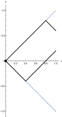
Figure 6: Nonstrictly normal $(x(t),y(t))$

Projections of all extremal trajectories (as well as of all admissible trajectories) to the plane $(x,y)$ are contained in the angle $\{(x,y)\in{\mathbb{R}}^{2}\mid x\geq|y|\}$, which is the projection of the attainable set $J^{+}(q_{0})$ to this plane.

Remark 3.

The Hamiltonian $H=\frac{1}{2}(h_{2}^{2}-h_{1}^{2})$ is preserved on each extremal. On the other hand, since the problem is left-invariant, the extremals respect the symplectic foliation on the dual of the Heisenberg Lie algebra $T^{*}_{\operatorname{Id}\nolimits}M=\{(h_{1},h_{2},h_{3})\}$ consisting of $2$-dimensional symplectic leaves $\{h_{3}=\operatorname{const}\nolimits\neq 0\}$ and $0$-dimensional leaves $\{h_{3}=0,\ (h_{1},h_{2})=\operatorname{const}\nolimits\}$. Thus projections of extremals to $T^{*}_{\operatorname{Id}\nolimits}M=\{(h_{1},h_{2},h_{3})\}$ belong to intersections of the level surfaces $\left\{H=\operatorname{const}\nolimits\in\left\{0,\frac{1}{2}\right\}\right\}$ with the symplectic leaves:

• branches of hyperbolas $h_{1}^{2}-h_{2}^{2}=1$, $h_{1}<0$, $h_{3}\neq 0$,

• points $(h_{1},h_{2})=\operatorname{const}\nolimits$, $H\in\left\{0,\frac{1}{2}\right\}$, $h_{1}\leq-|h_{2}|$, $h_{3}=0$,

• angles $h_{1}=-|h_{2}|$, $h_{3}\neq 0$.

See Figs. 8, 8.

Figure 7: Strictly normal $(h_{1}(t),h_{2}(t),h_{3}(t))$

Figure 8: Nonstrictly normal $(h_{1}(t),h_{2}(t),h_{3}(t))$

Remark 4.

In the sense of work [12], strictly normal extremal trajectories $q(t)=\pi\circ e^{t\vec{H}}(\lambda)$, $\lambda\in C$, are Hamiltonian since they are projections of trajectories of the Hamiltonian vector field $\vec{H}$.

On the other hand, nonstrictly normal extremal trajectories given by items $(1)$, $(2)$ of Th. 1 are non-Hamiltonian, e.g., the broken curves

$$\begin{cases}e^{t(X_{1}+X_{2})},&t\in[0,\tau_{1}],\\ e^{(t-\tau_{1})(X_{1}-X_{2})}\circ e^{\tau_{1}(X_{1}+X_{2})},&t\in[\tau_{1},\tau_{2}],\end{cases}$$ (5.5)

and

$$\begin{cases}e^{t(X_{1}-X_{2})},&t\in[0,\tau_{1}],\\ e^{(t-\tau_{1})(X_{1}+X_{2})}\circ e^{\tau_{1}(X_{1}-X_{2})},&t\in[\tau_{1},\tau_{2}],\end{cases}$$ (5.6)

for $0<\tau_{1}<\tau_{2}$. See item $(5)$ in Sec. 4. Although, each smooth arc of the broken trajectories $(\ref{broken+-})$, $(\ref{broken-+})$ is a reparametrization of projection of a trajectory of the Hamiltonian vector field $\vec{H}$ contained in a face of the angle $\{(h_{1},h_{2},h_{3})\in T_{\operatorname{Id}\nolimits}^{*}M\mid h_{1}=-|h_{2}|\}$, see Fig. 8.

6 Inversion of the exponential mapping

Theorem 3.

The exponential mapping $\operatorname{Exp}\nolimits\,:\,N\to\widetilde{\mathcal{A}}$ is a real-analytic diffeomorphism. The inverse mapping $\operatorname{Exp}\nolimits^{-1}\,:\,\widetilde{\mathcal{A}}\to N$, $(x,y,z)\mapsto(\psi,c,t)$, is given by the following formulas:

$$z=0\quad\Rightarrow\quad\psi=\operatorname{artanh}\nolimits\frac{y}{x},\quad c=0,\quad t=\sqrt{x^{2}-y^{2}},$$ (6.1)

$$z\neq 0\quad\Rightarrow\quad\psi=\operatorname{artanh}\nolimits\frac{y}{x}-p,\quad c=(\operatorname{sgn}\nolimits z)\sqrt{\frac{\sinh 2p-2p}{2z}},\quad t=\frac{2p}{c},$$ (6.2)

where $p=\beta\left(\frac{z}{x^{2}-y^{2}}\right)$, and $\beta\,:\,\left(-\frac{1}{4},\frac{1}{4}\right)\to{\mathbb{R}}$ is the inverse function to the diffeomorphism

$$\alpha\,:\,{\mathbb{R}}\to\left(-\frac{1}{4},\frac{1}{4}\right),\qquad\alpha(p)=\frac{\sinh 2p-2p}{8\sinh^{2}p}.$$

See plots of the functions $\alpha(p)$ and $\beta(z)$ in Figs. 10 and 10 respectively.

Figure 9: Plot of $\alpha(p)$

Figure 10: Plot of $\beta(z)$

Proof.

The exponential mapping is real-analytic since the strictly normal extremals are trajectories of the real-analytic Hamiltonian vector field $\vec{H}$. We show that $\operatorname{Exp}\nolimits$ is bijective.

Formulas $(\ref{invz0})$ follow immediately from $(\ref{qc=0})$.

Let $c\neq 0$. Then formulas $(\ref{qcn0})$ yield

$$x=\frac{2}{c}\sinh p\cosh\tau,\quad y=\frac{2}{c}\sinh p\sinh\tau,\quad z=\frac{1}{2c^{2}}(\sinh 2p-2p),$$ (6.3)

$$p=\frac{ct}{2},\qquad\tau=\psi+\frac{ct}{2}.$$ (6.4)

Thus

$$x^{2}-y^{2}=\frac{4}{c^{2}}\sinh^{2}p,$$ (6.5)

$$\frac{z}{x^{2}-y^{2}}=\frac{\sinh 2p-2p}{8\sinh^{2}p}=\alpha(p).$$

The function $\alpha(p)$ is a diffeomorphism from ${\mathbb{R}}$ to $\left(-\frac{1}{4},\frac{1}{4}\right)$, thus it has an inverse function, a diffeomorphism $\beta\,:\,\left(-\frac{1}{4},\frac{1}{4}\right)\to{\mathbb{R}}$. So $p=\beta(\frac{z}{x^{2}-y^{2}})$. Now formulas $(\ref{invzn0})$ follow from $(\ref{xyznew})$, $(\ref{ptau})$.

So $\operatorname{Exp}\nolimits$ is a smooth bijection with a smooth inverse, i.e., a diffeomorphism. ∎

7 Optimality of extremal trajectories

We study optimality of extremal trajectories. The main tool is a sufficient optimality condition (Th. 4) based on a field of extremals (see [4], Sec. 17.1).

We prove optimality of all extremal trajectories (Theorems 7, 8) without apriori theorem on existence of optimal trajectories. Such a theorem was recently proved [21], and it can shorten the proof of optimality in our work.

7.1 Sufficient optimality condition

Let $M$ be a smooth manifold, then the cotangent bundle $T^{*}M$ bears the Liouville 1-form $s=pdq\in\Lambda^{1}(T^{*}M)$ and the symplectic 2-form $\sigma=ds=dp\wedge dq\in\Lambda^{2}(T^{*}M)$. A submanifold $\mathcal{L}\subset T^{*}M$ is called a Lagrangian manifold if $\dim\mathcal{L}=\dim M$ and $\left.\sigma\right|_{\mathcal{L}}=0$.

Consider an optimal control problem

$$\dot{q}=f(q,u),\qquad q\in M,\quad u\in U,$$

$$q(t_{0})=q_{0},\qquad q(t_{1})=q_{1},$$

$$J[q(\cdot)]=\int_{t_{0}}^{t_{1}}\varphi(q,u)\,dt\to\min,$$

$$t_{0}\text{ is fixed},\qquad t_{1}\text{ is free}.$$

Let $g_{u}(\lambda)=\langle\lambda,f(q,u)\rangle-\varphi(q,u)$, $\lambda\in T^{*}M$, $q=\pi(\lambda)$, $u\in U$, be the normal Hamiltonian of PMP. Suppose that the maximized normal Hamiltonian $G(\lambda)=\max_{u\in U}g_{u}(\lambda)$ is smooth in an open domain $O\subset T^{*}M$, and let the Hamiltonian vector field $\vec{G}\in\operatorname{Vec}\nolimits(O)$ be complete.

Theorem 4.

Let $\mathcal{L}\subset G^{-1}(0)\cap O$ be a Lagrangian submanifold such that the form $\left.s\right|_{\mathcal{L}}$ is exact. Let the projection $\pi\,:\,\mathcal{L}\to\pi(\mathcal{L})$ be a diffeomorphism on a domain in $M$. Consider an extremal $\widetilde{\lambda}_{t}=e^{t\vec{G}}(\lambda_{0})$, $t\in[t_{0},t_{1}]$, contained in $\mathcal{L}$, and the corresponding extremal trajectory $\widetilde{q}(t)=\pi(\widetilde{\lambda}_{t})$. Consider also any trajectory $q(t)\in\pi(\mathcal{L})$, $t\in[t_{0},\tau]$, such that $q(t_{0})=\widetilde{q}(t_{0})$, $q(\tau)=\widetilde{q}(t_{1})$. Then $J[\widetilde{q}(\cdot)]<J[q(\cdot)]$.

Proof.

Completely similarly to the proof of Th. 17.2 [4]. ∎

7.2 Optimality in the reduced sub-Lorentzian problem
on the Heisenberg group

We apply Th. 4 to the reduced sub-Lorentzian problem $(\ref{pr31})$–$(\ref{pr34})$. For this problem the maximized Hamiltonian $G=1-\sqrt{h_{1}^{2}-h^{2}_{2}}$ is smooth on the domain $O=\{\lambda\in T^{*}M\mid h_{1}<-|h_{2}|\}$, and the Hamiltonian vector field $\vec{G}\in\operatorname{Vec}\nolimits(O)$ is complete. In the domain $O$ the Hamiltonian vector fields $\vec{G}$ and $\vec{H}$ have the same trajectories up to a monotone time reparametrization; moreover, on the level surface $\left\{H=\frac{1}{2}\right\}=\{G=0\}$ they just coincide between themselves.

Define the set

$$\mathcal{L}=\left\{e^{t\vec{G}}(\lambda_{0})\mid\lambda_{0}\in C,\ t>0\right\}.$$ (7.1)

Lemma 1.

$\mathcal{L}\subset T^{*}M$ is a Lagrangian manifold such that $\left.s\right|_{\mathcal{L}}$ is exact.

Proof.

Consider a smooth mapping

$$\Phi\,:\,(T^{*}_{\operatorname{Id}\nolimits}M\cap G^{-1}(0))\times{\mathbb{R}}_{+}\to T^{*}M,\qquad(\lambda_{0},t)\mapsto e^{t\vec{G}}(\lambda_{0}).$$

Since

$$\operatorname{rank}\nolimits\left(\frac{\partial\,\Phi}{\partial\,(t,\lambda_{0})}\right) =\operatorname{rank}\nolimits\left(\vec{G}(\lambda),e^{t\vec{G}}_{*}\left(h_{2}\frac{\partial\,}{\partial\,h_{1}}+h_{1}\frac{\partial\,}{\partial\,h_{2}}\right),e^{t\vec{G}}_{*}\frac{\partial\,}{\partial\,h_{3}}\right)$$

$$=\operatorname{rank}\nolimits\left(\vec{G}(\lambda_{0}),h_{2}\frac{\partial\,}{\partial\,h_{1}}+h_{1}\frac{\partial\,}{\partial\,h_{2}},\frac{\partial\,}{\partial\,h_{3}}\right)$$

$$=\operatorname{rank}\nolimits\left(-h_{1}X_{1}+h_{2}X_{2},h_{2}\frac{\partial\,}{\partial\,h_{1}}+h_{1}\frac{\partial\,}{\partial\,h_{2}},\frac{\partial\,}{\partial\,h_{3}}\right)$$

$$=3,$$

then $\mathcal{L}$ is a smooth 3-dimensional manifold.

Further, $\pi(\mathcal{L})=\operatorname{Exp}\nolimits(N)=\widetilde{\mathcal{A}}$ by Th. 3. Moreover, since $\operatorname{Exp}\nolimits=\pi\circ\Phi$ and $\operatorname{Exp}\nolimits\,:\,N\to\widetilde{\mathcal{A}}$ is a diffeomorphism by Th. 3, then $\pi\,:\,\mathcal{L}\to\widetilde{\mathcal{A}}$ is a diffeomorphism as well.

Let us show that $\left.\sigma\right|_{\mathcal{L}}=0$. Take any $\lambda=e^{t\vec{G}}(\lambda_{0})\in\mathcal{L}$, $(\lambda_{0},t)\in N$, then $T_{\lambda}\mathcal{L}={\mathbb{R}}\vec{G}(\lambda)\oplus e^{t\vec{G}}_{*}(T_{\lambda_{0}}C)$. Take any two vectors $T_{\lambda}\mathcal{L}\ni v_{i}=r_{i}\vec{G}(\lambda)+e^{t\vec{G}}_{*}w_{i}$, $w_{i}\in T_{\lambda_{0}}C$, $i=1,2$. Then

$$\sigma(v_{1},v_{2})=r_{1}\sigma(\vec{G}(\lambda_{0}),w_{2})+r_{2}\sigma(w_{1},\vec{G}(\lambda_{0}))=0$$

since $\sigma(w_{i},\vec{G}(\lambda_{0}))=\langle dG,w_{i}\rangle=0$ by virtue of $w_{i}\in T_{\lambda_{0}}C=\{dG=0\}$.

So the 1-form $\left.s\right|_{\mathcal{L}}$ is closed. But $\widetilde{\mathcal{A}}$ is simply connected, thus $\mathcal{L}$ is simply connected as well. Consequently, $\left.s\right|_{\mathcal{L}}$ is exact by the Poincaré lemma. ∎

Theorem 5.

For any point $q_{1}\in\operatorname{int}\nolimits\mathcal{A}=I^{+}(q_{0})$ the strictly normal trajectory $q(t)=\operatorname{Exp}\nolimits(\lambda,t)$, $t\in[0,t_{1}]$, is the unique optimal trajectory of the reduced sub-Lorentzian problem $(\ref{pr31})$–$(\ref{pr34})$ connecting $q_{0}$ with $q_{1}$, where $(\lambda,t_{1})=\operatorname{Exp}\nolimits^{-1}(q_{1})\in N$.

Proof.

Take any $\lambda_{0}\in C$, $t_{1}>t_{0}>0$. Then the Lagrangian manifold $\mathcal{L}$ $(\ref{L})$ and the extremal $\widetilde{\lambda}_{t}=e^{t\vec{G}}(\lambda_{0})$, $t\in[t_{0},t_{1}]$, satisfy hypotheses of Th. 4. Thus the trajectory $\widetilde{q}(t)=\pi(\widetilde{\lambda}_{t})$, $t\in[t_{0},t_{1}]$, is a strict maximizer for the reduced sub-Lorentzian problem $(\ref{pr31})$–$(\ref{pr34})$.

Take any $\lambda_{1}\in C$, $t_{2}>0$, and consider the extremal trajectory $\bar{q}(t)=\operatorname{Exp}\nolimits(\lambda_{1},t)$, $t\in[0,t_{2}]$. Take any $\widehat{q}\in\widetilde{\mathcal{A}}$. The set $\mathcal{A}$ is an attainable set of a left-invariant control system on a Lie group, thus it is a semigroup. Consequently, $\widehat{q}\cdot\bar{q}(t)$ is an extremal trajectory contained in $\widetilde{\mathcal{A}}$. By the previous paragraph, this trajectory is a strict maximizer for the reduced sub-Lorentzian problem $(\ref{pr31})$–$(\ref{pr34})$. By left invariance of this problem, the same holds for the trajectory $\bar{q}(t)$, $t\in[0,t_{2}]$. ∎

Denote the cost function for the equivalent reduced sub-Lorentzian problems $(\ref{pr21})$–$(\ref{pr24})$ and $(\ref{pr31})$–$(\ref{pr34})$:

$$\widetilde{d}(q_{1}) =\sup\{l(q(\cdot))\mid\text{ traj. $q(\cdot)$ of $(\ref{pr21})$--$(\ref{pr24})$, $q(0)=q_{0}$, $q(t_{1})=q_{1}$}\}$$

$$=\sup\{t_{1}>0\mid\exists\text{ traj. $q(\cdot)$ of $(\ref{pr31})$--$(\ref{pr34})$ s.t. $q(0)=q_{0}$, $q(t_{1})=q_{1}$}\},$$

where $q_{1}\in\operatorname{int}\nolimits\mathcal{A}=I^{+}(q_{0})$. This function has the following description and regularity property.

Theorem 6.

Let $q=(x,y,z)\in I^{+}(q_{0})$. Then

$$\widetilde{d}(q)=\sqrt{x^{2}-y^{2}}\cdot\frac{p}{\sinh p},\qquad p=\beta\left(\frac{z}{x^{2}-y^{2}}\right).$$ (7.2)

The function $\widetilde{d}\,:\,I^{+}(q_{0})\to{\mathbb{R}}_{+}$ is real-analytic.

Proof.

Let $q\in I^{+}(q_{0})$, then the sub-Lorentzian length maximizer from $q_{0}$ to $q$ for the reduced sub-Lorentzian problem $(\ref{pr31})$–$(\ref{pr34})$ is described in Th. 5, and the expression for $\widetilde{d}(q)$ in $(\ref{tdq})$ follows from the expression for $t$ in $(\ref{invzn0})$.

The both functions $\sqrt{x^{2}-y^{2}}$ and $\frac{p}{\sinh p}$ are real-analytic on $I^{+}(q_{0})$, thus $\widetilde{d}$ is real-analytic as well. ∎

7.3 Optimality in the full sub-Lorentzian problem
on the Heisenberg group

In this subsection we consider the full sub-Lorentzian problem $(\ref{prf1})$–$(\ref{prf4})$.

Theorem 7.

Let $q_{1}\in I^{+}(q_{0})$. Then the sub-Lorentzian length maximizers for the full problem $(\ref{prf1})$–$(\ref{prf4})$ are reparametrizations of the corresponding sub-Lorentzian length maximizer for the reduced problem $(\ref{pr31})$–$(\ref{pr34})$ described in Th. 5.

In particular, $\left.d\right|_{I^{+}(q_{0})}=\widetilde{d}$.

Proof.

Let $q(t)$, $t\in[0,t_{1}]$, be a trajectory of the full problem $(\ref{prf1})$–$(\ref{prf4})$ such that $q(0)=q_{0}$, $q(t_{1})=q_{1}$, and let $q(\cdot)$ be not a trajectory of the reduced problem $(\ref{pr21})$–$(\ref{pr24})$ (that is, there exist $0\leq\tau_{1}<\tau_{2}\leq t_{1}$ such that $\left.\left(u_{1}-|u_{2}|\right)\right|_{[\tau_{1},\tau_{2}]}\equiv 0$). Let $\widetilde{q}(t)$, $t\in[0,\widetilde{t}_{1}]$, be the optimal trajectory in the reduced problem $(\ref{pr31})$–$(\ref{pr34})$ connecting $q_{0}$ with $q_{1}$. We show that $l(q(\cdot))<l(\widetilde{q}(\cdot))$. By contradiction, suppose that $l(q(\cdot))\geq l(\widetilde{q}(\cdot))$.

Let $l(q(\cdot))=l(\widetilde{q}(\cdot))$. The trajectory $q(\cdot)$ does not satisfy the PMP for the full problem $(\ref{prf1})$–$(\ref{prf4})$ (see Sec. 5), thus it is not optimal in this problem. Thus there exists a trajectory $\bar{q}(\cdot)$ of this problem with the same endpoints and $l(\bar{q}(\cdot))>l(\widetilde{q}(\cdot))$. The curve $\bar{q}(\cdot)$ cannot be a trajectory of the reduced system since its length is greater than the maximum $l(\widetilde{q}(\cdot))$ in this problem. So we can denote $\bar{q}(\cdot))$ as $q(\cdot)$ and assume that $l(q(\cdot))>l(\widetilde{q}(\cdot))$.

After time reparametrization we obtain that the control $u(t)=(u_{1}(t),u_{2}(t))$ corresponding to the trajectory $q(t)$, $t\in[0,t_{1}]$, satisfies $u_{1}(t)\equiv 1$, thus $|u_{2}(t)|\leq 1$.

For any $\delta\in(0,1)$ define a function

$$u_{2}^{\delta}(t)=\begin{cases}u_{2}(t)&\text{for }|u_{2}(t)|\leq 1-\delta,\\ 1-\delta&\text{for }u_{2}(t)>1-\delta,\\ \delta-1&\text{for }u_{2}(t)<\delta-1,\end{cases}$$

so that

$$|u_{2}^{\delta}(t)|\leq 1-\delta,\quad|u_{2}^{\delta}(t)-u_{2}(t)|\leq\delta,\qquad t\in[0,t_{1}].$$ (7.3)

Define an admissible control $u^{\delta}(t)=(1,u_{2}^{\delta}(t))$, $t\in[0,t_{1}]$, and consider the corresponding trajectory $q^{\delta}(t)$, $t\in[0,t_{1}]$, of the reduced problem $(\ref{pr21})$–$(\ref{pr24})$ with $q^{\delta}(0)=q_{0}$. Denote its endpoint $q^{\delta}(t_{1})=q_{1}^{\delta}$. By virtue of the second inequality in $(\ref{u2de})$,

$$l(q^{\delta}(\cdot))=\int_{0}^{t_{1}}\sqrt{1-\left(u_{2}^{\delta}(t)\right)^{2}}dt\to\int_{0}^{t_{1}}\sqrt{1-u_{2}^{2}(t)}dt=l(q(\cdot)),$$

$$\max_{t\in[0,t_{1}]}\|q^{\delta}(t)-q(t)\|\to 0$$

as $\delta\to+0$. So for sufficiently small $\delta>0$ we have

$$l(q^{\delta}(\cdot))>l(\widetilde{q}(\cdot))\qquad\text{and}\qquad\|q_{1}^{\delta}-q_{1}\|\text{ is small},$$

where $\|\cdot\|$ is any norm in $M\cong{\mathbb{R}}^{3}$. In particular, $q_{1}^{\delta}\in I^{+}(q_{0})$ for small $\delta>0$.

Now let $\widehat{q}^{\delta}(t)$, $t\in\left[0,\widehat{t}_{1}^{\delta}\right]$, be the optimal trajectory in the reduced problem $(\ref{pr31})$–$(\ref{pr34})$ with the boundary conditions $\widehat{q}^{\delta}(0)=q_{0}$, $\widehat{q}^{\delta}\left(\widehat{t}_{1}^{\delta}\right)=q_{1}^{\delta}$. Then for small $\delta>0$

$$l\left(\widehat{q}^{\delta}(\cdot)\right)\geq l(q^{\delta}(\cdot))>l(\widetilde{q}(\cdot)),$$

$$\left\|q_{1}^{\delta}-q_{1}\right\|=\left\|\widehat{q}^{\delta}\left(\widehat{t}_{1}^{\delta}\right)-\widetilde{q}(t_{1})\right\|\text{ is small}.$$

By virtue of Th. 6, the sub-Lorentzian distance $\widetilde{d}\,:\,I^{+}(q_{0})\to{\mathbb{R}}_{+}$ in the reduced problem $(\ref{pr31})$–$(\ref{pr34})$ is continuous, thus for small $\delta>0$

$$|l\left(\widehat{q}^{\delta}(\cdot)\right)-l(\widetilde{q}(\cdot))|=|\widetilde{d}(q_{1}^{\delta})-\widetilde{d}(q_{1})|\text{ is small}.$$

Summing up, for small $\delta>0$ the difference

$$l(q(\cdot))-l(\widetilde{q}(\cdot))<\left(l(q(\cdot))-l\left(q^{\delta}(\cdot)\right)\right)+\left(l\left(\widehat{q}^{\delta}(\cdot)\right)-l\left(\widetilde{q}(\cdot)\right)\right)$$

becomes arbitrarily small, a contradiction. Thus $\widetilde{q}(\cdot)$ is optimal and $q(\cdot)$ is not optimal in the full sub-Lorentzian problem $(\ref{prf1})$–$(\ref{prf4})$. ∎

Theorem 8.

Let $q_{1}=(x_{1},y_{1},z_{1})\in\partial A=J^{+}(q_{0})\setminus I^{+}(q_{0})$, $q_{1}\neq q_{0}$. Then an optimal trajectory in the full sub-Lorentzian problem $(\ref{prf1})$–$(\ref{prf4})$ is a future directed lightlike piecewise smooth trajectory with one or two subarcs generated by the vector fields $X_{1}\pm X_{2}$. In detail, up to a reparametrization:

• If $z_{1}=0$, then

  $$u(t)\equiv\operatorname{const}\nolimits=(1,\pm 1),\qquad q(t)=e^{t(X_{1}\pm X_{2})}=(t,\pm t,0),\qquad t\in[0,t_{1}],\quad t_{1}=x_{1}.$$

• If $z_{1}>0$, then

  $$t\in[0,\tau_{1}]\quad\Rightarrow\quad u(t)\equiv(1,-1),\qquad q(t)=e^{t(X_{1}-X_{2})}=(t,-t,0),$$

  $$t\in[\tau_{1},\tau_{1}+\tau_{2}]\quad\Rightarrow\quad u(t)\equiv(1,1),$$

  $$\qquad\qquad\qquad q(t)=e^{(t-\tau_{1})(X_{1}+X_{2})}e^{\tau_{1}(X_{1}-X_{2})}=(t,t-2\tau_{1},\tau_{1}(t-\tau_{1})),$$

  $$\tau_{1}=\frac{x_{1}-y_{1}}{2},\qquad\tau_{2}=\frac{x_{1}+y_{1}}{2}.$$

• If $z_{1}<0$, then

  $$t\in[0,\tau_{1}]\quad\Rightarrow\quad u(t)\equiv(1,1),\qquad q(t)=e^{t(X_{1}+X_{2})}=(t,t,0),$$

  $$t\in[\tau_{1},\tau_{1}+\tau_{2}]\quad\Rightarrow\quad u(t)\equiv(1,-1),$$

  $$\qquad\qquad\qquad q(t)=e^{(t-\tau_{1})(X_{1}-X_{2})}e^{\tau_{1}(X_{1}+X_{2})}=(t,2\tau_{1}-t,-\tau_{1}(t-\tau_{1})),$$

  $$\tau_{1}=\frac{x_{1}+y_{1}}{2},\qquad\tau_{2}=\frac{x_{1}-y_{1}}{2}.$$

The broken lightlike trajectories with two arcs described in items (1), (2) of Th. 8 are shown in Fig. 22.

Proof.

Let $q(t)$, $t\in[0,t_{1}]$, be a future directed nonspacelike trajectory connecting $q_{0}$ and $q_{1}$. If $q(\cdot)$ is not lightlike, then there exists a future directed timelike arc $q(t)$, $t\in[s_{1},s_{2}]$, $0\leq s_{1}<s_{2}\leq t_{1}$, thus $q(t_{1})\in\operatorname{int}\nolimits\mathcal{A}$, a contradiction. Thus $q(\cdot)$ is lightlike, and the statement follows by direct computation of trajectories of the lightlike vector fields $X_{1}\pm X_{2}$. ∎

Corollary 2.

For any $q_{1}\in J^{+}(q_{0})$, $q_{1}\neq q_{0}$, there is a unique, up to reparametrization, sub-Lorentzian length minimizer in the full problem $(\ref{prf1})$–$(\ref{prf4})$ that connects $q_{0}$ and $q_{1}$:

• if $q_{1}\in\operatorname{int}\nolimits\mathcal{A}=I^{+}(q_{0})$, then $q(\cdot)$ is a future directed timelike strictly normal trajectory described in Theorems 5, 7.

• if $q_{1}\in\partial\mathcal{A}=J^{+}(q)\setminus I^{+}(q_{0})$, then $q(\cdot)$ is a future directed lightlike nonstrictly normal trajectory described in Th. 8.

Corollary 3.

Any sub-Lorentzian length maximizer of problem $(\ref{prf1})$–$(\ref{prf4})$ of positive length is timelike and strictly normal.

Remark 5.

The broken trajectories described in items $(2)$, $(3)$ of Th. 8 are optimal in the sub-Lorentzian problem, while in sub-Riemannian problems trajectories with angle points cannot be optimal, see [20]. Moreover, these broken trajectories are normal and nonsmooth, which is also impossible in sub-Riemannian geometry.

8 Sub-Lorentzian distance

Denote $d(q):=d(q_{0},q)$, $q\in J^{+}(q_{0})$.

Theorem 9.

Let $q=(x,y,z)\in J^{+}(q_{0})$. Then

$$d(q)=\sqrt{x^{2}-y^{2}}\cdot\frac{p}{\sinh p},\qquad p=\beta\left(\frac{z}{x^{2}-y^{2}}\right).$$ (8.1)

In particular:

• $z=0\iff d(q)=\sqrt{x^{2}-y^{2}}$,
  

• $q\in J^{+}(q_{0})\setminus I^{+}(q_{0})\iff d(q)=0$.

Remark 6.

In the right-hand side of the first equality in $(\ref{dq})$, we assume by continuity that $\frac{p}{\sinh p}=1$ for $p=0$ and $\frac{p}{\sinh p}=0$ for $p=\infty$. See the plot of the function $\frac{p}{\sinh p}$ in Fig. 11.

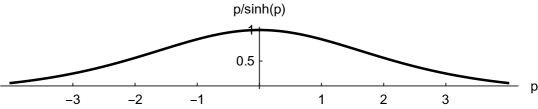
Figure 11: Plot of $\frac{p}{\sinh p}$

Proof.

Let $q\in I^{+}(q_{0})$, then the sub-Lorentzian length maximizers from $q_{0}$ to $q$ are described in Theorem 7 and the expression for $\left.d\right|_{\widetilde{\mathcal{A}}}=\widetilde{d}$ was obtained in Th. 6. In particular, if $z=0$, then $p=0$ and $d(q)=\sqrt{x^{2}-y^{2}}$, and vice versa.

Let $q\in J^{+}(q_{0})\setminus I^{+}(q_{0})$, then the sub-Lorentzian length maximizers from $q_{0}$ to $q$ are described in Th. 8. Thus $d(q)=0$, which agrees with $(\ref{dq})$ since in this case $\frac{|z|}{x^{2}-y^{2}}=\frac{1}{4}$, so $p=\infty$. ∎

We plot restrictions of the sub-Lorentzian distance to several planar domains:

• $\left.d\right|_{z=0}=\sqrt{x^{2}-y^{2}}$ to the domain $J^{+}(q_{0})\cap\{z=0\}=\{x\geq|y|,\ z=0\}$, see Fig. 13,

• $\left.d\right|_{y=0}$ to the domain $J^{+}(q_{0})\cap\{y=0\}=\{-x^{2}/4\leq z\leq x^{2}/4,\ y=0\}$, see Fig. 13,

• $\left.d\right|_{x=1}$ to the domain $J^{+}(q_{0})\cap\{x=1\}=\{y^{2}+4|z|\leq 1,\ x=1\}$, see Fig. 14.

Figure 12: Plot of $\left.d\right|_{z=0}$

Figure 13: Plot of $\left.d\right|_{y=0}$

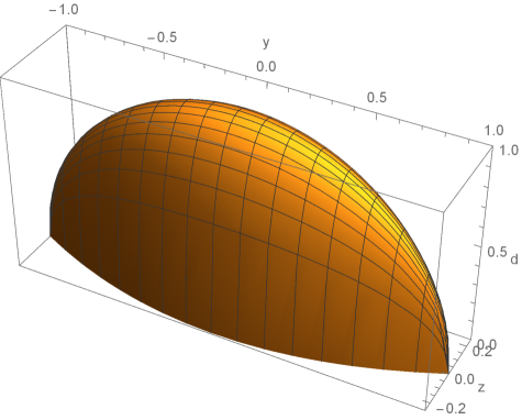
Figure 14: Plot of $\left.d\right|_{x=1}$

The sub-Lorentzian distance has the following regularity properties.

Theorem 10.

• The function $d(\cdot)$ is continuous on $J^{+}(q_{0})$ and real-analytic on $I^{+}(q_{0})$.

• The function $d(\cdot)$ is not Lipschitz near points $q=(x,y,z)$ with $x=|y|>0$, $z=0$.

Proof.

(1) follows from representation $(\ref{dq})$.

(2) follows from item (1) of Th. 9 since the function $\left.d\right|_{z=0}=\sqrt{x^{2}-y^{2}}$ is not Lipschitz near points with $x=|y|>0$. ∎

Remark 7.

Item $(1)$ of Th. 10 improves item $(2)$ of Sec. 4.

Remark 8.

Item $(2)$ of Th. 10 is visualized in Fig. 13 since the cone given by the plot of $\left.d\right|_{z=0}=\sqrt{x^{2}-y^{2}}$ has vertical tangent planes at points $x=|y|>0$.

Moreover, item $(2)$ of Th. 10 can be essentially detailed by a precise description of the asymptotics of the sub-Lorentzian distance $d(q)$ as $q\to\partial\mathcal{A}$, this will be done in a forthcoming paper [22].

Remark 9.

The sub-Lorentzian distance $d\,:\,J^{+}(q_{0})\to[0,+\infty)$ is not uniformly continuous since the same holds for its restriction $\left.d\right|_{z=0}=\sqrt{x^{2}-y^{2}}$ on the angle $\{x\geq|y|\}$.

As was shown in [13], the sub-Lorentzian distance $d(q)$ admits a lower bound by the function $\sqrt{x^{2}-y^{2}-4|z|}$ and does not admit an upper bound by this function multiplied by any constant (see item (4) in Sec. 4). Here we precise this statement and prove another upper bound.

Theorem 11.

• The ratio $\dfrac{\sqrt{x^{2}-y^{2}-4|z|}}{d(q)}$ takes any values in the segment $[0,1]$ for $q=(x,y,z)\in J^{+}(q_{0})$.

• For any $q=(x,y,z)\in J^{+}(q_{0})$ there holds the bound $d(q)\leq\sqrt{x^{2}-y^{2}}$, moreover, the ratio $\dfrac{d(q)}{\sqrt{x^{2}-y^{2}}}$ takes any values in the segment $[0,1]$.

The two-sided bound

$${\sqrt{x^{2}-y^{2}-4|z|}}\leq{d(q)}\leq\sqrt{x^{2}-y^{2}},\qquad q\in J^{+}(q_{0}),$$ (8.2)

is visualized in Fig. 15, which shows plots of the surfaces (from below to top):

$$\sqrt{x^{2}-y^{2}}=1,\qquad{d(q)}=1,\qquad{\sqrt{x^{2}-y^{2}-4|z|}}=1,\qquad q\in J^{+}(q_{0}).$$

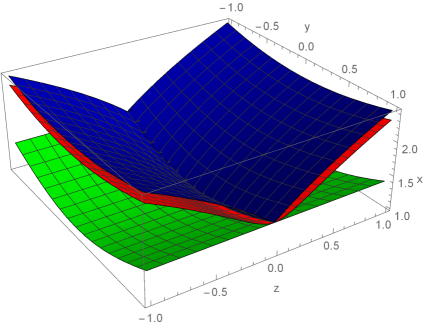
Figure 15: Bound $(\ref{bound})$

Proof.

$(1)$ It follows from $(\ref{dq})$ that

$$\frac{x^{2}-y^{2}-4|z|}{d^{2}(q)}=\frac{\sinh^{2}p-\sinh p\cosh p+p}{p^{2}},$$

and the function in the right-hand side takes all values in the segment $[0,1]$ for $q\in J^{+}(q_{0})$.

$(2)$ It follows from $(\ref{dq})$ that $\frac{d(q)}{\sqrt{x^{2}-y^{2}}}=\frac{p}{\sinh p}$. When $q\in J^{+}(q_{0})$, the ratio $\frac{p}{\sinh p}$ takes all values in the segment $[0,1]$, see Remark 6 after Th. 9. ∎

9 Symmetries

Theorem 12.

• The hyperbolic rotations $X_{0}=y\frac{\partial\,}{\partial\,x}+x\frac{\partial\,}{\partial\,y}$ and reflections $\varepsilon^{1}\ :\ (x,y,z)\mapsto(x,-y,z)$, $\varepsilon^{2}\ :\ (x,y,z)\mapsto(x,y,-z)$ preserve $d(\cdot)$.

• The dilations $Y=x\frac{\partial\,}{\partial\,x}+y\frac{\partial\,}{\partial\,y}+2z\frac{\partial\,}{\partial\,z}$ stretch $d(\cdot)$:

  $$d(e^{sY}(q))=e^{s}d(q),\qquad s\in{\mathbb{R}},\quad q\in J^{+}(q_{0}).$$

Proof.

(1) The flow of the hyperbolic rotations

$$e^{sX_{0}}\ :\ (x,y,z)\mapsto(x\cosh s+y\sinh s,x\sinh s+y\cosh s,z),\qquad s\in{\mathbb{R}},\quad(x,y,z)\in M,$$

preserves the exponential mapping:

$$e^{sX_{0}}\circ\operatorname{Exp}\nolimits(\psi,c,t)=\operatorname{Exp}\nolimits(\psi+s,c,t),\qquad(\psi,c,t)\in N,\quad s\in{\mathbb{R}},$$

thus $d(e^{sX_{0}}(q))=d(q)$ for $q\in I^{+}(q_{0})$. Moreover, the flow $e^{sX_{0}}$ preserves the boundary $\partial\mathcal{A}=J^{+}(q_{0})\setminus I^{+}(q_{0})$, thus $d(e^{sX_{0}}(q))=d(q)=0$ for $q\in J^{+}(q_{0})\setminus I^{+}(q_{0})$.

Further, it is obvious from $(\ref{dq})$ that the reflections $\varepsilon^{1}$, $\varepsilon^{2}$ preserve $d(\cdot)$.

(2) The flow of the dilations

$$e^{sY}\ :\ (x,y,z)\mapsto(xe^{s},ye^{s},ze^{2s}),\qquad s\in{\mathbb{R}},\quad(x,y,z)\in M,$$

acts on the exponential mapping as follows:

$$e^{sY}\circ\operatorname{Exp}\nolimits(\psi,c,t)=\operatorname{Exp}\nolimits(\psi,ce^{-2s},te^{s}),\qquad(\psi,c,t)\in N,\quad s\in{\mathbb{R}},$$

thus $d(e^{sY}(q))=e^{s}d(q)$ for $q\in I^{+}(q_{0})$. The equality $d(e^{sY}(q))=e^{s}d(q)=0$ for $q\in J^{+}(q_{0})\setminus I^{+}(q_{0})$ follows since the flow $e^{sY}$ preserves the boundary $\partial\mathcal{A}=J^{+}(q_{0})\setminus I^{+}(q_{0})$. ∎

10 Sub-Lorentzian spheres

10.1 Spheres of positive radius

Sub-Lorentzian spheres

$$S(R)=\{q\in M\mid d(q)=R\},\qquad R>0,$$

are transformed one into another by dilations:

$$S(e^{s}R)=e^{sY}(S(R)),\qquad s\in{\mathbb{R}},$$

thus we describe the unit sphere

$$S=S(1)=\{\operatorname{Exp}\nolimits(\lambda,1)\mid\lambda\in C\}.$$ (10.1)

Theorem 13.

• The unit sub-Lorentzian sphere $S$ is a regular real-analytic manifold diffeomorphic to ${\mathbb{R}}^{2}$.

• Let $q=\operatorname{Exp}\nolimits(\psi,c,1)\in S$, $(\psi,c)\in C$, then the tangent space

  $$T_{q}S=\left\{v=\sum_{i=1}^{3}v_{i}X_{i}(q)\mid-v_{1}\cosh(\psi+c)+v_{2}\sinh(\psi+c)+v_{3}c=0\right\}.$$ (10.2)

• $S$ is the graph of the function $x=\sqrt{y^{2}+f(z)}$, where $f(z)=e\circ k(z)$, $e(w)=\frac{\sinh^{2}w}{w^{2}}$, $k(z)=b(z)/2$, $b=a^{-1}$, $a(c)=\frac{\sinh c-c}{2c^{2}}$.

• The function $f(z)$ is real-analytic, even, strictly convex, unboundedly and strictly increasing for $z\geq 0$. This function has a Taylor decomposition $f(z)=1+12z^{2}+O(z^{4})$ as $z\to 0$ and an asymptote $4|z|$ as $z\to\infty$:

  $$\lim_{z\to\infty}(f(z)-4|z|)=0.$$ (10.3)

• The function $f(z)$ satisfies the bounds

  $$4|z|<f(z)<4|z|+1,\qquad z\neq 0.$$ (10.4)

• A section of the sphere $S$ by a plane $\{z=\operatorname{const}\nolimits\}$ is a branch of the hyperbola $x^{2}-y^{2}=f(z)$, $x>0$. A section of the sphere $S$ by a plane $\{x=\operatorname{const}\nolimits>1\}$ is a strictly convex curve $y^{2}+f(z)=x^{2}$ diffeomorphic to $S^{1}$.

• The sub-Lorentzian distance from the point $q_{0}$ to a point $q=(x,y,z)\in\widetilde{\mathcal{A}}$ may be expressed as $d(q)=R$, where $x^{2}-y^{2}=R^{2}f(z/R^{2})$.

• The sub-Lorentzian ball $B=\{q\in M\mid d(q)\leq 1\}$ has infinite volume in the coordinates $x,y,z$.

See in Fig. 17 a plot of the sphere $S$ (above in red) and the Heisenberg beak $\partial\mathcal{A}$ (at the bottom in blue). Different sub-Lorentzian length maximizers connecting $q_{0}$ and $S$ are shown in Fig. 17. A plot of the function $f(z)$ illustrating bound $(\ref{fbound})$ is shown in Fig. 19. Sections of the sphere $S$ by the planes $\{x=1,2,3\}$ are shown in Fig. 19.

Figure 16: The sphere $S$ and the Heisenberg beak $\partial\mathcal{A}$

Figure 17: Maximizers connecting $q_{0}$ and $S$

Figure 18: Plot of $f(z)$ and bound $(\ref{fbound})$

Figure 19: Sections of $S$ by the planes $\{x=1,2,3\}$

Proof.

$(1)$ Since $\operatorname{Exp}\nolimits\,:\,C\times{\mathbb{R}}_{+}\to\widetilde{\mathcal{A}}$ is a diffeomorphism, the parametrization $(\ref{S1})$ of the sphere $S$ implies that it is a smooth 2-dimensional manifold diffeomorphic to ${\mathbb{R}}^{2}$. Moreover, the exponential mapping is real-analytic, thus $S$ is real-analytic as well.

$(2)$ Let $q=\operatorname{Exp}\nolimits(\lambda_{0},1)\in S$, $\lambda_{0}=(\psi,c,q_{0})\in C$, and let $\lambda_{1}=e^{\vec{H}}(\lambda_{0})$. Then

$$T_{q}S=\lambda_{1}^{\perp}=\{v\in T_{q}M\mid\langle\lambda_{1},v\rangle=0\}.$$ (10.5)

Since $h_{1}(\lambda_{1})=-\cosh(\psi+c)$, $h_{2}(\lambda_{1})=\sinh(\psi+c)$, $h_{3}(\lambda_{1})=c$, representation $(\ref{TqS})$ follows from $(\ref{TqS1})$.

$(3)$ It follows from $(\ref{TqS})$ that the 2-dimensional manifold $S$ projects regularly to the coordinate plane $(y,z)$, thus it is a graph of a real-analytic function $x=F(y,z)$. Since $e^{tX_{0}}(S)=S$, $t\in{\mathbb{R}}$, then

$$0=\left.X_{0}(F(y,z)-x)\right|_{S}=F(y,z)\frac{\partial\,F}{\partial\,y}(y,z)-y.$$

Integrating this differential equation, we get $F(y,z)=\sqrt{y^{2}+f(z)}$ for a real-analytic function $f(z)$.

Since $S\cap\{z=0\}=\left\{x=\sqrt{y^{2}+1},\ z=0\right\}$, then $f(0)=1$.

Let $z\neq 0$. Then $z=\frac{\sinh c-c}{2c^{2}}=a(c)$ by virtue of $(\ref{qcn0})$. The function $a\,:\,{\mathbb{R}}\to{\mathbb{R}}$ is a diffeomorphism, denote the inverse function $b=a^{-1}$. By virtue of $(\ref{x2-y2})$, we have $f(z)=x^{2}-y^{2}=\frac{4}{c^{2}}\sinh^{2}p$, whence $f(a(c))=\frac{4}{c^{2}}\sinh^{2}p$, thus $f(a)=e(\frac{b}{2}(a))$, where $e(x)=\frac{\sinh^{2}x}{x^{2}}$. Item (3) follows.

$(4)$ We have already proved that $f(z)$ is real-analytic. Since $\varepsilon^{1}(S)=S$, then $f$ is even. Immediate computation shows that $k^{\prime}(z)>0$, $z>0$, and $e^{\prime}(x)>0$, $x>0$, whence $f^{\prime}(z)>0$, $z>0$. Similarly it follows that $f^{\prime\prime}(z)>0$ for $z>0$. By virtue of the expansions $k(z)=6z+O(z^{2})$, $z\to 0$ and $e(x)=1+\frac{x^{2}}{3}+O(x^{4})$, $x\to 0$, we get $f(z)=1+12z^{2}+O(z^{4})$, $z\to 0$. Finally, it easily follows from the definition of the function $f(z)$ that $\lim_{z\to\infty}(f(z)-4|z|)=0$.

$(5)$ follows from (4).

$(6)$ It is straightforward that $S\cap\{z=\operatorname{const}\nolimits\}=\{x^{2}-y^{2}=f(z),\ x>0,\ z=\operatorname{const}\nolimits\}$ is a branch of a hyperbola.

The section $S\cap\{x=\operatorname{const}\nolimits>1\}=\{y^{2}+f(z)=x^{2},\ x=\operatorname{const}\nolimits>1\}$ is a smooth compact curve, thus diffeomorphic to $S^{1}$. If $y\geq 0$, then this curve is given by the equation $y=\sqrt{x^{2}-f(z)}$, which is a strictly concave function (this follows by twice differentiation).

$(7)$ Take any point $q=(x,y,z)\in\widetilde{\mathcal{A}}$, then there exists $s\in{\mathbb{R}}$ such that $e^{-sY}(q)\in S$, i.e., $d(q)=e^{s}$, see item (2) of Th. 12. Denoting $R=e^{s}$, we get $\frac{x}{R}=\sqrt{\frac{y^{2}}{R^{2}}+f\left(\frac{z}{R^{2}}\right)}$, and item (7) of this theorem follows.

$(8)$ The unit ball is given explicitly by

$$B=\left\{(x,y,z)\in{\mathbb{R}}^{3}\mid\sqrt{y^{2}+4|z|}\leq x\leq\sqrt{y^{2}+f(z)}\right\},$$

thus its volume is evaluated by the integral

$$V(B)=\int_{-\infty}^{+\infty}dy\int_{-\infty}^{+\infty}dz\left(\sqrt{y^{2}+f(z)}-\sqrt{y^{2}+4|z|}\right)=+\infty.$$

∎

Remark 10.

Thanks to bound $(\ref{fbound})$ of the function $f(z)$, the sphere $S=\left\{x=\sqrt{y^{2}+f(z)}\right\}$ is contained in the domain

$$\left\{q=(x,y,z)\in M\mid\sqrt{y^{2}+4|z|}<x\leq\sqrt{y^{2}+4|z|+1}\right\}.$$

The bounding functions of this domain provide an approximation of the function $\sqrt{y^{2}+f(z)}$ defining $S$ up to the accuracy

$$\sqrt{y^{2}+4|z|+1}-\sqrt{y^{2}+4|z|}=\frac{1}{\sqrt{y^{2}+4|z|+1}+\sqrt{y^{2}+4|z|}}\leq\min\left(1,\frac{2}{|y|},\frac{1}{\sqrt{|z|}}\right).$$

10.2 Sphere of zero radius

Now consider the zero radius sphere

$$S(0)=\{q\in M\mid d(q)=0\}.$$

Theorem 14.

• $S(0)=J^{+}(q_{0})\setminus I^{+}(q_{0})=\partial J^{+}(q_{0})=\partial I^{+}(q_{0})=\partial\mathcal{A}$.

• $S(0)$ is the graph of a continuous function $x=\Phi(y,z):=\sqrt{y^{2}+4|z|}$, thus a $2$-dimensional topological manifold.

• The function $\Phi(y,z)$ is even in $y$ and $z$, real-analytic for $z\neq 0$, Lipschitz near $z=0$, $y\neq 0$, and Hölder with constant $\frac{1}{2}$, non-Lipschitz near $(y,z)=(0,0)$.

• $S(0)$ is filled by broken lightlike trajectories with one or two edges described in Th. 8, and is parametrized by them as follows:

  $$S(0)=\left\{e^{\tau_{2}(X_{1}-X_{2})}e^{\tau_{1}(X_{1}+X_{2})}=(\tau_{1}+\tau_{2},\tau_{1}-\tau_{2},-\tau_{1}\tau_{2})\mid\tau_{i}\geq 0\right\}\\ \cup\left\{e^{\tau_{2}(X_{1}+X_{2})}e^{\tau_{1}(X_{1}-X_{2})}=(\tau_{1}+\tau_{2},\tau_{2}-\tau_{1},\tau_{1}\tau_{2})\mid\tau_{i}\geq 0\right\}.$$

• The flows of the vector fields $Y,X_{0}$ preserve $S(0)$. Moreover, the symmetries $Y$, $X_{0}$ provide a regular parametrization of

  $$S(0)\cap\{\operatorname{sgn}\nolimits z=\pm 1\} =\left\{e^{sY}\circ e^{rX_{0}}(q_{\pm})\mid r,s>0\right\},$$ (10.6)

  where $q_{\pm}=(x_{\pm},y_{\pm},z_{\pm})$ is any point in $S(0)\cap\{\operatorname{sgn}\nolimits z=\pm 1\}$.

• The sphere $S(0)=\left\{16z^{2}=(x^{2}-y^{2})^{2},\ x^{2}-y^{2}\geq 0,\ x\geq 0\right\}$ is a semi-algebraic set.

• The zero-radius sphere is a Whitney stratified set with the stratification

  $$S(0)=\big{(}S(0)\cap\{z>0\}\big{)}\cup\big{(}S(0)\cap\{z<0\}\big{)}\\ \cup\big{(}S(0)\cap\{z=0,\ y>0\}\big{)}\cup\big{(}S(0)\cap\{z=0,\ y<0\}\big{)}\cup\{q_{0}\}.$$

• Intersection of the sphere $S(0)$ with a plane $\{z=\operatorname{const}\nolimits\neq 0\}$ is a branch of a hyperbola $\{x^{2}-y^{2}=4|z|,\ x>0,z=\operatorname{const}\nolimits\}$, intersection with a plane $\{z=0\}$ is an angle $\{x=|y|,z=0\}$, intersection with a plane $\{y=kx\}$, $k\in(-1,1)$, is a union of two half-parabolas $\{4z=\pm(1-k^{2})x^{2},\ x\geq 0,\ y=kx\}$, and intersection with a plane $\{y=\pm x\}$ is a ray $\{y=\pm x,\ z=0\}$.

The Heisenberg beak $S(0)=\partial\mathcal{A}$ is plotted in Figs. 1–3 as a graph of the function $x=\sqrt{y^{2}+4|z|}$ by virtue of $(\ref{Jq0})$, and in Fig. 20 as a parametrized surface by virtue of $(\ref{S0par1})$ with $q_{\pm}=(2,0,\pm 1)$.

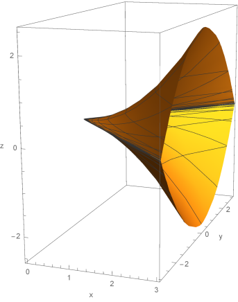
Figure 20: The Heisenberg beak $\partial\mathcal{A}$

Proof.

$(1)$, $(2)$ follow from item (2) of Th. 9 and item (3) of Sec. 4.

$(3)$ and $(6)$–$(8)$ are obvious.

$(4)$ follows from Th. 8.

$(5)$ follows from Th. 12. ∎

Lightlike maximizers filling $S(0)$ are shown in Fig. 22. Sub-Lorentzian spheres or radii 0, 1, 2, 3 are shown in Fig. 22.

Figure 21: Lightlike maximizers filling $S(0)$

Figure 22: Sub-Lorentzian spheres or radii 0, 1, 2, 3

Remark 11.

The spheres

$$S(1)=\left\{(x,y,z)\in M\mid x=\sqrt{y^{2}+f(z)},\ y,z\in{\mathbb{R}}\right\},$$

$$S(0)=\left\{(x,y,z)\in M\mid x=\sqrt{y^{2}+4|z|},\ y,z\in{\mathbb{R}}\right\}$$

tend one to another as $z\to\infty$ since for any $y\in{\mathbb{R}}$

$$\lim_{z\to\infty}\left(\sqrt{y^{2}+f(z)}-\sqrt{y^{2}+4|z|}\right)=0$$

by virtue of $(\ref{fas})$. The same holds for any spheres $S(R_{1})$, $S(R_{2})$, $R_{i}\in[0,+\infty)$.

11 Conclusion

The results obtained in this paper for the sub-Lorentzian problem on the Heisenberg group differ drastically from the known results for the sub-Riemannian problem on the same group:

1. The sub-Lorentzian problem is not completely controllable.

2. Filippov’s existence theorem for optimal controls cannot be immediately applied to the sub-Lorentzian problem.

3. In the sub-Lorentzian problem all extremal trajectories are infinitely optimal, thus the cut locus and the conjugate locus for them are empty.

4. The sub-Lorentzian length maximizers coming to the zero-radius sphere are nonsmooth (concatenations of two smooth arcs forming a corner, nonstrictly normal extremal trajectories).

5. Sub-Lorentzian spheres and sub-Lorentzian distance are real-analytic if $d>0$.

It would be interesting to understand which of these properties persist for more general sub-Lorentzian problems (e.g., for left-invariant problems on Carnot groups).

The authors thank A.A.Agrachev, L.V.Lokutsievskiy, and M. Grochowski for valuable discussions of the problem considered.

List of Figures

1. 1 The Heisenberg beak $\partial\mathcal{A}$
2. 4 Previously obtained results
3. Remark 2.
4. 6 Nonstrictly normal $(x(t),y(t))$
5. 5.2 Normal case
6. 6 Inversion of the exponential mapping
7. 11 Plot of $\frac{p}{\sinh p}$
8. 8 Sub-Lorentzian distance
9. 14 Plot of $\left.d\right|_{x=1}$
10. 15 Bound $(\ref{bound})$
11. 10.1 Spheres of positive radius
12. 10.1 Spheres of positive radius
13. 20 The Heisenberg beak $\partial\mathcal{A}$
14. 10.2 Sphere of zero radius

References

- [1] A.M. Vershik, V.Y. Gershkovich, Nonholonomic Dynamical Systems. Geometry of distributions and variational problems. (Russian) In: Itogi Nauki i Tekhniki: Sovremennye Problemy Matematiki, Fundamental’nyje Napravleniya, Vol. 16, VINITI, Moscow, 1987, 5–85. (English translation in: Encyclopedia of Math. Sci. 16, Dynamical Systems 7, Springer Verlag.)
- [2] V. Jurdjevic, Geometric Control Theory, Cambridge University Press, 1997.
- [3] R. Montgomery, A tour of subriemannian geometries, their geodesics and applications, Amer. Math. Soc., 2002.
- [4] A. Agrachev, Yu. Sachkov, Control theory from the geometric viewpoint, Berlin Heidelberg New York Tokyo. Springer-Verlag, 2004.
- [5] A. Agrachev, D. Barilari, U. Boscain, A Comprehensive Introduction to sub-Riemannian Geometry from Hamiltonian viewpoint, Cambridge University Press, 2019.
- [6] Yu. Sachkov, Introduction to geometric control, Springer, 2022.
- [7] Yu. Sachkov, Left-invariant optimal control problems on Lie groups: classification and problems integrable by elementary functions, Russian Math. Surveys, 77:1 (2022), 99–163
- [8] M. Grochowski, Geodesics in the sub-Lorentzian geometry. Bull. Polish. Acad. Sci. Math., 50 (2002).
- [9] M. Grochowski, Normal forms of germs of contact sub-Lorentzian structures on . Differentiability of the sub-Lorentzian distance. J. Dynam. Control Systems 9 (2003), No. 4.
- [10] M. Grochowski, Properties of reachable sets in the sub-Lorentzian geometry, J. Geom. Phys. 59(7) (2009) 885–900.
- [11] M. Grochowski, Reachable sets for contact sub-Lorentzian metrics on . Application to control affine systems with the scalar input, J. Math. Sci. (N.Y.) 177(3) (2011) 383–394.
- [12] M. Grochowski, On the Heisenberg sub-Lorentzian metric on , GEOMETRIC SINGULARITY THEORY, BANACH CENTER PUBLICATIONS, INSTITUTE OF MATHEMATICS, POLISH ACADEMY OF SCIENCES, WARSZAWA, vol. 65, 2004.
- [13] M. Grochowski, Reachable sets for the Heisenberg sub-Lorentzian structure on . An estimate for the distance function. Journal of Dynamical and Control Systems, vol. 12, 2006, 2, 145–160.
- [14] D.-C. Chang, I. Markina and A. Vasil’ev, Sub-Lorentzian geometry on anti-de Sitter space, J. Math. Pures Appl., 90 (2008), 82–110.
- [15] A. Korolko and I. Markina, Nonholonomic Lorentzian geometry on some H-type groups, J. Geom. Anal., 19 (2009), 864–889.
- [16] E. Grong, A. Vasil’ev, Sub-Riemannian and sub-Lorentzian geometry on and on its universal cover, J. Geom. Mech. 3(2) (2011) 225–260.
- [17] M. Grochowski, A. Medvedev, B. Warhurst, 3-dimensional left-invariant sub-Lorentzian contact structures, Differential Geometry and its Applications, 49 (2016) 142–166
- [18] H. Abels, E.B. Vinberg, On free two-step nilpotent Lie semigroups and inequalities between random variables, J. Lie Theory, 29:1 (2019), 79–87
- [19] L.S. Pontryagin, V. G. Boltyanskii, R. V. Gamkrelidze, E.F. Mishchenko, Mathematical Theory of Optimal Processes, New York/London. John Wiley & Sons, 1962.
- [20] E. Hakavuori, E. Le Donne, Non-minimality of corners in subriemannian geometry, Invent. Math., 206(3): 693–704, 2016.
- [21] L.V. Lokutsievskiy, A.V. Podobryaev, Existence of length maximizers in sub-Lorentzian problems on nilpotent Lie groups, in preparation.
- [22] A.Yu. Popov, Yu.L. Sachkov, Asymptotics of sub-Lorentzian distance at the Heisenberg group at the boundary of the attainable set, in preparation.