Systematic Review of Newton-Schulz Iterations with Unified Factorizations : Integration in the Richardson Method and Application to Robust Failure Detection in Electrical Networks

Abstract

Systematic overview of Newton-Schulz and Durand iterations with convergence analysis and factorizations is presented in the chronological sequence in unified framework. Practical recommendations for the choice of the order and factorizations of the algorithms and integration into Richardson iteration are given. The simplest combination of Newton-Schulz and Richardson iteration is applied to the parameter estimation problem associated with the failure detection via evaluation of the frequency content of the signals in electrical network. The detection is performed on real data for which the software failure was simulated, which resulted in the rank deficient information matrix. Robust preconditioning for rank deficient matrices is proposed and the efficiency of the approach is demonstrated by simulations via comparison with standard LU decomposition method.

1 Introduction

Parameter estimation problems appear often in adaptive control, [1],[2] system identification,[3], signal processing, [3] and in many other areas. Suppose that the process is described by the following equation:

$$y_{k}=\varphi_{k}^{T}\theta_{*}$$ (1)

where $\varphi_{k}$ is the regressor vector and $\theta_{*}$ is the vector of unknown parameters to be estimated, $k=1,2,...$
Introduction of the model in the form

$$\hat{y}_{k}=\varphi_{k}^{T}\theta_{k}$$ (2)

and minimization of the following function associated with the mismatch between the model and the process

$$E_{k}=\sum_{p=1}^{p=k}(\hat{y}_{p}-y_{p})^{2}$$ (3)

yields the following restricted linear system of equations :

$$A_{k}\theta_{k} =b_{k}$$ (4)

$$A_{k} =\sum_{p=1}^{p=k}\varphi_{p}\leavevmode\nobreak\ \varphi_{p}^{T},\leavevmode\nobreak\ b_{k}=\sum_{p=1}^{p=k}\varphi_{p}\leavevmode\nobreak\ y_{p}$$ (5)

which should be solved with respect to $\theta_{k}$. Accurate and computationally efficient solution of (4) is the most significant part of the estimation problem. The solution may benefit from the properties of the matrix $A_{k}$, which depend on the type of regressor and the step number associated with the window size. The matrix $A_{k}$ is SPD (Symmetric and Positive Definite) matrix in many cases. For example, the matrix $A$ is SPD for the systems with harmonic regressor, [1] - [5]. In general case the equation (4) can be multiplied by $A^{T}_{k}$ (for any invertible matrix $A_{k}$) that transforms the system to the SPD case with the Gram matrix, [6]. Notice that the Gram matrix is often ill-conditioned matrix due to squaring of the condition number [6].
The matrix $A$ is SPD ill-conditioned (a) information matrix for systems with harmonic regressor and short window sizes, [7],[8] (b) Gram matrix due to the squaring of the condition number in the least squares method, [3], [6], (c) mass matrix in finite element method, [9] and mass matrix (lumped mass matrix) for mechanical systems with singular perturbations, [10], (d) state matrix for systems of linear equations, [11] and in many other applications. Moreover, many processes in practice are singulary perturbed (have modes with different time-scales), [12] and considered as stiff and ill-conditioned systems, which potentially extends application areas of this model. In other words the model (4) with SPD (and possibly ill-conditioned matrix $A_{k}$) covers almost all the cases in the parameter estimation applications.
Ill-conditioning implies robustness problems (sensitivity to numerical calculations) and imposes additional requirements on the accuracy of the solution of (4) (which are especially pronounced in finite-digit calculations) since small changes in $b_{k}$ due to measurement, truncation, accumulation, rounding and other errors result in significant changes in $\theta_{k}$. In addition, ill-conditioning implies slow convergence of the iterative procedures.
The accuracy requirements is the main motivation for application of the Richardson iteration which is driven by the residual error and has filtering (averaging) property. The residual error is smoothed and remains bounded for a sufficiently large step number in this iteration, where the bound depends on inaccuracies, providing the best possible solution in finite digit calculations.
Therefore convergence rate improvement and reduction of the computational complexity of the Richardson iteration is one of the most important problems in the area. One of the ways to convergence rate improvement is introduction of the Newton-Schulz and Durand algorithms in the Richardson iteration, [8], [13] - [16].
This paper starts with short systematic overview (presented in unified tutorial fashion) of Newton-Schulz and Durand iterations in Section 2. Special attention is paid to practical introduction to power series factorizations for reduction of the computational complexity in Section 3. The simplest integration of Newton-Schulz algorithms in the Richardson iteration is presented in Section 4 with application to practical problem in Section 5. The problem is associated with the failure detection via estimation of the frequency content of the signals in electrical system in the presence of missing data. The detection is performed on real signals with simulated failure in the software. The efficiency of the approach is demonstrated in Section 5. The paper ends with brief conclusions in Section 6.

2 Overview of Iterative Matrix Inversion Algorithms:  Mini Tutorial

Brief overview of iterative matrix inversion algorithms with convergence analysis is presented in this Section. The overview is presented in the systematic way (from simple algorithms to more sophisticated ones) in the chronological sequence with convergence analysis and starts with the second order Newton-Schulz algorithms in Section 2.1 followed by the description of high order Newton-Schulz algorithms in Section 2.2. Computationally efficient Durand iterations are described in Section 2.3, and finally the combination for convergence rate improvement of high order Newton-Schulz and Durand algorithms is presented in Section 2.4.

2.1 Second Order Newton-Schulz Iterations

Consider the following iterations, [17] - [20]:

$$G_{k}=G_{k-1}+F_{k-1}G_{k-1},\leavevmode\nobreak\ \leavevmode\nobreak\ F_{k}=I-G_{k}A,$$ (6)

where $I$ is the identity matrix, $k=0,1,2...$ . Evaluation of the error in the first step $F_{1}$ yields :

$$F_{1} =I-(G_{0}+F_{0}\leavevmode\nobreak\ G_{0})\leavevmode\nobreak\ A=I-(I+F_{0})\leavevmode\nobreak\ G_{0}\leavevmode\nobreak\ A$$

$$=I-(I+F_{0})\leavevmode\nobreak\ (I-F_{0})=I-I^{2}+F_{0}^{2}=F_{0}^{2}$$

$$F_{2} =F_{1}^{2}=F_{0}^{4}$$

which gives the error model:

$$F_{k}=F_{0}^{2^{k}}$$ (7)

Algorithm (6) which is also known as Newton-Schulz-Hotelling matrix iteration, [18] estimates the inverse of the matrix $A$ via minimization of the estimation error $F_{k}$ provided that the spectral radius of initial matrix

$$\rho(F_{0})=\rho(I-G_{0}A)<1$$ (8)

is less than one, where $G_{0}$ is preconditioner (initial guess of $A^{-1}$). The proof of convergence is presented in [17] - [20], where the algorithm (6) is written in the following form: $G_{k}=G_{k-1}+G_{k-1}F_{k-1}$, where $F_{k}=I-AG_{k}$.
The order of the iterative algorithm can be increased for convergence rate improvement by introduction of the power series in the algorithm (6).

2.2 High Order Newton-Schulz Iterations

High order algorithms (which are also known as hyperpower iterative algorithms, which are widely used for calculation of generalized inverses) can be presented in the following form for $n=2,3,...$, [21] - [23] :

$$G_{k} =\sum_{j=0}^{n-1}F^{j}_{k-1}G_{k-1}=(I+F_{k-1}+F^{2}_{k-1}+...+F^{n-1}_{k-1})\leavevmode\nobreak\ G_{k-1}$$ (9)

or in the form presented in [16], [22] :

$$G_{k} =\sum_{j=0}^{n-1}F^{j}_{k-1}G_{k-1}=G_{k-1}+F_{k-1}\leavevmode\nobreak\ \sum_{j=0}^{n-2}F^{j}_{k-1}G_{k-1}$$ (10)

The error $F_{k}$ in (9) can be written in the following form:

$$F_{k} =I-G_{k}A=I-(I+F_{k-1}+F^{2}_{k-1}+...+F^{n-1}_{k-1})G_{k-1}A$$

$$=I-(I+F_{k-1}+F^{2}_{k-1}+...+F^{n-1}_{k-1})(I-F_{k-1})=F_{k-1}^{n}$$

$$F_{k} =F_{0}^{n^{k}}$$ (11)

Notice that the algorithm (9) is written in following form in [21] - [23] (and it is widely used in this form):

$$G_{k} =G_{k-1}\sum_{j=0}^{n-1}F^{j}_{k-1}=G_{k-1}(I+F_{k-1}+F^{2}_{k-1}+...+F^{n-1}_{k-1})$$ (12)

with $F_{k}=I-AG_{k}$. Notice that the error $F_{k}=I-G_{k}A$ is better aligned with Richardson iteration, see Section 4 and therefore is considered further in this paper.

2.3 Durand Iterations

Computationally efficient matrix inversion method described by Durand, [24], [25] can be derived from the relation associated with the initial error in Newton-Schulz approach,  $A^{-1}=F_{0}A^{-1}+G_{0}$ by substitution of $G_{k}$ instead of $A^{-1}$ as follows :

$$G_{k} =F_{0}\leavevmode\nobreak\ G_{k-1}+G_{0}$$ (13)

$$G_{k}-A^{-1} =F_{0}\leavevmode\nobreak\ (G_{k-1}-A^{-1})$$ (14)

$$F_{k} =I-G_{k}A=F^{k+1}_{0}$$ (15)

The error models (14), (15) are valid for the algorithm (13). Higher order Durand iterations are discussed in [8], [25].
Notice that the convergence rate of Newton-Schulz Iterations is significantly higher than the convergence rate of Durand iterations. However, Durand iteration (13) requires only one matrix product in each step.
Notice also that the convergence performance can be enhanced by introduction of the initial power series as preconditioning $G_{0}$ (which is calculated only once) in Newton-Schulz and Durand iterations, [8], [26]. The order of initial power series can be chosen sufficiently high, which essentially improves the convergence rate. Computational complexity of initial power series can be reduced via factorizations, see Section 3 for details.
Convergence rate can also be improved via combination of two Newton-Schulz iterations, which also cover Durand iterations as special case, see next Section 2.4.

2.4 Convergence Rate Improvement via Combination of High Order Newton-Schulz Iterations

Consider the following combination of two Newton-Schulz iterations associated with two-step iterative method, [27] :

$$\Gamma_{k} =I-L_{k-1}A$$ (16)

$$L_{k} =\{\sum_{j=0}^{n-1}\Gamma^{j}_{k}\}\leavevmode\nobreak\ L_{k-1}$$ (17)

$$\Gamma^{n}_{k} =I-L_{k}A$$ (18)

$$G_{k} =\underbrace{L_{k}}_{\begin{subarray}{l}\text{Newton-Schulz }\\ \text{Iteration }\end{subarray}}+\underbrace{\Gamma^{n}_{k}}_{\begin{subarray}{l}\text{High Order }\\ \text{Convergence}\\ \text{Accelerator}\end{subarray}}\leavevmode\nobreak\ \leavevmode\nobreak\ \underbrace{\{\sum_{j=0}^{n-1}F^{j}_{k-1}\}\leavevmode\nobreak\ G_{k-1}}_{\begin{subarray}{l}\text{Newton-Schulz }\\ \text{Iteration }\end{subarray}}$$ (19)

$$F_{k} =I-G_{k}A=\Gamma^{n}_{k}\leavevmode\nobreak\ F^{n}_{k-1}$$ (20)

$$F_{k} =F_{0}^{\displaystyle\leavevmode\nobreak\ k\leavevmode\nobreak\ n^{k+1}+\leavevmode\nobreak\ n^{k}},\leavevmode\nobreak\ \text{for}\leavevmode\nobreak\ n>1$$ (21)

where $\displaystyle L_{0}=\sum_{j=0}^{n-1}\Gamma^{j}_{0}\leavevmode\nobreak\ S^{-1}$,  $\Gamma_{0}=F_{0}=I-S^{-1}A$, where $\displaystyle G_{0}=S^{-1}$ satisfies (8). Notice that Durand iteration (13) can be derived from (16) - (19) with $n=1$. The error model (20) can be proved via multiplication of (19) by $A$ and explicit evaluation of the error $F_{k}$ (similar to Section 2.2, see also [21], [27]) as follows:

$$F_{k} =I-G_{k}A=\underbrace{I-L_{k}A}_{\Gamma^{n}_{k}}-\Gamma^{n}_{k}\sum_{j=0}^{n-1}F^{j}_{k-1}\underbrace{G_{k-1}A}_{I-F_{k-1}}=\Gamma^{n}_{k}\leavevmode\nobreak\ F^{n}_{k-1}$$ (22)

The error model (21) is obtained via explicit evaluation of (22). The algorithm (16) - (21) has two independent and equally complex computational parts: the first part is associated with calculations of $\Gamma_{k}$, $L_{k}$ and $\Gamma^{n}_{k}$, where $\Gamma_{k}=\Gamma^{n}_{k-1}$, whereas the term $\displaystyle\sum_{j=0}^{n-1}F^{j}_{k-1}G_{k-1}$ is calculated in the second part. This algorithm is ideally suited for parallel implementation.

Extended version of this survey is presented in Stotsky A., Recursive Versus Nonrecursive Richardson Algorithms: Systematic Overview, Unified Frameworks and Application to Electric Grid Power Quality Monitoring, Automatika, vol. 63, N2, pp. 328-337, 2022, https://doi.org/10.1080/00051144.2022.2039989, [33].

Further developments can be found in Stotsky A.,Simultaneous Frequency and Amplitude Estimation for Grid Quality Monitoring : New Partitioning with Memory Based Newton-Schulz Corrections, IFAC PapersOnLine 55-9, pp. 42-47, 2022, https://www.sciencedirect.com/science/article/pii/S2405896322003937 ,[34].

3 Reduction of Computational Complexity via Unified Factorizations

The following high order Newton-Schulz power series can be factorized for composite orders $n$ as follows, [27] :

$$G_{k} =\{\sum_{j=0}^{n-1}F_{k-1}^{j}\}\leavevmode\nobreak\ G_{k-1}=\{\sum_{j=0}^{w-1}F_{k-1}^{(p+1)j}\}\leavevmode\nobreak\ \{\sum_{d=0}^{p}F_{k-1}^{d}\}\leavevmode\nobreak\ G_{k-1}$$ (23)

$$F_{k-1}^{p+1} =I-\{\sum_{d=0}^{p}F_{k-1}^{d}\}\leavevmode\nobreak\ G_{k-1}\leavevmode\nobreak\ A$$

$$=I-\{\sum_{d=0}^{p}F_{k-1}^{d}\}\leavevmode\nobreak\ \{I-F_{k-1}\},\leavevmode\nobreak\ F_{k-1}=I-G_{k-1}A$$ (24)

$$n =w\leavevmode\nobreak\ (p+1),\leavevmode\nobreak\ \leavevmode\nobreak\ p=0,1,2,...,\leavevmode\nobreak\ w=1,2,3,...$$ (25)

Taking into account that every prime number is followed after the composite number the factorization for the prime orders $n+1$ can be performed as follows:

$$G_{k} =(I+F_{k-1}\{\sum_{j=0}^{w-1}F_{k-1}^{(p+1)j}\}\leavevmode\nobreak\ \{\sum_{d=0}^{p}F_{k-1}^{d}\})\leavevmode\nobreak\ G_{k-1}$$ (26)

$$=\{\sum_{j=0}^{(n+1)-1}F_{k-1}^{j}\}\leavevmode\nobreak\ G_{k-1}$$

Similar factorizations can be found in [28]. The following efficiency index introduced in [29] is widely used for quantification of the performance of different factorizations:

$$EI=\displaystyle n^{1/n_{p}}$$ (27)

where $n$ is the order of the algorithm and $n_{p}$ is the number of matrix products per each cycle. For illustration of the unified factorization approach few examples with increasing EI are presented below.

3.1 Case of $n=8=w\leavevmode\nobreak\ (p+1)$,  $p=3$, $w=2$

$$G_{k} =\{\sum_{j=0}^{1}F_{k-1}^{4j}\}\leavevmode\nobreak\ \{\sum_{d=0}^{3}F_{k-1}^{d}\}\leavevmode\nobreak\ G_{k-1}$$ (28)

$$=(I+F_{k-1}^{4})(I+F_{k-1}^{2})(I+F_{k-1})\leavevmode\nobreak\ G_{k-1}$$

which requires $6$ matrix products with $EI=1.4142$ .

3.2 Case of $n=9=w\leavevmode\nobreak\ (p+1)$,  $p=2$, $w=3$

$$G_{k} =\{\sum_{j=0}^{2}F_{k-1}^{3j}\}\leavevmode\nobreak\ \{\sum_{d=0}^{2}F_{k-1}^{d}\}\leavevmode\nobreak\ G_{k-1}$$

$$=(I+F_{k-1}^{3}+F_{k-1}^{6})(I+F_{k-1}+F_{k-1}^{2})\leavevmode\nobreak\ G_{k-1}$$

$$=(I+(I+F_{k-1}^{4})(I+F_{k-1}^{2})(F_{k-1}+F_{k-1}^{2}))\leavevmode\nobreak\ G_{k-1}$$

which requires $6$ matrix products with $EI=1.4422$ .

3.3 Case of $n=10=w\leavevmode\nobreak\ (p+1)$,  $p=1$, $w=5$

$$G_{k} =\{\sum_{j=0}^{4}F_{k-1}^{2j}\}\leavevmode\nobreak\ \{\sum_{d=0}^{1}F_{k-1}^{d}\}\leavevmode\nobreak\ G_{k-1}$$

$$=(I+(F_{k-1}^{2}+F_{k-1}^{4})(I+F_{k-1}^{4}))(I+F_{k-1}))\leavevmode\nobreak\ G_{k-1}$$

which requires $6$ matrix products with $EI=1.4678$ .

3.4 Case of $n=11=w\leavevmode\nobreak\ (p+1)+1$,  $p=1$, $w=5$

$$G_{k} =(I+F_{k-1}\{\sum_{j=0}^{4}F_{k-1}^{2j}\}\leavevmode\nobreak\ \{\sum_{d=0}^{1}F_{k-1}^{d}\})\leavevmode\nobreak\ G_{k-1}$$ (29)

$$=(I+F_{k-1}(I+(F_{k-1}^{2}+F_{k-1}^{4})(I+F_{k-1}^{4}))(I+F_{k-1}))\leavevmode\nobreak\ G_{k-1}$$

$$=(I+(I+(F_{k-1}^{2}+F_{k-1}^{4})(I+F_{k-1}^{4}))(F_{k-1}+F^{2}_{k-1}))\leavevmode\nobreak\ G_{k-1}$$

which requires $6$ matrix products, $EI=1.4913$, [30].
Notice that the idea of factorization is associated with Newton-Schulz method. Therefore Newton-Schulz algorithms of low orders (order two or three) being iterated for a number of steps can be applied instead of factorized Newton-Schulz iterations of higher orders for the sake of robustness and efficiency.
Notice that three steps of the second order Newton-Schulz iteration are equivalent to one step of eighth order iteration with $6$ matrix products, see (28). However, application of the eleventh order algorithm, see (29) and [30] requires also $6$ mmm and provides faster convergence than three steps of the second order Newton-Schulz iteration. This algorithm has also the highest efficiency index, $EI=1.4913$ among the algorithms presented above. Therefore the proper choice of the order and factorization that is made for each particular application should represent the trade-off between the robustness and convergence rate.

4 Richardson Iterations

Many practical problems can be associated with restricted linear system of equations:

$$A\theta_{*}=b$$ (30)

which should be solved for $\theta_{*}$. Richardson iteration is the most promising solution to this problem which provides the best possible accuracy in finite digit calculations. Despite the fact that the inverse of matrix $A$ is not required in order to find $\theta_{*}$ the approximate inverse essentially improves convergence rate of the Richardson iteration, [8], [13] - [16]. The simplest combination of matrix inversion techniques and Richardson algorithm can be presented as follows :

$$\theta_{k} =\theta_{k-1}-G_{k}\leavevmode\nobreak\ (A\theta_{k-1}-b)=F_{k-1}\theta_{k-1}+G_{k}b$$ (31)

where $\theta_{k}$ is the estimate of $\theta_{*}$,  $G_{k}$ is associated with the estimate of the inverse of $A$ and $F_{k}$ is the inversion error, see Section 2. Iteration (31) can be implemented using matrix vector products only.
Notice that definition of the inversion error in the form $F_{k}=I-G_{k}A$ is more convenient than the following definition $F_{k}=I-AG_{k}$ since the error $F_{k}=I-G_{k}A$ is better aligned with Richardson iteration providing the same convergence conditions. The convergence analysis of Richardson iteration with the error $F_{k}=I-AG_{k}$ can be found for example in [14].
Any matrix inversion algorithms presented in Section 2 with factorizations described in Section 3 can be applied in (31). Error models for different choices of $G_{k}$ are presented in [8]. Since $G_{k}$ is getting closer to $A^{-1}$ in each step the convergence rate of (31) is essentially improved. Updating of $G_{k}$ can even be stopped after several steps for reduction of the computational burden.

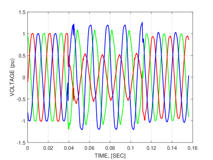
(a)

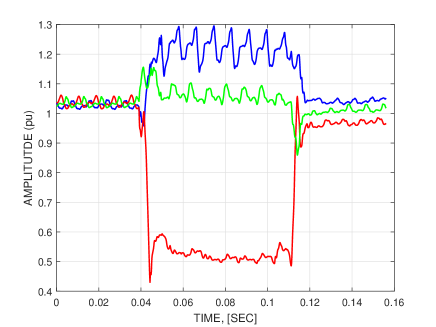
(b)

Figure 1: The voltages which correspond to the sag and swell events in phases ’a’,’b’ and ’c’ are plotted with green, red and blue lines respectively in Figure 1(a). The voltages are associated with the failure event with ID $2911$. The data is obtained from the DOE/EPRI National Database of Power System Events, [31]. The cause of this event is unknown. Amplitudes of the first harmonic (with the corresponding colours) which show delectability of the sag and swell events for the signals in Figure 1(a) are plotted in Figure 1(b). The detection is performed with rank deficient information matrix.

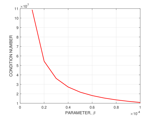
Figure 2: The condition number of the matrix $A_{rk}$ in (40) as a function of the regularization parameter $\beta>0$ is plotted. For a small $\beta$ the matrix $A_{rk}$ is ill-conditioned matrix for which the spectral radius $\displaystyle\rho(I-S_{k}^{-1}A_{rk})$, where $\displaystyle S_{k}^{-1}=I/\alpha_{k}$ with $\alpha_{k}=\|A_{rk}\|_{\infty}/2+\varepsilon$ is very close to one.

5 Estimation of the Frequency Content of Electrical Signals for Robust Failure Detection

Suppose that the measured electrical signal (voltage or current) $y_{k}$ can be presented in the following form

$$y_{k}=\varphi_{k}^{T}\vartheta+\xi_{k}$$ (32)

where $\vartheta$ is the vector of unknown constant parameters and $\varphi_{k}$ is the harmonic regressor presented in the following form:

$$\varphi_{k}^{T}=[\cos(q_{0}k)\leavevmode\nobreak\ \sin(q_{0}k)\leavevmode\nobreak\ \cos(2q_{0}k)$$

$$\leavevmode\nobreak\ \sin(2q_{0}k)\leavevmode\nobreak\ ...\leavevmode\nobreak\ \cos(mq_{0}k)\leavevmode\nobreak\ \sin(mq_{0}k)]$$ (33)

where $q_{0}$ is the fundamental frequency of network (for example $q_{0}=50$ Hertz or $q_{0}=60$ Hertz), $m$ is the number of harmonics, and $\xi_{k}$ is a zero mean white Gaussian noise, $k=1,2,...$ is the step number.
The model of the signal (32) with adjustable parameters $\theta_{*k}$ is presented in the following form:

$$\hat{y}_{k}=\varphi_{k}^{T}\theta_{*k}$$ (34)

The signal $y_{k}$ is approximated by the model $\hat{y}_{k}$ in the least squares sense in each step $k$ of moving window of a size $s$.
The estimation algorithm is based on minimization of the following error $E_{k}$;

$$E_{k}=\sum_{p=k-(s-1)}^{p=k}(\hat{y}_{p}-y_{p})^{2}$$ (35)

for a fixed step $k$, where $k\geq s$.
The least squares solution for estimation of the parameter vector $\theta_{*k}$, which should be calculated in each step can be written as follows:

$$A_{k}\theta_{*k} = b_{k}$$ (36)

$$A_{k} = \sum_{p=k-(s-1)}^{p=k}\varphi_{p}\leavevmode\nobreak\ \varphi_{p}^{T}$$ (37)

$$b_{k} = \sum_{p=k-(s-1)}^{p=k}\varphi_{p}\leavevmode\nobreak\ y_{p}$$ (38)

5.1 Missing Input Data & Rank Deficiency of Information Matrix

The matrix $A_{k}$ is symmetric and positive definite information matrix for systems with harmonic regressor for a sufficiently large window size $s$. However, the software, functional or system failures may occur, which usually result in declaration of zero values in the information matrix $A_{k}$. Such failures may result in rank deficiency of the information matrix $A_{k}$ in each step. Nevertheless, the methods described above can be still applied in this case.

5.2 Fault Detection on Real Data

Power quality monitoring and detection of sag and swell events is considered in the presence of system failures. Monitoring is performed via estimation of the frequency content of the voltage signals in three phase system. Real data obtained from the DOE/EPRI National Database of Power System Events, [31] is used for power quality monitoring. The event (Event ID $2911$) which resulted in voltage sag and swell was considered. The cause of this event is unknown and the event is considered as temporary fault. Measured voltage signals which correspond to the sag and swell in phases ’a’,’b’ and ’c’ are plotted with green, red and blue lines respectively in Figure 1(a).
It is assumed that the voltage signals can be described by the model (32) with harmonic regressor (33) and fundamental frequency of $60$ Hertz with four higher harmonics and unknown parameter vector $\vartheta$. The model of the signals is given by (34) with the vector of the parameters $\theta_{*k}$ which estimates unknown vector $\vartheta$. The estimation problem is reduced to the restricted linear system of equations (36) which should be solved w.r.t. $\theta_{*k}$ in each step. The $10\leavevmode\nobreak\ \times\leavevmode\nobreak\ 10$ matrix $A_{k}$ is the SPD matrix in each step (which is verified by simulations).
Suppose that a functional or system failure occurred, which resulted in three zero columns (columns 3,4 and 5) of the information matrix $A_{k}$ in each step.
In addition, suppose that three components of the vector $b_{k}$ (the components 3,4 and 5) are zeros in each step due to similar failure. Such failures result in rank deficient information matrix $A_{k}$ in each step. The rank of the information matrix is equal to seven in this case. Nevertheless, the methods described above can be applied in this case.

5.3 Pre-Conditioning for Rank Deficient Information Matrix

In order to apply the methods described above the matrix $S_{k}^{-1}$ should be chosen such that the spectral radius of the matrix $\displaystyle I-S_{k}^{-1}A_{k}$ is less than one in each step, $\displaystyle\rho(I-S_{k}^{-1}A_{k})<1$. For SPD information matrices the pre-conditioner can be chosen as $\displaystyle S_{k}^{-1}=I/\alpha_{k}$ with $\alpha_{k}=\|A_{k}\|_{\infty}/2+\varepsilon$, where $\|\cdot\|_{\infty}$ is the maximum row sum matrix norm, $\varepsilon>0$, [7], [32]. In the case of software or system failures the information matrix may become rank deficient and special preconditioning should be applied. Consider the following transformation of the system (36) and regularization of the matrix $A_{k}$:

$$A_{rk}\theta_{*k} =A^{T}_{k}b_{k}$$ (39)

$$A_{rk} =\beta I+A^{T}_{k}A_{k}$$ (40)

where $\beta$ is a small positive number, and the matrix $A_{rk}$ is SPD matrix for which the preconditioning described above can be applied. The choice of the parameter $\beta$ represents the trade-off between high condition number (for very small $\beta$) and the performance of regularization and hence the performance of the event detection (for large $\beta$). The condition number of $A_{rk}$ as a function of the regularization parameter $\beta$ is shown in Figure 2. For a small $\beta$ which allows high performance detection the matrix $A_{rk}$ becomes ill-conditioned matrix (which is sensitive to numerical operations) for which the spectral radius $\displaystyle\rho(I-S_{k}^{-1}A_{rk})$ is very close to one. Application of the stepwise splitting method, where the matrix $A$ is split recursively in each step provides robust solution for ill-conditioned case, [32].
Notice that the model (39), (40) provides robust solution for parameter estimation problems in the case of insufficient excitation and singular information matrices and can be applied instead of classical self-tuning adaptive and estimation algorithms in adaptive control and system identification, [1] - [3].

5.4 Simulation Results

Amplitudes of the first harmonic of the measured signals recovered by the Richardson parameter estimation algorithm (31) with the second order matrix inversion method (6) are presented in Figure 1(b). The Figure shows that the sag and swell events are detectable using the approach described above even in the presence of system failures, which result in rank deficiency of information matrix. The estimation accuracy was evaluated as the average sum of squares of the parameter errors for Richardson algorithm with respect to parameter vector calculated without missing data. The parameter vector calculated with Richardson algorithm is quite close to the parameter vector calculated without missing data.
In addition, LU decomposition method was also applied for parameter calculation in (36) with regularized matrix $A_{rk}$, which is close to singular matrix (extremely ill-conditioned) for sufficiently small $\beta$. LU decomposition method is very sensitive to numerical errors for extremely ill-conditioned matrices, whereas Richardson algorithm delivers robust solution. Therefore Richardson algorithms are recommended for robust detection of the failure events in the presence of missing data.

6 CONCLUSIONS

The practical guide for solution of the parameter estimation problem described by restricted linear system of equations was presented in the Richardson framework, which provides the best possible solution in finite digit calculations. Newton-Schulz and Durand iterations with unified factorizations, which enhance the performance of the Richardson method are presented in the form of tutorial (in historical framework) with the convergence analysis.
The combination of Richardson method with second order Newton-Schulz approach was tested in the failure detection problem on real signals from the electrical network. In addition, the software or system failure was simulated which resulted in rank deficiency of the information matrix. New preconditioning method was proposed for rank deficient matrices in the problem of estimation of the frequency contents of electrical signals. It was shown that the Richardson method is applicable in the failure detection problems with rank deficient information matrices.

References

- [1] Fomin V., Fradkov A. and Yakubovich V., Adaptive Control of Dynamic Objects, Nauka, Moscow, 1981 (in Russian).
- [2] Ioannou P. and Sun J., Robust Adaptive Control, Prentice Hall, Upper Saddle River, NJ, 1996.
- [3] Ljung L., System Identification: Theory for the User, Prentice-Hall, Upper Saddle River, NJ, 1999.
- [4] Bayard, D., A General Theory of Linear Time-Invariant Adaptive Feedforward Systems with Harmonic Regressors. IEEE Trans. Autom. Control vol. 45, N 11, pp. 1983-1996, 2000.
- [5] Stotsky A., Recursive Trigonometric Interpolation Algorithms, Journal of Systems and Control Engineering, vol. 224, N 1, pp. 65-77, 2010.
- [6] Björck Å., Numerical Methods for Least Squares Problems, SIAM, First edition, April 1, 1996.
- [7] Stotsky A., Accuracy Improvement in Least-Squares Estimation with Harmonic Regressor: New Preconditioning and Correction Methods, 54-th CDC, Dec. 15-18, Osaka, Japan, 2015, pp. 4035-4040.
- [8] Stotsky A., Unified Frameworks for High Order Newton-Schulz and Richardson Iterations: A Computationally Efficient Toolkit for Convergence Rate Improvement, Journal of Applied Mathematics and Computing, vol. 60, N 1 - 2, pp. 605-623, 2019.
- [9] Sticko S., Towards Higher Order Immersed Finite Elements for the Wave Equation, IT Licentiate theses, 2016-008, Uppsala University, Department of Information Technology, 2016.
- [10] Moustafa K., Real-Time Identification of Ill-Conditioned Structures, Journal of Offshore Mechanics and Arctic Engineering, August, vol. 112, pp. 181 - 186, 1990.
- [11] Hasan A., Kerrigan E. , Constantinides G., Solving a Positive Definite System of Linear Equations via the Matrix Exponential, 50-th IEEE CDC-ECC, Orlando, FL, USA, December 12-15, 2011, pp. 2299-2304.
- [12] Kokotovic P., Applications of Singular Perturbation Techniques to Control Problems, SIAM Review, vol. 26, N 4, pp. 501-550, 1984.
- [13] Dubois D., Greenbaum A. and Rodrigue G., Approximating the Inverse of a Matrix for Use in Iterative Algorithms on Vector Processors, Computing, 22, pp. 257-268, 1979.
- [14] Srivastava S., Stanimirovic P., Katsikis V. and Gupta D., A Family of Iterative Methods with Accelerated Convergence for Restricted Linear System of Equations, Mediterr. J. Math., vol. 14-222, pp. 1-26, 2017.
- [15] Liu X., Du W., Yu Y. and Yonghui Qin Y., Efficient Iterative Method for Solving the General Restricted Linear Equation, Journal of Applied Mathematics and Physics, N 6, pp. 418-428, 2018.
- [16] Stotsky A., Combined High-Order Algorithms in Robust Least-Squares Estimation with Harmonic Regressor and Strictly Diagonally Dominant Information Matrix, Proc. IMechE Part I: Journal of Systems and Control Engineering, vol. 229, N 2, pp. 184-190, 2015.
- [17] Schulz G., Iterative Berechnung Der Reziproken Matrix, Zeitschrift für Angewandte Mathematik und Mechanik, vol. 13, pp. 57-59, 1933.
- [18] Hotelling H., Some New Methods in Matrix Calculation, Annals of Math. Stat., vol. 14, pp. 1-34, 1943.
- [19] Demidovich B., Maron I., Basics of Numerical Mathematics, Moscow, Fizmatgiz, 1963, (in Russian).
- [20] Ben-Israel A. , A Note on an Iterative Method for Generalized Inversion of Matrices, Math. Comput. vol. 20, pp. 439-440, 1966.
- [21] Isaacson E. and Keller H., Analysis of Numerical Methods, John Wiley & Sons, New York, 1966.
- [22] Petryshyn W., On Generalized Inverses and on the Uniform Convergence of with Application to Iterative Methods, J. Math. Anal. Appl., vol. 18, pp. 417-439, 1967.
- [23] Stickel E., On a Class of High Order Methods for Inverting Matrices, ZAMM Z. Angew. Math. Mech. 67, pp. 331-386, 1987.
- [24] Durand E., Solutions Numeriques des Equations Algebriques, vol. 2., Paris, Masson, 1972.
- [25] Brezinski C. Variations on Richardson’s Method and Acceleration, in: Numerical Analysis, A Numerical Analysis Conference in Honour of Jean Meinguet, Bull. Soc. Math. Belgium, 1996, pp. 33-44.
- [26] O’Leary, D., Yet Another Polynomial Preconditioner for the Conjugate Gradient Algorithm, Linear Algebra Appl. vol. 154-156, pp.377-388, 1991.
- [27] Stotsky A. , Efficient Iterative Solvers in the Least Squares Method, Proc. of the 21-st IFAC World Congress, Berlin, Germany, July 12-17,2020, pp. 901-906, see also arXiv:2008.11480v1 [math.OC], 26 Aug 2020.
- [28] Soleymani, F., Stanimirovic, P., Haghani, F., On Hyperpower Family of Iterations for Computing Outer Inverses Possessing High Efficiencies, Linear Algebra Appl., vol. 484,pp. 477-495, 2015.
- [29] Ehrmann H., Konstruktion und Durchführung von Iterationsverfahren höherer Ordnung. Arch. Ration. Mech. Anal., N. 4, pp. 65-88,1959.
- [30] Stanimirovic P., Kumar A. and Katsikis V., Further Efficient Hyperpower Iterative methods for the Computation of Generalized Inverses , RACSAM, vol.113, pp. 3323-3339, 2019.
- [31] DOE/EPRI National Database Repository of Power System Events.
- [32] Stotsky A., Grid Frequency Estimation Using Multiple Model with Harmonic Regressor: Robustness Enhancement with Stepwise Splitting Method, IFAC PapersOnLine 50-1, pp. 12817 - 12822, 2017.
- [33] Stotsky A. (2022). Recursive Versus Nonrecursive Richardson Algorithms: Systematic Overview, Unified Frameworks and Application to Electric Grid Power Quality Monitoring, Automatika, vol. 63, N2, pp. 328-337, https://doi.org/10.1080/00051144.2022.2039989
- [34] Stotsky A.,Simultaneous Frequency and Amplitude Estimation for Grid Quality Monitoring : New Partitioning with Memory Based Newton-Schulz Corrections, IFAC PapersOnLine 55-9, pp. 42-47, 2022, https://www.sciencedirect.com/science/article/pii/S2405896322003937