Neural Set Function Extensions:
Learning with Discrete Functions in High Dimensions

Abstract

Integrating functions on discrete domains into neural networks is key to developing their capability to reason about discrete objects. But, discrete domains are (I) not naturally amenable to gradient-based optimization, and (II) incompatible with deep learning architectures that rely on representations in high-dimensional vector spaces. In this work, we address both difficulties for set functions, which capture many important discrete problems. First, we develop a framework for extending set functions onto low-dimensional continuous domains, where many extensions are naturally defined. Our framework subsumes many well-known extensions as special cases. Second, to avoid undesirable low-dimensional neural network bottlenecks, we convert low-dimensional extensions into representations in high-dimensional spaces, taking inspiration from the success of semidefinite programs for combinatorial optimization. Empirically, we observe benefits of our extensions for unsupervised neural combinatorial optimization, in particular with high-dimensional representations.

1 Introduction

While neural networks are highly effective at solving tasks grounded in basic perception (Chen et al., 2020; Vaswani et al., 2017), discrete algorithmic and combinatorial tasks such as partitioning graphs, and finding optimal routes or shortest paths have proven more challenging. This is, in part, due to the difficulty of integrating discrete operations into neural network architectures (Battaglia et al., 2018; Bengio et al., 2021; Cappart et al., 2021a). One immediate difficulty with functions on discrete spaces is that they are not amenable to standard gradient-based training. Another is that discrete functions are typically expressed in terms of scalar (e.g., Boolean) variables for each item (e.g., node, edge to be selected), in contrast to the high-dimensional and continuous nature of neural networks’ internal representations. A natural approach to addressing these challenges is to carefully choose a function on a continuous domain that extends the discrete function, and can be used as a drop-in replacement.

There are several important desiderata that such an extension should satisfy in order to be suited to neural network training. First, an extension should be valid, i.e., agree with the discrete function on discrete points. It should also be amenable to gradient-based optimization, and should avoid introducing spurious minima. Beyond these requirements, there is one additional critical consideration. In both machine learning and optimization, it has been observed that high-dimensional representations can make problems “easier”. For instance, neural networks rely on high-dimensional internal representations for representational power and to allow information to flow through gradients, and performance suffers considerably when undesirable low-dimensional bottlenecks are introduced into network architectures (Belkin et al., 2019; Veličković & Blundell, 2021). In optimization, lifting to higher-dimensional spaces can make the problem more well-behaved (Goemans & Williamson, 1995; Shawe-Taylor et al., 2004; Du et al., 2018). Therefore, extending discrete functions to high-dimensional domains may be critical to the effectiveness of the resulting learning process, yet remains largely an open problem.

With those considerations in mind, we propose a framework for constructing extensions of discrete set functions onto high-dimensional continuous spaces. The core idea is to view a continuous point $\mathbf{x}$ in space as an expectation over a distribution (that depends on $\mathbf{x}$) supported on a few carefully chosen discrete points, to retain tractability. To evaluate the discrete function at $\mathbf{x}$, we compute the expected value of the set function over this distribution. The method resulting from a principled formalization of this idea is computationally efficient and addresses the key challenges of building continuous extensions. Namely, our extensions allow gradient-based optimization and address the dimensionality concerns, allowing any function on sets to be used as a computation step in a neural network.

First, to enable gradient computations, we present a method based on a linear programming (LP) relaxation for constructing extensions on continuous domains where exact gradients can be computed using standard automatic differentiation software (Abadi et al., 2016; Bastien et al., 2012; Paszke et al., 2019). Our approach allows task-specific considerations (e.g., a cardinalilty constraint) to be built into the extension design. While our initial LP formulation handles gradients, and is a natural formulation for explicitly building extensions, it replaces discrete Booleans with scalars in the unit interval $[0,1]$, and hence does not yet address potential dimensionality bottlenecks. Second, to enable higher-dimensional representations, we take inspiration from classical SDP relaxations, such as the celebrated Goemans-Williamson maximum cut algorithm (Goemans & Williamson, 1995), which recast low-dimensional problems in high-dimensions. Specifically, our key contribution is to develop an SDP analog of our original LP formulation, and show how to lift LP-based extensions into a corresponding high-dimensional SDP-based extensions. Our general procedure for lifting low-dimensional representations into higher dimensions aligns with the neural algorithmic reasoning blueprint (Veličković & Blundell, 2021), and suggests that classical techniques such as SDPs may be effective tools for combining deep learning with algorithmic processes more generally.

2 Problem Setup

Consider a ground set $[n]=\{1,\ldots,n\}$ and an arbitrary function $f\mathrel{\mathop{\mathchar 58\relax}}2^{[n]}\rightarrow\mathbb{R}\cup\{\infty\}$ defined on subsets of $[n]$. For instance, $f$ could determine if a set of nodes or edges in a graph has some structural property, such as being a path, tree, clique, or independent set (Bello et al., 2016; Cappart et al., 2021a). Our aim is to build neural networks that use such discrete functions $f$ as an intermediate layer or loss. In order to produce a model that is trainable using standard auto-differentiation software, we consider a continuous domain $\mathcal{X}$ onto which we would like to extend $f$, with sets embedded into $\mathcal{X}$ via an injective map $e\mathrel{\mathop{\mathchar 58\relax}}2^{[n]}\rightarrow\mathcal{X}$. For instance, when $\mathcal{X}=[0,1]^{n}$ we may take $e(S)=\mathbf{1}_{S}$, the Boolean vector whose $i$th entry is $1$ if $i\in S$, and $0$ otherwise. Our approach is to design an extension

$$\mathfrak{F}\mathrel{\mathop{\mathchar 58\relax}}\mathcal{X}\rightarrow\mathbb{R}$$

of $f$ and consider the neural network $\text{NN}_{2}\circ\mathfrak{F}\circ\text{NN}_{1}$ (if $f$ is used as a loss, $\text{NN}_{2}$ is simply the identity). To ensure that the extension is valid and amenable to automatic differentiation, we require that 1) it agrees with $f$ on all discrete points: $\mathfrak{F}(e(S))=f(S)\ \text{for all}\ S\subseteq[n]\ \text{with}\ f(S)<\infty$, and 2) $\mathfrak{F}$ is continuous.

There is a rich existing literature on extensions of functions on discrete domains, particularly in the context of discrete optimization (Lovász, 1983; Grötschel et al., 1981; Calinescu et al., 2011; Vondrák, 2008; Bach, 2019; Obozinski & Bach, 2012; Tawarmalani & Sahinidis, 2002). These works provide promising tools to reach our goal of neural network training. Building on these, our method is the first to use semi-definite programming (SDP) to combine neural networks with set functions. There are, however, different considerations in the neural network setting as compared to optimization. The optimization literature often focuses on a class of set functions and aims to build extensions with desirable optimization properties, particularly convexity. We do not focus on convexity, aiming instead to develop a formalism that is as flexible as possible. Doing so maximizes the applicability of our method, and allows extensions adapted to task-specific desiderata (see Section 3.1).

3 Scalar Set Function Extensions

We start by presenting a general framework for extending set functions onto $\mathcal{X}=[0,1]^{n}$, where a set $S\subseteq[n]$ is viewed as the Boolean indicator vector $e(S)=\mathbf{1}_{S}\in\{0,1\}^{n}$ whose $i$th entry is $1$ if $i\in S$ and $0$ otherwise. We call extensions onto $[0,1]^{n}$ scalar since each item $i$ is represented by a single scalar value—the $i$th coordinate of $\mathbf{x}\in\mathcal{X}$. These scalar extensions will become the core building blocks in developing high-dimensional extensions in Section 4.

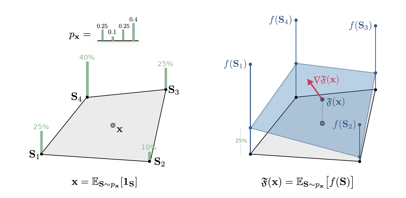
Figure 1: SFEs: Fractional points $\mathbf{x}$ are reinterpreted as expectations $\mathbf{x}=\mathbb{E}_{S\sim p_{\mathbf{x}}}[\mathbf{1}_{S}]$ over the distribution $p_{\mathbf{x}}(S)$ on sets. A value is assigned at $\mathbf{x}$ by exchanging the order of $f$ and the expectation: $\mathfrak{F}(\mathbf{x})_{S\sim p_{\mathbf{x}}}[f(S)]$. Unlike $f$, the extension $\mathfrak{F}$ is amenable to gradient-based optimization.

A classical approach to extending discrete functions on sets represented as Boolean indicator vectors $\mathbf{1}_{S}$ is by computing the convex-envelope, i.e., the point-wise supremum over linear functions that lower bound $f$ (Falk & Hoffman, 1976; Bach, 2019). Doing so yields a convex function whose value at a point $\mathbf{x}\in[0,1]^{n}$ is the solution of the following linear program (LP):

$$\widetilde{\mathfrak{F}}(\mathbf{x})=\underset{\mathbf{z},b\in\mathbb{R}^{n}\times\mathbb{R}}{\max}\{\mathbf{x}^{\top}\mathbf{z}+b\}\ \text{ subject to }\ \mathbf{1}_{S}^{\top}\mathbf{z}+b\leq f(S)\ \text{ for all }S\subseteq[n].$$ (primal LP)

The set $\mathcal{P}_{f}$ of all feasible solutions $(\mathbf{z},b)$ is known as the (canonical) polyhedron of $f$ (Obozinski & Bach, 2012) and can be seen to be non-empty by taking the coordinates of $\mathbf{z}$ to be sufficiently small (possibly negative). Variants of this optimization program are frequently encountered in the theory of matroids and submodular functions (Edmonds, 2003) where $\mathcal{P}_{f}$ is commonly known as the submodular polyhedron (see Appendix A for an extended discussion). By strong duality, we may solve the primal LP by instead solving its dual:

$$\widetilde{\mathfrak{F}}(\mathbf{x})=\underset{\{y_{S}\geq 0\}_{S\subseteq[n]}}{\min}\sum_{S\subseteq[n]}y_{S}f(S)\text{ subject to }\sum_{S\subseteq[n]}y_{S}\mathbf{1}_{S}=\mathbf{x},\ \sum_{S\subseteq[n]}y_{S}=1,\ \text{ for all }S\subseteq[n],$$ (dual LP)

whose optimal value is the same as the primal LP. The dual LP is always feasible (see e.g., the Lovász extension in Section 3.1). However, $\widetilde{\mathfrak{F}}$ does not necessarily agree with $f$ on discrete points in general, unless the function is convex-extensible (Murota, 1998).

To address this important missing piece, we relax our goal from solving the dual LP to instead seeking a feasible solution to the dual LP that is an extension of $f$. Since the dual LP is defined for a fixed $\mathbf{x}$, a feasible solution must be a function $y_{S}=p_{\mathbf{x}}(S)$ of $\mathbf{x}$. If $p_{\mathbf{x}}$ were to be continuous and a.e. differentiable in $\mathbf{x}$ then the value $\sum_{S}p_{\mathbf{x}}(S)f(S)$ attained by the dual LP would also be continuous and a.e. differentiable in $\mathbf{x}$ since gradients flow through the coefficients $y_{S}=p_{\mathbf{x}}(S)$, while $f(S)$ is treated as a constant in $\mathbf{x}$. This leads us to the following definition:

Definition (Scalar SFE).

A scalar SFE $\mathfrak{F}$ of $f$ is defined at a point $\mathbf{x}\in[0,1]^{n}$ by coefficients $p_{\mathbf{x}}(S)$ such that $y_{S}=p_{\mathbf{x}}(S)$ is a feasible solution to the dual LP. The extension value is given by

$$\mathfrak{F}(\mathbf{x})\triangleq\sum_{S\subseteq[n]}p_{\mathbf{x}}(S)f(S)$$

and we require the following properties to hold for all $S\subseteq[n]$: 1) $p_{\mathbf{x}}(S)$ is a continuous function of $\mathbf{x}$ and 2) $\mathfrak{F}(\mathbf{1}_{S})=f(S)$ for all $S\subseteq[n]$.

Efficient evaluation of $\mathfrak{F}$ requires that $p_{\mathbf{x}}(S)$ is supported on a small collection of carefully chosen sets $S$. This choice is a key inductive bias of the extension, and Section 3.1 gives many examples with only $O(n)$ non-zero coefficients. Examples include well-known extensions, such as the Lovász extension, as well as a number of novel extensions, illustrating the versatility of the SFE framework.

Thanks to the constraint $\sum_{S}y_{S}=1$ in the dual LP, scalar SFEs have a natural probabilistic interpretation. An SFE is defined by a probability distribution $p_{\mathbf{x}}$ such that fractional points $\mathbf{x}$ can be written as an expectation $\mathbb{E}_{S\sim p_{\mathbf{x}}}[\mathbf{1}_{S}]=\mathbf{x}$ over discrete points using $p_{\mathbf{x}}$. The extension itself can be viewed as arising from exchanging $f$ and the expectation operation: $\mathfrak{F}(\mathbf{x})=\mathbb{E}_{S\sim p_{\mathbf{x}}}[f(S)]$. This interpretation is summarized in Figure 1.

Scalar SFEs also enjoy the property of not introducing any spurious minima. That is, the minima of $\mathfrak{F}$ coincide with the minima of $f$ up to convex combinations. This property is especially important when training models of the form $f\circ\text{NN}_{1}$ (i.e., $f$ is a loss function) since $\mathfrak{F}$ will guide the network $\text{NN}_{1}$ towards the same solutions as $f$.

Proposition 1 (Scalar SFEs have no bad minima).

If $\mathfrak{F}$ is a scalar SFE of $f$ then:

1. $\min_{\mathbf{x}\in\mathcal{X}}\mathfrak{F}(\mathbf{x})=\min_{S\subseteq[n]}f(S)$

2. $\operatorname*{arg\,min}_{\mathbf{x}\in\mathcal{X}}\mathfrak{F}(\mathbf{x})\subseteq\text{Hull}\big{(}\operatorname*{arg\,min}_{\mathbf{1}_{S}\mathrel{\mathop{\mathchar 58\relax}}S\subseteq[n]}f(S)\big{)}$

See Appendix B for proofs.

Obtaining set solutions. Given an architecture $\mathfrak{F}\circ\text{NN}_{1}$ and input problem instance $G$, we often wish to produce sets as outputs at inference time. To do this, we simply compute $\mathbf{x}=\text{NN}_{1}(G)$, and select the set $S$ in $\text{supp}_{S}\{p_{\mathbf{x}}(S)\}$ with the smallest value $f(S)$. This can be done efficiently if, as is typically the case, the cardinality of $\text{supp}_{S}\{p_{\mathbf{x}}(S)\}$ is small.

3.1 Constructing Scalar Set Function Extensions

A key characteristic of scalar SFEs is that there are many potential extensions of any given $f$. In this section, we provide examples of scalar SFEs, illustrating the capacity of the SFE framework for building knowledge about $f$ into the extension. See Appendix C for all proofs and further discussion.

Lovász extension. Re-indexing the coordinates of $\mathbf{x}$ so that $x_{1}\geq x_{2}\ldots\geq x_{n}$, we define $p_{\mathbf{x}}$ to be supported on the sets $S_{1}\subseteq S_{2}\subseteq\dots\subseteq S_{n}$ with $S_{i}=\{1,2,\dots,i\}$ for $i=1,2,\dots,n$. The coefficient are defined as $y_{S_{i}}=p_{\mathbf{x}}(S_{i})\mathrel{\mathop{\mathchar 58\relax}}=x_{i}-x_{i+1}$ and $p_{\mathbf{x}}(S)=0$ for all other sets. The resulting Lovász extension—known as the Choquet integral in decision theory (Choquet, 1954; Marichal, 2000)—is a key tool in combinatorial optimization due to a seminal result: the Lovász extension is convex if and only if $f$ is submodular (Lovász, 1983), implying that submodular minimization can be solved in polynomial-time (Grötschel et al., 1981).

Bounded cardinality Lovász extension. A collection $\{S_{i}\}_{i=1}^{n}$ of subsets of $[n]$ can be encoded in an $n\times n$ matrix $\mathbf{S}\in\{0,1\}^{n\times n}$ whose $i$th column is $\mathbf{1}_{S_{i}}$. In this notation, the dual LP constraint $\sum_{S\subseteq[n]}y_{S}\mathbf{1}_{S}=\mathbf{x}$ can be written as $\mathbf{S}\mathbf{p}=\mathbf{x}$, where the $i$th coordinate of $\mathbf{p}$ defines $p_{\mathbf{x}}(S_{i})$. The bounded cardinality extension generalizes the Lovász extension to focus only on sets of cardinality at most $k\leq n$. Again, re-index $\mathbf{x}$ so that $x_{1}\geq x_{2}\ldots\geq x_{n}$. Use the first $k$ sets $S_{1}\subseteq S_{2}\subseteq\dots\subseteq S_{k}$, where $S_{i}=\{1,2,\dots,i\}$, to populate the first $k$ columns of matrix $\mathbf{S}$. We add further $n-k$ sets: $S_{k+i}=\{j+i\;|\;j\in S_{k}\}$ for $i=1,\dots,n-k$, to fill the rest of $\mathbf{S}$. Finally, $p_{\mathbf{x}}(S_{i})$ can be analytically calculated from $\mathbf{p}=\mathbf{S}^{-1}\mathbf{x}$, where $\mathbf{S}$ is invertible since it is a Toeplitz banded upper triangular matrix.

Permutations and involutory extensions. We use the same $\mathbf{S},\mathbf{p}$ notation. Let $\mathbf{S}$ be an elementary permutation matrix. Then it is involutory, i.e., $\mathbf{S}\mathbf{S}=\mathbf{I}$, and we may easily determine $\mathbf{p}=\mathbf{S}\mathbf{x}$ given $\mathbf{S}$ and $\mathbf{x}$. Note that $p_{\mathbf{x}}(S_{i})=\mathbf{p}_{i}$ must be non-negative since $\mathbf{x}$ and $\mathbf{S}$ are non-negative entry-wise. Finally, restricting $\mathbf{x}$ to the $n$-dimensional Simplex guarantees that $\|\mathbf{p}\|_{1}\leq 1$, which ensures $p_{\mathbf{x}}$ is a probability distribution (any remaining mass is placed on the empty set). The extension property can be guaranteed on singleton sets as long as the chosen permutation admits a fixed point at the argmax of $\mathbf{x}$. Any elementary permutation matrix $\mathbf{S}$ with such a fixed point yields a valid SFE.

Singleton extension. Consider a set function $f$ for which $f(S)=\infty$ unless $S$ has cardinality one. To ensure $\mathfrak{F}$ is finite valued, $p_{\mathbf{x}}$ must be supported only on the sets $S_{i}=\{i\}$, $i=1,\ldots,n$. Assuming $\mathbf{x}$ is sorted so that $x_{1}\geq x_{2}\ldots\geq x_{n}$, define $p_{\mathbf{x}}(S_{i})=x_{i}-x_{i+1}$. It is shown in Appendix C that this defines a scalar SFE, except for the dual LP feasibility. However, when using $\mathfrak{F}$ as a loss function, minimization drives $\mathbf{x}$ towards the minima $\min_{\mathbf{x}}\mathfrak{F}(\mathbf{x})$ which are dual feasible. So dual infeasibility is benign in this instance and we approach the feasible set from the outside.

Multilinear extension. The multilinear extension, widely used in combinatorial optimization (Calinescu et al., 2011), is supported on all sets with coefficients $p_{\mathbf{x}}(S)=\prod_{i\in S}x_{i}\prod_{i\notin S}(1-x_{i})$, the product distribution. In general, evaluating the multilinear extension exactly requires $2^{n}$ calls to $f$, but for several interesting set functions, e.g., graph cut, set cover, and facility location, it can be computed efficiently in $\widetilde{\mathcal{O}}(n^{2})$ time (Iyer et al., 2014).

4 Neural Set Function Extensions

This section builds on the scalar SFE framework—where each item $i$ in the ground set $[n]$ is represented by a single scalar—to develop extensions that use high-dimensional embeddings to avoid introducing low-dimensional bottlenecks into neural network architectures. The core motivation that lifting problems into higher dimensions can make them easier is not unique to deep learning. For instance, it also underlies kernel methods (Shawe-Taylor et al., 2004) and the lift-and-project method for integer programming (Lovász & Schrijver, 1991).

Our method takes inspiration from prior successes of semi-definite programming for combinatorial optimization (Goemans & Williamson, 1995) by extending onto $\mathcal{X}=\mathbb{S}^{n}_{+}$, the set of $n\times n$ positive semi-definite (PSD) matrices. With this domain, each item is represented by a vector, not a scalar.

4.1 Lifting Set Function Extensions to Higher Dimensions

We embed sets into $\mathbb{S}^{n}_{+}$ via the map $e(S)=\mathbf{1}_{S}\mathbf{1}_{S}^{\top}$. To define extensions on this matrix domain, we translate the linear programming approach of Section 3 into an analogous SDP formulation:

$$\max_{\mathbf{Z}\succeq 0,b\in\mathbb{R}}\{\text{Tr}(\mathbf{X^{\top}Z})+b\}\text{ subject to }\frac{1}{2}\text{Tr}((\mathbf{1}_{S}\mathbf{1}_{T}^{\top}+\mathbf{1}_{T}\mathbf{1}_{S}^{\top})\mathbf{Z})+b\leq f(S\cap T)\text{ for }S,T\subseteq[n],$$ (primal SDP)

where we switch from lower case letters to upper case since we are now using matrices. Next, we show that this choice of primal SDP is a natural analog of the original LP that provides the right correspondences between vectors and matrices by proving that primal LP feasible solutions correspond to primal SDP feasible solutions with the same objective value (see Appendix A for a discussion on the SDP and its dual). To state the result, note that the embedding $e(S)=\mathbf{1}_{S}\mathbf{1}_{S}^{\top}$ is a particular case of the correspondence $\mathbf{x}\in[0,1]^{n}\mapsto\sqrt{\mathbf{x}}\sqrt{\mathbf{x}}^{\top}$.

Proposition 2.

(Containment of LP in SDP) For any $\mathbf{x}\in[0,1]^{n}$, define $\mathbf{X}=\sqrt{\mathbf{x}}\sqrt{\mathbf{x}}^{\top}$ with the square-root taken entry-wise. Then, for any $(\mathbf{z},b)\in\mathbb{R}^{n}_{+}\times\mathbb{R}$ that is primal LP feasible, the pair $(\mathbf{Z},b)$ where $\mathbf{Z}=\text{diag}(\mathbf{z})$, is primal SDP feasible and the objective values agree: $\text{Tr}(\mathbf{X^{\top}Z})=\mathbf{z}^{\top}\mathbf{x}$.

Proposition 2 establishes that the primal SDP feasible set is a spectrahedral lift of the positive primal LP feasible set, i.e., feasible solutions of the primal LP lead to feasible solutions of the primal SDP. As with scalar SFEs, to define neural SFEs we consider the dual SDP:

$$\min_{\{y_{S,T}\geq 0\}}\sum_{S,T\subseteq[n]}y_{S,T}f(S\cap T)\ \text{ subject to }\ \mathbf{X}\preceq\sum_{S,T\subseteq[n]}\frac{1}{2}y_{S,T}(\mathbf{1}_{S}\mathbf{1}_{T}^{\top}+\mathbf{1}_{T}\mathbf{1}_{S}^{\top})\ \ \text{ and }\sum_{S,T\subseteq[n]}y_{{S,T}}=1$$ (dual SDP)

We demonstrate that for suitable $\mathbf{X}$ this SDP has feasible solutions via an explicit construction in Section 4.2. This leads us to define a neural SFE which, as with scalar SFEs, is given by a feasible solution to the dual SDP that satisfies the extension property whose coefficients are continuous in $\mathbf{X}$:

Definition (Neural SFE).

A neural set function extension of $f$ at a point $\mathbf{X}\in\mathbb{S}^{n}_{+}$ is defined as

$$\mathfrak{F}(\mathbf{X})\triangleq\sum_{S,T\subseteq[n]}p_{\mathbf{X}}(S,T)f(S\cap T),$$

where $y_{S,T}=p_{\mathbf{X}}(S,T)$ is a feasible solution to the dual SDP and for all $S,T\subseteq[n]$: 1) $p_{\mathbf{X}}(S,T)$ is continuous at $\mathbf{X}$ and 2) it is valid, i.e., $\mathfrak{F}(\mathbf{1}_{S}\mathbf{1}_{S}^{\top})=f(S)$ for all $S\subseteq[n]$.

4.2 Constructing Neural Set Function Extensions

We constructed a number of explicit examples of scalar SFEs in Section 3.1. For neural SFEs we employ a different strategy. Instead of providing individual examples of neural SFEs, we develop a single recipe for converting any scalar SFE into a corresponding neural SFE. Doing so allows us to build on the variety of scalar SFEs and provides an additional connection between scalar and neural SFEs. In Section 5 we show the empirical superiority of neural SFEs over their scalar counterparts.

Our construction is given in the following proposition:

Proposition 3.

Let $p_{\mathbf{x}}$ induce a scalar SFE of $f$. For $\mathbf{X}\in\mathbb{S}_{+}^{n}$, consider a decomposition $\mathbf{X}=\sum_{i=1}^{n}\lambda_{i}\mathbf{x}_{i}\mathbf{x}_{i}^{\top}$ and fix

$$p_{\mathbf{X}}(S,T)=\sum_{i=1}^{n}\lambda_{i}\,p_{\mathbf{x}_{i}}(S)p_{\mathbf{x}_{i}}(T)\text{ for all }S,T\subseteq[n].$$ (1)

Then, $p_{\mathbf{X}}$ defines a neural SFE $\mathfrak{F}$ at $\mathbf{X}$.

See Appendix D for proof. The choice of decomposition will give rise to different extensions. Here, we instantiate our neural extensions using the eigendecomposition of $\mathbf{X}$. Since eigenvectors may not belong to $[0,1]^{n}$ we reparameterize by first applying a sigmoid function before computing the scalar extension distribution $p_{\mathbf{x}}$. In practice we found that neural SFEs work just as well even without this sigmoid function—i.e., allowing scalar SFEs to be evaluated outside of $[0,1]^{n}$. The continuity of the neural SFE $\mathfrak{F}$ when using the eigendecomposition follows from a variant of the Davis–Kahan theorem (Yu et al., 2015), which requires the additional assumption that the eigenvalues of $\mathbf{x}$ are distinct. For efficiency, in practice we do not use all $n$ eigenvectors, and use only the $k$ with largest eigenvalue. This is justified by Figure 3, which shows that in practical applications $\mathbf{X}$ often has a rapidly decaying spectrum.

Evaluating a neural SFE requires an accessible closed-form expression, the precise form of which depends on the underlying scalar SFE. Further, from the definition of Neural SFEs we see that if a scalar SFE is supported on sets with a property that is closed under intersection (e.g., bounded cardinality), then the supporting sets of the corresponding neural SFE will also inherit that property. This implies that the neural counterparts of the Lovász, bounded cardinality Lovász, and singleton/permutation extensions have the same support as their scalar counterparts. An immediate corollary is that we can easily compute the neural counterpart of the Lovász extension which has a simple closed form:

Corollary 1.

For $\mathbf{X}\in\mathbb{S}_{+}^{n}$ consider the eigendecomposition $\mathbf{X}=\sum_{i=1}^{n}\lambda_{i}\mathbf{x}_{i}\mathbf{x}_{i}^{\top}$. Let $p_{\mathbf{x}_{i}}$ be as in the Lovász extension: $p_{\mathbf{x}_{i}}(S_{ij})=\sigma(x_{i,j})-\sigma(x_{i,j+1})$, where $\sigma$ is the sigmoid function, and $\mathbf{x}_{i}$ is sorted so $x_{i,1}\geq\ldots\geq x_{i,n}$ and $S_{ij}=\{1,\ldots,j\}$, with $p_{\mathbf{x}_{i}}(S)=0$ for all other sets. Then, the neural Lovász extension is:

$$\mathfrak{F}(\mathbf{X})=\sum_{i,j=1}^{n}\lambda_{i}p_{\mathbf{x}_{i}}(S_{ij})\cdot\bigg{(}p_{\mathbf{x}_{i}}(S_{ij})+2\sum_{\ell\mathrel{\mathop{\mathchar 58\relax}}\ell>j}p_{\mathbf{x}_{i}}(S_{i\ell})\bigg{)}\cdot f(S_{ij}).$$ (2)

Complexity and obtaining sets as solutions.

In general, the neural SFE relies on all pairwise intersections $S\cap T$ of the scalar SFE sets, requiring $O(m^{2})$ evaluations of $f$ when the scalar SFE is supported on $m$ sets. However, when the scalar SFE is supported on a family of sets that is closed under intersection—e.g., the Lovász and singleton extensions—the corresponding neural SFE requires only $O(m)$ function evaluations. Discrete solutions can be obtained efficiently by returning the best set out of all scalar SFEs $p_{\mathbf{x}_{i}}$.

5 Experiments

We experiment with SFEs as loss functions in neural network pipelines on discrete objectives arising in combinatorial and vision tasks. For combinatorial optimization, SFEs network training with a continuous version of the objective without supervision. For supervised image classification, they allow us to directly relax the training error instead of optimizing a proxy like cross entropy.

	Maximum Clique
	ENZYMES	PROTEINS	IMDB-Binary	MUTAG	COLLAB
Straight-through (Bengio et al., 2013)	$0.725_{\pm 0.268}$	$0.722_{\pm 0.26}$	$0.917_{\pm 0.253}$	$0.965_{\pm 0.162}$	$0.856_{\pm 0.221}$
Erdős (Karalias & Loukas, 2020)	$0.883_{\pm 0.156}$	$0.905_{\pm 0.133}$	$0.936_{\pm 0.175}$	$1.000_{\pm 0.000}$	$0.852_{\pm 0.212}$
REINFORCE (Williams, 1992)	$0.751_{\pm 0.301}$	$0.725_{\pm 0.285}$	$0.881_{\pm 0.240}$	$1.000_{\pm 0.000}$	$0.781_{\pm 0.316}$
Lovász scalar SFE	$0.723_{\pm 0.272}$	$0.778_{\pm 0.270}$	$0.975_{\pm 0.125}$	$0.977_{\pm 0.125}$	$0.855_{\pm 0.225}$
Lovász neural SFE	$0.933_{\pm 0.148}$	$0.926_{\pm 0.165}$	$0.961_{\pm 0.143}$	$1.000_{\pm 0.000}$	$0.864_{\pm 0.205}$
	Maximum Independent Set
	ENZYMES	PROTEINS	IMDB-Binary	MUTAG	COLLAB
Straight-through (Bengio et al., 2013)	$0.505_{\pm 0.244}$	$0.430_{\pm 0.252}$	$0.701_{\pm 0.252}$	$0.721_{\pm 0.257}$	$0.331_{\pm 0.260}$
Erdős (Karalias & Loukas, 2020)	$0.821_{\pm 0.124}$	$0.903_{\pm 0.114}$	$0.515_{\pm 0.310}$	$0.939_{\pm 0.069}$	$0.886_{\pm 0.198}$
REINFORCE (Williams, 1992)	$0.617_{\pm 0.214}$	$0.579_{\pm 0.340}$	$0.899_{\pm 0.275}$	$0.744_{\pm 0.121}$	$0.053_{\pm 0.164}$
Lovász scalar SFE	$0.311_{\pm 0.289}$	$0.462_{\pm 0.260}$	$0.716_{\pm 0.269}$	$0.737_{\pm 0.154}$	$0.302_{\pm 0.238}$
Lovász neural SFE	$0.775_{\pm 0.155}$	$0.729_{\pm 0.205}$	$0.679_{\pm 0.287}$	$0.854_{\pm 0.132}$	$0.392_{\pm 0.253}$

Table 1: Unsupervised neural combinatorial optimization: Approximation ratios for combinatorial problems. Values closer to 1 are better ($\uparrow$). Neural SFEs are competitive with other methods, and consistently improve over vector SFEs.

5.1 Unsupervised Neural Combinatorial Optimization

We begin by evaluating the suitability of neural SFEs for unsupervised learning of neural solvers for combinatorial optimization problems on graphs. We use the ENZYMES, PROTEINS, IMDB, MUTAG, and COLLAB datasets from the TUDatasets benchmark (Morris et al., 2020), using a 60/30/10 split for train/test/val. We test on two problems: finding maximum cliques, and maximum independent sets. We compare with three neural network based methods. We compare to two common approaches for backpropogating through discrete functions: the REINFORCE algorithm (Williams, 1992), and the Straight-Through estimator (Bengio et al., 2013). The third is the recently proposed probabilistic penalty relaxation (Karalias & Loukas, 2020) for combinatorial optimization objectives. All methods use the same GNN backbone, comprising a single GAT layer (Veličković et al., 2018) followed by multiple gated graph convolution layers Li et al. (2015).

In all cases, given an input graph $G=(V,E)$ with $|V|=n$ nodes, a GNN produces an embedding for each node: $\mathbf{X}\in\mathbb{R}^{n\times d}$. For scalar SFEs $d=1$, while for neural SFEs we consider $\mathbf{X}\mathbf{X}^{\top}$ in order to produce an $n\times n$ PSD matrix, which is passed as input to the SFE $\mathfrak{F}$. The set function $f$ used is problem dependent, which we discuss below. Finally, see Appendix F for training and hyper-parameter optimization details, and Appendix E for details on data, hardware, and software.

Maximum Clique. A set $S\subseteq V$ is a clique of $G=(V,E)$ if $(i,j)\in E$ for all $i,j\in S$. The MaxClique problem is to find the largest set $S$ that is a clique: i.e., $f(S)=|S|\cdot\mathbf{1}\{S\text{ a clique}\}$.

Maximum Independent Set (MIS). A set $S\subseteq V$ is an independent set of $G=(V,E)$ if $(i,j)\notin E$ for all $i,j\in S$. The goal is to find the largest $S$ in the graph that is independent, i.e., $f(S)=|S|\cdot\mathbf{1}\{S\text{ an ind. set}\}$. MIS differs significantly from MaxClique due to its high heterophily.

Results. Table 1 displays the mean and standard deviation of the approximation ratio $f(S)/f(S^{*})$ of the solver solution $S$ and an optimal $S^{*}$ on the test set graphs. The neural Lovaśz extension outperforms its scalar counterpart in 8 out of 10 cases, often by significant margins, for instance improving a score of $0.778$ on PROTEINS MaxClique to $0.926$. The neural SFE proved effective at boosting poor scalar SFE performance, e.g., $0.311$ on ENZYMES MIS, to the competitive performance of $0.775$. Neural Lovaśz outperformed or equalled and straight-through in 9 out of 10 cases, and the method of Karalias & Loukas (2020) in 6 out of 10.

5.2 Constraint Satisfaction Problems

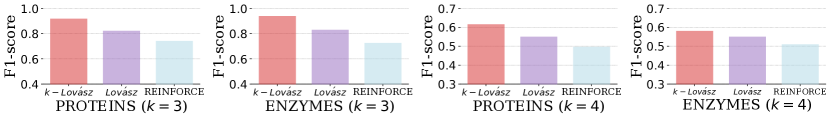
Figure 2: $k$-clique constraint satisfaction: higher F1-score is better. The $k$-bounded cardinality Lovasz extension is better aligned with the task and significantly improves over the Lovász extension.

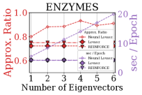
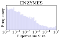
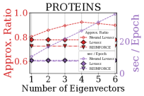
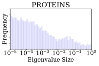
Figure 3: Left: Runtime and performance of neural SFEs on MaxClique using different numbers of eigenvectors. Right: Histogram of spectrum of matrix $\mathbf{X}$, outputted by a GNN trained on MaxClique.

Constraint satisfaction problems ask if there exists a set satisfying a given set of conditions (Kumar, 1992; Cappart et al., 2021b). In this section, we apply SFEs to the $k$-clique problem: given a graph, determine if it contains a clique of size $k$ or more. We test on the ENZYMES and PROTEINS datasets. Since satisfiability is a binary classification problem we evaluate using F1 score.

Results. Figure 2 shows that by specifically searching over sets of size $k$ using the cardinality constrained Lovász extension from Section 3.1, we significantly improve performance compared to the Lovász extension, and REINFORCE. This illustrates the value of SFEs in allowing task-dependent considerations (in this case a cardinality constraint) to be built into extension design.

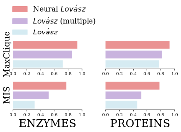
Figure 4: Neural SFEs outperform a naive alternative high-dimensional extension.

5.3 Training Error as a Classification Objective

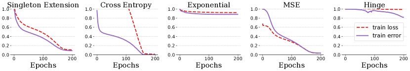
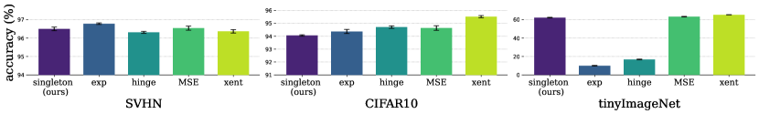
Figure 6: Top: Additional experimental results on the tinyImageNet dataset. Bottom: test accuracies of different losses. The singleton extension performs broadly comparably to other losses.

During training the performance of a classifier $h$ is typically assessed using the training error $\frac{1}{n}\sum_{i=1}^{n}\mathbf{1}\{y_{i}\neq h(x_{i})\}$. Since training error itself is non-differentiable, it is standard to train $h$ to optimize a differentiable surrogate such as the cross-entropy loss. Here we offer an alternative training method by continuously extending the non-differentiable mapping $\hat{y}\mapsto\mathbf{1}\{y_{i}\neq\hat{y}\}$. This map is a set function defined on single item sets, so we use the singleton extension (definition in Section 3.1). Our goal is to demonstrate that the resulting differentiable loss function closely tracks the training error, and can be used to minimize it. We do not focus on test time generalization. Figure 6 shows the results. The singleton extension loss (left plot) closely tracks the true training error at the same numerical scale, unlike other common loss functions (see Appendix G for setup details). While we leave further consideration to future work, training error extensions may be useful for model calibration (Kennedy & O’Hagan, 2001) and uncertainty estimation (Abdar et al., 2021).

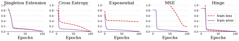
Figure 5: Top: CIFAR10. Bottom: SVHN. The singleton extension loss (left) is the only loss that approximates the true non-differentiable training error at the same numerical scale.

5.4 Ablations

Number of Eigenvectors. Figure 3 compares the runtime and performance of neural SFEs using only the top-$k$ eigenvectors from the eigendecomposition $\mathbf{X}=\sum_{i=1}^{n}\lambda_{i}\mathbf{x}_{i}\mathbf{x}_{i}^{\top}$ with $k\in\{1,2,3,4,5,6\}$ on the maximum clique problem. For both ENZYMES and PROTEINS, performance increases with $k$—easily outperforming scalar SFEs and REINFORCE—until saturation around $k=4$, while runtime grows linearly with $k$. Histograms of the eigenvalues produced by trained networks show a rapid decay in the spectrum, suggesting that the smaller eigenvalues have little effect on $\mathfrak{F}$.

Comparison to Naive High-Dimensional Extension. We compare neural SFEs to a naive high-dimensional alternative which, given an $n\times d$ matrix $\mathbf{X}$ simply computes a scalar SFE on each column independently and sums them up. This naive function design is not an extension, and the dependence on the $d$ dimensions is linearly separable, in contrast to the complex non-linear interactions between columns of $\mathbf{X}$ in neural SFEs. Figure 4 shows that this naive extension, whilst improving over one-dimensional extensions, performs considerably worse than neural SFEs.

6 Related Work

Neural combinatorial optimization Our experimental setup largely follows recent work on unsupervised neural combinatorial optimization (Karalias & Loukas, 2020; Schuetz et al., 2022; Xu et al., 2020; Toenshoff et al., 2021; Amizadeh et al., 2018), where continuous relaxations of discrete objectives are utilized. In that context, it is important to take into account the key conceptual and methodological differences of our approach. For instance, in the unsupervised Erdős goes neural (EGN) framework from Karalias & Loukas (2020), the probabilistic relaxation and the proposed choice of distribution can be viewed as instantiating a multilinear extension. As explained earlier, this extension is costly in the general case (since $f$ must be evaluated $2^{n}$ times, and summed) but can be computed efficiently in closed form in certain cases. On the other hand, our extension framework offers multiple options for efficiently computable extensions without imposing any further conditions on the set function. For example, one could efficiently (linear time in $n$) compute the scalar and neural Lovász extensions of any set function with only black-box access to the function. This renders our framework more broadly applicable. Furthermore, EGN incorporates the problem constraints additively in the loss function. In contrast to that, our extension framework does not require any commitment to a specific formulation in order to obtain a differentiable loss. This provides more flexibility in modelling the problem, as we can combine the cost function and the constraints in various other ways (e.g., multiplicatively). For general background on neural combinatorial optimization, we refer the reader to the surveys (Bengio et al., 2021; Cappart et al., 2021a; Mazyavkina et al., 2021).

Lifting to high-dimensional spaces. Neural SFEs are heavily inspired by the Goemans-Williamson (Goemans & Williamson, 1995) algorithm and other SDP techniques (Iguchi et al., 2015), which lift problems onto higher dimensional spaces, solve them, and then project back down. Our approach to lifting set functions to high dimensions is motivated by the algorithmic alignment principle (Xu et al., 2019): neural networks whose computations emulate classical algorithms often generalize better with improved sample complexity (Yan et al., 2020; Li et al., 2020; Xu et al., 2019). Emulating algorithmic and logical operations is the focus of Neural Algorithmic Reasoning (Veličković et al., 2019; Dudzik & Veličković, 2022; Deac et al., 2021) and work on knowledge graphs (Hamilton et al., 2018; Ren et al., 2019; Arakelyan et al., 2020), which also emphasize operating in higher dimensions.

Extensions. Scalar SFEs use an LP formulation of the convex closure (El Halabi, 2018, Def. 20), a classical approach for defining convex extensions of discrete functions (Murota, 1998, Eq. 3.57). See Bach (2019) for a study of extensions of submodular functions. The constraints of our dual LP arise in contexts from global optimization (Tawarmalani & Sahinidis, 2002) to barycentric approximation and interpolation schemes in computer graphics (Guessab, 2013; Hormann, 2014). Convex extensions have also been used for combinatorial penalties with structured sparsity (Obozinski & Bach, 2012, 2016), and general minimization algorithms for set functions (El Halabi & Jegelka, 2020).

Stochastic gradient estimation. SFEs produce gradients for $f$ requiring only black-box access. There is a wide literature on sampling-based approaches to gradient estimation, for instance the REINFORCE algorithm (Williams, 1992) (i.e., score function estimator). However, sampling introduces noise which can cause unstable training and convergence issues, prompting significant study of variance reducing control variates (Gu et al., 2017; Liu et al., 2018; Grathwohl et al., 2018; Wu et al., 2018; Cheng et al., 2020). SFEs can avoid sampling (and noise) all-together, as our extensions are differentiable and can be computed deterministically. A closely related, yet distinct, task is to produce gradients through sampling operations, which introduce non-differentiable nodes in neural network computation graphs. The Straight-Through Estimator (Bengio et al., 2013), arguably the simplest solution, treats sampling as the identity map in the backward pass, yielding biased gradient estimates. The Gumbel-Softmax trick (Maddison et al., 2017; Jang et al., 2017), provides an alternative method to sample from categorical distributions (also benefiting from variance reduction (Paulus et al., 2020a)). The trick can be seen through the lens of the more general Perturb-and-MAP framework that treats sampling as a perturbed optimization program. This framework has since been used to generalize the trick to more complex distributions (Paulus et al., 2020b) and to differentiate through the parameters of exponential families for learning and combinatorial tasks (Niepert et al., 2021). Broadly, these techniques relax a discrete distribution into a continuous one by utilizing a noise distribution and assuming access to a continuous loss function. SFEs are complementary to this setup, addressing the problem of designing continuous extensions.

Differentiating through convex programs and algorithms. Recent years have seen a surge of interest in combining neural networks with solvers (e.g., LP solvers) and/or algorithms in differentiable end to end pipelines (Agrawal et al., 2019; Amos & Kolter, 2017; Paulus et al., 2021; Pogančić et al., 2019; Wang et al., 2019). Whilst sharing the algorithmic alignment motivation of SFEs, the convex programming connection is mostly cosmetic: these works directly embed solvers into network architectures, while SFEs use convex programs as an analytical tool, without requiring solver access.

7 Conclusion

We introduced Neural Set Function Extensions, a framework that enables evaluating set functions on continuous and high dimensional representations. We showed how to construct such extensions and demonstrated their viability in a range of tasks including combinatorial optimization and image classification. Notably, neural extensions deliver good results and improve over their scalar counterparts, further affirming the benefits of problem-solving in high dimensions.

8 Acknowledgements

NK would like to thank Marwa El Halabi, Mario Sanchez, Mehmet Fatih Sahin, and Volkan Cevher for the feedback and fruitful discussions. NK and AL would like to thank the Swiss National Science Foundation for supporting this work in the context of the project “Deep Learning for Graph-Structured Data” (grant number PZ00P2179981). SJ and JR acknowledge support from NSF CAREER award 1553284, NSF award 1717610, and the NSF AI Institute TILOS.

Checklist

1. For all authors…

   1. Do the main claims made in the abstract and introduction accurately reflect the paper’s contributions and scope? [Yes] All claims made are backed. up either empirically or theoretically.

   2. Did you describe the limitations of your work? [Yes] See Appendix I.1.

   3. Did you discuss any potential negative societal impacts of your work? [Yes] See Appendix I.2.

   4. Have you read the ethics review guidelines and ensured that your paper conforms to them? [Yes] We have read the guidelines, and confirmed that our paper conforms.

2. If you are including theoretical results…

   1. Did you state the full set of assumptions of all theoretical results? [Yes] All theoretical result are stated exactly.

   2. Did you include complete proofs of all theoretical results? [Yes] See Appendix for proofs.

3. If you ran experiments…

   1. Did you include the code, data, and instructions needed to reproduce the main experimental results (either in the supplemental material or as a URL)? [Yes] See anonymized URL for all code.

   2. Did you specify all the training details (e.g., data splits, hyperparameters, how they were chosen)? [Yes] See Appendix F and Appendix G

   3. Did you report error bars (e.g., with respect to the random seed after running experiments multiple times)? [Yes] Except in cases where HPO was run. In these cases we report the test performance of the. model with best validation performance.

   4. Did you include the total amount of compute and the type of resources used (e.g., type of GPUs, internal cluster, or cloud provider)? [Yes] See Appendix E.

4. If you are using existing assets (e.g., code, data, models) or curating/releasing new assets…

   1. If your work uses existing assets, did you cite the creators? [Yes] We cite all creators of. existing assets, either in the main paper or appendix.

   2. Did you mention the license of the assets? [Yes] Yes, see Appendix E.

   3. Did you include any new assets either in the supplemental material or as a URL? [Yes] We provide anonymized code. Open source code will be released after review.

   4. Did you discuss whether and how consent was obtained from people whose data you’re using/curating? [Yes] See Appendix E.

   5. Did you discuss whether the data you are using/curating contains personally identifiable information or offensive content? [Yes] See Appendix E.

5. If you used crowdsourcing or conducted research with human subjects…

   1. Did you include the full text of instructions given to participants and screenshots, if applicable? [N/A] No crowdsourcing or human subjects used.

   2. Did you describe any potential participant risks, with links to Institutional Review Board (IRB) approvals, if applicable? [N/A] No crowdsourcing or human subjects used.

   3. Did you include the estimated hourly wage paid to participants and the total amount spent on participant compensation? [N/A] No crowdsourcing or human subjects used.

Appendix A Optimization programs: extended discussion

In this section, we provide an extended discussion of the key components of our LP and SDP formulations and the relationships between them. Apart from supplying derivations, another goal of this section is to illustrate that there is in fact flexibility in the exact choice of formulation for the LP (and consequently the SDP). We provide details on possible variations as part of this discussion as a guide to users who may wish to adapt the SFE framework.

A.1 LP formulation: Derivation of the dual.

First, recall that our primal LP is defined as

$$\underset{\mathbf{z},b\in\mathbb{R}^{n}\times\mathbb{R}}{\max}\{\mathbf{x}^{\top}\mathbf{z}+b\}\ \text{ subject to }\ \mathbf{1}_{S}^{\top}\mathbf{z}+b\leq f(S)\ \text{ for all }S\subseteq[n].$$

The dual is

$$\underset{\{y_{S}\geq 0\}_{S\subseteq[n]}}{\min}\sum_{S\subseteq[n]}y_{S}f(S)\text{ subject to }\sum_{S\subseteq[n]}y_{S}\mathbf{1}_{S}=\mathbf{x},\ \sum_{S\subseteq[n]}y_{S}=1,\ \text{ for all }S\subseteq[n].$$

In order to standardize the derivation, we first convert the primal maximization problem into minimization (this will be undone at the end of the derivation). We have

$$\underset{\mathbf{z},b\in\mathbb{R}^{n}\times\mathbb{R}}{\min}\{-\mathbf{x}^{\top}\mathbf{z}-b\}\text{ subject to }\ \mathbf{1}_{S}^{\top}\mathbf{z}+b\leq f(S)\ \text{ for all }S\subseteq[n].$$ (3)

The Lagrangian is

$$\underset{y_{S}\geq 0}{\mathcal{L}(\mathbf{z},y_{S},b)} =-\mathbf{x}^{\top}\mathbf{z}-b-\sum_{S\subseteq[n]}y_{S}(f(S)-\mathbf{1}_{S}^{\top}\mathbf{z}-b)$$ (4)

$$=-\sum_{S\subseteq[n]}y_{S}f(S)+(\sum_{S\subseteq[n]}y_{S}\mathbf{1}_{S}^{\top}-\mathbf{x}^{\top})\mathbf{z}+b(\sum_{S\subseteq[n]}y_{S}-1)$$ (5)

The optimal solution $\mathbf{p}^{*}$ to the primal problem is then

$$\mathbf{p}^{*} =\underset{\mathbf{z},b}{\min{}}\underset{y_{S}\geq 0}{\max{}}\mathcal{L}(\mathbf{z},y_{S},b)$$ (6)

$$=\underset{y_{S}\geq 0}{\max{}}\underset{\mathbf{z},b}{\min{}}\mathcal{L}(\mathbf{z},y_{S},b)$$ (strong duality)

$$=\mathbf{d}^{*},$$ (7)

where $\mathbf{d}^{*}$ is the optimal solution to the dual. From the Lagrangian,

$$\underset{\mathbf{z},b}{\min{}}\mathcal{L}(\mathbf{z},y_{S},b)=\begin{cases}-\sum_{S\subseteq[n]}y_{S}f(S),\text{ if }\sum_{S\subseteq[n]}y_{S}\mathbf{1}_{S}=\mathbf{x}\text{ and }\sum_{S\subseteq[n]}y_{S}=1,\\ -\infty,\text{ otherwise}.\end{cases}$$ (8)

Thus, we can write the dual problem as

$$\mathbf{d}^{*}=\underset{y_{S}\geq 0}{\max{}}-\sum_{S\subseteq[n]}y_{S}f(S)\text{ subject to }\sum_{S\subseteq[n]}y_{S}\mathbf{1}_{S}=\mathbf{x}\text{ and }\sum_{S\subseteq[n]}y_{S}=1.$$ (9)

Our proposed dual formulation is then obtained by switching from maximization to minimization and negating the objective. It can also be verified that by taking the dual of our dual, the primal is recovered (see El Halabi (2018, Def. 20) for the derivation).

A.2 Connections to submodularity, related linear programs, and possible alternatives.

Our LP formulation depends on a linear program known to correspond to the convex closure (Murota, 1998, Eq. 3.57) (convex envelope) of a discrete function. Some readers may recognize the formal similarities of this formulation with the one used to define the Lovász extension (Bilmes, 2022). Namely, for $\mathbf{x}\in\mathbb{R}^{n}$ we can define the Lovász Extension as

$$\mathfrak{F}(\mathbf{x})=\underset{\mathbf{z}\in\mathcal{B}_{f}}{\text{max }}\mathbf{x}^{\top}\mathbf{z},$$ (10)

where the feasible set, known as the base polytope of a submodular function, is defined as $\mathcal{B}_{f}=\{\mathbf{z}\in\mathbb{R}^{n}\mathrel{\mathop{\mathchar 58\relax}}\mathbf{z}^{\top}\mathbf{1}_{S}\leq f(S)\;S\subset[n],\text{ and }\mathbf{z}^{\top}\mathbf{1}_{S}=f(S)\text{ when }S=[n]\}$. Base polytopes are also known as generalized permutahedra and have rich connections to the theory of matroids, since matroid polytopes belong to the class of generalized permutahedra Ardila et al. (2010).

An alternative option is to consider $\mathbf{x}\in\mathbb{R}^{n}_{+}$, then the Lovász extension is given by

$$\mathfrak{F}(\mathbf{x})=\underset{\mathbf{z}\in\mathcal{P}_{f}}{\text{max }}\mathbf{x}^{\top}\mathbf{z},$$ (11)

where $\mathcal{P}_{f}$ is the submodular polyhedron as defined in our original primal LP. The subtle differences between those formulations lead to differences in the respective dual formulations. In principle, those formulations can be just as easily used to define set function extensions. Overall, there are three key considerations when defining a suitable LP:

• The constraints of the primal.

• The domain of the primal variables $\mathbf{z},b$ and the cost $\mathbf{x}$.

• The properties of the function being extended.

Below, we describe a few illustrative example cases for different choices of the above:

• Adding the constraint $\mathbf{z}^{\top}\mathbf{1}_{S}=f(S)\text{ when }S=[n]$ leads to $y_{[n]}\in\mathbb{R}^{n}$ for the dual. This implies that the coefficients cannot be interpreted as probabilities in general which is what provides the guarantee that the extension will not introduce any spurious minima. $\sum_{S\subseteq[n]}y_{S}=1$ is just an affine hull constraint in that case.

• For $b=0$, the constraint $\sum_{S\subseteq[n]}y_{S}=1$ is not imposed in the dual and the probabilistic interpretation of the extension cannot be guaranteed. Examples that do not rely on this constraint include the homogeneous convex envelope (El Halabi et al., 2018) and the Lovász extension as presented above. However, even for $b=0$, from the definition of the Lovász extension it is easy to see that it retains the probabilistic interpretation when $\mathbf{x}\in[0,1]$.

• Consider a feasible set defined by $\mathcal{P}_{f}\bigcap\mathbb{R}^{n}_{+}$ and let $\mathbf{x}\in\mathbb{R}^{n}_{+}$. If the function $f$ is submodular, non-decreasing and normalized so that $f(\varnothing)=0$ (e.g., the rank function of a matroid), then the feasible set is called polymatroid and $f$ is a polymatroid function. Again, in that case the Lovász extension achieves the optimal objective value (Schrijver et al., 2003, Eq. 44.32). In that case, the constraint $\sum_{S\subseteq[n]}y_{S}\mathbf{1}_{S}=\mathbf{x}$ of the dual is relaxed to $\sum_{S\subseteq[n]}y_{S}\mathbf{1}_{S}\geq\mathbf{x}$. This feasible set of the dual will allow for more flexible definitions of an extension but it comes at the cost of generality. For instance, for a submodular function that is not non-decreasing, one cannot obtain the Lovász extension as a feasible solution to the primal LP, and the solutions to this LP will not be the convex envelope in general.

A.3 SDP formulation: The geometric intuition of extensions and deriving the dual.

In order to motivate the SDP formulation, first we have to identify the essential ingredients of the LP formulation. First, the constraint $\sum_{S\subseteq[n]}y_{S}\mathbf{1}_{S}=\mathbf{x}$ captures the simple idea that each continuous point is expressed as a combination of discrete ones, each representing a different set, which is at the core of our extensions. Then, ensuring that the continuous point lies in the convex hull of those discrete points confers additional benefits w.r.t. optimization and offers a probabilistic perspective.

Consider the following example. The Lovász extension identifies each continuous point in the hypercube with a simplex. Then the continuous point is viewed as an expectation over a distribution supported on the simplex corners. The value of the set function at a continuous point is then the expected value of the function over those corners under the same distribution, i.e., $\mathbb{E}_{S\sim p_{\mathbf{x}}}[\mathbf{1}_{S}]=\mathbf{x}$ leads to $\mathbb{E}_{S\sim p_{\mathbf{x}}}[f(S)]=\mathfrak{F}(\mathbf{x})$. As long as the distribution $p_{\mathbf{x}}$ can be differentiated w.r.t $\mathbf{x}$, we obtain an extension that can be used with gradient-based optimization. It is clear that the construction depends on being able to identify a small convex set of discrete vectors that can express the continuous one.

This can be formulated in higher dimensions, particularly in the space of PSD matrices. A natural way to represent sets in high dimensions is through rank one matrices that are outer products of the indicator vectors of the sets, i.e., $\mathbf{1}_{S}\mathbf{1}_{S}^{\top}$ is the matrix representation of $S$ similar to how $\mathbf{1}_{S}$ is the vector representation. Hence, in the space of matrices, our goal will be again to identify a set of discrete matrices that represents sets that can express a matrix of continuous values.

The above considerations set the stage for a transition from linear programming to semidefinite programming, where the feasible sets are spectrahedra. Our SDP formulation attempts to capture the intuition described in the previous paragraphs while also maintaining formal connections to the LP by showing that feasible LP regions correspond to feasible SDP regions by simply projecting the LP regions on the space of diagonal matrices (see Proposition 2).

Derivation of the dual.

Recall that our primal SDP is defined as

$$\max_{\mathbf{Z}\succeq 0,b\in\mathbb{R}}\{\text{Tr}(\mathbf{X^{\top}Z})+b\}\text{ subject to }\frac{1}{2}\text{Tr}((\mathbf{1}_{S}\mathbf{1}_{T}^{\top}+\mathbf{1}_{T}\mathbf{1}_{S}^{\top})\mathbf{Z})+b\leq f(S\cap T)\text{ for }S,T\subseteq[n].$$ (12)

We will show that the dual is

$$\min_{\{y_{S,T}\geq 0\}}\sum_{S,\subseteq[n]}y_{S,T}f(S\cap T)\ \text{ subject to }\ \mathbf{X}\preceq\sum_{S,T\subseteq[n]}\frac{1}{2}y_{S,T}(\mathbf{1}_{S}\mathbf{1}_{T}^{\top}+\mathbf{1}_{T}\mathbf{1}_{S}^{\top})\ \ \text{ and }\sum_{S,T\subseteq[n]}y_{{S,T}}=1.$$ (13)

As before, we convert the primal to a minimization problem:

$$\max_{\mathbf{Z}\succeq 0,b\in\mathbb{R}}\{-\text{Tr}(\mathbf{X^{\top}Z})-b\}\text{ subject to }\frac{1}{2}\text{Tr}((\mathbf{1}_{S}\mathbf{1}_{T}^{\top}+\mathbf{1}_{T}\mathbf{1}_{S}^{\top})\mathbf{Z})+b\leq f(S\cap T)\text{ for }S,T\subseteq[n].$$ (14)

First, we will standardize the formulation by converting the inequality constraints into equality constraints. This can be achieved by adding a positive slack variable $d_{S,T}$ to each constraint such that

$$\frac{1}{2}\text{Tr}((\mathbf{1}_{S}\mathbf{1}_{T}^{\top}+\mathbf{1}_{T}\mathbf{1}_{S}^{\top})\mathbf{Z})+b+d_{S,T}=f(S\cap T).$$ (15)

In matrix notation this is done by introducing the positive diagonal slack matrix $\mathbf{D}$ to the decision variable $\mathbf{Z}$, and extending the symmetric matrices in each constraint

$$\mathbf{Z}^{\prime}=\begin{bmatrix}\mathbf{Z}&0\\ 0&\mathbf{D}\end{bmatrix},\quad\mathbf{X}^{\prime}=\begin{bmatrix}\mathbf{X}&0\\ 0&0\end{bmatrix},\quad\mathbf{A}_{S,T}^{\prime}=\begin{bmatrix}\frac{1}{2}(\mathbf{1}_{S}\mathbf{1}_{T}^{\top}+\mathbf{1}_{T}\mathbf{1}_{S}^{\top})&0\\ 0&\text{diag}(\mathbf{e}_{S,T})\end{bmatrix},$$ (16)

where $\text{diag}(\mathbf{e}_{S,T})$ is a diagonal matrix where all diagonal entries are zero except at the diagonal entry corresponding to the constraint on $S,T$ which has a $1$. Using this reformulation, we obtain an equivalent SDP in standard form:

$$\max_{\mathbf{Z^{\prime}}\succeq 0,b\in\mathbb{R}}\{-\text{Tr}(\mathbf{X^{\prime\top}Z^{\prime}})-b\}\text{ subject to }\text{Tr}(\mathbf{A}_{S,T}^{\prime}\mathbf{Z}^{\prime})+b=f(S\cap T)\text{ for }S,T\subseteq[n].$$ (17)

Next, we form the Lagrangian which features a decision variable $y_{S,T}$ for each inequality, and a dual matrix variable $\bm{\Lambda}$. We have

$$\mathcal{L}(\mathbf{Z}^{\prime},b,y_{S,T},\bm{\Lambda}) =-\text{Tr}(\mathbf{X^{\prime\top}Z^{\prime}})-b-\sum_{S,T\subseteq[n]}y_{S,T}\left(2f(S\cap T)-\text{Tr}(\mathbf{A}_{S,T}^{\prime}\mathbf{Z}^{\prime})-b\right)-\text{Tr}(\bm{\Lambda}\mathbf{Z^{\prime}})$$ (18)

$$=\text{Tr}\left(((\sum_{S,T\subseteq[n]}y_{S,T}\mathbf{A}_{S,T}^{\prime})-\mathbf{X^{\prime}}-\bm{\Lambda})\mathbf{Z}^{\prime}\right)+b(\sum_{S,T\subseteq[n]}y_{S,T}-1)-\sum_{S,T\subseteq[n]}y_{S,T}f(S\cap T)$$ (19)

For the solution to the primal $\mathbf{p}^{*}$, we have

$$\mathbf{p}^{*} =\underset{\mathbf{Z}^{\prime},b}{\min}\underset{\bm{\Lambda},y_{S,T}}{\max}\mathcal{L}(\mathbf{Z}^{\prime},b,y_{S,T},\bm{\Lambda})$$ (20)

$$\geq\underset{\bm{\Lambda},y_{S,T}}{\max}\underset{\mathbf{Z}^{\prime},b}{\min{}}\mathcal{L}(\mathbf{Z}^{\prime},b,y_{S,T},\bm{\Lambda})$$ (weak duality)

$$=\mathbf{d}^{*}.$$ (21)

For our Lagrangian we have the dual function

$$\underset{\mathbf{Z^{\prime}},b}{\min{}}\mathcal{L}(\mathbf{Z}^{\prime},b,y_{S,T},\bm{\Lambda})=\begin{cases}0,\text{ if }\bm{\Lambda}\succeq 0,\\ -\infty,\text{ otherwise }.\end{cases}$$ (22)

Thus, the dual function $\underset{\mathbf{Z}^{\prime},b}{\min{}}\mathcal{L}(\mathbf{Z}^{\prime},b,y_{S,T},\bm{\Lambda})$ takes non-infinite values under the conditions

$$(\sum_{S,T\subseteq[n]}y_{S,T}\mathbf{A}_{S,T}^{\prime})-\mathbf{X^{\prime}}-\bm{\Lambda} =0,$$ (23)

$$\bm{\Lambda} \succeq 0,$$ (24)

$$\text{ and }\sum_{S,T\subseteq[n]}y_{S,T}-1 =0.$$ (25)

The first two conditions imply the linear matrix inequality (LMI)

$$\sum_{S,T\subseteq[n]}y_{S,T}\mathbf{A}_{S,T}^{\prime}-\mathbf{X^{\prime}}\succeq 0. \bm{\Lambda}\succeq 0$$ ()

From the definition of $\mathbf{A}_{S,T}^{\prime}$ we know that its additional diagonal entries will correspond to the variables $y_{S,T}$. Combined with the conditions above, we arrive at the constraints of the dual

$$y_{S,T} \geq 0,$$ (26)

$$\sum_{S,T\subseteq[n]}\frac{1}{2}y_{S,T}(\mathbf{1}_{S}\mathbf{1}_{T}^{\top}+\mathbf{1}_{T}\mathbf{1}_{S}^{\top}) \succeq\mathbf{X},$$ (27)

$$\sum_{S,T\subseteq[n]}y_{S,T} =1.$$ (28)

This leads us to the dual formulation

$$\underset{y_{S,T}\geq 0}{\max{}}-\sum_{S,T\subseteq[n]}y_{S,T}f(S\cap T)\text{ subject to }\sum_{S,T\subseteq[n]}\frac{1}{2}y_{S,T}(\mathbf{1}_{S}\mathbf{1}_{T}^{\top}+\mathbf{1}_{T}\mathbf{1}_{S}^{\top}) \succeq\mathbf{X}\text{ and }\sum_{S,T\subseteq[n]}y_{S,T}=1.$$ (29)

Then, we can obtain our original dual by switching to minimization and negating the objective.

Appendix B Scalar Set Function Extensions Have No Bad Minima

In this section we re-state and prove the results from Section 3. The first result concerns the minima of $\mathfrak{F}$, showing that the minimum value is the same as that of $f$, and no additional minima are added (besides convex combinations of discrete minimizers). These properties are especially desirable when using an extension $\mathfrak{F}$ as a loss function (see Section 5) since it is important that $\mathfrak{F}$ drive the neural network $\text{NN}_{1}$ towards producing discrete $\mathbf{1}_{S}$ outputs.

Proposition 4 (Scalar SFEs have no bad minima).

If $\mathfrak{F}$ is a scalar SFE of $f$ then:

1. $\min_{\mathbf{x}\in\mathcal{X}}\mathfrak{F}(\mathbf{x})=\min_{S\subseteq[n]}f(S)$

2. $\operatorname*{arg\,min}_{\mathbf{x}\in\mathcal{X}}\mathfrak{F}(\mathbf{x})\subseteq\text{Hull}\big{(}\operatorname*{arg\,min}_{\mathbf{1}_{S}\mathrel{\mathop{\mathchar 58\relax}}S\subseteq[n]}f(S)\big{)}$

Proof.

The inequality $\min_{\mathbf{x}\in\mathcal{X}}\mathfrak{F}(\mathbf{x})\leq\min_{S\subseteq[n]}f(S)$ automatically holds since $\min_{S\subseteq[n]}f(S)=\min_{\mathbf{1}_{S}\mathrel{\mathop{\mathchar 58\relax}}S\subseteq[n]}\mathfrak{F}(\mathbf{1}_{S})$, and $\{\mathbf{1}_{S}\mathrel{\mathop{\mathchar 58\relax}}S\subseteq[n]\}\subseteq\mathcal{X}$. So it remains to show the reverse. Indeed, letting $\mathbf{x}\in\mathcal{X}$ be an arbitrary point we have,

$$\mathfrak{F}(\mathbf{x}) =\mathbb{E}_{S\sim p_{\mathbf{x}}}[f(S)]$$

$$=\sum_{S\subseteq[n]}p_{\mathbf{x}}(S)\cdot f(S)$$

$$\geq\sum_{S\subseteq[n]}p_{\mathbf{x}}(S)\cdot\min_{S\subseteq[n]}f(S)$$

$$=\min_{S\subseteq[n]}f(S)$$

where the last equality simply uses the fact that $\sum_{S\subseteq[n]}p_{\mathbf{x}}(S)=1$. This proves the first claim.

To prove the second claim, suppose that $\mathbf{x}$ minimizes $\mathfrak{F}(\mathbf{x})$ over $\mathbf{x}\in\mathcal{X}$. This implies that the inequality in the above derivation must be tight, which is true if and only if

$$p_{\mathbf{x}}(S)\cdot f(S)=p_{\mathbf{x}}(S)\cdot\min_{S\subseteq[n]}f(S)\quad\text{ for all }S\subseteq[n].$$

For a given $S$, this implies that either $p_{\mathbf{x}}(S)=0$ or $f(S)=\min_{S\subseteq[n]}f(S)$. Since $\mathbf{x}=\mathbb{E}_{p_{\mathbf{x}}}[{\bm{1}}_{S}]=\sum_{S\subseteq[n]}p_{\mathbf{x}}(S)\cdot{\bm{1}}_{S}=\sum_{S\mathrel{\mathop{\mathchar 58\relax}}p_{\mathbf{x}}(S)>0}p_{\mathbf{x}}(S)\cdot{\bm{1}}_{S}$. This is precisely a convex combination of points ${\bm{1}}_{S}$ for which $f(S)=\min_{S\subseteq[n]}f(S)$. Since $\mathfrak{F}$ is a convex combination of exactly this set of points ${\bm{1}}_{S}$, we have the second claim.

∎

Appendix C Examples of Vector Set Function Extensions

This section re-defines the vector SFEs given in Section 3.1, and prove that they satisfy the definition of an SFEs. One of the conditions we must check is that $\mathfrak{F}$ is continuous. A sufficient condition for continuity (and almost everywhere differentiability) that we shall use for a number of constructions is to show that $\mathfrak{F}$ is Lipschitz. A very simple computation shows that it suffices to show that $\mathbf{x}\in\mathcal{X}\mapsto p_{\mathbf{x}}(S)$ is Lipschitz continuous.

Lemma 1.

If the mapping $\mathbf{x}\in[0,1]^{n}\mapsto p_{\mathbf{x}}(S)$ is Lipschitz continuous and $f(S)$ is finite for all $S$ in the support of $p_{\mathbf{x}}$, then $\mathfrak{F}$ is also Lipschitz continuous. In particular, $\mathfrak{F}$ is continuous and almost everywhere differentiable.

Proof.

The Lipschitz continuity of $\mathfrak{F}(\mathbf{x})$ follows directly from definition:

$$\big{|}\mathfrak{F}(\mathbf{x})-\mathfrak{F}(\mathbf{x}^{\prime})\big{|} =\bigg{|}\sum_{S\subseteq[n]}p_{\mathbf{x}}(S)\cdot f(S)-\sum_{S\subseteq[n]}p_{\mathbf{x}^{\prime}}(S)\cdot f(S)\bigg{|}$$

$$=\bigg{|}\sum_{S\subseteq[n]}\big{(}p_{\mathbf{x}}(S)-p_{\mathbf{x}^{\prime}}(S)\big{)}\cdot f(S)\bigg{|}\leq\left(2kL\max_{S\subseteq[n]}f(S)\right)\,\cdot\|\mathbf{x}-\mathbf{x}^{\prime}\|,$$

where $L$ is the maximum Lipschitz constant of $\mathbf{x}\mapsto p_{\mathbf{x}}(S)$ over any $S$ in the support of $p_{\mathbf{x}}$, and $k$ is the maximal cardinality of the support of any $p_{\mathbf{x}}$. ∎

In general $k$ can be trivially bounded by $2^{n}$, so $\mathfrak{F}$ is always Lipschitz. However in may cases the cardinality of the support of any $p_{\mathbf{x}}$ is much smaller than $2^{n}$, leading too a smaller Lipschitz constant. For instance, $k=n$ in the case of the Lovász extension.

C.1 Lovász extension.

Recall the definition: $\mathbf{x}$ is sorted so that $x_{1}\geq x_{2}\geq\ldots\geq x_{d}$. Then the Lovász extension corresponds to taking $S_{i}=\{1,\ldots,i\}$, and letting $p_{\mathbf{x}}({S_{i}})=x_{i}-x_{i+1}$, the non-negative increments of $\mathbf{x}$ (where recall we take $x_{n+1}=0$). All other sets have zero probability. For convenience, we introduce the shorthand notation $a_{i}=p_{\mathbf{x}}(S_{i})=x_{i}-x_{i+1}$

Feasibility.

Clearly all $a_{i}=x_{i}-x_{i+1}\geq 0$, and $\sum_{i=1}^{n}a_{i}=\sum_{i=1}^{n}(x_{i}-x_{i+1})=x_{1}\leq 1$. Any remaining probability mass is assigned to the empty set: $p_{\mathbf{x}}(\varnothing)=1-x_{1}$, which contributes nothing to the extension $\mathfrak{F}$ since $f(\varnothing)=0$ by assumption. All that remains is to check that

$$\sum_{i=1}^{n}p_{\mathbf{x}}(S_{i})\cdot{\bm{1}}_{S_{i}}=\mathbf{x}.$$

For a given $k\in[n]$, note that the only sets $S_{i}$ with non-zero $k$th coordinate are $S_{1},\ldots,S_{k}$, and in all cases $({\bm{1}}_{S_{i}})_{k}=1$. So the $k$th coordinate is precisely $\sum_{i=1}^{k}p_{\mathbf{x}}(S_{i})=\sum_{i=1}^{k}(x_{i}-x_{i+1})=x_{k}$, yielding the desired formula.

Extension.

Consider an arbitrary $S\subseteq[n]$. Since we assume $\mathbf{x}={\bm{1}}_{S}$ is sorted, it has the form ${\bm{1}}_{S}=(\underbrace{1,1,\ldots,1}_{k\text{ times}},0,0,\ldots 0)^{\top}$. Therefore, for each $j<k$ we have $a_{j}=x_{j}-x_{j+1}=1-1=0$ and for each $j>k$ we have $a_{j}=x_{j}-x_{j+1}=0-0=0$. The only non-zero probability is $a_{k}=x_{k}-x_{k+1}=1-0=1$. So,

$$\mathfrak{F}({\bm{1}}_{S})=\sum_{i=1}^{n}a_{i}f(S_{i})=\sum_{i\mathrel{\mathop{\mathchar 58\relax}}i\neq k}a_{i}f(S_{i})+a_{k}f(S_{k})=0+1\cdot f(S_{k})=f(S)$$

where the the final equality follows since by definition $S_{k}$ corresponds exactly to the vector $(\underbrace{1,1,\ldots,1}_{k\text{ times}},0,0,\ldots 0)^{\top}={\bm{1}}_{S}$ and so $S_{k}=S$.

Continuity.

The Lovász is a well-known extension, whose properties have been carefully studied. In particular it is well known to be a Lipschitz function Bach (2019). However, for completeness we provide a simple proof here nonetheless.

Lemma 2.

Let $p_{\mathbf{x}}$ be as defined for the Lovász extension. Then $\mathbf{x}\mapsto p_{\mathbf{x}}(S)$ is Lipschitz for all $S\subseteq[n]$.

Proof.

First note that $p_{\mathbf{x}}$ is piecewise linear, with one piece per possible ordering $x_{1}\geq x_{2}\geq\ldots\geq x_{n}$ (so $n!$ pieces in total). Within the interior of each piece $p_{\mathbf{x}}$ is linear, and therefore Lipschitz. So in order to prove global Lipschitzness, it suffices to show that $p_{\mathbf{x}}$ is continuous at the boundaries between pieces (the Lipschitz constant is then the maximum of the Lipschitz constants for each linear piece).

Now consider a point $\mathbf{x}$ with $x_{1}\geq\ldots\geq x_{i}=x_{i+1}\geq\ldots\geq x_{n}$. Consider the perturbed point $\mathbf{x}_{\delta}=\mathbf{x}-\delta\mathbf{e}_{i}$ with $\delta>0$, and $\mathbf{e}_{i}$ denoting the $i$th standard basis vector. To prove continuity of $p_{\mathbf{x}}$ it suffices to show that for any $S\in\Omega$ we have $p_{\mathbf{x}_{\delta}}(S)\rightarrow p_{\mathbf{x}}(S)$ as $\delta\rightarrow 0^{+}$.

There are two sets in the support of $p_{\mathbf{x}}$ whose probabilities are different under $p_{\mathbf{x}_{\delta}}$, namely: $S_{i}=\{1,\ldots,i\}$ and $S_{i+1}=\{1,\ldots,i,i+1\}$. Similarly, there are two sets in the support of $p_{\mathbf{x}_{\delta}}$ whose probabilities are different under $p_{\mathbf{x}}$, namely: $S^{\prime}_{i}=\{1,\ldots,i-1,i+1\}$ and $S^{\prime}_{i+1}=\{1,\ldots,i,i+1\}=S_{i+1}$. So it suffices to show the convergence $p_{\mathbf{x}_{\delta}}(S)\rightarrow p_{\mathbf{x}}(S)$ for these four $S$. Consider first $S_{i}$:

$$\big{|}p_{\mathbf{x}_{\delta}}(S_{i})-p_{\mathbf{x}}(S_{i})\big{|}=\big{|}0-(x_{i}-x_{i+1})\big{|}=0$$

where the final equality uses the fact that $x_{i}=x_{i+1}$. Next consider $S_{i+1}=S^{\prime}_{i+1}$:

$$\big{|}p_{\mathbf{x}_{\delta}}(S_{i+1})-p_{\mathbf{x}}(S_{i+1})\big{|}=\big{|}(x^{\prime}_{i+1}-x^{\prime}_{i+2})-(x_{i+1}-x_{i+2})\big{|}=\big{|}(x^{\prime}_{i+1}-x_{i+1})-(x^{\prime}_{i+2}-x_{i+2})\big{|}=0$$

Finally, we consider $S^{\prime}_{i}$:

$$\big{|}p_{\mathbf{x}_{\delta}}(S^{\prime}_{i})-p_{\mathbf{x}}(S^{\prime}_{i})\big{|} =\big{|}(x^{\prime}_{i}-x^{\prime}_{i+1})-(x_{i}-x_{i+1})\big{|}$$

$$=\big{|}(x^{\prime}_{i+1}-x_{i+1})-(x^{\prime}_{i+1}-x_{i+1})\big{|}$$

$$=\big{|}(x_{i+1}-\delta-x_{i+1})-(x^{\prime}_{i+1}-x_{i+1})\big{|}$$

$$=\delta\rightarrow 0$$

completing the proof. ∎

C.2 Bounded cardinality Lovaśz extension.

The bounded cardinality extension coefficients $p_{\mathbf{x}}(S)$ are the coordinates of the vector $\mathbf{y}$, where $\mathbf{y}=\mathbf{S}^{-1}\mathbf{x}$ and the entries $(i,j)$ of the inverse are

$$\mathbf{S}^{-1}(i,j)=\begin{cases}1,\text{ if }(j-i)\text{ mod }k=0\text{ and }i\leq j,\\ -1,\text{ if }(j-i)\text{ mod }k=1\text{ and }i\leq j,\\ 0,\text{ otherwise}.\end{cases}$$ (30)

Equivalence to the Lovaśz extension.

We want to show that the bounded cardinality extension is equivalent to the Lovaśz extension when $k=n$. Let $T_{i,k}=\{j\;|\;(j-i)\text{ mod }k=0,\text{ for }i\leq j\leq n,\;j\in\mathbb{Z}_{+}\}$, i.e., $T_{i,k}$ stores the indices where $j-i$ is perfectly divided by $k$. From the analytic form of the inverse, observe that the $i$-th coordinate of $\mathbf{y}$ is $p_{\mathbf{x}}(S_{i})=\sum_{j\in T_{i,k}}(x_{j}-x_{j+1})$. For $k=n$, we have $T_{i,n}=\{j\;|\;(j-i)\text{ mod }n=0\}=\{i\}$, and therefore $p_{\mathbf{x}}(S_{i})=x_{i}-x_{i+1}$, which are the coefficients of the Lovász extension.

Feasibility.

The equation $\mathbf{y}=\mathbf{S}^{-1}\mathbf{x}$ guarantees that the constraint $\mathbf{x}=\sum_{i=1}^{n}y_{S_{i}}\mathbf{1}_{S_{i}}$ is obeyed. Recall that $\mathbf{x}$ is sorted in descending order like in the case of the Lovász extension. Then, it is easy to see that $p_{\mathbf{x}}(S_{i})=\sum_{j\in T_{i,k}}(x_{j}-x_{j+1})\leq x_{i}$, because $x_{i}-x_{i+1}$ is always contained in the summation for $p_{\mathbf{x}}(S_{i})$. Therefore, by restricting $\mathbf{x}$ in the probability simplex it is easy to see that $\sum_{i=1}^{n}p_{\mathbf{x}}(S_{i})\leq\sum_{i=1}^{n}x_{i}=1$. To secure tight equality, we allocate the rest of the mass to the empty set, i.e., $p_{\mathbf{x}}(\varnothing)=1-\sum_{i=1}^{n}p_{\mathbf{x}}(S_{i})$, which does not affect the value of the extension sicne the corresponding Boolean is the zero vector.

Extension.

To prove the extension property we need to show that $\mathfrak{F}(\mathbf{1}_{S})=f(S)$ for all $S$ with $|S|\leq k$. Consider any such set $S$ and recall that we have sorted $\mathbf{1}_{S}$ with arbitrary tie breaks, such that $x_{i}=1$ for $i\leq|S|$ and $x_{i}=0$ otherwise. Due to the equivalence with the Lovaśz extension, the extension property is guaranteed when $k=n$ for all possible sets. For $k<n$, consider the following three cases for $T_{i,k}$.

• When $i>|S|$, $T_{i,k}=\varnothing$ because for sorted $\mathbf{x}$ of cardinality at most $k$, we know for the coordinates that $x_{i}=x_{i+1}=0$. For $i>k$, this implies that $p_{\mathbf{x}}(S_{i})=0$.

• When $i<|S|$, $\sum_{j\in T_{i,k}}(x_{j}-x_{j+1})=0$ because $x_{j}=x_{j+1}=1$ and we have again $p_{\mathbf{x}}(S_{i})=0$.

• When $i=|S|$, observe that $\sum_{j\in T_{i,k}}(x_{j}-x_{j+1})=x_{i}-x_{i+1}=x_{i}$. Therefore, $p_{\mathbf{x}}(S_{i})=1.$ in that case.

Bringing it all together, $\mathfrak{F}(\mathbf{1}_{S})=\sum_{i=1}^{n}p_{\mathbf{x}}f(S_{i})=p_{\mathbf{x}}(S)f(S)=f(S)$ since the sum contains only one nonzero term, the one that corresponds to $i=|S|$.

Continuity.

Similar to the Lovaśz extension, $p_{\mathbf{x}}$ in the bounded cardinality extension is piecewise linear and therefore a.e. differentiable with respect to $\mathbf{x}$, where each piece corresponds to an ordering of the coordinates of $\mathbf{x}$. On the other hand, unlike the Lovaśz extension, the mapping $\mathbf{x}\mapsto p_{\mathbf{x}}(S)$ is not necessarily globally Lipschitz when $k<n$, because it is not guaranteed to be Lipschitz continuous at the boundaries.

C.3 Singleton extension.

Feasibility.

The singleton extension is not dual LP feasible. However, one of the key reasons why feasibility is important is that it implies Proposition 1, which show that optimizing $\mathfrak{F}$ is a reasonable surrogate to $f$. In the case of the singleton extension, however, Proposition 1 still holds even without feasibility for $f$. This includes the case of the training accuracy loss, which can be viewed as minimizing the set function $f(\{\hat{y}\})=-\mathbf{1}\{y_{i}=\hat{y}\}$.

Here we give an alternative proof of Proposition 1 for the singleton extension. Consider the same assumptions as Proposition 1 with the additional requirement that $\min_{S}f(S)<0$ (this merely asserts hat $S=\varnothing$ is not a trivial solution to the minimization problem, and that the minimizer of $f$ is unique. This is true, for example, for the training accuracy objective we consider in Section 5.

Proof of Proposition 1 for singleton extension.

For $\mathbf{x}\in\mathcal{X}=[0,1]^{n}$,

$$\mathfrak{F}(\mathbf{x}) =\sum_{i=1}^{n}p_{\mathbf{x}}(S_{i})f(S_{i})$$

$$=\sum_{i=1}^{n}(x_{i}-x_{i+1})f(S_{i})$$

$$\geq\sum_{i=1}^{n}(x_{i}-x_{i+1})\min_{j\in[n]}f(S_{j})$$

$$\geq(x_{1}-x_{n+1})\min_{j\in[n]}f(S_{j})$$

$$\geq x_{1}\cdot\min_{j\in[n]}f(S_{j})$$

$$\geq\min_{j\in[n]}f(S_{j})$$

where the final inequality follows since $\min_{j\in[n]}f(S_{j})<0$. Taking $\mathbf{x}=(1,0,0,\ldots,0)^{\top}$ shows that all the inequalities can be made tight, and the first statement of Proposition 1 holds. For the second statement, suppose that $\mathbf{x}\in\mathcal{X}=[0,1]^{n}$ minimizes $\mathfrak{F}$. Then all the inequality in the preceding argument must be tight. In particular, tightness of the final inequality implies that $x_{1}=1$. Meanwhile, tightness of the first inequaliity implies that $x_{i}-x_{i+1}=0$ for all $i$ for which $f(S_{i})\neq\min_{j\in[n]}f(S_{j})$, and tightness of the second inequality implies that $x_{n+1}=0$. These together imply that $\mathbf{x}=\mathbf{1}\oplus\mathbf{0}_{n-1}$ where $\mathbf{1}$ is a $1\times 1$ vector with entry equal to one, and $\mathbf{0}_{n-1}$ is an all zeros vectors of length $n-1$, and $\oplus$ denotes concatenation. Since $f(S_{1})=\min_{j\in[n]}f(S_{j})$ is the unique minimize we have that $\mathbf{x}=\mathbf{1}_{S_{1}}\in\text{Hull}\big{(}\operatorname*{arg\,min}_{\mathbf{1}_{S_{i}}\mathrel{\mathop{\mathchar 58\relax}}i\in[n]}f(S_{i})\big{)}$, completing the proof. ∎

Extension.

Consider an arbitrary $i\in[n]$. Since we assume $\mathbf{x}={\bm{1}}_{\{i\}}$ is sorted, we are without loss of generality considering ${\bm{1}}_{\{1\}}=(1,0,\ldots,0,0,\ldots 0)^{\top}$. Therefore, we have $p_{\mathbf{x}}(S_{1})=x_{1}-x_{2}=1-0=1$ and for each $j>1$ we have $p_{\mathbf{x}}(S_{j})=x_{j}-x_{j+1}=0-0=0$. The only non-zero probability is $p_{\mathbf{x}}(S_{1})$, and so

$$\mathfrak{F}({\bm{1}}_{\{1\}})=\sum_{j=1}^{n}p_{\mathbf{x}}(S_{j})f(S_{j})=f(S_{1})=f(\{1\}).$$

Continuity.

The proof of continuity of the singleton extension is a simple adaptation of the proof used for the Lovaśz extension, which we omit.

C.4 Permutations and Involutory Extension.

Feasibility.

It is known that every elementary permutation matrix is involutory, i.e., $\mathbf{SS=I}$. Given such an elementary permutation matrix $\mathbf{S}$, since $\mathbf{S(S}\mathbf{x})=\mathbf{S}p_{\mathbf{x}}=\mathbf{x}$, the constraint $\sum_{S\subseteq[n]}y_{S}\mathbf{1}_{S}=\mathbf{x}$ is satisfied. Furthermore, $\sum_{S\subseteq[n]}y_{S}=1$ can be secured if $\mathbf{x}$ is in the simplex, since the sum of the elements of a vector is invariant to permutations of the entries.

Extension.

If the permutation has a fixed point at the maximum element of $\mathbf{x}$, i.e., it maps the maximum element to itself, then any elementary permutation matrix with such a fixed point yields an extension on singleton vectors. Without loss of generality, let $\mathbf{x}=\mathbf{e}_{1}$, where $\mathbf{e}_{1}$ is the standard basis vector in $\mathbb{R}^{n}$. Then $\mathbf{Se}_{1}=\mathbf{e}_{1}$ and therefore $p_{\mathbf{x}}(\mathbf{e}_{1})=1$. This in turn implies $\mathfrak{F}(\mathbf{e}_{1})=1\cdot f(\mathbf{e}_{1})$. This argument can be easily applied to all singleton vectors.

Continuity.

The permutation matrix $\mathbf{S}$ can be chosen in advance for each $\mathbf{x}$ in the simplex. Since $p_{\mathbf{x}}=\mathbf{S}\mathbf{x}$, the probabilities are piecewise-linear and each piece is determined by the fixed point induced by the maximum element of $\mathbf{x}$. Consequently, $p_{\mathbf{x}}$ depends continuously on $\mathbf{x}$.

C.5 Multilinear extension.

Recall that the multiliniear extension is defined via $p_{\mathbf{x}}(S)=\prod_{i\in S}x_{i}\prod_{i\notin S}(1-x_{i})$ supported on all subsets $S\subseteq[n]$ in general.

Feasibility.

The definition of $p_{\mathbf{x}}(S)$ is equivalent to:

$$p_{\mathbf{x}}(S)=\prod_{i=1}^{n}x_{i}^{y_{i}}(1-x_{i})^{1-y_{i}}$$

where $y_{i}=1$ if $i\in S$ and zero otherwise. That is, $p_{\mathbf{x}}(S)$ is the product of $n$ independent Bernoulli distributions. So we clearly have $p_{\mathbf{x}}(S)\geq 0$ and $\sum_{S\subseteq[n]}p_{\mathbf{x}}(S)=1$. The final feasibility condition, that $\sum_{S\subseteq[n]}p_{\mathbf{x}}(S)\cdot{\bm{1}}_{S}=\mathbf{x}$ can be checked by induction on $n$. For $n=1$ there are only two sets: $\{1\}$ and the empty set. And clearly $p_{\mathbf{x}}(\{1\})\cdot{\bm{1}}_{\{1\}}=x_{1}(1-x_{1})^{0}=x_{1}$, so we have the base case.

Extension.

For any $S\subseteq[n]$ we have $p_{{\bm{1}}_{S}}(S)=\prod_{i\in S}x_{i}\prod_{i\notin S}(1-x_{i})=\prod_{i\in S}1\prod_{i\notin S}(1-0)=1$. So $\mathfrak{F}({\bm{1}}_{S})=\mathbb{E}_{T\sim p_{\mathbf{x}}}f(T)=f(S)$.

Continuity.

Fix and $S\subseteq[n]$. Again we check Lipschitzness. We use $\partial_{x_{k}}$ to denote the derivative operator with respect to $x_{k}$. If $k\in S$ we have

$$\mathinner{\!\left\lvert\partial_{x_{k}}p_{{\bm{1}}_{S}}(S)\right\rvert}=\mathinner{\!\left\lvert\partial_{x_{k}}\prod_{i\in S}x_{i}\prod_{i\notin S}(1-x_{i})\right\rvert}=\prod_{i\in S\setminus\{k\}}x_{i}\prod_{i\notin S}(1-x_{i})\leq 1.$$

Similarly, if $k\notin S$ we have,

$$\mathinner{\!\left\lvert\partial_{x_{k}}p_{{\bm{1}}_{S}}(S)\right\rvert}=\mathinner{\!\left\lvert\partial_{x_{k}}\prod_{i\in S}x_{i}\prod_{i\notin S}(1-x_{i})\right\rvert}=\mathinner{\!\left\lvert-\prod_{i\in S}x_{i}\prod_{i\notin S\cup\{k\}}(1-x_{i})\right\rvert}\leq 1.$$

Hence the spectral norm of the Jacobian $Jp_{\mathbf{x}}(S)$ is bounded, and so $\mathbf{x}\mapsto p_{\mathbf{x}}(S)$ is a Lipschitz map.

Appendix D Neural Set Function Extensions

This section re-states and proves the results from Section 4. To start, recall the definition of the primal LP:

$$\underset{\mathbf{z},b}{\max}\{\mathbf{x}^{\top}\mathbf{z}+b\},\ \text{ where }\ (\mathbf{z},b)\in\mathbb{R}^{n}\times\mathbb{R}\text{ and }\mathbf{1}_{S}^{\top}\mathbf{z}+b\leq f(S)\ \text{ for all }S\subseteq[n].$$

and primal SDP:

$$\max_{\mathbf{Z}\succeq 0,b\in\mathbb{R}}\{\text{Tr}(\mathbf{X^{\top}Z})+b\}\text{ subject to }\frac{1}{2}\text{Tr}((\mathbf{1}_{S}\mathbf{1}_{T}^{\top}+\mathbf{1}_{T}\mathbf{1}_{S}^{\top})\mathbf{Z})+b\leq f(S\cap T)\text{ for }S,T\subseteq[n].$$ (31)

Proposition.

(Containment of LP in SDP) For any $\mathbf{x}\in[0,1]^{n}$, define $\mathbf{X}=\sqrt{\mathbf{x}}\sqrt{\mathbf{x}}^{\top}$ with the square-root taken entry-wise. Then, for any $(\mathbf{z},b)\in\mathbb{R}^{n}_{+}\times\mathbb{R}$ that is primal LP feasible, the pair $(\mathbf{Z},b)$ where $\mathbf{Z}=\text{diag}(\mathbf{z})$, is primal SDP feasible and the objective values agree: $\text{Tr}(\mathbf{X^{\top}Z})=\mathbf{z}^{\top}\mathbf{x}$.

Proof.

We start with the feasibility claim. Suppose that $(\mathbf{z},b)\in\mathbb{R}^{n}_{+}\times\mathbb{R}$ is a feasible solution to the primal LP. We must show that $(\mathbf{Z},b)$ is a feasible solution to the primal SDP with $\mathbf{X}=\sqrt{\mathbf{x}}\sqrt{\mathbf{x}}^{\top}$ and where $\mathbf{Z}=\text{diag}(\mathbf{z})$.

Recall the general formula for the trace of a matrix product: $\text{Tr}(\mathbf{AB})=\sum_{i,j}A_{ij}B_{ji}$. With this in mind, and noting that the $(i,j)$ entry of $\mathbf{1}_{S}\mathbf{1}_{T}^{\top}$ is equal to $1$ if $i,j\in S\cap T$, and zero otherwise, we have for any $S,T\subseteq[n]$ that

$$\frac{1}{2}\text{Tr}((\mathbf{1}_{S}\mathbf{1}_{T}^{\top}+\mathbf{1}_{T}\mathbf{1}_{S}^{\top})\mathbf{Z})=\text{Tr}(\mathbf{1}_{S}\mathbf{1}_{T}^{\top}\mathbf{Z})+b =\sum_{i,j=1}^{n}(\mathbf{1}_{S}\mathbf{1}_{T}^{\top})_{ij}\cdot\text{diag}(\mathbf{z})_{ij}+b$$

$$=\sum_{i,j\in S\cap T}(\mathbf{1}_{S}\mathbf{1}_{T}^{\top})_{ij}\cdot\text{diag}(\mathbf{z})_{ij}+b$$

$$=\sum_{i,j\in S\cap T}\text{diag}(\mathbf{z})_{ij}+b$$

$$=\sum_{i\in S\cap T}z_{i}+b$$

$$={\bm{1}}_{S\cap T}^{\top}\mathbf{z}+b$$

$$\leq f(S\cap T)$$

showing SDP feasibility. That the objective values agree is easily seen since:

$$\text{Tr}(\mathbf{ZX})=\sum_{i,j=1}^{n}\text{diag}(\mathbf{z})_{ij}\cdot\sqrt{x_{i}}\sqrt{x_{j}}=\sum_{i=1}^{n}z_{i}\cdot\sqrt{x_{i}}\sqrt{x_{i}}=\mathbf{x}^{\top}\mathbf{z}.$$

∎

Next, we provide a proof for the construction of neural extensions. Recall the statement of the main result.

Proposition.

Let $p_{\mathbf{x}}$ induce a scalar SFE of $f$. For $\mathbf{X}\in\mathbb{S}_{+}^{n}$ with distinct eigenvalues, consider the decomposition $\mathbf{X}=\sum_{i=1}^{n}\lambda_{i}\mathbf{x}_{i}\mathbf{x}_{i}^{\top}$ and fix

$$p_{\mathbf{X}}(S,T)=\sum_{i=1}^{n}\lambda_{i}\,p_{\mathbf{x}_{i}}(S)p_{\mathbf{x}_{i}}(T)\text{ for all }S,T\subseteq[n].$$ (32)

Then, $p_{\mathbf{X}}$ defines a neural SFE $\mathfrak{F}$ at $\mathbf{X}$.

Proof.

We begin by showing through the eigendecomposition of $\mathbf{X}$ that the $\mathfrak{F}$ defined by $p_{\mathbf{X}}(S,T)$ is dual SDP feasible. It is clear that $\sum_{S,T}p_{\mathbf{X}}(S,T)=1$ as long as $\sum_{i=1}^{n}\lambda_{i}=1$, which can be easily enforced by appropriate normalization of $\mathbf{X}$. Recall from the eigendecomposition we have $\mathbf{X}=\sum_{i=1}^{n}\lambda_{i}\mathbf{v}_{i}\mathbf{v}_{i}^{\top}$ where we have fixed each $\mathbf{v}_{i}\in[0,1]^{n}$ through a sigmoid. Using the scalar SFE $p_{\mathbf{x}}$ we may write each $\mathbf{v}_{i}$ as a convex combination $\mathbf{v}_{i}=\sum_{S}p_{\mathbf{v}_{i}}(S)\mathbf{1}_{S}$. For each $i$ we may use this representation to re-express the outer product of $\mathbf{v}_{i}$ with itself:

$$\mathbf{v}_{i}\mathbf{v}_{i}^{\top} =\big{(}\sum_{S}p_{\mathbf{v}_{i}}(S)\mathbf{1}_{S}\big{)}\big{(}\sum_{T}p_{\mathbf{v}_{i}}(T)\mathbf{1}_{T}\big{)}^{\top}$$

$$={\sum_{S}p_{\mathbf{v}_{i}}(S)^{2}\mathbf{1}_{S}\mathbf{1}_{S}^{\top}}+\sum_{S\neq T}p_{\mathbf{v}_{i}}(S)p_{\mathbf{v}_{i}}(T)(\mathbf{1}_{T}\mathbf{1}_{S}^{\top}+\mathbf{1}_{S}\mathbf{1}_{T}^{\top})$$

$$=\sum_{S,T\subseteq[n]}p_{\mathbf{v_{i}}}(S)p_{\mathbf{v_{i}}}(T)(\mathbf{1}_{S}\mathbf{1}_{T}^{\top}+\mathbf{1}_{T}\mathbf{1}_{S}^{\top})$$

Summing over all eigenvectors $\mathbf{v}_{i}$ yields the relation $\mathbf{X}=\sum_{S,T\subseteq[n]}p_{\mathbf{X}}(S,T)(\mathbf{1}_{S}\mathbf{1}_{T}^{\top}+\mathbf{1}_{T}\mathbf{1}_{S}^{\top})$, proving dual SDP feasibility.

Next, consider an input $\mathbf{X}=\mathbf{1}_{S}\mathbf{1}_{S}^{\top}$. In this case, the only eigenvector is $\mathbf{1}_{S}$ with eigenvalue $\lambda=|S|$ since $\mathbf{X}\mathbf{1}_{S}=\mathbf{1}_{S}(\mathbf{1}_{S}^{\top}\mathbf{1}_{S})=\mathbf{1}_{S}|S|$. That is, $p_{\mathbf{X}}(T^{\prime},T)=p_{\mathbf{1}_{S}}(T^{\prime})p_{\mathbf{1}_{S}}(T)$.

For $\mathbf{X}=\mathbf{1}_{S}\mathbf{1}_{S}^{\top}$, $\mathbf{1}_{S}$ is clearly an eigenvector with eigenvalue $\lambda=|S|$ because $\mathbf{X}\mathbf{1}_{S}=\mathbf{1}_{S}(\mathbf{1}_{S}^{\top}\mathbf{1}_{S})=\mathbf{1}_{S}|S|$. So, taking $\mathbf{\bar{1}}_{S}=\mathbf{1}_{S}/\sqrt{|S|}$ to be the normalized eigenvector of $\mathbf{X}$, we have $\mathbf{X}=|S|\mathbf{\bar{1}}_{S}\mathbf{\bar{1}}_{S}^{\top}=|S|\bigg{(}\frac{\mathbf{1}_{S}}{\sqrt{|S|}}\bigg{)}\bigg{(}\frac{\mathbf{1}_{S}}{\sqrt{|S|}}\bigg{)}^{\top}=p_{\mathbf{X}}(S,S)\mathbf{1}_{S}\mathbf{1}_{S}^{\top}$ for $p_{\mathbf{X}}(S,S)=1$. Therefore, the corresponding neural SFE is

$$\mathfrak{F}(\mathbf{1}_{S}\mathbf{1}_{S}^{\top})=p_{\mathbf{X}}(S,S)f(S\cap S)=f(S).$$

All that remains is to show continuity of neural SFEs. Since the scalar SFE $p_{\mathbf{x}}$ is continuous in $\mathbf{x}$ by assumption, all that remains is to show that the map sending $\mathbf{X}$ to its eigenvector with $i$-th largest eigenvalue is continuous. We handle sign flip invariance of eignevectors by assuming a standard choice for eigenvector signs—e.g., by flipping the sign where necessary to ensure that the first non-zero coordinate is greater than zero. The continuity of the mapping $\mathbf{X}\mapsto\mathbf{v}_{i}$ follows directly from Theorem 2 from Yu et al. (2015), which is a variant of the Davis–Kahan theorem. The result shows that the angle between the $i$-th eigenspaces of two matrices $\mathbf{X}$ and $\mathbf{X}^{\prime}$ goes to zero in the limit as $\mathbf{X}\rightarrow\mathbf{X}^{\prime}$. ∎

Appendix E General Experimental Background Information

E.1 Hardware and Software Setup

All training runs were done on a single GPU at a time. Experiments were either run on 1) a server with 8 NVIDIA RTX 2080 Ti GPUs, or 2) 4 NVIDIA RTX 2080 Ti GPUs. All experiments are run using Python, specifically the PyTorch (Paszke et al., 2019) framework (see licence here). For GNN specific functionality, such as graph data batching, use the PyTorch Geometric (PyG) (Fey & Lenssen, 2019) (MIT License).

We shall open source our code with MIT License, and have provided anonymized code as part of the supplementary material for reviewers.

E.2 Data Details

This paper uses five graph datasets: ENZYMES, PROTEINS, IMDB-BINART, MUTAG, and COLLAB. All data is accessed via the standardized PyG API. In the case of COLLAB, which has 5000 samples available, we subsample the first 1000 graphs only for training efficiency. All experiments Use a train/val/test split ratio of 60/30/10, which is done in exactly one consistent way across all experiments for each dataset.

Appendix F Unsupervised Neural Combinatorial Optimization Experiments

All methods use the same GNN backbone: a combination of GAT Veličković et al. (2018) and Gated Graph Convolution layer (Yujia et al., 2016). We use the Adam optimizer Kingma & Ba (2014) with initial $lr=10^{-4}$ and default PyTorch settings for other parameters Paszke et al. (2019). We use grid search HPO over batch size $\{4,32,64\}$, number of GNN layers $\{6,10,16\}$ network width $\{64,128,256\}$. All models are trained for $200$ epochs. For the model with the best validation performance, we report the test performance and the standard deviation of performance over test graphs as a measure of method reliability.

F.1 Discrete Objectives

Maximum Clique.

For the maximum clique problem, we could simply take $f$ to compute the clique size (with the size being zero if $S$ is not a clique). However, we found that this objective led to poor results and unstable training dynamics. So, instead, we select a discrete objective that yielded the much more stable results across datasets. It is defined for a graph $G=([n],E)$ as,

$$f_{\text{MaxClique}}(S;G)=w(S)q^{c}(S),$$ (33)

where $w$ is a measure of size of $S$ and $q$ measures the density of edges within $S$ (i.e., distance from being a clique). The scalar $c$ is a constant, taken to be $c=2$ in all cases except REINFORCE for which $c=2$ proved ineffective, so we use $c=4$ instead. Specifically, $w(S)=\sum_{i,j\in S}\mathbf{1}\{(i,j)\in E\}$ simply counts up all the edges between nodes in $S$, and $q(S)=-2w(S)/(|S|^{2}-|S|)$ is the ratio (with a sign flip) between the number of edges in $S$, and the number of undirected edges $(|S|^{2}-|S|)/2$ there would be in a clique of size $|S|$. If $G$ were directed, simply remove the factor of $2$. Note that this $f$ is minimized when $S$ is a maximum clique.

Maximum Independent Set.

Similarly for maximum independent set we use the discrete objective,

$$f_{\text{MIS}}(S;G)=w(S)q^{c}(S),$$ (34)

where $w$ is a measure of size of $S$ and $q$ measures the number of edges between nodes in $S$ (the number should be zero for an independent set), and $c=2$ as before. Specifically, we take $w(S)=|S|/n$, and $q(s)=2\sum_{i,j\in S}\mathbf{1}\{(i,j)\in E\}/(|S|^{2}-|S|)$, as before.

F.2 Neural SFE details.

All Neural SFEs, unless otherwise stated, use the top $k=4$ eigenvectors corresponding to the largest eigenvalues. This is an important efficiency saving step, since with $k=n$, i.e., using all eigenvectors, the resulting Neural Lovaśz extension requires $O(n^{2})$ set function evaluations, compared to $O(n)$ for the scalar Lovaśz extension. By only using the top $k$ we reduce the number of evaluations to $O(kn)$. Wall clock runtime experiments given in Figure 3 show that the runtime of the Neural Lovaśz extension is around $\times k$ its scalar counterpart, and that the performance of the neural extension gradually increases then saturates when $k$ gets large. To minimize compute overheads we pick the smallest $k$ at which performance saturation approximately occurs.

Instead of calling the pre-implemented PyTorch eigensolver torch.linalg.eigh, which calls LAPACK routines, we use the power method to approximate the first $k$ eignevectors of $\mathbf{X}$. This is because we found the PyTorch function to be too numerically unstable in our case. In contrast, we found the power method, which approximates eigenvectors using simple recursively defined polynomials of $\mathbf{X}$, to be significantly more reliable. In all cases we run the power method for $5$ iterations, which we found to be sufficient for convergence.

F.3 Baselines.

This section discusses various implementation details of the baseline methods we used. The basic training pipeline is kept identical to SFEs, unless explicitly said otherwise. Namely, we use nearly identical model architectures, identical data loading, and identical HPO parameter grids.

REINFORCE.

We compared with REINFORCE (Williams (1992)) which enables backpropagation through (discrete) black-box functions. We opt for a simple instantiation for the score estimator

$$\hat{g}_{\text{REINFORCE}}=f(S)\frac{\partial}{\partial\theta}\log p(S|\theta),$$ (35)

where $p(S|\theta)=\prod_{i\in S}p_{i}\prod_{j\notin S}(1-p_{j})$, i.e., each node is selected independently with probability $p_{i}=g_{\theta}(\mathbf{y})$ for $i=1,2,\dots,n$, where $g_{\theta}$ is a neural network and $\mathbf{y}$ some input attributes. We maximize the expected reward, i.e.,

$$L_{\text{REINFORCE}}(\theta)=\mathbb{E}_{S\sim\theta}[\hat{g}_{\text{REINFORCE}}].$$ (36)

For all experiments with REINFORCE, the expected reward is computed over 250 sampled actions $S$ which is approximately the number of function evaluations of neural SFEs in most of the datasets. Here, $f$ is taken to be the corresponding discrete objective of each problem (as described earlier in section F.1). For maximum clique, we normalize rewards $f(S)$ by removing the mean and dividing by the standard deviation. For the maximum independent set, the same strategy led to severe instability during training. To alleviate the issue, we introduced an additional modification to the rewards: among the sampled actions $S$, only the ones that achieved higher than average reward were retained and the rewards of the rest were set to 0. This led to more stable results in most datasets, with the exception of COLLAB were the trick was not sufficient.

These issues highlight the instability of the score function estimator in this kind of setting. Additionally, we experimented by including simple control variates (baselines). These were: i) a simple greedy baseline obtained by running a greedy algorithm on each input graph ii) a simple uniform distribution baseline, where actions $S$ were sampled uniformly at random. Unfortunately, we were not able to obtain any consistent boost in either performance or stability using those techniques. Finally, to improve stability, the architectures employed with REINFORCE were slightly modified according to the problem. For example, for the independent set we additionally applied a sigmoid to the outputs of the final layer.

Erdos Goes Neural.

We compare with recent work on unsupervised combinatorial optimization (Karalias & Loukas, 2020). We use the probabilistic methodology described in the paper to obtain a loss function for each problem. For the MaxClique, we use the loss provided in the paper, where for an input graph $G=([n],E)$ and learned probabilities $\mathbf{p}$ it is calculated by

$$L_{\text{Clique}}(\mathbf{p};G)=(\beta+1)\sum_{(i,j)\in E}{w_{ij}p_{i}p_{j}}+\frac{\beta}{2}\sum_{v_{i}\neq v_{j}}{p_{i}p_{j}}.$$ (37)

We omit additive constants as in practice they not affect the optimization. For the maximum independent set, we follow the methodology from the paper to derive the following loss:

$$L_{\text{IndepSet}}(\mathbf{p};G)=\beta\sum_{(i,j)\in E}{w_{ij}p_{i}p_{j}}-\sum_{v_{i}\in V}p_{i}.$$ (38)

$\beta$ was tuned through a simple line search over a few possible values in each case. Following the implementation of the original paper, we use the same simple decoding algorithm to obtain a discrete solution from the learned probabilities.

Straight Through Estimator.

We also compared with the Straight-Through gradient estimator (Bengio et al., 2013). This estimator can be used to pass gradients through sampling and thresholding operations, by assuming in the backward pass that the operation is the identity. In order to obtain a working baseline with the straight-through estimator, we generate level sets according to the ranking of elements in the output vector $\mathbf{x}$ of the neural network. Specifically, given $\mathbf{x}\in[0,1]^{n}$ outputs from a neural network, we generate indicator vectors $\mathbf{1}_{S_{k}}$, where $S_{k}=\{j|\;x_{j}\geq x_{k}\}$ for $k=1,2,\dots,n$. Then our loss function was computed as

$$L_{ST}(\mathbf{x};G)=\frac{1}{n}\sum_{k=1}^{n}f(\mathbf{1}_{S_{k}}),$$ (39)

where $f$ is the corresponding discrete objective from section F.1. At inference, we select the set that achieves the best value in the objective while complying with the constraints.

Ground truths.

We obtain the maximum clique size and the maximum independent set size $s$ for each graph by expressing it as a mixed integer program and using the Gurobi solver (Gurobi Optimization, LLC, 2021).

F.4 $k$-Clique Constraint Satisfaction

Ground truths.

As before, we obtain the maximum clique size $s$ for each graph by expressing it as a mixed integer program and using the Gurobi solver (Gurobi Optimization, LLC, 2021). This is converted into a binary label $\mathbf{1}\{s\geq k\}$ indicating if there is a clique of size $k$ or bigger.

Implementation details.

The training pipeline, including HPO, is identical to the MaxClique setup. The only difference comes in the evaluation—at test time the GNN produces an embedding $\mathbf{x}$, and the largest clique $S$ in the support of $p_{\mathbf{x}}$ is selected. The model prediction for the constraint satisfaction problem is then $\mathbf{1}\{|S|\geq k\}$, indicating whether the GNN found a clique of size $k$ or more. Since this problem is. binary classification problem we compute the F1-score on a validation set, and report as the final result the F1-score of that same model on the test set.

Appendix G Training error as an objective

Recall that for a $K$-way classifier $h\mathrel{\mathop{\mathchar 58\relax}}\mathcal{X}\rightarrow\mathbb{R}^{K}$ with $\hat{y}(x)=\arg\max_{k=1,\ldots,K}h(x)_{k}$, we consider the training error $\frac{1}{n}\sum_{i=1}^{n}\mathbf{1}\{y_{i}\neq\hat{y}(x_{i})\}$ calculated over a labeled training dataset $\{(x_{i},y_{i})\}_{i=1}^{n}$ to be a discrete non-differentiable loss. The set function in question is $y\mapsto\mathbf{1}\{y_{i}\neq y\}$, which we relax using the singleton method described in Section 3.1.

Training details.

For all datasests we use a standard ResNet-18 backbone, with a final layer to output a vector of the correct dimension depending on the number of classes in the dataset. CIFAR10 and tinyImageNet models are trained for 200 epochs, while SVHN uses 100 (which is sufficient for convergence). We use SGD with momentum $mom=0.9$ and weight decay $wd=5\times 10^{-4}$ and a cosine learning rate schedule. We tune the learning rate for each loss via a simple grid search of the values $lr\in\{0.01,0.05,0.1,0.2\}$. For each loss we select the learning rate with highest accuracy on a validation set, then display the training loss and accuracy for this run.

Appendix H Pseudocode: A forward pass of Scalar and Neural SFEs

To illustrate the main conceptual steps in the implementation of SFEs, we include two torch-like pseudocode examples for SFEs, one for scalar and one for neural SFEs. The key to the practical implementation of SFEs within PyTorch is that it is only necessary to define the forward pass. Gradients are then handled automatically during the backwards pass.

Observe that in both Algorithm, 1 and Algorithm 2, there are two key functions that have to be implemented: i) getSupportSets, which generates the sets on which the extension is supported. ii) getCoeffs, which generates the coefficients of each set. Those depend on the choice of the extension and have to be implemented from scratch whenever a new extension is designed. The sets of the neural extension and their coefficients can be calculated from the corresponding scalar ones, using the definition of the Neural SFE and Proposition 3.

def ScalarSFE(setFunction, x):

# x: n x 1 tensor of embeddings, the output of a neural network

# n: number of items in ground set (e.g. number of nodes in graph)

setsScalar = getSupportSetsScalar(x) # n x n, i-th column is $S_{i}$.

coeffsScalar = getCoeffsScalar(x) # 1 x n: coefficients $y_{S_{i}}$.

extension = (coeffsScalar*setFunction(setsScalar)).sum()

return extension

Algorithm 1 Scalar set function extension

def NeuralSFE(setFunction, X):

# X: n x d tensor of embeddings, the output of a neural network

# n: number of items in ground set (e.g. number of nodes in graph)

# d: embedding dimension

X = normalize(X, dim=1)

Gram = X @ X.T # n x n

eigenvalues, eigenvectors = powerMethod(Gram)

extension = 0 # initialize variable

for (eigval,eigvec) in zip(eigenvalues,eigenvectors):

# Compute scalar extension data.

setsScalar = getSupportSetsScalar(eigvec)

coeffsScalar = getCoeffsScalar(eigvec)

# Compute neural extension data from scalar extension data.

setsNeural = getSupportSetsNeural(setsScalar)

coeffsNeural = getCoeffsNeural(coeffsScalar)

extension += eigval*((coeffsNeural*setFunction(setsNeural)).sum())

return extension

Algorithm 2 Neural set function extension

Appendix I Further Discussion

I.1 Limitations and Future Directions

Our SFEs have proven useful for learning solvers for a number of combinatorial optimization problems. However there remain many directions for improvement. One direction of particular interest is to scale our methods to instances with very large $n$. This could include simply considering larger graphs, or problems with larger ground sets—e.g., selecting paths. We believe that a promising approach to this would be to develop localized extensions that are supported on sets corresponding to suitably chosen sub-graphs, which would enable us to build in additional task-specific information about the problem.

I.2 Broader Impact

Our work focuses on a core machine learning methodological goal of designing neural networks that are able to learn to simulate algorithmic behavior. This program may lead to a number of promising improvements in neural networks such as making their generalization properties more reliable (as with classical algorithms) and more interpretable decision making mechanisms. As well as injecting algorithmic properties into neural network models, our work studies the use of neural networks for solving combinatorial problems. Advances in neural network methods may lead to advances in numerical computing more widely. Numerical computing in general—and combinatorial optimization in particular—impacts a wide range of human activities, including scientific discovery and logistics planning. Because of this, the methodologies developed in this paper and any potential further developments in this line of work are intrinsically neutral with respect to ethical considerations; the main responsibility lies in their ethical application in any given scenario.

References

- Abadi et al. (2016) Martín Abadi, Ashish Agarwal, Paul Barham, Eugene Brevdo, Zhifeng Chen, Craig Citro, Greg S Corrado, Andy Davis, Jeffrey Dean, Matthieu Devin, et al. Tensorflow: Large-scale machine learning on heterogeneous distributed systems. arXiv preprint arXiv:1603.04467, 2016.
- Abdar et al. (2021) Moloud Abdar, Farhad Pourpanah, Sadiq Hussain, Dana Rezazadegan, Li Liu, Mohammad Ghavamzadeh, Paul Fieguth, Xiaochun Cao, Abbas Khosravi, U Rajendra Acharya, et al. A review of uncertainty quantification in deep learning: Techniques, applications and challenges. Information Fusion, 76:243–297, 2021.
- Agrawal et al. (2019) Akshay Agrawal, Brandon Amos, Shane Barratt, Stephen Boyd, Steven Diamond, and J Zico Kolter. Differentiable convex optimization layers. Advances in Neural Information Processing Systems, 32:9562–9574, 2019.
- Amizadeh et al. (2018) Saeed Amizadeh, Sergiy Matusevych, and Markus Weimer. Learning to solve circuit-sat: An unsupervised differentiable approach. In International Conference on Learning Representations, 2018.
- Amos & Kolter (2017) Brandon Amos and J Zico Kolter. Optnet: Differentiable optimization as a layer in neural networks. In International Conference on Machine Learning, pp. 136–145. PMLR, 2017.
- Arakelyan et al. (2020) Erik Arakelyan, Daniel Daza, Pasquale Minervini, and Michael Cochez. Complex query answering with neural link predictors. In International Conference on Learning Representations, 2020.
- Ardila et al. (2010) Federico Ardila, Carolina Benedetti, and Jeffrey Doker. Matroid polytopes and their volumes. Discrete & Computational Geometry, 43(4):841–854, 2010.
- Bach (2019) Francis Bach. Submodular functions: from discrete to continuous domains. Mathematical Programming, 175(1):419–459, 2019.
- Bastien et al. (2012) Frédéric Bastien, Pascal Lamblin, Razvan Pascanu, James Bergstra, Ian Goodfellow, Arnaud Bergeron, Nicolas Bouchard, David Warde-Farley, and Yoshua Bengio. Theano: new features and speed improvements. arXiv preprint arXiv:1211.5590, 2012.
- Battaglia et al. (2018) Peter W Battaglia, Jessica B Hamrick, Victor Bapst, Alvaro Sanchez-Gonzalez, Vinicius Zambaldi, Mateusz Malinowski, Andrea Tacchetti, David Raposo, Adam Santoro, Ryan Faulkner, et al. Relational inductive biases, deep learning, and graph networks. arXiv preprint arXiv:1806.01261, 2018.
- Belkin et al. (2019) Mikhail Belkin, Daniel Hsu, Siyuan Ma, and Soumik Mandal. Reconciling modern machine-learning practice and the classical bias–variance trade-off. Proceedings of the National Academy of Sciences, 116(32):15849–15854, 2019.
- Bello et al. (2016) Irwan Bello, Hieu Pham, Quoc V Le, Mohammad Norouzi, and Samy Bengio. Neural combinatorial optimization with reinforcement learning. arXiv preprint arXiv:1611.09940, 2016.
- Bengio et al. (2013) Yoshua Bengio, Nicholas Léonard, and Aaron Courville. Estimating or propagating gradients through stochastic neurons for conditional computation. arXiv preprint arXiv:1308.3432, 2013.
- Bengio et al. (2021) Yoshua Bengio, Andrea Lodi, and Antoine Prouvost. Machine learning for combinatorial optimization: a methodological tour d’horizon. European Journal of Operational Research, 290(2):405–421, 2021.
- Bilmes (2022) Jeff Bilmes. Submodularity in machine learning and artificial intelligence. arXiv preprint arXiv:2202.00132, 2022.
- Calinescu et al. (2011) G. Calinescu, C. Chekuri, M. Pál, and J. Vondrák. Maximizing a submodular set function subject to a matroid constraint. SIAM J. Computing, 40(6), 2011.
- Cappart et al. (2021a) Quentin Cappart, Didier Chételat, Elias Khalil, Andrea Lodi, Christopher Morris, and Petar Veličković. Combinatorial optimization and reasoning with graph neural networks. arXiv preprint arXiv:2102.09544, 2021a.
- Cappart et al. (2021b) Quentin Cappart, Didier Chételat, Elias B. Khalil, Andrea Lodi, Christopher Morris, and Petar Veličković. Combinatorial optimization and reasoning with graph neural networks. In Zhi-Hua Zhou (ed.), Proceedings of the Thirtieth International Joint Conference on Artificial Intelligence, IJCAI-21, pp. 4348–4355. International Joint Conferences on Artificial Intelligence Organization, 8 2021b. doi: 10.24963/ijcai.2021/595. URL https://doi.org/10.24963/ijcai.2021/595. Survey Track.
- Chen et al. (2020) Ting Chen, Simon Kornblith, Mohammad Norouzi, and Geoffrey Hinton. A simple framework for contrastive learning of visual representations. In International conference on machine learning, pp. 1597–1607. PMLR, 2020.
- Cheng et al. (2020) Ching-An Cheng, Xinyan Yan, and Byron Boots. Trajectory-wise control variates for variance reduction in policy gradient methods. In Conference on Robot Learning, pp. 1379–1394. PMLR, 2020.
- Choquet (1954) Gustave Choquet. Theory of capacities. In Annales de l’institut Fourier, volume 5, pp. 131–295, 1954.
- Deac et al. (2021) Andreea-Ioana Deac, Petar Veličković, Ognjen Milinkovic, Pierre-Luc Bacon, Jian Tang, and Mladen Nikolic. Neural algorithmic reasoners are implicit planners. In M. Ranzato, A. Beygelzimer, Y. Dauphin, P.S. Liang, and J. Wortman Vaughan (eds.), Advances in Neural Information Processing Systems, volume 34, pp. 15529–15542. Curran Associates, Inc., 2021. URL https://proceedings.neurips.cc/paper/2021/file/82e9e7a12665240d13d0b928be28f230-Paper.pdf.
- Du et al. (2018) Simon S Du, Xiyu Zhai, Barnabas Poczos, and Aarti Singh. Gradient descent provably optimizes over-parameterized neural networks. arXiv preprint arXiv:1810.02054, 2018.
- Dudzik & Veličković (2022) Andrew Dudzik and Petar Veličković. Graph neural networks are dynamic programmers. arXiv preprint arXiv:2203.15544, 2022.
- Edmonds (2003) Jack Edmonds. Submodular functions, matroids, and certain polyhedra. In Combinatorial Optimization—Eureka, You Shrink!, pp. 11–26. Springer, 2003.
- El Halabi (2018) Marwa El Halabi. Learning with structured sparsity: From discrete to convex and back. Technical report, EPFL, 2018.
- El Halabi & Jegelka (2020) Marwa El Halabi and Stefanie Jegelka. Optimal approximation for unconstrained non-submodular minimization. In International Conference on Machine Learning, pp. 3961–3972. PMLR, 2020.
- El Halabi et al. (2018) Marwa El Halabi, Francis Bach, and Volkan Cevher. Combinatorial penalties: Which structures are preserved by convex relaxations? In International Conference on Artificial Intelligence and Statistics, pp. 1551–1560. PMLR, 2018.
- Falk & Hoffman (1976) James E Falk and Karla R Hoffman. A successive underestimation method for concave minimization problems. Mathematics of operations research, 1(3):251–259, 1976.
- Fey & Lenssen (2019) Matthias Fey and Jan Eric Lenssen. Fast graph representation learning with pytorch geometric. In ICLR (Workshop on Representation Learning on Graphs and Manifolds), volume 7, 2019.
- Goemans & Williamson (1995) Michel X Goemans and David P Williamson. Improved approximation algorithms for maximum cut and satisfiability problems using semidefinite programming. Journal of the ACM (JACM), 42(6):1115–1145, 1995.
- Grathwohl et al. (2018) Will Grathwohl, Dami Choi, Yuhuai Wu, Geoff Roeder, and David Duvenaud. Backpropagation through the void: Optimizing control variates for black-box gradient estimation. In International Conference on Learning Representations, 2018.
- Grötschel et al. (1981) M. Grötschel, L. Lovász, and A. Schrijver. The ellipsoid algorithm and its consequences in combinatorial optimization. Combinatorica, 1:499–513, 1981.
- Gu et al. (2017) S Gu, T Lillicrap, Z Ghahramani, RE Turner, and S Levine. Q-prop: Sample-efficient policy gradient with an off-policy critic. In 5th International Conference on Learning Representations, ICLR 2017-Conference Track Proceedings, 2017.
- Guessab (2013) Allal Guessab. Generalized barycentric coordinates and approximations of convex functions on arbitrary convex polytopes. Computers & Mathematics with Applications, 66(6):1120–1136, 2013.
- Gurobi Optimization, LLC (2021) Gurobi Optimization, LLC. Gurobi Optimizer Reference Manual, 2021. URL https://www.gurobi.com.
- Hamilton et al. (2018) Will Hamilton, Payal Bajaj, Marinka Zitnik, Dan Jurafsky, and Jure Leskovec. Embedding logical queries on knowledge graphs. Advances in neural information processing systems, 31, 2018.
- Hormann (2014) Kai Hormann. Barycentric interpolation. In Approximation Theory XIV: San Antonio 2013, pp. 197–218. Springer, 2014.
- Iguchi et al. (2015) Takayuki Iguchi, Dustin G Mixon, Jesse Peterson, and Soledad Villar. On the tightness of an sdp relaxation of k-means. arXiv preprint arXiv:1505.04778, 2015.
- Iyer et al. (2014) Rishabh Iyer, Stefanie Jegelka, and Jeff Bilmes. Monotone closure of relaxed constraints in submodular optimization: Connections between minimization and maximization: Extended version. In UAI, 2014.
- Jang et al. (2017) Eric Jang, Shixiang Gu, and Ben Poole. Categorical reparameterization with gumbel-softmax. In Int. Conf. on Learning Representations (ICLR), 2017.
- Karalias & Loukas (2020) Nikolaos Karalias and Andreas Loukas. Erdos goes neural: an unsupervised learning framework for combinatorial optimization on graphs. In NeurIPS, 2020.
- Kennedy & O’Hagan (2001) Marc C Kennedy and Anthony O’Hagan. Bayesian calibration of computer models. Journal of the Royal Statistical Society: Series B (Statistical Methodology), 63(3):425–464, 2001.
- Kingma & Ba (2014) Diederik P Kingma and Jimmy Ba. Adam: A method for stochastic optimization. arXiv preprint arXiv:1412.6980, 2014.
- Kumar (1992) Vipin Kumar. Algorithms for constraint-satisfaction problems: A survey. AI magazine, 13(1):32–32, 1992.
- Li et al. (2015) Yujia Li, Daniel Tarlow, Marc Brockschmidt, and Richard Zemel. Gated graph sequence neural networks. arXiv preprint arXiv:1511.05493, 2015.
- Li et al. (2020) Yujia Li, Felix Gimeno, Pushmeet Kohli, and Oriol Vinyals. Strong generalization and efficiency in neural programs. arXiv preprint arXiv:2007.03629, 2020.
- Liu et al. (2018) Hao Liu, Yihao Feng, Yi Mao, Dengyong Zhou, Jian Peng, and Qiang Liu. Action-dependent control variates for policy optimization via stein identity. In International Conference on Learning Representations, 2018.
- Lovász (1983) László Lovász. Submodular functions and convexity. In Mathematical programming the state of the art, pp. 235–257. Springer, 1983.
- Lovász & Schrijver (1991) László Lovász and Alexander Schrijver. Cones of matrices and set-functions and 0–1 optimization. SIAM journal on optimization, 1(2):166–190, 1991.
- Maddison et al. (2017) C Maddison, A Mnih, and Y Teh. The concrete distribution: A continuous relaxation of discrete random variables. In Int. Conf. on Learning Representations (ICLR), 2017.
- Marichal (2000) J-L Marichal. An axiomatic approach of the discrete choquet integral as a tool to aggregate interacting criteria. IEEE transactions on fuzzy systems, 8(6):800–807, 2000.
- Mazyavkina et al. (2021) Nina Mazyavkina, Sergey Sviridov, Sergei Ivanov, and Evgeny Burnaev. Reinforcement learning for combinatorial optimization: A survey. Computers & Operations Research, 134:105400, 2021.
- Morris et al. (2020) Christopher Morris, Nils M Kriege, Franka Bause, Kristian Kersting, Petra Mutzel, and Marion Neumann. Tudataset: A collection of benchmark datasets for learning with graphs. arXiv preprint arXiv:2007.08663, 2020.
- Murota (1998) Kazuo Murota. Discrete convex analysis. Mathematical Programming, 83(1):313–371, 1998.
- Niepert et al. (2021) Mathias Niepert, Pasquale Minervini, and Luca Franceschi. Implicit mle: Backpropagating through discrete exponential family distributions. In M. Ranzato, A. Beygelzimer, Y. Dauphin, P.S. Liang, and J. Wortman Vaughan (eds.), Advances in Neural Information Processing Systems, volume 34, pp. 14567–14579. Curran Associates, Inc., 2021. URL https://proceedings.neurips.cc/paper/2021/file/7a430339c10c642c4b2251756fd1b484-Paper.pdf.
- Obozinski & Bach (2012) Guillaume Obozinski and Francis Bach. Convex Relaxation for Combinatorial Penalties. PhD thesis, INRIA, 2012.
- Obozinski & Bach (2016) Guillaume Obozinski and Francis Bach. A unified perspective on convex structured sparsity: Hierarchical, symmetric, submodular norms and beyond. 2016.
- Paszke et al. (2019) Adam Paszke, Sam Gross, Francisco Massa, Adam Lerer, James Bradbury, Gregory Chanan, Trevor Killeen, Zeming Lin, Natalia Gimelshein, Luca Antiga, et al. Pytorch: An imperative style, high-performance deep learning library. Advances in neural information processing systems, 32, 2019.
- Paulus et al. (2021) Anselm Paulus, Michal Rolinek, Vit Musil, Brandon Amos, and Georg Martius. Comboptnet: Fit the right np-hard problem by learning integer programming constraints. In Marina Meila and Tong Zhang (eds.), Proceedings of the 38th International Conference on Machine Learning, volume 139 of Proceedings of Machine Learning Research, pp. 8443–8453. PMLR, 18–24 Jul 2021. URL https://proceedings.mlr.press/v139/paulus21a.html.
- Paulus et al. (2020a) Max B Paulus, Chris J Maddison, and Andreas Krause. Rao-blackwellizing the straight-through gumbel-softmax gradient estimator. In International Conference on Learning Representations, 2020a.
- Paulus et al. (2020b) Max Benedikt Paulus, Dami Choi, Daniel Tarlow, Andreas Krause, and Chris J Maddison. Gradient estimation with stochastic softmax tricks. In NeurIPS 2020, 2020b.
- Pogančić et al. (2019) Marin Vlastelica Pogančić, Anselm Paulus, Vit Musil, Georg Martius, and Michal Rolinek. Differentiation of blackbox combinatorial solvers. In International Conference on Learning Representations, 2019.
- Ren et al. (2019) Hongyu Ren, Weihua Hu, and Jure Leskovec. Query2box: Reasoning over knowledge graphs in vector space using box embeddings. In International Conference on Learning Representations, 2019.
- Schrijver et al. (2003) Alexander Schrijver et al. Combinatorial optimization: polyhedra and efficiency, volume 24. Springer, 2003.
- Schuetz et al. (2022) Martin JA Schuetz, J Kyle Brubaker, and Helmut G Katzgraber. Combinatorial optimization with physics-inspired graph neural networks. Nature Machine Intelligence, 4(4):367–377, 2022.
- Shawe-Taylor et al. (2004) John Shawe-Taylor, Nello Cristianini, et al. Kernel methods for pattern analysis. Cambridge university press, 2004.
- Tawarmalani & Sahinidis (2002) Mohit Tawarmalani and Nikolaos V Sahinidis. Convex extensions and envelopes of lower semi-continuous functions. Mathematical Programming, 93(2):247–263, 2002.
- Toenshoff et al. (2021) Jan Toenshoff, Martin Ritzert, Hinrikus Wolf, and Martin Grohe. Graph neural networks for maximum constraint satisfaction. Frontiers in artificial intelligence, 3:98, 2021.
- Vaswani et al. (2017) Ashish Vaswani, Noam Shazeer, Niki Parmar, Jakob Uszkoreit, Llion Jones, Aidan N Gomez, Łukasz Kaiser, and Illia Polosukhin. Attention is all you need. Advances in neural information processing systems, 30, 2017.
- Veličković et al. (2018) Petar Veličković, Guillem Cucurull, Arantxa Casanova, Adriana Romero, Pietro Liò, and Yoshua Bengio. Graph attention networks. In International Conference on Learning Representations, 2018.
- Veličković et al. (2019) Petar Veličković, Rex Ying, Matilde Padovano, Raia Hadsell, and Charles Blundell. Neural execution of graph algorithms. In International Conference on Learning Representations, 2019.
- Veličković & Blundell (2021) Petar Veličković and Charles Blundell. Neural algorithmic reasoning. Patterns, 2(7):100273, 2021. ISSN 2666-3899.
- Vondrák (2008) J. Vondrák. Optimal approximation for the submodular welfare problem in the value oracle model. In Symposium on Theory of Computing (STOC), 2008.
- Wang et al. (2019) Po-Wei Wang, Priya Donti, Bryan Wilder, and Zico Kolter. Satnet: Bridging deep learning and logical reasoning using a differentiable satisfiability solver. In International Conference on Machine Learning, pp. 6545–6554. PMLR, 2019.
- Williams (1992) Ronald J Williams. Simple statistical gradient-following algorithms for connectionist reinforcement learning. Machine learning, 8(3):229–256, 1992.
- Wu et al. (2018) Cathy Wu, Aravind Rajeswaran, Yan Duan, Vikash Kumar, Alexandre M Bayen, Sham Kakade, Igor Mordatch, and Pieter Abbeel. Variance reduction for policy gradient with action-dependent factorized baselines. In International Conference on Learning Representations, 2018.
- Xu et al. (2020) Hao Xu, Ka-Hei Hui, Chi-Wing Fu, and Hao Zhang. Tilingnn: learning to tile with self-supervised graph neural network. ACM Transactions on Graphics (TOG), 39(4):129–1, 2020.
- Xu et al. (2019) Keyulu Xu, Jingling Li, Mozhi Zhang, Simon S Du, Ken-ichi Kawarabayashi, and Stefanie Jegelka. What can neural networks reason about? In International Conference on Learning Representations, 2019.
- Yan et al. (2020) Yujun Yan, Kevin Swersky, Danai Koutra, Parthasarathy Ranganathan, and Milad Hashemi. Neural execution engines: Learning to execute subroutines. Advances in Neural Information Processing Systems, 33, 2020.
- Yu et al. (2015) Yi Yu, Tengyao Wang, and Richard J Samworth. A useful variant of the davis–kahan theorem for statisticians. Biometrika, 102(2):315–323, 2015.
- Yujia et al. (2016) Li Yujia, Tarlow Daniel, Brockschmidt Marc, Zemel Richard, et al. Gated graph sequence neural networks. In International Conference on Learning Representations, 2016.