Anisotropic and high thermal conductivity in monolayer quasi-hexagonal fullerene: A comparative study against bulk phase fullerene

Abstract

Recently a novel two-dimensional (2D) C₆₀ based crystal called quasi-hexagonal-phase fullerene (QHPF) has been fabricated and demonstrated to be a promising candidate for 2D electronic devices [Hou et al. Nature 606, 507-510 (2022)]. We construct an accurate and transferable machine-learned potential to study heat transport and related properties of this material, with a comparison to the face-centered-cubic bulk-phase fullerene (BPF). Using the homogeneous nonequilibrium molecular dynamics and the related spectral decomposition methods, we show that the thermal conductivity in QHPF is anisotropic, which is $137(7)$ W/mK at 300 K in the direction parallel to the cycloaddition bonds and $102(3)$ W/mK in the perpendicular in-plane direction. By contrast, the thermal conductivity in BPF is isotropic and is only $0.45(5)$ W/mK. We show that the inter-molecular covalent bonding in QHPF plays a crucial role in enhancing the thermal conductivity in QHPF as compared to that in BPF. The heat transport properties as characterized in this work will be useful for the application of QHPF as novel 2D electronic devices.

I Introduction

Carbon has diverse chemical bonds and can form allotropes from three to zero dimension. A fullerene is a zero-dimensional allotrope consisting of carbon atoms connected by single and double bonds. The most typical fullerene C₆₀ has been extensively studied since its discovery [1]. C₆₀ can form a single-crystal [2] with face-centered cubic (FCC) or simple-cubic structures, depending on the temperature. Thermal conductivity $\kappa$ has been used as a means to detect the ordering of the C₆₀ molecules in C₆₀ solids [3]. It has been found that $\kappa\approx 0.4$ W/mK and is nearly temperature independent above 260 K. Above the critical temperature, the C₆₀ molecules begin to rotate quickly and phonons related to the center-of-mass translational degree of freedom are scattered by the rotational ones [4]. With a few GPa compressing pressure, the C₆₀ fullerene system can be significantly hardened and $\kappa$ can be increased up to 5.5 W/mK at room temperature [5] and higher pressure can enhance $\kappa$ further [6]. Significant enhancement of $\kappa$ due to polymerization has also been predicted [7]. These $\kappa$ values are much smaller than those in the quasi-one-dimensional and two-dimensional carbon allotropes, namely carbon nanotubes (CNTs) [8] and graphene [9]. Adding functional groups can further reduce the thermal conductivity of fullerene-based materials [10, 11, 12, 13, 14].

Despite the crystalline structures, heat transport in C₆₀ solids exhibit strong amorphous-like behaviors [13, 4]. In this paper, we show that a new form of C₆₀-based crystal has significantly larger $\kappa$ and exhibits crystalline behaviors for heat transport. This new crystal consists of a monolayer of C₆₀ molecules connected by covalent bonds, forming a structure named quasi-hexagonal-phase fullerene (QHPF). For convenience, we call the C₆₀-based bulk crystal as bulk-phase fullerene (BPF). QHPF has been recently realized experimentally and shown to have good thermodynamic stability [15]. A transport bandgap of about 1.6 eV has been determined [15] and the in-plane structural anisotropy leads to anisotropic phonon modes and electrical conductivity. Theoretical calculations indicate that monolayer QHPF is a promising candidate for photocatalysis [16]. However, the thermal transport properties of this novel material are still unknown. Due to the potential application of QHPF in 2D electronic devices, it is important to characterize the thermal transport of this material.

Because the primitive cell of QHPF contains 120 carbon atoms, molecular dynamics (MD) is currently the only feasible computational approach [17] to theoretically study heat transport in this material in the diffusive transport regime. An important input to the MD approach is a classical interatomic potential. For carbon, there are a few important empirical potentials such as the Tersoff one [18, 19], but they are mainly parameterized based on diamond and/or graphene structures, without being aware of the existence of the QHPF structure. Recently, machine-learned potentials (MLPs) have been shown to be a promising on-demand approach to achieve an accurate description of the potential energy surface of a general material, provided that a sufficiently large set of training structures with quantum-mechanical density functional theory (DFT) data are available. Among the various MLPs, the neuroevolution potential (NEP) approach [20, 21, 22] is one of the most computationally efficient.

In this paper, we employ the NEP approach as implemented in the gpumd package [23] to construct an accurate and transferable MLP applicable to both QHPF and BPF, and study heat transport and related properties of QHPF, with a comparison to BPF. Using the homogeneous non-equilibrium molecular dynamics (HNEMD) and the related spectral decomposition methods [24] , we show that the existence of the inter-molecular covalent bonds in QHPF leads to significantly larger $\kappa$ in QHPF as compared to BPF in which the constituent C₆₀ molecules are mainly interacted by van-der-Waals (vdW) force.

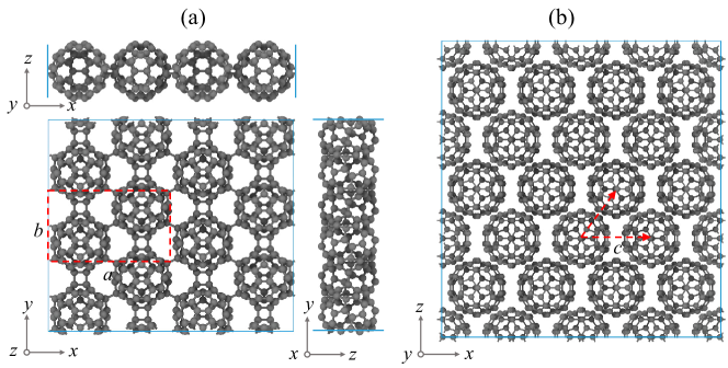
Figure 1: Crystal structure of (a) monolayer QHPF and (b) BPF. The primitive cell of QHPF is formed by the lattice parameters $a$ and $b$.

II Models and Methods

II.1 Models

II.1.1 The crystal structure of quasi-hexagonal-phase fullerene

The crystal structure of monolayer QHPF is schematically shown in Fig. 1(a). The dashed lines represent the primitive cell containing two C₆₀ molecules with $120$ carbon atoms in total. Each C₆₀ molecule is linked with six neighbouring ones by covalent bonds, with the $[2+2]$ cycloaddition of ${}^{\prime}5,6^{\prime}$ bonds occurring along the $[010]$ direction and the C-C single-bonds forming along both the $[110]$ and $[1\overline{1}0]$ directions. Experimentally, 30-80 $\mu$m monolayer QHPF sheets have been exfoliated [15], demonstrating the thermal stability of this unique structure.

II.1.2 The crystal structure of bulk-phase fullerene

We will comparably study the BPF structure, which is schematically shown in Fig. 1(b). In this structure, each C₆₀ molecule occupies a site of the FCC lattice. There is no clear covalent bonds between the C₆₀ molecules. Actually, the C₆₀ molecules do not have fixed orientations but rotate constantly at room temperature.

II.2 The NEP approach for machine-learned potential

The NEP approach for MLP has been recently proposed [20] as a promising tool to study heat transport with high accuracy and low cost. It has been improved later [21, 22] and the version we used in this paper is the NEP3 model as detailed in Ref. [22].

For a MLP, the descriptor [25] is the most important aspect. In NEP3, the descriptor consists of a number of radial and angular components as described below.

The radial descriptor components are constructed as

$$q^{i}_{n}=\sum_{j\neq i}g_{n}(r_{ij})\quad\text{with}\quad 0\leq n\leq n_{\mathrm{max}}^{\mathrm{R}},$$ (1)

where the summation runs over all the neighbors of atom $i$ within a certain cutoff distance.

For the angular descriptor components, we consider both 3-body ones ($0\leq n\leq n_{\mathrm{max}}^{\mathrm{A}}$, $1\leq l\leq l_{\mathrm{max}}^{\mathrm{3b}}$)

$$q^{i}_{nl}=\sum_{m=-l}^{l}(-1)^{m}A^{i}_{nlm}A^{i}_{nl(-m)},$$ (2)

and 4-body ones ($0\leq n\leq n_{\mathrm{max}}^{\mathrm{A}}$, $1\leq l_{1}=l_{2}=l_{3}\leq l_{\mathrm{max}}^{\mathrm{4b}}$)

$$q^{i}_{nl_{1}l_{2}l_{3}}= \sum_{m_{1}=-l_{1}}^{l_{1}}\sum_{m_{2}=-l_{2}}^{l_{2}}\sum_{m_{3}=-l_{3}}^{l_{3}}\left(\begin{array}[]{ccc}l_{1}&l_{2}&l_{3}\\ m_{1}&m_{2}&m_{3}\\ \end{array}\right)$$ (5)

$$\times A^{i}_{nl_{1}m_{1}}A^{i}_{nl_{2}m_{2}}A^{i}_{nl_{3}m_{3}}.$$ (6)

Here,

$$A^{i}_{nlm}=\sum_{j\neq i}g_{n}(r_{ij})Y_{lm}(\theta_{ij},\phi_{ij}),$$ (7)

and $Y_{lm}(\theta_{ij},\phi_{ij})$ are the spherical harmonics as a function of the polar angle $\theta_{ij}$ and the azimuthal angle $\phi_{ij}$ for the position difference $\bm{r}_{ij}\equiv\bm{r}_{j}-\bm{r}_{i}$ from atom $i$ to atom $j$. The 4-body descriptor components have been inspired by the atomic cluster expansion (ACE) approach [26].

The functions $g_{n}(r_{ij})$ in Eq. (1) are defined as a linear combination of $N_{\mathrm{bas}}^{\mathrm{R}}+1$ basis functions $\{f_{k}(r_{ij})\}_{k=0}^{N_{\mathrm{bas}}^{\mathrm{R}}}$:

$$g_{n}(r_{ij}) =\sum_{k=0}^{N_{\mathrm{bas}}^{\mathrm{R}}}c^{ij}_{nk}f_{k}(r_{ij}),\quad\text{with}$$ (8)

$$f_{k}(r_{ij}) =\frac{1}{2}\left[T_{k}\left(2\left(r_{ij}/r_{\mathrm{c}}^{\mathrm{R}}-1\right)^{2}-1\right)+1\right]f_{\mathrm{c}}(r_{ij}).$$ (9)

Here, $T_{k}(x)$ is the $k^{\rm th}$ order Chebyshev polynomial of the first kind and $f_{\mathrm{c}}(r_{ij})$ is the cutoff function defined as

$$f_{\mathrm{c}}(r_{ij})=\begin{cases}\frac{1}{2}\left[1+\cos\left(\pi\frac{r_{ij}}{r_{\mathrm{c}}^{\mathrm{R}}}\right)\right],&r_{ij}\leq r_{\mathrm{c}}^{\mathrm{R}};\\ 0,&r_{ij}>r_{\mathrm{c}}^{\mathrm{R}}.\end{cases}$$ (10)

Here, $r_{\mathrm{c}}^{\mathrm{R}}$ is the cutoff distance of the radial descriptor components. The trainable expansion coefficients $c_{nk}^{ij}$ depend on $n$ and $k$ and also on the types of atoms $i$ and $j$. The functions $g_{n}(r_{ij})$ in Eq. (2) and Eq. (6) are defined similarly but with a different basis size $N_{\rm bas}^{\rm A}$ and a different cutoff distance $r_{\rm c}^{\rm A}$.

The various descriptor components are grouped into a vector with $N_{\mathrm{des}}$ components, $\{q^{i}_{\nu}\}_{\nu=1}^{N_{\mathrm{des}}}$. This vector is then taken as the input layer of a feedforward neural-network with a single hidden layer with $N_{\mathrm{neu}}$ neurons. The output of the neural network is taken as the potential energy of atom $i$. For the activation function in the hidden layer, we used the hyperbolic tangent function.

Although the neural network architecture is not different from the one as first proposed by Behler and Parrinello [27], the neural network in NEP is trained using a novel evolutionary algorithm called the separable natural evolution strategy (SNES) [28]. The loss function guiding the training process is defined as a weighted sum of the root mean square errors (RMSEs) of energy, force, and virial as well as terms serving as $\ell_{1}$ and $\ell_{2}$ regularization. The weighting factors for these terms are denoted as $\lambda_{\mathrm{e}}$, $\lambda_{\mathrm{f}}$, $\lambda_{\mathrm{v}}$, $\lambda_{1}$, and $\lambda_{2}$, respectively.

II.3 The homogeneous nonequilibrium molecular dynamics method

We used the HNEMD method to compute the thermal conductivity in a given system. This method was first formulated in terms of two-body potentials [29] and later generalized to many-body ones [24], including MLPs with atom-centered descriptors [20]. In this method, an external driving force (with zero net force) is added to the atoms in the system, leading to a heat current that has nonzero ensemble average (taken as time average in MD simulation) $\langle\bm{J}\rangle$. In the linear-response regime, the heat current is proportional to the driving force parameter $\bm{F}_{\rm e}$:

$$\langle J^{\alpha}\rangle=TV\sum_{\beta}\kappa^{\alpha\beta}F_{\rm e}^{\beta},$$ (11)

where $T$ is the temperature and $V$ is the volume of the system. The proportionality constant $\kappa^{\alpha\beta}$ is the $\alpha\beta$ component of the thermal conductivity tensor. In this paper, we are only interested in diagonal principal components of the thermal conductivity tensor. Then in a given direction $\alpha$, the thermal conductivity component is written as $\kappa^{\alpha}\equiv\kappa^{\alpha\alpha}$ and is computed as

$$\kappa^{\alpha}=\frac{\langle J_{\alpha}\rangle}{TVF_{\rm e}^{\alpha}}.$$ (12)

The heat current can be resolved in the frequency domain, leading to the spectral thermal conductivity [24]

$$\kappa^{\alpha}(\omega)=\frac{2}{VTF_{\rm e}^{\alpha}}\int_{-\infty}^{\infty}\text{d}te^{\text{i}\omega t}\sum_{i}\sum_{j\neq i}\left\langle r^{\alpha}_{ij}\frac{\partial U_{j}}{\partial\bm{r}_{ji}}(0)\cdot\bm{v}_{i}(t)\right\rangle.$$ (13)

Here, $U_{j}$ is the site energy of atom $j$, $\bm{r}_{ji}=\bm{r}_{i}-\bm{r}_{j}$, $\bm{r}_{i}$ is the position of atom $i$, and $\bm{v}_{i}$ is the velocity of atom $i$.

To cross check the HNEMD results, we also calculated the thermal conductivity of the QHPF structure using the Green-Kubo relation in the equilibrium molecular dynamics (EMD) method: [30, 31]

$$\kappa^{\alpha}=\frac{1}{k_{\rm B}T^{2}V}\int_{0}^{\infty}d\tau\langle J_{\alpha}J_{\alpha}(\tau)\rangle,$$ (14)

where $k_{\rm B}$ is Boltzmann’s constant and

$$J_{\alpha}=\sum_{i}\sum_{j\neq i}r^{\alpha}_{ij}\frac{\partial U_{j}}{\partial\bm{r}_{ji}}\cdot\bm{v}_{i}$$ (15)

is the heat current that is applicable to general many-body potentials [32].

In all the MD simulations, the time step for integration was set to 0.5 fs, the target temperature is 300 K and the target pressure is zero. In the HNEMD simulations the magnitude of the driving force parameter was chosen as $F_{\rm e}=0.5$ $\rm\mu m^{-1}$ and $F_{\rm e}=0.1$ $\rm\mu m^{-1}$ for BPF and QHPF, respectively. For BPF, we have performed three independent HNEMD simulations, each with a production time of 2 ns. For QHPF, we have performed five independent HNEMD simulations, each with a production time of 5 ns. For the EMD method, we have performed 60 independent simulations, each with a production time of 5 ns. The layer thickness of QHPF was set to 8.785 Å, which is the distance between two layers in bulk QHPF [15].

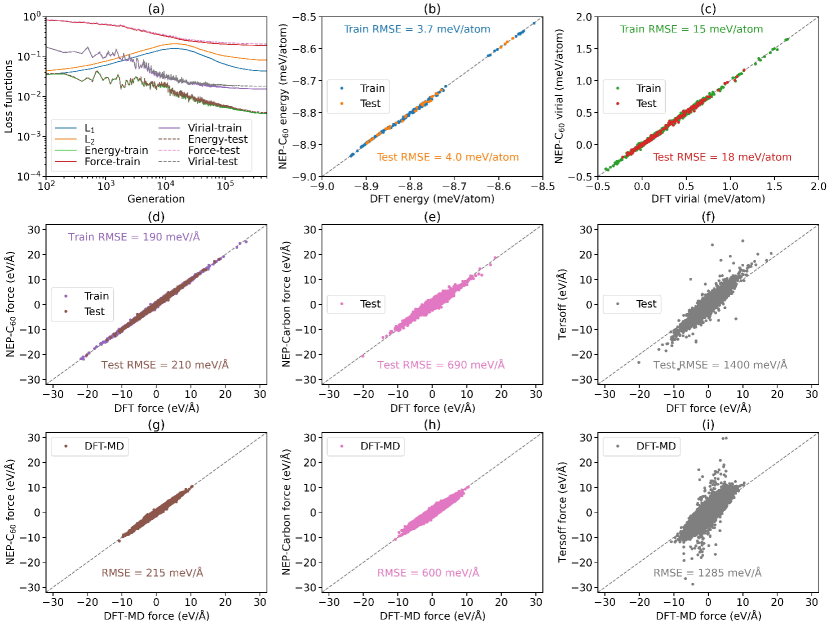
Figure 2: (a) Evolution of the various terms in the loss function for the training and testing data sets with respect to the generation. (b) Energy, (c) virial, and (d) force calculated from NEP-C₆₀ as compared to the DFT reference data for the training and testing data sets. Force calculated from (e) NEP-Carbon and (f) Tersoff as compared to the DFT reference data for the testing data set. Force calculated from (g) NEP-C₆₀, (h) NEP-Carbon and (i) Tersoff as compared to the DFT-MD reference values in the extra testing data set (1000 structures).

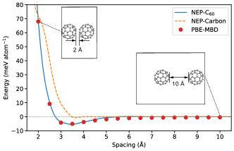
Figure 3: Energy of a linear chain of C₆₀ molecules as a function of the inter-molecular spacing.

III Results and Discussion

III.1 Training and validating the new NEP model

A NEP model for carbon systems has been recently trained [22], but the training data were mostly consisting of diamond, graphite, amorphous, and liquid structures, without explicit C₆₀ structures [33]. Both the QHPF and the BPF structures are stable in MD simulations with this NEP model, but as we will show later, this NEP model does not have sufficiently high accuracy for the QHPF and BPF structures. To ensure high accuracy in the MD simulations, we develop a more accurate NEP model trained against QHPF and BPF structures with DFT reference values. For clarity, we call the old and new NEP models NEP-Carbon and NEP-C₆₀, respectively.

III.1.1 Generation of training and testing structures

The training and testing structures include QHPF structures, BPF structures, and C₆₀ chains.

For QHPF, we used the NEP-Carbon model [22] to run $NpT$ (constant number of atoms $N$, controlled pressure $p$, and controlled temperature $T$) simulations with a rectangular box containing 120 carbon atoms. The Bussi-Donadio-Parrinello thermostat [34] and the Bernetti-Bussi barostat [35] were used to realize the $NpT$ ensemble. We considered three target pressures: 0, 1, and $-1$ GPa in both the $x$ and $y$ directions. For each target pressure, we linearly increased the target temperature from 10 K to 1000 K during a simulation time of 2,500 ps. We sampled the structures every 50 ps, obtaining 50 structures for each target pressure. Therefore, we have collected 150 structures in total. We used 120 randomly selected structures for training and the remaining 30 for testing. Apart from the above, we also performed DFT-based MD simulations at 800 K for 10 ps and sampled 1000 structures (each containing 240 atoms) to be used as an extra testing data set.

For BPF, we started from an ideal FCC unit cell with four C₆₀ molecules, which contains 240 carbon atoms in total. The centers of two neighboring C₆₀ molecules are separated by 9 Å [6]. We then applied perturbations with $3\%$ random box deformations and $0.1$ Å random atom displacements to create 15 training structures and 4 testing ones.

For C₆₀ chains, we considered two C₆₀ molecules in a box with vacuum in the transverse directions and varied the separation between them from 2 to 10 Å, with an interval of 0.5 Å, obtaining 17 structures in total. All these structures were used for training.

In summary, we have 152 and 1034 structures in the training and testing data sets, which contain 20,040 and 244,560 atoms, respectively. We have checked the learning curve to confirm that this training data set is large enough.

III.1.2 DFT calculations

After obtaining the structures, we used quantum-mechanical DFT calculations to obtain their reference energy, force, and virial data. To this end, we used the vasp package [36] and the PBE functional [37] combined with the many-body dispersion correction [38]. The energy cutoff for the projector augmented wave [39, 40] was chosen as 650 eV. A $\Gamma$-centered $k$-point mesh with a density of $0.25$ Å^-1, and a threshold of $10^{-8}$ eV were used for the electronic self-consistent loop. A Gaussian smearing with a width of 0.1 eV was used.

III.1.3 Choosing the training hyperparameters

After calculating the reference values, we used the gpumd package [23, 22] to train the NEP-C₆₀ model. The hyperparameters we chose are listed in Table 1. Compared to the hyperparameter values for the NEP-Carbon model [22], we have the following modifications. First, we have increased the radial cutoff from 4.2 to 7 Å and increased the angular cutoff from 3.7 to 4 Å. The notable increase in the radial cutoff is justified by the need for accurately describing the vdW interactions between the C₆₀ molecules, as will be further discussed below. Second, we have removed the 5-body descriptor components as defined in Ref. [22], which are not very important for our system. Third, we have increased the $\ell_{1}$ and $\ell_{2}$ regularization weights from 0.05 to 0.1, which can help to increase the robustness of the potential in MD simulations. Fourth, we have increased the virial weight in the loss function from 0.1 to 0.5, because virial has been regarded to be important for heat transport applications [41].

Table 1: Hyperparameters for the NEP-C₆₀ model.

parameter	value	parameter	value
$r_{\rm c}^{\rm R}$	7 Å	$r_{\rm c}^{\rm A}$	4 Å
$n_{\rm max}^{\rm R}$	10	$n_{\rm max}^{\rm A}$	8
$N_{\rm bas}^{\rm R}$	10	$N_{\rm bas}^{\rm A}$	8
$l_{\rm max}^{\rm 3b}$	4	$l_{\rm max}^{\rm 4b}$	2
$N_{\rm neu}$	50	$\lambda_{1}$	0.1
$\lambda_{2}$	0.1	$\lambda_{\rm e}$	1.0
$\lambda_{\rm f}$	1.0	$\lambda_{\rm v}$	0.5
$N_{\rm bat}$	10000	$N_{\rm pop}$	60
$N_{\rm gen}$	$5\times 10^{5}$

III.1.4 Training and testing results

Figure 2(a) shows the evolution of the various components in the loss function during the training process. The training has been performed for $5\times 10^{5}$ generations, after which the predicted energy, virial, and force are compared against the DFT reference values in Figs. 2(b)-2(d) and 2(g). The RMSEs of the various quantities for both the training data set and the hold-out testing data set are presented. As a comparison, we also show the parity plots of force for the NEP-Carbon model and the Tersoff potential in Figs. 2(e), 2(f), 2(h), and 2(i). We see that the current NEP model exhibits a much higher accuracy compared to the other two potential models. Our NEP-C₆₀ model can also accurately describe the interaction energy between the C₆₀ molecules in the linear chain structure with different inter-molecular distances, as shown in Fig. 3. The vdW interactions between the C₆₀ molecules are mostly captured by the radial descriptor components with a relatively long cutoff (7 Å) in our NEP model. In other MLPs, vdW interactions in carbon systems have been modelled by an explicit dispersion term with [42] or without [43, 44] environment dependence.

Table 2: Lattice constants of monolayer QHPF as calculated by the various potentials as well as DFT.

Model	$a$ (Å)	$b$ (Å)
DFT	15.81	9.12
NEP-C60	15.79	9.14
NEP-Carbon	15.88	9.18
Tersoff	16.30	9.35

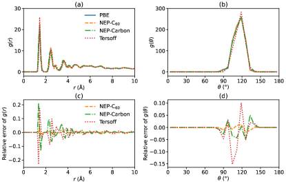
Figure 4: The (a) radial and (b) angular distribution functions of the QHPF structure at 800 K from DFT-PBE and the three potentials. The relative errors of the predictions by the three potentials to the DFT-PBE results for the (c) radial and (d) angular distribution functions.

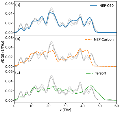
Figure 5: The vibrational density of states of the QHPF structure at 800 K calculated using the (a) NEP-C₆₀ model, (b) the NEP-Carbon model, and (c) the Tersoff potential. Due to the high computational cost for DFT-PBE, we show the results from five short trajectories (represented as five thin lines in each subplot) to emphasize its relatively large statistical errors. For the three classical potential models, we have used long trajectories and the results have negligible statistical errors which are thus not shown for clarity.

To further demonstrate the higher accuracy of the NEP-C₆₀ model compared to the NEP-Carbon model and the Tersoff potential, we compare the lattice constants in Table 2. The lattice constants calculated from the NEP-C₆₀ model agree with the DFT values with less than $0.1\%$ errors. The NEP-Carbon model has a little larger but still acceptable errors, but the Tersoff potential has 2-3 % errors. Figures 4 and 5 show that the NEP-C₆₀ model also has higher accuracy than the other two for radial distribution, angular distribution, and vibrational density of states. We expect that the higher accuracy of the NEP-C₆₀ model can lead to more reliable prediction of the physical properties as discussed in the remainder of this paper.

III.2 Thermal transport

III.2.1 The bulk-phase fullerene crystal

Figures 6(a)-6(c) show the cumulative time-average of the thermal conductivity as computed using Eq. (12) for the BPF structure at 300 K. A cubic simulation cell with 30,000 atoms was used. Apart from the NEP-C₆₀ potential model constructed in this work, we also considered the old NEP-Carbon model [22] and a hybridized potential formed by an intra-molecular Tersoff potential [19] and an inter-molecular Lennard-Jones (LJ) potential, which we call the Tersoff-LJ potential. The energy and length parameters in the LJ potential was chosen as $\epsilon=$ 2.86 meV and $\sigma=$ 3.47 Å [45]. The time-converged thermal conductivity is presented in Fig. 6(d) and Table 3.

Table 3: Thermal conductivity $\kappa$ (in units of W/mK) of BPF and QHPF (in the $x$ and $y$ directions) as calculated by NEP-Carbon, NEP-C₆₀, Tersoff and from experiments. An LJ potential is added to the Tersoff potential in the case of BPF. The experimental value is taken from Ref. [3]

Method		QHPF-$x$	QHPF-$y$	BPF
HNEMD	Tersoff	$75(9)$	$173(7)$	$0.14(6)$
	NEP-Carbon	$34(1)$	$37(2)$	$1.6(3)$
	NEP-C60	$102(3)$	$137(7)$	$0.45(5)$
EMD	NEP-C60	$109(19)$	$138(18)$	NA
Experiment		NA	NA	$\sim 0.4$

The thermal conductivity of BPF at 300 K has been measured to be about $0.4$ W/mK [3]. The Tersoff-LJ potential gives $0.14(6)$ W/mK, which is much smaller than the experimental value. The NEP-Carbon model gives $1.6(3)$ W/mK, which is much larger than the experimental value. The NEP-C₆₀ model, on the other hand, gives $0.45(5)$ W/mK, which is very close to the experimental value. Moreover, the fast rotation of the C₆₀ molecules in BPF as observed experimentally [3] can been reproduced with the NEP-C₆₀ model (see the Supplementary Material for movies of the trajectories during the MD simulations of BPF as well as QHPF) but not with the NEP-Carbon model. After confirming the reliability of the NEP-C₆₀ model in the prediction of the thermal conductivity of BPF, we next study heat transport in the new QHPF structure.

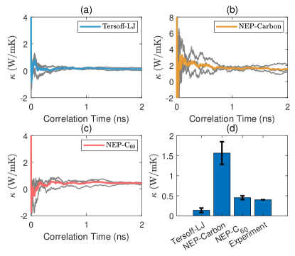
Figure 6: Thermal conductivity as a function of time for BPF at 300 K calculated using the HNEMD method with (a) the Tersoff-LJ potential, (b) the NEP-Carbon model, and (c) the NEP-C₆₀ model. (d) The converged thermal conductivity values from the different potentials as compared to an experiment value [3].

III.2.2 The monolayer quasi-hexagonal-phase fullerene

We similarly calculated the thermal conductivity of the QHPF structure at 300 K using the three potential models. A rectangular cell with 28,800 atoms was used, which is large enough to eliminate finite-size effects in the HNEMD method. The results are shown in Fig. 7 and Table 3. As a cross-check, we also calculated the thermal conductivity of the QHPF structure at 300 K using the EMD method (with the same simulation domain size as in HNEMD). The results are shown in Fig. 8 and Table 3. We see that the results from EMD and HNEMD are consistent in both the $x$ and $y$ directions within the statistical error bounds.

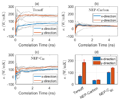
Figure 7: Thermal conductivity as a function of time for the QHPF structure at 300 K calculated using the HNEMD method with (a) the Tersoff potential, (b) the NEP-Carbon model, and (c) the NEP-C₆₀ model. (d) The converged thermal conductivity values from the different potentials.

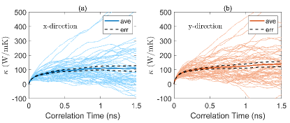
Figure 8: The running thermal conductivity as a function of the correlation time for the QHPF structure at 300 K in the (a) $x$ and (b) $y$ directions calculated using the EMD method with the NEP-C₆₀ potential. In each subplot, the thin lines represent the results from 60 individual runs (each with 5 ns production time), and the thick solid and dashed lines represent their average and error bounds.

Different from BPF, which is essentially isotropic regarding heat transport, it turns out that heat transport in QHPF is anisotropic. The thermal conductivity in the $y$ direction (see Fig. 1) is about 40% higher than that in the $x$ direction according to the NEP-C₆₀ potential. The $x$ and $y$ components of the thermal conductivity in QHPF are about 200 and 300 times of that of BPF. The NEP-Carbon potential predicted a much smaller anisotropy while the Tersoff potential predicted a much larger one. Based on the results for BPF, we expect that the NEP-C₆₀ potential gives the most reliable predictions due to its superior accuracy for the C₆₀-based structures. Nevertheless, we stress that the thermal conductivity of QHPF has not been experimentally measured so far and out results here should be regarded as theoretical predictions.

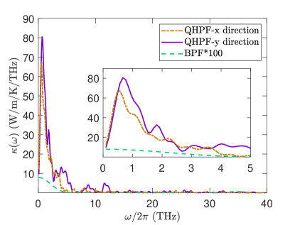
Figure 9: The spectral thermal conductivity as a function of the vibrational frequency for QHPF in the $x$ and $y$ directions and BPF calculated using the NEP-C₆₀ potential. Note that we have multiplied the $\kappa(\omega)$ for BPF by 100. The inset shows the part with $\omega/2\pi<5$ THz.

Figure 10: (a) Phonon dispersion relations and (b) phonon group velocities in QHPF. We have omitted frequencies above 20 THz for clarity. The small negative frequencies around the $\Gamma$ point in (a) are typical for the frozen-phonon approach we used. More advanced methods that take finite-temperature effects into account can help to alleviate this numerical problem.

To gain more insight, we show the spectral thermal conductivity $\kappa(\omega)$ of QHPF in the $x$ and $y$ directions and that of BPF in Fig. 9. We see that for all the materials and transport directions considered here, heat is mainly transported by phonons with frequency smaller than about $\nu=\omega/2\pi=2$ THz, which is almost the range for the acoustic phonon branches in QHPF (see Fig. 10(a)). This means that the acoustic phonons are the major heat carriers in QHPF. On the other hand, the phonon group velocities (see Fig. 10(b)) show relatively larger values for the $y$ direction (corresponding to the $\Gamma-Y$ path) than the $x$ direction (corresponds to the $\Gamma-X$ path). This can partially explain the anisotropic thermal conductivity in QHPF as group velocity is one of the major factors determining the thermal conductivity. Besides thermal conductivity, the in-plane elasticity in QHPF has also been found to be anisotropic [46]. The anisotropy as exhibited by these physical properties can be expected from the asymmetric inter-molecular bonding in QHPF as shown in Fig. 1.

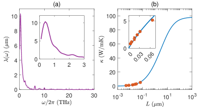
Figure 11: (a) The phonon mean free path $\lambda(\omega)$ as a function of the frequency for QHPF in the $x$ direction calculated using the NEP-C₆₀ potential. The inset shows the part with $\omega/2\pi<3$ THz. (b) The effective thermal conductivity $\kappa$ as a function of the system length $L$. The circles represent results from the NEMD simulations, and the line is from the HNEMD simulations. The inset shows the part with $L<80$ nm.

Using the methods as developed in Refs. [24] and [47], we also calculated the phonon mean-free path (MFP) spectrum $\kappa(\omega)$, as shown in Fig. 11(a). The low-frequency phonons develop MFPs up to about 10 microns, and the thermal conductivity thus only exhibits a convergence up to a system length (not to be confused with the simulation domain length in the HNEMD or EMD methods) of about one millimeter, as can be seen from Fig. 11(b). Due to the presence of the large MFPs, it is unfeasible to calculate the diffusive thermal conductivity using the non-equilibrium molecular dynamics (NEMD) method. However, agreement between NEMD and HNEMD can be observed in a range of system length that is affordable for our NEMD simulations.

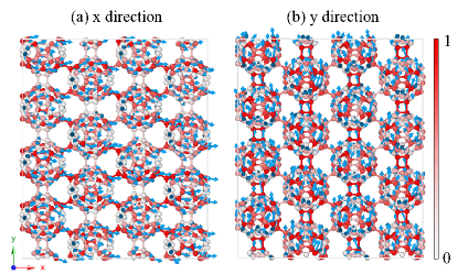
Figure 12: The per-atom heat current distribution in QHPF with heat transport in the (a) $x$ and (b) $y$ directions. The color on the atoms represents the normalized magnitude of the per-atom heat current in the transport direction. The arrow represents both the magnitude and the direction of the per-atom heat current. Only a small part of a system with 28,800 atoms is shown here for clarity.

Apart from the frequency and momentum spaces, insight can also be gained by from the real space. Figure 12 shows the real-space heat current distribution in the HNEMD simulations. When the transport direction is $x$, inter-molecular heat is mainly carried by the atoms forming the C-C single bonds between the molecules; when the transport direction is $y$, inter-molecular heat is mainly carried by the atoms forming the so-called $[2+2]$ cycloaddition bonds along the [010] direction [15]. For both directions, the inter-molecular heat is not mainly carried by the weak vdW interactions but by the strong covalent bonds. By contrast, there is no persistent inter-molecular covalent bond in BPF and the C₆₀ molecules rotate quickly, resulting in a strong suppression of the heat transport. This comparison highlights the vital role played by the inter-molecular covalent bonds in enhancing the thermal conductivity in QHPF as compared to that in BPF.

IV Summary and conclusions

In summary, we have constructed an accurate and transferable MLP based on the efficient NEP approach [20], which is applicable to both BPF and QHPF. The NEP model can accurately describe both the covalent bonding and the vdW interactions in the C₆₀ based structures. It predicted a thermal conductivity value of $0.45(5)$ W/mK at 300 K for BPF, which agrees with the experimental results [3] excellently. We then predicted the thermal conductivity of QHPF to be anisotropic and is more than two orders of magnitude higher than BPF. We find that the inter-molecular covalent bonding in QHPF plays a crucial role in enhancing the thermal conductivity in QHPF as compared to that in BPF. As a possible future direction of research, we note that the NEP-C₆₀ model developed here can be extended (by adding extra training data) to study multi-layer and three-dimensional structures of stacked QHPF as well as other polymerized structures based on C₆₀.

Data availability

Complete input and output files for the NEP training and testing are freely available at a Zenodo repository [48].