A Uniform Convergent Petrov-Galerkin method for a Class of Turning Point Problems

Abstract

In this paper, we propose a numerical method for turning point problems in one dimension based on Petrov-Galerkin finite element method (PGFEM). We first give a priori estimate for the turning point problem with a single boundary turning point. Then we use PGFEM to solve it, where test functions are the solutions to piecewise approximate dual problems. We prove that our method has a first-order convergence rate in both $L^{\infty}$ norm and an energy norm when we select the exact solutions to dual problems as test functions. Numerical results show that our scheme is efficient for turning point problems with different types of singularities, and the convergency coincides with our theoretical results.

5N06, 65B99.

1 Introduction

Singularly perturbed problems have been widely studied in the fields of fluid mechanics, aerodynamics, convection-diffusion process, etc. In such problems, there exist boundary layers or interior layers because a small parameter is included in the coefficient of the highest derivative. Consider the following singularly perturbed turning point problem in one dimension:

$$\left\{\begin{aligned} &Lu=-\varepsilon u^{\prime\prime}+p(x)u^{\prime}+b(x)u=f(x),\quad x_{L}<x<x_{R},\\ &u(x_{L})=u_{L},\quad u(x_{R})=u_{R},\\ \end{aligned}\right.$$ (1)

where $p(x)$ has zeros $z_{1}<z_{2}<\cdots<z_{m}$ on $[x_{L},x_{R}]$. We assume $p$, $b$, and $f$ to be sufficiently smooth. Furthermore, we suppose

$$b(x)-p^{\prime}(x)\geq\gamma_{0}>0$$ (2)

to ensure the well-posedness of the dual problems. Each zero of $p(x)$ is presumed to be a single root, i.e., $p^{\prime}(z_{i})\neq 0$.

From the asymptotic analysis, we know that there will be boundary/interior layers at some of $z_{i}$’s. Here we consider the following types of singularities:

1. Exponential boundary layers (singularly perturbed problems without turning points);

2. Cusp-like interior layers (interior turning point problems);

3. Boundary layers of other types (boundary turning point problems).

Singularly perturbed elliptic equations without turning points have been widely studied by researchers. Various numerical methods are utilized, where finite difference methods and finite element methods play prominent roles. El-Mistikawy and Werle raise an exponential box scheme ⁸(EMW scheme) in order to solve Falkner-Skan equations. Kellogg, Berger, and Han², Riordan and Stynes²⁸, etc., find this EMW scheme efficient when solving singularly perturbed elliptic equations. Fitted operator numerical methods, such as exponentially fitted finite difference method and Petrov-Galerkin method, are developed. Another class of methods, fitted mesh methods^{12; 31; 16; 20; 6}, show good adaptivity to different problems, while remeshing is necessary in some moving front problems.

A turning point problem is a class of equations in which the coefficient $p(x)$ vanishes in the domain. Compared to singularly perturbed equations without turning points, interior layers and other types of boundary layers might appear in the solutions to turning point problems. O’Malley²⁵ and Abrahamson¹ analyze turning point problems in some common cases. Kellogg, Berger, and Han² theoretically examine turning point problems with single interior turning points, and they use a modified EMW scheme, which obtains a first-order (or lower) convergence rate. Stynes and Riordan ^{28; 29} build a numerical scheme under Petrov-Galerkin framework and prove the uniform convergence in $L^{1}$ norm and $L^{\infty}$ norm. Farrell⁹ proposes sufficient conditions for an exponentially fitting difference scheme to be uniformly convergent for a turning point problem. Farrell and Gartland¹⁰ modify the EMW scheme and construct a scheme with uniform first-order convergency, where parabolic cylinder functions are used in the computation. For other studies of turning point problems using fitted operator methods, please refer to ^{27; 34; 11; 21}; for fitted mesh methods, please refer to ^{30; 22; 5; 26; 24; 19; 36}.

We notice that most of the present research assume turning points to be away from the boundary. If a turning point meets an endpoint, the problem is called a boundary turning point problem, which has not been thoroughly studied. In ³³, Vulanović considers a turning point problem with an arbitrary single turning point and obtains uniform convergency using finite difference method on a non-equidistant mesh. Vulanović and Farrell³⁵ examine a multiple boundary turning point problem and make priori estimates. However, estimates for single boundary turning point problems and numerical methods based on the uniform mesh are not given yet. In order to fill this blank, in this paper we estimate the derivatives of the solution to a standard single boundary turning point problem and raise an algorithm without particular mesh generation.

Petrov-Galerkin finite element method (PGFEM) is used in many problems. Dated back to 1979, Hemker and Groen⁷ raise a method that treats problem (1) with Petrov-Galerkin method, where the coefficient $p(x)$ has a positive lower bound. The scheme in Farrell and Gartland ¹⁰ is based on the so-called patched function method, also interpreted as Petrov-Galerkin method. In references ^{3; 4}, Petrov-Galerkin method and discontinuous Petrov-Galerkin method are implemented in elliptic equations in two dimensions, demonstrating their efficiency and convergency.

Tailored Finite Point Method (TFPM) is raised by Han, Huang, and Kellogg¹⁵, which is designed to solve PDEs using properties of the solutions, especially for singularly perturbed problems. TFPM could handle exponential singularities well, while simple difference methods might sometimes suffer from a low convergence rate. TFPM is later utilized in interface problems¹⁷, steady-state reaction-diffusion equations¹³, convection-diffusion-reaction equations¹⁴, etc.

This study presents a numerical scheme to solve problem (1) with several types of singularities. We prove that the width of the boundary layer of a single boundary turning point problem is $O(\sqrt{\varepsilon})$, which is a weaker version of the result in ³⁵. The derivative of the solution, $u^{\prime}$, is bounded by $C(1+\varepsilon^{-1/2})$ near the boundary layer and bounded by $C(1+x^{-1})$ away from the layer.

The rest of this paper is organized as follows. In section 2, priori estimates for continuous problems will be shown in each case. We use PGFEM to solve problem (1), where we choose (either exact or approximate) solutions to dual problems as test functions. We show details related to the numerical implementation in section 3. Numerical results demonstrate our scheme’s efficiency and the uniform first-order convergency in section 4. Finally, we give a brief conclusion in section 5.

2 A Priori estimate

In this section, we will present some priori estimates for cases (a)(b)(c) respectively. First we briefly recall some results from previous work for cases (a) and (b). We will prove our estimates for case (c) later.

2.1 Exponential boundary layer

Suppose the velocity coefficient $p(x)\geq p_{0}>0$ (or otherwise, it has a negative upper bound). Equation (1) is now written as:

$$\left\{\begin{aligned} &Lu\equiv-\varepsilon u^{\prime\prime}+p(x)u^{\prime}+b(x)u=f(x),\quad-1<x<1,\\ &u(-1)=u_{L},\quad u(1)=u_{R},\\ &p(x)\geq p_{0}>0,\quad b(x)\geq b_{0}\geq 0.\\ \end{aligned}\right.$$ (3)

The solution to (3) admits a boundary layer at $x=1$ (at $x=-1$ if $p(x)\leq p_{0}<0$), and it is shown^{18; 2} that the following estimates hold:

$$|u^{(k)}(x)|\leq C\Big{(}1+\varepsilon^{-k}\exp(-\frac{\eta(1-x)}{\varepsilon})\Big{)},\quad x\in(-1,1),\quad k=0,1,2,\cdots,$$ (4)

where $C,\eta$ are positive constants independent of $\varepsilon$. We have the following property at once:

Proposition 2.1.

Suppose $u$ is the solution to (3) and $p(x)$ is lower bounded, then there exists a constant $C$ independent of $\varepsilon$, such that

$$|(1-x)u^{\prime}(x)|\leq C,\quad\forall x\in(-1,1).$$ (5)

2.2 Cusp-like interior layer

Suppose there is only one turning point $x=0$, and equation (1) reads:

$$\left\{\begin{aligned} &Lu\equiv-\varepsilon u^{\prime\prime}+p(x)u^{\prime}+b(x)u=f(x),\quad-1<x<1,\\ &u(-1)=u_{L},\quad u(1)=u_{R},\\ &p(0)=0,p^{\prime}(0)<0,|p^{\prime}(x)|\geq\frac{1}{2}|p^{\prime}(0)|,\quad b(x)\geq b_{0}>0.\\ \end{aligned}\right.$$ (6)

In some papers, $x=0$ is called an attractive turning point because flows on both sides are toward the turning point, and (6) is called an attractive turning point problem. Such problems are characterized by the parameter $\lambda=-b(0)/p^{\prime}(0)$. It is shown^{1; 2} that the solution has an interior layer when $\lambda\in(0,1]$, and the following estimates hold:

$$|u^{(k)}(x)|\leq C\big{(}|x|+\sqrt{\varepsilon}\big{)}^{\lambda-k},\quad x\in(-1,1),\quad k=0,1,2,\cdots.$$ (7)

Similar to the previous case, the first derivative of the solution turns out bounded after multiplying a factor $x$:

Proposition 2.2.

Suppose $u$ is the solution to (6), then there exists a constant $C$ independent of $\varepsilon$, such that

$$|xu^{\prime}(x)|\leq C,\quad\forall x\in(-1,1),$$ (8)

on the assumption that $\lambda\in(0,1]$.

If $p^{\prime}(0)>0$, the problem is also called a repulsive turning point problem, and its solution is smooth near the turning point. Thus we need no additional treatment when dealing with such turning points.

2.3 Boundary turning point problem

Consider the turning point is positioned at an endpoint. We set the interval as $[0,1]$, and (1) becomes:

$$\left\{\begin{aligned} &Lu=-\varepsilon u^{\prime\prime}+p(x)u^{\prime}+b(x)u=f(x),\quad 0<x<1,\\ &u(0)=u_{L},\quad u(1)=u_{R},\\ &p(0)=0,|p^{\prime}(x)|\geq\frac{1}{2}|p^{\prime}(0)|,\quad b(x)\geq b_{0}>0.\\ \end{aligned}\right.$$ (9)

For multiple boundary turning point problems, i.e., $p^{(k)}(0)=0$ for $k=1,2,\cdots,m$, it is proved³⁵ that there exist positive constants $C,\eta$ independent of $\varepsilon$ such that the following estimates hold true:

$$|u^{(k)}(x)|\leq C\bigg{(}1+\varepsilon^{-k/2}\exp\big{(}-\frac{\eta x}{\sqrt{\varepsilon}}\big{)}\bigg{)},\quad x\in(0,1),\quad k=0,1,2,\cdots.$$ (10)

One can deduce the following result immediately:

$$|u^{(k)}(x)| \leq C\min\{(1+\varepsilon^{-k/2}),(1+x^{-k})\}$$ (11)

$$=C(1+(\max\{x,\sqrt{\varepsilon}\})^{-k}).$$

Now assume that the boundary turning point is single, i.e., $p^{\prime}(0)\neq 0$. Boundary behaviors of such problems differ from those of (3). We introduce the following approximated problem:

$$\left\{\begin{aligned} &\tilde{L}u\equiv-\varepsilon u^{\prime\prime}+p^{\prime}(0)xu^{\prime}+b(0)u=f(0),\quad 0<x<1,\\ &u(0)=u_{L},\quad u(1)=u_{R},\\ &p^{\prime}(0)\neq 0,\quad b(0)>0.\\ \end{aligned}\right.$$ (12)

We divide the discussion of problem (12) into two cases by the signal of $p^{\prime}(0)$. Inspired by ², we could represent the solution as a linear combination of Weber’s parabolic cylinder functions, which we use to analyze the bounds of the derivatives.

2.3.1 Preparations for estimates

We introduce a lemma to estimate the solution $u$ more precisely.

Lemma 2.3.

There exists one and only one solution $u$ to (9). Besides, there is a constant $C$ independent with $\varepsilon$, such that

$$|p(x)u^{\prime}(x)|\leq C,\quad\forall x\in[0,1/2].$$ (13)

Proof 2.4.

We suffice to show that $\varepsilon u^{\prime\prime}(x)$ is bounded by $C$ on $[0,1/2]$, for $u$ could be bounded by $f$ using the maximum principle. First assume that $p^{\prime}(0)=-\alpha<0$, and let $z(x)=u^{\prime\prime}(x)$. Differentiate (9) once, and we have:

$$-\varepsilon z^{\prime}+p(x)z=s(x),$$

where $s(x)=s_{1}(x)+s_{2}(x)$,

$$s_{1}(x)=f^{\prime}(x)-b^{\prime}(x)u,$$

$$s_{2}(x)=-(p^{\prime}(x)+b(x))u^{\prime}.$$

Let

$$P(x)=-\int_{0}^{x}p(t)dt.$$

Since

$$p^{\prime}(x)\leq-\frac{1}{2}\alpha<0,$$

it holds that:

$$p(x)\leq-\frac{1}{2}\alpha x\leq 0,$$

$$P(x)\geq\frac{\alpha}{4}x^{2}\geq 0.$$

Thus

$$-\frac{P(x)}{\varepsilon}\leq 0,$$

$$P(t)-P(x)=\int_{t}^{x}p(\tau)d\tau\leq 0,$$

for $0<t<x.$ By variance of constants we have

$$z(x)=z(0)\exp\Big{(}-\frac{P(x)}{\varepsilon}\Big{)}-\varepsilon^{-1}\int_{0}^{x}\exp\Big{(}\frac{P(t)-P(x)}{\varepsilon}\Big{)}s(t)dt.$$ (14)

Taking $x=0$ in (9),

$$z(0)=\varepsilon^{-1}(b(0)u(0)-f(0))=C\varepsilon^{-1}.$$

The integral in the second term of (14) is split into terms with $s_{1}$ and $s_{2}$:

$$I_{1}=\int_{0}^{x}\exp\Big{(}\frac{P(t)-P(x)}{\varepsilon}\Big{)}s_{1}(t)dt\leq\int_{0}^{x}1\cdot Cdt=C;$$

$$I_{2} =\int_{0}^{x}\exp\Big{(}\frac{P(t)-P(x)}{\varepsilon}\Big{)}s_{2}(t)dt$$

$$=-\int_{0}^{x}\exp\Big{(}\frac{P(t)-P(x)}{\varepsilon}\Big{)}\Big{(}p^{\prime}(t)+b(t)\Big{)}u^{\prime}(t)dt$$

$$=-\exp\Big{(}\frac{P(t)-P(x)}{\varepsilon}\Big{)}\Big{(}p^{\prime}(t)+b(t)\Big{)}u(t)\bigg{|}_{t=0}^{t=x}$$

$$\quad+\int_{0}^{x}\exp\Big{(}\frac{P(t)-P(x)}{\varepsilon}\Big{)}\Big{(}p^{\prime\prime}(t)+b^{\prime}(t)\Big{)}u(t)dt$$

$$\quad+\int_{0}^{x}\frac{d}{dt}\Big{[}\exp\Big{(}\frac{P(t)-P(x)}{\varepsilon}\Big{)}\Big{]}\Big{(}p^{\prime}(t)+b(t)\Big{)}u(t)dt$$

$$\leq C+C+C\int_{0}^{x}\frac{d}{dt}\Big{[}\exp\Big{(}\frac{P(t)-P(x)}{\varepsilon}\Big{)}\Big{]}dt$$

$$=C,$$

where we use the second mean value theorem for integrals before the inequality. Thus we have shown that $\varepsilon u^{\prime\prime}(x)$ is bounded on $[0,1]$ if $p^{\prime}(0)<0$.

In the case $p^{\prime}(0)=\alpha>0$, the same argument could be repeated with the following modification:

$$z(x)=\exp\Big{(}\frac{P(\frac{1}{2})-P(x)}{\varepsilon}\Big{)}z\Big{(}\frac{1}{2}\Big{)}-\varepsilon^{-1}\int_{x}^{1/2}\exp\Big{(}\frac{P(\tau)-P(x)}{\varepsilon}\Big{)}s(\tau)d\tau,$$

where $|z(\frac{1}{2})|$ is bounded by $C$. The result here applies only for $x\in[0,\frac{1}{2}]$ because (9) has a boundary layer at $x=1$.

We have shown that $p(x)u^{\prime}(x)$ is bounded near the singular point $x=0$. The original problem (9) is solved by decomposing $u=u_{1}+u_{2}+u_{0}$:

$$u_{0}=\frac{f(0)}{b(0)},$$ (15)

$$\left\{\begin{aligned} &\tilde{L}u_{1}=0,\quad 0<x<1,\\ &u_{1}(0)=u_{L}-u_{0},\quad u_{1}(1)=u_{R}-u_{0},\\ \end{aligned}\right.$$

$$\left\{\begin{aligned} &\tilde{L}u_{2}=g(x),\quad 0<x<1,\\ &u_{2}(0)=u_{2}(1)=0,\\ \end{aligned}\right.$$

where $\tilde{L}$ is defined in (12), and

$$g(x)\equiv\big{(}f(x)-f(0)\big{)}-\big{(}p(x)-p^{\prime}(0)x\big{)}u^{\prime}-\big{(}b(x)-b(0)\big{)}u.$$

From Lemma 2.3 we could write

$$g(x)=h(x)x.$$

We solve $u_{1}$ by direct representation with parabolic cylinder functions, while $u_{2}$ is related to Green’s function for $\tilde{L}$.

2.3.2 Basic property of parabolic cylinder function

Parabolic cylinder functions $U(a,x),V(a,x)$, using Weber’s notations, are linear independent solutions to the equation:

$$-y^{\prime\prime}+\Big{(}a+\frac{x^{2}}{4}\Big{)}y=0,$$

where $a$ is a coefficient. The following properties will be used later:

$$\pi V(a,x)=\Gamma\Big{(}\frac{1}{2}+a\Big{)}\Big{(}\sin\pi a\cdot U(a,x)+U(a,-x)\Big{)};$$ (2.3.2.1)

$$\Gamma\Big{(}\frac{1}{2}+a\Big{)}U(a,x)=\pi\sec^{2}\pi a\Big{(}V(a,-x)-\sin\pi a\cdot V(a,x))\Big{)};$$ (2.3.2.2)

$$\sqrt{2\pi}U(a,ix)=\Gamma\Big{(}\frac{1}{2}-a\Big{)}\Big{(}e^{-i\pi(-\frac{a}{2}-\frac{1}{4})}U(-a,x)+e^{i\pi(-\frac{a}{2}-\frac{1}{4})}U(-a,-x)\Big{)};$$ (2.3.2.3)

$$U^{\prime}(a,x)+\frac{1}{2}xU(a,x)+\Big{(}a+\frac{1}{2}\Big{)}U(a+1,x)=0;$$ (2.3.2.4)

$$U^{\prime}(a,x)-\frac{1}{2}xU(a,x)+U(a-1,x)=0;$$ (2.3.2.5)

$$V^{\prime}(a,x)+\frac{1}{2}xV(a,x)-V(a+1,x)=0;$$ (2.3.2.6)

$$V^{\prime}(a,x)-\frac{1}{2}xV(a,x)-\Big{(}a-\frac{1}{2}\Big{)}V(a-1,x)=0;$$ (2.3.2.7)

$$U(a,x)=\exp\Big{(}-\frac{1}{4}x^{2}\Big{)}x^{-a-\frac{1}{2}}\delta_{1},\quad x\geq C_{0};$$ (2.3.2.8)

$$V(a,x)=\sqrt{\frac{2}{\pi}}\exp\Big{(}\frac{1}{4}x^{2}\Big{)}x^{a-\frac{1}{2}}\delta_{2},\quad x\geq C_{0}.$$ (2.3.2.9)

$C_{0}=O(1)$ is a constant related to $a$, and coefficients $\delta_{1},\delta_{2}$ satisfy

$$|\delta_{i}-1|\leq\frac{1}{3}.$$

2.3.3 Green’s function of the operator $\tilde{L}$

Denote $\mu_{0}$ by the solution to

$$\left\{\begin{aligned} &\tilde{L}u=0,\\ &u(0)=0,\quad u(1)=1,\\ \end{aligned}\right.$$

and $\mu_{1}$ by the solution to

$$\left\{\begin{aligned} &\tilde{L}u=0,\\ &u(0)=1,\quad u(1)=0.\\ \end{aligned}\right.$$

The Wronskian of $\mu_{0}$ and $\mu_{1}$ is

$$W(x)=W(\mu_{0},\mu_{1})=\mu_{0}(x)\mu_{1}^{\prime}(x)-\mu_{1}(x)\mu_{0}^{\prime}(x).$$

The Green’s function of $\tilde{L}$ is piecewise defined on $[0,1]$:

$$G(x,\tau)=\left\{\begin{aligned} &-\varepsilon^{-1}\mu_{0}(x)\mu_{1}(\tau)\exp\Big{(}\frac{p^{\prime}(0)}{2\varepsilon}(1-\tau^{2})\Big{)}/W(1),&0\leq x\leq\tau\leq 1,\\ &-\varepsilon^{-1}\mu_{1}(x)\mu_{0}(\tau)\exp\Big{(}\frac{p^{\prime}(0)}{2\varepsilon}(1-\tau^{2})\Big{)}/W(1),&0\leq\tau\leq x\leq 1,\\ \end{aligned}\right.$$

which satisfies

$$\tilde{L}G(x,\tau)=\delta(x-\tau),$$

$$G(0)=G(1)=0.$$

$u_{2}$ defined in (15) could be represented as

$$u_{2}(x)=\int_{0}^{1}G(x,\tau)\tau h(\tau)d\tau.$$

Thus estimates for $u_{2}$ turn into ones for $G(\cdot,\tau)$ and its derivatives.

2.3.4 The case $p^{\prime}(0)=\alpha>0$

We first estimate derivatives of the solution $u$ in the next lemma.

Lemma 2.5.

Assume $u$ is the solution to (9) with $p^{\prime}(0)>0$, and $\rho=C_{0}\sqrt{\varepsilon}$, where $C_{0}$ is defined in section 2.3.2. For $k=1,2,\cdots$,

$$|u^{(k)}(x)|\leq\left\{\begin{aligned} &C(1+\rho^{-k}),&0\leq x\leq\rho,\\ &C(1+x^{-k}),&\rho\leq x\leq 1/2.\\ \end{aligned}\right.$$ (16)

Rewriting these estimates in a more compact form, we have:

$$|u^{(k)}(x)|\leq C(1+(\max\{x,\rho\})^{-k}),\quad 0\leq x\leq 1/2.$$ (16’)

Proof 2.6.

Since $u_{0}$ in (15) has no contribution to the derivative, for the sake of simplicity, we replace $u$ by $u_{1}+u_{2}$ and still denote it by $u$. We introduce the following change of variable, for both $u_{1}$ and $u_{2}$ satisfy an equation of $\tilde{L}$:

$$\tilde{x}=\frac{x}{\sqrt{\varepsilon/\alpha}},$$

$$u(x)=\tilde{u}(\tilde{x})\exp\Big{(}\frac{\tilde{x}^{2}}{4}\Big{)}.$$

Denoting $\beta=b(0)/\alpha>0$, we obtain the equation for $\tilde{u}$:

$$-\tilde{u}^{\prime\prime}+\Big{(}\frac{\tilde{x}^{2}}{4}+\beta-\frac{1}{2}\Big{)}\tilde{u}=0.$$

$\tilde{u}$ admits linear independent solutions $U(\beta-\frac{1}{2},\tilde{x}),V(\beta-\frac{1}{2},\tilde{x})$. Hence

$$u(x)=c_{1}\exp\Big{(}\frac{\tilde{x}^{2}}{4}\Big{)}U\Big{(}\beta-\frac{1}{2},\tilde{x}\Big{)}+c_{2}\exp\Big{(}\frac{\tilde{x}^{2}}{4}\Big{)}V\Big{(}\beta-\frac{1}{2},\tilde{x}\Big{)}.$$

Coefficients $c_{1},c_{2}$ are determined by boundary conditions:

$$\left(\begin{array}[]{cc}U\Big{(}\beta-\frac{1}{2},0\Big{)}&V\Big{(}\beta-\frac{1}{2},0\Big{)}\\ \exp(\frac{\alpha}{4\varepsilon})U\Big{(}\beta-\frac{1}{2},\frac{1}{\sqrt{\varepsilon/\alpha}}\Big{)}&\exp(\frac{\alpha}{4\varepsilon})V\Big{(}\beta-\frac{1}{2},\frac{1}{\sqrt{\varepsilon/\alpha}}\Big{)}\\ \end{array}\right)\left(\begin{array}[]{c}c_{1}\\ c_{2}\\ \end{array}\right)=\left(\begin{array}[]{c}u_{L}\\ u_{R}\\ \end{array}\right).$$

Call the matrix on the left-hand-side $A$. Denoting $K_{i}$ as constants of $O(1)$, we could rewrite $A$ in the asymptotic form:

$$A\approx\left(\begin{array}[]{cc}K_{1}&K_{2}\\ K_{3}\varepsilon^{\beta/2}&K_{4}\exp(\frac{\alpha}{2\varepsilon})\varepsilon^{(1-\beta)/2}\\ \end{array}\right),$$

$$A^{-1}\approx\left(\begin{array}[]{cc}K_{4}&-K_{2}\exp(-\frac{\alpha}{2\varepsilon})\varepsilon^{(\beta-1)/2}\\ -K_{3}\exp(-\frac{\alpha}{2\varepsilon})\varepsilon^{\beta-1/2}&K_{1}\exp(-\frac{\alpha}{2\varepsilon})\varepsilon^{(\beta-1)/2}\\ \end{array}\right).$$

Therefore the coefficients are represented as follows:

$$\left(\begin{array}[]{c}c_{1}\\ c_{2}\\ \end{array}\right) =A^{-1}\left(\begin{array}[]{c}u_{L}\\ u_{R}\\ \end{array}\right).$$

We omit all the constants of $O(1)$ for simplicity. Considering $u_{L},u_{R}=O(1)$, the derivatives are in the following form:

$$u^{(k)}(x) =\varepsilon^{-k/2}\bigg{[}c_{1}\exp\Big{(}\frac{\tilde{x}^{2}}{4}\Big{)}\Pi^{k}_{i=1}(-\beta-i+1)U\Big{(}\beta+k-\frac{1}{2},\tilde{x}\Big{)}+c_{2}\exp\Big{(}\frac{\tilde{x}^{2}}{4}\Big{)}V\Big{(}\beta+k-\frac{1}{2},\tilde{x}\Big{)}\bigg{]}$$

$$=\varepsilon^{-k/2}\bigg{[}c_{1}^{\prime}\exp\Big{(}\frac{\tilde{x}^{2}}{4}\Big{)}U\Big{(}\beta+k-\frac{1}{2},\tilde{x}\Big{)}+c_{2}\exp(\frac{\tilde{x}^{2}}{4})V\Big{(}\beta+k-\frac{1}{2},\tilde{x}\Big{)}\bigg{]}.$$

For convenience, write $u_{1}(x)=u_{L}\mu_{1}(x)+u_{R}\mu_{0}(x)$, and we estimate $\mu_{0}$ and $\mu_{1}$ first in order to estimate $u_{1}$ and its derivatives on $[0,1/2]$:

$$|\mu_{0}^{(k)}(x)|\leq\left\{\begin{aligned} &C\exp(-\frac{\alpha}{2\varepsilon})\varepsilon^{\frac{\beta-k-1}{2}},&|x|\leq\rho,\\ &C\Big{(}\exp(-\frac{\alpha}{2\varepsilon})\varepsilon^{\beta-\frac{1}{2}}x^{-\beta-k}+\varepsilon^{-k}\exp\big{(}-\frac{\alpha}{2\varepsilon}(1-x^{2})\big{)}x^{\beta+k-1}\Big{)},&\rho\leq|x|\leq 1,\\ \end{aligned}\right.$$

$$|\mu_{1}^{(k)}(x)|\leq\left\{\begin{aligned} &C\varepsilon^{-\frac{k}{2}},&|x|\leq\rho,\\ &C\Big{(}\varepsilon^{\frac{\beta}{2}}x^{-\beta-k}+\exp\big{(}-\frac{\alpha}{2\varepsilon}(1-x^{2})\big{)}\varepsilon^{\frac{\beta}{2}-k}x^{\beta+k-1}\Big{)},&\rho\leq|x|\leq 1,\\ \end{aligned}\right.$$

which hold for $k=0,1,2,\cdots$. Thus

$$|W(1)|\geq C\varepsilon^{\beta/2-1}.$$

If $x\leq\rho$, from

$$u_{1}^{(k)}=u_{L}\mu_{1}^{(k)}+u_{R}\mu_{0}^{(k)},$$

we have:

$$|u_{1}^{(k)}(x)| \leq C\Big{(}|u_{R}||\mu_{0}^{(k)}(x)|+|u_{L}||\mu_{1}^{(k)}(x)|\Big{)}$$

$$\leq C\Big{(}|u_{R}|\exp(-\frac{\alpha}{2\varepsilon})\varepsilon^{\frac{\beta-k-1}{2}}+|u_{L}|\varepsilon^{-\frac{k}{2}}\Big{)},\quad k=1,2,\cdots.$$

If $\rho\leq x\leq 1/2$,

$$\exp(-\frac{\alpha}{2\varepsilon}(1-x^{2}))\leq\exp(-\frac{\alpha^{\prime}}{2\varepsilon}),$$

where $\alpha^{\prime}=\frac{3}{4}\alpha,$ we have

$$|u_{1}^{(k)}(x)| \leq C|u_{L}|\Big{(}\varepsilon^{\frac{\beta}{2}}x^{-\beta-k}+\exp\big{(}-\frac{\alpha}{2\varepsilon}(1-x^{2})\big{)}\varepsilon^{\frac{\beta}{2}-k}x^{\beta+k-1}\Big{)}$$

$$\quad+C|u_{R}|\Big{(}\exp(-\frac{\alpha}{2\varepsilon})\varepsilon^{\beta-\frac{1}{2}}x^{-\beta-k}+\varepsilon^{-k}\exp\big{(}-\frac{\alpha}{2\varepsilon}(1-x^{2})\big{)}x^{\beta+k-1}\Big{)}$$

$$\leq C(1+x^{-k}),\quad k=1,2,\cdots.$$

Constant $C$ may depend on $\beta,k,\alpha,C_{0}$. Derivatives of $u_{2}$ are estimated by induction.

$$|u_{2}^{\prime}(x)| \leq C\int_{0}^{1}|G_{x}(x,\tau)|\tau d\tau$$

$$=\left\{\begin{aligned} &\int_{0}^{x}+\int_{x}^{\rho}+\int_{\rho}^{1},&0\leq x\leq\rho,\\ &\int_{0}^{\rho}+\int_{\rho}^{x}+\int_{x}^{1},&\rho\leq x\leq\frac{1}{2}.\\ \end{aligned}\right.$$

Denote these six integrals as $I_{1,2,3}$ and $I_{1,2,3}^{\prime}$. The first three are easy to handle:
$I_{1}:0\leq\tau\leq x\leq\rho$:

$$|G_{x}|\leq C\varepsilon^{-1}\exp\Big{(}-\frac{\alpha}{2\varepsilon}\tau^{2}\Big{)},$$

$$I_{1}=\int_{0}^{x}|G_{x}|\tau d\tau\leq C.$$

$I_{2}:0\leq x\leq\tau\leq\rho$:

$$|G_{x}|\leq C\varepsilon^{-1}\exp\Big{(}-\frac{\alpha}{2\varepsilon}\tau^{2}\Big{)},$$

$$I_{2}=\int_{x}^{\rho}|G_{x}|\tau d\tau\leq C.$$

$I_{3}:0\leq x\leq\rho\leq\tau$:

$$|G_{x}|\leq C\Big{(}\varepsilon^{\frac{\beta}{2}-1}\exp(-\frac{\alpha}{2\varepsilon}\tau^{2})\tau^{-\beta}+\varepsilon^{\frac{\beta}{2}-1}\exp(-\frac{\alpha}{2\varepsilon})\tau^{\beta-1}\Big{)},$$

$$I_{3}=\int_{\rho}^{1}|G_{x}|\tau d\tau\leq C\int_{\rho}^{1}\exp\Big{(}-\frac{\alpha}{2\varepsilon}\tau^{2}\Big{)}\tau^{1-\beta}\varepsilon^{\frac{\beta-1}{2}}\varepsilon^{-\frac{1}{2}}d\tau+C\exp\Big{(}-\frac{\alpha}{2\varepsilon}\Big{)}\varepsilon^{\frac{\beta}{2}-1}$$

$$\quad\leq C\varepsilon^{-\frac{1}{2}}+C$$

$$\quad=C(1+\rho^{-1}).$$

Thus when $x\leq\rho$, we have

$$|u_{2}^{\prime}(x)|\leq C(1+\rho^{-1}).$$

For $x\geq\rho$, consider the last three integrals:
$I_{1}^{\prime}:0\leq\tau\leq\rho\leq x\leq\frac{1}{2}$:

$$|G_{x}| \leq\varepsilon^{\frac{\beta-1}{2}}\exp\Big{(}-\frac{\alpha}{2\varepsilon}\tau^{2}\Big{)}x^{-\beta-1}+\varepsilon^{\frac{\beta-1}{2}}x^{\beta}\exp\Big{(}-\frac{\alpha}{2\varepsilon}(1-x^{2})\Big{)}\exp\Big{(}-\frac{\alpha}{2\varepsilon}\tau^{2}\Big{)}\varepsilon^{-1}$$

$$\leq C\varepsilon^{-1}\exp\Big{(}-\frac{\alpha}{2\varepsilon}\tau^{2}\Big{)},$$

$$I_{1}^{\prime} =\int_{0}^{\rho}|G_{x}|\tau d\tau\leq C.$$

$I_{2}^{\prime}:\rho\leq\tau\leq x\leq\frac{1}{2}$:

$$|G_{x}| \leq\bigg{(}x^{-\beta-1}+\varepsilon^{-1}\exp\big{(}-\frac{\alpha}{2\varepsilon}(1-x^{2})\big{)}x^{\beta}\bigg{)}\bigg{(}\exp\big{(}-\frac{\alpha}{2\varepsilon}\tau^{2}\big{)}\varepsilon^{\beta-\frac{1}{2}}\tau^{-\beta}+\tau^{\beta-1}\bigg{)},$$

$$|G_{x}|\tau \leq\bigg{(}x^{-\beta-1}+\varepsilon^{-1}\exp\big{(}-\frac{\alpha}{2\varepsilon}(1-x^{2})\big{)}x^{\beta}\bigg{)}\bigg{(}\exp\big{(}-\frac{\alpha}{2\varepsilon}\tau^{2}\big{)}\varepsilon^{\beta-\frac{1}{2}}+\tau^{\beta}\bigg{)}$$

$$\leq\Big{(}x^{-\beta-1}+\varepsilon^{-1}\exp\big{(}-\frac{\alpha^{\prime}}{2\varepsilon}\big{)}\Big{)}\Big{(}C\varepsilon^{\frac{\beta}{2}}+\tau^{\beta}\Big{)},$$

$$I_{2}^{\prime} =\int_{\rho}^{x}|G_{x}|\tau d\tau\leq C(1+x^{-1}).$$

$I_{3}^{\prime}:\rho\leq x\leq\tau\leq 1,x\leq\frac{1}{2}$:

$$|G_{x}|\leq\bigg{(}\varepsilon^{\beta-\frac{1}{2}}\exp\big{(}-\frac{\alpha}{2\varepsilon}\big{)}x^{-\beta-1}+\varepsilon^{-1}\exp\big{(}-\frac{\alpha}{2\varepsilon}(1-x^{2})\big{)}x^{\beta}\bigg{)}$$

$$\quad\quad\quad\cdot\bigg{(}\exp\big{(}\frac{\alpha}{2\varepsilon}(1-\tau^{2})\big{)}\tau^{-\beta}+\tau^{\beta-1}\bigg{)},$$

$$I_{3}^{\prime}=\int_{x}^{1}|G_{x}|\tau d\tau\leq C(1+x^{-1}).$$

Therefore we have

$$|u_{2}^{\prime}(x)|\leq C(1+x^{-1}),$$

when $x\geq\rho$.

Considering that the behavior near $x=1$ has been studied well as an exponential boundary layer, we narrow down the priori estimate for $u$ to $[0,1/2]$:

$$|u^{\prime}(x)|\leq\left\{\begin{aligned} &C(1+\rho^{-1}),&0\leq x\leq\rho,\\ &C(1+x^{-1}),&\rho\leq x\leq 1/2.\\ \end{aligned}\right.$$

For higher derivatives $u^{(k)}(k\geq 2)$, we could differentiate $(k-1)$ times the equation in (9) and split $v=u^{(k-1)}$ into three parts as $u$ is decomposed in (15). It is noticed that $v$ satisfies a similar equation to (12), with $\beta$ replaced by $\beta+k-1$ and boundary conditions in asymptotic forms. Actually, we can obtain by induction, for $k=1,2,\cdots$:

$$u^{(k)}(0)=\varepsilon^{-\frac{k}{2}},$$

$$u^{(k)}(1)=\varepsilon^{-k}.$$

Simple calculations yield the following result:

$$|u^{(k)}(x)|\leq\left\{\begin{aligned} &C(1+\rho^{-k}),&0\leq x\leq\rho,\\ &C(1+x^{-k}),&\rho\leq x\leq 1/2.\\ \end{aligned}\right.$$

Remark 2.7.

If we take $x\approx 1$ into consideration, the estimates could be modified as:

$$|u^{(k)}(x)|\leq\left\{\begin{aligned} &C(1+\rho^{-k}),&0\leq x\leq\rho,\\ &C\Big{(}1+x^{-k}+(1-x)^{-k}\Big{)},&\rho\leq x\leq 1;\\ \end{aligned}\right.\quad k=1,2,\cdots.$$ (17)

Note that for $\frac{1}{2}\leq x\leq 1,$

$$\exp(-\frac{\alpha}{2\varepsilon}(1-x^{2}))\leq C(\frac{\varepsilon}{1-x})^{k}.$$

The following proposition holds as a direct conclusion, and we will use these propositions to show the convergence of the numerical method.

Proposition 2.8.

For the solution $u$ of (9), when $p^{\prime}(0)>0$, there exists a constant $C$, satisfying

$$|xu^{\prime}(x)|\leq C,\quad x\leq 1/2,$$ (18)

$$|(1-x)u^{\prime}(x)|\leq C,\quad x\geq 1/2.$$ (18’)

2.3.5 The case $p^{\prime}(0)=-\alpha<0$

In this case, estimates for derivatives of $u$ are mildly different.

Lemma 2.9.

Assume that $u$ is the solution to (9) when $p^{\prime}(0)<0$. Let $\beta=b(0)/\alpha>0$, and $\rho$ is defined as above. Then we have the following estimates:

$$|u^{(k)}(x)| \leq\left\{\begin{aligned} &C\Big{(}1+\rho^{\beta-k}+|u_{L}|\rho^{-k}\Big{)},&0\leq x\leq\rho,\\ &C\Big{(}1+x^{\beta-k}+|u_{L}|x^{-k}\Big{)},&\rho\leq x\leq 1;\\ \end{aligned}\right.\quad k=1,2,\cdots,$$ (19)

or otherwise in a compact form:

$$|u^{(k)}(x)|\leq C(1+(\max\{x,\rho\})^{\beta-k}+|u_{L}|(\max\{x,\rho\})^{-k}),\quad 0\leq x\leq 1,\quad k=1,2,\cdots.$$ (19’)

Proof 2.10.

If we let $\tilde{x}=\frac{x}{\sqrt{-\varepsilon/\alpha}}$, the new variable becomes pure imaginary. From the property that evaluation of $U(a,iz)$ and $V(a,iz)$ could be represented by $U(-a,z),V(-a,z)$ (c.f. (.1),(.3)), we assume the solution to be:

$$u(x)=c_{1}\exp\Big{(}\frac{\tilde{x}^{2}}{4}\Big{)}U\Big{(}\frac{1}{2}+\beta,|\tilde{x}|\Big{)}+c_{2}\exp\Big{(}\frac{\tilde{x}^{2}}{4}\Big{)}V\Big{(}\frac{1}{2}+\beta,|\tilde{x}|\Big{)}.$$

For simplicity we denote $\hat{x}=|\tilde{x}|=\frac{x}{\sqrt{\varepsilon/\alpha}}$, which gives:

$$u(x)=c_{1}\exp\Big{(}-\frac{\hat{x}^{2}}{4}\Big{)}U\Big{(}\frac{1}{2}+\beta,\hat{x}\Big{)}+c_{2}\exp\Big{(}-\frac{\hat{x}^{2}}{4}\Big{)}V\Big{(}\frac{1}{2}+\beta,\hat{x}\Big{)}.$$

Again we solve coefficients $c_{1},c_{2}$ from boundary conditions $u_{L},u_{R}$. Let

$$A =\left(\begin{array}[]{cc}U\Big{(}\frac{1}{2}+\beta,0\Big{)}&V\Big{(}\frac{1}{2}+\beta,0\Big{)}\\ \exp(-\frac{\alpha}{4\varepsilon})U\Big{(}\frac{1}{2}+\beta,\frac{1}{\sqrt{\varepsilon/\alpha}}\Big{)}&\exp(-\frac{\alpha}{4\varepsilon})V\Big{(}\frac{1}{2}+\beta,\frac{1}{\sqrt{\varepsilon/\alpha}}\Big{)}\\ \end{array}\right)$$

$$\approx\left(\begin{array}[]{cc}K_{1}&K_{2}\\ K_{3}\exp(-\frac{\alpha}{2\varepsilon})\varepsilon^{(1+\beta)/2}&K_{4}\varepsilon^{-\beta/2}\\ \end{array}\right).$$

The inverse of $A$ reads:

$$A^{-1} \approx\left(\begin{array}[]{cc}K_{4}&-K_{2}\varepsilon^{\beta/2}\\ -K_{3}\exp(-\frac{\alpha}{2\varepsilon})\varepsilon^{1/2+\beta}&K_{1}\varepsilon^{\beta/2}\\ \end{array}\right)$$

$$\approx C\left(\begin{array}[]{cc}1&\varepsilon^{\beta/2}\\ \exp(-\frac{\alpha}{2\varepsilon})\varepsilon^{1/2+\beta}&\varepsilon^{\beta/2}\\ \end{array}\right).$$

Then $c_{1},c_{2}$ could be written as

$$\left(\begin{array}[]{c}c_{1}\\ c_{2}\\ \end{array}\right) =A^{-1}\left(\begin{array}[]{c}u_{L}\\ u_{R}\\ \end{array}\right).$$

As the previous case, for $k=1,2,\cdots$,

$$u^{(k)}(x)=\varepsilon^{-k/2}\Big{[}c_{1}^{\prime}\exp\Big{(}-\frac{\hat{x}^{2}}{4}\Big{)}U\Big{(}\beta+\frac{1}{2}-k,\hat{x}\Big{)}+c_{2}^{\prime}\exp\Big{(}-\frac{\hat{x}^{2}}{4}\Big{)}V\Big{(}\beta+\frac{1}{2}-k,\hat{x}\Big{)}\Big{]}.$$

For $\mu_{0},\mu_{1}$, and $k=0,1,2,\cdots$,

$$\mu_{0}^{(k)}(x)=\exp\Big{(}-\frac{\hat{x}^{2}}{4}\Big{)}\varepsilon^{\frac{\beta-k}{2}}\bigg{(}U\Big{(}\beta+\frac{1}{2}-k,\hat{x}\Big{)}+V\Big{(}\beta+\frac{1}{2}-k,\hat{x}\Big{)}\bigg{)},$$

$$\mu_{1}^{(k)}(x)=\exp\Big{(}-\frac{\hat{x}^{2}}{4}\Big{)}\varepsilon^{-\frac{k}{2}}\bigg{(}U\Big{(}\beta+\frac{1}{2}-k,\hat{x}\Big{)}+\varepsilon^{\frac{1}{2}+\beta}\exp(-\frac{\alpha}{2\varepsilon})V\Big{(}\beta+\frac{1}{2}-k,\hat{x}\Big{)}\bigg{)}.$$

We have the following estimates:

$$\begin{aligned} &|\mu_{0}^{(k)}(x)|\leq\left\{\begin{aligned} &C\varepsilon^{\frac{\beta-k}{2}},&x\leq\rho,\\ &C\Big{(}\exp\big{(}-\frac{\alpha}{2\varepsilon}x^{2}\big{)}\varepsilon^{\beta+\frac{1}{2}-k}x^{-\beta+k-1}+x^{\beta-k}\Big{)},&x\geq\rho;\\ \end{aligned}\right.\\ &|\mu_{1}^{(k)}(x)|\leq\left\{\begin{aligned} &C\varepsilon^{-\frac{k}{2}},&x\leq\rho,\\ &C\Big{(}\exp\big{(}-\frac{\alpha}{2\varepsilon}x^{2}\big{)}\varepsilon^{\frac{\beta+1}{2}-k}x^{-\beta+k-1}+\exp(-\frac{\alpha}{2\varepsilon})\varepsilon^{\frac{\beta+1}{2}}x^{\beta-k}\Big{)},&x\geq\rho;\\ \end{aligned}\right.\end{aligned}\quad k=0,1,\cdots.$$

Since these two estimates are different from the case $p^{\prime}(0)>0$, we might keep $u_{L}$ and $u_{R}$ as independent variables.

$$|u_{1}^{(k)}(x)| \leq|u_{R}||\mu_{0}^{(k)}(x)|+|u_{L}||\mu_{1}^{(k)}(x)|$$

$$\leq\left\{\begin{aligned} &C\Big{(}|u_{R}|\varepsilon^{\frac{\beta-k}{2}}+|u_{L}|\varepsilon^{-\frac{k}{2}}\Big{)},&x\leq\rho,\\ &C\Big{(}|u_{R}|x^{\beta-k}+|u_{L}|x^{-k}\Big{)},&x\geq\rho;\\ \end{aligned}\right.\quad k=1,2,\cdots.$$

$u_{2}$ could be estimated similarly by computing integrals of Green’s function. We omit these details and present the following result.

$$|u_{2}^{(k)}(x)| \leq\left\{\begin{aligned} &C\Big{(}1+\rho^{\beta-k}\Big{)},&x\leq\rho,\\ &C\Big{(}1+x^{\beta-k}\Big{)},&x\geq\rho;\\ \end{aligned}\right.\quad k=1,2,\cdots.$$

The conclusion in Lemma 2.9 consists of estimates for $u_{1}$ and $u_{2}$.

Remark 2.11.

The solution of the case $p^{\prime}(0)<0$ is smooth at the endpoint $x=1$, hence estimates are made on the whole interval $[0,1]$. The result in Lemma 2.9 is quite similar to ², except that nonzero $u_{L}$ might lower the regularity of the solution.

Proposition 2.12.

If $u$ is the solution to (9) with $p^{\prime}(0)<0$, there exists a constant $C$ independent of $\varepsilon$, such that

$$|xu^{\prime}(x)|\leq C.$$ (20)

Remark 2.13.

Estimates (10) are stronger than Lemma 2.5 and 2.9. Analysis in ³⁵ applies in the cases $k\geq 2$, where $k$ stands for multiples of the turning point, while the same argument no longer holds for $k=1$. Another difference is that their estimates are made on the whole interval $[0,1]$. In contrast, estimates hold for $[0,1/2]$ in Lemma 2.5 and for the whole interval in Lemma 2.9. Estimates (16) and (19) give upper bounds for $x\leq\rho$ and $x\geq\rho$ separately when the turning point is single, and it is unknown whether these estimates could be combined into one expression in an essential way.

3 Numerical method

In this section we first introduce some definitions and weak formulations in section 3.1. We derive the weak solution using a Petrov-Galerkin finite element method (PGFEM), summarized in Algorithm 3.3. If we know the analytic expressions of the solutions to the dual problems, we directly use them as the test functions in PGFEM; otherwise, the dual problems are solved numerically by TFPM on a uniform mesh, as described in section 3.2. Furthermore, we prove first-order convergency of PGFEM in $L^{\infty}$-norm and energy norm in section 3.3 when test functions are evaluated exactly.

3.1 Definitions and formulations

The weak form of problem (1) is: Find $u\in H^{1}(x_{L},x_{R})$ such that

$$A_{\epsilon}(u,v)\equiv\epsilon(u^{\prime},v^{\prime})+(pu^{\prime},v)+(bu,v)=(f,v),\quad\forall v\in H^{1}_{0}(x_{L},x_{R}),$$ (21)

$$u(x_{L})=u_{L},\quad u(x_{R})=u_{R}.$$

Let us take a partition $\{x_{i},i=0,1,\cdots,N\}$ on $[x_{L},x_{R}]$, including any possible interior turning point:

$$x_{L}=x_{0}<x_{1}<\cdots<x_{N}=x_{R},$$

$$I_{i}=[x_{i-1},x_{i}],\quad i=1,2,\cdots,N,$$

$$h_{i}=\left\{\begin{aligned} &x_{i}-x_{i-1},&i=1,\cdots,N,\\ &0,&i=0,N+1,\\ \end{aligned}\right.$$

and the mesh size $h$ is defined as

$$h=\max_{1\leq i\leq N}h_{i}.$$

In this section, we use $L^{\infty}$, $L^{2}$ and an energy norm $||\cdot||_{\varepsilon}$ for a function $u$:

$$||u||_{L^{\infty}}=\max_{x_{L}\leq x\leq x_{R}}|u(x)|,$$ (22)

$$||u||_{L^{2}}=\sqrt{\int_{x_{L}}^{x_{R}}|u(x)|^{2}dx},$$ (23)

$$||u||_{\varepsilon}=\sqrt{||u||_{L^{2}}^{2}+\varepsilon||u^{\prime}||_{L^{2}}^{2}},$$ (24)

and the corresponding discrete infinity norm $||\cdot||_{L^{\infty}_{h}}$ and discrete energy norm $||\cdot||_{\varepsilon,h}$ for a grid function $u_{h}$:

$$||u_{h}||_{L^{\infty}_{h}}=\max_{0\leq i\leq N}|u_{h}(x_{i})|,$$ (25)

$$||u_{h}||_{\varepsilon,h}=\sqrt{||u_{h}||_{L^{2}_{h}}^{2}+\varepsilon||u_{h}^{\prime}||_{L^{2}_{h}}^{2}}.$$ (26)

Here $L^{2}_{h}$ is the discrete $L^{2}$ space with the norm defined on the grid, and $u_{h}^{\prime}$ is computed by a difference scheme:

$$||u_{h}||_{L^{2}_{h}} =\sqrt{\sum_{i=0}^{N}u_{h}^{2}(x_{i})\frac{h_{i}+h_{i+1}}{2}},$$ (27)

$$||u_{h}^{\prime}||_{L^{2}_{h}} =\sqrt{\sum_{i=1}^{N}\bigg{(}\frac{u_{h}(x_{i})-u_{h}(x_{i-1})}{h_{i}}\bigg{)}^{2}h_{i}}.$$ (28)

Before discretization of finite element method, we first approximate (1) by the following problem:

$$\left\{\begin{aligned} &\bar{L}u_{h}\equiv-\varepsilon u_{h}^{\prime\prime}+\bar{p}(x)u_{h}^{\prime}+\bar{b}(x)u_{h}=\bar{f}(x),\quad x_{L}<x<x_{R},\\ &u_{h}(x_{L})=u_{L},\quad u_{h}(x_{R})=u_{R},\\ \end{aligned}\right.$$ (29)

where $\bar{p},\bar{b},\bar{f}$ are piecewise approximations to the corresponding functions. Test function space $V_{h}$ is defined by a group of basis functions $\{\psi_{i}\}_{i=1}^{N-1}$ with $\psi_{i}$ solving the dual problem of (29) on $I_{i}\cup I_{i+1}$:

$$\left\{\begin{aligned} &\bar{L}^{*}\psi_{i}\equiv-\varepsilon\psi_{i}^{\prime\prime}-\bar{p}(x)\psi_{i}^{\prime}+(\bar{b}(x)-\bar{p}^{\prime}(x))\psi_{i}=0,\quad x_{i-1}<x<x_{i+1},\\ &\psi_{i}(x_{i})=1,\quad\psi_{i}(x_{j})=0\,(j\neq i).\\ \end{aligned}\right.$$ (30)

Functions $\{\psi_{i}\}_{i=1}^{N-1}$ are referred to as $L^{*}-splines$ in some articles.

Then we use PGFEM to discretize the weak form of (29): Find $u_{h}\in U_{h}$ such that

$$A_{\epsilon}(u_{h},v_{h})\equiv\epsilon(u^{\prime}_{h},v^{\prime}_{h})+(\bar{p}u^{\prime}_{h},v_{h})+(\bar{b}u_{h},v_{h})=(\bar{f},v_{h}),\quad\forall v_{h}\in V_{h},$$ (31)

$$u_{h}(x_{L})=u_{L},\quad u_{h}(x_{R})=u_{R}.$$

where

$$U_{h} =\bigg{\{}v_{h}\in C[x_{L},x_{R}]\,\bigg{|}\,v_{h}|_{I_{i}}\mbox{ is linear function},i=1,\cdots,N\bigg{\}},$$ (32)

$$V_{h} =\bigg{\{}v_{h}\,\bigg{|}\,v_{h}=\sum_{i=1}^{N-1}c_{i}\psi_{i},\,c_{i}\in\mathbb{R},\,i=1,\cdots,N-1\bigg{\}}.$$ (33)

Remark 3.1.

If we use parabolic cylinder functions as test functions, it is usual to compute a cut-off of the series expansion of these special functions in order to generate the stiffness matrix and the right-hand-side term. We compute parabolic cylinder functions in MATLAB using codes from fortran90 by^{32; 23}. In some cases, numerical cost is expensive when we need these special functions to be precise enough. Moreover, we could not analytically represent the solution to the dual problem with a nonlinear first-order coefficient. In practice, it works as well if we substitute exact evaluations of special functions with numerical solutions described in the following subsection.

3.2 Numerical method of dual problems

We apply TFPM on the uniform mesh to each dual problem. Precisely, for a specific dual problem:

$$-\varepsilon\psi^{\prime\prime}+\hat{a}(x-X_{0})\psi^{\prime}+\hat{b}\psi=0,\quad X_{1}<x<X_{2},$$ (34)

the solution is determined with the following boundary conditions, for instance:

$$\psi(X_{1})=1,\quad\psi(X_{2})=0.$$ (35)

We make a uniform partition on the subinterval:

$$Y_{j}=X_{1}+(j-1)\frac{X_{2}-X_{1}}{N_{1}},\quad j=0,1,\cdots,N_{1}.$$

TFPM solution on $[Y_{i-1},Y_{i+1}]$ is the linear combination of solutions to the equation:

$$-\varepsilon\psi^{\prime\prime}+\hat{a}(Y_{i}-X_{0})\psi^{\prime}+\hat{b}\psi=0,\quad Y_{j-1}<x<Y_{j+1}.$$ (36)

Equation (36) admits two exponential solutions $\psi^{(1)},\psi^{(2)}$. Denoting $\psi_{j}=\psi(Y_{j})$, we suppose:

$$\alpha_{i,i-1}\psi_{i-1}+\alpha_{i,i}\psi_{i}+\alpha_{i,i+1}\psi_{i+1}=0,$$ (37)

where we presume $\alpha_{i,i}=1$ because (36) is homogeneous, and the rest of the coefficients are determined by requiring $\psi^{(1)}$ and $\psi^{(2)}$ to satisfy (37). By gathering conditions (37) at $i=1,\cdots,N_{1}-1$ together with boundary conditions (35), we obtain a tri-diagonal linear system which gives evaluations of approximated dual solutions $\{\psi(Y_{i})\}_{i=0}^{N_{1}}$. We remark that TFPM on the uniform mesh described above yields smaller errors than simple finite difference methods.

To compute derivatives at $X_{1}$ and $X_{2}$, we represent the solution by exponential basis functions on $[Y_{0},Y_{1}]$ and $[Y_{N_{1}-1},Y_{N_{1}}]$ respectively. For instance, TFPM solution on $[Y_{0},Y_{1}]$ is assumed to satisfy (36) which is defined on $Y_{0}<x<Y_{1}$. By boundary conditions at $Y_{0}$ and $Y_{1}$, the solution is identified on $[Y_{0},Y_{1}]$, and $\psi^{\prime}(X_{1})$ is available by direct calculations.

3.3 Main results

For PGFEM using exact test functions, we have the following convergence theorem:

Theorem 3.2.

(First-order $L^{\infty}$ Uniform Convergence) Assume $p,b,f$ as above, and singularities of type (a), (b), and (c) might occur in the solution. Then PGFEM described in section 3.1 converges uniformly in $L^{\infty}$ norm, i.e., there exists a constant $C$ independent of $h,\varepsilon$, such that

$$||e||_{L^{\infty}}\leq Ch,$$ (38)

with $e=u-u_{h}$, where $u$ is the strong solution to problem (21), $u_{h}$ is the strong solution to problem (31).

Proof 3.3.

We classify all the subintervals $I_{k}$’s into ones close to singular points and ones far away. More exactly, we list all singular points in ascending order as $\{s_{i}\}_{i=1}^{m^{\prime}}$ which contain any possible interior turning points $z_{i}$ (with $\lambda_{i}\in(0,1]$) and endpoints (with a boundary layer). Let $0<\delta<\min_{i}|s_{i}-s_{i-1}|/3$ and define:

$$J_{i}=[s_{i}-\delta,s_{i}+\delta],\quad(i=1,\cdots,m^{\prime})$$

$$J_{r}=[x_{L},x_{R}]-\bigcup J_{i}.$$

According to whether the middle point of a subinterval $I_{k}$ locates in some $J_{i}$ or not, we approximate $p$ on $I_{k}$ by either linear functions or constants:

$$\bar{p}(x)\big{|}_{I_{k}}=\left\{\begin{aligned} &p(x_{k-\frac{1}{2}}),&\text{if }x_{k-\frac{1}{2}}\in J_{r},\\ &p^{\prime}(x_{k}^{*})(x-x_{k}^{*})+p(x_{k}^{*}),&\text{if }x_{k-\frac{1}{2}}\in J_{i},\\ \end{aligned}\right.$$

where

$$x_{k}^{*}=\left\{\begin{aligned} &s_{i},&\text{if }I_{k}\text{ is adjacent to some }s_{i},\\ &x_{k-\frac{1}{2}},&\text{otherwise}.\end{aligned}\right.$$

Take $\bar{b}(x)\big{|}_{I_{k}}$ as piecewise constant $b(x_{k-\frac{1}{2}})$ on every subinterval $I_{k}$ and $\bar{f}(x)\big{|}_{I_{k}}$ likewise. Thus test functions induced by linear approximations are represented by parabolic cylinder functions and ones derived by constants are exponential functions.

We note that maximum principle holds for $L$ and $\bar{L}$, i.e., there exists a constant $C$ independent of $\varepsilon,h$:

$$||v||_{\infty}\leq C\Big{(}||Lv||_{\infty}+|v(x_{L})|+|v(x_{R})|\Big{)},$$

$$||v||_{\infty}\leq C\Big{(}||\bar{L}v||_{\infty}+|v(x_{L})|+|v(x_{R})|\Big{)}.$$

With the same arguments by Gartland and Farrell¹⁰, we have:

$$||e||_{\infty}\leq C\Big{\{}||(p-\bar{p})u^{\prime}||_{\infty}+||b-\bar{b}||_{\infty}||u||_{\infty}+||f-\bar{f}||_{\infty}\Big{\}},$$

where $e=u-u_{h}$. We separate the discussion by whether $x_{k-1/2}$ lies in some $J_{i}$, where $x\in I_{k}$:
Case (a) $x_{k-1/2}\in J_{i}$.

• Suppose $x_{k-1/2}\in J_{i}$. If the singular point $s_{i}\in(x_{L},x_{R})$, we have the estimate of the derivative

  $$|u^{\prime}(x)|\leq C\Big{(}|x-s_{i}|+\sqrt{\varepsilon}\Big{)}^{\lambda_{i}-1},$$

  where the coefficient $\lambda_{i}=-b(s_{i})/p^{\prime}(s_{i})\in(0,1]$; $|u^{\prime}(x)|$ is bounded by a constant $C$ for other evaluations of $\lambda$. By definition of $\bar{p}$, the term $|(p-\bar{p})u^{\prime}|$ is under control due to the following inequalities and (8):
  

  $$|p-\bar{p}|\leq Ch^{2}\leq Ch|x-s_{i}|, \mbox{if }|x-s_{i}|\geq h,$$

  $$|p-\bar{p}|\leq C|x-s_{i}|^{2}\leq Ch|x-s_{i}|, \mbox{if }|x-s_{i}|\leq h.$$

  
  

  In both cases $|x-s_{i}|$ multiplied by $|u^{\prime}(x)|$ is bounded. The second inequality holds, for we approximate $p$ by the first-order Taylor polynomial at $x=s_{i}$ in the intervals adjacent to $s_{i}$.

  In the cases where $s_{i}$ is an endpoint of the whole interval, generally the derivative $u^{\prime}(x)$ might be significant near the singular point, such as $\varepsilon^{-1}$ or $\varepsilon^{-1/2}$. We have shown in (5), (18), and (20) that $|(x-s_{i})u^{\prime}(x)|$ is bounded uniformly by a constant $C$.

Case (b) $x_{k-1/2}\in J_{r}$.

• $J_{r}$ is $\delta$ away from boundary layers and interior layers. Without singularity, we could write the bound of $|u^{\prime}|$ as $C_{1}$, which may depend on a minus power of $\delta$.

In the end, using the facts that $|f-\bar{f}|,|b-\bar{b}|\leq Ch$ and $|u|\leq C|f|$, the first-order convergence in $L^{\infty}$ norm is proved.

Applying approximations in Theorem 3.2, we summarize the algorithm as follows: (PGFEM for turning point problems)

1. Identify singular points $s_{i}$’s and their types of singularities;

2. Take a partition and add in singular points which are absent in the mesh;

3. Approximate $p,b,f$ by piecewise constants or piecewise linear functions based on distance from the midpoint of an interval to singular points (see the proof of Theorem 3.2);

4. Solve dual problems analytically or numerically to evaluate test functions;

5. Generate stiffness matrix and right-hand-side term using test functions;

6. Solve a linear system to obtain the numerical solution $u_{h}$ (on grid points).

Remark 3.4.

This algorithm is a fitted operator method because we need no special mesh on the whole interval, and the solution is derived by selecting special test functions. One needs to identify the location of singular points in order to use information of the singularities and to solve dual problems with enough precision to construct the linear system.

Theorem 3.5.

(First-order $L^{2}$ Uniform Convergence) Providing the same conditions as the previous theorem, PGFEM is uniformly convergent in $L^{2}$-norm and $\varepsilon$-norm, i.e., there exists a constant $C$ independent of $h$ and $\varepsilon$, such that

$$||e||_{L^{2}}\leq||e||_{\varepsilon}\leq Ch.$$ (39)

Proof 3.6.

If we consider $L^{2}$-norm, we start by distracting approximated equation (29) from the original one (1):

$$-\varepsilon e^{\prime\prime}+\bar{p}e^{\prime}+\bar{b}e=F(x)\equiv-(p-\bar{p})u^{\prime}-(b-\bar{b})u+(f-\bar{f}).$$

We have proved that $|e|\leq C|F|\leq\tilde{C}h$. On the assumption that $u,u_{h}\in C^{1}$, the following energy estimate holds:

$$\int_{x_{L}}^{x_{R}}\varepsilon(e^{\prime})^{2}+\Big{(}\bar{b}-\frac{1}{2}\bar{p}^{\prime}\Big{)}e^{2}dx\leq||F||_{L^{2}}||e||_{L^{2}}+\frac{1}{2}\sum_{i=1}^{N-1}e^{2}(x_{i})[\bar{p}](x_{i}).$$ (40)

For $h$ sufficiently small, using assumption in (2), it holds that

$$\bar{b}-\frac{1}{2}\bar{p}^{\prime}\geq\frac{b_{0}+\gamma_{0}}{4}.$$

Denoting

$$\gamma_{1}=\min(1,\frac{b_{0}+\gamma_{0}}{4}),$$

we have the estimate in the energy norm from (38) and (40):

$$||e||_{\varepsilon}^{2}\leq Ch^{2},$$ (41)

where the constant $C$ may depend on $p,b,f,\gamma^{-1},$ and the jump of $\bar{p}$ is at most $Ch$:

$$|[\bar{p}](x_{k})|\leq|\bar{p}(x_{k}^{-})-p(x_{k})|+|p(x_{k})-\bar{p}(x_{k}^{+})|\leq Ch.$$

Proposition 3.7.

(Numerical stability) The scheme satisfies discrete maximum principle, i.e., the matrix induced by PGFEM is tri-diagonally dominated, which could be verified by taking integrals¹⁰.

4 Numerical implementation

In this section, we use three examples to validate the efficiency and convergency of our algorithm. Different cases of singularities (a), (b), and (c) are included in these examples. Test functions could be computed with exact parabolic cylinder functions or approximated by numerical solutions. PGFEM solutions with fine girds (N=4096) using exact test functions are chosen to be reference solutions in the first two examples; the third one admits an exact solution. We calculate errors by $||\cdot||_{L^{\infty}_{h}}$, $||\cdot||_{L^{2}_{h}}$ and $||\cdot||_{\varepsilon,h}$ defined in (25)–(28).

Example 4.1.

Consider a turning point problem with a cusp-like interior layer and an exponential-type boundary layer:

$$\left\{\begin{aligned} &-\varepsilon u^{\prime\prime}+\cos(2\pi x)u^{\prime}+u=\frac{1}{1+x^{2}},\quad 0<x<1,\\ &u(0)=1,\quad u(1)=2.\\ \end{aligned}\right.$$

There is an interior layer at $x=1/4$ and a boundary layer at $x=1$, corresponding to cases (b) and (a). We set $\{1/4,3/4,1\}$ to be singular points which need special care. The condition that $b-p^{\prime}$ is bounded from below is not satisfied in this case, while numerical experiments suggest that Algorithm 3.3 works, for exact test functions, when the repulsive turning point $x=3/4$ is specially treated; for approximate dual solutions, we need to neglect $x=3/4$ for the sake of stablity. In practice we take $\delta$ in Theorem 3.2 as follows in all three examples:

$$\delta=\min\{0.1,\quad\min_{i}|s_{i}-s_{i-1}|/3\}.$$

The reference solution, together with numerical solutions using PGFEM on the uniform mesh and an up-winding scheme on Shishkin mesh ²² with both $256$ grids are shown in Figure 1. Exact dual solutions are selected as test functions. Compared to non-equidistant mesh of Shishkin type, PGFEM needs no special grids, and values on the uniform mesh points are highly accurate. The solution using Shishkin mesh has a lower resolution outside the interior layer, which could be improved by mesh refinement. PGFEM errors in three different discrete norms versus grid number $N$ are drawn with a log-log plot in Figure 2, where one may find a nearly second-order convergency.

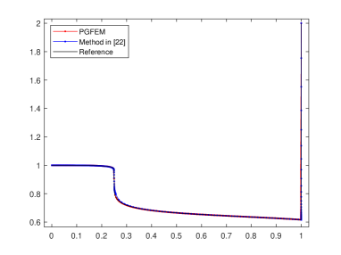
(a)

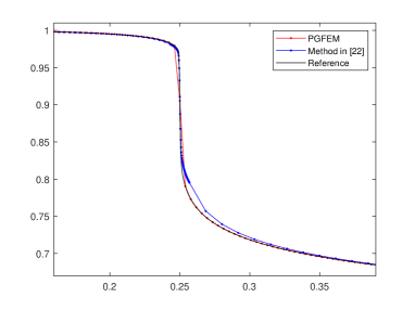
(b)

Figure 1: Numerical and reference solutions for Example 4.1 ($\varepsilon=1\times 10^{-6}$), where test functions in PGFEM are calculated with exact expressions. (a) PGFEM and the method in ²² are employed with grid number $N=256$, with the latter using an up-winding scheme on Shishkin mesh. The reference solution is computed with PGFEM on grids $N=4096$; (b) Horizontal Magnification near $x=1/4$.

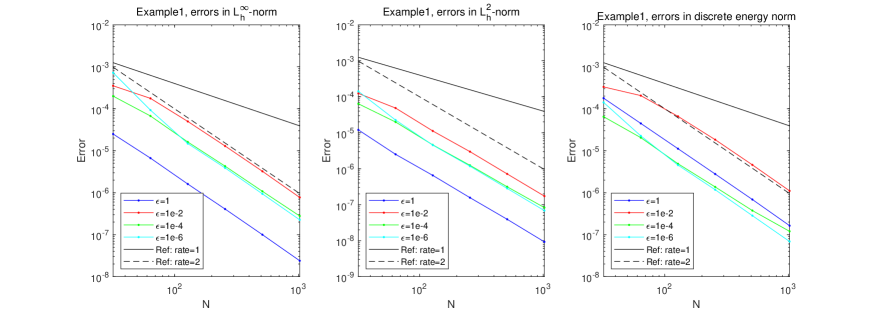
Figure 2: Log-log plot for PGFEM errors in Example 4.1 versus grid number $N$, in $L^{\infty}_{h},L^{2}_{h}$ and discrete energy norm. The solid black line and black dashed line have slopes -1 and -2, respectively.

Example 4.2.

Consider a boundary turning point problem:

$$\left\{\begin{aligned} &-\varepsilon u^{\prime\prime}+(1-x^{2})u^{\prime}+3u=e^{x},\quad-1<x<1,\\ &u(-1)=1,\quad u(1)=2.\\ \end{aligned}\right.$$

At both endpoints the solution appears singular with $p^{\prime}(-1)>0$ at $x=-1$ and $p^{\prime}(1)<0$ at $x=1$, corresponding to case (c) with a positive slope and a negative one. These two boundary layers are weaker than those in Example 4.1, as the PGFEM solution and the reference solution are drawn in Figure 3. Setting $\{-1,1\}$ as singular points and exact dual solutions as test functions, $L^{\infty}_{h}$ errors and discrete energy errors are shown in Tables 1 and 2 accordingly, where a first-order uniform convergence could be verified.

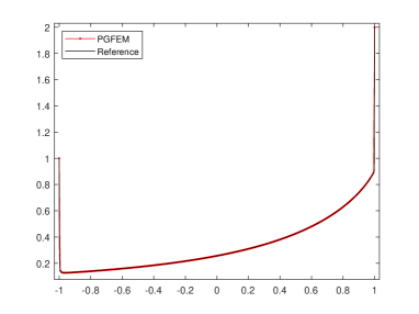
(a)

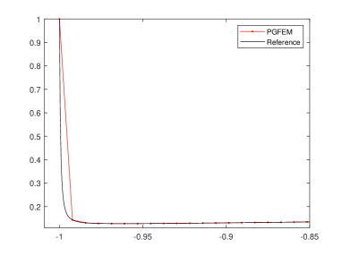
(b)

Figure 3: Numerical and reference solutions for Example 4.2 ($\varepsilon=1\times 10^{-6}$). Test functions in PGFEM are calculated with exact expressions. (a) PGFEM is implemented with grids $N=256$, and the reference solution is calculated using the same algorithm with $N=4096$; (b) Horizontal Magnification near $x=0$.

Table 1: $L^{\infty}_{h}$ errors of PGFEM solutions for Example 4.2. Test functions are calculated with exact expressions.

$\varepsilon$	1		1E-02		1E-04		1E-06
$N$	$L_{h}^{\infty}$	rate	$L_{h}^{\infty}$	rate	$L_{h}^{\infty}$	rate	$L_{h}^{\infty}$	rate
32	1.12E-04		2.78E-03		1.85E-03		1.85E-03
64	2.39E-05	2.43	1.46E-03	1.52	7.22E-04	2.10	7.16E-04	1.93
128	5.97E-06	2.00	3.72E-04	1.97	1.90E-04	1.93	1.83E-04	1.97
256	1.56E-06	1.98	7.86E-05	2.37	4.49E-05	2.26	8.66E-05	2.31
512	3.85E-07	2.02	1.94E-05	2.01	1.41E-05	1.89	3.73E-05	2.45
1024	9.07E-08	2.10	4.83E-06	2.04	3.33E-06	2.08	1.51E-05	2.22

Table 2: $||\cdot||_{\varepsilon,h}$ errors of PGFEM solutions for Example 4.2. Test functions are calculated with exact expressions.

$\varepsilon$	1		1.E-02		1.E-04		1.E-06
$N$	energy	rate	energy	rate	energy	rate	energy	rate
32	3.93E-04		1.95E-03		6.38E-04		6.27E-04
64	9.56E-05	2.24	9.93E-04	1.52	2.08E-04	1.84	2.09E-04	1.77
128	2.39E-05	2.00	2.55E-04	1.97	5.31E-05	1.99	5.50E-05	2.01
256	6.02E-06	2.03	5.47E-05	2.37	1.51E-05	2.17	1.42E-05	2.18
512	1.49E-06	2.02	1.35E-05	2.01	4.46E-06	2.01	3.93E-06	2.15
1024	3.53E-07	2.08	3.36E-06	2.05	1.24E-06	2.03	1.14E-06	2.13

For Example 4.2, if we compute test functions numerically, using the same reference solution, convergence is the same as above (see Table 3). Convergency also holds for multiple turning point problems if we follow the same procedure to compute test functions, although it is unclear what analytic expressions of the solutions to dual problems are.

Table 3: $L^{\infty}_{h}$ errors of PGFEM solutions for Example 4.2. Test functions are approximated by numerical solutions.

$\varepsilon$	1		1.E-02		1.E-04		1.E-06
$N$	$L_{h}^{\infty}$	rate	$L_{h}^{\infty}$	rate	$L_{h}^{\infty}$	rate	$L_{h}^{\infty}$	rate
32	1.12E-04		2.78E-03		1.86E-03		1.86E-03
64	2.39E-05	2.43	1.46E-03	1.52	7.23E-04	2.11	7.21E-04	1.94
128	5.96E-06	2.00	3.72E-04	1.97	1.90E-04	1.93	1.84E-04	1.97
256	1.56E-06	1.98	7.86E-05	2.37	4.50E-05	2.26	8.66E-05	2.32
512	3.85E-07	2.02	1.94E-05	2.01	1.40E-05	1.89	3.68E-05	2.45
1024	9.07E-08	2.10	4.83E-06	2.04	3.33E-06	2.08	1.51E-05	2.29

Example 4.3.

Consider the following multiple boundary turning point problem in³⁵:

$$\left\{\begin{aligned} &-\varepsilon u^{\prime\prime}-x^{3}u^{\prime}+u=f(x),\quad 0<x<1,\\ &u(0)=2,\quad u(1)=e^{-1/\sqrt{\varepsilon}}+e,\\ \end{aligned}\right.$$

where $f(x)$ is determined by the exact solution:

$$u(x)=e^{-x/\sqrt{\varepsilon}}+e^{x}.$$

There is a $\sqrt{\varepsilon}$-wide boundary layer at the turning point $x=0$, as drawn in Figure 4. Results of PGFEM are compared with one in ³⁵, where we compute with two methods on the same uniform mesh, and PGFEM obtains solutions with higher precision. In this case, analytic expressions of dual solutions are unknown. Thus we utilize numerical solutions to dual problems as test functions. The $L^{\infty}_{h}$ convergence rate of PGFEM is almost two, as shown in Table 4.

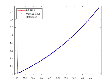
(a)

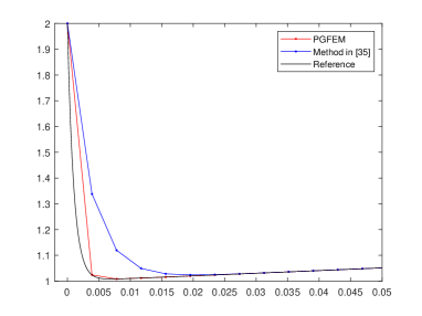
(b)

Figure 4: Numerical and exact solutions for Example 4.3 ($\varepsilon=1\times 10^{-6}$). Test functions in PGFEM are approximated by numerical solutions on grids $N=4096$. (a) PGFEM and the method in ³⁵ are manipulated with uniform grids $N=256$, and the reference solution is computed with PGFEM and $N=4096$; (b) Horizontal Magnification near $x=0$.

Table 4: $L^{\infty}_{h}$ errors of PGFEM solutions for Example 4.3. Test functions are approximated by numerical solutions.

$\varepsilon$	1		1.E-02		1.E-04		1.E-06
$N$	$L_{h}^{\infty}$	rate	$L_{h}^{\infty}$	rate	$L_{h}^{\infty}$	rate	$L_{h}^{\infty}$	rate
32	1.84E-05		1.65E-04		3.71E-04		1.05E-03
64	4.61E-06	2.00	4.82E-05	1.77	5.89E-05	2.66	3.01E-04	1.81
128	1.15E-06	2.00	1.26E-05	1.93	8.85E-06	2.82	7.64E-05	1.98
256	2.88E-07	2.00	3.20E-06	1.98	2.22E-06	1.99	1.77E-05	2.11
512	7.21E-08	2.00	8.02E-07	2.00	5.50E-07	2.01	4.57E-06	2.31
1024	1.79E-08	2.01	2.01E-07	2.00	1.33E-07	2.04	1.17E-06	1.97

5 Conclusion

In this paper, we develop a Petrov-Galerkin finite element method (PGFEM) to solve a class of turning point problems in one dimension. Priori estimates have been established for the single boundary turning point case. Numerical analysis shows that our scheme has first-order uniform convergency in several different norms. In numerical examples, errors in different discrete norms validate the feasibility and efficiency of the scheme. We emphasize that such an algorithm not only could be implemented with evaluations of exact solutions to the dual problems but also is considerable if test functions are approximated numerically.

References

- [1] Leif R Abrahamson. A priori estimates for solutions of singular perturbations with a turning point. Stud. Appl. Math., 56:1 (1977), 51–69.
- [2] Alan E Berger, Houde Han, and R Bruce Kellogg. A priori estimates and analysis of a numerical method for a turning point problem. Math. Comput., 42:166 (1984), 465–492.
- [3] Dirk Broersen and Rob Stevenson. A robust petrov–galerkin discretisation of convection–diffusion equations. Comput. Math. with Appl., 68:11 (2014), 1605–1618.
- [4] Ankit Chakraborty, Ajay Rangarajan, and Georg May. Optimal approximation spaces for discontinuous petrov-galerkin finite element methods. arXiv:2012.12751, (2020).
- [5] Long Chen, Yonggang Wang, and Jinbiao Wu. Stability of a streamline diffusion finite element method for turning point problems. J. Comput. Appl. Math., 220:1-2 (2008), 712–724.
- [6] Carlo De Falco and Eugene O’Riordan. A parameter robust Petrov–Galerkin scheme for advection–diffusion–reaction equations. Numer. Algorithms, 56:1 (2011), 107–127.
- [7] PPN De Groen and PW Hemker. Error bounds for exponentially fitted galerkin methods applied to stiff two-point boundary value problems, in London a.o : Academic Press, GBR, 1979, pp. 217–249.
- [8] TM El-Mistikawy and MJ Werle. Numerical method for boundary layers with blowing-the exponential box scheme. AIAA Journal, 16:7 (1978), 749–751.
- [9] Paul A Farrell. Sufficient conditions for the uniform convergence of a difference scheme for a singularly perturbed turning point problem. SIAM J. Numer. Anal., 25:3 (1988), 618–643.
- [10] Paul A Farrell and Eugene C Gartland Jr. A uniform convergence result for a turning point problem, in Proc. BAIL V Conference, China, 1988, pp. 127–132.
- [11] FZ Geng, SP Qian, and S Li. A numerical method for singularly perturbed turning point problems with an interior layer. J. Comput. Appl. Math., 255 (2014), 97–105.
- [12] Wen Guo. Uniformly convergent finite element methods for singularly perturbed parabolic partial differential equations. PhD thesis, University College Cork, 1993.
- [13] Houde Han and Zhongyi Huang. Tailored finite point method for steady-state reaction-diffusion equations. Commun. Math. Sci., 8:4 (2010), 887–899.
- [14] Houde Han and Zhongyi Huang. Tailored finite point method based on exponential bases for convection-diffusion-reaction equation. Math. Comput., 82:281 (2013), 213–226.
- [15] Houde Han, Zhongyi Huang, and R Bruce Kellogg. A tailored finite point method for a singular perturbation problem on an unbounded domain. J. Sci. Comput., 36:2 (2008), 243–261.
- [16] PW Hemker, GI Shishkin, and LP Shishkina. -uniform schemes with high-order time-accuracy for parabolic singular perturbation problems. IMA J. Numer. Anal., 20:1 (2000), 99–121.
- [17] Zhongyi Huang. Tailored finite point method for the interface problem. Netw. Heterog. Media, 4:1 (2009), 91–106.
- [18] R Bruce Kellogg and Alice Tsan. Analysis of some difference approximations for a singular perturbation problem without turning points. Math. Comput., 32:144 (1978), 1025–1039.
- [19] Devendra Kumar. A parameter-uniform method for singularly perturbed turning point problems exhibiting interior or twin boundary layers. Int. J. Comput. Math., 96:5 (2019), 865–882.
- [20] Jichun Li. Convergence analysis of finite element methods for singularly perturbed problems. Comput. Math. with Appl., 40:6-7 (2000), 735–745.
- [21] Justin B Munyakazi, Kailash C Patidar, and Mbani T Sayi. A robust fitted operator finite difference method for singularly perturbed problems whose solution has an interior layer. Math. Comput. Simul., 160 (2019), 155–167.
- [22] Srinivasan Natesan, J Jayakumar, and J Vigo-Aguiar. Parameter uniform numerical method for singularly perturbed turning point problems exhibiting boundary layers. J. Comput. Appl. Math., 158:1 (2003), 121–134.
- [23] Frank WJ Olver, Daniel W Lozier, Ronald F Boisvert, and Charles W Clark. NIST handbook of mathematical functions hardback and CD-ROM. Cambridge university press, 2010.
- [24] Eugene O’Riordan and Jason Quinn. A singularly perturbed convection diffusion turning point problem with an interior layer. Comput. Methods Appl. Math., 12:2 (2012), 206–220.
- [25] RE O’Malley, Jr. On boundary value problems for a singularly perturbed differential equation with a turning point. SIAM J. Math. Anal., 1:4 (1970), 479–490.
- [26] E O’Riordan and J Quinn. Parameter-uniform numerical methods for some linear and nonlinear singularly perturbed convection diffusion boundary turning point problems. BIT Numer. Math., 51:2 (2011), 317–337.
- [27] H-G Roos. Global uniformly convergent schemes for a singularly perturbed boundary-value problem using patched base spline-functions. J. Comput. Appl. Math., 29:1 (1990), 69–77.
- [28] Martin Stynes and Eugene O’Riordan. A finite element method for a singularly perturbed boundary value problem. Numer Math (Heidelb), 50:1 (1986), 1–15.
- [29] Martin Stynes and Eugene O’Riordan. and uniform convergence of a difference scheme for a semilinear singular perturbation problem. Numer Math (Heidelb), 50:5 (1987), 519–531.
- [30] Guangfu Sun and Martin Stynes. Finite element methods on piecewise equidistant meshes for interior turning point problems. Numer. Algorithms, 8:1 (1994), 111–129.
- [31] Guangfu Sun and Martin Stynes. Finite-element methods for singularly perturbed high-order elliptic two-point boundary value problems. i: reaction-diffusion-type problems. IMA J. Numer. Anal., 15:1 (1995), 117–139.
- [32] Nico M Temme. Numerical and asymptotic aspects of parabolic cylinder functions. J. Comput. Appl. Math., 121:1-2 (2000), 221–246.
- [33] Relja Vulanović. Non-equidistant generalizations of the Gushchin-Shchennikov scheme. Z. Angew. Math. Mech., 67:12 (1987), 625–632.
- [34] Relja Vulanović. On numerical solution of a mildly nonlinear turning point problem. Esaim Math. Model. Numer. Anal., 24:6 (1990), 765–783.
- [35] Relja Vulanović and Paul A Farrell. Continuous and numerical analysis of a multiple boundary turning point problem. SIAM J. Numer. Anal., 30:5 (1993), 1400–1418.
- [36] Swati Yadav and Pratima Rai. An almost second order hybrid scheme for the numerical solution of singularly perturbed parabolic turning point problem with interior layer. Math. Comput. Simul., 185 (2021), 733–753.