The Laplace operator, measure concentration,
Gauss functions, and quantum mechanics

Abstract

We represent in this note the solutions of the electronic Schrödinger equation as traces of higher-dimensional functions. This allows to decouple the electron-electron interaction potential but comes at the price of a degenerate elliptic operator replacing the Laplace operator on the higher-dimensional space. The surprising observation is that this operator can without much loss again be substituted by the Laplace operator, the more successful the larger the system under consideration is. This is due to a concentration of measure effect that has much to do with the random projection theorem known from probability theory. The text is in parts based on the publications [Numer. Math. 146, 219–238 (2020)] and [SIAM J. Matrix Anal. Appl., 43, 464–478 (2022)] of the author and adapts the findings there to the needs of quantum mechanics. Our observations could for example find use in iterative methods that map sums of products of orbitals and geminals onto functions of the same type.

1 Introduction

The electronic Schrödinger equation establishes a connection between chemistry and physics. It describes systems of electrons that interact among each other and with a given, fixed set of nuclei. The electronic Schrödinger equation motivated our former work Yserentant_2020 , Yserentant_2022 centered around the approximate solution of high-dimensional partial differential equations. The present text compiles some of these results in view of applications in quantum theory and adapts and complements them correspondingly. We think here, for example, of procedures like the approximate inverse iteration

$$u\;\,\leftarrow\;\,u\,-\,(-\Delta+\mu)^{-1}(-\Delta u+\mu u+Vu-\lambda(u)u)$$ (1)

for the calculation of the ground state energy or more general the first energy levels of a molecule, which requires the repeated (approximate) solution of the equation

$$-\Delta u+\mu u=f$$ (2)

on the $\mathbb{R}^{m}$ for high dimensions $m$, where $\mu>0$ is a given constant. Provided the right-hand side $f$ of the equation (2) possesses an integrable Fourier transform,

$$u(x)=\bigg{(}\frac{1}{\sqrt{2\pi}}\bigg{)}^{m}\!\int\frac{1}{\mu+\|\omega\|^{2}}\,\widehat{f}(\omega)\,\mathrm{e}^{\,\mathrm{i}\,\omega\cdot x}\,\mathrm{d}\omega$$ (3)

is a solution of this equation, and the only solution that tends uniformly to zero as x goes to infinity. If the right-hand side $f$ of the equation is a tensor product

$$f(x)=\prod_{i}\phi_{i}(x_{i})$$ (4)

of functions say from the three-dimensional space to the real numbers, or a sum of such tensor products, the same holds for the Fourier transform of $f$. If one replaces the corresponding term in the high-dimensional integral (3) by an approximation

$$\frac{1}{\mu+\|\omega\|^{2}}\approx\sum_{k}a_{k}\,\mathrm{e}^{-\beta_{k}\left(\mu+\|\omega\|^{2}\right)}=\sum_{k}a_{k}\,\mathrm{e}^{-\beta_{k}\mu}\prod_{i}\mathrm{e}^{-\beta_{k}\|\omega_{i}\|^{2}}$$ (5)

based on an approximation of $1/r$ by a sum of exponential functions, as described in Sect. 6, for example, the integral collapses in this case to a sum of products of lower-dimensional integrals. That is, the solution can, independent of the space dimension, be approximated by a sum of such tensor products. The right-hand sides involved in iterations like (1) are, however, not of such a simple structure. This is due to the fact that the potential $V$ is not only composed of terms depending on the position of a single electron in space, but also of terms that depend on the distance of two electrons. A corresponding ansatz for the solutions provided, this requires the solution of the equation (2) with right-hand sides that are composed of terms of the form

$$f(x)=\bigg{(}\prod_{i}\phi_{i}(x_{i})\bigg{)}\bigg{(}\prod_{i<j}\phi_{ij}(x_{i}-x_{j})\bigg{)}.$$ (6)

The question is whether this structure is reflected in the solution and the iterates stay in this class. To be precise, let us consider a system of $N$ electrons, let

$$m=3\times N,\quad n=3\times\frac{N(N+1)}{2},$$ (7)

and let the vectors in $\mathbb{R}^{m}$ and $\mathbb{R}^{n}$, respectively, be partitioned into subvectors in the position space $\mathbb{R}^{3}$. Let the subvectors of the vectors in $\mathbb{R}^{m}$ and the first $N$ of the subvectors of the vectors in $\mathbb{R}^{n}$ be labeled by the indices $i=1,\ldots,N$ and the remaining subvectors of the vectors in $\mathbb{R}^{n}$ by the index pairs $(i,j)$, $i,j=1,\ldots,N$ and $i<j$. Let the right-hand side of the equation (2) be of the form $f(x)=F(Tx)$, where $T$ maps the vectors $x\in\mathbb{R}^{m}$ into the vectors $Tx\in\mathbb{R}^{n}$ with the subvectors

$$Tx|_{i}=x_{i},\quad Tx|_{ij}=\frac{x_{i}-x_{j}}{\sqrt{2}},$$ (8)

and where $F$ is a correspondingly structured function from the higher-dimensional space $\mathbb{R}^{n}$ to $\mathbb{R}$. If this function possesses an integrable Fourier transform, the solution of the equation (2) is the trace $u(x)=U(Tx)$ of the function

$$U(y)=\bigg{(}\frac{1}{\sqrt{2\pi}}\bigg{)}^{n}\!\int\frac{1}{\mu+\|T^{t}\omega\|^{2}}\,\widehat{F}(\omega)\,\mathrm{e}^{\,\mathrm{i}\,\omega\cdot y}\,\mathrm{d}\omega$$ (9)

mapping the higher dimensional space to the real numbers. A in comparison to that in reference Yserentant_2020 considerably simplified, more direct proof of this proposition is given in Sect. 2. The key result of the present paper is that the function

$$\widetilde{U}(y)=\bigg{(}\frac{1}{\sqrt{2\pi}}\bigg{)}^{n}\!\int\frac{1}{\mu+\|\omega\|^{2}}\,\widehat{F}(\omega)\,\mathrm{e}^{\,\mathrm{i}\,\omega\cdot y}\,\mathrm{d}\omega,$$ (10)

that is, the solution of the equation $-\Delta U+\mu U=F$ on the higher-dimensional space, represents a with increasing particle number increasingly better and in the end almost perfect approximation of the function (9), so that we arrived again at the case of right-hand sides of the form (4). The reason is that the fraction of the vectors $\omega$ on the unit sphere for which the euclidean norm of $T^{t}\omega$ differs from one by more than a given small amount tends exponentially to zero as the number of electrons increases. This is a nontrivial concentration of measure phenomenon that has a lot to do with the random projection theorem (see Lemma 5.3.2 in Vershynin , for example), which plays an important role in the data sciences and is in close connection with the Johnson-Lindenstrauss theorem Johnson-Lindenstrauss . Section 3 of this text, which is in large parts more or less directly taken from Yserentant_2022 , is devoted to the study of this effect.

This observation can unsurprisingly be used in iterative methods for the solution of the Laplace-like equation (2), or, as indicated above, for the calculation of the ground state of a molecular system by some kind of approximate inverse iteration. A comprehensive theory of such methods (for the matrix case) is due to Knyazev and Neymeyr; see Knyazev-Neymeyr and the references cited therein, and Rohwedder-Schneider-Zeiser and Yserentant_2016 for the infinite dimensional case. But one can also speculate that this measure concentration effect allows to replace the original Schrödinger equation in case of sufficiently high particle numbers by a largely decoupled, higher-dimensional equation, with solutions whose traces become increasingly better approximations of the true wave functions.

2 Solutions as traces of higher-dimensional functions

We are in the following mainly concerned with functions $U:\mathbb{R}^{n}\to\mathbb{R}$, $n$ a potentially high dimension, that possess a then also unique representation

$$U(y)=\bigg{(}\frac{1}{\sqrt{2\pi}}\bigg{)}^{n}\!\int\widehat{U}(\omega)\,\mathrm{e}^{\,\mathrm{i}\,\omega\cdot y}\,\mathrm{d}\omega$$ (1)

in terms of an integrable function $\widehat{U}$, their Fourier transform. Such functions are by the Riemann-Lebesgue theorem uniformly continuous and vanish at infinity. The space $W_{0}(\mathbb{R}^{n})$ of these functions becomes under the norm

$$\|U\|=\bigg{(}\frac{1}{\sqrt{2\pi}}\bigg{)}^{n}\!\int|\widehat{U}(\omega)|\,\mathrm{d}\omega$$ (2)

a Banach space. Let $T$ be a still arbitrary $(n\times m)$-matrix of full rank $m<n$ and let

$$u:\mathbb{R}^{m}\to\mathbb{R}:x\to U(Tx)$$ (3)

be the trace of a function in $U\in W_{0}(\mathbb{R}^{n})$. As the functions in $W_{0}(\mathbb{R}^{n})$ are uniformly continuous, the same obviously holds for their traces. Because there is a constant $c$ with $\|x\|\leq c\,\|Tx\|$ for all $x\in\mathbb{R}^{m}$, the trace functions (3) vanish at infinity, too. The next lemma gives a criterion for the existence of partial derivatives of the trace functions, where we use the common multi-index notation.

Lemma 1

Let $U:\mathbb{R}^{n}\to\mathbb{R}$ be a function in $W_{0}(\mathbb{R}^{n})$ and let the functions

$$\omega\to(\mathrm{i}\,T^{t}\omega)^{\beta}\widehat{U}(\omega),\quad\beta\leq\alpha,$$ (4)

be integrable. The trace function (3) possesses then the partial derivative

$$(\mathrm{D}^{\alpha}u)(x)=\bigg{(}\frac{1}{\sqrt{2\pi}}\bigg{)}^{n}\!\int(\mathrm{i}\,T^{t}\omega)^{\alpha}\widehat{U}(\omega)\,\mathrm{e}^{\,\mathrm{i}\,\omega\cdot Tx}\,\mathrm{d}\omega,$$ (5)

which is like $u$ itself uniformly continuous and vanishes at infinity.

Proof

Let $e_{k}\in\mathbb{R}^{m}$ be the vector with the components $e_{k}|_{j}=\delta_{kj}$. To begin with, we examine the limit behavior of the difference quotient

$$\frac{u(x+he_{k})-u(x)}{h}=\bigg{(}\frac{1}{\sqrt{2\pi}}\bigg{)}^{n}\!\int\frac{\mathrm{e}^{\,\mathrm{i}\,h\omega\cdot Te_{k}}-1}{h}\;\widehat{U}(\omega)\,\mathrm{e}^{\,\mathrm{i}\,\omega\cdot Tx}\,\mathrm{d}\omega$$

of the trace function as $h$ goes to zero. If the function $\omega\to\omega\cdot Te_{k}\,\widehat{U}(\omega)$ is integrable, this difference quotient tends, because of

$$\bigg{|}\,\frac{\mathrm{e}^{\,\mathrm{i}\,ht}-1}{h}\,\bigg{|}\leq\,|\,t\,|,\quad\lim_{h\to 0}\frac{\mathrm{e}^{\,\mathrm{i}\,ht}-1}{h}=\,\mathrm{i}\,t,$$

by the dominated convergence theorem to the limit value

$$(\mathrm{D}_{k}u)(x)=\bigg{(}\frac{1}{\sqrt{2\pi}}\bigg{)}^{n}\!\int\mathrm{i}\,\omega\cdot Te_{k}\,\widehat{U}(\omega)\,\mathrm{e}^{\,\mathrm{i}\,\omega\cdot Tx}\,\mathrm{d}\omega.$$

Because of $\omega\cdot Te_{k}=T^{t}\omega\cdot e_{k}$, this proves (5) for partial derivatives of order one. For partial derivatives of higher order, the proposition follows by induction. ∎

Let $W_{0}^{2}(T)$ be the space of the functions $U\in W_{0}(\mathbb{R}^{n})$ with finite (semi)-norm

$$|\,U|_{T}=\bigg{(}\frac{1}{\sqrt{2\pi}}\bigg{)}^{n}\!\int\|T^{t}\omega\|^{2}\,|\widehat{U}(\omega)|\,\mathrm{d}\omega.$$ (6)

The traces of these functions are by Lemma 1 twice continuously differentiable. Let $\mathcal{L}:W_{0}^{2}(T)\to W_{0}(\mathbb{R}^{n})$ be the degenerate elliptic differential operator given by

$$(\mathcal{L}U)(y)=\bigg{(}\frac{1}{\sqrt{2\pi}}\bigg{)}^{n}\!\int\|T^{t}\omega\|^{2}\,\widehat{U}(\omega)\,\mathrm{e}^{\,\mathrm{i}\,\omega\cdot y}\,\mathrm{d}\omega.$$ (7)

For the functions $U\in W_{0}^{2}(T)$ and their traces (3), by Lemma 1

$$-\,(\Delta u)(x)=(\mathcal{L}U)(Tx)$$ (8)

holds. The solutions of the equation (2) thus are, with corresponding right-hand sides, the traces of the solutions $U\in W_{0}^{2}(T)$ of the differential equation

$$\mathcal{L}U+\mu U=F.$$ (9)

Theorem 2.1

Let $F:\mathbb{R}^{n}\to\mathbb{R}$ be a function with integrable Fourier transform, let $f(x)=F(Tx)$, and let $\mu$ be a positive constant. The trace (3) of the function

$$U(y)=\bigg{(}\frac{1}{\sqrt{2\pi}}\bigg{)}^{n}\!\int\frac{1}{\mu+\|T^{t}\omega\|^{2}}\,\widehat{F}(\omega)\,\mathrm{e}^{\,\mathrm{i}\,\omega\cdot y}\,\mathrm{d}\omega$$ (10)

is then twice continuously differentiable and the only solution of the equation

$$-\Delta u+\mu u=f$$ (11)

whose values tend uniformly to zero as $\|x\|$ goes to infinity.

That the trace $u$ is a classical solution of the equation (11) follows from the remarks above, and that $u$ vanishes at infinity from the Riemann-Lebesgue theorem. By the maximum principle from the next lemma, the trace $u$ is the only such solution.

Lemma 2

Let $u:\mathbb{R}^{m}\to\mathbb{R}$ be a twice continuously differentiable function that vanishes at infinity. Let $\mu>0$ and let $-\Delta u+\mu u\geq 0$. Then $u\geq 0$ everywhere.

Proof

Let $u(x_{0})<0$ at some point $x_{0}$ and let $|u(x)|<|u(x_{0})|$ for $\|x\|\geq R$. Then there exists a point $x_{1}$ of norm $\|x_{1}\|\leq R$ with $u(x_{1})\leq u(x)$ for all $x$ at first inside this ball. The function $u$ attains then at $x_{1}$ its global minimum. The Hessian of $u$ is at this point necessarily positive semidefinite, which implies that $\Delta u\geq 0$ there. Because $\mu>0$, at this point therefore $-\Delta u+\mu u<0$. This contradicts the assumption. ∎

As said, we are primarily interested in right-hand sides $F$ that themselves are products of lower-dimensional functions, or that are sums or rapidly converging series of such functions. It seems that the term

$$\frac{1}{\mu+\|T^{t}\omega\|^{2}}$$ (12)

destroys this structure and that the transition to the equation (9) is therefore of little value. In high dimensions, however, often the contrary holds due to the concentration of measure effects studied in the next section. For the matrix (8) assigned to the Schrödinger equation, the fraction of the vectors $\omega$ on the unit sphere of the $\mathbb{R}^{n}$ for which the euclidean norm of $T^{t}\omega$ differs from one by more than a given small amount tends exponentially to zero as the number of electrons goes to infinity. This means that we can replace the euclidean norm of $T^{t}\omega$ without much loss by that of $\omega$ itself and arrive again at the case described at the very beginning. If needed, the resulting approximations of the solutions of the equation (9) can be iteratively improved.

3 The underlying measure concentration effect

Let $n>m$ and let $A$ be a real $(m\times n)$-matrix of rank $m$. The kernel of such a matrix has the dimension $n-m$ and hence can, in dependence of the dimensions, be a large subspace of the $\mathbb{R}^{n}$. Nevertheless, the set of all $x$ for which

$$\|Ax\|\geq\delta\,\|A\|\|x\|$$ (1)

holds fills, in the high-dimensional case, often almost the complete $\mathbb{R}^{n}$ once $\delta$ falls below a certain bound; the norms are here and as in the previous section the euclidean norm on the $\mathbb{R}^{m}$ and the $\mathbb{R}^{n}$ and the assigned spectral norms of matrices. Let $\chi$ be the characteristic function of the set of all $x$ for which $\|Ax\|<\delta\,\|A\|\|x\|$ holds, and let $\nu_{n}$ be the volume of the unit ball in $\mathbb{R}^{n}$. The normed area measure

$$\frac{1}{n\nu_{n}}\int_{S^{n-1}}\!\chi(\eta)\,\mathrm{d}\eta$$ (2)

of the subset of the unit sphere on which the condition (1) is violated takes in such cases an extremely small value, which conversely again means that (1) holds on an overwhelmingly large part of the unit sphere and with that of the full space. We study this phenomenon in this section along the lines given in Yserentant_2022 for orthogonal projections, matrices of the given kind with one as the only singular value, and for a class of matrices that in a sense do not substantially differ from such projections and under which the transpose of the matrix $T$ described in the introduction falls.

The surface integrals (2) are not easily accessible and are difficult to calculate and estimate. We reformulate them therefore as volume integrals and draw some first conclusions from these representations. The starting point is the decomposition

$$\int_{\mathbb{R}^{n}}f(x)\,\mathrm{d}x\,=\int_{S^{n-1}}\bigg{(}\int_{0}^{\infty}\!f(r\eta)r^{n-1}\,\mathrm{d}r\bigg{)}\!\,\mathrm{d}\eta$$ (3)

of the integrals of functions in $L_{1}$ into an inner radial and an outer angular part. Inserting the characteristic function of the unit ball, one recognizes that the area of the $n$-dimensional unit sphere is $n\nu_{n}$, with $\nu_{n}$ the volume of the unit ball. If $f$ is rotationally symmetric, $f(r\eta)=f(re)$ holds for every $\eta\in S^{n-1}$ and every fixed, arbitrarily given unit vector $e$. In this case, (3) reduces therefore to

$$\int f(x)\,\mathrm{d}x\,=n\nu_{n}\int_{0}^{\infty}\!f(re)r^{n-1}\,\mathrm{d}r.$$ (4)

Lemma 3

Let $A$ be an arbitrary matrix of dimension $m\times n$, $m<n$, let $\chi$ be the characteristic function of the set of all $x\in\mathbb{R}^{n}$ for which $\|Ax\|<\delta\,\|A\|\|x\|$ holds, and let $W:\mathbb{R}^{n}\to\mathbb{R}$ be a rotationally symmetric weight function with integral

$$\int W(x)\,\mathrm{d}x\,=\,1.$$ (5)

The weighted surface integral (2) then takes the value

$$\int\chi(x)W(x)\,\mathrm{d}x.$$ (6)

Proof

Let $e$ be a given unit vector. For $\eta\in S^{n-1}$ and $r>0$ then $\chi(r\eta)=\chi(\eta)$ and $W(r\eta)=W(re)$ holds and the integral (6) can by (3) be written as

$$\int\chi(x)W(x)\,\mathrm{d}x\,=\int_{S^{n-1}}\chi(\eta)\bigg{(}\int_{0}^{\infty}\!W(re)r^{n-1}\,\mathrm{d}r\bigg{)}\!\,\mathrm{d}\eta.$$

Because the inner integral takes by (4) and (5) the value

$$\int_{0}^{\infty}\!W(re)r^{n-1}\,\mathrm{d}r=\frac{1}{n\nu_{n}},$$

this proves the proposition. ∎

An obvious choice for the weight function $W$ is the normed Gauss function

$$W(x)=\bigg{(}\frac{1}{\sqrt{\pi}}\bigg{)}^{n}\exp\big{(}-\|x\|^{2}\big{)}.$$ (7)

Another possible choice is the characteristic function of the unit ball $B$ of the $\mathbb{R}^{n}$ divided by its volume. For abbreviation, we introduce the probability measure

$$\lambda(M)=\frac{\mathrm{vol}(M\cap B)}{\mathrm{vol}(B)}$$ (8)

on the measurable subsets $M$ of the $\mathbb{R}^{n}$.

Lemma 4

Let $A$ be a matrix of dimension $m\times n$, $m<n$. The weighted integral (2) over the surface of the unit ball is then equal to the volume ratio

$$\lambda\big{(}\big{\{}x\,\big{|}\,\|Ax\|<\delta\,\|A\|\|x\|\big{\}}\big{)}.$$ (9)

Because the euclidean length of a vector and the volume of a set are invariant to orthogonal transformations, the surface ratio (2) and the volume ratio (9) as well depend only on the singular values of the matrix under consideration.

Lemma 5

Let $A$ be a matrix of dimension $m\times n$, $m<n$, with singular value decomposition $A=U\Sigma V^{t}$. The volume ratio (9) is then equal to the volume ratio

$$\lambda\big{(}\big{\{}x\,\big{|}\,\|\Sigma x\|<\delta\,\|\Sigma\|\|x\|\big{\}}\big{)},$$ (10)

that is, it depends exclusively on the singular values of the matrix $A$.

Proof

As the multiplication with the orthogonal matrices $U$ and $V^{t}$, respectively, does not change the euclidean norm of a vector, the set of all $x\in\mathbb{R}^{n}$ for which

$$\|Ax\|<\delta\,\|A\|\|x\|,\quad\|x\|\leq R,$$

holds coincides with the set of all $x$ for which we have

$$\|\Sigma V^{t}x\|<\delta\,\|\Sigma\|\|V^{t}x\|,\quad\|V^{t}x\|\leq R.$$

As the volume is invariant to orthogonal transformations, the proposition follows. ∎

Another simple and seemingly obvious observation is the following lemma.

Lemma 6

Let $A$ be a matrix of dimension $m\times n$, $m<n$, of full rank $m$. Then

$$\lim_{\delta\to 1-}\lambda\big{(}\big{\{}x\,\big{|}\,\|Ax\|<\delta\,\|A\|\|x\|\big{\}}\big{)}\,=\,1.$$ (11)

Proof

By Lemma 5, we can restrict ourselves to diagonal matrices $A=\Sigma$. Because the limit takes by the dominated convergence theorem the value

$$\lambda\big{(}\big{\{}x\,\big{|}\,\|\Sigma x\|<\|\Sigma\|\|x\|\big{\}}\big{)}$$

and since the set of all $x$ for which $\|\Sigma x\|=\|\Sigma\|\|x\|$ holds is as a lower-dimensional subspace of the $\mathbb{R}^{n}$ a set of measure zero, the proposition follows. ∎

For orthogonal projections, matrices $A$ with one as the only singular value, the volume ratios (9) possess a closed integral representation.

Theorem 3.1

Let the $(m\times n)$-matrix $P$ be an orthogonal projection. Then

$$\lambda\big{(}\big{\{}x\,\big{|}\,\|Px\|<\delta\,\|x\|\big{\}}\big{)}=F(\delta),\quad 0\leq\delta<1,$$ (12)

holds, where the function $F(\delta)=F(m,n;\delta)$ is defined by the integral expression

$$F(\delta)=\frac{2\,\Gamma(n/2)}{\Gamma(m/2)\Gamma((n-m)/2)}\,\int_{0}^{\delta}(1-t^{2})^{\alpha}t^{m-1}\,\mathrm{d}t$$ (13)

and the exponent $\alpha\geq-1/2$ is given by

$$\alpha=\frac{n-m-2}{2}.$$ (14)

It takes nonnegative values for dimensions $n\geq m+2$.

Proof

By Lemma 5, we can restrict ourselves to the matrix $P$ that extracts from a vector in $\mathbb{R}^{n}$ its first $m$ components. Consistent within the proof, we split the vectors in $\mathbb{R}^{n}$ into parts $x\in\mathbb{R}^{m}$ and $y\in\mathbb{R}^{n-m}$. The set whose volume has to be calculated consists then of the points in the unit ball for which

$$\|x\|<\delta\,\bigg{\|}\bigg{(}\,\begin{matrix}x\\ y\end{matrix}\,\bigg{)}\bigg{\|}$$

or, resolved for the norm of the component $x\in\mathbb{R}^{m}$,

$$\|x\|<\varepsilon\,\|y\|,\quad\varepsilon=\frac{\delta}{\sqrt{1-\delta^{2}}},$$

holds. The volume can then be expressed as double integral

$$\int\bigg{(}\int H\big{(}\varepsilon\|y\|-\|x\|\big{)}\chi\big{(}\|x\|^{2}+\|y\|^{2}\big{)}\,\mathrm{d}x\bigg{)}\,\mathrm{d}y,$$

where $H(t)=0$ for $t\leq 0$, $H(t)=1$ for $t>0$, $\chi(t)=1$ for $t\leq 1$, and $\chi(t)=0$ for arguments $t>1$. In terms of polar coordinates, that is, by (4), it reads as

$$(n-m)\nu_{n-m}\int_{0}^{\infty}\bigg{(}m\nu_{m}\int_{0}^{\varepsilon s}\chi\big{(}r^{2}+s^{2}\big{)}r^{m-1}\,\mathrm{d}r\bigg{)}s^{n-m-1}\,\mathrm{d}s,$$

with $\nu_{d}$ the volume of the $d$-dimensional unit ball. Substituting $t=r/s$ in the inner integral, the upper bound becomes independent of $s$ and the integral can be written as

$$(n-m)\nu_{n-m}\int_{0}^{\infty}\bigg{(}m\nu_{m}\,s^{m}\!\int_{0}^{\varepsilon}\chi\big{(}s^{2}(1+t^{2})\big{)}t^{m-1}\,\mathrm{d}t\bigg{)}s^{n-m-1}\,\mathrm{d}s.$$

Interchanging the order of integration, it attains the value

$$\frac{(n-m)\nu_{n-m}\,m\nu_{m}}{n}\int_{0}^{\varepsilon}\frac{t^{m-1}}{(1+t^{2})^{n/2}}\,\mathrm{d}t.$$

For abbreviation, we introduce the function

$$f(\delta)=g\bigg{(}\frac{\delta}{\sqrt{1-\delta^{2}}}\bigg{)},\quad g(\varepsilon)=\int_{0}^{\varepsilon}\frac{t^{m-1}}{(1+t^{2})^{n/2}}\,\mathrm{d}t,$$

on the interval $0\leq\delta<1$. With $\alpha$ given by (14), its derivative is

$$f^{\prime}(\delta)=(1-\delta^{2})^{\alpha}\delta^{m-1}.$$

Because $f(0)=0$, it possesses therefore the representation

$$f(\delta)=\int_{0}^{\delta}(1-t^{2})^{\alpha}t^{m-1}\,\mathrm{d}t.$$

Dividing the expression above by $\nu_{n}$ and remembering that

$$\nu_{d}=\frac{2}{d}\,\frac{\pi^{d/2}}{\Gamma(d/2)},$$

this completes the proof of the theorem. ∎

If the difference of the dimensions is even, the function (13) is an either even or odd polynomial of degree $n-2$ in $\delta$. A closed representation is given in Yserentant_2022 . For practical purposes, it is more advantageous to calculate $F(\delta)$ numerically by means of a quadrature rule. By (11), $F$ takes the value $F(1)=1$. Thus $F(\delta)=F(\delta)/F(1)$, so that there is no need to evaluate the Gamma function.

The function (13) always represents a lower bound for the volume ratios (9), independent of particular properties of the matrix under consideration.

Theorem 3.2

Let $A$ be a nonvanishing matrix of dimension $m\times n$, $m<n$. Then

$$\lambda\big{(}\big{\{}x\,\big{|}\,\|Ax\|<\delta\,\|A\|\|x\|\big{\}}\big{)}\,\geq\,F(m,n;\delta).$$ (15)

Proof

We can restrict ourselves to diagonal matrices $A=\Sigma$. Let $P$ be the matrix that extracts from a vector in $\mathbb{R}^{n}$ the first $m$ components. As $\|\Sigma x\|\leq\|\Sigma\|\|Px\|$ and $\|\Sigma\|>0$, the given volume ratio is then bounded from below by the volume ratio

$$\lambda\big{(}\big{\{}x\,\big{|}\,\|Px\|<\delta\,\|x\|\big{\}}\big{)}.$$

The proposition thus follows from Theorem 3.1. ∎

Upper bounds for the volume ratio (9) depend in general on the singular values of the matrix, in the extreme case on its condition number, the ratio of its maximum and its minimum singular value Yserentant_2022 . This is fortunately not the case for the matrices $A=T^{t}$, with $T$ given by (8), in which we are interested here and to which the next theorem applies. The euclidean norm of the vector $Tx\in\mathbb{R}^{n}$ is given by

$$\|Tx\|^{2}=\,\sum_{i=1}^{N}\|x_{i}\|^{2}+\,\frac{1}{4}\,\sum_{i=1}^{N}\sum_{j=1}^{N}\|x_{i}-x_{j}\|^{2}$$ (16)

or, after rearrangement, with the rank three map $T_{0}x=x_{1}+x_{2}+\cdots+x_{N}$ by

$$\|Tx\|^{2}=\,\frac{N+2}{2}\,\|x\|^{2}-\,\frac{1}{2}\,\|T_{0}x\|^{2}.$$ (17)

The $(m\times m)$-matrix $T^{t}T$ thus has the eigenvalue $(N+2)/2$ of multiplicity $m-3$ and the eigenvalue $1$ of multiplicity $3$. The singular values of the matrix $T^{t}$ are therefore

$$\sigma_{i}=1\;\text{for $\,i\leq 3$},\quad\sigma_{i}=\sqrt{\frac{N+2}{2}}\;\,\text{for $\,i\geq 4$}.$$ (18)

The spectral norm of the matrix $T^{t}$ is $\sqrt{(N+2)/2}$.

Theorem 3.3

Let $n>m$ and let $A$ be a nonvanishing $(m\times n)$-matrix with singular values $\sigma_{k}=\sigma_{m}$ for $k>m_{0}$. The volume ratio (9) satisfies then the estimate

$$\lambda\big{(}\big{\{}x\,\big{|}\,\|Ax\|<\delta\,\|A\|\|x\|\big{\}}\big{)}\leq F(m-m_{0},n;\delta).$$ (19)

Proof

We can restrict ourselves to diagonal matrices $A=\Sigma$. Let $P^{\prime}$ be the matrix that extracts from a vector $x\in\mathbb{R}^{n}$ its components $x_{k}$, $m_{0}<k\leq m$. As $\|\Sigma\|\|P^{\prime}x\|\leq\|\Sigma x\|$ and $\|\Sigma\|>0$, the volume ratio (19) is then less than or equal to the volume ratio

$$\lambda\big{(}\big{\{}x\,\big{|}\,\|P^{\prime}x\|<\delta\,\|x\|\big{\}}\big{)}.$$

The proposition follows again from its representation in Theorem 3.1. ∎

Next, we study the limit behavior of the function (13) when the dimensions tend to infinity. The subsequent estimates are expressed in terms of the function

$$\phi(\vartheta)=\vartheta\,\exp\bigg{(}\frac{1-\vartheta^{2}}{2}\bigg{)}.$$ (20)

It increases on the interval $0\leq\vartheta\leq 1$ strictly, attains at the point $\vartheta=1$ its maximum value one, and decreases from there again strictly.

Theorem 3.4

Let $\xi$ be the square root of the dimension ratio $m/n$. For $\delta<\xi$, then

$$0\,\leq\,F(m,n;\delta)\leq\,\phi\bigg{(}\frac{\delta}{\xi}\bigg{)}^{m}.$$ (21)

Proof

Let $P$ be the matrix that extracts from a vector in $\mathbb{R}^{n}$ its first $m$ components. The characteristic function $\chi$ of the set of all $x$ for which $\|Px\|<\delta\,\|x\|$ holds satisfies, for any $t>0$, the crucial, even if obviously not very sharp estimate

$$\chi(x)<\exp\big{(}\,t\,\big{(}\delta^{2}\|x\|^{2}-\|Px\|^{2}\big{)}\big{)}$$

by a product of univariate functions. By Lemma 3 and the subsequent remark, the volume ratio (12) can therefore be estimated by the integral

$$\bigg{(}\frac{1}{\sqrt{\pi}}\bigg{)}^{n}\!\int\exp\big{(}\,t\,\big{(}\delta^{2}\|x\|^{2}-\|Px\|^{2}\big{)}\big{)}\exp\big{(}-\|x\|^{2}\big{)}\,\mathrm{d}x$$

that remains finite for all $t$ in the interval $0\leq t<1/\delta^{2}$. It splits into a product of one-dimensional integrals and takes, for given $t$, the value

$$\bigg{(}\frac{1}{1-\delta^{2}t+t}\bigg{)}^{m/2}\bigg{(}\frac{1}{1-\delta^{2}t}\bigg{)}^{(n-m)/2}.$$

This expression attains its minimum on the interval $0<t<1/\delta^{2}$ at

$$t=\frac{\xi^{2}-\delta^{2}}{(1-\delta^{2})\delta^{2}}$$

and takes at this point $t$ the value

$$\bigg{(}\,\frac{\delta}{\xi}\,\bigg{(}\frac{1-\delta^{2}}{1-\xi^{2}}\bigg{)}^{\gamma}\;\bigg{)}^{m},\quad\gamma=\frac{1-\xi^{2}}{2\xi^{2}}.$$

If one sets $\delta/\xi=\vartheta$ for abbreviation, the logarithm

$$\ln\bigg{(}\bigg{(}\frac{1-\delta^{2}}{1-\xi^{2}}\bigg{)}^{\gamma}\;\bigg{)}=\,\frac{1-\xi^{2}}{2\xi^{2}}\,\ln\bigg{(}\frac{1-\vartheta^{2}\xi^{2}}{1-\xi^{2}}\bigg{)}$$

possesses, because of $\vartheta^{2}\xi^{2}<1$ and $\xi^{2}<1$, the power series expansion

$$\frac{1-\vartheta^{2}}{2}-\frac{1}{2}\,\sum_{k=1}^{\infty}\bigg{(}\frac{1-\vartheta^{2k}}{k}-\,\frac{1-\vartheta^{2k+2}}{k+1}\bigg{)}\xi^{2k}.$$

Because the series coefficients are for all $\vartheta\geq 0$ greater than or equal to zero and, by the way, polynomial multiples of $(1-\vartheta^{2})^{2}$, the proposition follows. ∎

Theorem 3.4 possesses a counterpart that deals with values $\delta$ greater than the square root of the ratio of the dimensions $m$ and $n$.

Theorem 3.5

Let $\xi$ be the square root of the dimension ratio $m/n$. For $\delta>\xi$, then

$$0\,\leq\,1-F(m,n;\delta)\leq\,\phi\bigg{(}\frac{\delta}{\xi}\bigg{)}^{m}.$$ (22)

Proof

The proof almost coincides with that of the previous theorem. Let $P$ be again the matrix that extracts from a vector in $\mathbb{R}^{n}$ its first $m$ components. Instead of the volume ratio (12), now we have to estimate the volume ratio

$$1-\lambda\big{(}\big{\{}x\,\big{|}\,\|Px\|<\delta\,\|x\|\big{\}}\big{)}=\lambda\big{(}\big{\{}x\,\big{|}\,\|Px\|\geq\delta\,\|x\|\big{\}}\big{)}.$$

For sufficiently small positive values $t$, it can be estimated by the integral

$$\bigg{(}\frac{1}{\sqrt{\pi}}\bigg{)}^{n}\!\int\exp\big{(}\,t\,\big{(}\|Px\|^{2}-\delta^{2}\|x\|^{2}\big{)}\big{)}\exp\big{(}-\|x\|^{2}\big{)}\,\mathrm{d}x.$$

This integral splits into a product of one-dimensional integrals and takes the value

$$\bigg{(}\frac{1}{1+\delta^{2}t-t}\bigg{)}^{m/2}\bigg{(}\frac{1}{1+\delta^{2}t}\bigg{)}^{(n-m)/2},$$

which attains, for $\delta<1$, on the interval $0<t<1/(1-\delta^{2})$ its minimum at

$$t=\frac{\delta^{2}-\xi^{2}}{(1-\delta^{2})\delta^{2}}.$$

It takes at this point $t$ again the value

$$\bigg{(}\,\frac{\delta}{\xi}\,\bigg{(}\frac{1-\delta^{2}}{1-\xi^{2}}\bigg{)}^{\gamma}\;\bigg{)}^{m},\quad\gamma=\frac{1-\xi^{2}}{2\xi^{2}}.$$

This leads as in the proof of Theorem 3.4 to the estimate (22). ∎

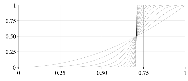
Figure 1: The volume ratio (12) as function of $0\leq\delta<1$ for $m=2^{k}$, $k=1,\ldots,16$, and $n=2m$

If the dimension ratio $\delta_{0}^{2}=m/n$ is kept fixed or only tends to $\delta_{0}^{2}$, the volume ratios (12) and the functions (13), respectively, thus tend to a step function with jump discontinuity at $\delta_{0}$. Figure 1 reflects this behavior. We summarize our findings therefore once more as follows and relate them to the prospective jump positions.

Theorem 3.6

Let $A$ be a nonvanishing matrix of dimension $m\times n$, $m<n$, and let $\xi$ be the square root of the dimension ratio $m/n$. For $\vartheta>1$ then one has

$$\lambda\big{(}\big{\{}x\,\big{|}\,\|Ax\|\geq\vartheta\xi\|A\|\|x\|\big{\}}\big{)}\leq\phi(\vartheta)^{m}.$$ (23)

Proof

As the set of the $x$ for which $\|Ax\|\geq\|A\|\|x\|$ holds is as a lower-dimensional subspace of the $\mathbb{R}^{n}$ a set of measure zero, we can restrict ourselves to the case $\vartheta\xi<1$. Setting $\delta=\vartheta\xi$, the proposition then follows from Theorem 3.2 and Theorem 3.5. ∎

The theorem states in particular that the norm of $Ax$ exceeds the value $\xi\|A\|\|x\|$ by more than a moderate factor $\vartheta>1$ only on a very small, de facto negligibly sector, an observation that is of great importance for the analysis of iterative methods for the solution of equations like (9). Under the much more restrictive assumptions from Theorem 3.3, Theorem 3.6 possesses a counterpart for values $\vartheta<1$.

Theorem 3.7

Let $n>m$ and let $A$ be a nonvanishing $(m\times n)$-matrix with singular values $\sigma_{k}=\sigma_{m}$ for $k>m_{0}$. If $m^{\prime}=m-m_{0}$ and $\xi^{\prime}$ is the square root of $m^{\prime}/n$, then

$$\lambda\big{(}\big{\{}x\,\big{|}\,\|Ax\|<\vartheta\xi^{\prime}\|A\|\|x\|\big{\}}\big{)}\leq\phi(\vartheta)^{m^{\prime}}$$ (24)

holds for all $\vartheta$ in the interval $0<\vartheta<1$.

Proof

This results from the estimates in Theorem 3.3 and Theorem 3.4. ∎

4 Back to the equation

The last two theorems apply, because of (18), to the matrices $A=T^{t}$ assigned to the Schrödinger equation. They form the basis of our argumentation. For a randomly chosen vector $\omega$ in the frequency or momentum space, the probability that

$$(1-\varepsilon)\xi^{\prime}\,\|T^{t}\|\|\omega\|\leq\|T^{t}\omega\|<(1+\varepsilon)\xi\,\|T^{t}\|\|\omega\|$$ (1)

holds for a given $\varepsilon$ between $0$ and $1$ is by these theorems at least

$$1-\big{(}\phi(1-\varepsilon)^{m^{\prime}}+\phi(1+\varepsilon)^{m}\big{)},$$ (2)

where $\phi$ is the function (20), the dimensions

$$m=3\times N,\quad n=3\times\frac{N(N+1)}{2},$$ (3)

and $m^{\prime}=3\times(N-1)$ depend on the number $N$ of particles, $\xi$ and $\xi^{\prime}$ are the square roots of the dimension ratios $m/n$ and $m^{\prime}/n$, and the constants

$$\xi^{\prime}\,\|T^{t}\|=\sqrt{1-\frac{2}{N(N+1)}},\quad\xi\,\|T^{t}\|=\sqrt{\vphantom{1-\frac{2}{N(N+1)}}1+\frac{1}{N+1}}$$ (4)

enclose the value one and tend to one as $N$ goes to infinity. The norm of $T^{t}\omega$ thus rapidly approaches that of $\omega$ when the number of particles increases. Because of

$$\phi(1\pm\varepsilon)<\exp(-c\,\varepsilon^{2}),\quad c=-\ln(\phi(2)),$$ (5)

for values $0<\varepsilon<1$, the probability that (1) holds is in any case greater than

$$1-2\exp(-c\,\varepsilon^{2}m^{\prime}).$$ (6)

A less easily interpretable, but significantly better lower bound than (2) can be derived from Theorem 3.2 and Theorem 3.3. In terms of the function (13), it reads

$$F(m,n;(1+\varepsilon)\xi)-F(m^{\prime},n;(1-\varepsilon)\xi^{\prime})$$ (7)

and deviates for increasing particle number less and less from the probability

$$F(m,n;(1+\varepsilon)\xi)-F(m,n;(1-\varepsilon)\xi)$$ (8)

that an orthogonal projection from the $\mathbb{R}^{n}$ to the $\mathbb{R}^{m}$ maps a randomly chosen unit vector to a vector of length between $(1-\varepsilon)\xi$ and $(1+\varepsilon)\xi$. Because the products of the matrix $T^{t}$ with vectors $e=e_{i}$ and $e=e_{ij}$ in $\mathbb{R}^{n}$ pointing into the direction of the coordinate spaces have the norm $\|T^{t}e\|=\|e\|$, they satisfy the condition

$$\xi^{\prime}\,\|T^{t}\|\|e\|<\|T^{t}e\|<\xi\,\|T^{t}\|\|e\|.$$ (9)

This establishes a link to hyperbolic cross spaces and not least to the mixed regularity of electronic wave functions Yserentant_2010 , Yserentant_2011 .

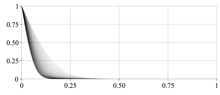
Figure 2: The distance of the lower bound (7) to one as function of $\varepsilon$ for $N=8,\ldots,64$ electrons.

What does all this mean? For high electron numbers, at the latest when statistical physics comes into play, the norm of $T^{t}\omega$ is almost equal to that of $\omega$ for all $\omega$ outside of a tiny, probably largely negligible sector. Maybe that this allows to replace the operator (7) in such cases by the negative Laplace operator and the original Hamilton operator to some extent by a correspondingly decoupled operator. But also for moderate particle numbers, the function (10),

$$\widetilde{U}(y)=\bigg{(}\frac{1}{\sqrt{2\pi}}\bigg{)}^{n}\!\int\frac{1}{\mu+\|\omega\|^{2}}\,\widehat{F}(\omega)\,\mathrm{e}^{\,\mathrm{i}\,\omega\cdot y}\,\mathrm{d}\omega,$$ (10)

that is, the solution of the equation $-\Delta U+\mu U=F$ in the higher-dimensional space, remains a good approximation to the solution (10) of the equation (9), surely good enough to serve as a building block for the construction of rapidly convergent iterative methods. Figure 2 shows the distance of the bound (7) to one as function of $\varepsilon$ for some small to medium size systems.

5 Square integrable right-hand sides

The fact that the function (10) is a good approximation of the solution (10) of the equation (9) depends in no way on the integrability of the Fourier transform of the right-hand side. The problem is that, for functions in the majority of $L_{2}$-based spaces, the transition to the trace functions is much more delicate than for the functions with integrable Fourier transforms. To a certain extent, smoothing of the right-hand side helps and mitigates this problem. Let $K:\mathbb{R}^{n}\to\mathbb{R}$ be a both integrable and square integrable normed kernel, like one of those with the Fourier transforms

$$\widehat{K}(\omega)=\bigg{(}\frac{1}{\sqrt{2\pi}}\bigg{)}^{n}\prod_{i=1}^{n}\phi\bigg{(}\frac{\omega_{i}^{2}}{2}\bigg{)},\quad\phi(t)=\mathrm{e}^{-t}\sum_{k=0}^{\nu}\frac{t^{k}}{k!},$$ (1)

depicted in Fig. 3 and with vanishing moments up to order $2\nu+1$, and let

$$K_{\varepsilon}(x)=\frac{1}{\varepsilon^{n}}\,K\Big{(}\frac{x}{\varepsilon}\Big{)}.$$ (2)

The convolution $K_{\varepsilon}*F$ both of square integrable functions $F$ and of functions $F$ with integrable Fourier transform possesses then the Fourier transform

$$(\widehat{K_{\varepsilon}*F})(\omega)=(\sqrt{2\pi})^{n}\widehat{K}(\varepsilon\omega)\widehat{F}(\omega),$$ (3)

which is in both cases integrable. For functions $F$ with integrable Fourier transform, this follows from the boundedness of $\widehat{K}$, and for square integrable functions $F$, it follows from the Cauchy-Schwarz inequality and Plancherel’s theorem.

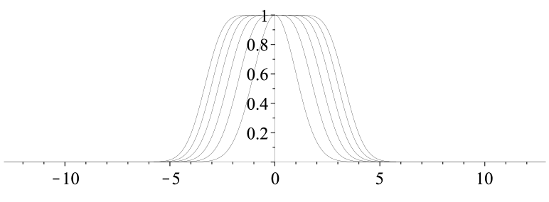
Figure 3: The renormalized Fourier transforms (1) in one space dimension for $\nu=0,1,\ldots,5$

The transition from the right-hand side $F$ to its smoothed variant $K_{\varepsilon}*F$ means that the solution $U$ of the equation (9) is replaced by its smoothed counterpart $K_{\varepsilon}*U$. If the Fourier transform of $F$ is integrable, not much gets lost. The reason is that the maximum norm of functions in $W_{0}(\mathbb{R}^{n})$ can be estimated by the scaled $L_{1}$-norm (2) of their Fourier transforms. As $\varepsilon$ goes to zero, the functions $K_{\varepsilon}*U$ converge therefore uniformly to $U$ and their traces $u_{\varepsilon}$ uniformly to the trace $u$ of $U$. Because of their representation from Lemma 1, the first- and second order derivatives of the $u_{\varepsilon}$ converge in the same way uniformly to the corresponding derivatives of $u$. For square integrable right-hand sides $F$, the situation is considerably more complicated. Only if the traces of the functions $K_{\varepsilon}*F$ tend in the $L_{2}$-sense to a limit function $f$, the $u_{\varepsilon}$ tend in the Sobolev space $H^{2}$ to a solution $u$ of the equation (11).

6 The approximation by exponential functions

We still need to approximate $1/r$ on given intervals $\mu\leq r\leq R\mu$ with moderate to high relative accuracy by sums of exponential functions. It suffices to restrict oneself to the case $\mu=1$, that is, to intervals $1\leq r\leq R$. If $v(r)$ approximates $1/r$ on this interval with a given relative accuracy, the rescaled function

$$r\;\to\;\frac{1}{\mu}\,v\bigg{(}\frac{r}{\mu}\bigg{)}$$ (1)

approximates $1/r$ on the interval $\mu\leq r\leq R\mu$ with the same relative accuracy. Our favorite approximations of $1/r$ are the at first sight harmless looking sums

$$v(r)=h\sum_{k=k_{1}}^{k_{2}}\mathrm{e}^{-kh}\exp(-\mathrm{e}^{-kh}r),$$ (2)

a construction that is due to Beylkin and Monzón Beylkin-Monzon . The parameter $h$ determines the accuracy and the quantities $k_{1}h$ and $k_{2}h$ control the approximation interval. The functions (2) possess the representation

$$v(r)=\frac{\phi(\ln r)}{r},\quad\phi(s)=\,h\sum_{k=k_{1}}^{k_{2}}\varphi(s-kh),$$ (3)

in terms of the for $s$ going to infinity rapidly decaying window function

$$\varphi(s)=\exp(-\mathrm{e}^{s}+s).$$ (4)

To check with which relative error the function (2) approximates $1/r$ on a given interval $1\leq r\leq R$, thus one has to examine how well the function $\phi$ approximates the constant $1$ on the interval $0\leq s\leq\ln R$. The functions (2) decay exponentially as $r$ goes to infinity. This means in the given context that high frequencies in the Fourier representation of the functions under consideration are already inherently more or less strongly damped, without the need for additional measures.

For $h=1$ and summation indices ranging from $k_{1}=-2$ to $k_{2}=50$, the relative error is, for instance, less than $0.0007$ on almost the whole interval $\mu\leq r\leq 10^{18}\mu$, that is, in the per mill range on an interval that spans eighteen orders of magnitude. Figure 3 shows the corresponding function $\phi$. The good approximation properties of the functions (2) are underpinned by the analysis in (Scholz-Yserentant, , Sect. 5) of the approximation properties of the corresponding infinite series. It has been shown there that these series approximate $1/r$ with a relative error

$$\sim 4\pi h^{-1/2}\mathrm{e}^{-\pi^{2}/h}$$ (5)

as $h$ goes to zero, that is, already for surprisingly large $h$ with very high accuracy. Approximations of similar kind, which try to minimize the absolute instead of the relative error, have been studied by Braess and Hackbusch Braess-Hackbusch , Braess-Hackbusch_2 .

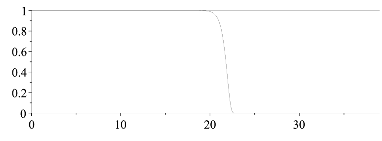
Figure 4: The rescaled function $s\to\phi(s\ln 10)$ approximating $1$ for $h=1$, $k_{1}=-2$, and $k_{2}=50$.

7 Symmetry properties of the solution and of its approximations

Electronic wave functions are subject to the Pauli principle. Taking spin into account, they are antisymmetric with respect to the exchange of the electrons, and if one considers the different spin components of the wave functions separately, antisymmetric with respect to the exchange of the positions of the electrons with the same spin. The aim of this section is to show that the given approximations do not lead out of classes of functions with corresponding symmetry properties.

To every permutation $\pi$ of the electron indices $1,\ldots,N$, we assign two orthogonal matrices, first the $(m\times m)$-permutation matrix $P$ given by

$$Px|_{i}=x_{\pi(i)},\quad i=1,\ldots,N,$$ (1)

and then the much larger orthogonal $(n\times n)$-matrix $Q$ given by

$$Qy|_{i}=y_{\pi(i)}$$ (2)

for the first $N$ subvectors $Qy|_{i}\in\mathbb{R}^{3}$ of $Qy$ and by

$$Qy|_{ij}=\begin{cases}\;y_{\pi(i),\pi(j)},&\text{if $\pi(i)<\pi(j)$}\\ -y_{\pi(j),\pi(i)},&\text{otherwise}\end{cases}$$ (3)

for the remaining subvectors in $\mathbb{R}^{3}$ that are, as described in the introduction, labeled by the index pairs $(i,j)$, $i,j=1,\ldots,N$, $i<j$. Moreover, we assign to $Q$ the value

$$\epsilon(Q)=\mathrm{sign}(\pi),$$ (4)

that is, the number $\epsilon(Q)=+1$, if $\pi$ is composed of an even number of transpositions, and the number $\epsilon(Q)=-1$ otherwise. By the definition (8) of the matrix $T$, then

$$TP=QT$$ (5)

holds. Let $G$ be a subgroup of the symmetric group $S_{N}$, the group of the permutations of the indices $1,\ldots,N$. The matrices assigned to the elements of $G$ form then, with the matrix multiplication as composition, groups that are isomorphic to $G$. We say that a function $u:\mathbb{R}^{m}\to\mathbb{R}$ is antisymmetric under the permutations in $G$, or shortly antisymmetric under $G$, if for all matrices $P=P(\pi)$ assigned to the $\pi\in G$

$$u(Px)=\mathrm{sign}(\pi)u(x)$$ (6)

holds. We say that a function $U:\mathbb{R}^{n}\to\mathbb{R}$ is antisymmetric under $G$ if for all these permutations $\pi$ and the assigned matrices $Q=Q(\pi)$

$$U(Qy)=\epsilon(Q)U(y)$$ (7)

holds. Both properties correspond to each other.

Lemma 7

If the function $U:\mathbb{R}^{n}\to\mathbb{R}$ is antisymmetric under $G$, so are its traces.

Proof

This follows by construction. By (5) we have

$$U(TPx)=U(QTx)=\epsilon(Q)U(Tx).$$

Because of $\epsilon(Q)=\mathrm{sign}(\pi)$, the proposition follows. ∎

We say that a function $U:\mathbb{R}^{n}\to\mathbb{R}$ is symmetric under the permutations in $G$, or shortly symmetric under $G$, if for all matrices $Q=Q(\pi)$, $\pi\in G$,

$$U(Qy)=U(y)$$ (8)

holds. Since the matrices $Q(\pi)$ assigned to the permutations in $\pi\in G$ are orthogonal, rotationally symmetric functions have this property.

We show in the following that, for any right-hand side $F$ of the equation (9) that is antisymmetric under the permutations in $G$, also its solution (10) is antisymmetric under $G$ and that the same holds for the described approximations of this solution.

Lemma 8

If the function $F\in W_{0}(\mathbb{R}^{n})$ is antisymmetric under $G$, so are, for any measurable and bounded kernel $K$ that is symmetric under $G$, also the functions

$$U(y)=\bigg{(}\frac{1}{\sqrt{2\pi}}\bigg{)}^{n}\!\int K(\omega)\,\widehat{F}(\omega)\,\mathrm{e}^{\,\mathrm{i}\,\omega\cdot y}\,\mathrm{d}\omega$$ (9)

antisymmetric under the permutations in $G$.

Proof

From the orthogonality of $Q$, we obtain

$$U(Qy)=\bigg{(}\frac{1}{\sqrt{2\pi}}\bigg{)}^{n}\!\int K(Q\omega)\,\widehat{F}(Q\omega)\,\mathrm{e}^{\,\mathrm{i}\,\omega\cdot y}\,\mathrm{d}\omega$$

and in the same way the representation

$$\widehat{F}(Q\omega)=\bigg{(}\frac{1}{\sqrt{2\pi}}\bigg{)}^{n}\!\int F(Qy)\,\mathrm{e}^{\,-\mathrm{i}\,\omega\cdot y}\,\mathrm{d}y.$$

Because of $F(Qy)=\epsilon(Q)F(y)$, the Fourier transform of $F$ thus transforms like

$$\widehat{F}(Q\omega)=\epsilon(Q)\widehat{F}(\omega).$$

As by assumption $K(Q\omega)=K(\omega)$, the proposition follows. ∎

The norm $\|\omega\|$ of the vectors $\omega$ in $\mathbb{R}^{n}$ is symmetric under the permutations in $G$, but also the norm of the vectors $T^{t}\omega$ in $\mathbb{R}^{m}$. This follows from the interplay of the matrices $P$, $Q$, and $T$, which finds expression in the relation (5) and leads to

$$\|T^{t}Q\omega\|=\|P^{t}T^{t}Q\omega\|=\|T^{t}Q^{t}Q\omega\|=\|T^{t}\omega\|.$$ (10)

That is, every kernel $K(\omega)$ that depends only on the norms of $\omega$ and $T^{t}\omega$ is symmetric under $G$. Provided the right-hand side $F$ is antisymmetric under $G$, the same holds therefore for the solution (10) of the equation (9) and for all its approximations calculated as described in the previous sections. Additional smoothing of the right-hand side by means of kernels like those in (1) does not change this picture.

To summarize, the solution of the equation (9) and all its approximations and their traces completely inherit the symmetry properties of the right-hand side. We conclude that our theory is fully compatible with the Pauli principle. What is still missed, is a procedure for the recompression of the data between the single iteration steps, similar to that in Bachmayr-Dahmen or Dahmen-DeVore-Grasedyck-Sueli , preserving the symmetry properties.

References

- (1) Bachmayr, M., Dahmen, W.: Adaptive near-optimal rank tensor approximation for high-dimensional operator equations. Found. Comp. Math. 15, 839–898 (2015)
- (2) Beylkin, G., Monzón, L.: Approximation by exponential sums revisited. Appl. Comput. Harmon. Anal. 28, 131–149 (2010)
- (3) Braess, D., Hackbusch, W.: Approximation of by exponential sums in . IMA J. Numer. Anal. 25, 685–697 (2005)
- (4) Braess, D., Hackbusch, W.: On the efficient computation of high-dimensional integrals and the approximation by exponential sums. In: R. DeVore, A. Kunoth (eds.) Multiscale, Nonlinear and Adaptive Approximation. Springer, Berlin Heidelberg (2009)
- (5) Dahmen, W., DeVore, R., Grasedyck, L., Süli, E.: Tensor-sparsity of solutions to high-dimensional elliptic partial differential equations. Found. Comp. Math. 16, 813–874 (2016)
- (6) Johnson, W.B., Lindenstrauss, J.: Extensions of Lipschitz mappings into a Hilbert space. In: Conference in Modern Analysis and Probability, Contemp. Math. 26, pp. 189–206. AMS, Providence, RI (1984)
- (7) Knyazev, A.V., Neymeyr, K.: Gradient flow approach to geometric convergence analysis of preconditioned eigensolvers. SIAM J. Matrix Anal. Appl. 31, 621–628 (2009)
- (8) Rohwedder, T., Schneider, R., Zeiser, A.: Perturbed preconditioned inverse iteration for operator eigenvalue problems with applications to adaptive wavelet discretization. Adv. Comput. Math. 34, 43–66 (2011)
- (9) Scholz, S., Yserentant, H.: On the approximation of electronic wavefunctions by anisotropic Gauss and Gauss-Hermite functions. Numer. Math. 136, 841–874 (2017)
- (10) Vershynin, R.: High-Dimensional Probability. Cambridge University Press, Cambridge, UK (2018)
- (11) Yserentant, H.: Regularity and Approximability of Electronic Wave Functions, Lecture Notes in Mathematics, vol. 2000. Springer, Heidelberg Dordrecht London New York (2010)
- (12) Yserentant, H.: The mixed regularity of electronic wave functions multiplied by explicit correlation factors. ESAIM: M2AN 45, 803–824 (2011)
- (13) Yserentant, H.: A note on approximate inverse iteration (2016). arXiv:1611.04141 [math.NA]
- (14) Yserentant, H.: On the expansion of solutions of Laplace-like equations into traces of separable higher-dimensional functions. Numer. Math. 146, 219–238 (2020)
- (15) Yserentant, H.: A measure concentration effect for matrices of high, higher, and even higher dimension. SIAM J. Matrix Anal. Appl. 43, 464–478 (2022)