Abstract

This paper proposes a theoretical and computational framework for training and robustness verification of implicit neural networks based upon non-Euclidean contraction theory. The basic idea is to cast the robustness analysis of a neural network as a reachability problem and use (i) the $\ell_{\infty}$-norm input-output Lipschitz constant and (ii) the tight inclusion function of the network to over-approximate its reachable sets. First, for a given implicit neural network, we use $\ell_{\infty}$-matrix measures to propose sufficient conditions for its well-posedness, design an iterative algorithm to compute its fixed points, and provide upper bounds for its $\ell_{\infty}$-norm input-output Lipschitz constant. Second, we introduce a related embedded network and show that the embedded network can be used to provide an $\ell_{\infty}$-norm box over-approximation of the reachable sets of the original network. Moreover, we use the embedded network to design an iterative algorithm for computing the upper bounds of the original system’s tight inclusion function. Third, we use the upper bounds of the Lipschitz constants and the upper bounds of the tight inclusion functions to design two algorithms for the training and robustness verification of implicit neural networks. Finally, we apply our algorithms to train implicit neural networks on the MNIST dataset and compare the robustness of our models with the models trained via existing approaches in the literature.

1 Introduction

Recent advances in machine learning have led to increasing deployment of neural networks in real-world applications, including natural language processing, computer vision, and self-driving vehicles. Despite their remarkable computational power, neural networks are notoriously vulnerable to adversarial attacks; a small perturbations in the input can lead to large deviations in the output (Szegedy et al., 2014). Understanding this input sensitivity is essential in safety-critical applications, since the consequences of adversarial perturbations can be disastrous. Unfortunately, many of the existing approaches for robustness analysis of neural networks either (i) are based on specific attacks and do not provide any formal guarantees (Athalye et al., 2018), or (ii) provide guarantees which are too conservative (Szegedy et al., 2014), or (iii) are not scalable to large-scale problems (Combettes & Pesquet, 2020). As a result, there has been a huge interest in developing computationally tractable and non-conservative algorithms for training and verification of robust neural networks.

Implicit neural networks are a class of learning models that replace the explicit hidden layers with an implicit equation Bai et al. (2019); El Ghaoui et al. (2021). Compared to traditional neural networks, implicit neural networks are known to have advantages including (i) being more suitable for certain class of learning problems such as constrained optimization problems Amos & Kolter (2017) (ii) being more memory efficient while maintaining comparable accuracy Bai et al. (2019), and (iii) showing improved training due to fewer vanishing and exploding gradients Kag et al. (2020). Despite their benefits, implicit networks can suffer from well-posedness issues and convergence instabilities. Additionally, their input-output behavior may suffer from robustness issues and adversarial perturbations. We note that many of the classical robustness analysis tools for traditional neural networks are either not applicable to implicit neural networks or will lead to conservative results. Indeed, robustness of implicit neural networks is not yet well understood and open questions remain regarding their robust training and verification.

Most of the existing approaches for studying robustness of neural networks focus on either the $\ell_{2}$-norm or $\ell_{\infty}$-norm robustness measures. For neural networks with high-dimensional inputs and subject to dense perturbations, $\ell_{2}$-norm robustness measures are known to provide overly conservative estimates of robustness and are less informative than their $\ell_{\infty}$-norm counterparts. In this paper, we propose a framework based on contraction theory with respect to non-Euclidean $\ell_{\infty}$-norm to study well-posedness, stability, and robustness of implicit neural networks. To provide robustness guarantees, we over-approximate reachable set of implicit neural networks using (i) $\ell_{\infty}$-norm input-output Lipschitz constants, and (ii) input-output tight inclusion functions. We note that, in general, finding the Lipschitz constants and tight inclusion functions of implicit neural networks can be computationally challenging. Using our non-Euclidean contractive approach, we provide non-conservative and computationally tractable estimates of the $\ell_{\infty}$-norm input-output Lipschitz constants and the tight inclusion functions of implicit neural networks. We then use these estimates of the Lipschitz constants and the inclusion functions to design two algorithms for training and verification of implicit neural networks with respect to $\ell_{\infty}$-box input perturbations. Finally, we evaluate the performance and efficiency of our algorithms for training robust implicit neural networks on the MNIST dataset. This paper is a review of the accepted papers (Jafarpour et al., 2021; 2022) and the submitted paper (Davydov et al., 2022).

2 Related works

Robustness of neural networks.

Starting with (Goodfellow et al., 2015), a large body of research has focused on the design of neural networks that are robust with respect to adversarial perturbations (Papernot et al., 2016). Unfortunately, many of these approaches are based on robustness with respect to specific attacks and they do not provide formal robustness guarantees (Athalye et al., 2018). Recent research has focused on providing provable robustness guarantees for neural networks (Madry et al., 2018; Carlini & Wagner, 2017). Rigorous methods for training and/or verifying neural networks generally fall into four different categories (i) Lipschitz bound methods (Fazlyab et al., 2019; Scaman & Virmaux, 2018; Combettes & Pesquet, 2020), (ii) interval bound methods (Mirman et al., 2018; Gowal et al., 2018; Zhang et al., 2020), (iii) optimization-based methods (Wong & Kolter, 2018; Zhang et al., 2018), and (iv) probabilistic methods (Cohen et al., 2019; Li et al., 2019).

Implicit learning models.

Several frameworks for studying implicit models of learning have been developed in the literature (Bai et al., 2019; El Ghaoui et al., 2021). Regarding the well-posedness of implicit neural networks, (El Ghaoui et al., 2021) proposes a sufficient spectral condition for existence of solutions for the fixed point equation. In (Winston & Kolter, 2020; Revay et al., 2020), using monotone operator theory, a suitable parametrization of the weight matrix is proposed which guarantees the stable convergence of suitable fixed point iterations. The work (Jafarpour et al., 2021) proposes non-Euclidean contraction theory to design implicit neural networks and study their well-posedness, stability, and robustness with respect to the $\ell_{\infty}$-norm. Regarding the robustness guarantees, compared to the traditional neural networks, there are far fewer works on the robust verification and training of implicit neural network. In (El Ghaoui et al., 2021) a sensitivity-based robustness analysis for implicit neural network is proposed. Approximation of the Lipschitz constants of deep equilibrium networks has been studied in (Pabbaraju et al., 2021; Revay et al., 2020). Recently, the ellipsoid methods based on semi-definite programming (Chen et al., 2021) and the interval-bound propagation method (Wei & Kolter, 2022) have been proposed for robustness certification of deep equilibrium networks.

3 Mathematical Preliminaries

Matrices and functions.

Given a matrix $B\in\mathbb{R}^{n\times m}$, we denote the non-negative part of $B$ by $[B]^{+}=\max(B,0)$ and the nonpositive part of $B$ by $[B]^{-}=\min(B,0)$. The Metzler part and the non-Metzler part of square matrix $A\in^{n\times n}$ are denoted by $\lceil A\rceil^{\mathrm{Mzl}}\in^{n\times n}$ and $\lfloor A\rfloor^{\mathrm{Mzl}}\in^{n\times n}$, respectively, where

$$(\lceil A\rceil^{\mathrm{Mzl}})_{ij} =\begin{cases}A_{ij}&A_{ij}\geq 0\;\mbox{or}\;i=j\\ 0&\mbox{otherwise,}\end{cases}$$

$$\lfloor A\rfloor^{\mathrm{Mzl}} =A-\lceil A\rceil^{\mathrm{Mzl}}.$$

For matrices $C\in^{n\times m}$ and $D\in^{p\times q}$, the Kronecker product of $C$ and $D$ is denoted by $C\otimes D$. For every $\eta\in^{n}_{>0}$, we denote the largest (smallest) component of $\eta$ by $\eta_{\max}$ ($\eta_{\min}$). Moreover, we define the diagonal matrix $[\eta]\in^{n\times n}$ by $[\eta]_{ii}=\eta_{i}$, for every $i\in\{1,\ldots,n\}$. For $\eta\in^{n}_{>0}$, the diagonally weighted $\ell_{\infty}$-norm is defined by $\|x\|_{\infty,[\eta]^{-1}}=\max_{i}|x_{i}|/\eta_{i}$, the diagonally weighted $\ell_{\infty}$-matrix measure is defined by $\mu_{\infty,[\eta]^{-1}}(A)=\max_{i\in\{1,\dots,n\}}A_{ii}+\sum_{j\neq i}\frac{\eta_{j}}{\eta_{i}}|A_{ij}|$. The $\ell_{2}$-matrix measure is also defined by $\mu_{2}(A)=\frac{1}{2}\lambda_{\max}(A+A^{\top})$, where $\lambda_{\max}$ denoted the largest eigenvalue. Let $f:^{r}\to^{q}$ be a locally Lipschitz map and $\mathcal{X}\subseteq^{r}$. The $\ell_{\infty}$-norm Lipschitz constant of $f$ over $\mathcal{X}$ is the smallest real number $\operatorname{Lip}_{\infty}^{\mathcal{X}}(f)\in_{\geq 0}$ such that

$$\|f(x)-f(y)\|_{\infty}\leq\operatorname{Lip}_{\infty}^{\mathcal{X}}(f)\|x-y\|_{\infty}$$

for every $x,y\in\mathcal{X}$. We denote the $\ell_{\infty}$-norm Lipschitz constant of $f$ over ^r by $\operatorname{Lip}_{\infty}(f)$. Let $\mathsf{F}:^{n}\times^{m}\to^{n}$ be a mapping, for every $\alpha\in(0,1]$, we define the $\alpha$-average map $\mathsf{F}_{\alpha}:^{n}\times^{m}\to^{n}$ by $\mathsf{F}_{\alpha}(x,u)=(1-\alpha)x+\alpha\mathsf{F}(x,u)$, for every $x\in^{n}$ and every $u\in^{m}$.

Intervals and inclusion functions.

For every $x\leq\widehat{x}$, we define the interval $[x,\widehat{x}]=\{y\in^{n}\;|\;x\leq y\leq\widehat{x}\}$. The subset $\mathcal{T}^{n}\subset^{2n}$ is defined by $\mathcal{T}^{n}:=\{(x,\widehat{x})\in^{2n}\;|\;x\leq\widehat{x}\}$. Let $f:^{r}\to^{q}$ be a mapping. Then $\mathsf{F}=\left[\begin{smallmatrix}\underline{\mathsf{F}}\\ \overline{\mathsf{F}}\end{smallmatrix}\right]:\mathcal{T}^{r}\to^{2q}$ is an inclusion function for $f$, if, for every $x\leq y\leq\widehat{x}$,

1. $\underline{\mathsf{F}}(y,y)\geq\underline{\mathsf{F}}(x,\widehat{x})$ and $\overline{\mathsf{F}}(y,y)\leq\overline{\mathsf{F}}(x,\widehat{x})$;

2. $\underline{\mathsf{F}}(x,x)=\overline{\mathsf{F}}(x,x)=f(x)$.

If $\mathsf{F}$ is an inclusion function for $f$, then it is easy to see that,

$$f([x,\widehat{x}])\subseteq[\underline{\mathsf{F}}(x,\widehat{x}),\overline{\mathsf{F}}(x,\widehat{x})],\quad\mbox{for all }x\leq\widehat{x}.$$ (1)

4 Reachability analysis of learning models

Given a nonlinear learning model with the input-output map $f:^{r}\to^{q}$ and the input set $\mathcal{X}\subseteq^{r}$, the reachable set of $f$ is given by

$$\mathcal{Y}=f(\mathcal{X})=\{y\in^{q}\;|\;y=f(x),x\in\mathcal{X}\}$$

Many desirable properties of the learning model, such as robustness and safety, can be presented as $\mathcal{Y}$ belonging to a specification set $S\subset^{q}$. However, verification of these specifications requires an exact computation of the set $\mathcal{Y}$ which is usually complicated. In this section, we review two frameworks for over-approximating the reachable sets of $f$ and study the connection between these two settings.

Lipschitz constants.

For the nonlinear learning model $f:^{r}\to^{q}$, the $\ell_{\infty}$-norm Lipschitz constant $\operatorname{Lip}_{\infty}(f)$ provide the tightest $\ell_{\infty}$-norm over-approximation of reachable set of $f$. We define the set $\Omega=\{x\in^{r}\;|\;\frac{\partial f}{\partial x}\;\;\mbox{exists}\}$. By Rademacher’s theorem, the set ${}^{r}/\Omega$ is a measure zero set. As a result, one can compute the $\ell_{\infty}$-norm Lipschitz constant of $f$ using the following optimization problem:

$$\operatorname{Lip}_{\infty}(f)=\sup_{x\in\Omega}\|Df(x)\|_{\infty}$$ (2)

Inclusion functions.

The mapping $\mathsf{F}=\left[\begin{smallmatrix}\underline{\mathsf{F}}\\ \overline{\mathsf{F}}\end{smallmatrix}\right]:\mathcal{T}^{r}\to^{2q}$ is tight inclusion function for $f$, if, for every other inclusion function $\mathsf{G}=\left[\begin{smallmatrix}\underline{\mathsf{G}}\\ \overline{\mathsf{G}}\end{smallmatrix}\right]:\mathcal{T}^{r}\to^{2q}$ of $f$, we have

$$\underline{\mathsf{G}}(x,\widehat{x})\leq\underline{\mathsf{F}}(x,\widehat{x}),\quad\overline{\mathsf{F}}(x,\widehat{x})\geq\overline{\mathsf{G}}(x,\widehat{x}),\quad\mbox{for all }x\leq\widehat{x}$$

The tight inclusion function $\mathsf{F}$ provides the tightest box over-approximation of reachable sets of $f$. It is easy to see that if $\mathsf{F}=\left[\begin{smallmatrix}\underline{\mathsf{F}}\\ \overline{\mathsf{F}}\end{smallmatrix}\right]$ is the tight inclusion function for $f$, then it can be computed using the following optimization problem, for every $i\in\{1,\ldots,n\}$:

$$\underline{\mathsf{F}}_{i}(x,\widehat{x})=\min_{z\in[x,\widehat{x}]}f_{i}(z),\quad\overline{\mathsf{F}}_{i}(x,\widehat{x})=\max_{z\in[x,\widehat{x}]}f_{i}(z)$$ (3)

The next theorem shows that, compared to Lipschitz constants, tight inclusion functions provide sharper estimates of reachable sets.

Theorem 4.1 (Inclusion function vs. Lipschitz constant).

Let $f:^{r}\to^{q}$ be a continuous mapping and $\mathsf{F}=\left[\begin{smallmatrix}\underline{\mathsf{F}}\\ \overline{\mathsf{F}}\end{smallmatrix}\right]:\mathcal{T}^{r}\to^{2q}$ be the tight inclusion function for $f$. Then, for every $\underline{x}\leq\overline{x}$, we have

$$\|\overline{\mathsf{F}}(\underline{x},\overline{x})-\underline{\mathsf{F}}(\underline{x},\overline{x})\|_{\infty}\leq\operatorname{Lip}^{[\underline{x},\overline{x}]}_{\infty}(f)\|\underline{x}-\overline{x}\|_{\infty}.$$

Proof.

Let $i\in\{1,\ldots,k\}$ be such that $\|\overline{\mathsf{F}}(\underline{x},\overline{x})-\underline{\mathsf{F}}(\underline{x},\overline{x})\|_{\infty}=\left|\overline{\mathsf{F}}_{i}(\underline{x},\overline{x})-\underline{\mathsf{F}}_{i}(\underline{x},\overline{x})\right|$. Note that since $f$ is continuous and the box $[\underline{x},\overline{x}]$ is compact, there exist $\eta^{*},\xi^{*}\in[\underline{x},\overline{x}]$ such that

$$\max_{y\in[\underline{x},\overline{x}]}f_{i}(y)=f_{i}(\eta^{*}),\qquad\min_{y\in[\underline{x},\overline{x}]}f_{i}(y)=f_{i}(\xi^{*}).$$

This implies that $\|\overline{\mathsf{F}}(\underline{x},\overline{x})-\underline{\mathsf{F}}(\underline{x},\overline{x})\|_{\infty}=|f_{i}(\eta^{*})-f_{i}(\xi^{*})|=\|f(\xi^{*})-f(\eta^{*})\|_{\infty}$ and thus

$$\|\overline{\mathsf{F}}(\underline{x},\overline{x})-\underline{\mathsf{F}}(\underline{x},\overline{x})\|_{\infty} \leq\operatorname{Lip}^{[\underline{x},\overline{x}]}_{\infty}\|\xi^{*}-\eta^{*}\|_{\infty}$$

$$\leq\operatorname{Lip}^{[\underline{x},\overline{x}]}_{\infty}(f)\|\underline{x}-\overline{x}\|_{\infty}.$$

∎

5 Implicit neural networks

Given $W\in^{n\times{n}}$, $U\in^{n\times{r}}$, $b\in^{n}$ $C\in^{q\times{n}}$, and $c\in^{q}$, we consider the implicit neural network

$$z =\Phi(Wz+Ux+b):=\mathsf{N}(z,x),$$

$$y =Cz+c,$$ (4)

where $z\in^{n}$, $x\in^{r}$, $y\in^{q}$, and $\Phi:^{n}\rightarrow^{n}$ is defined by $\Phi(z)=(\phi_{1}(z_{1}),\ldots,\phi_{n}(z_{n}))$. For every $i\in\{1,\ldots,n\}$, we assume the activation function $\phi_{i}:\rightarrow$ is weakly increasing, i.e., $\phi_{i}(x_{i})\geq\phi_{i}(z_{i})$ for $x_{i}\geq z_{i}$, and non-expansive, i.e., $|\phi_{i}(x_{i})-\phi_{i}(z_{i})|\leq|x_{i}-z_{i}|$ for all $x_{i}$ and $z_{i}$; if $\phi_{i}$ is differentiable, these conditions are equivalent to $0\leq\phi_{i}^{\prime}(x_{i})\leq 1$ for all $x_{i}\in$. The above two assumptions holds for a large class of activation function including but not limited to ReLU, leakyReLU, tanh, and sigmoid functions (El Ghaoui et al., 2021). It is known that implicit neural networks can be ill-posed and can suffer from convergence instability. The next theorem provides a sufficient condition for well-posedness of the implicit neural network (5). We refer to (Jafarpour et al., 2021, Theorem 3) for the proof.

Theorem 5.1 (Well-posedness and computation of fixed points).

Consider the implicit neural network (5). Given a vector $\eta\in^{n}_{>0}$, if $\mu_{\infty,[\eta]^{-1}}(W)<1$ holds, then the following statements are true:

1. the fixed point equation (5) is well-posed, i.e., there exists a unique fixed point,

2. for every $\alpha\in(0,\big{(}1-\min_{i\in\{1,\dots,n\}}[W_{ii}]^{-}\big{)}^{-1}]$, the $\alpha$-average iteration $z^{k+1}=\mathsf{N}_{\alpha}(z^{k})$ is contracting with respect to the norm $\|\cdot\|_{\infty,[\eta]^{-1}}$ and converges to the unique fixed point of the implicit neural networks (5).

Remark 5.2 (Comparison to the literature).

1. In (El Ghaoui et al., 2021) a well-posedness condition of the form $\lambda_{\mathrm{pf}}(|W|)<1$ is proposed, where $|W|$ denotes the entrywise absolute value of the matrix $W$ and $\lambda_{\mathrm{pf}}$ denotes the Perron-Frobenius eigenvalue. Our well-posedness condition in Theorem 5.1(1) is less conservative than the condition $\lambda_{\mathrm{pf}}(|W|)<1$ and its convex relaxation of the form $\|W\|_{\infty}<1$ proposed in (El Ghaoui et al., 2021).

2. In (Winston & Kolter, 2020) a framework based on Monotone Operator Theory is developed for studying implicit neural network (5) with well-posedness condition $I_{n}-\tfrac{1}{2}(W+W^{\top})\succeq(1-\gamma)I_{n}$. In the context of contraction theory (Lohmiller & Slotine, 1998),

   $$I_{n}-\tfrac{1}{2}(W+W^{\top})\succeq(1-\gamma)I_{n}\;\iff\;\mu_{2}(W)\leq\gamma.$$

   We refer to (Jafarpour et al., 2021) for the proof. Thus, our framework can be considered as the non-Euclidean version of the setting in (Winston & Kolter, 2020).

6 Robustness of implicit neural networks

In this section, we study input-output robustness of the implicit neural network (5) using the reachability frameworks of Section 4 for the input-output map $f_{\mathsf{N}}:^{r}\to^{q}$:

$$f_{\mathsf{N}}(x):=Cz^{*}_{x}+c$$ (5)

where $z^{*}_{x}\in^{n}$ satisfies $z^{*}_{x}=\mathsf{N}(z^{*}_{x},x)$.

Robustness via Lipschitz bounds.

We use the Lipschitz constant framework in Section 4 to study reachable sets of implicit neural networks. Finding the Lipschitz constant of the input-output map $f_{\mathsf{N}}$ requires solving the optimization problem (2) which is computationally intractable for large-scale networks. In the next theorem, we provide an upper bound for this Lipschitz constant and use it to over-approximate the reachable set of the neural network. We refer to Jafarpour et al. (2021) for the proof.

Theorem 6.1 (Input-output Lipschitz bounds).

Consider the implicit neural network (5) with the input-output map $f_{\mathsf{N}}$ defined in (5). Let $\eta\in^{n}_{>0}$ be such that $\mu_{\infty,[\eta]^{-1}}(W)<1$:

1. the Lipschitz constant of $f_{\mathsf{N}}$ is bounded by:

   $$\operatorname{Lip}_{\infty}(f_{\mathsf{N}})\leq\left(\frac{\eta_{\max}}{\eta_{\min}}\right)\frac{\|U\|_{\infty}\|C\|_{\infty}}{1-\mu_{\infty,[\eta]^{-1}}(W)^{+}}$$

2. for every $x,x^{\prime}\in^{r}$, by denoting $\xi:=\left(\tfrac{\eta_{\max}}{\eta_{\min}}\right)\frac{\|U\|_{\infty}\|C\|_{\infty}}{1-\mu_{\infty,[\eta]^{-1}}(W)^{+}}\|x-x^{\prime}\|_{\infty}\in_{>0}$, we have

   $$f_{\mathsf{N}}(x^{\prime})\in[f_{\mathsf{N}}(x)-\xi\mathbbold{1}_{q},f_{\mathsf{N}}(x)+\xi\mathbbold{1}_{q}].$$

Remark 6.2 (Comparison with the literature).

1. In (El Ghaoui et al., 2021), the following upper bound for the tight $\ell_{\infty}$-norm input-output Lipschitz constant of the implicit neural network (5) is obtained:

   $$\operatorname{Lip}_{\infty}(f_{\mathsf{N}})\leq\frac{\|U\|_{\infty}\|C\|_{\infty}}{1-\|W\|_{\infty}}$$

   Since $\mu_{\infty}(W)\leq\|W\|_{\infty}$, for every $W\in^{n\times n}$, we can conclude that, compared to (El Ghaoui et al., 2021), Theorem 6.1(1) provides a sharper estimate for the Lipschitz constant of implicit neural network (5)

2. In (Pabbaraju et al., 2021) upper bounds for the $\ell_{2}$-norm input-output Lipschitz constant of implicit neural network (5) are obtained. However, these estimates are restricted to implicit neural networks with ReLU activation functions and cannot be extended to more general classes of activation functions.

Robustness via inclusion functions.

Next, we use the inclusion function framework in Section 4 to study reachable sets of the implicit neural network (5). Finding tight inclusion function of the input-output map $f_{\mathsf{N}}$ requires solving the optimization problem (3) which is computationally intractable for large-scale networks. In this section, we provide an upper bound for this tight inclusion function.

We first introduce the embedded implicit neural network associated with (5). Given $\underline{x}\leq\overline{x}$ in ^r, we define the embedded implicit neural network by

$$\begin{bmatrix}\underline{x}\\ \overline{x}\end{bmatrix} =\begin{bmatrix}\Phi(\lceil W\rceil^{\mathrm{Mzl}}\underline{z}+\lfloor W\rfloor^{\mathrm{Mzl}}\overline{z}+[U]^{+}\underline{x}+[U]^{-}\overline{x}+b)\\ \Phi(\lceil W\rceil^{\mathrm{Mzl}}\overline{z}+\lfloor W\rfloor^{\mathrm{Mzl}}\underline{z}+[U]^{+}\overline{x}+[U]^{-}\underline{x}+b)\end{bmatrix}$$

$$\begin{bmatrix}\underline{y}\\ \overline{y}\end{bmatrix} =\begin{bmatrix}[C]^{+}&[C]^{-}\\ [C]^{-}&[C]^{+}\end{bmatrix}\begin{bmatrix}\underline{x}\\ \overline{x}\end{bmatrix}+\begin{bmatrix}c\\ c\end{bmatrix}.$$ (6)

We also define $\mathsf{N}^{\mathrm{E}}:^{2n}\times^{2r}\to^{n}$ by

$$\mathsf{N}^{\mathrm{E}}(z,\widehat{z},x,\widehat{x}):=\\ \Phi(\lceil W\rceil^{\mathrm{Mzl}}z+\lfloor W\rfloor^{\mathrm{Mzl}}\widehat{z}+[U]^{+}x+[U]^{-}\widehat{x}+b).$$

Intuitively, the embedded implicit neural network (6) is an implicit neural network with the box input $[\underline{x},\overline{x}]$ and the box output $[\underline{y},\overline{y}]$. Surprisingly, one can show the sufficient condition for well-posedness of the implicit neural network (5) in Theorem 5.1 is also a sufficient condition for well-posedness of the embedded implicit neural network (6). In the next theorem, we study the connection between robustness of the implicit neural network (5) and reachability of the embedded implicit neural network (6). We refer to (Jafarpour et al., 2022, Theorem 1) for the proof.

Theorem 6.3 (Input-output inclusion function).

Consider the implicit neural network (5). Let $\eta\in^{n}_{>0}$ is such that $\mu_{\infty,[\eta]^{-}1}(W)<1$. Then, for $\alpha\in(0,(1-\min_{i\in\{1,\ldots,n\}}(W_{ii})^{-})^{-1}]$, the following statements hold:

1. the $\alpha$-average iterations $\left[\begin{smallmatrix}\underline{z}^{k+1}\\ \overline{z}^{k+1}\end{smallmatrix}\right]=\left[\begin{smallmatrix}\mathsf{N}^{\mathrm{E}}_{\alpha}(\underline{z}^{k},\overline{z}^{k},\underline{x},\overline{x})\\ \mathsf{N}^{\mathrm{E}}_{\alpha}(\overline{z}^{k},\underline{z}^{k},\overline{x},\underline{x})\end{smallmatrix}\right]$ is contracting with respect to the norm $\|\cdot\|_{\infty,I_{2}\otimes[\eta]^{-1}}$ and converge to the unique fixed point $\begin{bmatrix}\underline{z}^{*}\\ \overline{z}^{*}\end{bmatrix}$ of the embedded implicit neural network (6);

2. the $\alpha$-average iterations $z^{k+1}=\mathsf{N}_{\alpha}(z^{k},x)$ is contracting with respect to the norm $\|\cdot\|_{\infty,[\eta]^{-1}}$ and converges to the unique fixed point $z^{*}\in[\underline{z}^{*},\overline{z}^{*}]$ of the implicit neural network (5);

3. for the tight inclusion function $\mathsf{F}_{\mathsf{N}}=\left[\begin{smallmatrix}\underline{\mathsf{F}}_{\mathsf{N}}\\ \overline{\mathsf{F}}_{\mathsf{N}}\end{smallmatrix}\right]:\mathcal{T}^{r}\to^{2q}$ of the input-output map $f_{\mathsf{N}}$ defined by equation (5), we have

   $$\underline{\mathsf{F}}_{\mathsf{N}}(\underline{x},\overline{x}) \geq[C]^{+}\underline{z}^{*}+[C]^{-}\overline{z}^{*}+c:=\underline{\mathsf{G}}_{\mathsf{N}}(\underline{x},\overline{x})$$

   $$\overline{\mathsf{F}}_{\mathsf{N}}(\underline{x},\overline{x}) \leq[C]^{+}\overline{z}^{*}+[C]^{-}\underline{z}^{*}+c:=\overline{\mathsf{G}}_{\mathsf{N}}(\underline{x},\overline{x})$$

4. for every $x\in[\underline{x},\overline{x}]$, we have

   $$f_{\mathsf{N}}(x)\in[\underline{\mathsf{G}}_{\mathsf{N}}(\underline{x},\overline{x}),\overline{\mathsf{G}}_{\mathsf{N}}(\underline{x},\overline{x})].$$

Remark 6.4.

1. Theorem 6.3 (resp. Theorem 5.1) can be interpreted as a dynamical system approach to study robustness (resp. well-posedness) of implicit neural networks. Indeed, it is easy to see that the $\alpha$-average map $\mathsf{N}^{\mathrm{E}}_{\alpha}$ (resp. $\mathsf{N}_{\alpha}$) is the forward Euler discretization of the dynamical system $\frac{d}{dt}\left[\begin{smallmatrix}\underline{x}\\ \overline{x}\end{smallmatrix}\right]=-\left[\begin{smallmatrix}\underline{x}\\ \overline{x}\end{smallmatrix}\right]+\left[\begin{smallmatrix}\mathsf{N}^{\mathrm{E}}(\underline{x},\overline{x},\underline{u},\overline{u})\\ \mathsf{N}^{\mathrm{E}}(\overline{x},\underline{x},\overline{u},\underline{u})\end{smallmatrix}\right]$ (resp. $\frac{dx}{dt}=-x+\mathsf{N}(x,u)$). it is easy to see that the condition $\mu_{\infty,[\eta]^{-1}}(W)<1$ ensures that these dynamical systems are contracting with respect to $\|\cdot\|_{\infty,[\eta]^{-1}}$ (Lohmiller & Slotine, 1998).

2. In terms of evaluation time, computing the $\ell_{\infty}$-norm box bounds on the output is equivalent to two forward passes of the original implicit network.

3. It can be shown that Implicit neural networks contain feedforward neural networks as a special case (El Ghaoui et al., 2021). Indeed, for a fully-connected feedforward neural network with $k$ layers and $n$ neurons in each layer, there exists an implicit network representation with block upper diagonal weight matrix $W\in^{kn\times kn}$ (El Ghaoui et al., 2021, Section 3.2). As a result, for small enough $\delta>0$ and for $\eta=(\delta,\delta^{2}\ldots,\delta^{k})^{\top}\in^{k}_{>0}$, we have $\mu_{\infty,[\eta]^{-1}\otimes I_{n}}(W)<1$. In this case, the fixed point of the embedded implicit network (6) is unique, can be computed explicitly using back-substitution, and corresponds exactly to the interval bound propagation approach in (Gowal et al., 2018).

4. Motivated by the interval bound proportion approaches for robustness of feedforward neural networks (see for instance (Gowal et al., 2018)), the following fixed point equation for estimating the output of the network is proposed in (Wei & Kolter, 2022):

   $$\begin{bmatrix}\underline{x}\\ \overline{x}\end{bmatrix} =\begin{bmatrix}\Phi([W]^{+}\underline{z}+[W]^{-}\overline{z}+[U]^{+}\underline{x}+[U]^{-}\overline{u}+b)\\ \Phi([W]^{+}\overline{z}+[W]^{-}\underline{z}+[U]^{+}\overline{x}+[U]^{-}\underline{x}+b)\end{bmatrix},$$

   $$\begin{bmatrix}\underline{y}\\ \overline{y}\end{bmatrix} =\begin{bmatrix}[C]^{+}&[C]^{-}\\ [C]^{-}&[C]^{+}\end{bmatrix}\begin{bmatrix}\underline{z}\\ \overline{z}\end{bmatrix}+\begin{bmatrix}c\\ c\end{bmatrix},$$

   It is worth mentioning that the condition $\mu_{\infty,[\eta]^{-1}}(W)<1$ proposed in Theorem 6.3 does not, in general, ensure well-posedness of the above fixed point equation. Note that $\lceil W\rceil^{\mathrm{Mzl}}\leq[W]^{+}$ and $[W]^{-}\leq\lfloor W\rfloor^{\mathrm{Mzl}}$ for every $W\in^{n\times n}$. As a result, compared to the inclusion function $\begin{bmatrix}\underline{\mathsf{G}}_{\mathsf{N}}\\ \overline{\mathsf{G}}_{\mathsf{N}}\end{bmatrix}$ defined in Theorem 6.3(3), the above iteration provides a more conservative estimate of the reachable sets.

7 Training robust implicit neural networks

In this section, we design optimization problems for training implicit neural networks which are robust to input perturbations. Consider the implicit neural network (5) and assume that $\{(\widehat{x}^{l},\widehat{y}^{l})\}_{l=1}^{N}$ is a set of $N$ labeled data points used for training. For every $l\in\{1,\ldots,N\}$, we define the following upper and the lower bounds on the input $\widehat{x}^{l}$ by $\underline{x}^{l}=\widehat{x}^{l}-\epsilon\mathbbold{1}_{r}$ and $\overline{x}^{l}=\widehat{x}^{l}+\epsilon\mathbbold{1}_{r}$. We use the robust optimization framework Madry et al. (2018) for designing robust neural networks. Let $\mathcal{L}$ be the cross-entropy loss function, then one can define the following robust training problem for the implicit neural network (5):

$$\min_{W,U,C,b,c,\eta}\quad \sum_{l=1}^{N}\max_{x^{l}\in[\underline{x}^{l},\overline{x}^{l}]}\mathcal{L}(f_{\mathsf{N}}(x^{l}),\widehat{y}^{l}),$$

$$z^{l}=\mathsf{N}(z^{l},x^{l}),\quad f_{\mathsf{N}}(x^{l})=Cz^{l}+c,$$

$$\mu_{\infty,[\eta]^{-1}}(W)\leq\gamma,$$ (7)

where $\gamma<1$ is a hyperparameter ensuring the fixed point problem is well-posed. Unfortunately, using the robust loss for training in (7) leads to a min-max optimization problem that scales poorly with the size of the training data Wong & Kolter (2018). In the next two paragraphs, we provide two relaxation of this algorithm using our estimates of the Lipschitz constants and the tight inclusion functions.

Lipschitz bounds.

Since the cross-entropy loss function is convex, there exists $\lambda>0$ such that, for every $l\in\{1,\ldots,N\}$,

$$\mathcal{L}(f_{\mathsf{N}}(x^{l}),\widehat{y}^{l})\leq\mathcal{L}(f_{\mathsf{N}}(\widehat{x}^{l}),\widehat{y}^{l})+\lambda\operatorname{Lip}_{\infty}(f_{\mathsf{N}}).$$

Now using the upper bound on $\operatorname{Lip}_{\infty}(f_{\mathsf{N}})$ in Theorem 6.1(1), for every $l\in\{1,\ldots,N\}$,

$$\mathcal{L}(f_{\mathsf{N}}(x^{l}),\widehat{y}^{l})\leq\mathcal{L}(f_{\mathsf{N}}(\widehat{x}^{l}),\widehat{y}^{l})+\lambda\left(\tfrac{\eta_{\max}}{\eta_{\min}}\right)\tfrac{\|U\|_{\infty}\|C\|_{\infty}}{1-\mu_{\infty,[\eta]^{-1}}(W)^{+}}.$$

As a result, using the Lipschitz bounds for $f_{\mathsf{N}}$, we can relax the training optimization problem (7) to obtain the Lipschitz training algorithm:

$$\min_{W,U,C,b,c,\eta}\quad \sum_{l=1}^{N}\mathcal{L}(f_{\mathsf{N}}(\widehat{x}^{l}),\widehat{y}^{l})+\lambda\left(\tfrac{\eta_{\max}}{\eta_{\min}}\right)\tfrac{\|U\|_{\infty}\|C\|_{\infty}}{1-\mu_{\infty,[\eta]^{-1}}(W)^{+}},$$

$$z^{l}=\mathsf{N}(z^{l},x^{l}),\quad f_{\mathsf{N}}(x^{l})=Cz^{l}+c,$$

$$\mu_{\infty,[\eta]^{-1}}(W)\leq\gamma,$$ (8)

where $\lambda$ is the regularization hyperparameter and $\gamma\in(-\infty,1)$ is the well-posedness hyperparameter.

Inclusion functions.

Following (Zhang et al., 2020, Eq. 3) and (Jafarpour et al., 2022), for each input $x^{\prime}\in[\underline{x},\overline{x}]$, we define the relative classifier variable, $m^{x}(x^{\prime})\in^{q}$ by

$$m^{x}(x^{\prime})=f_{\mathsf{N}}(x^{\prime})_{i}\mathbbold{1}_{q}-f_{\mathsf{N}}(x^{\prime}),$$ (9)

where $i$ is the correct label of $x$. Note that $m^{x}(x^{\prime})_{j}>0$ for all $j\neq i$ if and only if $x^{\prime}$ is labeled the same as $x$ by the neural network. Therefore, we write $m^{x}(x^{\prime})=T^{x}f_{\mathsf{N}}(x^{\prime})=T^{x}Cz^{*}_{x^{\prime}}+T^{x}c$, for suitable specification matrix $T^{x}\in\{-1,0,1\}^{q\times q}$ defined via the linear transformation (9). We can use Theorem 6.3 to define

$$\underline{m}^{x}(\underline{x},\overline{x})=[T^{x}C]^{+}\underline{z}^{*}+[T^{x}C]^{-}\overline{z}^{*}+T^{x}c.$$ (10)

It is clear that $\underline{m}^{x}(\underline{x},\overline{x})$ is a lower bound for the relative classifier variable $m^{x}$. Using (Wong & Kolter, 2018, Theorem 2), for the cross-entropy loss, and for $\underline{m}^{l}:=\underline{m}^{\widehat{x}^{l}}(\underline{x}^{l},\overline{x}^{l})$ and every $l\in\{1,\ldots,N\}$,

$$\mathcal{L}(f_{\mathsf{N}}(x^{l}),\widehat{y}^{l})\leq\mathcal{L}(-\underline{m}^{l},\widehat{y}^{l}),\quad\text{for all }x^{l}\in[\underline{x}^{l},\overline{x}^{l}].$$

Therefore, one can instead use the loss function $\sum_{l=1}^{N}\mathcal{L}(-\underline{m}^{l},\widehat{y}^{l})$ as a tractable upper bound on the robust loss in the training optimization problem.

As pointed out in Gowal et al. (2018), using the robust loss $\sum_{l=1}^{N}\mathcal{L}(-\underline{m}^{l},\widehat{y}^{l})$ in the training can lead to convergence instability. To improve the stability of the training, following Gowal et al. (2018), we instead use a convex combination of the empirical risk loss and the robust loss. Therefore, for $T^{l}:=T^{\widehat{x}^{l}}$, we get the inclusion function training algorithm:

$$\min_{W,U,C,b,c,\eta} \quad\quad\sum_{l=1}^{N}(1-\kappa)\mathcal{L}(f_{\mathsf{N}}(\widehat{x}^{l}),\widehat{y}^{l})+\kappa\mathcal{L}(-\underline{m}^{l},\widehat{y}^{l}),$$

$$\begin{bmatrix}\underline{z}^{l}\\ \overline{z}^{l}\end{bmatrix} =\begin{bmatrix}\mathsf{N}^{\mathrm{E}}(\underline{z}^{l},\overline{z}^{l},\underline{x}^{l},\overline{x}^{l})\\ \mathsf{N}^{\mathrm{E}}(\overline{z}^{l},\underline{z}^{l},\overline{x}^{l},\underline{x}^{l})\end{bmatrix},$$

$$\underline{m}^{l} =[T^{l}C]^{+}\underline{z}^{l}+[T^{l}C]^{-}\overline{z}^{l}+T^{l}c,\;\;z^{l}=\mathsf{N}(z^{l},\widehat{x}^{l}),$$

$$f_{\mathsf{N}}(\widehat{x}^{l}) =Cz^{l}+c,\quad\mu_{\infty,[\eta]^{-1}}(W)\leq\gamma.$$ (11)

where $\kappa\in[0,1]$ is the regularization parameter and $\gamma\in(-\infty,1)$ is the well-posedness hyperparameter.

In both optimization problems (7) and (7), we can remove the constraint $\mu_{\infty,[\eta]^{-1}}(W)\leq\gamma$ in the training using the following parametrization of weight matrix $W$ (Jafarpour et al., 2021, Appendix B):

$$W=[\eta]^{-1}T[\eta]-\mathrm{diag}(|T|\mathbbold{1}_{n})+\gamma I_{n},$$ (12)

for an unconstrained matrix $T\in^{n\times n}$. Using the parametrization (12) in the training problem not only improves the computational efficiency of the optimization but also allows for the design of implicit neural networks with additional structure such as convolutions. We refer to (Jafarpour et al., 2021) for more details about training of convolutional implicit neural networks.

8 Theoretical and numerical comparisons

In this section, we first introduce the notion of certified adversarial robustness for classification problems. We say that the implicit neural network (5) is certified adversarially robust with radius $\epsilon$ at input $x$ if

$$\max_{v\in^{r}}\;\{f_{\mathsf{N}}(x^{\prime})_{i}-\max_{j\neq i}f_{\mathsf{N}}(x^{\prime})_{j}\;|\;\|x-x^{\prime}\|_{\infty}\leq\epsilon,\;\;\\ i\;\;\mbox{ is the correct label of }x\}\geq 0.$$ (13)

Verification of certified adversarial robustness can be computationally complicated. In the next two paragraphs, we use the frameworks in Section 4 to provide lower bounds for certified adversarial robustness.

Lipschitz bounds.

Consider an implicit neural network (5) with $\eta\in^{n}_{>0}$ such that $\mu_{\infty,[\eta]^{-1}}(W)<1$. Using Theorem 6.1(2), if

$$f_{\mathsf{N}}(x)_{i}-\max_{j\neq i}f_{\mathsf{N}}(x)_{j}\\ -2\left(\frac{\eta_{\max}}{\eta_{\min}}\right)\frac{\|U\|_{\infty}\|C\|_{\infty}\epsilon}{1-\mu_{\infty,[\eta]^{-1}}(W)^{+}}\geq 0$$ (14)

holds, then the implicit neural network (5) is certified adversarially robust with radius $\epsilon$.

Inclusion functions.

Consider an implicit neural network (5) with $\eta\in^{n}_{>0}$ such that $\mu_{\infty,[\eta]^{-1}}(W)<1$. Note that $\underline{m}^{x}(\underline{x},\overline{x})$ defined in (10) is a lower bound for the relative classifier variable $m^{x}$. Thus, one can use Theorem 6.3 to show that, if $i$ is the correct label of the input $x$ and

$$\min_{j\neq i}\{\underline{m}_{j}^{x}(x-\epsilon\mathbbold{1}_{r},x+\epsilon\mathbbold{1}_{r})\}\geq 0$$ (15)

holds, then the implicit neural network (5) is certified adversarially robust with radius $\epsilon$.

8.1 MNIST experiments

In this section, we compare the certified adversarial robustness of different approaches on the MNIST handwritten digit dataset, a dataset of $70000$ $28\times 28$ pixel images, $60000$ of which are for training, and $10000$ for testing. Pixel values are normalized in $[0,1]$.

In the first experiment, we train an implicit neural network with $n=100$ neurons using the Lipschitz training algorithm (7) for different values of $\lambda\in\{0,10^{-1},10^{-2},10^{-3},10^{-4},10^{-5}\}$. For well-posedness, we imposed $\mu_{\infty,[\eta]^{-1}}(W)\leq 0$ and we directly parameterize $W$ as in (12). Training data is broken up into batches of $100$ and the model was trained for $15$ epochs with a learning rate of $10^{-3}$. Regarding training times, using the $\alpha$-average iteration in Theorem 5.1(2), our model takes on average 9.8 seconds to train per epoch. After training, the models are validated on test data using the sufficient conditions for certified adversarial robustness (14). For fixed $\epsilon$ and the $10000$ test images, over $10$ trials, it takes, on average, $2.250$ seconds to verify the certified adversarial robustness using the formula (14). To provide a conservative upper bound on the certified adversarial robustness and to observe empirical robustness, the model was additionally attacked using projected gradient descent (PGD) and fast-gradient sign method (FGSM) attacks. Results from these experiments are shown in Figure 1. We compare robustness of our implicit neural networks with the Monotone Operator Deep Equilibrium (MON) model (Winston & Kolter, 2020) with the monotonicity parameter $m=1$.

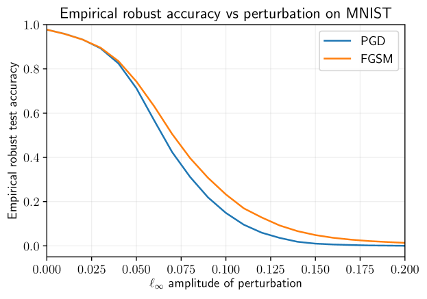
Figure 1: On the top is a plot of the certified adversarial robustness of the models trained using Lipschitz training algorithm (7) for different regularization hyperparameter $\lambda$. The top plot include the certified adversarial robustness of the MON model trained with the monotonicity parameter $m=1$. For fixed $\epsilon$, the fraction of test inputs which are certified robust are plotted. At the bottom is a plot of the empirical robustness of the implicit neural model trained with the Lipschitz training algorithm (7) with the regularization hyperparameter $\lambda=10^{-5}$ subject to the PGD and the FGSM attacks. Note the difference in scale on the horizontal axis.

In the second experiment, we train two implicit neural networks using the inclusion function training algorithm (7). For well-posedness, we impose $\mu_{\infty,[\eta]^{-1}}(W)\leq 0$ for some $\eta\in^{n}_{>0}$ and we directly parameterize $W$ as in (12). Both models are trained for $40$ epochs using the Adam optimizer and a learning rate of $5\times 10^{-4}$. At epoch $30$, the learning rate is decreased to $10^{-4}$. For the first model (shown by dashed lines in Figure 2), we set $\epsilon=\kappa=0$ during the training. This is equivalent to training a non-robust implicit neural network. For the second model (shown by solid lines in Figure 2), we pick $\epsilon_{\textup{test}}=0.1$ and $\kappa_{\textup{nom}}=0.75$. From epochs $1$ to $10$, $\kappa$ and $\epsilon$ are set to $0$ so the models undergo regular (non-robust) training. From epochs $11$ to $20$, $\epsilon$ and $\kappa$ are linearly increased such that at epoch $20$, $\epsilon=\epsilon_{\textup{test}}$ and $\kappa=\kappa_{\textup{nom}}$. Regarding the training time, using the $\alpha$-average iterations in Theorem 6.3(1), the second model takes on average 23.9 seconds to train per epoch. After training, both models are validated on test data using the sufficient conditions for certified adversarial robustness (15). For a fixed $\epsilon$ and over the 10000 test images over 10 trials, on average, it takes 11.29 seconds to compute the certified adversarial robustness using formula (15). Figure 2 provides plots for this experiment.

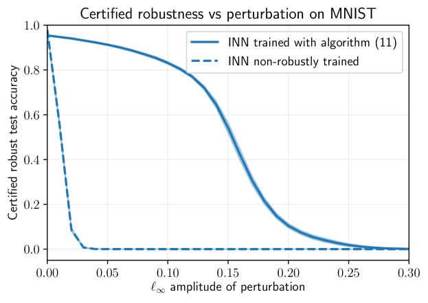
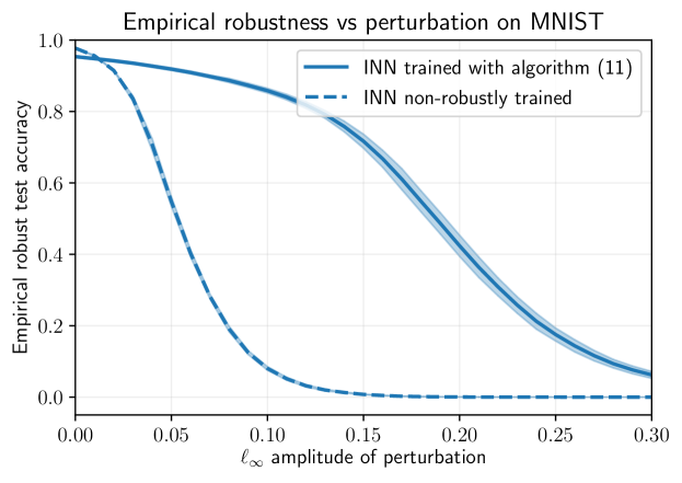
Figure 2: On the top is a plot of the certified adversarial robustness of the trained model using inclusion function training algorithm (7). At the bottom is a plot of the empirical robustness of the implicit neural model trained with inclusion function training algorithm (7) subject to the PGD attacks.

Summary evaluation.

From the first experiment, we can study the role of the regularization hyperparameter $\lambda$ in the Lipschitz training algorithm (7). From Figure 1 it is clear that increasing the value of $\lambda$ leads to increased certified robustness of the model. However, this increase is obtained at the cost of reduction in clean accuracy. Moreover, compared to the MON model (Winston & Kolter, 2020), our implicit models with regularization parameter larger than $10^{-5}$ are certifiably more robust with respect to sizable $\ell_{\infty}$-norm input perturbations. Finally, by comparing the top plot and the bottom plot in Figure 2, one can see a very large gap between the certified adversarial robustness and the empirical robustness under both PGD and FGSM attacks.

From the second experiment, we can conclude that implicit neural networks trained using the inclusion function training algorithm (7) (solid lines) vastly outperform the non-robustly trained models (the dashed line) in both certified and empirical robustness. For instance, at an $\ell_{\infty}$ perturbation radius of $0.1$, we observe that the model trained using the inclusion function training algorithm, on average, has certified robustness of $83.13\%$ and empirical robustness of $85.84\%$ with respect to PGD attack. It is worth mentioning that, at an $\ell_{\infty}$ perturbation radius of $0.1$, the non-robustly trained model has $0\%$ certified robustness and $8.04\%$ empirical robustness with respect to PGD attack.

Finally, we compare the performance of the model trained using the Lipschitz optimization algorithm (7) in Figure 1 with the model trained using the inclusion function optimization algorithm (7) in Figure 2. We can deduce that (i) the Lipschitz bound approach is significantly faster in both training the models and verification of their certified adversarial robustness and (ii) the inclusion function approach will lead to more accurate and more robust models.

9 Conclusions

Using non-Euclidean contraction theory, we develop a framework for studying robustness of implicit neural networks. For a given implicit neural network, we use estimates of (i) its $\ell_{\infty}$-norm input-output Lipschitz constant, and (ii) its tight inclusion function to obtain $\ell_{\infty}$-norm box upper bounds for input-output behavior of the network. Based on these upper bounds, we design two algorithms for training and robustness verification of implicit neural networks. Empirical evidence shows the efficiency of our algorithms.

References

- Amos & Kolter (2017) Amos, B. and Kolter, J. Z. OptNet: Differentiable optimization as a layer in neural networks. In International Conference on Machine Learning, 2017. URL https://arxiv.org/abs/1703.00443.
- Athalye et al. (2018) Athalye, A., Engstrom, L., Ilyas, A., and Kwok, K. Synthesizing robust adversarial examples. In International Conference on Machine Learning, 2018. URL https://openreview.net/forum?id=BJDH5M-AW.
- Bai et al. (2019) Bai, S., Kolter, J. Z., and Koltun, V. Deep equilibrium models. In Advances in Neural Information Processing Systems, 2019. URL https://arxiv.org/abs/1909.01377.
- Carlini & Wagner (2017) Carlini, N. and Wagner, D. Adversarial examples are not easily detected: Bypassing ten detection methods. In ACM Workshop on Artificial Intelligence and Security, pp. 3–14, 2017. doi: 10.1145/3128572.3140444.
- Chen et al. (2021) Chen, T., Lasserre, J. B., Magron, V., and Pauwels, E. Semialgebraic representation of monotone deep equilibrium models and applications to certification. In Advances in Neural Information Processing Systems, 2021. URL https://openreview.net/forum?id=m4rb1Rlfdi.
- Cohen et al. (2019) Cohen, J., Rosenfeld, E., and Kolter, J. Certified adversarial robustness via randomized smoothing. In International Conference on Machine Learning, pp. 1310–1320, 2019. URL https://arxiv.org/abs/1902.02918.
- Combettes & Pesquet (2020) Combettes, P. L. and Pesquet, J.-C. Lipschitz certificates for layered network structures driven by averaged activation operators. SIAM Journal on Mathematics of Data Science, 2(2):529–557, 2020. doi: 10.1137/19M1272780.
- Davydov et al. (2022) Davydov, A., Jafarpour, S., Abate, M., Bullo, F., and Coogan, S. Comparative analysis of interval reachability for robust implicit and feedforward neural networks. In IEEE Conf. on Decision and Control, 2022. URL https://arxiv.org/abs/2204.00187. Submitted.
- El Ghaoui et al. (2021) El Ghaoui, L., Gu, F., Travacca, B., Askari, A., and Tsai, A. Implicit deep learning. SIAM Journal on Mathematics of Data Science, 3(3):930–958, 2021. doi: 10.1137/20M1358517.
- Fazlyab et al. (2019) Fazlyab, M., Robey, A., Hassani, H., Morari, M., and Pappas, G. J. Efficient and accurate estimation of Lipschitz constants for deep neural networks. In Advances in Neural Information Processing Systems, 2019. URL https://arxiv.org/abs/1906.04893.
- Goodfellow et al. (2015) Goodfellow, I. J., Shlens, J., and Szegedy, C. Explaining and harnessing adversarial examples. In International Conference on Learning Representations, 2015. URL https://arxiv.org/abs/1412.6572.
- Gowal et al. (2018) Gowal, S., Dvijotham, K., Stanforth, R., Bunel, R., Qin, C., Uesato, J., Arandjelovic, R., Mann, T., and Kohli, P. On the effectiveness of interval bound propagation for training verifiably robust models. arXiv preprint, 2018. URL https://arxiv.org/abs/1810.12715.
- Jafarpour et al. (2021) Jafarpour, S., Davydov, A., Proskurnikov, A. V., and Bullo, F. Robust implicit networks via non-Euclidean contractions. In Advances in Neural Information Processing Systems, December 2021. URL http://arxiv.org/abs/2106.03194.
- Jafarpour et al. (2022) Jafarpour, S., Abate, M., Davydov, A., Bullo, F., and Coogan, S. Robustness certificates for implicit neural networks: A mixed monotone contractive approach. In Learning for Dynamics and Control Conference, June 2022. URL http://arxiv.org/abs/2112.05310.pdf. To appear.
- Kag et al. (2020) Kag, A., Zhang, Z., and Saligrama, V. RNNs incrementally evolving on an equilibrium manifold: A panacea for vanishing and exploding gradients? In International Conference on Learning Representations, 2020. URL https://openreview.net/forum?id=HylpqA4FwS.
- Li et al. (2019) Li, B., Chen, C., Wang, W., and Carin, L. Certified adversarial robustness with additive noise. In Advances in Neural Information Processing Systems, 2019. URL https://arxiv.org/abs/1809.03113.
- Lohmiller & Slotine (1998) Lohmiller, W. and Slotine, J.-J. E. On contraction analysis for non-linear systems. Automatica, 34(6):683–696, 1998. doi: 10.1016/S0005-1098(98)00019-3.
- Madry et al. (2018) Madry, A., Makelov, A., Schmidt, L., Tsipras, D., and Vladu, A. Towards deep learning models resistant to adversarial attacks. In International Conference on Machine Learning, 2018. URL https://arxiv.org/abs/1706.06083.
- Mirman et al. (2018) Mirman, M., Gehr, T., and Vechev, M. Differentiable abstract interpretation for provably robust neural networks. In International Conference on Machine Learning, 2018. URL https://proceedings.mlr.press/v80/mirman18b.html.
- Pabbaraju et al. (2021) Pabbaraju, C., Winston, E., and Kolter, J. Z. Estimating Lipschitz constants of monotone deep equilibrium models. In International Conference on Learning Representations, 2021. URL https://openreview.net/forum?id=VcB4QkSfyO.
- Papernot et al. (2016) Papernot, N., McDaniel, P., Wu, X., Jha, S., and Swami, A. Distillation as a defense to adversarial perturbations against deep neural networks. In IEEE Symposium on Security and Privacy, pp. 582–597, 2016. doi: 10.1109/SP.2016.41.
- Revay et al. (2020) Revay, M., Wang, R., and Manchester, I. R. Lipschitz bounded equilibrium networks. arXiv preprint arXiv:2010.01732, 2020. URL https://arxiv.org/abs/2010.01732.
- Scaman & Virmaux (2018) Scaman, K. and Virmaux, A. Lipschitz regularity of deep neural networks: Analysis and efficient estimation. In International Conference on Neural Information Processing Systems, 2018. URL https://dl.acm.org/doi/10.5555/3327144.3327299.
- Szegedy et al. (2014) Szegedy, C., Zaremba, W., Sutskever, I., Bruna, J., Erhan, D., Goodfellow, I., and Fergus, R. Intriguing properties of neural networks. In International Conference on Learning Representations, 2014. URL https://arxiv.org/abs/1312.6199.
- Wei & Kolter (2022) Wei, C. and Kolter, J. Z. Certified robustness for deep equilibrium models via interval bound propagation. In International Conference on Learning Representations, 2022. URL https://openreview.net/forum?id=y1PXylgrXZ.
- Winston & Kolter (2020) Winston, E. and Kolter, J. Z. Monotone operator equilibrium networks. In Advances in Neural Information Processing Systems, 2020. URL https://arxiv.org/abs/2006.08591.
- Wong & Kolter (2018) Wong, E. and Kolter, J. Z. Provable defenses against adversarial examples via the convex outer adversarial polytope. In International Conference on Machine Learning, pp. 5286–5295, 2018. URL http://proceedings.mlr.press/v80/wong18a.html.
- Zhang et al. (2018) Zhang, H., Weng, T.-W., Chen, P.-Y., Hsieh, C.-J., and Daniel, L. Efficient neural network robustness certification with general activation functions. In Advances in Neural Information Processing Systems, 2018. URL https://arxiv.org/abs/1811.00866.
- Zhang et al. (2020) Zhang, H., Chen, H., Xiao, C., Gowal, S., Stanforth, R., Li, B., Boning, D., and Hsieh, C.-J. Towards stable and efficient training of verifiably robust neural networks. In International Conference on Learning Representations, 2020. URL https://openreview.net/forum?id=Skxuk1rFwB.