Statistical Properties of the Probabilistic Numeric
Linear Solver BayesCG

Abstract

We analyse the calibration of BayesCG under the Krylov prior, a probabilistic numeric extension of the Conjugate Gradient (CG) method for solving systems of linear equations with symmetric positive definite coefficient matrix. Calibration refers to the statistical quality of the posterior covariances produced by a solver. Since BayesCG is not calibrated in the strict existing notion, we propose instead two test statistics that are necessary but not sufficient for calibration: the $Z$-statistic and the new $S$-statistic. We show analytically and experimentally that under low-rank approximate Krylov posteriors, BayesCG exhibits desirable properties of a calibrated solver, is only slightly optimistic, and is computationally competitive with CG.

1 Introduction

We present a rigorous analysis of the probabilistic numeric solver BayesCG under the Krylov prior [8, 32] for solving systems of linear equations

$$\mathbf{A}\mathbf{x}_{*}=\mathbf{b},$$ (1)

with symmetric positive definite coefficient matrix $\mathbf{A}\in\mathbb{R}^{n\times n}$.

Probabilistic numerics.

This area [10, 18, 29] seeks to quantify the uncertainty due to limited computational resources, and to propagate these uncertainties through computational pipelines—sequences of computations where the output of one computation is the input for the next. At the core of many computational pipelines are iterative linear solvers [7, 16, 28, 31, 35], whose computational resources are limited by the impracticality of running the solver to completion. The premature termination generates uncertainty in the computed solution.

Probabilistic numeric linear solvers.

Probabilistic numeric extensions of Kry-lov space and stationary iterative methods [2, 7, 8, 11, 17, 32, 39] model the ‘epistemic uncertainty’ in a quantity of interest, which can be the matrix inverse $\mathbf{A}^{-1}$ [17, 2, 39] or the solution $\mathbf{x}_{*}$ [8, 2, 7, 11]. Our quantity of interest is the solution $\mathbf{x}_{*}$, and the ‘epistemic uncertainty’ is the uncertainty in the user’s knowledge of the true value of $\mathbf{x}_{*}$.

The probabilistic solver takes as input a prior distribution which models the initial uncertainty in $\mathbf{x}_{*}$ and then computes posterior distributions which model the uncertainty remaining after each iteration. Figure 1 depicts a prior and posterior distribution for the solution $\mathbf{x}_{*}$ of 2-dimensional linear system.

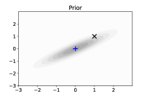
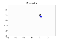
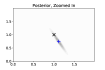
Figure 1: Prior and posterior distributions for a linear system (1) with $n=2$. Top plot: prior distribution. Bottom plots: posterior distributions, where the bottom right is a zoomed in version of the bottom left. The gray shaded contours represent the areas in which the distributions are concentrated, the symbol ‘$\times$’ represents the solution, and the symbol ‘+’ the mean of the prior or posterior.

Calibration.

An important criterion of probabilistic solvers is the statistical quality of their posterior distributions. A solver is ‘calibrated’ if its posterior distributions accurately model the uncertainty in $\mathbf{x}_{*}$ [8, Section 6.1]. Probabilistic Krylov solvers are not always calibrated because their posterior distributions tend to be pessimistic. This means, the posteriors imply that the error is larger than it actually is [2, Section 6.4], [8, Section 6.1]. Previous efforts for improving calibration have focused on scaling the posterior covariances [8, Section 4.2], [11, Section 7], [39, Section 3].

BayesCG.

We analyze the calibration of BayesCG under the Krylov prior [8, 32]. BayesCG was introduced in [8] as a probabilistic numeric extension of the Conjugate Gradient (CG) method [19] for solving (1). The Krylov prior proposed in [32] makes BayesCG competitive with CG. The numerical properties of BayesCG under the Krylov prior are analysed in [32], while here we analyse its statistical properties.

1.1 Contributions and Overview

Overall Conclusion.

BayesCG under the Krylov prior is not calibrated in the strict sense, but has the desirable properties of a calibrated solver. Under the efficient approximate Krylov posteriors, BayesCG is only slightly optimistic and competitive with CG.

Background (Section 2).

We present a short review of BayesCG, and the Krylov prior and posteriors.

Approximate Krylov posteriors (Section 3).

We define the $\mathbf{A}$-Wasserstein distance (Definition 5, Theorem 3.1); determine the error between Krylov posteriors and their low-rank approximations in the $\mathbf{A}$-Wasserstein distance (Theorem 3.2); and present a statistical interpretation of a Krylov prior as an empirical Bayesian procedure (Theorem 3.3, Remark 4).

Calibration (Section 4).

We review the strict notion of calibration for probabilistic solvers (Definition 6, Lemma 3), and show that it does not apply to BayesCG under the Krylov prior (Remark 6).

We relax the strict notion above and propose as an alternative form of assessment two test statistics that are necessary but not sufficient for calibration: the $Z$-statistic (Theorem 4.1) and the new $S$-statistic (Theorem 4.3, Definition 10). We present implementations for both (Algorithms 3 and 4); and apply a Kolmogorov-Smirnov statistic (Definition 9) for evaluating the quality of samples from the $Z$-statistic.

The $Z$-statistic is inconclusive about the calibration of BayesCG under the Krylov prior (Theorem 4.2), while the $S$-statistic indicates that it is not calibrated (Section 4.3.4).

Numerical Experiments (Section 5).

We create a calibrated but slowly converging version of BayesCG which has random search directions, and use it as a baseline for comparison with two BayesCG versions that both replicate CG: BayesCG under the inverse and the Krylov priors.

We assess calibration with the $Z$- and $S$-statistics for BayesCG with random search directions (Algorithms 5 and 6); BayesCG under the inverse prior (Algorithms 1 and 7); and BayesCG under the Krylov prior with full posteriors (Algorithm 8) and approximate posteriors (Algorithm 9).

Both, $Z$- and $S$ statistics indicate that BayesCG with random search directions is indeed a calibrated solver, while BayesCG under the inverse prior is pessimistic.

The $S$-statistic indicates that BayesCG under full Krylov posteriors mimics a calibrated solver, and that BayesCG under rank-50 approximate posteriors does as well, although not as much, since it is slightly optimistic.

1.2 Notation

Matrices are represented in bold uppercase, such as $\mathbf{A}$; vectors in bold lowercase, such as $\mathbf{b}$; and scalars in lowercase, such as $m$.

The $m\times m$ identity matrix is $\mathbf{I}_{m}$, or just $\mathbf{I}$ if the dimension is clear. The Moore-Penrose inverse of a matrix $\mathbf{A}$ is $\mathbf{A}^{\dagger}$, and the matrix square root is $\mathbf{A}^{1/2}$ [20, Chapter 6].

Probability distributions are represented in lowercase Greek, such as $\mu_{m}$; and random variables in uppercase, such as $X$. The random variable $X$ having distribution $\mu$ is represented by $X\sim\mu$, and its expectation by $\operatorname{\mathbb{E}}[X]$.

The Gaussian distribution with mean $\mathbf{x}\in\mathbb{R}^{n}$ and covariance $\mathbf{\Sigma}\in\mathbb{R}^{n\times n}$ is denoted by $\operatorname{\mathcal{N}}(\mathbf{x},\mathbf{\Sigma})$, and the chi-squared distribution with $f$ degrees of freedom by $\chi_{f}^{2}$.

2 Review of Existing Work

We review BayesCG (Section 2.1), the ideal Krylov prior (Section 2.2), and practical approximations for Krylov posteriors (Section 2.3). All statements in this section hold in exact arithmetic.

2.1 BayesCG

We review the computation of posterior distributions for BayesCG under general priors (Theorem 2.1), and present a pseudo code for BayesCG (Algorithm 1).

Given an initial guess $\mathbf{x}_{0}$, BayesCG [8] solves symmetric positive definite linear systems (1) by computing iterates $\mathbf{x}_{m}$ that converge to the solution $\mathbf{x}_{*}$. In addition, BayesCG computes probability distributions that quantify the uncertainty about the solution at each iteration $m$. Specifically, for a user-specified Gaussian prior $\mu_{0}\equiv\operatorname{\mathcal{N}}(\mathbf{x}_{0},\mathbf{\Sigma}_{0})$, BayesCG computes posterior distributions $\mu_{m}\equiv\operatorname{\mathcal{N}}(\mathbf{x}_{m},\mathbf{\Sigma}_{m})$, by conditioning a random variable $X\sim\mu_{0}$ on information from $m$ search directions $\mathbf{S}_{m}$.

Theorem 2.1 ([8, Proposition 1], [32, Theorem 2.1])

Let $\mathbf{A}\mathbf{x}_{*}=\mathbf{b}$ be a linear system where $\mathbf{A}\in\mathbb{R}^{n\times n}$ is symmetric positive definite. Let $\mu_{0}\equiv\operatorname{\mathcal{N}}(\mathbf{x}_{0},\mathbf{\Sigma}_{0})$ be a prior with symmetric positive semi-definite covariance $\mathbf{\Sigma}_{0}\in\mathbb{R}^{n\times n}$, and initial residual $\mathbf{r}_{0}\equiv\mathbf{b}_{0}-\mathbf{A}\mathbf{x}_{0}$.

Pick $m\leq n$ so that $\mathbf{S}_{m}\equiv\begin{bmatrix}\mathbf{s}_{1}&\mathbf{s}_{2}&\cdots&\mathbf{s}_{m}\end{bmatrix}\in\mathbb{R}^{n\times m}$ has $\operatorname{rank}(\mathbf{S}_{m})=m$ and $\mathbf{\Lambda}_{m}\equiv\mathbf{S}_{m}^{T}\mathbf{A}\mathbf{\Sigma}_{0}\mathbf{A}\mathbf{S}$ is non-singular. Then, the BayesCG posterior $\mu_{m}\equiv\operatorname{\mathcal{N}}(\mathbf{x}_{m},\mathbf{\Sigma}_{m})$ has mean and covariance

$$\mathbf{x}_{m} =\mathbf{x}_{0}+\mathbf{\Sigma}_{0}\mathbf{A}\mathbf{S}_{m}\mathbf{\Lambda}_{m}^{-1}\mathbf{S}_{m}^{T}\mathbf{r}_{0}$$ (2)

$$\mathbf{\Sigma}_{m} =\mathbf{\Sigma}_{0}-\mathbf{\Sigma}_{0}\mathbf{A}\mathbf{S}_{m}\mathbf{\Lambda}_{m}^{-1}\mathbf{S}_{m}^{T}\mathbf{A}\mathbf{\Sigma}_{0}.$$ (3)

Algorithm 1 represents the iterative computation of the posteriors from [8, Propositions 6 and 7], [32, Theorem 2.7]. To illustrate the resemblance of BayesCG and the Conjugate Gradient method, we present the most common implementation of CG in Algorithm 2.

BayesCG (Algorithm 1) computes specific search directions $\mathbf{S}_{m}$ with two additional properties:

1. They are $\mathbf{A}\mathbf{\Sigma}_{0}\mathbf{A}$-orthogonal, which means that $\mathbf{\Lambda}_{m}=\mathbf{S}_{m}^{T}\mathbf{A}\mathbf{\Sigma}_{0}\mathbf{A}\mathbf{S}_{m}$ is diagonal [8, Section 2.3], thus easy to invert.

2. They form a basis for the Krylov space [9, Proposition S4]

   $$\operatorname{range}(\mathbf{S}_{m})=\mathcal{K}_{m}(\mathbf{A}\mathbf{\Sigma}_{0}\mathbf{A},\mathbf{r}_{0})\equiv\operatorname{span}\{\mathbf{r}_{0},\mathbf{A}\mathbf{\Sigma}_{0}\mathbf{A}\mathbf{r}_{0},\ldots,(\mathbf{A}\mathbf{\Sigma}_{0}\mathbf{A})^{m-1}\mathbf{r}_{0}\}.$$

Remark 1

The additional requirement $\mathbf{x}_{*}-\mathbf{x}_{0}\in\operatorname{range}(\mathbf{\Sigma}_{0})$ in Algorithm 1 ensures the nonsingularity of $\mathbf{\Lambda}_{m}$ as required by Theorem 2.1, even for singular prior covariance matrices $\mathbf{\Sigma}_{0}$ [32, Theorem 2.7].

Algorithm 1 BayesCG [32, Algorithm 2.1]

1:Input: spd $\mathbf{A}\in\mathbb{R}^{n\times n}$, $\mathbf{b}\in\mathbb{R}^{n}$, prior $\mu_{0}=\operatorname{\mathcal{N}}(\mathbf{x}_{0},\mathbf{\Sigma}_{0})$ $\triangleright$ with $\mathbf{x}_{*}-\mathbf{x}_{0}\in\operatorname{range}(\mathbf{\Sigma}_{0})$

2:$\mathbf{r}_{0}=\mathbf{b}-\mathbf{A}\mathbf{x}_{0}$ $\triangleright$ Initial residual

3:$\mathbf{s}_{1}=\mathbf{r}_{0}$ $\triangleright$ Initial search direction

4:$m=0$ $\triangleright$ Initial iteration count

5:while not converged do

6:     $m=m+1$$\triangleright$ Increment iteration count

7:     $\alpha_{m}=\left(\mathbf{r}_{m-1}^{T}\mathbf{r}_{m-1}\right)\big{/}\left(\mathbf{s}_{m}^{T}\mathbf{A}\mathbf{\Sigma}_{0}\mathbf{A}\mathbf{s}_{m}\right)$

8:     $\mathbf{x}_{m}=\mathbf{x}_{m-1}+\alpha_{m}\mathbf{\Sigma}_{0}\mathbf{A}\mathbf{s}_{m}$ $\triangleright$ Next posterior mean

9:     $\mathbf{\Sigma}_{m}=\mathbf{\Sigma}_{m-1}-\mathbf{\Sigma}_{0}\mathbf{A}\mathbf{s}_{m}\left(\mathbf{\Sigma}_{0}\mathbf{A}\mathbf{s}_{m}\right)^{T}\big{/}(\mathbf{s}_{m}^{T}\mathbf{A}\mathbf{\Sigma}_{0}\mathbf{A}\mathbf{s}_{m})$ $\triangleright$ Next posterior covariance

10:     $\mathbf{r}_{m}=\mathbf{r}_{m-1}-\alpha_{m}\mathbf{A}\mathbf{\Sigma}_{0}\mathbf{A}\mathbf{s}_{m}$ $\triangleright$ Next residual

11:     $\beta_{m}=\left(\mathbf{r}_{m}^{T}\mathbf{r}_{m}\right)\big{/}\left(\mathbf{r}_{m-1}^{T}\mathbf{r}_{m-1}\right)$

12:     $\mathbf{s}_{m+1}=\mathbf{r}_{m}+\beta_{m}\mathbf{s}_{m}$ $\triangleright$ Next $\mathbf{A}\mathbf{\Sigma}_{0}\mathbf{A}$-orthogonal search direction

13:end while

14:Output: $\mu_{m}=\operatorname{\mathcal{N}}(\mathbf{x}_{m},\mathbf{\Sigma}_{m})$$\triangleright$ Final posterior

Algorithm 2 Conjugate Gradient Method (CG) [19, Section 3]

1:Input: spd $\mathbf{A}\in\mathbb{R}^{n\times n}$, $\mathbf{b}\in\mathbb{R}^{n}$, $\mathbf{x}_{0}\in\mathbb{R}^{n}$

2:$\mathbf{r}_{0}=\mathbf{b}-\mathbf{A}\mathbf{x}_{0}$ $\triangleright$ Initial residual

3:$\mathbf{w}_{1}=\mathbf{r}_{0}$ $\triangleright$ Initial search direction

4:$m=0$ $\triangleright$ Initial iteration count

5:while Not converged do

6:     $m=m+1$ $\triangleright$ Increment iteration count

7:     $\gamma_{m}=(\mathbf{r}_{m-1}^{T}\mathbf{r}_{m-1})\big{/}(\mathbf{w}_{m}^{T}\mathbf{A}\mathbf{w}_{m})$ $\triangleright$ Next step size

8:     $\mathbf{x}_{m}=\mathbf{x}_{m-1}+\gamma_{m}\mathbf{w}_{m}$$\triangleright$ Next iterate

9:     $\mathbf{r}_{m}=\mathbf{r}_{m-1}-\gamma_{m}\mathbf{A}\mathbf{w}_{m}$$\triangleright$ Next residual

10:     $\delta_{m}=(\mathbf{r}_{m}^{T}\mathbf{r}_{m})\big{/}(\mathbf{r}_{m-1}^{T}\mathbf{r}_{m-1})$

11:     $\mathbf{w}_{m+1}=\mathbf{r}_{m}+\delta_{m}\mathbf{w}_{m}$ $\triangleright$ Next search direction

12:end while

13:Output: $\mathbf{x}_{m}$ $\triangleright$ Final approximation for $\mathbf{x}_{*}$

2.2 The ideal Krylov Prior

After defining the Krylov space of maximal dimension (Definition 1), we review the ideal but impractical Krylov prior (Definition 2), and discuss its construction (Lemma 1) and properties (Theorem 2.2).

Definition 1

The Krylov space of maximal dimension for Algorithm 2 is

$$\mathcal{K}_{g}(\mathbf{A},\mathbf{r}_{0})\equiv\operatorname{span}\{\mathbf{r}_{0},\mathbf{A}\mathbf{r}_{0},\ldots,\mathbf{A}^{g-1}\mathbf{r}_{0}\}.$$

Here $g\leq n$ represents the grade of $\mathbf{r}_{0}$ with respect to $\mathbf{A}\in\mathbb{R}^{n\times n}$ [25, Definition 4.2.1], or the invariance index for $(\mathbf{A},\mathbf{r}_{0})$ [4, Section 2], which is the minimum value where

$$\mathcal{K}_{g}(\mathbf{A},\mathbf{r}_{0})=\mathcal{K}_{g+i}(\mathbf{A},\mathbf{r}_{0}),\qquad i\geq 1.$$

The Krylov prior is a Gaussian distribution whose covariance is constructed from a basis for the maximal dimensional CG Krylov space.

Definition 2 ([32, Definition 3.1])

The ideal Krylov prior for $\mathbf{A}\mathbf{x}_{*}=\mathbf{b}$ is $\eta_{0}\equiv\operatorname{\mathcal{N}}(\mathbf{x}_{0},\mathbf{\Gamma}_{0})$ with symmetric positive semi-definite covariance

$$\mathbf{\Gamma}_{0}\equiv\mathbf{V}\mathbf{\Phi}\mathbf{V}^{T}\in\mathbb{R}^{n\times n}.$$ (4)

The columns of $\mathbf{V}\equiv\begin{bmatrix}\mathbf{v}_{1}&\mathbf{v}_{2}&\cdots&\mathbf{v}_{g}\end{bmatrix}\in\mathbb{R}^{n\times g}$ are an $\mathbf{A}$-orthonormal basis for $\mathcal{K}_{g}(\mathbf{A},\mathbf{r}_{0})$, which means that

$$\mathbf{V}^{T}\mathbf{A}\mathbf{V}=\mathbf{I}_{g}\quad\text{and}\quad\operatorname{span}\{\mathbf{v}_{1},\ldots,\mathbf{v}_{i}\}=\mathcal{K}_{i}(\mathbf{A},\mathbf{r}_{0}),\quad 1\leq i\leq g.$$

The diagonal matrix $\mathbf{\Phi}\equiv\operatorname{diag}\begin{pmatrix}\phi_{1}&\cdots&\phi_{g}\end{pmatrix}\in\mathbb{R}^{g\times g}$ has diagonal elements

$$\phi_{i}=(\mathbf{v}_{i}^{T}\mathbf{r}_{0})^{2},\qquad 1\leq i\leq g.$$ (5)

Remark 2

The Krylov prior covariance satisfies the requirement of Algorithm 1 that $\mathbf{x}_{*}-\mathbf{x}_{0}\in\operatorname{range}(\mathbf{\Gamma}_{0})$. This follows from [25, Section 5.6],

$$\mathbf{x}_{*}\in\mathbf{x}_{0}+\mathcal{K}_{g}(\mathbf{A},\mathbf{r}_{0})=\operatorname{range}(\mathbf{\Gamma}_{0}).$$

If the maximal Krylov space $\mathcal{K}_{g}(\mathbf{A},\mathbf{r}_{0})$ has dimension $g<n$, then $\mathbf{\Gamma}_{0}$ is singular.

Lemma 1 ([32, Remark SM2.1])

The Krylov prior $\mathbf{\Gamma}_{0}$ can be constructed from quantities computed by CG (Algorithm 2),

$$\mathbf{v}_{i}\equiv\mathbf{w}_{i}/(\mathbf{w}_{i}^{T}\mathbf{A}\mathbf{w}_{i}),\quad\text{and}\quad\phi_{i}\equiv\gamma_{i}\|\mathbf{r}_{i-1}\|_{2}^{2},\qquad 1\leq i\leq g.$$

The posterior distributions from BayesCG under the Krylov prior depend on submatrices of $\mathbf{V}$ and $\mathbf{\Phi}$,

$$\begin{split}\mathbf{V}_{i:j}&\equiv\begin{bmatrix}\mathbf{v}_{i}&\cdots&\mathbf{v}_{j}\end{bmatrix}\\ \mathbf{\Phi}_{i:j}&\equiv\operatorname{diag}\begin{pmatrix}\phi_{i}&\cdots&\phi_{j}\end{pmatrix},\qquad 1\leq i\leq j\leq g,\end{split}$$ (6)

where $\mathbf{V}_{1:g}=\mathbf{V}$, $\mathbf{\Phi}_{1:g}=\mathbf{\Phi}$, and $\mathbf{V}_{j+1:j}=\mathbf{\Phi}_{j+1:j}=\mathbf{0}$, $1\leq j\leq n$.

Under suitable assumptions, BayesCG (Algorithm 1) produces the same iterates as CG (Algorithm 2).

Theorem 2.2 ([32, Theorem 3.3])

Let $\mathbf{x}_{0}$ be the starting vector for CG (Algorithm 2). Then BayesCG (Algorithm 1) under the Krylov prior $\eta_{0}\equiv\operatorname{\mathcal{N}}(\mathbf{x}_{0},\mathbf{\Gamma}_{0})$ produces Krylov posteriors $\eta_{m}\equiv\mathcal{N}(\mathbf{x}_{m},\mathbf{\Gamma}_{m})$ whose mean vectors

$$\mathbf{x}_{m}=\mathbf{x}_{0}+\mathbf{V}_{1:m}\mathbf{V}_{1:m}^{T}\mathbf{r}_{0},\qquad 1\leq m\leq g,$$

are identical to the iterates in CG (Algorithm 2), and whose covariance matrices

$$\mathbf{\Gamma}_{m}=\mathbf{V}_{m+1:g}\mathbf{\Phi}_{m+1:g}\mathbf{V}_{m+1:g}^{T},\qquad 1\leq m<g,$$ (7)

satisfy

$$\operatorname{trace}(\mathbf{A}\mathbf{\Gamma}_{m})=\operatorname{trace}(\mathbf{\Phi}_{m+1:g})=\|\mathbf{x}_{*}-\mathbf{x}_{m}\|_{\mathbf{A}}^{2}.$$ (8)

Explicit construction of the ideal Krylov prior, followed by explicit computation of the Krylov posteriors in Algorithm 1 is impractical, because it is more expensive than solving the linear system (1) in the first place. That is the reason for introducing practical, approximate Krylov posteriors.

2.3 Practical Krylov posteriors

We dispense with the explicit computation of the Krylov prior, and instead compute a low-rank approximation of the final posterior (Definition 3) by running $d$ additional iterations. The corresponding CG-based implementation of BayesCG under approximate Krylov posteriors is relegated to Algorithm 9 in Appendix B.

Definition 3 ([32, Definition 3.4])

Given the Krylov prior $\eta_{0}\equiv\mathcal{N}(\mathbf{x}_{0},\mathbf{\Gamma}_{0})$ with posteriors $\eta_{m}\equiv\mathcal{N}(\mathbf{x}_{m},\mathbf{\Gamma}_{m})$, pick some $d\geq 1$. The rank-$d$ approximation of $\eta_{m}$ is a Gaussian distribution $\widehat{\eta}_{m}\equiv\operatorname{\mathcal{N}}(\mathbf{x}_{m},\widehat{\mathbf{\Gamma}}_{m})$ with the same mean $\mathbf{x}_{m}$ as $\eta_{m}$, and a rank-$d$ covariance

$$\widehat{\mathbf{\Gamma}}_{m}\equiv\mathbf{V}_{m+1:m+d}\mathbf{\Phi}_{m+1:m+d}\,\mathbf{V}_{m+1:m+d}^{T},\qquad 1\leq m<g-d,$$

that consists of the leading $d$ columns of $\mathbf{V}_{m+1:g}$.

In contrast to the full Krylov posteriors, which reproduce the error as in (8), approximate Krylov posteriors underestimate the error [32, Section 3.4],

$$\operatorname{trace}(\mathbf{A}\widehat{\mathbf{\Gamma}}_{m})=\operatorname{trace}(\mathbf{\Phi}_{m+1:m+d})=\|\mathbf{x}_{*}-\mathbf{x}_{m}\|_{\mathbf{A}}^{2}-\|\mathbf{x}_{*}-\mathbf{x}_{m+d}\|_{\mathbf{A}}^{2},$$ (9)

where $\|\mathbf{x}_{*}-\mathbf{x}_{m+d}\|_{\mathbf{A}}^{2}$ is the error after $m+d$ iterations of CG. The error underestimate $\operatorname{trace}(\mathbf{A}\widehat{\mathbf{\Gamma}}_{m})$ is equal to [36, Equation(4.9)], and it is more accurate when convergence is fast. Fast convergence makes $\operatorname{trace}(\mathbf{A}\widehat{\mathbf{\Gamma}}_{m})$ a more accurate estimate because fast convergence implies that $\|\mathbf{x}_{*}-\mathbf{x}_{m+d}\|_{\mathbf{A}}^{2}\ll\|\mathbf{x}_{*}-\mathbf{x}_{m}\|_{\mathbf{A}}^{2}$, and this, along with (9), implies that $\operatorname{trace}(\mathbf{A}\widehat{\mathbf{\Gamma}}_{m})\approx\|\mathbf{x}_{*}-\mathbf{x}_{m}\|_{\mathbf{A}}^{2}$ [36, Section 4].

3 Approximate Krylov Posteriors

We determine the error in approximate Krylov posteriors (Section 3.1), and interpret the Krylov prior as an empirical Bayesian method (Section 3.2).

3.1 Error in Approximate Krylov Posteriors

We review the $p$-Wasserstein distance (Definition 4), extend the 2-Wasserstein distance to the $\mathbf{A}$-Wasserstein distance weighted by a symmetric positive definite matrix $\mathbf{A}$ (Theorem 3.1), and derive the $\mathbf{A}$-Wasserstein distance between approximate and full Krylov posteriors (Theorem 3.2).

The $p$-Wasserstein distance is a metric on the set of probability distributions.

Definition 4 ([24, Definition 2.1], [38, Definition 6.1])

The $p$-Wasser-stein distance between probability distributions $\mu$ and $\nu$ on $\mathbb{R}^{n}$ is

$$W_{p}(\mu,\nu)\equiv\left(\inf_{\pi\in\Pi(\mu,\nu)}\int_{\mathbb{R}^{n}\times\mathbb{R}^{n}}\|M-N\|_{2}^{p}\ d\pi(M,N)\right)^{1/p},\quad p\geq 1,$$ (10)

where $\Pi(\mu,\nu)$ is the set of couplings between $\mu$ and $\nu$, that is, the set of probability distributions on $\mathbb{R}^{n}\times\mathbb{R}^{n}$ that have $\mu$ and $\nu$ as marginal distributions.

In the special case $p=2$, the $2$-Wasserstein or Fréchet distance between two Gaussian distributions admits an explicit expression.

Lemma 2 ([12, Theorem 2.1])

The 2-Wasserstein distance between Gaussian distributions $\mu\equiv\operatorname{\mathcal{N}}(\mathbf{x}_{\mu},\mathbf{\Sigma}_{\mu})$ and $\nu\equiv\operatorname{\mathcal{N}}(\mathbf{x}_{\nu},\mathbf{\Sigma}_{\nu})$ on $\mathbb{R}^{n}$ is

$$\left(W_{2}(\mu,\nu)\right)^{2}=\|\mathbf{x}_{\mu}-\mathbf{x}_{\nu}\|_{2}^{2}+\operatorname{trace}\left(\mathbf{\Sigma}_{\mu}+\mathbf{\Sigma}_{\nu}-2\left(\mathbf{\Sigma}_{\mu}^{1/2}\mathbf{\Sigma}_{\nu}\mathbf{\Sigma}_{\mu}^{1/2}\right)^{1/2}\right).$$

We generalize the 2-Wasserstein distance to the $\mathbf{A}$-Wasserstein distance weighted by a symmetric positive definite matrix $\mathbf{A}$.

Definition 5

The two-norm of $\mathbf{x}\in\mathbb{R}^{n}$ weighted by a symmetric positive definite $\mathbf{A}\in\mathbb{R}^{n\times n}$ is

$$\|\mathbf{x}\|_{\mathbf{A}}\equiv\|\mathbf{A}^{1/2}\mathbf{x}\|_{2}.$$ (11)

The $\mathbf{A}$-Wasserstein distance between Gaussian distributions $\mu\equiv\operatorname{\mathcal{N}}(\mathbf{x}_{\mu},\mathbf{\Sigma}_{\mu})$ and $\nu\equiv\operatorname{\mathcal{N}}(\mathbf{x}_{\nu},\mathbf{\Sigma}_{\nu})$ on $\mathbb{R}^{n}$ is

$$W_{\mathbf{A}}(\mu,\nu)\equiv\left(\inf_{\pi\in\Pi(\mu,\nu)}\int_{\mathbb{R}^{n}\times\mathbb{R}^{n}}\|M-N\|_{\mathbf{A}}^{2}\ d\pi(M,N)\right)^{1/2},$$ (12)

where $\Pi(\mu,\nu)$ is the set of couplings between $\mu$ and $\nu$.

We derive an explicit expression for the $\mathbf{A}$-Wasserstein distance analogous to the one for the 2-Wasserstein distance in Lemma 2.

Theorem 3.1

For symmetric positive definite $\mathbf{A}\in\mathbb{R}^{n\times n}$, the $\mathbf{A}$-Wasserstein distance between Gaussian distributions $\mu\equiv\operatorname{\mathcal{N}}(\mathbf{x}_{\mu},\mathbf{\Sigma}_{\mu})$ and $\nu\equiv\operatorname{\mathcal{N}}(\mathbf{x}_{\nu},\mathbf{\Sigma}_{\nu})$ on $\mathbb{R}^{n}$ is

$$\left(W_{\mathbf{A}}(\mu,\nu)\right)^{2} =\|\mathbf{x}_{\mu}-\mathbf{x}_{\nu}\|_{\mathbf{A}}^{2}+\operatorname{trace}(\widetilde{\mathbf{\Sigma}}_{\mu})+\operatorname{trace}(\widetilde{\mathbf{\Sigma}}_{\nu})$$

$$\qquad-2\operatorname{trace}\left((\widetilde{\mathbf{\Sigma}}_{\mu}^{1/2}\widetilde{\mathbf{\Sigma}}_{\nu}\widetilde{\mathbf{\Sigma}}_{\mu}^{1/2})^{1/2}\right),$$ (13)

where $\widetilde{\mathbf{\Sigma}}_{\mu}\equiv\mathbf{A}^{1/2}\mathbf{\Sigma}_{\mu}\mathbf{A}^{1/2}$ and $\widetilde{\mathbf{\Sigma}}_{\nu}\equiv\mathbf{A}^{1/2}\mathbf{\Sigma}_{\nu}\mathbf{A}^{1/2}$.

Proof

First express the $\mathbf{A}$-Wasserstein distance as a 2-Wasserstein distance, by substituting (11) into (12),

$$\left(W_{\mathbf{A}}(\mu,\nu)\right)^{2}=\inf_{\pi\in\Pi(\mu,\nu)}\int_{\mathbb{R}^{n}\times\mathbb{R}^{n}}\|\mathbf{A}^{1/2}M-\mathbf{A}^{1/2}N\|_{2}^{2}\ d\pi(M,N).$$ (14)

Lemma 5 in Appendix A implies that $\mathbf{A}^{1/2}M$ and $\mathbf{A}^{1/2}N$ are again Gaussian random variables with respective means and covariances

$$\tilde{\mu}\equiv\mathcal{N}(\mathbf{A}^{1/2}\mathbf{x}_{\mu},\,\underbrace{\mathbf{A}^{1/2}\mathbf{\Sigma}_{\mu}\mathbf{A}^{1/2}}_{\widetilde{\mathbf{\Sigma}}_{\mu}}),\qquad\tilde{\nu}\equiv\mathcal{N}(\mathbf{A}^{1/2}\mathbf{x}_{\nu},\,\underbrace{\mathbf{A}^{1/2}\mathbf{\Sigma}_{\nu}\mathbf{A}^{1/2}}_{\widetilde{\mathbf{\Sigma}}_{\nu}}).$$

Thus (14) is equal to the 2-Wasserstein distance

$$\left(W_{\mathbf{A}}(\mu,\nu)\right)^{2}=\inf_{\pi\in\Pi(\tilde{\mu},\tilde{\nu})}\int_{\mathbb{R}^{n}\times\mathbb{R}^{n}}\|\widetilde{M}-\widetilde{N}\|_{2}^{2}\ d\pi(\widetilde{M},\widetilde{N})=\left(W_{2}(\tilde{\mu},\tilde{\nu})\right)^{2}.$$ (15)

At last, apply Lemma 2 and the linearity of the trace.∎

We are ready to derive the $\mathbf{A}$-Wasserstein distance between approximate and full Krylov posteriors.

Theorem 3.2

Let $\eta_{m}\equiv\operatorname{\mathcal{N}}(\mathbf{x}_{m},\mathbf{\Gamma}_{m})$ be a Krylov posterior from Theorem 2.2, and for some $d\geq 1$ let $\widehat{\eta}_{m}\equiv\operatorname{\mathcal{N}}(\mathbf{x}_{m},\widehat{\mathbf{\Gamma}}_{m})$ be a rank-$d$ approximation from Definition 3. The $\mathbf{A}$-Wasserstein distance between $\eta_{m}$ and $\widehat{\eta}_{m}$ is

$$W_{\mathbf{A}}(\eta_{m},\widehat{\eta}_{m})=\left(\sum_{i=m+d+1}^{g}\phi_{i}\right)^{1/2}.$$ (16)

Proof

We factor the covariances into square factors, to obtain an eigenvalue decomposition for the congruence transformations of the covariances in (3.1).

Expand the column dimension of $\mathbf{V}_{m+1:g}$ from $g-m$ to $n$ by adding an $\mathbf{A}$-orthogonal complement $\mathbf{V}_{m}^{\perp}\in\mathbb{R}^{n\times(n-g+m)}$ to create an $\mathbf{A}$-orthogonal matrix

$$\widetilde{\mathbf{V}} \equiv\begin{bmatrix}\mathbf{V}_{m+1:g}&\mathbf{V}_{m}^{\perp}\end{bmatrix}\in\mathbb{R}^{n\times n}$$

with $\widetilde{\mathbf{V}}^{T}\mathbf{A}\widetilde{\mathbf{V}}=\mathbf{I}_{n}$. Analogously expand the dimension of the diagonal matrices by padding with trailing zeros,

$$\widetilde{\mathbf{\Phi}}_{m+1:g} \equiv\operatorname{diag}\begin{pmatrix}\phi_{m+1}&\cdots&\phi_{g}&\mathbf{0}_{1\times(n-g+m)}\end{pmatrix}\in\mathbb{R}^{n\times n},$$

$$\widetilde{\mathbf{\Phi}}_{m+1:m+d} \equiv\operatorname{diag}\begin{pmatrix}\phi_{m+1}&\cdots&\phi_{m+d}&\mathbf{0}_{1\times(n-d)}\end{pmatrix}\in\mathbb{R}^{n\times n}.$$

Factor the covariances in terms of the above square matrices,

$$\mathbf{\Gamma}_{m}=\widetilde{\mathbf{V}}\widetilde{\mathbf{\Phi}}_{m+1:g}\widetilde{\mathbf{V}}^{T}\quad\text{and}\quad\widehat{\mathbf{\Gamma}}_{m}=\widetilde{\mathbf{V}}\widetilde{\mathbf{\Phi}}_{m+1:m+d}\widetilde{\mathbf{V}}^{T}.$$

Substitute the factorizations into (3.1), and compute the $\mathbf{A}$-Wasserstein distance between $\eta_{m}$ and $\widehat{\eta}_{m}$ as

$$\left(W_{\mathbf{A}}(\eta_{m},\widehat{\eta}_{m})\right)^{2}=\operatorname{trace}(\mathbf{G})+\operatorname{trace}(\mathbf{J})-2\operatorname{trace}\left((\mathbf{G}^{1/2}\,\mathbf{J}\,\mathbf{G}^{1/2})^{1/2}\right),$$ (17)

where the congruence transformations of $\mathbf{\Gamma}_{m}$ and $\widehat{\mathbf{\Gamma}}_{m}$ are again Hermitian,

$$\mathbf{G} \equiv\mathbf{A}^{1/2}\underbrace{\widetilde{\mathbf{V}}\widetilde{\mathbf{\Phi}}_{m+1:g}\widetilde{\mathbf{V}}^{T}}_{\mathbf{\Gamma}_{m}}\mathbf{A}^{1/2}=\mathbf{U}\widetilde{\mathbf{\Phi}}_{m+1:g}\mathbf{U}^{T},\qquad\mathbf{U}\equiv\mathbf{A}^{1/2}\widetilde{\mathbf{V}}$$

$$\mathbf{J} \equiv\mathbf{A}^{1/2}\underbrace{\widetilde{\mathbf{V}}\widetilde{\mathbf{\Phi}}_{m+1:m+d}\widetilde{\mathbf{V}}^{T}}_{\widehat{\mathbf{\Gamma}}_{m}}\mathbf{A}^{1/2}=\mathbf{U}\widetilde{\mathbf{\Phi}}_{m+1:d}\mathbf{U}^{T}.$$

Lemma 7 implies that $\mathbf{U}$ is an orthogonal matrix, so that the second factorizations of $\mathbf{G}$ and $\mathbf{J}$ represent eigenvalue decompositions. Commutativity of the trace implies

$$\operatorname{trace}(\mathbf{G}) =\operatorname{trace}(\widetilde{\mathbf{\Phi}}_{m+1:g})=\sum_{i=m+1}^{g}{\phi_{i}}$$

$$\operatorname{trace}(\mathbf{J}) =\operatorname{trace}(\widetilde{\mathbf{\Phi}}_{m+1:m+d})=\sum_{i=m+1}^{m+d}{\phi_{i}}.$$

Since $\mathbf{G}$ and $\mathbf{J}$ have the same eigenvector matrix, they commute, and so do diagonal matrices,

$$\mathbf{G}^{1/2}\mathbf{J}\mathbf{G}^{1/2} =\mathbf{U}\widetilde{\mathbf{\Phi}}_{m+1:g}\widetilde{\mathbf{\Phi}}_{m+1:m+d}\mathbf{U}^{T}$$

$$=\mathbf{U}\operatorname{diag}\begin{pmatrix}\phi_{m+1}^{2}&\cdots\phi_{m+d}^{2}&\mathbf{0}_{1\times(n-d)}\end{pmatrix}\mathbf{U}^{T}$$

where the last equality follows from the fact that $\widetilde{\mathbf{\Phi}}_{m+1:g}$ and $\widetilde{\mathbf{\Phi}}_{m+1:m+d}$ share the leading $d$ diagonal elements. Thus

$$\operatorname{trace}\left((\mathbf{G}^{1/2}\,\mathbf{J}\,\mathbf{G}^{1/2})^{1/2}\right)=\sum_{i=m+1}^{m+d}\phi_{i}.$$

Substituting the above expressions into (17) gives

$$\left(W_{\mathbf{A}}(\eta_{m},\widehat{\eta}_{m})\right)^{2}=\sum_{i=m+1}^{g}\phi_{i}+\sum_{i=m+1}^{m+d}\phi_{i}-2\sum_{i=m+1}^{m+d}\phi_{i}=\sum_{i=m+d+1}^{g}{\phi_{i}}.$$

∎

Theorem 3.2 implies that the $\mathbf{A}$-Wasserstein distance between approximate and full Krylov posteriors is the sum of the CG steps sizes skipped by the approximate posterior, and this, as seen in (9) and [36, Equation (4.4)], is equal to the distance between the error estimate $\operatorname{trace}(\mathbf{A}\widehat{\mathbf{\Gamma}}_{m})$ and the true error $\|\mathbf{x}_{*}-\mathbf{x}_{m}\|_{\mathbf{A}}^{2}$. As a consequence, the approximation error decreases as the convergence of the posterior mean accelerates, or the rank $d$ of the approximation increases.

Remark 3

The distance in Theorem 3.2 is a special case of the 2-Wasserstein distance between two distributions whose covariance matrices commute [24, Corollary 2.4].

To see this, consider the $\mathbf{A}$-Wasserstein distance between $\eta_{m}$ and $\widehat{\eta}_{m}$ from Theorem 3.2, and the 2-Wasserstein distance between $\nu_{m}\equiv\operatorname{\mathcal{N}}(\mathbf{x}_{m},\mathbf{A}^{1/2}\mathbf{\Gamma}\mathbf{A}^{1/2})$ and $\widehat{\nu}_{m}\equiv\operatorname{\mathcal{N}}(\mathbf{x}_{m},\mathbf{A}^{1/2}\widehat{\mathbf{\Gamma}}\mathbf{A}^{1/2})$. Then (15) implies that the $\mathbf{A}$-Wasserstein distance is equal to the 2-Wassterstein distance of a congruence transformation,

$$W_{\mathbf{A}}(\eta_{m},\widehat{\eta}_{m})=W_{2}(\nu_{m},\widehat{\nu}_{m}).$$

The covariance matrices $\mathbf{A}^{1/2}\mathbf{\Gamma}_{m}\mathbf{A}^{1/2}$ and $\mathbf{A}^{1/2}\widehat{\mathbf{\Gamma}}_{m}\mathbf{A}^{1/2}$ associated with the 2-Wasserstein distance commute because they are both diagonalized by the same orthogonal matrix $\mathbf{A}^{1/2}\widetilde{\mathbf{V}}$.

3.2 Probabilistic Interpretation of the Krylov Prior

We interpret the Krylov prior as an ‘empirical Bayesian procedure’ (Theorem 3.3), and elucidate the connection between the random variables and the deterministic solution (Remark 4).

An empirical Bayesian procedure estimates the prior from data [3, Section 4.5]. Our ‘data’ are the pairs of normalized search directions $\mathbf{v}_{i}$ and step sizes $\phi_{i}$, $1\leq i\leq m+d$, from $m+d$ iterations of CG. In contrast, the usual data for BayesCG are the inner products $\mathbf{v}_{i}^{T}\mathbf{b}$, $1\leq i\leq m$. However, if we augment the usual data with the search directions, which is natural due to their dependence on $\mathbf{x}_{*}$, then $\phi_{i}$ is just a function of the data.

From these data we construct a prior in an empirical Bayesian fashion, starting with a random variable

$$X=\mathbf{x}_{0}+\sum_{i=1}^{m+d}\sqrt{\phi_{i}}\mathbf{v}_{i}Q_{i}\in\mathbb{R}^{n},$$

where $Q_{i}\sim\operatorname{\mathcal{N}}(0,1)$ are independent and identically distributed scalar Gaussian random variables, $1\leq i\leq m+d$. Due to the independence of the $Q_{i}$, the above sum is the matrix vector product

$$X=\mathbf{x}_{0}+\mathbf{V}_{1:m+d}\,\mathbf{\Phi}_{1:m+d}^{1/2}\,Q$$ (18)

where $Q\sim\mathcal{N}(\mathbf{0},\mathbf{I}_{m+d})$ is a vector-valued Gaussian random variable.

The distribution of $X$ is the empirical prior, while the distribution of $X$ conditioned on the random variable $Y\equiv\mathbf{V}_{1:m}^{T}\mathbf{A}X$ taking the value $\mathbf{V}_{1:m}^{T}\mathbf{b}$ is the empirical posterior. We relate these distributions to the Krylov prior.

Theorem 3.3

Under the assumptions of Theorem 2.2, the random variable $X$ in (18) is distributed according to the empirical prior

$$\operatorname{\mathcal{N}}\left(\mathbf{x}_{0},\mathbf{V}_{1:m+d}\mathbf{\Phi}_{1:m+d}\mathbf{V}_{1:m+d}^{T}\right),$$

which is the rank-$(m+d)$ approximation of the Krylov prior $\mathbf{\Gamma}_{0}$. The variable $X$ conditioned on $Y\equiv\mathbf{V}_{1:m}^{T}\mathbf{A}X$ taking the value $\mathbf{V}_{1:m}^{T}\mathbf{b}$ is distributed according to the empirical posterior

$$\operatorname{\mathcal{N}}\left(\mathbf{x}_{m},\mathbf{V}_{m+1:m+d}\mathbf{\Phi}_{m+1:m+d}\mathbf{V}_{m+1:m+d}^{T}\right)=\operatorname{\mathcal{N}}\left(\mathbf{x}_{m},\widehat{\mathbf{\Gamma}}_{m}\right),$$

which, in turn, is the rank-$d$ approximation of the Krylov posterior.

Proof

As in the proof of Theorem 2.1 in [9, Proof of Proposition 1], we exploit the stability and conjugacy of Gaussian distributions in Lemmas 5 and 6 in Appendix A.

Prior.

Lemma 5 implies that $X$ in (18) is a Gaussian random variable with mean and covariance

$$X\sim\mathcal{N}\left(\mathbf{x}_{0},\mathbf{V}_{1:m+d}\mathbf{\Phi}_{1:m+d}\mathbf{V}_{1:m+d}^{T}\right).$$ (19)

Thus, the approximate Krylov prior is an empirical Bayesian prior.

Posterior.

From (19) follows that $X$ and $Y\equiv\mathbf{V}_{1:m}^{T}\mathbf{A}X$ have the joint distribution

$$\begin{bmatrix}X\\ Y\end{bmatrix}\sim\operatorname{\mathcal{N}}\left(\begin{bmatrix}\mathbf{x}_{0}\\ \operatorname{\mathbb{E}}[Y]\end{bmatrix},\begin{bmatrix}\mathbf{V}_{1:m+d}\mathbf{\Phi}_{1:m+d}\mathbf{V}_{1:m+d}^{T}&\operatorname{Cov}(X,Y)\\ \operatorname{Cov}(X,Y)^{T}&\operatorname{Cov}(Y,Y)\end{bmatrix}\right)$$ (20)

and that $\operatorname{\mathbb{E}}[Y]=\mathbf{V}_{1:m}^{T}\mathbf{A}\mathbf{x}_{0}$. This, together with the linearity of the expectation and the $\mathbf{A}$-orthonormality of $\mathbf{V}$ implies

$$\operatorname{Cov}(Y,Y) =\operatorname{\mathbb{E}}\left[(Y-\operatorname{\mathbb{E}}[Y])(Y-\operatorname{\mathbb{E}}[Y])^{T}\right]$$

$$=\mathbf{V}_{1:m}^{T}\mathbf{A}\,\operatorname{\mathbb{E}}\left[(X-\mathbf{x}_{0})(X-\mathbf{x}_{0})^{T}\right]\mathbf{A}\mathbf{V}_{1:m}$$

$$=\mathbf{V}_{1:m}^{T}\mathbf{A}\>\left(\mathbf{V}_{1:m+d}\mathbf{\Phi}_{1:m+d}\mathbf{V}_{1:m+d}^{T}\right)\>\mathbf{A}\mathbf{V}_{1:m}$$

$$=\begin{bmatrix}\mathbf{I}_{m}&\mathbf{0}\end{bmatrix}\mathbf{\Phi}_{1:m+d}\begin{bmatrix}\mathbf{I}_{m}\\ \mathbf{0}\end{bmatrix}=\mathbf{\Phi}_{1:m}.$$

Analogously,

$$\operatorname{Cov}(X,Y) =\operatorname{\mathbb{E}}[(X-\mathbf{x}_{0})(Y-\operatorname{\mathbb{E}}[Y])^{T}]=\operatorname{\mathbb{E}}[(X-\mathbf{x}_{0})(Y-\mathbf{V}_{1:m}^{T}\mathbf{A}\mathbf{x}_{0})^{T}]$$

$$=\operatorname{\mathbb{E}}[(X-\mathbf{x}_{0})(X-\mathbf{x}_{0})^{T}]\mathbf{A}\mathbf{V}_{1:m}=\mathbf{V}_{1:m+d}\mathbf{\Phi}_{1:m+d}\mathbf{V}_{1:m+d}^{T}\mathbf{A}\mathbf{V}_{1:m}$$

$$=\mathbf{V}_{1:m+d}\mathbf{\Phi}_{1:m+d}\begin{bmatrix}\mathbf{I}_{m}&\mathbf{0}\end{bmatrix}=\mathbf{V}_{1:m}\mathbf{\Phi}_{1:m}.$$

From [37, Theorem 6.20] follows the expression for the posterior mean,

$$\mathbf{x}_{m} =\mathbf{x}_{0}+\operatorname{Cov}(X,Y)\operatorname{Cov}(Y,Y)^{-1}\left(\mathbf{V}_{1:m}^{T}\mathbf{b}-\mathbf{V}_{1:m}^{T}\mathbf{A}\mathbf{x}_{0}\right)$$

$$=\mathbf{x}_{0}+\mathbf{V}_{1:m}\mathbf{\Phi}_{1:m}\mathbf{\Phi}_{1:m}^{-1}\mathbf{V}_{1:m}^{T}\mathbf{r}_{0}=\mathbf{x}_{0}+\mathbf{V}_{1:m}\mathbf{V}_{1:m}^{T}\mathbf{r}_{0},$$

and for the posterior covariance

$$\widehat{\mathbf{\Gamma}}_{m} =\mathbf{V}_{1:m+d}\mathbf{\Phi}_{1:m+d}\mathbf{V}_{1:m+d}^{T}-\operatorname{Cov}(X,Y)\operatorname{Cov}(Y,Y)^{-1}\operatorname{Cov}(X,Y)^{T},$$

where

$$\operatorname{Cov}(X,Y)\operatorname{Cov}(Y,Y)^{-1}\operatorname{Cov}(X,Y)^{T} =\mathbf{V}_{1:m}\mathbf{\Phi}_{1:m}\mathbf{\Phi}_{1:m}^{-1}\mathbf{\Phi}_{1:m}\mathbf{V}_{1:m}^{T}$$

$$=\mathbf{V}_{1:m}\mathbf{\Phi}_{1:m}\mathbf{V}_{1:m}^{T}.$$

Substituting this into $\widehat{\mathbf{\Gamma}}_{m}$ gives the expression for the posterior covariance

$$\widehat{\mathbf{\Gamma}}_{m} =\mathbf{V}_{1:m+d}\mathbf{\Phi}_{1:m+d}\mathbf{V}_{1:m+d}^{T}-\mathbf{V}_{1:m}\mathbf{\Phi}_{1:m}\mathbf{V}_{1:m}^{T}$$

$$=\mathbf{V}_{m+1:m+d}\mathbf{\Phi}_{m+1:m+d}\mathbf{V}_{m+1:m+d}^{T}.$$

Thus, the posterior mean $\mathbf{x}_{m}$ is equal to the one in Theorem 2.2, and the posterior covariance $\widehat{\mathbf{\Gamma}}_{m}$ is equal to the rank-$d$ approximate Krylov posterior in Definition 3.∎

Remark 4

The random variable $X$ in Theorem 3.3 is a surrogate for the unknown solution $\mathbf{x}_{*}$. The solution $\mathbf{x}_{*}$ is a deterministic quantity, but prior to solving the linear system (1), we are uncertain of $\mathbf{x}_{*}$, and the prior models this uncertainty.

During the course of the BayesCG iterations, we acquire information about $\mathbf{x}_{*}$, and the posterior distributions $\mu_{m}$, $1\leq m\leq n$ incorporate our increasing knowledge and, consequently, our diminishing uncertainty.

4 Calibration of BayesCG Under the Krylov Prior

We review the notion of calibration for probabilistic solvers, and show that this notion does not apply to BayesCG under the Krylov prior (Section 4.1). Then we relax this notion and analyze BayesCG with two test statistics that are necessary but not sufficient for calibration: the $Z$-statistic (Section 4.2) and the $S$-statistic (Section 4.3).

4.1 Calibration

We review the definition of calibration for probabilistic linear solvers (Definition 6, Lemma 3), discuss the difference between certain random variables (Remark 5), present two illustrations (Examples 1 and 2), and explain why this notion of calibration does not apply to BayesCG under the Krylov prior (Remark 6).

Informally, a probabilistic numerical solver is calibrated if its posterior distributions accurately model the uncertainty in the solution [6, 7].

Definition 6 ([7, Definition 6])

Let $\mathbf{A}X_{*}=B$ be a class of linear systems where $\mathbf{A}\in\mathbb{R}^{n\times n}$ is symmetric positive definite, and the random right hand sides $B\in\mathbb{R}^{n}$ are defined by random solutions $X_{*}\sim\mu_{0}\equiv\operatorname{\mathcal{N}}(\mathbf{x}_{0},\mathbf{\Sigma}_{0})$.

Assume that a probabilistic linear solver under the prior $\mu_{0}$ and applied to a system $\mathbf{A}X_{*}=B$ computes posteriors $\mu_{m}\equiv\operatorname{\mathcal{N}}(\mathbf{x}_{m},\mathbf{\Sigma}_{m})$, $1\leq m\leq n$. Let $\operatorname{rank}(\mathbf{\Sigma}_{m})=p_{m}$, and let $\mathbf{\Sigma}_{m}$ have an orthogonal eigenvector matrix $\mathbf{U}=\begin{bmatrix}\mathbf{U}_{m}&\mathbf{U}_{m}^{\perp}\end{bmatrix}\in\mathbb{R}^{n\times n}$ where $\mathbf{U}_{m}\in\mathbb{R}^{n\times p_{m}}$ and $\mathbf{U}_{m}^{\perp}\in\mathbb{R}^{n\times(n-p_{m})}$ satisfy

$$\operatorname{range}(\mathbf{U}_{m})=\operatorname{range}(\mathbf{\Sigma}_{m}),\qquad\quad\operatorname{range}(\mathbf{U}_{m}^{\perp})=\ker(\mathbf{\Sigma}_{m}).$$

The probabilistic solver is calibrated if all posterior covariances $\mathbf{\Sigma}_{m}$ are independent of $B$ and satisfy

$$\begin{split}(\mathbf{U}_{m}^{T}\mathbf{\Sigma}_{m}\mathbf{U}_{m})^{-1/2}\mathbf{U}_{m}^{T}(X_{*}-\mathbf{x}_{m})&\sim\operatorname{\mathcal{N}}(\mathbf{0},\mathbf{I}_{p_{m}}),\\ (\mathbf{U}_{m}^{\perp})^{T}(X_{*}-\mathbf{x}_{m})&=\mathbf{0},\qquad 1\leq m\leq n.\end{split}$$ (21)

Alternatively, one can think of a probabilistic linear solver as calibrated if and only if the solutions $X_{*}$ are distributed according to the posteriors.

Lemma 3

Under the conditions of Definition 6, a probabilistic linear solver is calibrated, if and only if

$$X_{*}\sim\operatorname{\mathcal{N}}(\mathbf{x}_{m},\mathbf{\Sigma}_{m}),\qquad 1\leq m\leq n.$$

Proof

Let $\mathbf{\Sigma}_{m}=\mathbf{U}\mathbf{D}\mathbf{U}^{T}$ be an eigendecomposition where the eigenvalue matrix $\mathbf{D}=\operatorname{diag}\begin{pmatrix}\mathbf{D}_{m}&\mathbf{0}\end{pmatrix}$ is commensurately partitioned with $\mathbf{U}$ in Definition 6. Multiply the first equation of (21) on the left by $\mathbf{D}_{m}=\mathbf{U}_{m}^{T}\mathbf{\Sigma}_{m}\mathbf{U}_{m}$,

$$\mathbf{U}_{m}^{T}(X_{*}-\mathbf{x}_{m})\sim\operatorname{\mathcal{N}}(\mathbf{0},\mathbf{D}_{m}),$$

combine the result with the second equation in (21),

$$\mathbf{U}^{T}(X_{*}-\mathbf{x}_{m})\sim\operatorname{\mathcal{N}}\left(\mathbf{0},\mathbf{D}\right).$$

and multiply by $\mathbf{U}$ on the left,

$$(X_{*}-\mathbf{x}_{m})\sim\operatorname{\mathcal{N}}(\mathbf{0},\mathbf{U}\mathbf{D}\mathbf{U}^{T}),\qquad 1\leq m\leq n.$$

At last, substitute $\mathbf{\Sigma}_{m}=\mathbf{U}\mathbf{D}\mathbf{U}^{T}$ and subtract $\mathbf{x}_{m}$. ∎

Since the covariance matrix $\mathbf{\Sigma}_{m}$ is singular, its probability density function is zero on the subspace of $\mathbb{R}^{n}$ where the solver has eliminated the uncertainty about $X_{*}$. From (21) follows that $X_{*}=\mathbf{x}_{m}$ in $\ker(\mathbf{\Sigma}_{m})$. Hence, this subspace must be $\ker(\mathbf{\Sigma}_{m})$, and any remaining uncertainty about $X_{*}$ lies in $\operatorname{range}(\mathbf{\Sigma}_{m})$.

Remark 5

We discuss the difference between the random variable $X_{*}$ in Definition 6 and the random variable $X$ in Theorem 3.3.

In the context of calibration, the random variable $X_{*}\sim\mu_{0}$ represents the set of all possible solutions that are accurately modeled by the prior $\mu_{0}$. If the solver is calibrated, then Lemma 3 shows that $X_{*}\sim\mu_{m}$. Thus, solutions accurately modeled by the prior $\mu_{0}$ are also accurately modeled by all posteriors $\mu_{m}$.

By contrast, in the context of a deterministic linear system $\mathbf{A}\mathbf{x}_{*}=\mathbf{b}$, the random variable $X$ represents a surrogate for the particular solution $\mathbf{x}_{*}$ and can be viewed as an abbreviation for $X\mid X_{*}=\mathbf{x}_{*}$. The prior $\mu_{0}$ models the uncertainty in the user’s initial knowledge of $\mathbf{x}_{*}$, and the posteriors $\mu_{m}$ model the uncertainty remaining after $m$ iterations of the solver.

The following two examples illustrate Definition 6.

Example 1

Suppose there are three people: Alice, Bob, and Carol.

1. Alice samples $\mathbf{x}_{*}$ from the prior $\mu_{0}$ and computes the matrix vector product $\mathbf{b}=\mathbf{A}\mathbf{x}_{*}$.

2. Bob receives $\mu_{0}$, $\mathbf{b}$, and $\mathbf{A}$ from Alice. He estimates $\mathbf{x}_{*}$ by solving the linear system with a probabilistic solver under the prior $\mu_{0}$, and then samples $\mathbf{y}$ from a posterior $\mu_{m}$.

3. Carol receives $\mu_{m}$, $\mathbf{x}_{*}$ and $\mathbf{y}$, but she is not told which vector is $\mathbf{x}_{*}$ and which is $\mathbf{y}$. Carol then attempts to determine which one of $\mathbf{x}_{*}$ or $\mathbf{y}$ is the sample from $\mu_{m}$. If Carol cannot distinguish between $\mathbf{x}_{*}$ and $\mathbf{y}$, then the solver is calibrated.

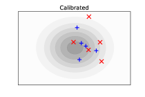
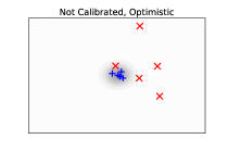
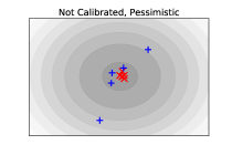
Figure 2: Posterior distributions and solutions from three different probabilistic solvers: calibrated (top), optimistic (bottom left), and pessimistic (bottom right). The gray contours represent the posterior distributions, the red symbols “$\times$” the solutions, and the blue symbols “+” samples from the posterior distributions.

Example 2

This is the visual equivalent of Example 1, where Carol receives the images in Figure 2 of three different probabilistic solvers, but without any identification of the solutions and posterior samples.

• Top plot. This solver is calibrated because the solutions look indistinguishable from the samples of the posterior distribution.

• Bottom left plot. This solver is not calibrated because the solutions are unlikely to be samples from the posterior distribution.
  The solver is optimistic because the posterior distribution is concentrated in an area of $\mathbb{R}^{n}$ that is too small to cover the solutions.

• Bottom right plot. The solver is not calibrated. Although the solutions could plausibly be sampled from the posterior, they are concentrated too close to the center of the distribution.
  The solver is pessimistic because the area covered by the posterior distribution is much larger than the area containing the solutions.

Remark 6

The posterior means and covariances from a probabilistic solver can depend on the solution $\mathbf{x}_{*}$, as is the case for BayesCG. If a solver is applied to a random linear system in Definition 6 and if the posterior means and covariances depend on the solution $X_{*}$, then the posterior means and covariances are also random variables.

Definition 6 prevents the posterior covariances from being random variables by forcing them to be independent of the random right hand side $B$. Although this is a realistic constraint for the stationary iterative solvers in [32], it does not apply to BayesCG under the Krylov prior, because Krylov posterior covariances depend non-linearly on the right-hand side. In Sections 4.2 and 4.3, we present a remedy for BayesCG in the form of test statistics that are motivated by Definition 6 and Lemma 3.

4.2 The $Z$-statistic

We assess BayesCG under the Krylov prior with an existing test statistic, the $Z$-statistic, which is a necessary condition for calibration and can be viewed as a weaker normwise version of criterion (21). We review the $Z$-statistic (Section 4.2.1), and apply it to BayesCG under the Krylov prior (Section 4.2.2).

4.2.1 Review of the $Z$-statistic

We review the $Z$-statistic (Definition 7), and the chi-square distribution (Definition 8), which links the $Z$-statistic to calibration (Theorem 4.1). Then we discuss how to generate samples of the $Z$-statistic (Algorithm 3), how to use them for the assessment of calibration (Remark 7), and then present the Kolmogorov-Smirnov statistic as a computationally inexpensive estimate for the difference between two general distributions (Definition 9).

The $Z$-statistic was introduced in [8, Section 6.1] as a means to assess the calibration of BayesCG, and has subsequently been applied to other probabilistic linear solvers [2, Section 6.4], [11, Section 9].

Definition 7 ([8, Section 6.1])

Let $\mathbf{A}X_{*}=B$ be a class of linear systems where $\mathbf{A}\in\mathbb{R}^{n\times n}$ is symmetric positive definite, and $X_{*}\sim\mu_{0}\equiv\operatorname{\mathcal{N}}(\mathbf{x}_{0},\mathbf{\Sigma}_{0})$. Let $\mu_{m}\equiv\operatorname{\mathcal{N}}(\mathbf{x}_{m},\mathbf{\Sigma}_{m})$, $1\leq m\leq n$, be the posterior distributions from a probabilistic solver under the prior $\mu_{0}$ applied to $\mathbf{A}X_{*}=B$. The $Z$-statistic is

$$\mathrm{Z}_{m}(X_{*})\equiv(X_{*}-\mathbf{x}_{m})^{T}\mathbf{\Sigma}_{m}^{\dagger}(X_{*}-\mathbf{x}_{m}),\qquad 1\leq m\leq n.$$ (22)

The chi-squared distribution below furnishes the link from $Z$-statistic to calibration.

Definition 8 ([33, Definition 2.2])

If $X_{1},\ldots,X_{f}\in\mathcal{N}(0,1)$ are independent random normal variables, then $\sum_{j=1}^{f}{X_{j}^{2}}$ is distributed according to the chi-squared distribution $\chi_{f}^{2}$ with $f$ degrees of freedom and mean $f$.
In other words, if $X\sim\operatorname{\mathcal{N}}(\mathbf{0},\mathbf{I}_{f})$, then $X^{T}X\sim\chi_{f}^{2}$ and $\operatorname{\mathbb{E}}[X^{T}X]=f$.

We show that the $Z$-statistic is a necessary condition for calibration. That is: If a probabilistic solver is calibrated, then the $Z$-statistic is distributed according to a chi-squared distribution.

Theorem 4.1 ([9, Proposition 1])

Let $\mathbf{A}X_{*}=B$ be a class of linear systems where $\mathbf{A}\in\mathbb{R}^{n\times n}$ is symmetric positive definite, and $X_{*}\sim\mu_{0}\equiv\operatorname{\mathcal{N}}(\mathbf{x}_{0},\mathbf{\Sigma}_{0})$. Assume that a probabilistic solver under the prior $\mu_{0}$ applied to $\mathbf{A}X_{*}=B$ computes the posteriors $\mu_{m}\equiv\operatorname{\mathcal{N}}(\mathbf{x}_{m},\mathbf{\Sigma}_{m})$ with $\operatorname{rank}(\mathbf{\Sigma}_{m})=p_{m}$, $1\leq m\leq n$.

If the solver is calibrated, then

$$\mathrm{Z}_{m}(X_{*})\sim\chi_{p_{m}}^{2},\qquad 1\leq m\leq n.$$

Proof

Write $\mathrm{Z}_{m}(X_{*})=M_{m}^{T}M_{m}$, where $M_{m}\equiv(\mathbf{\Sigma}_{m}^{\dagger})^{1/2}(X_{*}-\mathbf{x}_{m})$. Lemma 3 implies that a calibrated solver produces posteriors with

$$(X_{*}-\mathbf{x}_{m})\sim\operatorname{\mathcal{N}}(\mathbf{0},\mathbf{\Sigma}_{m}),\qquad 1\leq m\leq n.$$

With the eigenvector matrix $\mathbf{U}_{m}\in\mathbb{R}^{n\times p_{m}}$ as in Definition 6, Lemma 5 in Appendix A implies

$$M_{m}\sim\operatorname{\mathcal{N}}(\mathbf{0},\mathbf{U}_{m}\mathbf{U}_{m}^{T}),\qquad 1\leq m\leq n.$$

Since the covariance of $M_{m}$ is an orthogonal projector, Lemma 10 implies $\mathrm{Z}_{m}(X_{*})=(M_{m}^{T}M_{m})\sim\chi_{p_{m}}^{2}$. ∎

Theorem 4.1 implies that BayesCG is calibrated if the $Z$-statistic is distributed according to a chi-squared distribution with $p_{m}=\operatorname{rank}(\mathbf{\Sigma}_{0})-m$ degrees of freedom. For the Krylov prior specifically, $p_{m}=g-m$.

Generating samples from the $Z$-statistic and assessing calibration.

For a user-specified probabilistic linear solver and a symmetric positive definite matrix $\mathbf{A}$, Algorithm 3 samples $N_{\text{test}}$ solutions $\mathbf{x}_{*}$ from the prior distribution $\mu_{0}$, defines the systems $\mathbf{b}\equiv\mathbf{A}\mathbf{x}_{*}$, runs $m$ iterations of the solver on $\mathbf{b}\equiv\mathbf{A}\mathbf{x}_{*}$, and computes $\mathrm{Z}_{m}(\mathbf{x}_{*})$ in (22).

The application of the Moore-Penrose inverse in Line 6 can be implemented by computing the minimal norm solution $\mathbf{q}=\mathbf{\Sigma}_{m}^{\dagger}(\mathbf{x}_{*}-\mathbf{x}_{m})$ of the least squares problem

$$\min_{\mathbf{u}\in\mathbb{R}^{n}}\|(\mathbf{x}_{*}-\mathbf{x}_{m})-\mathbf{\Sigma}_{m}\mathbf{u}\|_{2},$$ (23)

followed by the inner product $z_{i}=(\mathbf{x}_{*}-\mathbf{x}_{m})^{T}\mathbf{q}$.

Algorithm 3 Sampling from the $Z$-statistic

1:Input: spd $\mathbf{A}\in\mathbb{R}^{n\times n}$, $\mu_{0}=\operatorname{\mathcal{N}}(\mathbf{x}_{0},\mathbf{\Sigma}_{0})$, solver, $m$, $N_{\text{test}}$

2:for $i=1:N_{\text{test}}$ do

3:     Sample $\mathbf{x}_{*}$ from prior distribution $\mu_{0}$ $\triangleright$ Sample solution vector

4:     $\mathbf{b}=\mathbf{A}\mathbf{x}_{*}$ $\triangleright$ Define test problem

5:     $[\mathbf{x}_{m},\mathbf{\Sigma}_{m}]=\texttt{solver}(\mathbf{A},\mathbf{b},\mu_{0},m)$ $\triangleright$ Compute posterior $\mu_{m}\equiv\operatorname{\mathcal{N}}(\mathbf{x}_{m},\mathbf{\Sigma}_{m})$

6:     $z_{i}=(\mathbf{x}_{*}-\mathbf{x}_{m})^{T}\mathbf{\Sigma}_{m}^{\dagger}(\mathbf{x}_{*}-\mathbf{x}_{m})$ $\triangleright$ Compute $Z$-statistic sample

7:end for

8:Output: $Z$-statistic samples $z_{i}$, $1\leq i\leq N_{test}$.

Remark 7

We assess calibration of the solver by comparing the $Z$-statistic samples $z_{i}$ from Algorithm 3 to the chi-squared distribution $\chi_{p_{m}}^{2}$ with $p_{m}\equiv\operatorname{rank}(\mathbf{\Sigma}_{0})-m$ degrees of freedom, based on the following criteria from [8, Section 6.1].

Calibrated:

If $z_{i}\sim\chi_{p_{m}}^{2}$, then $\mathbf{x}_{*}\sim\mu_{m}$ and the solutions $\mathbf{x}_{*}$ are distributed according to the posteriors $\mu_{m}$.

Pessimistic:

If the $z_{i}$ are concentrated around smaller values than $\chi_{p_{m}}^{2}$, then the solutions $\mathbf{x}_{*}$ occupy a smaller area of $\mathbb{R}^{n}$ than predicted by $\mu_{m}$.

Optimistic:

If the $z_{i}$ are concentrated around larger values than $\chi_{p_{m}}^{2}$, then the solutions cover a larger area of $\mathbb{R}^{n}$ than predicted by $\mu_{m}$.

In [8, Section 6.1] and [2, Section 6.4], the $Z$-statistic samples and the predicted chi-squared distribution are compared visually. In Section 5, we make an additional quantitative comparison with the Kolmogorov-Smirnov test to estimate the difference between two probability distributions.

Definition 9 ([23, Section 3.4.1])

Given two distributions $\mu$ and $\nu$ on $\mathbb{R}^{n}$ with cumulative distribution functions $F_{\mu}$ and $F_{\nu}$, the Kolmogorov-Smirnov statistic is

$$KS(\mu,\nu)=\sup_{x\in\mathbb{R}}|F_{\mu}(x)-F_{\nu}(x)|,$$

where $0\leq KS(\mu,\nu)\leq 1$.

If $KS(\mu,\nu)=0$, then $\mu$ and $\nu$ have the same cumulative distribution functions, $F_{\mu}=F_{\nu}$. If $KS(\mu,\nu)=1$, then $\mu$ and $\nu$ do not overlap. In general, the lower $KS(\mu,\nu)$, the closer $\mu$ and $\nu$ are to each other.

In contrast to the Wasserstein distance in Definition 4, the Kolmogorov-Smirnov statistic can be easier to estimate—especially if the distributions are not Gaussian—but it is not a metric. Consequently, if $\mu$ and $\nu$ do not overlap, then $KS(\mu,\nu)=1$ regardless of how far $\mu$ and $\nu$ are apart, while the Wasserstein metric still gives information about the distance between $\mu$ and $\nu$.

4.2.2 $Z$-Statistic for BayesCG under the Krylov prior

We apply the $Z$-statistic to BayesCG under the Krylov prior. We start with an expression for the Moore-Penrose inverse of the Krylov posterior covariances (Lemma 4). Then we show that the $Z$-statistic for the full Krylov posteriors has the same mean as the corresponding chi-squared distribution (Theorem 4.2), but its distribution is different. Therefore the $Z$-statistic is inconclusive about the calibration of BayesCG under the Krylov prior (Remark 8).

Lemma 4

In Definition 3, abbreviate $\widehat{\mathbf{V}}\equiv\mathbf{V}_{m+1:m+d}$ and $\widehat{\mathbf{\Phi}}\equiv\mathbf{\Phi}_{m+1:m+d}$. The rank-$d$ approximate Krylov posterior covariances have the Moore-Penrose inverse

$$\widehat{\mathbf{\Gamma}}_{m}^{\dagger}=\left(\widehat{\mathbf{V}}\widehat{\mathbf{\Phi}}\widehat{\mathbf{V}}^{T}\right)^{\dagger}=\widehat{\mathbf{V}}(\widehat{\mathbf{V}}^{T}\widehat{\mathbf{V}})^{-1}\widehat{\mathbf{\Phi}}^{-1}(\widehat{\mathbf{V}}^{T}\widehat{\mathbf{V}})^{-1}\widehat{\mathbf{V}}^{T},\qquad 1\leq m\leq g-d.$$

Proof

We exploit the fact that all factors of $\widehat{\mathbf{\Gamma}}_{m}$ have full column rank.

The factors $\widehat{\mathbf{V}}$ and $\widehat{\mathbf{V}}^{T}$ have full column and row rank, respectively, because $\mathbf{V}$ has $\mathbf{A}$-orthonormal columns. Additionally, the diagonal matrix $\widehat{\mathbf{\Phi}}$ is nonsingular. Then Lemma 8 in Appendix A implies that the Moore-Penrose inverses can be expressed in terms of the matrices proper,

$$\widehat{\mathbf{V}}^{\dagger}=(\widehat{\mathbf{V}}^{T}\widehat{\mathbf{V}})^{-1}\widehat{\mathbf{V}}^{T},\qquad(\widehat{\mathbf{V}}^{T})^{\dagger}=\widehat{\mathbf{V}}(\widehat{\mathbf{V}}^{T}\widehat{\mathbf{V}})^{-1},$$ (24)

and

$$(\widehat{\mathbf{\Phi}}\widehat{\mathbf{V}}^{T})^{\dagger}=(\widehat{\mathbf{V}}^{T})^{\dagger}\widehat{\mathbf{\Phi}}^{-1}=\widehat{\mathbf{V}}(\widehat{\mathbf{V}}^{T}\widehat{\mathbf{V}})^{-1}\widehat{\mathbf{\Phi}}^{-1}.$$ (25)

Since $\widehat{\mathbf{\Phi}}\widehat{\mathbf{V}}^{T}$ also has full row rank, apply Lemma 8 to $\widehat{\mathbf{\Gamma}}_{m}$,

$$\widehat{\mathbf{\Gamma}}_{m}^{\dagger}=(\widehat{\mathbf{\Phi}}\widehat{\mathbf{V}}^{T})^{\dagger}\widehat{\mathbf{V}}^{\dagger},$$

and substitute (24) and (25) into the above expression.∎

We apply the $Z$-statistic to the full Krylov posteriors, and show that $Z$-statistic samples reproduce the dimension of the unexplored Krylov space.

Theorem 4.2

Under the assumptions of Theorem 2.2, let BayesCG under the Krylov prior $\eta_{0}\equiv\operatorname{\mathcal{N}}(\mathbf{x}_{0},\mathbf{\Gamma}_{0})$ produce full Krylov posteriors $\eta_{m}\equiv\operatorname{\mathcal{N}}(\mathbf{x}_{m},\mathbf{\Gamma}_{m})$. Then the $Z$-statistic is equal to

$$\mathrm{Z}_{m}(\mathbf{x}_{*})=(\mathbf{x}_{*}-\mathbf{x}_{m})^{T}\mathbf{\Gamma}_{m}^{\dagger}(\mathbf{x}_{*}-\mathbf{x}_{m})=g-m,\qquad 1\leq m\leq g.$$

Proof

Express the error $\mathbf{x}_{0}-\mathbf{x}_{m}$ in terms of $\widehat{\mathbf{V}}\equiv\mathbf{V}_{m+1:m+d}$ by inserting

$$\mathbf{x}_{*}=\mathbf{x}_{0}+\mathbf{V}_{1:g}\mathbf{V}_{1:g}^{T}\mathbf{r}_{0},\qquad\mathbf{x}_{m}=\mathbf{x}_{0}+\mathbf{V}_{1:m}\mathbf{V}_{1:m}^{T}\mathbf{r}_{0},\quad 1\leq m\leq g,$$ (26)

from Theorem 2.2 into

$$\mathbf{x}_{*}-\mathbf{x}_{m}=\mathbf{V}_{m+1:g}\mathbf{V}_{m+1:g}^{T}\mathbf{r}_{0}=\widehat{\mathbf{V}}\widehat{\mathbf{V}}^{T}\,\mathbf{r}_{0}.$$

This expression is identical to [25, Equation (5.6.5)], which relates the CG error to the search directions and step sizes of the remaining iterations.

With Lemma 4, this implies for the $Z$-statistic in Theorem 4.1

$$\mathrm{Z}_{m}(\mathbf{x}_{*}) =(\mathbf{x}_{*}-\mathbf{x}_{m})^{T}\mathbf{\Gamma}_{m}^{\dagger}\mathbf{x}_{*}-\mathbf{x}_{m})$$

$$=\underbrace{\mathbf{r}_{0}^{T}\widehat{\mathbf{V}}\widehat{\mathbf{V}}^{T}}_{(\mathbf{x}_{*}-\mathbf{x}_{m})^{T}}\underbrace{\widehat{\mathbf{V}}(\widehat{\mathbf{V}}^{T}\widehat{\mathbf{V}})^{-1}\widehat{\mathbf{\Phi}}^{-1}(\widehat{\mathbf{V}}^{T}\widehat{\mathbf{V}})^{-1}\widehat{\mathbf{V}}^{T}}_{\mathbf{\Gamma}_{m}^{\dagger}}\underbrace{\widehat{\mathbf{V}}\widehat{\mathbf{V}}^{T}\mathbf{r}_{0}}_{(\mathbf{x}_{*}-\mathbf{x}_{m})}$$

$$=\mathbf{r}_{0}^{T}\widehat{\mathbf{V}}\>\underbrace{(\widehat{\mathbf{V}}^{T}\widehat{\mathbf{V}})(\widehat{\mathbf{V}}^{T}\widehat{\mathbf{V}})^{-1}}_{\mathbf{I}}\>\widehat{\mathbf{\Phi}}^{-1}\>\underbrace{(\widehat{\mathbf{V}}^{T}\widehat{\mathbf{V}})^{-1}(\widehat{\mathbf{V}}^{T}\widehat{\mathbf{V}})}_{\mathbf{I}}\>\widehat{\mathbf{V}}^{T}\mathbf{r}_{0}$$

$$=\mathbf{r}_{0}^{T}\widehat{\mathbf{V}}\widehat{\mathbf{\Phi}}^{-1}\widehat{\mathbf{V}}^{T}\mathbf{r}_{0}.$$

In other words,

$$\|\mathbf{x}_{*}-\mathbf{x}_{m}\|_{\widehat{\mathbf{\Gamma}}_{m}^{\dagger}}^{2} =\left(\mathbf{V}_{m+1:g}^{T}\mathbf{r}_{0}\right)^{T}\mathbf{\Phi}_{m+1:m+d}^{-1}\left(\mathbf{V}_{m+1:g}^{T}\mathbf{r}_{0}\right)$$

$$=\sum_{j=m+1}^{g}\phi_{j}^{-1}(\mathbf{v}_{j}^{T}\mathbf{r}_{0})^{2}=g-m,\qquad 0\leq m<g,$$

where the last inequality follows from $\phi_{j}=(\mathbf{v}_{j}^{T}\mathbf{r}_{0})^{2}$ in Definition 2.∎

Remark 8

The $Z$-statistic is inconclusive about the calibration of BayesCG under the Krylov prior.

Theorem 4.2 shows that the $Z$-statistic is distributed according to a Dirac distribution at $g-m$. Thus, the $Z$-statistic has the same mean as the chi-squared distribution $\chi_{g-m}^{2}$, which suggests that BayesCG under the Krylov prior is neither optimistic or pessimistic. However, although the means are the same, the distributions are not. Hence, Theorem 4.2 does not imply that BayesCG under the Krylov prior is calibrated.

4.3 The $S$-statistic

We introduce a new test statistic for assessing the calibration of probabilistic solvers, the $S$-statistic. After discussing the relation between calibration and error estimation (Section 4.3.1), we define the $S$-statistic (Section 4.3.2), compare the $S$-statistic to the $Z$-statistic (Section 4.3.3), and then apply the $S$-statistic to BayesCG under the Krylov prior (Section 4.3.4).

4.3.1 Calibration and Error Estimation

We establish a relation between the error of the posterior means (approximations to the solution) and the trace of posterior covariances (Theorem 4.3).

Theorem 4.3

Let $\mathbf{A}X_{*}=B$ be a class of linear systems where $\mathbf{A}\in\mathbb{R}^{n\times n}$ is symmetric positive definite and $X_{*}\sim\mu_{0}\equiv\operatorname{\mathcal{N}}(\mathbf{x}_{0},\mathbf{\Sigma}_{0})$. Let $\mu_{m}\equiv\operatorname{\mathcal{N}}(\mathbf{x}_{m},\mathbf{\Sigma}_{m})$, $1\leq m\leq n$ be the posterior distributions from a probabilistic solver under the prior $\mu_{0}$ applied to $\mathbf{A}X_{*}=B$.

If the solver is calibrated, then

$$\operatorname{\mathbb{E}}[\|X_{*}-\mathbf{x}_{m}\|_{\mathbf{A}}^{2}]=\operatorname{trace}(\mathbf{A}\mathbf{\Sigma}_{m}),\qquad 1\leq m\leq n.$$ (27)

Proof

For a calibrated solver Lemma 3 implies that $X_{*}\sim\mu_{m}$. Then apply Lemma 11 in Appendix A to the error $\|X_{*}-\mathbf{x}_{m}\|_{\mathbf{A}}^{2}$. ∎

For a calibrated solver, Theorem 4.3 implies that the equality $\|\mathbf{x}_{*}-\mathbf{x}_{m}\|_{\mathbf{A}}^{2}=\operatorname{trace}(\mathbf{A}\mathbf{\Sigma}_{m})$ holds on average. This means the trace can overestimate the error for some solutions, while for others, it can underestimate the error.

We explain how Theorem 4.3 relates the errors of a calibrated solver to the area in which its posteriors are concentrated.

Remark 9

The trace of a posterior covariance matrix quantifies the spread of its probability distribution—because the trace is the sum of the eigenvalues, which in the case of a covariance are the variances of the principal components [22, Section 12.2.1].

In analogy to viewing the $\mathbf{A}$-norm as the 2-norm weighted by $\mathbf{A}$, we can view $\operatorname{trace}(\mathbf{A}\mathbf{\Sigma}_{m})$ as the trace of $\mathbf{\Sigma}_{m}$ weighted by $\mathbf{A}$. Theorem 4.3 shows that the $\mathbf{A}$-norm errors of a calibrated solver are equal to the weighted sum of the principal component variances from the posterior. Thus, the posterior means $\mathbf{x}_{m}$ and the areas in which the posteriors are concentrated both converge to the solution at the same speed, provided the solver is calibrated.

4.3.2 Definition of the $S$-statistic

We introduce the $S$-statistic (Definition 10), present an algorithm for generating samples from the $S$-statistic (Algorithm 4), and discuss their use for assessing calibration of solvers (Remark 10).

The $S$-statistic represents a necessary condition for calibration, as established in Theorem 4.3.

Definition 10

Let $\mathbf{A}X_{*}=B$ be a class of linear systems where $\mathbf{A}\in\mathbb{R}^{n\times n}$ is symmetric positive definite, and $X_{*}\sim\mu_{0}\equiv\operatorname{\mathcal{N}}(\mathbf{x}_{0},\mathbf{\Sigma}_{0})$. Let $\mu_{m}\equiv\operatorname{\mathcal{N}}(\mathbf{x}_{m},\mathbf{\Sigma}_{m})$, $1\leq m\leq n$, be the posterior distributions from a probabilistic solver under the prior $\mu_{0}$ applied to $\mathbf{A}X_{*}=B$. The $S$-statistic is

$$\mathrm{S}_{m}(X_{*})\equiv\|X_{*}-\mathbf{x}_{m}\|_{\mathbf{A}}^{2}.$$ (28)

If the solver is calibrated then Theorem 4.3 implies

$$\operatorname{\mathbb{E}}[\mathrm{S}(X_{*})]=\operatorname{trace}(\mathbf{A}\mathbf{\Sigma}_{m}).$$ (29)

Generating samples from the $S$-statistic and assessing calibration.

For a user specified probabilistic linear solver and a symmetric positive definite matrix $\mathbf{A}$, Algorithm 4 samples $N_{test}$ solutions $\mathbf{x}_{*}$ from the prior distribution $\mu_{0}$, defines the linear systems $\mathbf{b}=\mathbf{A}\mathbf{x}_{*}$, runs $m$ iterations of the solver on the system, and computes $\mathrm{S}_{m}(\mathbf{x}_{*})$ and $\operatorname{trace}(\mathbf{A}\mathbf{\Sigma}_{m})$ from (28).

As with the $Z$-statistic, Algorithm 4 requires a separate reference $\mu_{ref}$ when sampling solutions $\mathbf{x}_{*}$ for BayesCG under the Krylov prior.

Algorithm 4 Sampling from the $S$-statistic

1:Input: spd $\mathbf{A}\in\mathbb{R}^{n\times n}$, $\mu_{0}=\operatorname{\mathcal{N}}(\mathbf{x}_{0},\mathbf{\Sigma}_{0})$, solver, $m$, $N_{\text{test}}$

2:for $i=1:N_{\text{test}}$ do

3:     Sample $\mathbf{x}_{*}$ from prior distribution $\mu_{0}$ $\triangleright$ Sample solution vector

4:     $\mathbf{b}=\mathbf{A}\mathbf{x}_{*}$ $\triangleright$ Define test problem

5:     $[\mathbf{x}_{m},\mathbf{\Sigma}_{m}]=\texttt{solver}(\mathbf{A},\mathbf{b},\mu_{0},m)$ $\triangleright$ Compute posterior $\mu_{m}\equiv\operatorname{\mathcal{N}}(\mathbf{x}_{m},\mathbf{\Sigma}_{m})$

6:     $s_{i}=\|\mathbf{x}_{*}-\mathbf{x}_{m}\|_{\mathbf{A}}^{2}$ $\triangleright$ Compute $S$-statistic for test problem

7:     $t_{i}=\operatorname{trace}(\mathbf{A}\mathbf{\Sigma}_{m})$ $\triangleright$ Compute trace for test problem

8:end for

9:$h=(1/N_{test})\sum_{i=1}^{N_{\text{test}}}s_{i}$ $\triangleright$ Compute empirical mean of $S$-statistic samples

10:Output: $S$-statistic samples $s_{i}$ and traces $t_{i}$, $1\leq i\leq N_{\text{test}}$; $S$-statistic mean $h$

Remark 10

We assess calibration of the solver by comparing the $S$-statistic samples $s_{i}$ from Algorithm 4 to the traces $t_{i}$, $1\leq i\leq N_{test}$. The following criteria are based on Theorem 4.3 and Remark 9.

Calibrated:

If the solver is calibrated, the traces $t_{i}$ should all be equal to the empirical mean $h$ of the $S$-statistic samples $s_{i}$.

Pessimistic:

If the $s_{i}$ are concentrated around smaller values than the $t_{i}$, then the solutions $\mathbf{x}_{*}$ occupy a smaller area of $\mathbb{R}^{n}$ than predicted by the posteriors $\mu_{m}$.

Optimistic:

If the $s_{i}$ are concentrated around larger values than the $t_{i}$, then the solutions $\mathbf{x}_{*}$ occupy a larger area of $\mathbb{R}^{n}$ than predicted by $\mu_{m}$.

We can also compare the empirical means of the $s_{i}$ and $t_{i}$, because a calibrated solver should produce $s_{i}$ and $t_{i}$ with the same mean. Note that a comparison via the Kolmogorov-Smirnov statistic is not appropriate because the empirical distributions of $s_{i}$ and $t_{i}$ are generally different.

4.3.3 Comparison of the $Z$- and $S$-statistics

Both, $Z$- and $S$-statistic represent necessary conditions for calibration ((27) and (29)); and both measure the norm of the error $X_{*}-\mathbf{x}_{m}$: The $Z$-statistic in the $\mathbf{\Sigma}_{m}^{\dagger}$-pseudo norm (Definition 7), and the $S$-statistic in the $\mathbf{A}$-norm (Definition 10). Deeper down, though, the $Z$-statistic projects errors onto a single dimension (Theorem 4.1), while the $S$-statistic relates errors to the areas in which the posterior distributions are concentrated.

Due to its focus on the area of the posteriors, the $S$-statistic can give a false positive for calibration. This occurs when the solution is not in the area of posterior concentration but the size of the posteriors is consistent with the errors. The $Z$-statistic is less likely to encounter this problem, as illustrated in Figure 3.

The $Z$-statistic is better at assessing calibration, while the $S$ statistic produces accurate error estimates, which default to the traditional $\mathbf{A}$-norm estimates. The $S$-statistic is also faster to compute because it does not require the solution of a least squares problem.

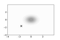
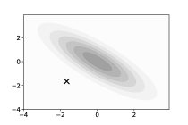
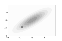
Figure 3: Assessment of calibration from $Z$-statistic and $S$-statistic. The contour plots represent the posterior distributions, and the symbol ‘$\times$’ represents the solution.
Top left: Both statistics decide that the solver is not calibrated. Top right: The $S$-statistic decides that the solver is calibrated, while the $Z$-statistic does not. Bottom: Both statistics decide that the solver is calibrated.

4.3.4 $S$-statistic for BayesCG under the Krylov prior

We show that BayesCG under the Krylov prior is not calibrated, but that it is has similar performance to a calibrated solver under full posteriors and is optimistic under approximate posteriors.

Calibration of BayesCG under full Krylov posteriors.

Theorem 2.2 implies that the $S$-statistic for any solution $\mathbf{x}_{*}$ is equal to

$$\mathrm{S}_{m}(\mathbf{x}_{*})=\|\mathbf{x}_{*}-\mathbf{x}_{m}\|_{\mathbf{A}}^{2}=\operatorname{trace}(\mathbf{A}\mathbf{\Gamma}_{m}),\qquad 1\leq m\leq g.$$

Thus, the $S$-statistic indicates that the size of Krylov posteriors is consistent with the errors, which is a desirable property of calibrated solvers. However, BayesCG under the Krylov prior is not a calibrated solver because the traces of posterior covariances from calibrated solvers are distributed around the average error instead of always being equal to the error.

Calibration of BayesCG under approximate posteriors.

From (9) follows that $\operatorname{trace}(\mathbf{A}\widehat{\mathbf{\Gamma}}_{m})$ is concentrated around smaller values than the $S$-statistic; and the underestimate of the trace is equal to the Wasserstein distance between full and approximate Krylov posteriors in Theorem 3.2. This underestimate points to the optimism of BayesCG under approximate Krylov posteriors. This optimism is expected because approximate posteriors model the uncertainty about $\mathbf{x}_{*}$ in a lower dimensional space than full posteriors.

5 Numerical experiments

We present numerical assessments of BayesCG calibration via the $Z$- and $S$-statistics.

After describing the setup of the numerical experiments (Section 5.1), we assess the calibration of three implementations of BayesCG: (i) BayesCG with random search directions (Section 5.2)—a solver known to be calibrated—so as to establish a baseline for comparisons with other versions of BayesCG; (ii) BayesCG under the inverse prior (Section 5.3); and (iii) BayesCG under the Krylov prior (Section 5.4). We choose the inverse prior and the Krylov priors because under each of these priors, the posterior mean from BayesCG coincides with the solution from CG.

Conclusions from all the experiments.

Both, $Z$- and $S$ statistics indicate that BayesCG with random search directions is indeed a calibrated solver, and that BayesCG under the inverse prior is pessimistic.

The $S$-statistic indicates that BayesCG under full Krylov posteriors mimics a calibrated solver, and that BayesCG under rank-50 approximate posteriors does as well, but not as much since it is slightly optimistic.

However, among all versions, BayesCG under approximate Krylov posteriors is the only one that is computationally practical and that is competitive with CG.

5.1 Experimental Setup

We describe the matrix $\mathbf{A}$ in the linear system (Section 5.1.1); the setup of the $Z$- and $S$-statistic experiments (Section 5.1.2); and the three BayesCG implementations (Section 5.1.3).

5.1.1 The matrix $\mathbf{A}$ in the linear system (1)

The symmetric positive definite matrix $\mathbf{A}\in\mathbb{R}^{n\times n}$ of dimension $n=1806$ is a preconditoned version of the matrix BCSSTK14 from the Harwell-Boeing collection in [1]. Specifically,

$$\mathbf{A}=\mathbf{D}^{-1/2}\mathbf{B}\mathbf{D}^{-1/2},\qquad\text{where}\quad\mathbf{D}\equiv\operatorname{diag}\begin{pmatrix}\mathbf{B}_{11}&\cdots&\mathbf{B}_{nn}\end{pmatrix}$$

and $\mathbf{B}$ is BCSSTK14. Calibration is assessed at iterations $m=10,100,300$.

5.1.2 $Z$-statistic and $S$-statistic

The $Z$-statistic and $S$-statistic experiments are implemented as described in Algorithms 3 and 4, respectively. The calibration criteria for the $Z$-statistic are given in Remark 7, and for the $S$-statistic in Remark 10.

We sample from Gaussian distributions by exploiting their stability. According to Lemma 5 in Appendix A, if $Z\sim\operatorname{\mathcal{N}}(\mathbf{0},\mathbf{I})$, and $\mathbf{F}\mathbf{F}^{T}=\mathbf{\Sigma}$ is a factorization of the covariance, then

$$\mathbf{F}Z+\mathbf{z}=X\sim\operatorname{\mathcal{N}}(\mathbf{x},\mathbf{\Sigma}).$$

Samples $Z\sim\operatorname{\mathcal{N}}(\mathbf{0},\mathbf{I})$ are generated with randn($n,1$) in Matlab, and with numpy.random.randn($n,1$) in NumPy.

$Z$-statistic experiments.

We quantify the distance between the $Z$-statistic samples and the chi-squared distribution by applying the Kolmogorov-Smirnov statistic (Definition 9) to the empirical cumulative distribution function of the $Z$-statistic samples and the analytical cumulative distribution function of the chi-squared distribution.

The degree of freedom in the chi-squared distribution is chosen as the median numerical rank of the posterior covariances. Note that the numerical rank of $\mathbf{\Sigma}_{m}$ can differ from

$$\operatorname{rank}(\mathbf{\Sigma}_{m})=\operatorname{rank}(\mathbf{\Sigma}_{0})-m,$$

and choosing the median rank gives an integer equal to the rank of at least one posterior covariance.

In compliance with the Matlab function rank and the NumPy function numpy.linalg.rank, we compute the numerical rank of $\mathbf{\Sigma}_{m}$ as

$$\operatorname{rank}(\mathbf{\Sigma}_{m})=\mathrm{cardinality}\{\sigma_{i}\ |\ \sigma_{i}>n\varepsilon\|\mathbf{\Sigma}_{m}\|_{2}\},$$ (30)

where $\varepsilon$ is machine epsilon and $\sigma_{i}$, $1\leq i\leq n$, are the singular values of $\mathbf{\Sigma}_{m}$ [15, Section 5.4.1].

5.1.3 Three BayesCG implementations

We use three versions of BayesCG: BayesCG with random search directions, BayesCG under the inverse prior, and BayesCG under the Krylov prior.

BayesCG with random search directions.

The implementation in Algorithm 6 in Appendix B.2 computes posterior covariances that do not depend on the solution $\mathbf{x}_{*}$. This, in turn, requires search directions that do not depend on $\mathbf{x}_{*}$ [7, Section 1.1] which is achieved by starting with a random search direction $\mathbf{s}_{1}=\mathbf{u}\sim\operatorname{\mathcal{N}}(\mathbf{0},\mathbf{I})$ instead of the initial residual $\mathbf{r}_{0}\equiv\mathbf{b}_{0}-\mathbf{A}\mathbf{x}_{0}$. The prior is $\operatorname{\mathcal{N}}(\mathbf{0},\mathbf{A}^{-1})$.

By design, this version of BayesCG is calibrated. However, it is also impractical due to its slow convergence, see Figure 4, and an accurate solution is available only after $n$ iterations. The random initial search direction $\mathbf{s}_{1}$ leads to uninformative $m$-dimensional subspaces, so that the solver has to explore all of $\mathbb{R}^{n}$ before finding the solution.

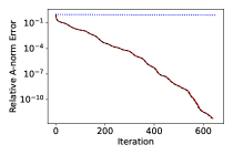
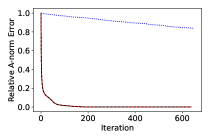
Figure 4: Relative error $\|\mathbf{x}_{*}-\mathbf{x}_{m}\|_{\mathbf{A}}^{2}/\|\mathbf{x}_{*}\|_{\mathbf{A}}^{2}$ for BayesCG under the inverse prior (solid line) and Krylov prior (dashed line), and BayesCG with random search directions (dotted line). Vertical axis has a logarithmic scale (left plot) and a linear scale (right plot).

BayesCG under the inverse prior $\mu_{0}\equiv\operatorname{\mathcal{N}}(\mathbf{0},\mathbf{A}^{-1})$.

The implementation in Algorithm 7 in Appendix B.3 is a modified version of Algorithm 1 for general priors that maintains the posterior covariances in factored form.

BayesCG under the Krylov prior.

For full posteriors, the modified Lanczos solver Algorithm 5 in Appendix B.4 computes the full prior, which is then followed by the direct computation of the posteriors from the prior in Algorithm 6.

For approximate posteriors, Algorithm 9 in Appendix B.4 computes rank-$d$ covariances at the same computational cost as $m+d$ iterations of CG.

In $Z$- and $S$-statistic experiments, solutions $\mathbf{x}_{*}$ are usually sampled from the prior distribution. We cannot sample solutions from the Krylov prior because it differs from solution to solution. Instead we sample solutions from the reference distribution $\operatorname{\mathcal{N}}(\mathbf{0},\mathbf{A}^{-1})$. This is a reasonable choice because the posterior means in BayesCG under the inverse and Krylov priors coincide with the CG iterates [8, Section 3].

5.2 BayesCG with random search directions

By design, BayesCG with random search directions is a calibrated solver. The purpose is to establish a baseline for comparisons with BayesCG under the inverse and Krylov priors, and to demonstrate that the $Z$- and $S$-statistics perform as expected on a calibrated solver.

Summary of experiments below.

Both, $Z$- and $S$-statistics strongly confirm that BayesCG with random search directions is indeed a calibrated solver, thereby corroborating the statements in Theorem 4.1 and Definition 10.

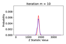
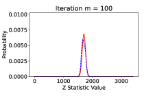
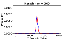
Figure 5: $Z$-statistic samples for BayesCG with random search directions after $m=10,100,300$ iterations. The solid curve represents the chi-squared distribution and the dashed curve the $Z$-statistic samples.

Iteration	$Z$-stat mean	$\chi^{2}$ mean	K-S statistic
$10.0$	$1.79\times 10^{3}$	$1.8\times 10^{3}$	$0.139$
$100.0$	$1.69\times 10^{3}$	$1.71\times 10^{3}$	$0.161$
$300.0$	$1.5\times 10^{3}$	$1.51\times 10^{3}$	$9.65\times 10^{-2}$

Table 1: This table corresponds to Figure 5. For BayesCG with random search directions, it shows the $Z$-statistic sample means; the chi-squared distribution means; and the Kolmogorov-Smirnov statistic between the $Z$-statistic samples and the chi-squared distribution.

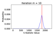
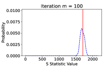
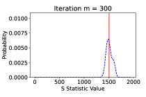
Figure 6: $S$-statistic samples and traces for BayesCG with random search directions after $m=10,100,300$ iterations. The solid curve represents the traces and the dashed curve the $S$-statistic samples.

Iteration	$S$-stat mean	Trace mean	Trace standard deviation
$10.0$	$1.78\times 10^{3}$	$1.8\times 10^{3}$	$2.93\times 10^{-12}$
$100.0$	$1.69\times 10^{3}$	$1.71\times 10^{3}$	$2.29\times 10^{-12}$
$300.0$	$1.51\times 10^{3}$	$1.51\times 10^{3}$	$2.07\times 10^{-12}$

Table 2: This table corresponds to Figure 6. For BayesCG with random search directions, it shows the $S$-statistic sample means, the trace means, and the trace standard deviations.

Figure 5 and Table 1.

The $Z$-statistic samples in Figure 5 almost match the chi-squared distribution; and the Kolmogorov-Smirnov statistics in Table 1 are on the order of $10^{-1}$, meaning close to zero. This confirms that BayesCG with random search directions is indeed calibrated.

Figure 6 and Table 2.

The traces in Figure 6 are tightly concentrated around the empirical mean of the $S$-statistic samples. Table 2 confirms the strong clustering of the trace and $S$-statistic sample means around $10^{-3}$, together with the very small deviation of the traces. Thus, the area in which the posteriors are concentrated is consistent with the error, confirming again that BayesCG with random search directions is calibrated.

5.3 BayesCG under the inverse prior $\mu_{0}=\operatorname{\mathcal{N}}(\mathbf{0},\mathbf{A}^{-1})$.

Summary of experiments below.

Both, $Z$- and $S$-statics indicate that BayesCG under the inverse prior is pessimistic, and that the pessimism increases with the iteration count. This is consistent with the experiments in [8, Section 6.1].

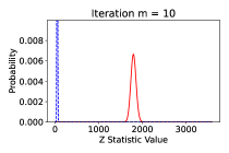
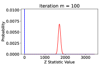
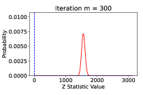
Figure 7: $Z$-statistic samples for BayesCG under the inverse prior after $m=10,100,300$ iterations. The solid curve represents the chi-squared distribution and the dashed curve the $Z$-statistic samples.

Iteration	$Z$-stat mean	$\chi^{2}$ mean	K-S statistic
$10.0$	$51.9$	$1.8\times 10^{3}$	$1.0$
$100.0$	$0.545$	$1.72\times 10^{3}$	$1.0$
$300.0$	$1.33\times 10^{-5}$	$1.56\times 10^{3}$	$1.0$

Table 3: This table corresponds to Figure 7. For BayesCG under the inverse prior, it shows the $Z$-statistic sample means; the chi-squared distribution means; and Kolmogorov-Smirnov statistic between the $Z$-statistic samples and the chi-squared and distribution.

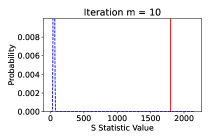
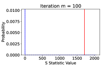
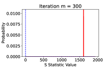
Figure 8: $S$-statistic samples and traces for BayesCG under the inverse prior after $m=10,100,300$ iterations. The solid curve represents the traces and the dashed curve the $S$-statistic samples.

Iteration	$S$-stat mean	Trace mean	Trace standard deviation
$10.0$	$51.8$	$1.8\times 10^{3}$	$2.99\times 10^{-12}$
$100.0$	$0.574$	$1.71\times 10^{3}$	$0.164$
$300.0$	$3.57\times 10^{-6}$	$1.61\times 10^{3}$	$1.02$

Table 4: This table corresponds to Figure 8. For BayesCG under the inverse prior, it shows the $S$-statistic sample means, the trace means, and the trace standard deviations.

Figure 7 and Table 3.

The $Z$-statistic samples in Figure 7 are concentrated around smaller values than the predicted chi-squared distribution. The Kol-mogorov-Smirnov statistics in Table 3 are all equal to 1, indicating no overlap between $Z$-statistic samples and chi-squared distribution. The first two columns of Table 3 show that $Z$-statistic samples move further away from the chi-squared distribution as the iterations progress. Thus, BayesCG under the inverse prior is pessimistic, and the pessimism increases with the iteration count.

Figure 8 and Table 4.

The $S$-statistic samples in Figure 8 are concentrated around smaller values than the traces. Table 4 indicates trace values at $10^{3}$, while the $S$-statistic samples move towards zero as the iteration progress. Thus the errors are much smaller than the area in which the posteriors are concentrated, meaning the posteriors overestimate the error. This again confirms the pessimism of BayesCG under the inverse prior.

5.4 BayesCG under the Krylov prior

We consider full posteriors (Section 5.4.1), and then rank-50 approximate posteriors (Section 5.4.2).

5.4.1 Full Krylov posteriors

Summary of experiments below.

The $Z$-statistic indicates that BayesCG under full Krylov posteriors is somewhat optimistic, while the $S$-statistic indicates resemblance to a calibrated solver.

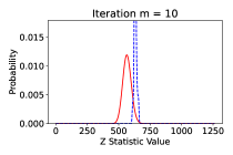
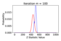
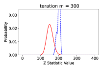
Figure 9: $Z$-statistic samples for BayesCG under the Krylov prior and full posteriors at $m=10,100,300$ iterations. The solid curve represents the predicted chi-squared distribution and the dashed curve the $Z$-statistic samples.

Iteration	$Z$-stat mean	$\chi^{2}$ mean	K-S statistic
$10.0$	$631.0$	$566.0$	$0.902$
$100.0$	$509.0$	$450.0$	$0.752$
$300.0$	$201.0$	$152.0$	$0.941$

Table 5: This table corresponds to Figure 9. For BayesCG under the Krylov prior and full posteriors, it shows the $Z$-statistic sample means; the chi-squared distribution means; and the Kolmogorov-Smirnov statistic between the $Z$-statistic samples and the chi-squared distribution.

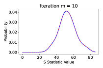
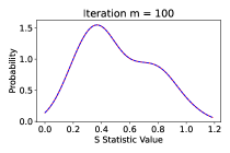
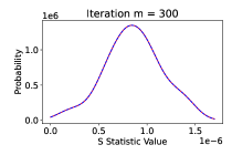
Figure 10: $S$-statistic samples and traces for BayesCG under the Krylov prior and full posteriors at $m=10,100,300$ iterations. The solid curve represents the traces and the dashed curve the $S$-statistic samples.

Iteration	$S$-stat mean	Trace mean	Trace standard deviation
$10.0$	$52.9$	$52.9$	$9.4$
$100.0$	$0.515$	$0.515$	$0.241$
$300.0$	$8.59\times 10^{-7}$	$8.59\times 10^{-7}$	$2.84\times 10^{-7}$

Table 6: This table corresponds to Figure 10. For BayesCG under the Krylov prior and full posteriors, it shows the $S$-statistic sample means, the trace means, and the trace standard deviations.

Figure 9 and Table 5.

The $Z$-statistic samples in Figure 9 are concentrated at somewhat larger values than the predicted chi-squared distribution. The Kolmogorov-Smirnov statistics in Table 5 are around .8 and .9, thus close to 1, and indicate very little overlap between $Z$-statistic samples and chi-squared distribution. Thus, BayesCG under full Krylov posteriors is somewhat optimistic.

These numerical results differ from Theorem 4.2, which predicts $Z$-statistic samples equal to $g-m$. A possible reason might be that the rank of the Krylov prior computed by Algorithm 5 is smaller than the exact rank. In exact arithmetic, $\operatorname{rank}(\mathbf{\Gamma}_{0})=g=n=1806$. However, in finite precision, $\operatorname{rank}(\mathbf{\Gamma}_{0})$ is determined by the convergence tolerance which is set to $10^{-12}$, resulting in $\operatorname{rank}(\mathbf{\Gamma}_{0})<g$.

Figure 10 and Table 6.

The $S$-statistic samples in Figure 10 match the traces extremely well, with Table 6 showing an agreement to 3 figures, as predicted in Section 4.3.4, Thus, the area in which the posteriors are concentrated is consistent with the error, as would be expected from a calibrated solver.

However, BayesCG under the Krylov prior does not behave exactly like a calibrated solver, such as BayesCG with random search directions in Section 5.2, where all traces are concentrated at the empirical mean of the $S$-statistic samples. Thus, BayesCG under the Krylov prior is not calibrated but has a performance similar to that of a calibrated solver.

5.4.2 Rank-50 approximate Krylov posteriors

Summary of the experiments below.

Both, $Z$- and $S$-statistic indicate that BayesCG under rank-50 approximate Krylov posteriors is somewhat optimistic, and is not as close to a calibrated solver as BayesCG with full Krylov posteriors. In contrast to the $Z$-statistic, the respective $S$-statistic samples and traces for BayesCG under full and rank-50 posteriors are close.

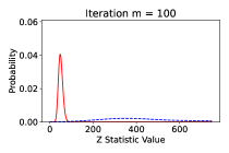
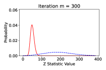
Figure 11: $Z$-statistic samples for BayesCG under rank-50 approximate Krylov posteriors at $m=10,100,300$ iterations. The solid curve represents the predicted chi-squared distribution and the dashed curve the $Z$-statistic samples.

Iteration	$Z$-stat mean	$\chi^{2}$ mean	K-S statistic
$10.0$	$319.0$	$50.0$	$1.0$
$100.0$	$375.0$	$50.0$	$1.0$
$300.0$	$194.0$	$50.0$	$1.0$

Table 7: This table corresponds to Figure 11. For BayesCG under rank-50 approximate Krylov posteriors, it shows the $Z$-statistic sample means; chi-squared distribution means; and Kolmogorov-Smirnov statistic between the $Z$-statistic samples and the chi-squared distribution.

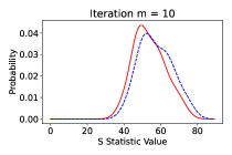
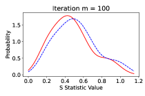
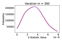
Figure 12: $S$-statistic samples and traces for BayesCG under rank-50 approximate Krylov posteriors at $m=10,100,300$ iterations. The solid curve represents the traces and the dashed curve the $S$-statistic samples.

Iteration	$S$-stat mean	Trace mean	Trace standard deviation
$10.0$	$57.2$	$53.9$	$8.32$
$100.0$	$0.517$	$0.467$	$0.214$
$300.0$	$3.37\times 10^{-6}$	$3.29\times 10^{-6}$	$1.6\times 10^{-6}$

Table 8: This table corresponds to Figure 12. For BayesCG under rank-50 approximate Krylov posteriors, it shows the $S$-statistic sample means, trace means, and trace standard deviations.

Figure 11 and Table 7.

The $Z$-statistic samples in Figure 11 are concentrated around larger values than the predicted chi-squared distribution, which is steady at 50. All Kolmogorov-Smirnov statistics in Table 7 are equal to 1, indicating no overlap between $Z$-statistic samples and chi-squared distribution. Thus, BayesCG under approximate Krylov posteriors is more optimistic than BayesCG under full posteriors.

Figure 12 and Table 8.

The traces in Figure 12 are concentrated around slightly smaller values than the $S$-statistic samples, but they all have the same order of magnitude, as shown in Table 8. This means, the errors are slightly larger than the area in which the posteriors are concentrated; and the posteriors slightly underestimate the errors.

A comparison of Tables 6 and 8 shows that the $S$-statistic samples and traces, respectively, for full and rank-50 posteriors are close. From the point of view of the $S$-statistic, BayesCG under approximate Krylov posteriors is somewhat optimistic, and close to being a calibrated solver but not as close as BayesCG under full Krylov posteriors.

Appendix A Auxiliary Results

We present auxiliary results required for proofs in other sections.

The stability of Gaussian distributions implies that a linear transformation of a Gaussian random variable remains Gaussian.

Lemma 5 (Stability of Gaussian Distributions [27, Section 1.2])

Let $X\sim\operatorname{\mathcal{N}}(\mathbf{x},\mathbf{\Sigma})$ be a Gaussian random variable with mean $\mathbf{x}\in\mathbb{R}^{n}$ and covariance $\mathbf{\Sigma}\in\mathbb{R}^{n\times n}$. If $\mathbf{y}\in\mathbb{R}^{n}$ and $\mathbf{F}\in\mathbb{R}^{n\times n}$, then

$$Z=\mathbf{y}+\mathbf{F}X\sim\operatorname{\mathcal{N}}(\mathbf{y}+\mathbf{F}\mathbf{x},\mathbf{F}\mathbf{\Sigma}\mathbf{F}^{T}).$$

The conjugacy of Gaussian distributions implies that the distribution of a Gaussian random variable conditioned on information that linearly depends on the random variable is a Gaussian distribution.

Lemma 6 (Conjugacy of Gaussian Distributions [30, Section 6.1], [37, Corollary 6.21])

Let $X\sim\operatorname{\mathcal{N}}(\mathbf{x},\mathbf{\Sigma}_{x})$ and $Y\sim\operatorname{\mathcal{N}}(\mathbf{y},\mathbf{\Sigma}_{y})$. The jointly Gaussian random variable $\begin{bmatrix}X^{T}&Y^{T}\end{bmatrix}^{T}$ has the distribution

$$\begin{bmatrix}X\\ Y\end{bmatrix}\sim\operatorname{\mathcal{N}}\left(\begin{bmatrix}\mathbf{x}\\ \mathbf{y}\end{bmatrix},\begin{bmatrix}\mathbf{\Sigma}_{x}&\mathbf{\Sigma}_{xy}\\ \mathbf{\Sigma}_{xy}^{T}&\mathbf{\Sigma}_{y}\end{bmatrix}\right),$$

where $\mathbf{\Sigma}_{xy}\equiv\operatorname{Cov}(X,Y)=\operatorname{\mathbb{E}}[(X-\mathbf{x})(Y-\mathbf{y})^{T}]$ and the conditional distribution of $X$ given $Y$ is

$$(X\ |\ Y)\sim\operatorname{\mathcal{N}}(\overbrace{\mathbf{x}+\mathbf{\Sigma}_{xy}\mathbf{\Sigma}_{y}^{\dagger}(Y-\mathbf{y})}^{\text{mean}},\ \overbrace{\mathbf{\Sigma}_{x}-\mathbf{\Sigma}_{xy}\mathbf{\Sigma}_{y}^{\dagger}\mathbf{\Sigma}_{xy}^{T}}^{\text{covariance}}).$$

We show how to transform a $\mathbf{B}$-orthogonal matrix into an orthogonal matrix.

Lemma 7

Let $\mathbf{B}\in\mathbb{R}^{n\times n}$ be symmetric positive definite, and let $\mathbf{H}\in\mathbb{R}^{n\times n}$ be a $\mathbf{B}$-orthogonal matrix with $\mathbf{H}^{T}\mathbf{B}\mathbf{H}=\mathbf{H}\mathbf{B}\mathbf{H}^{T}=\mathbf{I}$. Then

$$\mathbf{U}\equiv\mathbf{B}^{1/2}\mathbf{H}$$

is an orthogonal matrix with $\mathbf{U}^{T}\mathbf{U}=\mathbf{U}\mathbf{U}^{T}=\mathbf{I}$.

Proof

The symmetry of $\mathbf{B}$ and the $\mathbf{B}$-orthogonality of $\mathbf{H}$ imply

$$\mathbf{U}^{T}\mathbf{U}=\mathbf{H}^{T}\mathbf{B}\mathbf{H}=\mathbf{I}.$$

From the orthonormality of the columns of $\mathbf{U}$, and the fact that $\mathbf{U}$ is square follows that $\mathbf{U}$ is an orthogonal matrix [21, Definition 2.1.3]. ∎

Definition 11

[21, Section 7.3] The thin singular value decomposition of the rank-$p$ matrix $\mathbf{G}\in\mathbb{R}^{m\times n}$ is

$$\mathbf{G}=\mathbf{U}\mathbf{D}\mathbf{W}^{T},$$

where $\mathbf{U}\in\mathbb{R}^{m\times p}$ and $\mathbf{W}\in\mathbb{R}^{n\times p}$ are matrices with orthonormal columns and $\mathbf{D}\in\mathbb{R}^{p\times p}$ is a diagonal matrix with positive diagonal elements. The Moore-Penrose inverse of $\mathbf{G}$ is

$$\mathbf{G}^{\dagger}=\mathbf{W}\mathbf{D}^{-1}\mathbf{U}^{T}.$$

If a matrix has full column-rank or full row-rank, then its Moore-Penrose can be expressed in terms of the matrix itself. Furthermore, the Moore-Penrose inverse of a product is equal to the product of the Moore-Penrose inverses, provided the first matrix has full column-rank and the second matrix has full row-rank.

Lemma 8 ([5, Corollary 1.4.2])

Let $\mathbf{G}\in\mathbb{R}^{m\times n}$ and $\mathbf{J}\in\mathbb{R}^{n\times p}$ have full column and row rank respectively, so $\operatorname{rank}(\mathbf{G})=\operatorname{rank}(\mathbf{J})=n$. The Moore-Penrose inverses of $\mathbf{G}$ and $\mathbf{J}$ are

$$\mathbf{G}^{\dagger}=(\mathbf{G}^{T}\mathbf{G})^{-1}\mathbf{G}^{T}\quad\text{and}\quad\mathbf{J}^{\dagger}=\mathbf{J}^{T}(\mathbf{J}\mathbf{J}^{T})^{-1}$$

respectively, and the Moore-Penrose inverse of the product equals

$$(\mathbf{G}\mathbf{J})^{\dagger}=\mathbf{J}^{\dagger}\mathbf{G}^{\dagger}.$$

Below is an explicit expression for the mean of a quadratic form of Gaussians.

Lemma 9 ([26, Sections 3.2b.1–3.2b.3])

Let $Z\sim\operatorname{\mathcal{N}}(\mathbf{x}_{z},\mathbf{\Sigma}_{z})$ be a Gaussian random variable in $\mathbb{R}^{n}$, and $\mathbf{B}\in\mathbb{R}^{n\times n}$ be symmetric positive definite. The mean of $Z^{T}\mathbf{B}Z$ is

$$\operatorname{\mathbb{E}}[Z^{T}\mathbf{B}Z] =\operatorname{trace}(\mathbf{B}\mathbf{\Sigma}_{z})+\mathbf{x}_{z}^{T}\mathbf{B}\mathbf{x}_{z}.$$

We show that the squared Euclidean norm of a Gaussian random variable with an orthogonal projector as its covariance matrix is distributed according to a chi-squared distribution.

Lemma 10

Let $Z\sim\operatorname{\mathcal{N}}(\mathbf{0},\mathbf{P})$ be a Gaussian random variable in $\mathbb{R}^{n}$. If the covariance matrix $\mathbf{P}$ is an orthogonal projector, that is, if $\mathbf{P}^{2}=\mathbf{P}$ and $\mathbf{P}=\mathbf{P}^{T}$, then

$$\|X\|_{2}^{2}=(X^{T}X)\sim\chi_{p}^{2},$$

where $p=\operatorname{rank}(\mathbf{P})$.

Proof

We express the projector in terms of orthonormal matrices and then use the invariance of the 2-norm under orthogonal matrices and the stability of Gaussians.

Since $\mathbf{P}$ is an orthogonal projector, there exists $\mathbf{U}_{1}\in\mathbb{R}^{n\times p}$ such that $\mathbf{U}_{1}\mathbf{U}_{1}^{T}=\mathbf{P}$ and $\mathbf{U}_{1}^{T}\mathbf{U}=\mathbf{I}_{p}$. Choose $\mathbf{U}_{2}\in\mathbb{R}^{n\times(n-p)}$ so that $\mathbf{U}=\begin{bmatrix}\mathbf{U}_{1}&\mathbf{U}_{2}\end{bmatrix}$ is an orthogonal matrix. Thus,

$$X^{T}X=X^{T}\mathbf{U}\mathbf{U}^{T}X=X^{T}\mathbf{U}_{1}\mathbf{U}_{1}^{T}X+X^{T}\mathbf{U}_{2}\mathbf{U}_{2}^{T}X.$$ (31)

Lemma 5 implies that $Y=\mathbf{U}_{1}^{T}X$ is distributed according to a Gaussian distribution with mean $\mathbf{0}$ and covariance $\mathbf{U}_{1}^{T}\mathbf{U}_{1}\mathbf{U}_{1}^{T}\mathbf{U}=\mathbf{I}_{p}$. Similarly, $Z=\mathbf{U}_{2}^{T}X$ is distributed according to a Gaussian distribution with mean $\mathbf{0}$ and covariance $\mathbf{U}_{2}^{T}\mathbf{U}_{1}\mathbf{U}_{1}^{T}\mathbf{U}_{2}=\mathbf{0}$, thus $Z=\mathbf{0}$.

Substituting $Y$ and $Z$ into (31) gives $X^{T}X=Y^{T}Y+\mathbf{0}^{T}\mathbf{0}$. From $Y\sim\operatorname{\mathcal{N}}(\mathbf{0},\mathbf{I}_{p})$ follows $(X^{T}X)\sim\chi_{p}^{2}$. ∎

Lemma 11

If $\mathbf{A}\in\mathbb{R}^{n\times n}$ is symmetric positive definite, and $M\sim\operatorname{\mathcal{N}}(\mathbf{x}_{\mu}\mathbf{\Sigma}_{\mu})$ and $N\sim\operatorname{\mathcal{N}}(\mathbf{x}_{\nu},\mathbf{\Sigma}_{\nu})$ are independent random variables in $\mathbb{R}^{n}$, then

$$\operatorname{\mathbb{E}}[\|M-N\|_{\mathbf{A}}^{2}]=\|\mathbf{x}_{\mu}-\mathbf{x}_{\nu}\|_{\mathbf{A}}^{2}+\operatorname{trace}(\mathbf{A}\mathbf{\Sigma}_{\mu})+\operatorname{trace}(\mathbf{A}\mathbf{\Sigma}_{\nu}).$$

Proof

The random variable $M-N$ has mean $\operatorname{\mathbb{E}}[M-N]=\mathbf{x}_{\mu}-\mathbf{x}_{\nu}$, and covariance

$$\mathbf{\Sigma}_{M-N} \equiv\operatorname{Cov}(M-N,M-N)$$

$$=\operatorname{Cov}(M,M)+\operatorname{Cov}(N,N)-\operatorname{Cov}(M,N)-\operatorname{Cov}(N,M)$$

$$=\operatorname{Cov}(M,M)+\operatorname{Cov}(N,N)=\mathbf{\Sigma}_{\mu}+\mathbf{\Sigma}_{\nu},$$

where the covariances $\operatorname{Cov}(M,N)=\operatorname{Cov}(N,M)=0$ because $M$ and $N$ are independent. Now apply Lemma 9 to $M-N$. ∎

Appendix B Algorithms

We present algorithms for the modified Lanczos method (Section B.1), BayesCG with random search directions (Section B.2), BayesCG with covariances in factored form (Section B.3), and BayesCG under the Krylov prior (Section B.4).

B.1 Modified Lanczos method

The Lanczos method [34, Algorithm 6.15] produces an orthonormal basis for the Krylov space $\mathcal{K}_{g}(\mathbf{A},\mathbf{v}_{1})$, while the modified version in Algorithm 5 produces an $\mathbf{A}$-orthonormal basis.

Algorithm 5 Modified Lanczos Method

1:Input: spd $\mathbf{A}\in\mathbb{R}^{n\times n}$, $\mathbf{v}_{1}\in\mathbb{R}^{n}$, basis dimension $m$, convergence tolerance $\varepsilon$

2:$\mathbf{v}_{0}=\mathbf{0}\in\mathbb{R}^{n}$

3:$i=1$

4:$\beta=(\mathbf{v}_{i}^{T}\mathbf{A}\mathbf{v}_{i})^{1/2}$

5:$\mathbf{v}_{i}=\mathbf{v}_{i}/\beta$

6:while  $i\leq m$ do

7:     $\mathbf{w}=\mathbf{A}\mathbf{v}_{i}-\beta\mathbf{v}_{i-1}$

8:     $\alpha=\mathbf{w}^{T}\mathbf{A}\mathbf{v}_{i}$

9:     $\mathbf{w}=w-\alpha\mathbf{v}_{i}$

10:     $\mathbf{w}=\mathbf{w}-\sum_{j=1}^{i}\mathbf{v}_{j}\mathbf{v}_{j}^{T}\mathbf{A}\mathbf{w}$ $\triangleright$ Reorthogonalize $\mathbf{w}$

11:     $\mathbf{w}=\mathbf{w}-\sum_{j=1}^{i}\mathbf{v}_{j}\mathbf{v}_{j}^{T}\mathbf{A}\mathbf{w}$

12:     $\beta=(\mathbf{w}^{T}\mathbf{A}\mathbf{w})^{1/2}$

13:     if  $\beta<\varepsilon$ then

14:         Exit while loop

15:     end if

16:     $i=i+1$

17:     $\mathbf{v}_{i}=\mathbf{w}/\beta$

18:end while

19:$m=i-1$ $\triangleright$ Number of basis vectors

20:Output: $\{\mathbf{v}_{1},\mathbf{v}_{2},\ldots,\mathbf{v}_{m}\}$$\triangleright$ $\mathbf{A}$-orthonormal basis of $\mathcal{K}_{m}(\mathbf{A},\mathbf{v}_{1})$

Algorithm 5 reorthogonalizes the basis vectors $\mathbf{v}_{i}$ with Classical Gram-Schmidt performed twice, see Lines 10 and 11. This reorthogonalization technique can be implemented efficiently and produces vectors that are orthogonal to machine precision [13, 14].

B.2 BayesCG with random search directions

The version of BayesCG in Algorithm 6 is designed to be calibrated because the search directions do not depend on $\mathbf{x}_{*}$, hence the posteriors do not depend on $\mathbf{x}_{*}$ either [7, Section 1.1].

After sampling an initial random search direction $\mathbf{s}_{1}\sim\operatorname{\mathcal{N}}(\mathbf{0},\mathbf{I})$, Algorithm 6 computes an $\mathbf{A}\mathbf{\Sigma}_{0}\mathbf{A}$-orthonormal basis for the Krylov space $\mathcal{K}_{m}(\mathbf{A}\mathbf{\Sigma}_{0}\mathbf{A},\mathbf{s}_{1})$ with Algorithm 5. Then Algorithm 6 computes the BayesCG posteriors directly with (2) and (3) from Theorem 2.1. The numerical experiments in Section 5 run Algorithm 6 with the inverse prior $\mu_{0}=\operatorname{\mathcal{N}}(\mathbf{0},\mathbf{A}^{-1})$.

Algorithm 6 BayesCG with random search directions

1:Inputs: spd $\mathbf{A}\in\mathbb{R}^{n\times n}$, $\mathbf{b}\in\mathbb{R}^{n}$, prior $\mu_{0}=\operatorname{\mathcal{N}}(\mathbf{x}_{0},\mathbf{\Sigma}_{0})$, iteration count $m$

2:${\mathbf{r}}_{0}={\mathbf{b}}-{\mathbf{A}\mathbf{x}}_{0}$ $\triangleright$ Initial residual

3:Sample $\mathbf{s}_{1}$ from $\operatorname{\mathcal{N}}(\mathbf{0},\mathbf{I})$ $\triangleright$ Initial search direction

4:Compute columns of $\mathbf{S}$ with Algorithm 5

5:$\mathbf{\Lambda}_{m}=\mathbf{S}_{m}^{T}\mathbf{A}\mathbf{\Sigma}_{0}\mathbf{A}\mathbf{S}_{m}$ $\triangleright$ $\mathbf{\Lambda}_{m}$ is diagonal

6:$\mathbf{x}_{m}=\mathbf{x}_{0}+\mathbf{\Sigma}_{0}\mathbf{A}\mathbf{S}_{m}\mathbf{\Lambda}_{m}^{-1}\mathbf{S}_{m}^{T}\mathbf{r}_{0}$ $\triangleright$ Compute posterior mean with (2)

7:$\mathbf{\Sigma}_{m}=\mathbf{\Sigma}_{0}-\mathbf{\Sigma}_{0}\mathbf{A}\mathbf{S}_{m}\mathbf{\Lambda}_{m}^{-1}\mathbf{S}_{m}^{T}\mathbf{A}\mathbf{\Sigma}_{0}$ $\triangleright$ Compute posterior covariance with (3)

8:Output: $\mu_{m}=\mathcal{N}(\mathbf{x}_{m},\mathbf{\Sigma}_{m})$

B.3 BayesCG with covariances in factored form

Algorithm 7 takes as input a general prior covariance $\mathbf{\Sigma}_{0}$ in factored form, and subsequently maintains the posterior covariances $\mathbf{\Sigma}_{m}$ in factored form as well. Theorem B.1 presents the correctness proof for Algorithm 7.

Theorem B.1

Under the conditions of Theorem 2.1, if $\mathbf{\Sigma}_{0}=\mathbf{F}_{0}\mathbf{F}_{0}^{T}$ for $\mathbf{F}_{0}\in\mathbb{R}^{n\times\ell}$ and some $m\leq\ell\leq n$, then $\mathbf{\Sigma}_{m}=\mathbf{F}_{m}\mathbf{F}_{m}^{T}$ with

$$\mathbf{F}_{m}=\mathbf{F}_{0}\left(\mathbf{I}-\mathbf{F}_{0}^{T}\mathbf{A}\mathbf{S}_{m}(\mathbf{S}_{m}^{T}\mathbf{A}\mathbf{F}_{0}\mathbf{F}_{0}^{T}\mathbf{A}\mathbf{S}_{m})^{-1}\mathbf{S}_{m}\mathbf{A}\mathbf{F}_{0}\right)\in\mathbb{R}^{n\times\ell},\qquad 1\leq m\leq n.$$

Proof

Fix $m$. Substituting $\mathbf{\Sigma}_{0}=\mathbf{F}_{0}\mathbf{F}_{0}^{T}$ into (3) and factoring out $\mathbf{F}_{0}$ on the left and $\mathbf{F}_{0}^{T}$ on the right gives $\mathbf{\Sigma}_{m}=\mathbf{F}_{0}\mathbf{P}\mathbf{F}_{0}^{T}$ where

$$\mathbf{P} \equiv\mathbf{I}-\mathbf{F}_{0}^{T}\mathbf{A}\mathbf{S}_{m}(\mathbf{S}_{m}^{T}\mathbf{A}\mathbf{F}_{0}\mathbf{F}_{0}^{T}\mathbf{A}\mathbf{S}_{m})^{-1}\mathbf{S}_{m}\mathbf{A}\mathbf{F}_{0}$$

$$=(\mathbf{I}-\mathbf{Q}(\mathbf{Q}^{T}\mathbf{Q})^{-1}\mathbf{Q}^{T})\qquad\text{where}\quad\mathbf{Q}\equiv\mathbf{F}_{0}^{T}\mathbf{A}\mathbf{S}_{m}.$$

Show that $\mathbf{P}$ is a projector,

$$\mathbf{P}^{2} =\mathbf{I}-2\mathbf{Q}(\mathbf{Q}^{T}\mathbf{Q})^{-1}\mathbf{Q}^{T}+\mathbf{Q}(\mathbf{Q}^{T}\mathbf{Q})^{-1}\mathbf{Q}^{T}\mathbf{Q}(\mathbf{Q}^{T}\mathbf{Q})^{-1}\mathbf{Q}^{T}$$

$$=\mathbf{I}-\mathbf{Q}(\mathbf{Q}^{T}\mathbf{Q})^{-1}\mathbf{Q}^{T}=\mathbf{P}.$$

Hence $\mathbf{\Sigma}_{m}=\mathbf{F}_{0}\mathbf{P}\mathbf{F}_{0}^{T}=\mathbf{F}_{0}\mathbf{P}\mathbf{P}\mathbf{F}_{0}^{T}=\mathbf{F}_{m}\mathbf{F}_{m}^{T}$.

Algorithm 7 BayesCG with covariances in factored form

1:Input: spd $\mathbf{A}\in\mathbb{R}^{n\times n}$, $\mathbf{b}\in\mathbb{R}^{n}$, $\mathbf{x}_{0}\in\mathbb{R}^{n}$, $\mathbf{F}_{0}\in\mathbb{R}^{n\times\ell}$ $\triangleright$ need $\mathbf{x}_{*}-\mathbf{x}_{0}\in\operatorname{range}(\mathbf{\Sigma}_{0})$

2:$\mathbf{r}_{0}=\mathbf{b}-\mathbf{A}\mathbf{x}_{0}$

3:$\mathbf{s}_{1}=\mathbf{r}_{0}$

4:$\mathbf{P}=\mathbf{0}\in\mathbb{R}^{n\times n}$

5:$m=0$

6:while not converged do

7:     $m=m+1$

8:     $\mathbf{P}(:,m)=\mathbf{F}_{0}^{T}\mathbf{A}\mathbf{s}_{m}$ $\triangleright$ Save column $m$ of $\mathbf{P}$

9:     $\mathbf{q}=\mathbf{F}_{0}\mathbf{P}(:,m)$ $\triangleright$ Compute $\mathbf{q}=\mathbf{\Sigma}_{0}\mathbf{A}\mathbf{s}_{m}$

10:     $\eta_{m}=\mathbf{s}_{m}^{T}\mathbf{A}\mathbf{q}$

11:     $\mathbf{P}(:,m)=\mathbf{P}(:,m)\big{/}\eta_{m}$ $\triangleright$ Normalize column $m$ of $\mathbf{P}$

12:     $\alpha_{m}=\left(\mathbf{r}_{m-1}^{T}\mathbf{r}_{m-1}\right)\big{/}\eta_{m}$

13:     $\mathbf{x}_{m}=\mathbf{x}_{m-1}+\alpha_{m}\mathbf{q}$

14:     $\mathbf{r}_{m}=\mathbf{r}_{m-1}-\alpha_{m}\mathbf{A}\mathbf{q}$

15:     $\beta_{m}=\left(\mathbf{r}_{m}^{T}\mathbf{r}_{m}\right)\big{/}\left(\mathbf{r}_{m-1}^{T}\mathbf{r}_{m-1}\right)$

16:     $\mathbf{s}_{m+1}=\mathbf{r}_{m}+\beta_{m}\mathbf{s}_{m}$

17:end while

18:$\mathbf{P}=\mathbf{P}(:,1:m)$ $\triangleright$ Discard unused columns of $\mathbf{P}$

19:$\mathbf{F}_{m}=\mathbf{F}_{0}(\mathbf{I}-\mathbf{P}\mathbf{P}^{T})$

20:Output: $\mathbf{x}_{m}$, $\mathbf{F}_{m}$ $\triangleright$ Final posterior

B.4 BayesCG under the Krylov prior

We present algorithms for BayesCG under full Krylov posteriors (Section B.4.1) and under approximate Krylov posteriors (Section B.4.2).

B.4.1 Full Krylov posteriors

Algorithm 8 computes the following: a matrix $\mathbf{V}$ whose columns are an $\mathbf{A}$-orthonormal basis for $\mathcal{K}_{g}(\mathbf{A},\mathbf{r}_{0})$; the diagonal matrix $\mathbf{\Phi}$ in (5); and the posterior mean $\mathbf{x}_{m}$ in (26). The output consists of the posterior mean $\mathbf{x}_{m}$, and the factors $\mathbf{V}_{m+1:g}$ and $\mathbf{\Phi}_{m+1:g}$ for the posterior covariance.

Algorithm 8 BayesCG under the Krylov prior with full posteriors

1:Inputs: spd $\mathbf{A}\in\mathbb{R}^{n\times n}$, $\mathbf{b}\in\mathbb{R}^{n}$, $\mathbf{x}_{0}\in\mathbb{R}^{n}$, iteration count $m$

2:${\mathbf{r}}_{0}={\mathbf{b}}-{\mathbf{A}\mathbf{x}}_{0}$ $\triangleright$ Initial residual

3:${\mathbf{v}}_{1}={\mathbf{r}}_{0}$ $\triangleright$ Initial search direction

4:Compute columns of $\mathbf{V}$ with Algorithm 5

5:$\mathbf{\Phi}=\mathrm{diag}((\mathbf{V}^{T}\mathbf{r}_{0})^{2})$ $\triangleright$ Compute $\mathbf{\Phi}$ with (5)

6:$\mathbf{x}_{m}=\mathbf{x}_{0}+\mathbf{V}_{1:m}\mathbf{V}_{1:m}^{T}\mathbf{r}_{0}$ $\triangleright$ Compute posterior mean with (26)

7:Output: $\mathbf{x}_{m}$, $\mathbf{V}_{m+1:g}$, $\mathbf{\Phi}_{m+1:g}$

B.4.2 Approximate Krylov posteriors

Algorithm 9 computes rank-$d$ approximate Krylov posteriors in two main steps: (i) posterior mean and iterates $\mathbf{x}_{m}$ in Lines 5-14; and (ii) factorization of the posterior covariance $\widehat{\mathbf{\Gamma}}_{m}$ in Lines 16-26.

Algorithm 9 BayesCG under the Krylov prior [32, Algorithm 3.1]

1:Inputs: spd $\mathbf{A}\in\mathbb{R}^{n\times n}$, $\mathbf{b}\in\mathbb{R}^{n}$, $\mathbf{x}_{0}\in\mathbb{R}^{n}$, iteration count $m$, posterior rank $d$

2:${\mathbf{r}}_{0}={\mathbf{b}}-{\mathbf{A}\mathbf{x}}_{0}$ $\triangleright$ Initial residual

3:${\mathbf{v}}_{1}={\mathbf{r}}_{0}$ $\triangleright$ Initial search direction

4:$i=0$ $\triangleright$ Initial iteration counter

5:while $i<m$ do $\triangleright$ CG recursions for posterior means

6:     $i=i+1$ $\triangleright$ Increment iteration count

7:     $\eta_{i}=\mathbf{v}_{i}^{T}\mathbf{A}\mathbf{v}_{i}$

8:     $\gamma_{i}=(\mathbf{r}_{i-1}^{T}\mathbf{r}_{i-1})\big{/}\eta_{i}$ $\triangleright$ Next step size

9:     ${\mathbf{x}}_{i}={\mathbf{x}}_{i-1}+\gamma_{i}\mathbf{v}_{i}$ $\triangleright$ Next iterate

10:     ${\mathbf{r}}_{i}={\mathbf{r}}_{i-1}-\gamma_{i}\mathbf{A}\mathbf{v}_{i}$ $\triangleright$ Next residual

11:     $\delta_{i}=(\mathbf{r}_{i}^{T}\mathbf{r}_{i})\big{/}(\mathbf{r}_{i-1}^{T}\mathbf{r}_{i-1})$

12:     $\mathbf{v}_{i+1}=\mathbf{r}_{i}+\delta_{i}\mathbf{v}_{i}$ $\triangleright$ Next search direction

13:end while

14:$d=\min\{d,g-m\}$ $\triangleright$ Compute full rank posterior if $d>g-m$

15:$\mathbf{V}_{m+1:m+d}=\mathbf{0}_{n\times d}$ $\triangleright$ Initialize approximate posterior matrices

16:$\mathbf{\Phi}_{m+1:m+d}=\mathbf{0}_{d\times d}$

17:for $j=m+1:m+d$ do $\triangleright$ $d$ additional iterations for posterior covariance

18:     $\eta_{j}=\mathbf{v}_{j}^{T}\mathbf{A}\mathbf{v}_{j}$

19:     $\gamma_{j}=(\mathbf{r}_{j-1}^{T}\mathbf{r}_{j-1})\big{/}\eta_{j}$

20:     $\mathbf{V}(:,j)=\mathbf{v}_{j}\big{/}\sqrt{\eta_{j}}$ $\triangleright$ Next column of $\mathbf{V}_{m+1,m+d}$

21:     $\mathbf{\Phi}(j,j)=\gamma_{j}\|\mathbf{r}_{j-1}\|_{2}^{2}$ $\triangleright$ Next diagonal element of $\mathbf{\Phi}_{m+1,m+d}$

22:     $\mathbf{r}_{j}=\mathbf{r}_{j-1}-\gamma_{j}\mathbf{A}\mathbf{v}_{j}$

23:     $\delta_{j}=(\mathbf{r}_{j}^{T}\mathbf{r}_{j})\big{/}(\mathbf{r}_{j-1}^{T}\mathbf{r}_{j-1})$

24:     $\mathbf{v}_{j+1}=\mathbf{r}_{j}+\delta_{j}\mathbf{v}_{j}$ $\triangleright$ Next un-normalized column of $\mathbf{V}_{m+1,m+d}$

25:end for

26:Output: $\mathbf{x}_{m}$, $\mathbf{V}_{m+1:m+d}$, $\mathbf{\Phi}_{m+1:m+d}$

References

• [1] BCSSTK14: BCS Structural Engineering Matrices (linear equations) Roof of the Omni Coliseum, Atlanta.
• [2] S. Bartels, J. Cockayne, I. C. F. Ipsen, and P. Hennig. Probabilistic linear solvers: a unifying view. Stat. Comput., 29(6):1249–1263, 2019.
• [3] J. O. Berger. Statistical Decision Theory and Bayesian Analysis. Springer New York, 1985.
• [4] M. Berljafa and S. Güttel. Generalized rational Krylov decompositions with an application to rational approximation. SIAM J. Matrix Anal. Appl., 36(2):894–916, 2015.
• [5] S. L. Campbell and C. D. Meyer. Generalized inverses of linear transformations, volume 56 of Classics in Applied Mathematics. Society for Industrial and Applied Mathematics (SIAM), Philadelphia, PA, 2009.
• [6] J. Cockayne, M. M. Graham, C. J. Oates, and T. J. Sullivan. Testing whether a learning procedure is calibrated, 2021. arXiv:2012.12670.
• [7] J. Cockayne, I. C. F. Ipsen, C. J. Oates, and T. W. Reid. Probabilistic iterative methods for linear systems. J. Mach. Learn. Res., 22 (232):1–34, 2021.
• [8] J. Cockayne, C. J. Oates, I. C. F. Ipsen, and M. Girolami. A Bayesian conjugate gradient method (with discussion). Bayesian Anal., 14(3):937–1012, 2019. Includes 6 discussions and a rejoinder from the authors.
• [9] J. Cockayne, C. J. Oates, I. C. F. Ipsen, and M. Girolami. Supplementary material for ‘A Bayesian conjugate-gradient method’. Bayesian Anal., 2019.
• [10] J. Cockayne, C. J. Oates, T. J. Sullivan, and M. Girolami. Bayesian probabilistic numerical methods. SIAM Rev., 61(4):756–789, 2019.
• [11] Vladimir Fanaskov. Uncertainty calibration for probabilistic projection methods. Stat. Comput., 31(5):Paper No. 56, 17, 2021.
• [12] M. Gelbrich. On a formula for the $L^{2}$ Wasserstein metric between measures on Euclidean and Hilbert spaces. Math. Nachr., 147:185–203, 1990.
• [13] L. Giraud, J. Langou, and M. Rozloznik. The loss of orthogonality in the Gram-Schmidt orthogonalization process. Comput. Math. Appl., 50(7):1069–1075, 2005.
• [14] Luc Giraud, Julien Langou, Miroslav Rozložník, and Jasper van den Eshof. Rounding error analysis of the classical Gram-Schmidt orthogonalization process. Numer. Math., 101(1):87–100, 2005.
• [15] Gene H. Golub and Charles F. Van Loan. Matrix Computations. The Johns Hopkins University Press, Baltimore, 4th edition, 2013.
• [16] J. Hart, B. van Bloemen Waanders, and R. Herzog. Hyperdifferential sensitivity analysis of uncertain parameters in PDE-constrained optimization. Int. J. for Uncertain. Quantif., 10(3):225–248, 2020.
• [17] P. Hennig. Probabilistic interpretation of linear solvers. SIAM J. Optim., 25(1):234–260, 2015.
• [18] P. Hennig, M. A. Osborne, and M. Girolami. Probabilistic numerics and uncertainty in computations. Proc. R. Soc. A., 471(2179):20150142, 17, 2015.
• [19] Magnus R. Hestenes and Eduard Stiefel. Methods of conjugate gradients for solving linear systems. J. Research Nat. Bur. Standards, 49:409–436, 1952.
• [20] N. J. Higham. Functions of matrices. Theory and computation. Society for Industrial and Applied Mathematics (SIAM), Philadelphia, PA, 2008.
• [21] R. A. Horn and C. R. Johnson. Matrix Analysis. Cambridge University Press, 1985.
• [22] G. James, D. Witten, T. Hastie, and R. Tibshirani. An introduction to statistical learning, volume 112. Springer, second edition, 2021.
• [23] H.-M. Kaltenbach. A concise guide to statistics. Springer Briefs in Statistics. Springer, Heidelberg, 2012.
• [24] D. Kressner, J. Latz, S. Massei, and E. Ullmann. Certified and fast computations with shallow covariance kernels, 2020. arXiv:200109187.
• [25] J. Liesen and Z. Strakos. Krylov Subspace Methods: Principles and Analysis. Oxford University Press, 2013.
• [26] A. M. Mathai and S. B. Provost. Quadratic forms in random variables: Theory and applications. Dekker, 1992.
• [27] R. J. Muirhead. Aspects of multivariate statistical theory. John Wiley & Sons, Inc., New York, 1982. Wiley Series in Probability and Mathematical Statistics.
• [28] J. Nocedal and S. J. Wright. Numerical optimization. Springer Series in Operations Research and Financial Engineering. Springer, New York, second edition, 2006.
• [29] C. J. Oates and T. J. Sullivan. A modern retrospective on probabilistic numerics. Stat. Comput., 29(6):1335–1351, 2019.
• [30] D. V. Ouellette. Schur complements and statistics. Linear Algebra Appl., 36:187–295, 1981.
• [31] N. Petra, H. Zhu, G. Stadler, T.J.R. Hughes, and O. Ghattas. An inexact Gauss-Newton method for inversion of basal sliding and rheology parameters in a nonlinear Stokes ice sheet model. J. Glaciology, 58(211):889–903, 2012.
• [32] T. W. Reid, I. C. F. Ipsen, J. Cockayne, and C. J. Oates. BayesCG as an uncertainty aware version of CG, 2022.
• [33] S. M. Ross. Introduction to probability models. Academic Press, Inc., Boston, MA, ninth edition, 2007.
• [34] Y. Saad. Iterative Methods for Sparse Linear Systems. SIAM, 2003.
• [35] A. K. Saibaba, J. Hart, and B. van Bloemen Waanders. Randomized algorithms for generalized singular value decomposition with application to sensitivity analysis. Numer. Linear Algebra Appl., page e2364, 2021.
• [36] Z. Strakoš and P. Tichý. On error estimation in the conjugate gradient method and why it works in finite precision computations. Electron. Trans. Numer. Anal., 13:56–80, 2002.
• [37] A. M. Stuart. Inverse problems: a Bayesian perspective. Acta Numer., 19:451–559, 2010.
• [38] C. Villani. Optimal Transport, Old and New, volume 338 of Grundlehren der Mathematischen Wissenschaften [Fundamental Principles of Mathematical Sciences]. Springer-Verlag, Berlin, 2009.
• [39] J. Wenger and P. Hennig. Probabilistic linear solvers for machine learning. In H. Larochelle, M. Ranzato, R. Hadsell, M.F. Balcan, and H. Lin, editors, Advances in Neural Information Processing Systems, volume 33, pages 6731–6742. Curran Associates, Inc., 2020.