Elastic nucleon-pion scattering at $m_{\pi}=200~{}{\rm MeV}$
from lattice QCD

Abstract

Elastic nucleon-pion scattering amplitudes are computed using lattice QCD on a single ensemble of gauge field configurations with $N_{\rm f}=2+1$ dynamical quark flavors and $m_{\pi}=200~{}{\rm MeV}$. The $s$-wave scattering lengths with both total isospins $I=1/2$ and $I=3/2$ are inferred from the finite-volume spectrum below the inelastic threshold together with the $I=3/2$ $p$-wave containing the $\Delta(1232)$ resonance. The amplitudes are well-described by the effective range expansion with parameters constrained by fits to the finite-volume energy levels, enabling a determination of the $I=3/2$ scattering length with statistical errors below 5%, while the $I=1/2$ scattering length is somewhat less precisely evaluated. Systematic errors due to excited states and the influence of higher partial waves are controlled, providing a step toward future computations down to physical light quark masses with multiple lattice spacings and volumes.

[1]organization=Deutsches Elektronen-Synchrotron DESY, addressline=Platanenallee 6, postcode=15738, city=Zeuthen, country=Germany

[2]organization=Physics Department, Brookhaven National Laboratory, postcode=11973, city=Upton, New York, country=USA [3]organization=Nuclear Science Division, Lawrence Berkeley National Laboratory, postcode=94720, city=Berkeley, CA, country=USA [4]organization=Intel Deutschland GmbH, addressline=Dornacher Str. 1, postcode=85622, city=Feldkirchen, country=Germany

[5]organization=Dept. of Physics, Carnegie Mellon University, postcode=15213, city=Pittsburgh, PA, country=USA

[6]organization=Dept. of Physics and Astronomy, University of North Carolina, postcode=27516, city=Chapel Hill, NC, country=USA

[7]organization=Center for Theoretical Physics, Massachusetts Inst. of Technology, postcode=02139, city=Cambridge, MA, country=USA

[8]organization=Physics Division, Lawrence Livermore National Laboratory, postcode=94550, city=Livermore, CA, country=USA

1 Introduction

Nucleon-pion ($N\pi)$ scattering is a fundamental nuclear physics process. Because the pion is the lightest hadron, pion exchange between nucleons governs the long-range nuclear force and contributes to the binding of protons and neutrons into atomic nuclei. Nucleon-pion scattering also gives rise to the narrow $\Delta(1232)$ resonance which influences many nuclear processes, including lepton-nucleon and lepton-nucleus scattering relevant to a range of electron-nucleus and neutrino-nucleus scattering experiments.

While $N\pi$ scattering is well understood experimentally and phenomenologically, such as through the Roy-Steiner equations [1], the ability to determine the amplitudes directly from quantum chromodynamics (QCD) is hampered by its non-perturbative nature at low energies. After QCD was established as the underlying theory of the strong nuclear force, chiral perturbation theory ($\chi$PT) [2] and chiral-EFT [3, 4] were developed to systematically describe the low-energy dynamics of pions and nucleons in an effective field theory (EFT) framework. For a recent review, see Ref. [5]. While EFT methods are generally effective in treating low-energy hadron scattering processes, a number of challenges can only be addressed with first-principles QCD calculations, for which lattice QCD is an essential non-perturbative tool.

For example, many of the low-energy constants (LECs) of nuclear EFTs are difficult to determine from experimental information alone. Lattice QCD can assist in the determination of LECs by carrying out computations at a variety of quark masses and by computing processes which are difficult to measure experimentally, such as hyperon-nucleon and three-nucleon interactions, as well as short-distance matrix elements of electroweak and beyond-the-Standard Model operators. See recent reviews for further discussion [6, 7, 8, 9, 10]. The beneficial interplay between EFTs and lattice computations is already developing for meson-meson scattering [11, 12, 13, 14, 15, 16], but few lattice studies of meson-baryon scattering amplitudes currently exist.

Another important issue concerns the convergence of EFTs, which are asymptotic expansions in small momenta and light quark masses with convergence not guaranteed at the physical quark masses. Lattice QCD has already provided numerical evidence that $SU(2)$ baryon $\chi$PT is not converging at or slightly above the physical pion mass for the nucleon mass and axial coupling [17, 18, 19]. Including explicit $\Delta$ degrees of freedom may improve convergence of $SU(2)$ baryon $\chi$PT, but introduces a plethora of additional unknown LECs. Lattice QCD calculations of $N\pi$ scattering at various pion masses can help verify the convergence pattern and whether it is improved with explicit $\Delta$s [20], as well as constrain the additional LECs. $N\pi$ scattering is additionally important because of the current tension between lattice QCD determinations of the nucleon-pion sigma term [21, 22, 23, 24] $\sigma_{\pi N}$ and phenomenological determinations [25, 1] (see Ref. [26] for a possible resolution). $\sigma_{\pi N}$ plays an important role in the analysis of direct dark matter detection experiments [27]. Controlled lattice QCD calculations of $N\pi$ scattering may help understand this tension.

As a final example, a future prospect for lattice QCD is the determination of inputs to models of neutrino-nucleus scattering cross sections to aid next-generation experiments, like DUNE [28] and Hyper-K [29], designed to measure unknown properties associated with neutrino oscillations. The importance of lattice QCD input was recently highlighted by current lattice QCD results for elastic nucleon form factors [30]. The frontier for these lattice QCD applications is the $\Delta$-resonance and pion-production contributions to inelastic $\nu N$ structure. To carry out this program, it is essential to first demonstrate control of $N\pi$ scattering, a necessary component of nucleon inelastic resonant structure.

Lattice QCD calculations of two-pion systems are well established (for a recent review, see Ref. [31]), and there are now numerous three-meson results [32, 33, 34, 35, 36, 37, 38]. In contrast, there are few nucleon-pion scattering studies in lattice QCD. Ref. [39] included nucleon-pion operators to extract the spectrum in the $I=1/2$ channel at a single lattice spacing using a $16^{3}\times 32$ lattice volume with $m_{\pi}\approx 266$ MeV and obtained an estimate of the scattering length with a significance of roughly four standard deviations. Refs. [40] and [41] each employ a single ensemble with $m_{\pi}\gtrsim 250~{}{\rm MeV}$ to evaluate scattering phase shifts relevant to the $\Delta$ resonance, but neither presented statistically significant results for the scattering lengths. There is also older work which employs the quenched approximation [42] and preliminary unpublished results for the $I=3/2$ amplitudes [43, 44, 45]. The determination of finite-volume nucleon-pion energies in Ref. [46] is performed close to the physical quark masses, but scattering amplitudes are not computed. Lattice computations of meson-baryon scattering lengths in other systems have also been performed [47, 48].

Recent advances in lattice QCD computations of multi-hadron scattering amplitudes are due in part to stochastic algorithms employing Laplacian-Heaviside (LapH) smearing to efficiently compute timeslice-to-timeslice quark propagators [49, 50] which enable definite momentum projections of the constituent hadrons in multi-hadron interpolators and the evaluation of all needed Wick contraction topologies. Recently, these algorithms have been successfully applied to meson-baryon scattering amplitudes [40, 46]. Alternatively, Ref. [41] employs sequential sources, while the scattering channels in Refs. [47, 48] are chosen to avoid same-time valence quark propagation and can be straightforwardly implemented with point-to-all. The LapH approach has also been employed to three-meson [51, 32, 52, 36, 53, 38, 34, 37, 35] and two-baryon [54, 55, 56] amplitudes.

This work is part of an ongoing project to obtain $N\pi$ scattering amplitudes from lattice QCD, which requires computations using several Monte Carlo ensembles to reach the physical pion mass and extrapolate to the continuum limit. Nucleon-pion correlation functions in lattice QCD suffer from an exponential degradation in the signal-to-noise ratio with increasing time separation, which hampers the determination of nucleon-pion energies from the large-time asymptotics. This difficulty worsens as the quark mass is decreased to its physical value. One important objective of this work is to determine if the stochastic-LapH approach of Ref. [50] is viable for computing nucleon-pion scattering amplitudes close to the physical values of the quark masses. Another objective is to compare two different methods [57] of extracting the $K$-matrix from finite-volume energies. The results presented here extend those of Ref. [40]. An update with increased statistics on the same $m_{\pi}=280~{}{\rm MeV}$ ensemble used in Ref. [40] is not included here due to instabilities discovered in the gauge generation of that ensemble, as detailed in Ref. [58].

Both the total isospin $I=1/2$ and $I=3/2$ scattering lengths at light quark masses corresponding to $m_{\pi}=200~{}{\rm MeV}$ are computed in this work. The results are

$$m_{\pi}a_{0}^{3/2}=-0.2735(81)\,,\qquad m_{\pi}a_{0}^{1/2}=0.142(22),$$ (1)

where the errors are statistical only. The Breit-Wigner parameters for the $\Delta(1232)$-resonance are also determined from the $I=3/2$, $J^{P}=3/2^{+}$ partial wave

$$\frac{m_{\Delta}}{m_{\pi}}=6.257(35),\qquad g_{\Delta,{\rm BW}}=14.41(53),$$ (2)

where the corresponding scattering phase shift is shown in Fig. 7. Since only a single ensemble of gauge field configurations is employed, the estimation of systematic errors due to the finite lattice size, lattice spacing, and unphysically large light quark mass is left for future work. However, systematic errors due to the determination of finite-volume energies, the reduced symmetries of the periodic simulation volume, and the parametrization of the amplitudes are addressed. The methods presented here therefore provide a step toward the lattice determination of the nucleon-pion scattering lengths at the physical point with controlled statistical and systematic errors.

The remainder of this work is organized as follows. Sec. 2 discusses the effects of the finite spatial volume, including the corresponding reduction in symmetry and the relation between finite-volume energies and infinite-volume scattering amplitudes. Sec. 3 presents the computational framework, including the lattice regularization and simulation, the measurement of correlation functions, and the determination of the spectrum from them. Results for the amplitudes are presented and discussed in Sec. 4, while Sec. 5 concludes.

2 Finite-volume formalism

The Euclidean metric with which lattice QCD simulations are necessarily performed complicates the determination of scattering amplitudes. It was shown long ago by Maiani and Testa [59] that the direct application of an asymptotic formalism to Euclidean correlation functions does not yield on-shell scattering amplitudes away from threshold. Instead, lattice QCD computations exploit the finite spatial volume to relate scattering amplitudes to the shift of multi-hadron energies from their non-interacting values [60]. See Ref. [61] for a more complete investigation of the Maiani-Testa theorem, and Refs. [62, 63] for an alternative approach to computing scattering amplitudes from Euclidean correlation functions based on Ref. [64].

This section summarizes the relationship between finite-volume spectra and elastic nucleon-pion scattering amplitudes. Due to the reduced symmetry of the periodic spatial volume, this relationship is not one-to-one and generally involves a parametrization of the lowest partial wave amplitudes with parameters constrained by a fit to the entire finite-volume spectrum. Symmetry breaking due to the finite lattice spacing is also present, but ignored. At fixed physical volume and quark masses, the continuum limit of the finite volume spectrum exists and is assumed for this discussion.

For a particular total momentum $\bm{P}$, the relationship between the finite-volume center-of-mass energies $E_{\rm cm}$ determined in lattice QCD and elastic nucleon-pion scattering amplitudes specified in the well-known $K$-matrix is given by the determinantal equation

$${\rm det}[\tilde{K}^{-1}(E_{\rm cm})-B^{\bm{P}}(E_{\rm cm})]+{\rm O}({\rm e}^{-ML})=0\ ,$$ (3)

where $\tilde{K}$ is proportional to the $K$-matrix and $B^{\bm{P}}(E_{\rm cm})$ is the so-called box matrix, using the notation of Ref. [57]. This relationship holds below the nucleon-pion-pion threshold, up to corrections which vanish exponentially for asymptotically large $ML$, where $L$ is the side length of the cubic box of volume $L^{3}$ and $M$ the smallest relevant energy scale. The determinant is taken over all scattering channels specified by total angular momentum $J$, the projection of $J$ along the $z$-axis $m_{J}$, and the orbital angular momentum $\ell$. For elastic nucleon-pion scattering the total spin $S=1/2$ is fixed, and therefore not indicated explicitly. The $K$-matrix is diagonal in $J$ and $m_{J}$, and, for elastic nucleon-pion scattering, additionally diagonal in $\ell$. The $\tilde{K}$-matrix in Eq. (3) explicitly includes threshold-barrier factors which are integral powers of $q_{\rm cm}=\sqrt{\bm{q}_{\rm cm}^{2}}$, with

$$\bm{q}_{\rm cm}^{2}=\frac{E_{\rm cm}^{2}}{4}-\frac{m_{\pi}^{2}+m_{\rm N}^{2}}{2}+\frac{(m_{\pi}^{2}-m_{\rm N}^{2})^{2}}{4E_{\rm cm}^{2}}\ ,$$ (4)

so that $\tilde{K}^{-1}$ is smooth near the nucleon-pion threshold. Each diagonal element of $\tilde{K}$ is associated with a particular partial wave specified by $J^{P}$, where $P$ is the parity, or equivalently $(2J,\ell)$, so that

$$\tilde{K}^{-1}_{J\ell,J^{\prime}\ell^{\prime}}=\delta_{JJ^{\prime}}\delta_{\ell\ell^{\prime}}q_{\rm cm}^{2\ell+1}{\rm cot}\,\delta_{J\ell}(E_{\rm cm})\ ,$$ (5)

where $\delta_{J\ell}(E_{\rm cm})$ is the scattering phase shift.

The box matrix $B^{\bm{P}}(E_{\rm cm})$ encodes the reduced symmetries of the periodic spatial volume, and is in general dense in all indices. The finite-volume energies used to constrain $K$ from Eq. (3) possess the quantum numbers associated with symmetries of the box, namely a particular irreducible representation of the finite-volume little group for the total spatial momentum $\bm{P}=\frac{2\pi}{L}\bm{d}$, with $\bm{d}\in\mathbb{Z}^{3}$. The matrices in Eq. (3) are therefore block-diagonalized in the basis of finite-volume irreducible representations (irreps), with each energy analyzed using a single (infinite-dimensional) block. Since the subduction from infinite-volume partial waves to finite-volume irreps is not in general one-to-one, an additional occurrence index $n$ is required to specify the matrix elements in each block. A particular block is denoted by the finite-volume irrep $\Lambda(\bm{d}^{2})$ and a row of this irrep $\lambda$. Since the spectrum is independent of the row $\lambda$, this index is henceforth omitted. For a particular block, the block-diagonalized box-matrix is denoted $B^{\Lambda(\bm{d}^{2})}_{J\ell n,J^{\prime}\ell^{\prime}n^{\prime}}$. After transforming to the block diagonal matrix, the $\tilde{K}$ matrix has the form given by Eq. (35) in Ref. [57].

In practical applications, the matrices in Eq. (3) are truncated to some maximum orbital angular momentum $\ell_{\rm max}$. Threshold-barrier arguments ensure that, at fixed $E_{\rm cm}$, higher partial waves are suppressed by powers of $q_{\rm cm}$, but systematic errors due to finite $\ell_{\rm max}$ must be assessed. The expressions for all elements of $B^{\Lambda}(d^{2})$ relevant for this work are given in Ref. [57], although some are present already in Ref. [65]. The occurrence pattern of lowest-lying partial waves in the finite-volume irreps is given in Table 1.

$\bm{d}$	$\Lambda$	dim.	contributing $(2J,\ell)^{n_{\rm occ}}$ for $\ell_{\rm max}=2$
$(0,0,0)$	$G_{1{\rm u}}$	2	$(1,0)$
	$G_{1{\rm g}}$	2	$(1,1)$
	$H_{{\rm g}}$	4	$(3,1)$, $(5,2)$
	$H_{{\rm u}}$	4	$(3,2)$, $5,2)$
	$G_{2{\rm g}}$	2	$(5,2)$
$(0,0,n)$	$G_{1}$	2	$(1,0)$, $(1,1)$, $(3,1)$, $(3,2)$, $(5,2)$
	$G_{2}$	2	$(3,1)$, $(3,2)$, $(5,2)^{2}$
$(0,n,n)$	$G$	2	$(1,0)$, $(1,1)$, $(3,1)^{2}$, $(3,2)^{2}$, $(5,2)^{3}$
$(n,n,n)$	$G$	2	$(1,0)$, $(1,1)$, $(3,1)$, $(3,2)$, $(5,2)^{2}$
	$F_{1}$	1	$(3,1)$, $(3,2)$, $(5,2)$
	$F_{2}$	1	$(3,1)$, $(3,2)$, $(5,2)$

Table 1: A list of the lowest contributing partial waves for each irrep of the finite-volume little group $\Lambda$ in momentum class $\bm{d}$ employed in this work. All partial waves with $\ell\leq\ell_{\rm max}$ for $\ell_{\rm max}=2$ are shown and each partial wave is denoted by $(2J,\ell)$. The superscript $n_{\rm occ}$ denotes the number of multiple occurrences (subductions) of the partial wave in the irrep. The pattern of partial wave mixing is evidently more complicated for irreps with non-zero total momentum.

Employing this formalism for nucleon-pion scattering presents additional difficulties compared to simpler scattering processes. First, due to the non-zero nucleon spin, two partial waves contribute for each non-zero $\ell$, one with $J=\ell+1/2$ and the other with $J=\ell-1/2$. Secondly, off-diagonal elements of the box matrix induce mixings of different partial waves in the quantization condition. For $\ell_{\rm max}=2$, energies $E_{\rm cm}$ in irreps with $\bm{d}^{2}=0$ determine the quantity $q_{\rm cm}^{2\ell+1}{\rm cot}\,\delta_{J\ell}(E_{\rm cm})$ for $s$- and $p$-waves, while these partial waves cannot be unambiguously isolated for levels in irreps with non-zero total momentum. This complication necessitates global fits of all energies to determine the desired partial waves, which are discussed in Sec. 4.

3 Spectrum computation details

This section details the numerical determination of finite-volume nucleon-pion energies used to constrain the $\ell\leq 2$ partial waves of the $I=1/2$ and $I=3/2$ elastic nucleon-pion scattering amplitudes. Properties of the single ensemble of gauge field configurations are given in Sec. 3.1, and computation of the nucleon-pion correlation functions from them is discussed in Sec. 3.2. The subsequent determination of the finite-volume spectra from the correlation functions is detailed in Sec. 3.3.

3.1 Ensemble details

This computation uses the D200 ensemble of QCD gauge configurations generated by the Coordinated Lattice Simulations (CLS) consortium [66], whose properties are summarized in Table 2. It was generated using the tree-level improved L$\ddot{\textup{u}}$scher-Weisz gauge action [67] and a non-perturbatively O(a)-improved Wilson fermion action [68]. Open temporal boundary conditions [69] are employed to reduce the autocorrelation of the global topological charge. However, all interpolating fields must be sufficiently far from the boundaries to reduce spurious contributions to the fall-off of temporal correlation functions. An analysis of the zero-momentum single-pion and $\rho$-meson correlators in Ref. [70] suggests that a minimum distance of $m_{\pi}t_{\rm bnd}\gtrsim 2$ is sufficient to keep temporal boundary effects below the statistical errors in the determination of energies. The time ranges for the correlators employed here are such that $m_{\pi}t_{\rm bnd}\gtrsim 2.3$.

$a[\textup{fm}]$	$(L/a)^{3}\times T/a$	$N_{\rm meas}$	$am_{\pi}$	$am_{\rm K}$
0.0633(4)(6)	$64^{3}\times 128$	2000	0.06617(33)	0.15644(16)

$af_{\pi}$	$af_{\rm K}$	$am_{\rm N}$
0.04233(16)	0.04928(21)	0.3148(23)

Table 2: Parameters of the D200 ensemble produced by the CLS consortium [66]. The lattice spacing $a$ is from Ref. [74] (with both statistical and systematic errors) and follows the strategy of Ref. [73]. The number of gauge configurations employed here is specified by $N_{\rm meas}$. The pion mass $m_{\pi}$ and nucleon mass $m_{\rm N}$ determinations are discussed in Sec. 3.3. The kaon mass, denoted $m_{\rm K}$, and the pion and kaon decay constants, denoted $f_{\pi}$ and $f_{\rm K}$, are taken from Ref. [73].

A complete description of the algorithm used to generate the D200 ensemble is presented in Ref. [66], but some details relevant for the present work are given below. All CLS ensembles use twisted-mass reweighting [71] for the degenerate light quark doublet and the Rational Hybrid Monte Carlo (RHMC) approximation for the strange quark [72]. Both representations of the fermion determinants require reweighting factors to change the simulated action to the desired distribution. All primary observables are therefore re-weighted according to

$$\langle A\rangle=\frac{\langle AW\rangle_{\rm W}}{\langle W\rangle_{\rm W}}$$ (6)

where $\langle...\rangle_{\rm W}$ denotes the ensemble average with respect to the simulated action. $W$ is the product of two factors $W=W_{0}W_{1}$, where $W_{0}$ and $W_{1}$ are the reweighting factors for the light and strange quark actions. They are estimated stochastically on each gauge configuration as in Ref. [66].

The lattice scale is determined at a fixed value of the gauge coupling according to the massless scheme described in Ref. [73] and updated in Ref. [74]. Specifically, the kaon decay constant $f_{\rm K}$ is enforced to take its physical value at the physical point where the pion and kaon masses take their physical values. This point is identified along a trajectory in which the bare light- and strange-quark masses are varied, keeping the sum of the (renormalized) quark masses fixed. The heavier-than-physical pion mass $m_{\pi}=200~{}{\rm MeV}$ for the D200 therefore results in $m_{\rm K}=480~{}{\rm MeV}$, which is less than the physical value. In practice, the bare quark mass tuning satisfies the trajectory condition only approximately. In order to correct any mistuning a posteriori, Ref. [73] applies slight shifts to the quark masses to ensure the trajectory condition is respected in the scale determination. No such shift is applied here.

In this study, correlation function measurements are separated by four molecular dynamics units (MDU’s). To check for autocorrelations, the original measurements are binned by averaging $N_{\textup{bin}}$ consecutive gauge configurations. The dependence of the relative errors on $N_{\rm bin}$ for the single-nucleon and single-pion correlators is shown in Figure 1. Although evidence of autocorrelation remains for $t/a\lesssim 8-10$ between $N_{\textup{bin}}=20$ and $40$, these early timeslices are not used in the analysis, suggesting that $N_{\textup{bin}}=20$ is sufficient to account for any autocorrelations in our energy determinations.

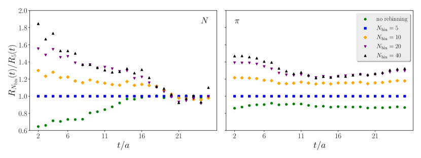
Figure 1: Relative error of the zero-momentum nucleon (left) and pion (right) correlators, denoted $R_{N_{\textup{bin}}}(t)$, for several bin sizes $N_{\textup{bin}}$. All points are normalized by the $N_{\rm bin}=5$ value with errors estimated using the bootstrap procedure with $N_{\textup{B}}=1000$ resamples. All subsequent analysis, which does not employ any correlation functions with $t/a\lesssim 8-10$, ignores autocorrelation and uses $N_{\rm bin}=20$.

3.2 Correlation function construction

The determination of finite-volume nucleon-pion energies requires a diverse set of temporal correlation functions measured on the D200 gauge field ensemble. In addition to diagonal correlation functions between single-pion and single-nucleon interpolating operators, correlation matrices between all operators in each irrep are required. For the $I=3/2$ irreps in Table 1 where the resonant $(2J,\ell)=(3,1)$ partial wave contributes, single-baryon operators are included in addition to nucleon-pion operators resulting in additional valence quark-line topologies. These topologies include those with lines that start and end on the same timeslice.

$N_{\textup{D}}$	$(\rho,n_{\rho})$	$N_{\textup{ev}}$	$N_{\textup{R}}^{\textup{fix}}$	$N_{\textup{R}}^{\textup{rel}}$	Noise dilution	$N_{t_{0}}$
2176	(0.1,36)	448	6	2	(TF,SF,LI16$)_{\textup{fix}}$(TI8,SF,LI16$)_{\textup{rel}}$	4

Table 3: Parameters of the stochastic LapH implementation used to compute temporal correlators in this work. $N_{D}$ is the number of Dirac matrix inversions required per configuration and $(\rho,n_{\rho})$ the stout smearing parameters for the spatial links in the gauge-covariant Laplace operator. $N_{\textup{ev}}$ denotes the dimension of the LapH subspace. $N_{\textup{R}}^{\rm fix}$ and $N_{\rm R}^{\rm rel}$ are the number of stochastic sources for fixed and relative quark lines, respectively. Notation used to specify the dilution scheme for each line type is explained in the text, and the number of source times on each configuration is $N_{t_{0}}$.

Our operator construction is described in Ref. [75] and our method of evaluating the temporal correlators is detailed in Ref. [50]. Well-designed multi-hadron interpolators are comprised of individual constituent hadrons each having definite momenta. Evaluating the temporal correlations of such operators requires all-to-all quark propagators, where all elements of the Dirac matrix inverse are computed. The stochastic-LapH approach [50] enables the efficient treatment of this inverse, provided at least one of the quark fields is LapH smeared [49]. This smearing procedure is effected by a projection onto the space spanned by the $N_{\textup{ev}}$ lowest eigenmodes of the gauge-covariant three-dimensional Laplace operator in terms of link variables which are stout smeared [76] with parameters $(\rho,n_{\rho})$. Although the $N_{\textup{ev}}$ required to maintain a constant smearing radius grows with the spatial volume, the growth of the number of Dirac matrix inversions $N_{\textup{D}}$ can be significantly reduced with the introduction of stochastic estimators in the LapH subspace. Such estimators are specified by the number of dilution projectors in the time (‘T’), spin (‘S’), and Laplacian eigenvector (‘L’) indices, for which ‘F’ denotes full dilution and ‘I$n$’ some number of uniformly interlaced projectors. Different dilution schemes are used for fixed-time quark lines, denoted ‘fix’, which propagate between different timeslices, and relative-time lines (‘rel’) which start and end at the same time. In this work, the relative-time quark lines were only used at the sink time, while the fixed-time lines were used for quark propagation starting and ending at the source time. Both the dilution schemes and the number of stochastic sources used for each type of line are specified in Table 3. Source times $t_{0}=35,64$ were used for correlations going forwards in time, and $t_{0}=64,92$ were used for correlations going backwards in time.

A beneficial property of the stochastic estimators is the factorization of the inverse of the Dirac matrix, which enables correlation construction to proceed in three steps: (1) Dirac matrix inversion, (2) hadron sink/source construction, and (3) correlation function formation. After determining the stochastically-estimated propagators in step (1), the hadron source/sink tensors are computed in step (2). These tensors are subsequently reused to construct many different correlation functions in step (3), which consists of optimized [32] tensor contractions. Averages over the $N_{t_{0}}=4$ different source times (two for forward propagation and two for backward propagation), all possible permutations of the available noise sources in a given Wick contraction, all total momenta of equal magnitude, and all equivalent irrep rows are performed to increase statistics.

3.3 Determination of finite-volume energies

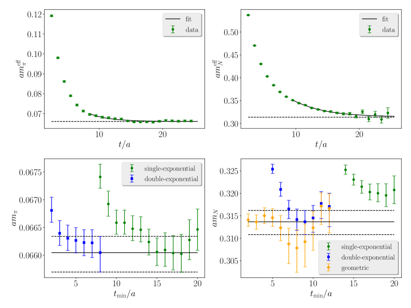
Figure 2: Fits to determine $am_{\pi}$ and $am_{\rm N}$. Bottom row: Variation of the fit range $[t_{\rm min},t_{\rm max}]$ with $t_{\rm max}=25a$ for correlated-$\chi^{2}$ fits. Both single- and double-exponential fits are shown and the horizontal band indicates the two-exponential fit range chosen so that statistical errors are dominant. Top row: the chosen two-exponential fits overlayed on standard effective masses for $am_{\pi}$ (left) and $am_{\rm N}$ (right).

Once the correlation functions computed as described in Sec. 3.2 are available, the determination of finite-volume energies can commence. From the (binned) correlator and reweighting factor measurements, the reweighted correlation functions are computed as secondary observables according to Eq. (6). Their statistical errors and covariances are used in fits to determine energies and estimated by the bootstrap procedure with $N_{\rm B}=800$ samples.

In order to ensure that $t_{\rm bnd}$ is sufficiently large, a maximum time separation $t_{\rm max}=25a$ is enforced globally in the analysis. Energies are determined from correlated-$\chi^{2}$ fits to both single- and two-exponential fit forms, which are additionally compared to a “geometric series” form

$$C(t)=\frac{A{\rm e}^{-Et}}{1-B{\rm e}^{-Mt}},$$ (7)

which consists of four free parameters. We also explored a “multi-exponential” variant of the geometric series, with the replacement $Be^{-Mt}\rightarrow\sum_{n}B_{n}e^{-M_{n}t}$.

The application of our approach to determining the nucleon and pion masses is shown in Fig. 2. As usual, a fit range is desired so that statistical errors on the energies are larger than systematic ones. This optimal range is selected according to several criteria. First, a good fit quality $q\gtrsim 0.2-0.3$ is enforced to ensure that the fit describes the data within the usual 68% confidence interval quoted for statistical errors. Second, the absence of any statistically significant change in the energy upon variation of $t_{\rm min}$ around the chosen fit range further suggests that the asymptotic large-time behavior is applicable. Finally, consistency across different fit forms supports the hypothesis that the energy determination is statistics limited. For the pion, consistency between single- and two-exponential fits, as well as the mild variation with $t_{\rm min}$, suggests that statistical errors are dominant. As is evident in $am^{\rm eff}_{\rm N}$, single-exponential fits for $am_{\rm N}$ are unsuitable, but consistency between the double-exponential and geometric fit forms is reassuring.

For the nucleon-pion channels, excited state energies are determined in addition to ground states. This requires a large basis of interpolating operators in each irrep and two-point correlations between them. The resulting $N_{\rm op}\times N_{\rm op}$ hermitian matrix, denoted $C_{ij}(t)$, is rotated [77] using eigenvectors $v_{n}(t_{0},t_{\rm d})$ of the generalized eigenvalue problem (GEVP)

$$C(t_{\rm d})v_{n}(t_{0},t_{\rm d})=\lambda_{n}(t_{0},t_{\rm d})C(t_{0})v_{n}(t_{0},t_{\rm d}).$$ (8)

In our single-pivot approach, the correlation matrix is rotated by these vectors for all $t$, and the diagonal elements of the rotated matrix, denoted $D_{n}(t)$, are correlators with optimal overlap onto the lowest $N_{\rm op}$ states. Although diagonalizing separately on each time-slice ensures that the optimized correlators are increasingly dominated by the desired state for asymptotically large times [78, 79], in practice, the single-pivot method produces nearly identical results if $(t_{0},t_{\rm d})$ are chosen appropriately. Systematic errors related to this are controlled by ensuring that extracted energies are insensitive to $(t_{0},t_{\rm d})$ and $N_{\rm op}$ and by ensuring that the rotated correlation matrix remains diagonal within statistical errors for all time separations $t>t_{\rm d}$. The advantages of diagonalizing on a single set of times include a better signal-to-noise ratio for large times and no need for eigenvector pinning in which eigenvectors are re-ordered for diagonalizations at different times and bootstrap samples.

After forming the optimized correlators, the following ratio is taken

$$R_{n}(t)=\frac{D_{n}(t)}{C_{\pi}(\bm{d}_{\pi}^{2},t)\,C_{\rm N}(\bm{d}_{\rm N}^{2},t)},$$ (9)

with $\bm{d}_{\pi}^{2}$ and $\bm{d}_{\rm N}^{2}$ chosen so that

$$E_{n}^{\rm non.\,int.}=\sqrt{m_{\pi}^{2}+\left(\frac{2\pi\bm{d}_{\pi}}{L}\right)^{2}}+\sqrt{m_{\rm N}^{2}+\left(\frac{2\pi\bm{d}_{\rm N}}{L}\right)^{2}}$$ (10)

corresponds to the closest non-interacting energy. The ratio $R_{n}(t)$ is then fit to the single-exponential ansatz $R_{n}(t)=A_{n}\textup{e}^{-\Delta E_{n}t}$ to determine the energy shift $a\Delta E_{n}$, from which the lab-frame energy is reconstructed $aE_{n}^{\textup{lab}}=a\Delta E_{n}+aE_{n}^{\textup{non.int.}}$. Although the ratio fits enable somewhat smaller $t_{\textup{min}}$ when $\Delta E_{n}$ is small, they offer little advantage for states which are significantly shifted from non-interacting levels. Nonetheless, ratio fits are employed for all levels in the nucleon-pion irreps, and are typically consistent with single- and double-exponential fits directly to $D_{n}(t)$.

A sample illustration of the procedure for nucleon-pion energies is shown in Fig. 3 for the second level in the $I=1/2$ $G(3)$ irrep. Due to partial wave mixing, the single-nucleon state is also present in this irrep. The GEVP is therefore required to properly isolate the desired higher-lying nucleon-pion energies. Analogous plots for all levels are given in A and B for the GEVP- and $t_{\rm min}$-stability plots, respectively.

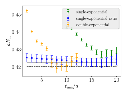
Figure 3: Example determination of the spectrum in the $I=1/2$ $G(3)$ irrep. Left: $t_{\rm min}$-plot for the second level including single- and two-exponential fits to $D_{n}(t)$ as well as single-exponential fits to the ratio $R_{n}(t)$ in Eq. (9). All fits employ the GEVP of Eq. (8) with $N_{\rm op}=4$ and $(t_{0},t_{\rm d})=(8a,16a)$. The horizontal band represents the chosen $t_{\rm min}$ from the ratio fit. Right: stability under variation of the GEVP parameters for the entire spectrum in this irrep. For each level $t_{\rm min}$ is fixed while $(N_{\rm op},t_{0},t_{\rm d})$ are varied as shown in the legend. The elastic and inelastic thresholds are represented by dotted lines.

The spectra resulting from this analysis are shown in Figs. 4(a) and 4(b) for the $I=1/2$ and $I=3/2$ channels, respectively.

4 Scattering parameter results and discussion

This section details the determination of the scattering parameters from the finite-volume energies. The parameterizations of the $K$ matrix elements are presented, and best-fit values for the parameters are summarized. Lastly, a comparison with chiral perturbation theory is made.

4.1 Scattering parameter determinations

The energies shown in Figs. 4(a) and 4(b) are next used to determine scattering amplitudes via the relations in Sec. 2. Although these relations are only applicable to energies below the nucleon-pion-pion threshold, the slow growth of three-body phase space near threshold suppresses corrections to Eq. (3) and the coupling of nucleon-pion-pion states to our operator basis is naively suppressed by the spatial volume, so energies somewhat above the inelastic threshold are expected to be appropriate for inclusion in our global fits. Nevertheless, we restrict our attention to center-of-mass energies below or within one standard deviation of the threshold $E_{\rm cm}=2m_{\pi}+m_{\rm N}$.

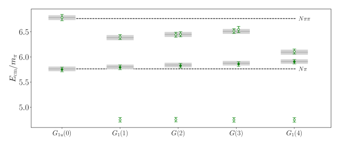
(a) The $I=1/2$ spectrum.

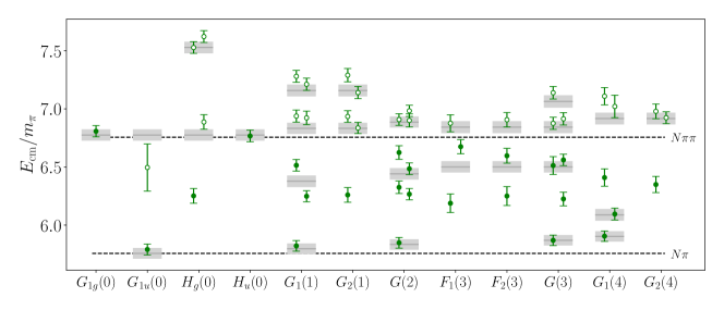
(b) The $I=3/2$ spectrum.

Figure 4: The low-lying $I=1/2$ and $I=3/2$ nucleon-pion spectra in the center-of-momentum frame on the D200 ensemble described in Table 2. Each column corresponds to a particular irrep $\Lambda$ of the little group of total momentum $\bm{P}^{2}=(2\pi/L)^{2}\bm{d}^{2}$, denoted $\Lambda(\textbf{{d}}^{2})$. Dashed lines indicate the boundaries of the elastic region. Solid lines and shaded regions indicate non-interacting $N\pi$ levels and their associated statistical errors. Levels employed in subsequent fits to constrain the scattering amplitudes are shown with solid symbols. For $I=3/2$, all well-constrained levels with overlap below the $N\pi\pi$ threshold are included. For the $I=1/2$ channel, we are only interested in the scattering length, so only the ground state in each irrep is used to determine the $I=1/2$ amplitude near the $N\pi$ threshold.

The goal of this analysis is a parametrization of the $J^{P}=1/2^{-}$ partial wave for both isospins, and the $3/2^{+}$ wave with $I=3/2$. As discussed in Sec. 2, energies from irreps with zero total momentum directly provide points for these partial waves up to corrections from $\ell\geq 3$ contributions. However, mixing among the desired waves, as well as with others, generally occurs for energies in irreps with non-zero total momentum. The zero-momentum points are therefore a useful guide when plotted together with the partial wave fits.

Each partial wave is parametrized using the effective range expansion. For the $I=3/2$, $J^{P}=3/2^{+}$ wave, the next-to-leading order is included

$$\frac{q_{\rm cm}^{3}}{m_{\pi}^{3}}\cot\delta_{3/2^{+}}=\frac{6\pi\sqrt{s}}{m^{3}_{\pi}g_{\Delta,{\rm BW}}^{2}}(m_{\Delta}^{2}-s),$$ (11)

where $\sqrt{s}=E_{\rm cm}=\sqrt{m_{\pi}^{2}+q_{\rm cm}^{2}}+\sqrt{m_{N}^{2}+q_{\rm cm}^{2}}$, and the effective range fit parameters are reorganized to form the conventional Breit-Wigner properties of the $\Delta(1232)$ resonance, denoted $g_{\Delta,{\rm BW}}^{2}$ and $m_{\Delta}$. For the other waves, the leading term in the effective range expansion is sufficient

$$\frac{q_{\rm cm}^{2\ell+1}}{m_{\pi}^{2\ell+1}}\cot\delta^{I}_{J^{P}}=\frac{\sqrt{s}}{m_{\pi}A^{I}_{J^{P}}},$$ (12)

where the overall $\sqrt{s}$ factors are adopted from standard continuum analysis [80], and the single fit parameter $A_{J^{P}}^{I}$ is trivially related to the scattering length

$$m_{\pi}^{2\ell+1}a_{J^{P}}^{I}=\frac{m_{\pi}}{m_{\pi}+m_{N}}A^{I}_{J^{P}}.$$ (13)

Two different fit strategies are employed to determine the parameters from the finite-volume energies. The first, called the “spectrum method” [81], obtains best-fit values of the model parameters $\{p_{n}\}$ by minimizing

$$\chi^{2}\left(\left\{p_{n}\right\}\right)=\sum_{ij}\left(\frac{q_{{\rm cm},i}^{2}}{m_{\pi}^{2}}-\frac{q_{{\rm cm},i}^{2,\textrm{QC}}}{m_{\pi}^{2}}\left(\left\{p_{n}\right\}\right)\right)C_{ij}^{-1}\left(\frac{q_{{\rm cm},j}^{2}}{m_{\pi}^{2}}-\frac{q_{{\rm cm},j}^{2,\textrm{QC}}}{m_{\pi}^{2}}\left(\left\{p_{n}\right\}\right)\right),$$ (14)

where the $q_{{\rm cm},i}^{2}$ are the center-of-mass momenta squared computed from lattice QCD, with covariance matrix $C$, and $q_{{\rm cm},i}^{2,\textrm{QC}}\left(\left\{p_{n}\right\}\right)$ are the center-of-mass momenta squared evaluated from the model fit form for a given choice of parameters $\left\{p_{n}\right\}$. The fact that the model depends on $m_{\rm N}/m_{\pi}$, and is therefore not independent of the data to be fit, complicates the evaluation of the covariance matrix $C$. As discussed in Ref. [57], a simple way to avoid this complication so that $C$ is just the covariance matrix of the data is to introduce model parameters for $m_{\pi}L$ and the ratio $m_{\rm N}/m_{\pi}$, and include appropriate additional terms in the $\chi^{2}$ of Eq. (14). Given the relatively small errors on $m_{\rm N}/m_{\pi}$ and $m_{\pi}L$, these additional terms have little effect on the fit parameters and the resultant $\chi^{2}$, and are subsequently ignored. Note that the evaluation of the $(q_{{\rm cm},i}^{2,{\rm QC}}/m_{\pi}^{2})(\{p_{n}\})$ for a particular choice of the parameters requires the determination of roots of Eq. (3), a procedure which can be delicate for closely-spaced energies.

The second method, called the “determinant residual” method [57], employs the determinants of Eq. (3) themselves as the residuals to be minimized. These determinants depend on the fit parameters through the $K$-matrix, which are adjusted to minimize the residuals and best satisfy Eq. (3). This approach avoids the subtleties associated with root-finding, but has other difficulties. For the spectrum method, the covariance between the residuals is, to a good approximation, simply the covariance between the $q_{{\rm cm},i}^{2}/m_{\pi}^{2}$, which can be estimated once and does not depend on the fit parameters. Conversely, for the determinant residual method, the covariance must be re-estimated whenever the parameters are changed. Since the statistical errors on the determinant are typically larger than those on $q_{{\rm cm},i}^{2}/m_{\pi}^{2}$, this approach is less sensitive to higher partial waves, and results in a smaller $\chi^{2}$ compared to the spectrum method.

Fit	$N_{\rm pw}$	$A_{1/2^{-}}$	$g_{\Delta,{\rm BW}}$	$M_{\Delta}/M_{\pi}$	$A_{1/2^{+}}$	$A_{3/2^{-}}$	$A_{5/2^{-}}$	$\chi^{2}$	dofs
SP	2	$-1.56(4)$	13.8(6)	6.281(16)	—	—	—	44.38	$23-3$
DR	2	$-1.57(5)$	14.4(5)	6.257(36)	—	—	—	14.91	$23-3$
SP	5	$-1.53(4)$	14.7(7)	6.290(18)	$-0.19(6)$	$-0.46(12)$	0.37(10)	30.17	$25-6$

Table 4: Results for the fits in the $I=3/2$ channel. $N_{\rm pw}$ is the number of partial waves included in the fit. Two different fit forms are included, the one denoted $N_{\rm pw}=2$ includes only the desired partial waves, namely $J^{P}=1/2^{-}$ and $3/2^{+}$, while the one with $N_{\rm pw}=5$ includes all $s$-, $p$-, and $d$-waves, employing the two additional energy levels in the $G_{\rm 1g}(0)$ and $H_{\rm u}(0)$ irreps. For the $N_{\rm pw}=2$ fit, results from the determinant-residual method, denoted ‘DR’, are shown in addition to the spectrum method, denoted ‘SP’.

Fit	$N_{\rm pw}$	$A_{1/2^{-}}$	$\chi^{2}$	dofs
SP	1	0.82(12)	1.68	$5-1$
DR	1	0.92(22)	1.72	$5-1$
SP	1	0.82(13)	0.79	$4-1$

Table 5: Results for fits to the $I=1/2$ spectrum in Fig. 4(a). $N_{\rm pw}$ is the number of partial waves included in the fit. Due to the small number of levels, all fits include only the desired $J^{P}=1/2^{-}$ partial wave. Nonetheless, the effect of the omitted $p$-waves is estimated by removing the $G_{1}(4)$ level, which evidently has little influence on the result. ‘SP’ refers to the spectrum method, and ‘DR’ refers to the determinant-residual method.

For the $I=3/2$ fits, the $J^{P}=1/2^{+}$, $3/2^{-}$, and $5/2^{-}$ partial waves are added to the spectrum method fits along with the ground states in the $G_{\rm 1g}(0)$ and $H_{\rm u}(0)$ irreps. The $I=3/2$ spectrum in the $G_{\rm 2g}(0)$ irrep was not computed, and irreps in the $I=1/2$ channel which do not contain the $s$-wave were also omitted. This choice was made for computational simplicity, although these irreps may be beneficial to further constrain higher partial waves in future work. The determinant residual method was found to be less able to constrain higher partial waves and was only used in fits that included just the $J^{P}=1/2^{-}$, $3/2^{+}$ waves. Nonetheless, the consistency between these different fitting methods, as well as those including higher partial waves, suggest that uncertainties on amplitude parameters are statistics dominated.

For the $I=1/2$ channel, $\ell_{\rm max}=0$ is employed. Although the small number of levels precludes a sophisticated estimate of the effect of higher partial waves, the influence of the omitted $p$-waves can be explored by examining the influence of the highest-lying level on the fit. Table 5 indicates that the effective range is insensitive to the omission of the lowest-lying nucleon-pion level in the $G_{1}(4)$ irrep. These $I=1/2$ fits are also insensitive to an additional term in the effective range expansion, and exhibit no statistically significant difference between the spectrum and determinant-residual methods.

Results from fits using both the spectrum and determinant-residual methods including various partial waves are given in Tables 4 and 5 for $I=3/2$ and $I=1/2$, respectively. In addition to the desired partial waves, fits using the spectrum method are mildly sensitive to the $J^{P}=1/2^{+}$, $3/2^{-}$, and $5/2^{-}$ waves with $I=3/2$. Although not included in the table, the determination of the effective range for both isospins is robust to the addition of the next term in the effective range expansion. Results for the partial waves from the fit including only the desired partial waves are shown with the points from the total-zero momentum irreps in Figs. 5 and 6 for the $I=3/2$ and $I=1/2$ partial waves, respectively. The phase shift $\delta_{3/2^{+}}$ has the characteristic profile of the $\Delta(1232)$ resonance and is shown in Fig. 7. Since the scattering length is the only desired parameter from the $I=1/2$ spectrum, only the lowest nucleon-pion levels from each irrep are included in the fit, as denoted by the solid symbols in Fig. 4(a). Full exploration of the elastic $I=1/2$ spectrum likely requires additional operators beyond the scope of this work, due to the strongly-interacting $J^{P}=1/2^{+}$ wave containing the $N(1440)$ Roper resonance.

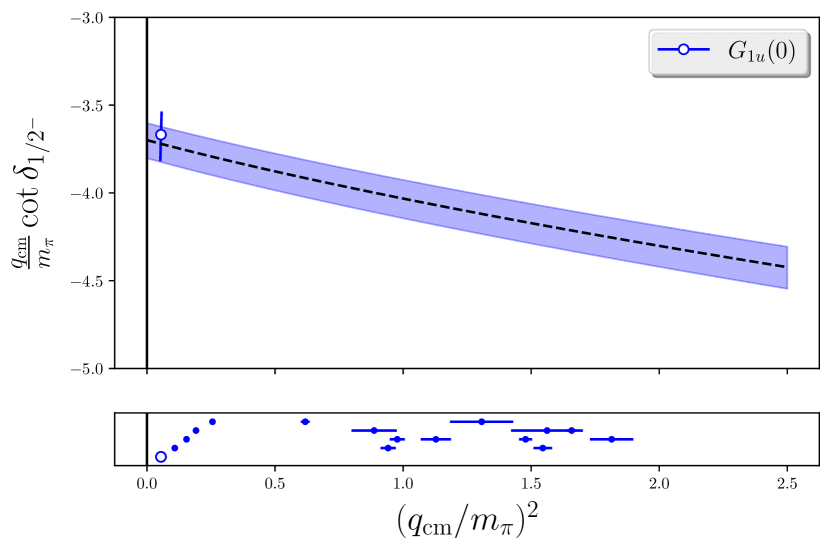
(a) $J^{P}=1/2^{-}$

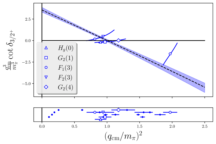
(b) $J^{P}=3/2^{+}$

Figure 5: The results from fits to the $I=3/2$ spectrum in Fig. 4(b) using the spectrum method including the $J^{P}=1/2^{-},3/2^{+}$ partial waves only, omitting the $H_{\rm u}(0)$ and $G_{1\rm g}(0)$ irreps. The lower panel of each partial wave shows the squares of the center-of-mass momenta of the finite-volume levels which contribute to fitting that partial wave. Most levels, shown with solid symbols, contribute to both partial waves, so solving for the partial wave phase shift shown in the upper panel cannot be done. When a particular level couples only to the partial wave shown, a phase shift point can be obtained from the energy level and is shown in the upper panel. Hollow symbols indicate such levels. For clarity, the levels in the lower panel are vertically spaced according to the (integer-valued) total momentum $\bm{d}^{2}$.

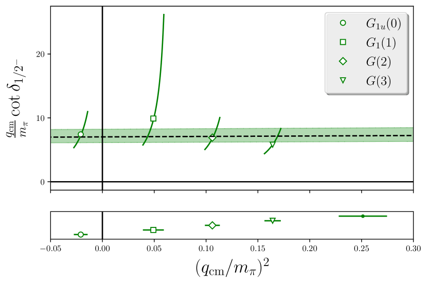
Figure 6: The result of fits to the $I=1/2$ spectrum in Fig. 4(a) to determine the scattering length of the $J^{P}=1/2^{-}$ wave. As in Fig. 5, the lower panel shows the input spectra. For $\ell_{\rm max}=0$, even levels with total non-zero momentum result in phase shift point in the upper panel. The level with largest $q_{\rm cm}^{2}$ is not shown in the upper panel due to its large error.

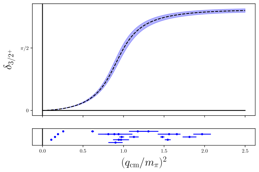
Figure 7: Scattering phase shift of the $I=3/2$, $J^{P}=3/2^{+}$ partial wave containing the $\Delta(1232)$ resonance. The curve is obtained from a fit of the finite-volume energies shown in the lower panel using Eq. (3) and a Breit-Wigner form. The energies are computed on the single $N_{\rm f}=2+1$ lattice QCD gauge field ensemble with $a=0.065$ fm and $m_{\pi}=200$ MeV described in Table 2. Levels used in the fit are shown in the lower panel, similar to Figs. 5 and 6, but no data points are shown in the upper panel to more clearly show the final fit form.

The spectrum method enables an additional visualization of the quality of fits to the finite-volume spectra. The residual is constructed using model values of $q_{\rm cm}^{2,{\rm QC}}/m_{\pi}^{2}$ which depend on the parameters and can be compared with the input data from the spectrum. Such comparisons are shown in Fig. 8 for both the $I=1/2$ and $I=3/2$ spectra. Although not shown explicitly on the plot, the ground states in $G_{1}(1)$, $G(2)$, $G(3)$, and $G_{1}(4)$ with $I=3/2$ are sensitive to the $J^{P}=3/2^{+}$ partial wave. The $\ell_{\rm max}=0$ approximation significantly increases the $\chi^{2}$ for these levels. Conversely, these levels therefore place significant constraints on the near-threshold behavior of the $3/2^{+}$ wave, in contrast to the higher-lying levels in the $H_{g}(0)$, $G_{2}(1)$, $F_{1}(3)$, $F_{2}(3)$, and $G_{2}(4)$ irreps. The ground states in the $G_{1\rm g}(0)$ and $H_{\rm u}(0)$ irreps are not shown on the plot, and only included in the $N_{\rm pw}=5$ fit in Table 4.

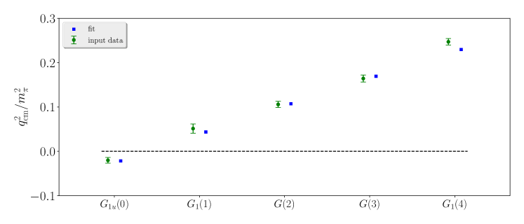
(a) The $I=1/2$ spectrum compared with model values.

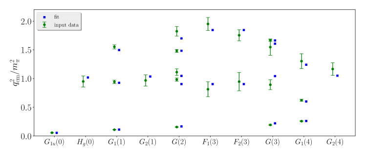
(b) The $I=3/2$ spectrum compared with model values.

Figure 8: The center-of-mass momentum $q_{\rm cm}^{2}/m_{\pi}^{2}$ for the $I=1/2$ and $I=3/2$ spectra together with model values from amplitude fits employing the spectrum method with $N_{\rm pw}=2$ partial waves for $I=3/2$. For $I=1/2$, only the $s$-wave is included and the fit to all five points is shown.

The final results for the scattering lengths in this work are taken from the determinant residual method fit in Table 4 with $N_{\rm pw}=2$ for $I=3/2$ and the spectrum method fit for $I=1/2$ including all five levels

$$m_{\pi}a_{0}^{3/2}=-0.2735(81)\,,\qquad m_{\pi}a_{0}^{1/2}=0.142(22),$$ (15)

which are already given in Eq. (1). In Fig. 9, the results from this work for the Breit-Wigner parameters of the $\Delta(1232)$ resonance in the $I=3/2$, $J^{P}=3/2^{+}$ partial wave are compared to the published numbers in Refs. [40] and [82]

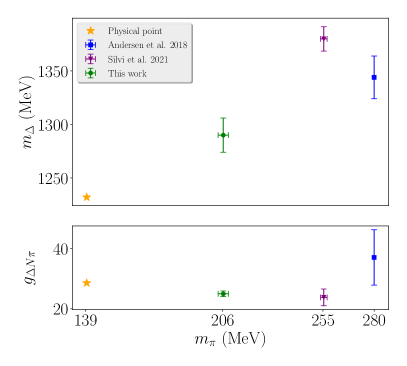
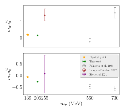
Figure 9: Comparison of results from this work to previous lattice calculations. Top left: the Breit-Wigner mass $m_{\Delta}$. Bottom left: the coupling $g_{\Delta N\pi}$ from leading-order effective field theory. Top right: the $N\pi$ isodoublet scattering length $m_{\pi}a_{0}^{1/2}$ in terms of the pion mass. Bottom right: the $N\pi$ isoquartet scattering length $m_{\pi}a_{0}^{3/2}$. Prior results are indicated by ‘Anderson et al. 2018’ [40], ‘Silvi et al. 2021’ [82], ‘Fukugita et al. 1995’ [42], and ‘Lang and Verduci 2012’ [39]. Physical point values are obtained using Refs. [93, 94, 92].

where, as is customary, the definition of the $g_{\Delta N\pi}$ coupling from leading-order effective field theory is used, as defined in Eq. (39) of Ref. [82]. When considering Fig. 9, keep in mind that the quark mass trajectory used here and in Ref. [40], which fixes the sum of the quark masses, differs from that used in Ref. [82], which fixes the strange quark mass to its physical value. A comparison of the scattering lengths determined here to past lattice QCD results is also shown in Fig. 9.

4.2 Comparison with phenomenology and chiral perturbation theory

Although the results here are only at a single pion mass, it is interesting to compare our scattering lengths to those extracted phenomenologically [83, 84] from pionic atoms [85, 86, 87], as well as to those obtained from chiral perturbation theory. The proximity of $m_{\pi}=200$ MeV to its physical value naively suggests that $SU(2)$ baryon $\chi$PT may be applicable. While $\chi$PT may be poorly converging for $g_{A}$ and $m_{N}$, the convergence pattern is an observable dependent issue which has not been explored for $N\pi$ scattering.

Pionic hydrogen ($\pi H$) is sensitive to one combination of the isoscalar ($a^{+}$) and isovector ($a^{-}$) scattering lengths and pionic deuterium ($\pi D$) is sensitive to a different combination, allowing for a percent level determination [83, 84]. Phenomenological values extracted from a full $\pi N$ partial wave analysis have been reported in Ref. [88]. Ref. [27] determined the values of these scattering lengths in the isospin limit. While it is customary for the lattice community to use $m_{\pi}=135$ MeV as the pion mass in the isospin limit, it is common in the phenomenological estimates to use the charged pion mass to determine the QCD quantities in the absence of QED corrections. In order to be consistent with the phenomenological estimates, we similarly use the charged pion mass when quoting results at the physical pion mass.

These scattering lengths are known to fourth order in the baryon chiral expansion [89, 90, 91] and expressed in Appendix F of Ref. [88] and Ref. [92] in a form convenient for extrapolating LQCD results. In terms of the $s$-wave $a_{0}^{\pm}$ scattering lengths, the isospin 1/2 and 3/2 $\pi N$ scattering lengths are given by

$$a_{0}^{3/2}=a_{0}^{+}-a_{0}^{-}\,, a_{0}^{1/2}=a_{0}^{+}+2a_{0}^{-}\,.$$ (16)

At leading order (LO), the scattering lengths are free of LECs and given by

$$m_{\pi}a_{0}^{3/2}[{\rm LO}]=-\epsilon_{\pi}^{2}\frac{2\pi}{1+\mu}\,, m_{\pi}a_{0}^{1/2}[{\rm LO}]=\epsilon_{\pi}^{2}\frac{4\pi}{1+\mu}\,,$$ (17)

where

$$\epsilon_{\pi}=\frac{m_{\pi}}{4\pi F_{\pi}}, \mu=\frac{m_{\pi}}{m_{N}}.$$ (18)

The values of these input parameters on D200 and at the physical (charged) pion mass are

$$\epsilon_{\pi}^{\rm D200}=0.1759(12), \mu^{\rm D200}=0.2102(19),$$

$$\epsilon_{\pi}^{\rm phys}=0.12064(74), \mu^{\rm phys}=0.14875(05)\,.$$ (19)

	$m_{\pi}$ (MeV)	$\ \ m_{\pi}a_{0}^{1/2}$	$\quad\ m_{\pi}a_{0}^{3/2}$
This work	200	$0.142(22)$	$-0.2735(81)$
LO $\chi$PT	200	$0.321(04)(57)$	$-0.161(02)(28)$
LO $\chi$PT	140	$0.159(02)(19)$	$-0.080(01)(10)$
Pheno. (isospin limit)[27]	140	$0.1788(38)$	$-0.0775(35)$

Table 6: A comparison of our $N\pi$ scattering length results at $m_{\pi}=200$ MeV with phenomenological values in the isospin limit and predictions from leading order chiral perturbation theory. For the $\chi$PT predictions, the first error is from uncertainties on the input parameters, $\epsilon_{\pi}$ and $\mu$, and the second error is a $\chi$PT truncation uncertainty given by $\epsilon_{\pi}m_{\pi}a_{0}^{I}[\rm LO]$.

A comparison of our results with the LO $\chi$PT predictions and phenomenological values in the isospin limit from Ref. [27] is presented in Table 6. Not only do our results disagree with LO $\chi$PT, but we also find the magnitude of $m_{\pi}a_{0}^{3/2}$ exceeds that of $m_{\pi}a_{0}^{1/2}$, in conflict with both LO $\chi$PT and phenomenology. Note that the LO $\chi$PT predictions at the physical point are in reasonable agreement with the phenomenological values, lying within one sigma of the estimated $\chi$PT truncation uncertainty. With only one pion mass available in this work, the reasons for the discrepancy of our results with LO $\chi$PT cannot be ascertained. Interestingly, our scattering length results can be described at next-to-leading order (NLO) using a single LEC. At NLO, one finds

$$m_{\pi}a_{0}^{3/2}[{\rm NLO}] =-\epsilon_{\pi}^{2}\frac{2\pi}{1+\mu}\left\{1+\frac{\epsilon_{\pi}}{2}\frac{\Lambda_{\chi}}{m_{N}}(g_{A}^{2}+8C)\right\}\,,$$

$$m_{\pi}a_{0}^{1/2}[{\rm NLO}] =\phantom{-}\epsilon_{\pi}^{2}\frac{2\pi}{1+\mu}\left\{1-\frac{\epsilon_{\pi}}{4}\frac{\Lambda_{\chi}}{m_{N}}(g_{A}^{2}+8C)\right\}\,,$$ (20)

where $\Lambda_{\chi}=4\pi F_{\pi}$ and we have defined the dimensionless LEC

$$C=m_{N}(2c_{1}-c_{2}-c_{3})\,,$$ (21)

in terms of the $c_{i}$ LECs in the baryon chiral Lagrangian [95]. The scattering lengths in this work can be described by these NLO formulae if $C$ is in the range 0.6-0.7. The NLO phenomenological determination finds a value of $C\approx 0.3$, which is not significantly different from that needed to describe our results. However, the phenomenological extraction of the LECs in Ref. [88] is clouded by issues related to the $\Delta$ degrees of freedom [20] and is not stable until at least next-to-next-to-next-to-leading order (N³LO) [88]. When results at additional pion masses, particularly lighter ones, become available, a more thorough understanding of the pion mass dependence of the scattering lengths can be achieved and a more quantitative comparison with the results from the phenomenological analysis and $\chi$PT can be performed.

5 Conclusion

This work presents a computation of the lowest partial waves for the elastic nucleon-pion scattering amplitude on a single ensemble of gauge configurations with $m_{\pi}=200~{}{\rm MeV}$. The $s$-wave scattering lengths are determined for both isospins $I=1/2$ and $I=3/2$ and compared to determinations from LO $\chi$PT and a Roy-Steiner analysis[88]. To our knowledge, this is the first (unquenched) lattice QCD determination of both nucleon-pion scattering lengths for $m_{\pi}<250$ MeV. The Breit-Wigner resonance parameters of the $\Delta(1232)$ in the $J^{P}=3/2^{+}$ partial wave with $I=3/2$ are determined as well.

A comparison of two different methods, the spectrum method and the determinant residual method, of extracting $K$-matrix information from finite-volume spectra is also performed. Although the determinant residual method avoids awkward root-finding, it was found to be less sensitive to higher partial wave contributions. Nonetheless, the consistency between these two different fitting procedures is reassuring.

These results suggest that the methods used here will prove useful for future work at the physical values of the quark masses and for other lattice spacings. Larger volumes needed at smaller quark masses will require an increase of $N_{\rm ev}$, the dimension of the LapH subspace discussed in Sec. 3.2, but not the number of Dirac matrix inversions in the stochastic-LapH algorithm for all-to-all quark propagators. Nevertheless, the increasingly severe signal-to-noise problem will likely require more configurations and source times to achieve a similar statistical precision.

This work is part of a larger effort to compute baryon scattering amplitudes on lattice QCD gauge field ensembles at quark masses in the chiral regime $m_{\pi}\lesssim 300~{}{\rm MeV}$ where effective theories may be applicable. As discussed in Sec. 3.2, the stochastic LapH approach to quark propagation enables considerable re-use of the hadron tensors in multiple multi-hadron correlation functions on the D200 ensemble employed here. Analyses are currently underway to compute the analogous amplitudes for the $N\Lambda-N\Sigma$ and $NN$ systems. Hopefully this exploratory computation has sufficient statistical precision to impact chiral effective theories for these baryon-baryon channels as well.

Appendix A Systematic errors from correlation matrix rotation

As discussed in Sec. 3.3, the optimized diagonal correlation functions $D_{n}(t)$ are obtained in this work from the GEVP using a single-pivot approach which uses one choice of $(t_{0},t_{\rm d})$. The systematic error associated with this approach is estimated for each energy level by fixing the fit range $[t_{\rm min},t_{\rm max}]$ and varying the GEVP metric and diagonalization times $(t_{0},t_{\rm d})$ defined in Eq. (8), as well as the dimension of the input correlation matrix $N_{\rm op}$. Taking both GEVP stability and statistical precision into account, the parameters $(t_{0},t_{\rm d})=(8a,16a)$ are found to work well for all energies presented here. As shown in Fig. 10, the spectrum is rather insensitive to variations in $(t_{0},t_{\rm d})$ and $N_{\rm op}$.

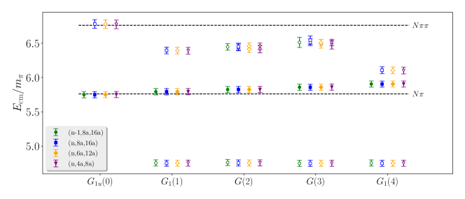
(a) the $I=1/2$ spectrum.

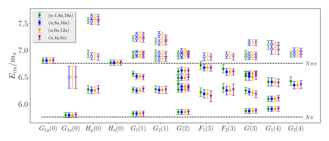
(b) the $I=3/2$ spectrum.

Figure 10: Stability of the finite-volume spectra under variation of the GEVP as discussed in Sec. 3.3. Multiple values of $(N_{\rm op},t_{0},t_{\rm d})$ for each level are shown with a horizontal displacement for clarity. Each irrep is shown in a column in the same manner as Fig. 4 with $n$ denoting the maximum $N_{\textup{op}}$.

Appendix B Systematic errors from varying fit forms and time ranges

As discussed in Sec. 3.3, multiple fit ranges and fit forms are compared for every energy level to ensure systematic errors associated with excited state contamination are smaller than the statistical errors. Ultimately, single-exponential fits to the correlator ratios in Eq. (9) are chosen due to their mild sensitivity to $t_{\textup{min}}$ and good statistical precision. The fit range is chosen to be consistent with the double-exponential $t_{\textup{min}}$ plateau, defined as the range of $t_{\rm min}$ for which the fitted energy exhibits no statistically significant variation. Most levels are additionally consistent with the single-exponential fit plateau, although as shown in Fig. 2 for $m_{\rm N}$, these fits may fail to describe correlators with significant excited-state contamination. Plots analogous to the $t_{\rm min}$-plot in Fig. 3 are shown for each of the $I=1/2$ levels in Fig. 11 and the $I=3/2$ levels in Figs. 13-21.

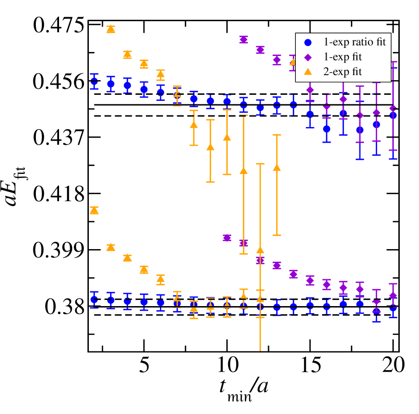
(a) $G_{1u}(0)$

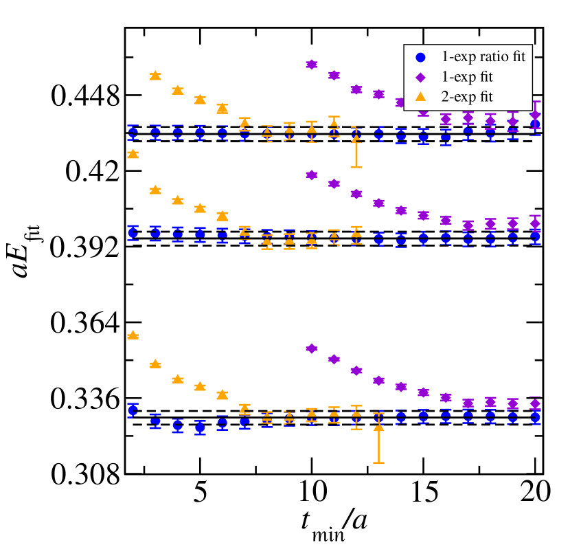
(b) $G_{1}(1)$

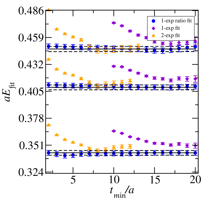
(c) $G(2)$

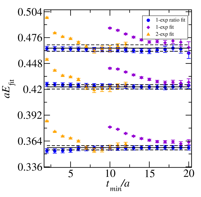
(d) $G(3)$

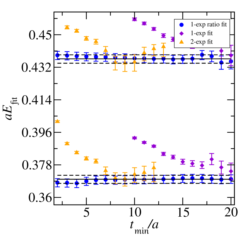
(e) $G_{1}(4)$

Figure 11: Stability of the $I=1/2$ spectrum illustrated by varying the fit range and fit form. The chosen fit for each level is indicated by the solid black line and the corresponding errors are indicated by dotted lines. Each subplot contains the spectrum for a single irrep labeled in the same manner as Fig. 4. The chosen values are taken from ratio fits and compared to both single- and double-exponential fits over a range of $t_{\textup{min}}$ with $t_{\rm max}=25a$.

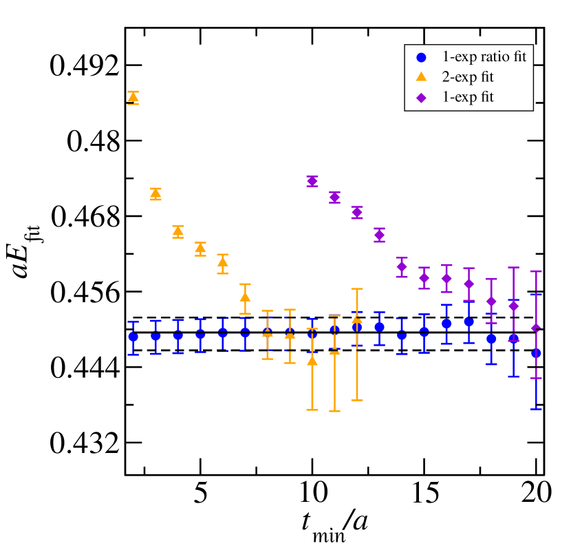
(a) $G_{1g}(0)$ level 0

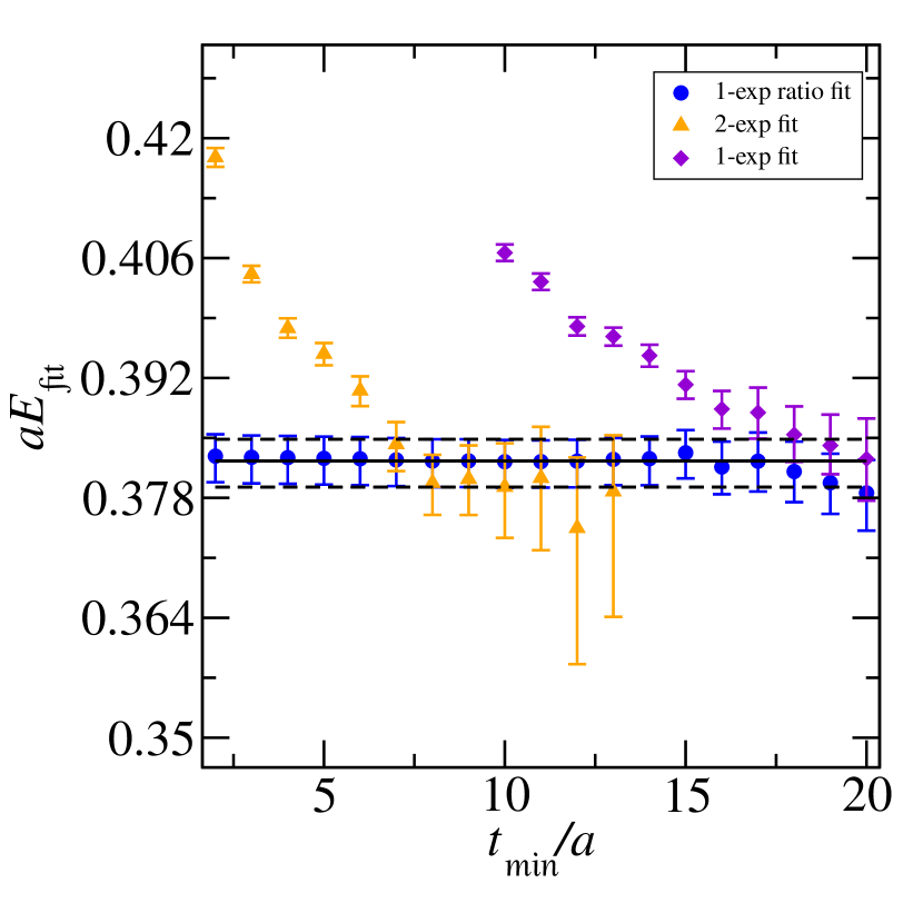
(b) $G_{1u}(0)$ level 0

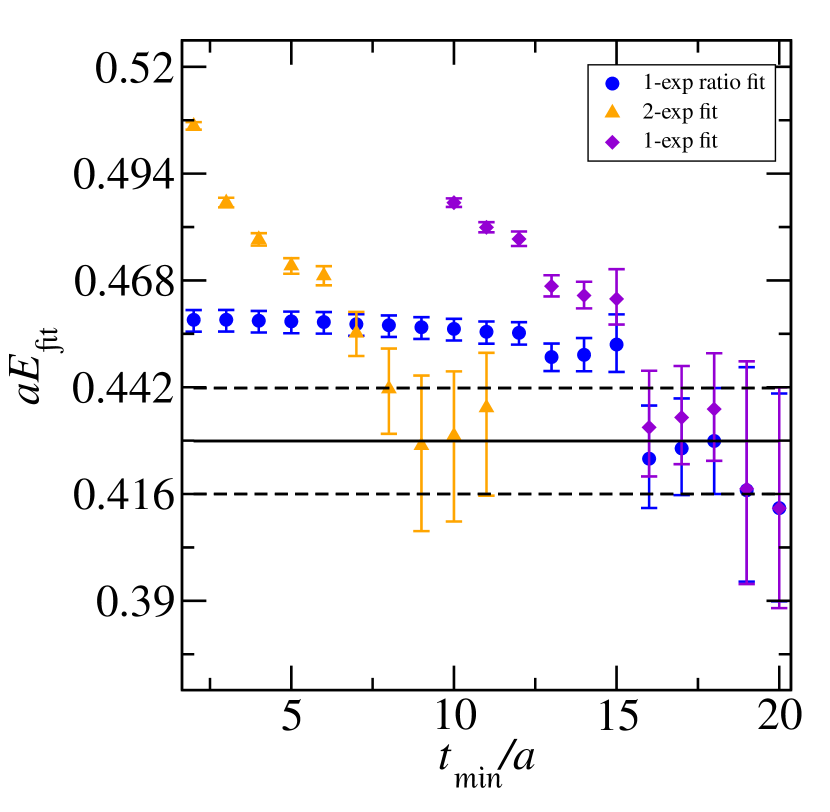
(c) $G_{1g}(0)$ level 1

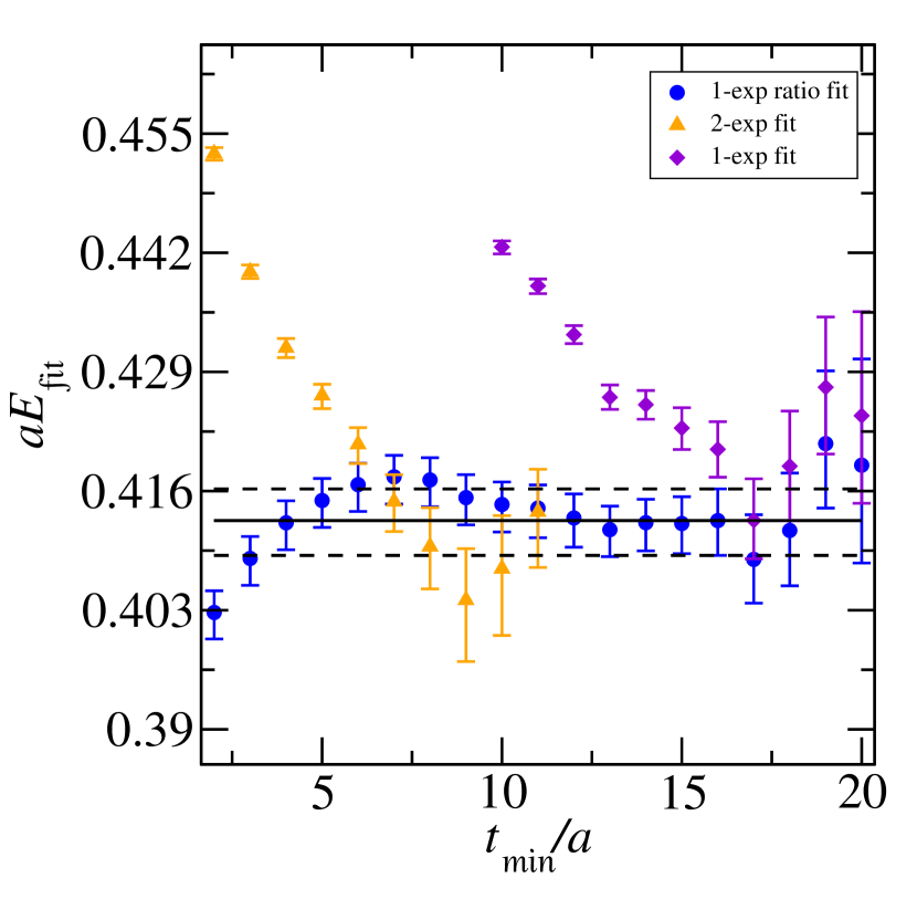
(d) $H_{g}(0)$ level 0

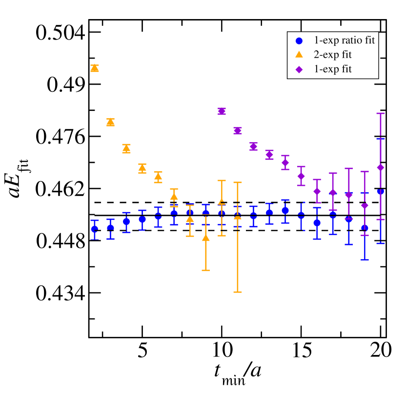
(e) $H_{g}(0)$ level 1

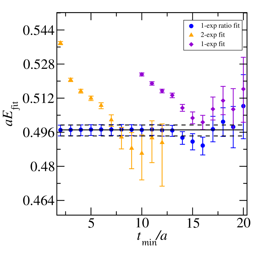
(f) $H_{g}(0)$ level 2

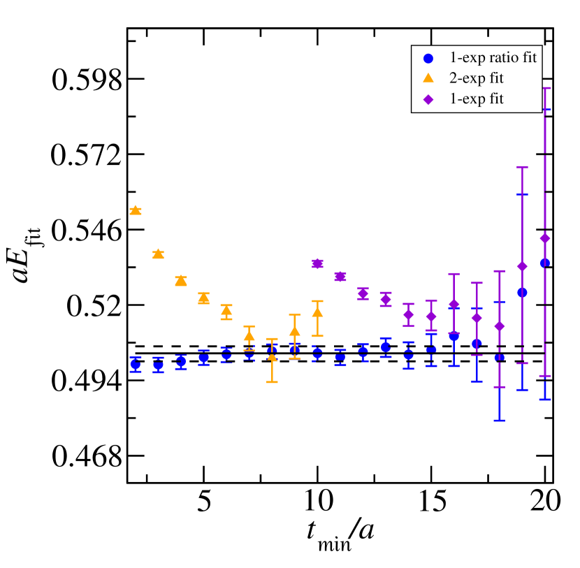
(g) $H_{g}(0)$ level 3

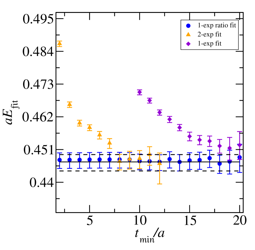
(h) $H_{u}(0)$ level 0

Figure 13: Stability of fits to determine the $I=3/2$ spectrum for total momentum having $\bm{d}^{2}=0$. As in Fig. 11, a variety of fit ranges and fit forms is compared for each level. Each plot contains all fits for a single level in a particular irrep. Indexing for the levels begins at zero for the lowest and increases with increasing energy.

a $G_{1}(1)$ level 0

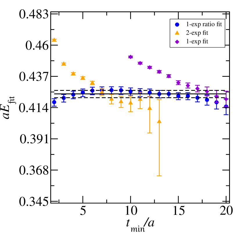
b $G_{1}(1)$ level 1

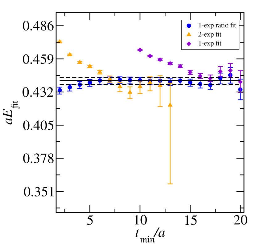
c $G_{1}(1)$ level 2

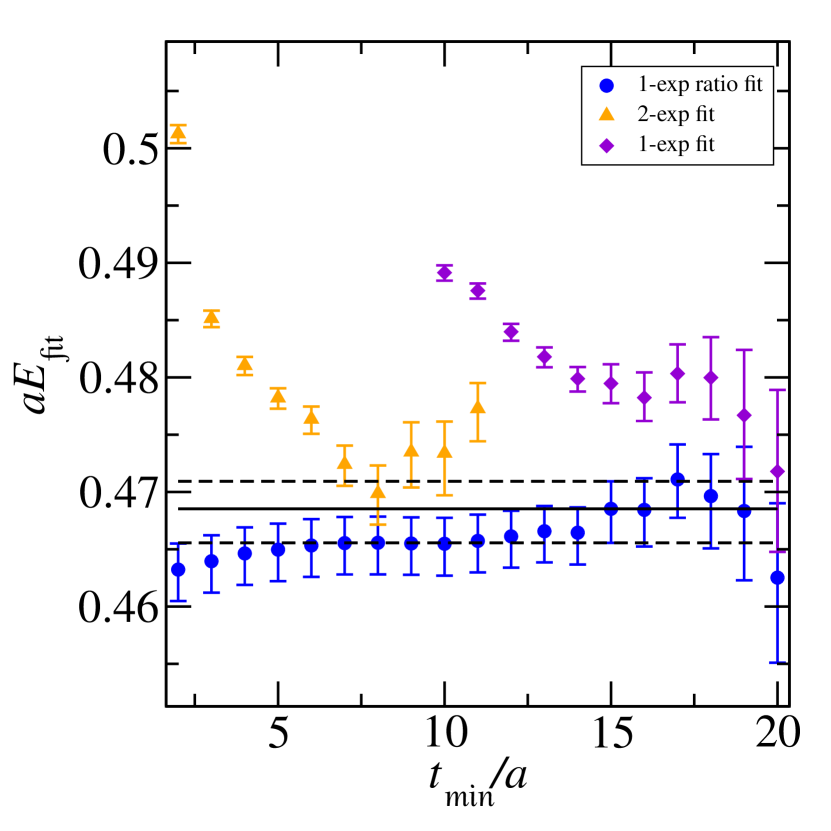
d $G_{1}(1)$ level 3

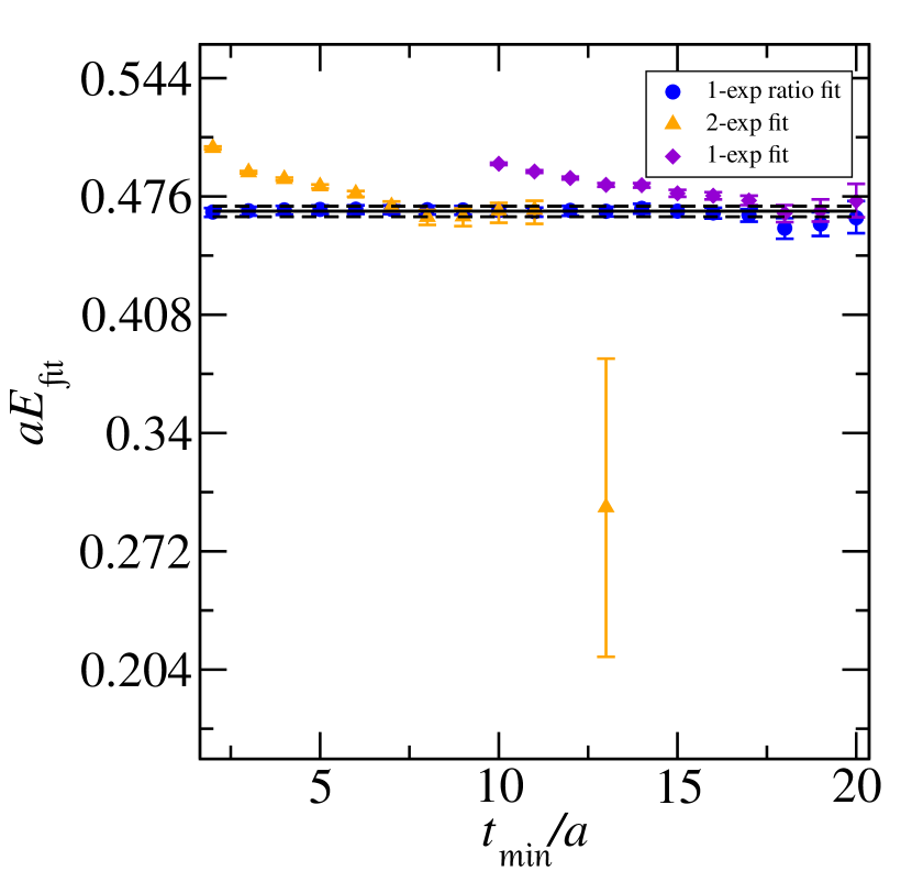
e $G_{1}(1)$ level 4

f $G_{1}(1)$ level 5

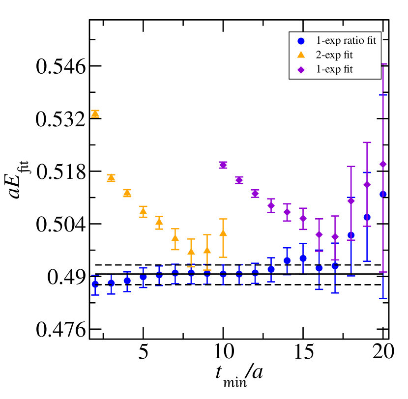
g $G_{1}(1)$ level 6

h $G_{2}(1)$ level 0

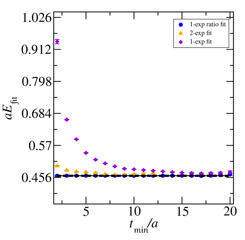
i $G_{2}(1)$ level 1

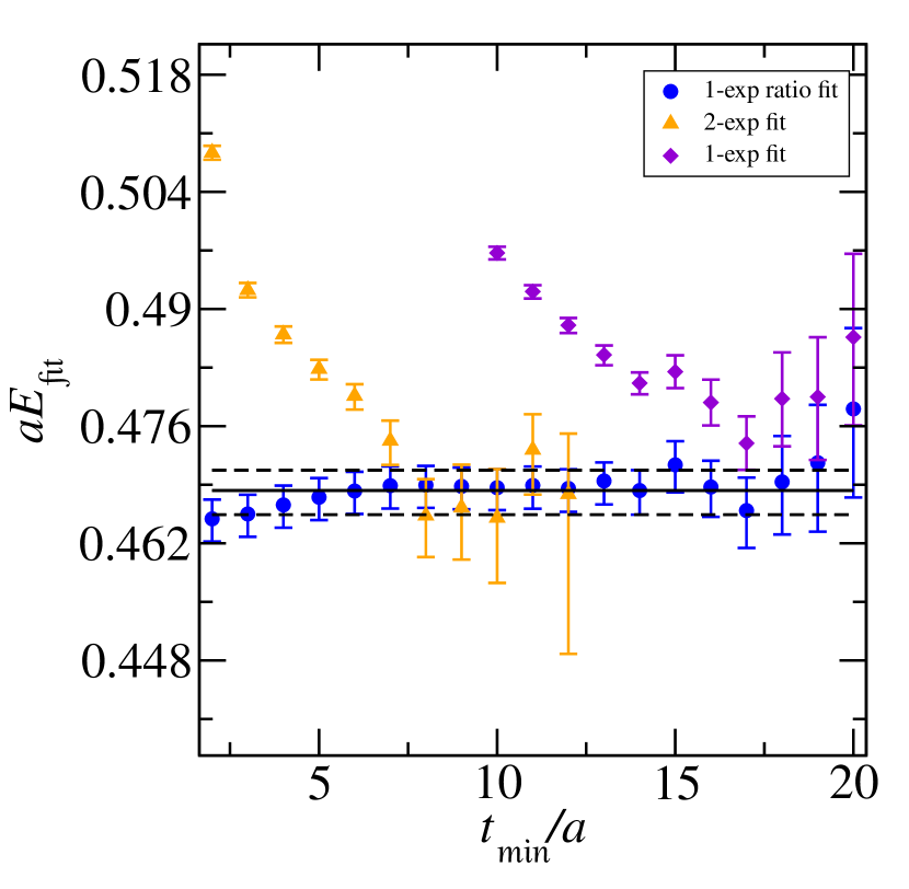
j $G_{2}(1)$ level 2

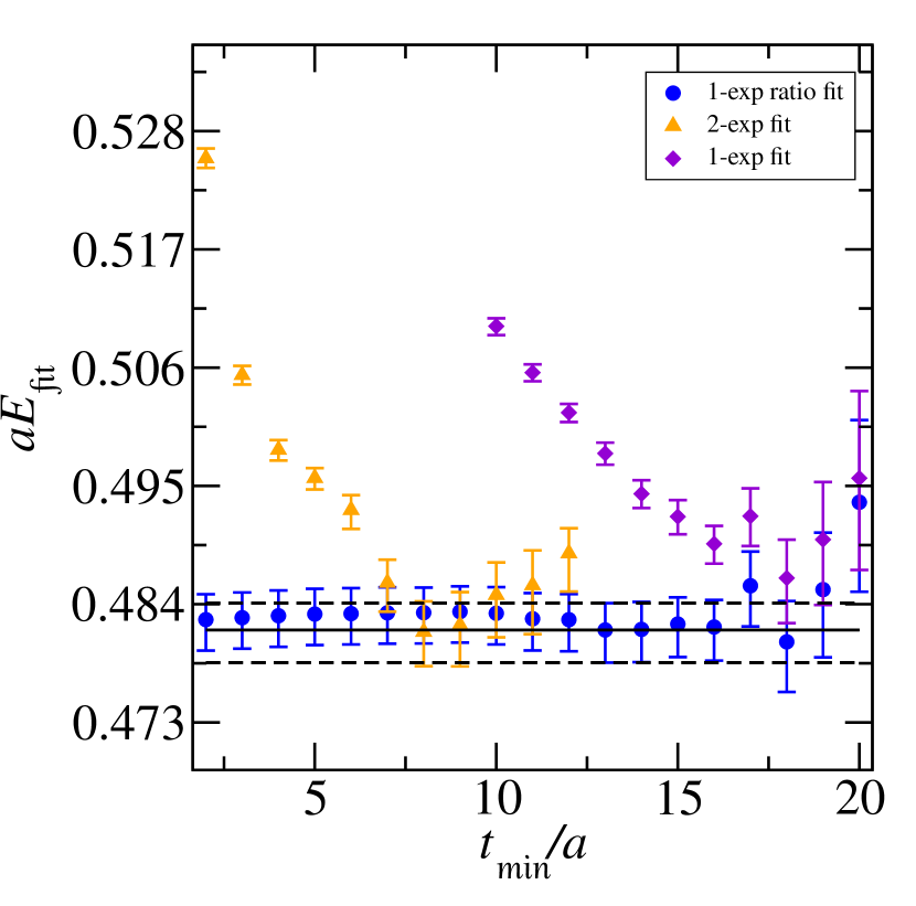
k $G_{2}(1)$ level 3

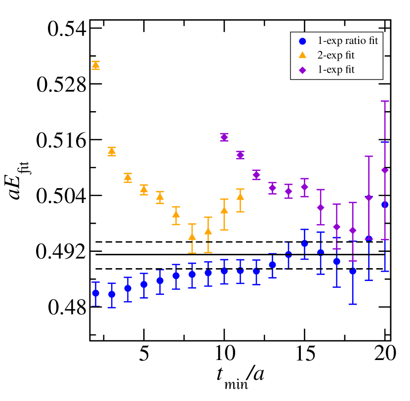
l $G_{2}(1)$ level 4

Figure 15: Same as Fig. 13 for $I=3/2$ except that $\bm{d}^{2}=1$.

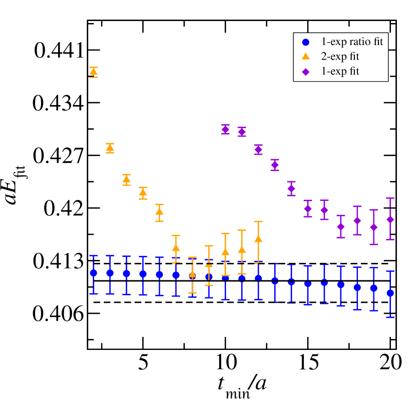
a $G(2)$ level 0

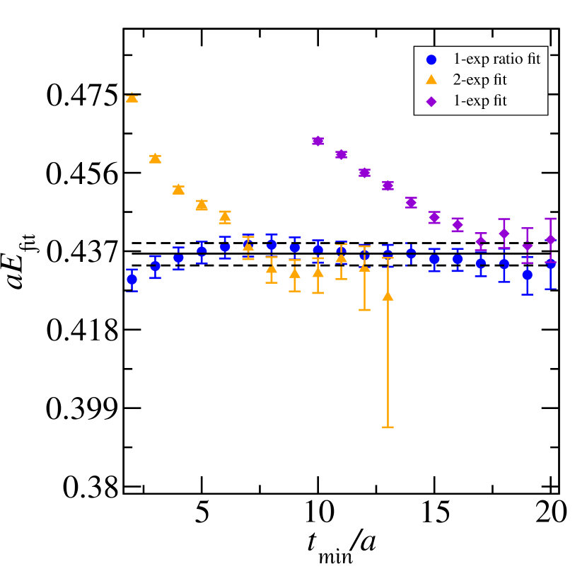
b $G(2)$ level 1

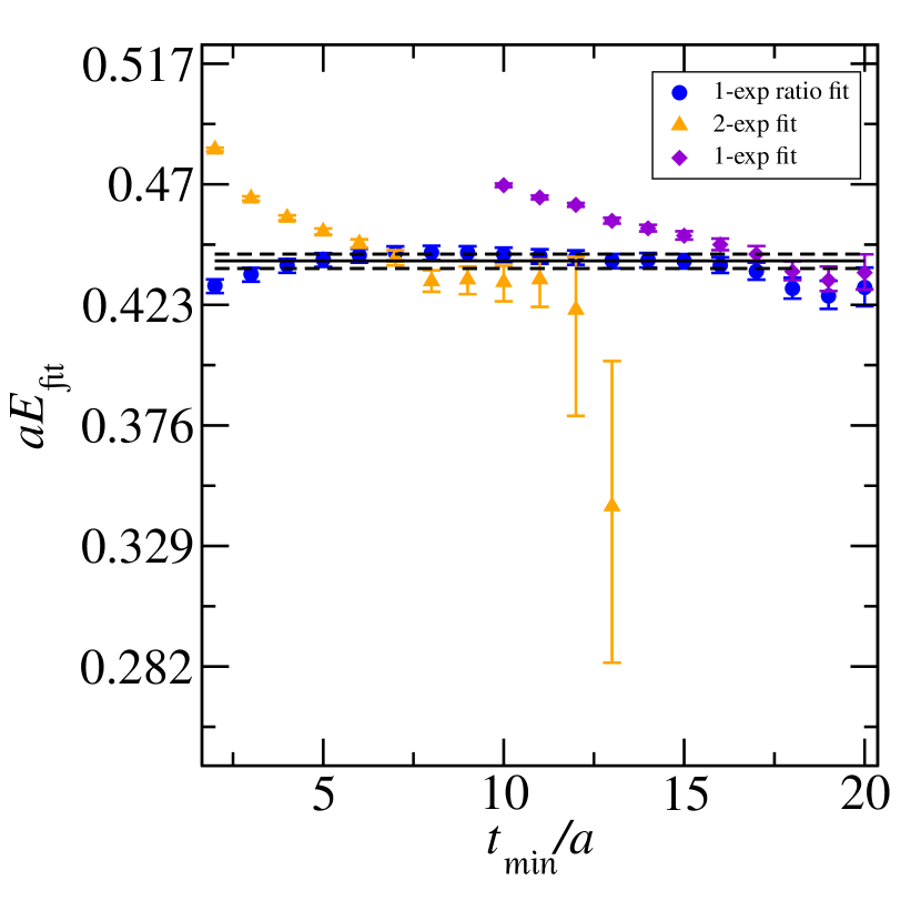
c $G(2)$ level 2

d $G(2)$ level 3

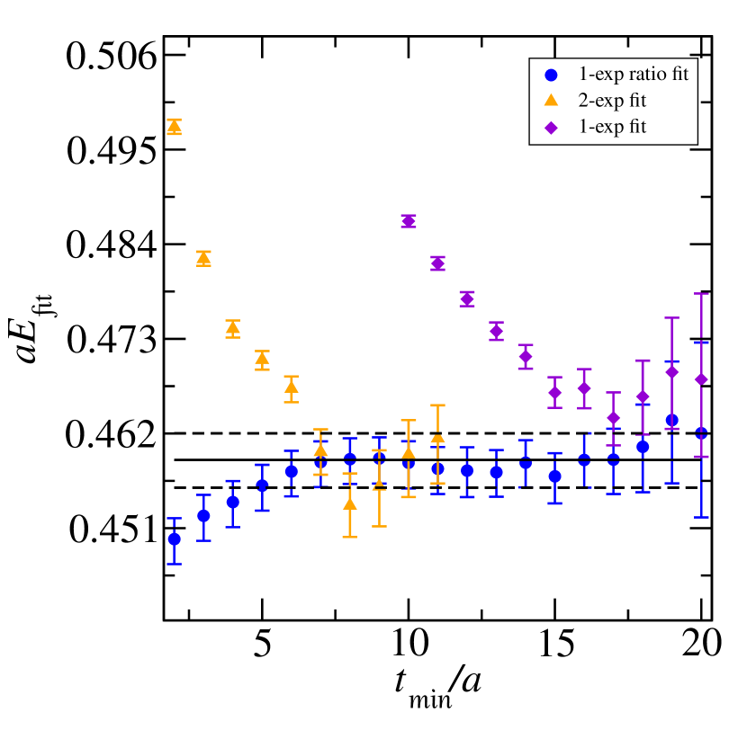
e $G(2)$ level 4

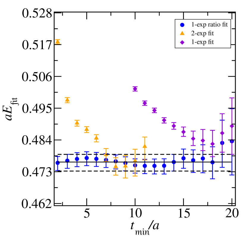
f $G(2)$ level 5

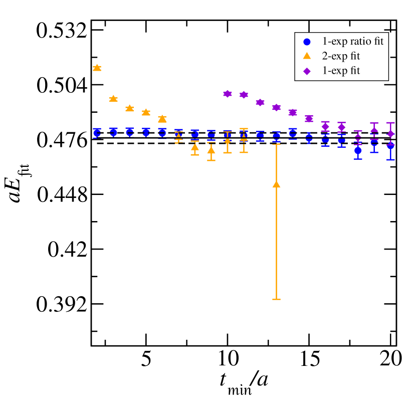
g $G(2)$ level 6

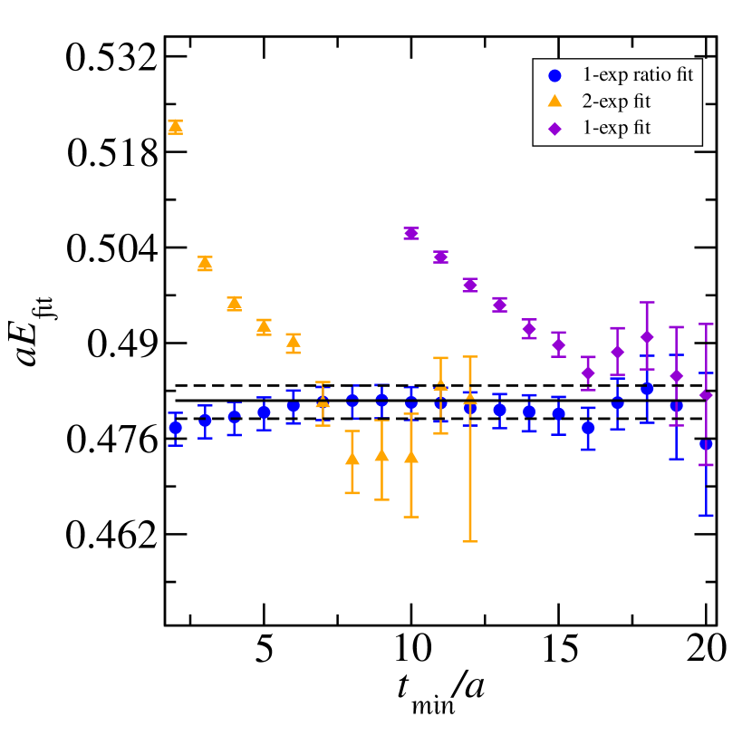
h $G(2)$ level 7

Figure 17: Same as Fig. 13 for $I=3/2$ except that $\bm{d}^{2}=2$.

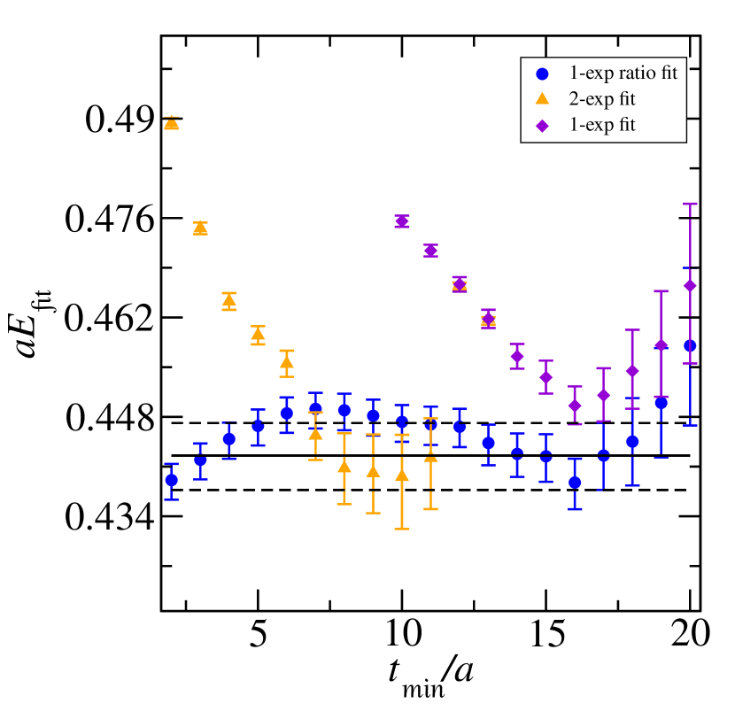
a $F_{1}(3)$ level 0

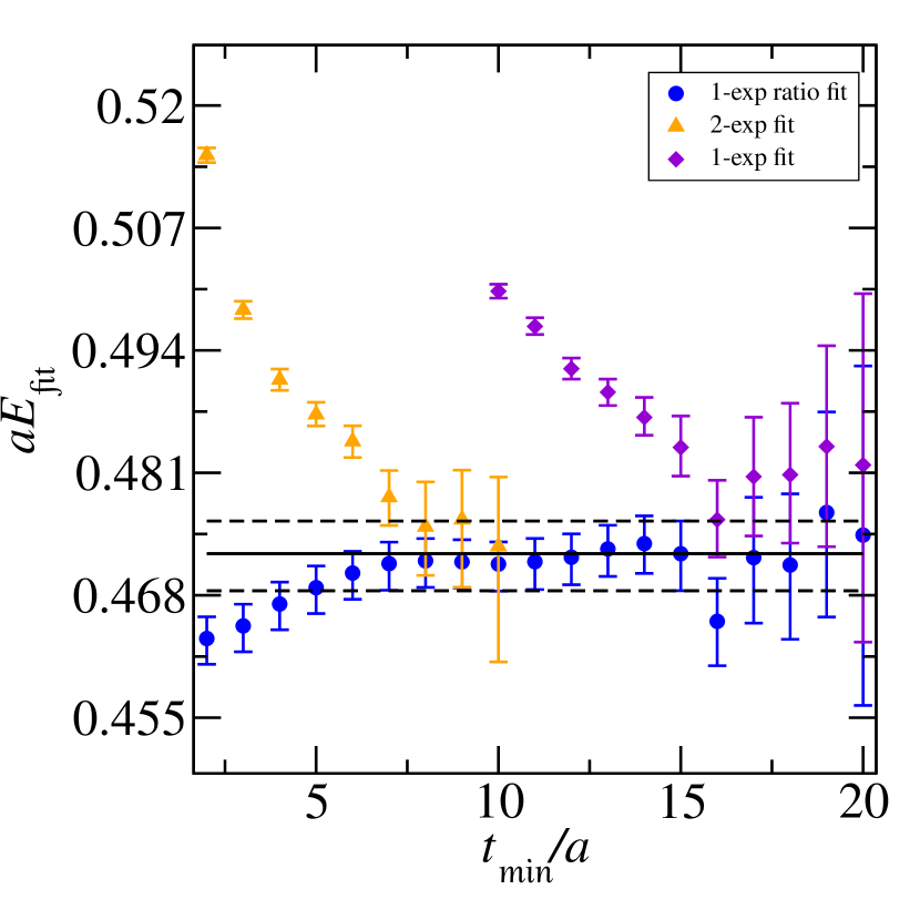
b $F_{1}(3)$ level 1

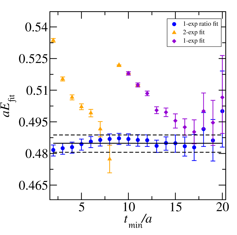
c $F_{1}(3)$ level 2

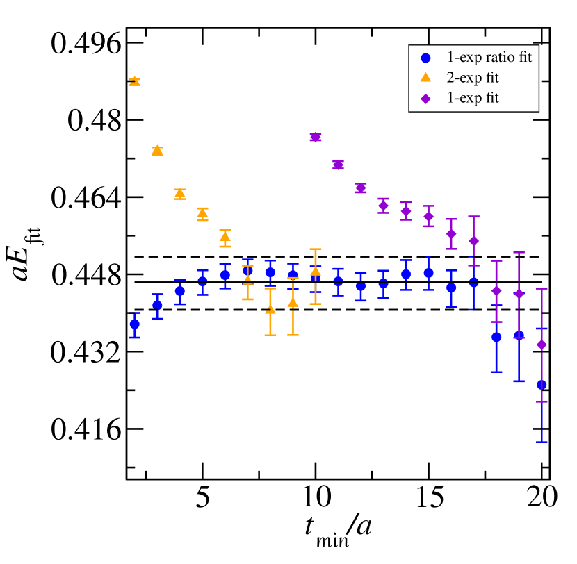
d $F_{2}(3)$ level 0

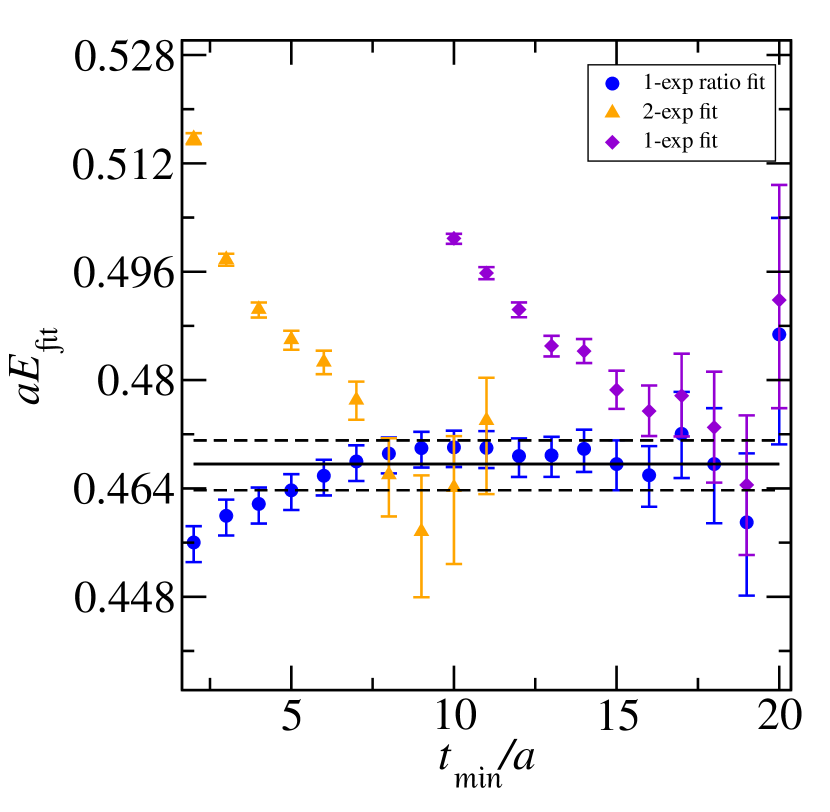
e $F_{2}(3)$ level 1

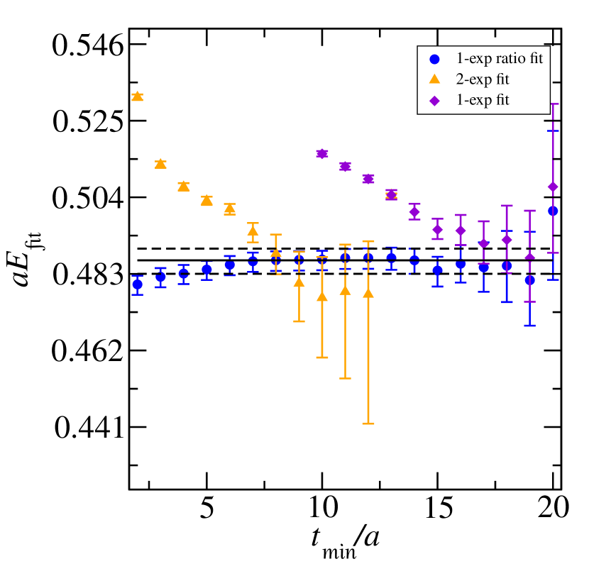
f $F_{2}(3)$ level 2

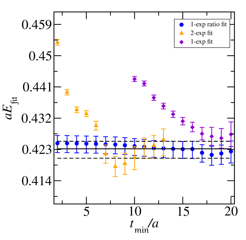
g $G(3)$ level 0

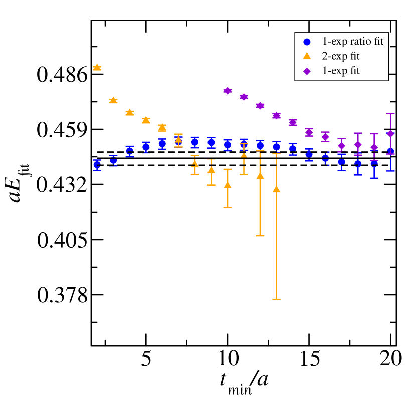
h $G(3)$ level 1

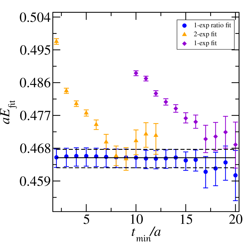
i $G(3)$ level 2

j $G(3)$ level 3

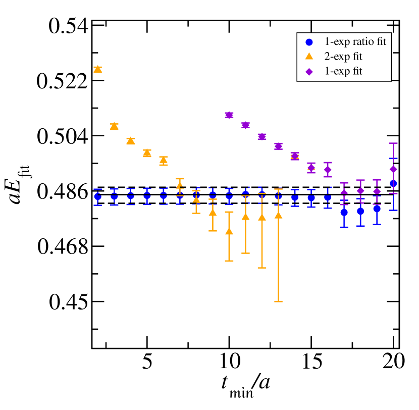
k $G(3)$ level 4

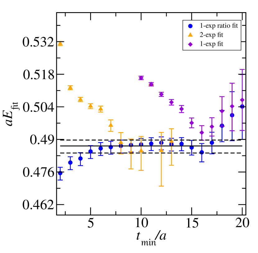
l $G(3)$ level 5

Figure 19: Same as Fig. 13 for $I=3/2$ except that $\bm{d}^{2}=3$.

a $G_{1}(4)$ level 0

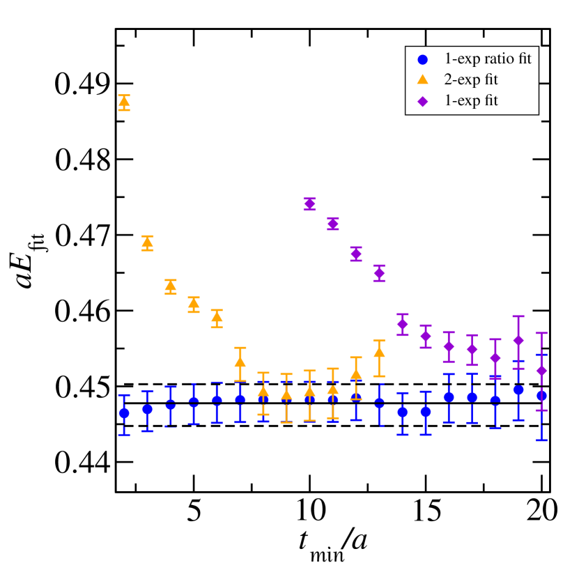
b $G_{1}(4)$ level 1

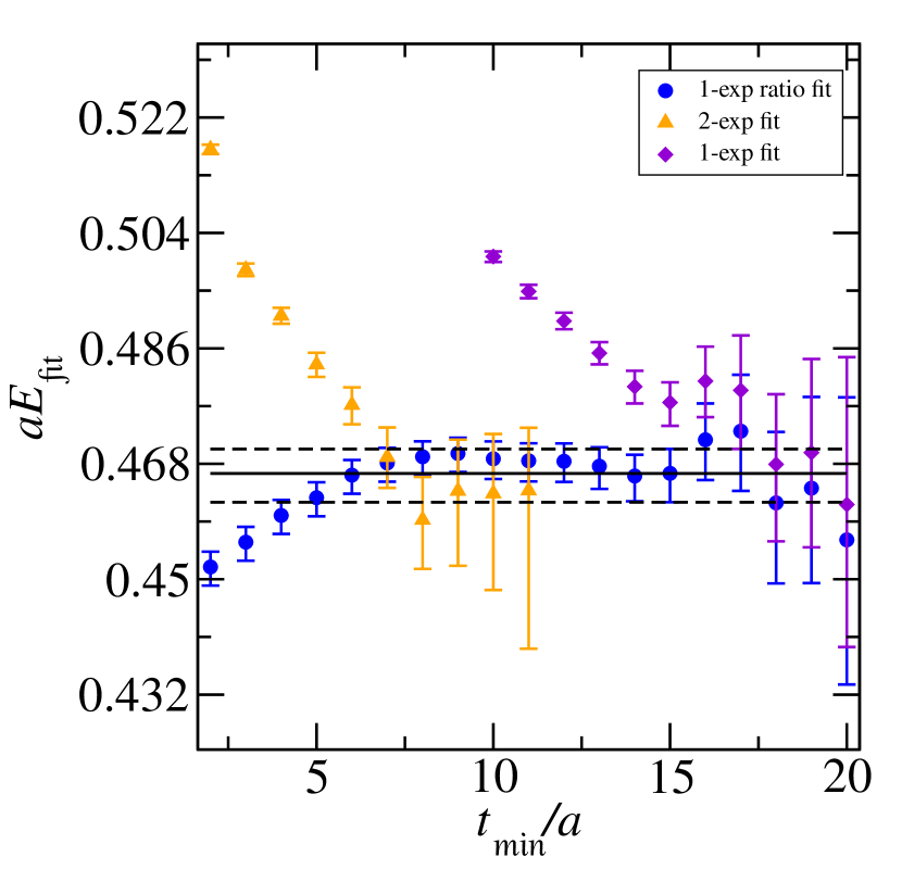
c $G_{1}(4)$ level 2

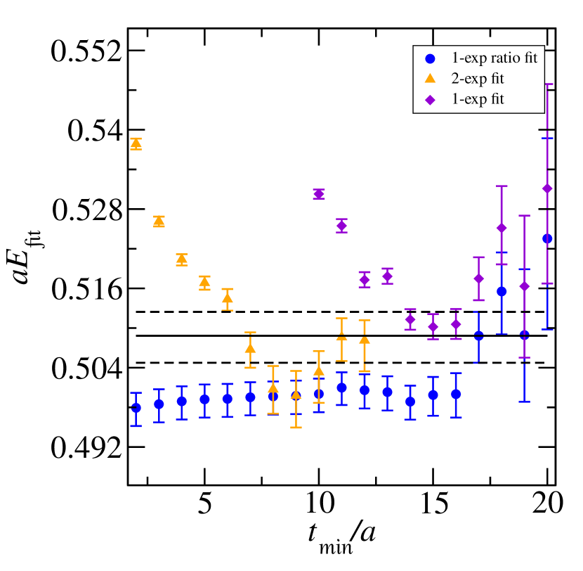
d $G_{1}(4)$ level 3

e $G_{1}(4)$ level 4

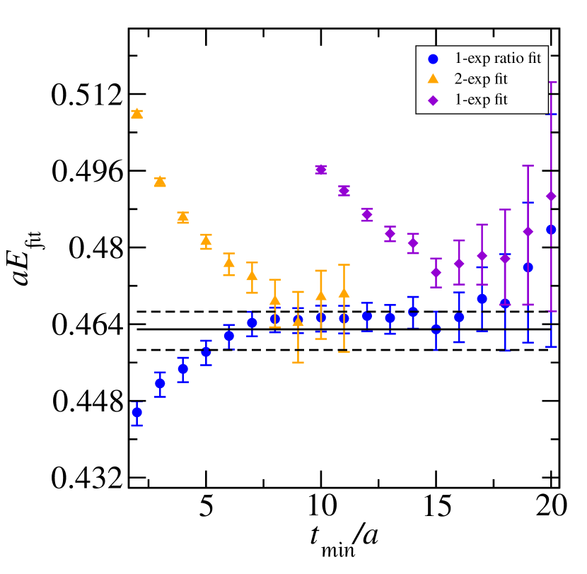
f $G_{2}(4)$ level 0

g $G_{2}(4)$ level 1

h $G_{2}(4)$ level 2

Figure 21: Same as Fig. 13 for $I=3/2$ except that $\bm{d}^{2}=4$.

References

- [1] J. Ruiz de Elvira, M. Hoferichter, B. Kubis, U.G. Meißner, Extracting the -term from low-energy pion-nucleon scattering, J. Phys. G 45 (2018) 024001. arXiv:1706.01465, doi:10.1088/1361-6471/aa9422.
- [2] J. Gasser, H. Leutwyler, Chiral Perturbation Theory to One Loop, Annals Phys. 158 (1984) 142. doi:10.1016/0003-4916(84)90242-2.
- [3] S. Weinberg, Nuclear forces from chiral Lagrangians, Phys. Lett. B 251 (1990) 288–292. doi:10.1016/0370-2693(90)90938-3.
- [4] S. Weinberg, Effective chiral Lagrangians for nucleon - pion interactions and nuclear forces, Nucl. Phys. B 363 (1991) 3–18. doi:10.1016/0550-3213(91)90231-L.
- [5] H. W. Hammer, S. König, U. van Kolck, Nuclear effective field theory: status and perspectives, Rev. Mod. Phys. 92 (2020) 025004. arXiv:1906.12122, doi:10.1103/RevModPhys.92.025004.
- [6] C. Drischler, W. Haxton, K. McElvain, E. Mereghetti, A. Nicholson, P. Vranas, A. Walker-Loud, Towards grounding nuclear physics in QCD, Prog. Part. Nucl. Phys. 121 (2021) 103888. arXiv:1910.07961, doi:10.1016/j.ppnp.2021.103888.
- [7] I. Tews, Z. Davoudi, A. Ekström, J. D. Holt, J. E. Lynn, New Ideas in Constraining Nuclear Forces, J. Phys. G 47 (2020) 103001. arXiv:2001.03334, doi:10.1088/1361-6471/ab9079.
- [8] Z. Davoudi, W. Detmold, K. Orginos, A. Parreño, M. J. Savage, P. Shanahan, M. L. Wagman, Nuclear matrix elements from lattice QCD for electroweak and beyond-Standard-Model processes, Phys. Rept. 900 (2021) 1–74. arXiv:2008.11160, doi:10.1016/j.physrep.2020.10.004.
- [9] V. Cirigliano, et al., Neutrinoless Double-Beta Decay: A Roadmap for Matching Theory to Experiment arXiv:2203.12169.
- [10] V. Cirigliano, et al., Towards precise and accurate calculations of neutrinoless double-beta decay, J. Phys. G 49 (2022) 120502. arXiv:2207.01085, doi:10.1088/1361-6471/aca03e.
- [11] M. Niehus, M. Hoferichter, B. Kubis, J. Ruiz de Elvira, Two-Loop Analysis of the Pion Mass Dependence of the Meson, Phys. Rev. Lett. 126 (2021) 102002. arXiv:2009.04479, doi:10.1103/PhysRevLett.126.102002.
- [12] R. Molina, J. Ruiz de Elvira, Light- and strange-quark mass dependence of the (770) meson revisited, JHEP 11 (2020) 017. arXiv:2005.13584, doi:10.1007/JHEP11(2020)017.
- [13] M. Mai, C. Culver, A. Alexandru, M. Döring, F. X. Lee, Cross-channel study of pion scattering from lattice QCD, Phys. Rev. D 100 (2019) 114514. arXiv:1908.01847, doi:10.1103/PhysRevD.100.114514.
- [14] X.Y. Guo, M. F. M. Lutz, On light vector mesons and chiral SU(3) extrapolations, Nucl. Phys. A 988 (2019) 48–58. arXiv:1810.07078, doi:10.1016/j.nuclphysa.2019.02.007.
- [15] X.Y. Guo, Y. Heo, M. F. M. Lutz, On chiral extrapolations of charmed meson masses and coupled-channel reaction dynamics, Phys. Rev. D 98 (2018) 014510. arXiv:1801.10122, doi:10.1103/PhysRevD.98.014510.
- [16] D. R. Bolton, R. A. Briceno, D. J. Wilson, Connecting physical resonant amplitudes and lattice QCD, Phys. Lett. B757 (2016) 50–56. arXiv:1507.07928, doi:10.1016/j.physletb.2016.03.043.
- [17] A. Walker-Loud, et al., Light hadron spectroscopy using domain wall valence quarks on an Asqtad sea, Phys. Rev. D 79 (2009) 054502. arXiv:0806.4549, doi:10.1103/PhysRevD.79.054502.
- [18] A. Walker-Loud, Baryons in/and Lattice QCD, PoS CD12 (2013) 017. arXiv:1304.6341, doi:10.22323/1.172.0017.
- [19] C. C. Chang, et al., A per-cent-level determination of the nucleon axial coupling from quantum chromodynamics, Nature 558 (2018) 91–94. arXiv:1805.12130, doi:10.1038/s41586-018-0161-8.
- [20] D. Siemens, J. Ruiz de Elvira, E. Epelbaum, M. Hoferichter, H. Krebs, B. Kubis, U. G. Meißner, Reconciling threshold and subthreshold expansions for pion–nucleon scattering, Phys. Lett. B 770 (2017) 27–34. arXiv:1610.08978, doi:10.1016/j.physletb.2017.04.039.
- [21] R. Horsley, Y. Nakamura, H. Perlt, D. Pleiter, P. E. L. Rakow, G. Schierholz, A. Schiller, H. Stuben, F. Winter, J. M. Zanotti, Hyperon sigma terms for 2+1 quark flavours, Phys. Rev. D 85 (2012) 034506. arXiv:1110.4971, doi:10.1103/PhysRevD.85.034506.
- [22] Y.B. Yang, A. Alexandru, T. Draper, J. Liang, K.-F. Liu, N and strangeness sigma terms at the physical point with chiral fermions, Phys. Rev. D 94 (2016) 054503. arXiv:1511.09089, doi:10.1103/PhysRevD.94.054503.
- [23] C. Alexandrou, S. Bacchio, M. Constantinou, J. Finkenrath, K. Hadjiyiannakou, K. Jansen, G. Koutsou, A. Vaquero Aviles-Casco, Nucleon axial, tensor, and scalar charges and -terms in lattice QCD, Phys. Rev. D 102 (2020) 054517. arXiv:1909.00485, doi:10.1103/PhysRevD.102.054517.
- [24] S. Borsanyi, Z. Fodor, C. Hoelbling, L. Lellouch, K. K. Szabo, C. Torrero, L. Varnhorst, Ab-initio calculation of the proton and the neutron’s scalar couplings for new physics searches arXiv:2007.03319.
- [25] M. Hoferichter, J. Ruiz de Elvira, B. Kubis, U.G. Meißner, High-Precision Determination of the Pion-Nucleon Term from Roy-Steiner Equations, Phys. Rev. Lett. 115 (2015) 092301. arXiv:1506.04142, doi:10.1103/PhysRevLett.115.092301.
- [26] R. Gupta, S. Park, M. Hoferichter, E. Mereghetti, B. Yoon, T. Bhattacharya, Pion–Nucleon Sigma Term from Lattice QCD, Phys. Rev. Lett. 127 (2021) 242002. arXiv:2105.12095, doi:10.1103/PhysRevLett.127.242002.
- [27] M. Hoferichter, J. Ruiz de Elvira, B. Kubis, U.G. Meißner, Remarks on the pion–nucleon -term, Phys. Lett. B 760 (2016) 74–78. arXiv:1602.07688, doi:10.1016/j.physletb.2016.06.038.
- [28] B. Abi, et al., Deep Underground Neutrino Experiment (DUNE), Far Detector Technical Design Report, Volume I Introduction to DUNE, JINST 15 (2020) T08008. arXiv:2002.02967, doi:10.1088/1748-0221/15/08/T08008.
- [29] K. Abe, et al., Hyper-kamiokande design reportarXiv:1805.04163.
- [30] A. S. Meyer, A. Walker-Loud, C. Wilkinson, Status of Lattice QCD Determination of Nucleon Form Factors and their Relevance for the Few-GeV Neutrino Program, Annual Review of Nuclear and Particle Science 72 (2022) 205. arXiv:2201.01839, doi:10.1146/annurev-nucl-010622-120608.
- [31] R. A. Briceno, J. J. Dudek, R. D. Young, Scattering processes and resonances from lattice QCD, Rev. Mod. Phys. 90 (2018) 025001. arXiv:1706.06223, doi:10.1103/RevModPhys.90.025001.
- [32] B. Hörz, A. Hanlon, Two- and three-pion finite-volume spectra at maximal isospin from lattice QCD, Phys. Rev. Lett. 123 (2019) 142002. arXiv:1905.04277, doi:10.1103/PhysRevLett.123.142002.
- [33] T. D. Blanton, F. Romero-López, S. R. Sharpe, Three-Pion Scattering Amplitude from Lattice QCD, Phys. Rev. Lett. 124 (2020) 032001. arXiv:1909.02973, doi:10.1103/PhysRevLett.124.032001.
- [34] M. T. Hansen, R. A. Briceño, R. G. Edwards, C. E. Thomas, D. J. Wilson, Energy-Dependent Scattering Amplitude from QCD, Phys. Rev. Lett. 126 (2021) 012001. arXiv:2009.04931, doi:10.1103/PhysRevLett.126.012001.
- [35] M. Fischer, B. Kostrzewa, L. Liu, F. Romero-López, M. Ueding, C. Urbach, Scattering of two and three physical pions at maximal isospin from lattice QCD, Eur. Phys. J. C 81 (2021) 436. arXiv:2008.03035, doi:10.1140/epjc/s10052-021-09206-5.
- [36] A. Alexandru, R. Brett, C. Culver, M. Döring, D. Guo, F. X. Lee, M. Mai, Finite-volume energy spectrum of the system, Phys. Rev. D 102 (2020) 114523. arXiv:2009.12358, doi:10.1103/PhysRevD.102.114523.
- [37] T. D. Blanton, A. D. Hanlon, B. Hörz, C. Morningstar, F. Romero-López, S. R. Sharpe, Interactions of two and three mesons including higher partial waves from lattice QCD, JHEP 10 (2021) 023. arXiv:2106.05590, doi:10.1007/JHEP10(2021)023.
- [38] M. Mai, A. Alexandru, R. Brett, C. Culver, M. Döring, F. X. Lee, D. Sadasivan, Three-Body Dynamics of the a1(1260) Resonance from Lattice QCD, Phys. Rev. Lett. 127 (2021) 222001. arXiv:2107.03973, doi:10.1103/PhysRevLett.127.222001.
- [39] C. Lang, V. Verduci, Scattering in the negative parity channel in lattice QCD, Phys.Rev. D87 (2013) 054502. arXiv:1212.5055, doi:10.1103/PhysRevD.87.054502.
- [40] C. W. Andersen, J. Bulava, B. Hörz, C. Morningstar, Elastic , -wave nucleon-pion scattering amplitude and the (1232) resonance from Nf=2+1 lattice QCD, Phys. Rev. D97 (2018) 014506. arXiv:1710.01557, doi:10.1103/PhysRevD.97.014506.
- [41] C. Alexandrou, L. Leskovec, S. Meinel, J. Negele, S. Paul, M. Petschlies, A. Pochinsky, G. Rendon, S. Syritsyn, -wave scattering and the resonance from lattice QCD, Phys. Rev. D96 (2017) 034525. arXiv:1704.05439, doi:10.1103/PhysRevD.96.034525.
- [42] M. Fukugita, Y. Kuramashi, M. Okawa, H. Mino, A. Ukawa, Hadron scattering lengths in lattice QCD, Phys. Rev. D52 (1995) 3003–3023. arXiv:hep-lat/9501024, doi:10.1103/PhysRevD.52.3003.
-
[43]
V. Verduci,
Pion-nucleon
scattering in lattice QCD, Ph.D. thesis, Graz U. (2014).
URL http://unipub.uni-graz.at/obvugrhs/content/titleinfo/252105 - [44] D. Mohler, Review of lattice studies of resonances, PoS LATTICE2012 (2012) 003. arXiv:1211.6163.
- [45] F. Pittler, C. Alexandrou, K. Hadjiannakou, G. Koutsou, S. Paul, M. Petschlies, A. Todaro, Elastic scattering in the I = 3/2 channel, PoS LATTICE2021 (2022) 226. arXiv:2112.04146, doi:10.22323/1.396.0226.
- [46] C. B. Lang, L. Leskovec, M. Padmanath, S. Prelovsek, Pion-nucleon scattering in the Roper channel from lattice QCD, Phys. Rev. D95 (2017) 014510. arXiv:1610.01422, doi:10.1103/PhysRevD.95.014510.
- [47] W. Detmold, A. Nicholson, Low energy scattering phase shifts for meson-baryon systems, Phys. Rev. D93 (2016) 114511. arXiv:1511.02275, doi:10.1103/PhysRevD.93.114511.
- [48] A. Torok, S. R. Beane, W. Detmold, T. C. Luu, K. Orginos, A. Parreno, M. J. Savage, A. Walker-Loud, Meson-Baryon Scattering Lengths from Mixed-Action Lattice QCD, Phys. Rev. D81 (2010) 074506. arXiv:0907.1913, doi:10.1103/PhysRevD.81.074506.
- [49] M. Peardon, J. Bulava, J. Foley, C. Morningstar, J. Dudek, R. G. Edwards, B. Joo, H.-W. Lin, D. G. Richards, K. J. Juge, A Novel quark-field creation operator construction for hadronic physics in lattice QCD, Phys. Rev. D80 (2009) 054506. arXiv:0905.2160, doi:10.1103/PhysRevD.80.054506.
- [50] C. Morningstar, J. Bulava, J. Foley, K. J. Juge, D. Lenkner, M. Peardon, C. H. Wong, Improved stochastic estimation of quark propagation with Laplacian Heaviside smearing in lattice QCD, Phys. Rev. D83 (2011) 114505. arXiv:1104.3870, doi:10.1103/PhysRevD.83.114505.
- [51] T. D. Blanton, F. Romero-López, S. R. Sharpe, Implementing the three-particle quantization condition including higher partial waves, JHEP 03 (2019) 106. arXiv:1901.07095, doi:10.1007/JHEP03(2019)106.
- [52] C. Culver, M. Mai, R. Brett, A. Alexandru, M. Döring, Three pion spectrum in the channel from lattice QCD, Phys. Rev. D 101 (2020) 114507. arXiv:1911.09047, doi:10.1103/PhysRevD.101.114507.
- [53] R. Brett, C. Culver, M. Mai, A. Alexandru, M. Döring, F. X. Lee, Three-body interactions from the finite-volume QCD spectrum, Phys. Rev. D 104 (2021) 014501. arXiv:2101.06144, doi:10.1103/PhysRevD.104.014501.
- [54] A. Francis, J. R. Green, P. M. Junnarkar, C. Miao, T. D. Rae, H. Wittig, Lattice QCD study of the dibaryon using hexaquark and two-baryon interpolators, Phys. Rev. D 99 (7) (2019) 074505. arXiv:1805.03966, doi:10.1103/PhysRevD.99.074505.
- [55] J. R. Green, A. D. Hanlon, P. M. Junnarkar, H. Wittig, Weakly Bound H Dibaryon from SU(3)-Flavor-Symmetric QCD, Phys. Rev. Lett. 127 (2021) 242003. arXiv:2103.01054, doi:10.1103/PhysRevLett.127.242003.
- [56] B. Hörz, et al., Two-nucleon S-wave interactions at the flavor-symmetric point with : A first lattice QCD calculation with the stochastic Laplacian Heaviside method, Phys. Rev. C 103 (2021) 014003. arXiv:2009.11825, doi:10.1103/PhysRevC.103.014003.
- [57] C. Morningstar, J. Bulava, B. Singha, R. Brett, J. Fallica, A. Hanlon, B. Hörz, Estimating the two-particle -matrix for multiple partial waves and decay channels from finite-volume energies, Nucl. Phys. B924 (2017) 477–507. arXiv:1707.05817, doi:10.1016/j.nuclphysb.2017.09.014.
- [58] D. Mohler, S. Schaefer, Remarks on strange-quark simulations with Wilson fermions, Phys. Rev. D 102 (2020) 074506. arXiv:2003.13359, doi:10.1103/PhysRevD.102.074506.
- [59] L. Maiani, M. Testa, Final state interactions from Euclidean correlation functions, Phys. Lett. B245 (1990) 585–590. doi:10.1016/0370-2693(90)90695-3.
- [60] M. Lüscher, Two particle states on a torus and their relation to the scattering matrix, Nucl. Phys. B354 (1991) 531–578. doi:10.1016/0550-3213(91)90366-6.
- [61] M. Bruno, M. T. Hansen, Variations on the Maiani-Testa approach and the inverse problem, JHEP 06 (2021) 043. arXiv:2012.11488, doi:10.1007/JHEP06(2021)043.
- [62] M. T. Hansen, H. B. Meyer, D. Robaina, From deep inelastic scattering to heavy-flavor semileptonic decays: Total rates into multihadron final states from lattice QCD, Phys. Rev. D96 (2017) 094513. arXiv:1704.08993, doi:10.1103/PhysRevD.96.094513.
- [63] J. Bulava, M. T. Hansen, Scattering amplitudes from finite-volume spectral functions, Phys. Rev. D 100 (2019) 034521. arXiv:1903.11735, doi:10.1103/PhysRevD.100.034521.
- [64] J. C. A. Barata, K. Fredenhagen, Particle scattering in Euclidean lattice field theories, Commun. Math. Phys. 138 (1991) 507–520. doi:10.1007/BF02102039.
- [65] M. Göckeler, R. Horsley, M. Lage, U. G. Meißner, P. E. L. Rakow, A. Rusetsky, G. Schierholz, J. M. Zanotti, Scattering phases for meson and baryon resonances on general moving-frame lattices, Phys. Rev. D86 (2012) 094513. arXiv:1206.4141, doi:10.1103/PhysRevD.86.094513.
- [66] M. Bruno, et al., Simulation of QCD with N 2 1 flavors of non-perturbatively improved Wilson fermions, JHEP 02 (2015) 043. arXiv:1411.3982, doi:10.1007/JHEP02(2015)043.
- [67] M. Luscher, P. Weisz, On-Shell Improved Lattice Gauge Theories, Commun. Math. Phys. 97 (1985) 59, [Erratum: Commun. Math. Phys.98,433(1985)]. doi:10.1007/BF01206178.
- [68] J. Bulava, S. Schaefer, Improvement of lattice QCD with Wilson fermions and tree-level improved gauge action, Nucl. Phys. B874 (2013) 188–197. arXiv:1304.7093, doi:10.1016/j.nuclphysb.2013.05.019.
- [69] M. Lüscher, S. Schaefer, Lattice QCD without topology barriers, JHEP 07 (2011) 036. arXiv:1105.4749, doi:10.1007/JHEP07(2011)036.
- [70] C. Andersen, J. Bulava, B. Hörz, C. Morningstar, The pion-pion scattering amplitude and timelike pion form factor from lattice QCD, Nucl. Phys. B939 (2019) 145–173. arXiv:1808.05007, doi:10.1016/j.nuclphysb.2018.12.018.
- [71] M. Lüscher, F. Palombi, Fluctuations and reweighting of the quark determinant on large lattices, PoS LATTICE2008 (2008) 049. arXiv:0810.0946.
- [72] M. A. Clark, A. D. Kennedy, Accelerating dynamical fermion computations using the rational hybrid Monte Carlo (RHMC) algorithm with multiple pseudofermion fields, Phys. Rev. Lett. 98 (2007) 051601. arXiv:hep-lat/0608015, doi:10.1103/PhysRevLett.98.051601.
- [73] M. Bruno, T. Korzec, S. Schaefer, Setting the scale for the CLS flavor ensembles, Phys. Rev. D95 (2017) 074504. arXiv:1608.08900, doi:10.1103/PhysRevD.95.074504.
- [74] B. Strassberger, et al., Scale setting for CLS 2+1 simulations, PoS LATTICE2021 (2022) 135. arXiv:2112.06696, doi:10.22323/1.396.0135.
- [75] C. Morningstar, J. Bulava, B. Fahy, J. Foley, Y. Jhang, et al., Extended hadron and two-hadron operators of definite momentum for spectrum calculations in lattice QCD, Phys.Rev. D88 (2013) 014511. arXiv:1303.6816, doi:10.1103/PhysRevD.88.014511.
- [76] C. Morningstar, M. J. Peardon, Analytic smearing of SU(3) link variables in lattice QCD, Phys. Rev. D69 (2004) 054501. arXiv:hep-lat/0311018, doi:10.1103/PhysRevD.69.054501.
- [77] C. Michael, I. Teasdale, Extracting Glueball Masses From Lattice QCD, Nucl. Phys. B215 (1983) 433. doi:10.1016/0550-3213(83)90674-0.
- [78] M. Luscher, U. Wolff, How to Calculate the Elastic Scattering Matrix in Two-dimensional Quantum Field Theories by Numerical Simulation, Nucl. Phys. B339 (1990) 222–252. doi:10.1016/0550-3213(90)90540-T.
- [79] B. Blossier, M. Della Morte, G. von Hippel, T. Mendes, R. Sommer, On the generalized eigenvalue method for energies and matrix elements in lattice field theory, JHEP 04 (2009) 094. arXiv:0902.1265, doi:10.1088/1126-6708/2009/04/094.
- [80] F. J. Yndurain, R. Garcia-Martin, J. R. Pelaez, Experimental status of the isoscalar S wave at low energy: pole and scattering length, Phys. Rev. D 76 (2007) 074034. arXiv:hep-ph/0701025, doi:10.1103/PhysRevD.76.074034.
- [81] P. Guo, J. Dudek, R. Edwards, A. P. Szczepaniak, Coupled-channel scattering on a torus, Phys. Rev. D 88 (2013) 014501. arXiv:1211.0929, doi:10.1103/PhysRevD.88.014501.
- [82] G. Silvi, S. Paul, C. Alexandrou, S. Krieg, L. Leskovec, S. Meinel, J. Negele, M. Petschlies, A. Pochinsky, G. Rendon, S. Syritsyn, A. Todaro, -wave nucleon-pion scattering amplitude in the (1232) channel from lattice QCD, Physical Review D 103 (2021) 094508. doi:10.1103/physrevd.103.094508.
- [83] V. Baru, C. Hanhart, M. Hoferichter, B. Kubis, A. Nogga, D. R. Phillips, Precision calculation of the deuteron scattering length and its impact on threshold N scattering, Phys. Lett. B 694 (2011) 473–477. arXiv:1003.4444, doi:10.1016/j.physletb.2010.10.028.
- [84] V. Baru, C. Hanhart, M. Hoferichter, B. Kubis, A. Nogga, D. R. Phillips, Precision calculation of threshold scattering, N scattering lengths, and the GMO sum rule, Nucl. Phys. A 872 (2011) 69–116. arXiv:1107.5509, doi:10.1016/j.nuclphysa.2011.09.015.
- [85] D. Gotta, et al., Pionic hydrogen, Lect. Notes Phys. 745 (2008) 165–186. doi:10.1007/978-3-540-75479-4_10.
- [86] T. Strauch, et al., Pionic deuterium, Eur. Phys. J. A 47 (2011) 88. arXiv:1011.2415, doi:10.1140/epja/i2011-11088-1.
- [87] M. Hennebach, et al., Hadronic shift in pionic hydrogen, Eur. Phys. J. A 50 (2014) 190, [Erratum: Eur.Phys.J.A 55, 24 (2019)]. arXiv:1406.6525, doi:10.1140/epja/i2014-14190-x.
- [88] M. Hoferichter, J. Ruiz de Elvira, B. Kubis, U.G. Meißner, Roy–Steiner-equation analysis of pion–nucleon scattering, Phys. Rept. 625 (2016) 1–88. arXiv:1510.06039, doi:10.1016/j.physrep.2016.02.002.
- [89] N. Fettes, U.G. Meißner, S. Steininger, Pion-nucleon scattering in chiral perturbation theory. 1. Isospin symmetric case, Nucl. Phys. A 640 (1998) 199–234. arXiv:hep-ph/9803266, doi:10.1016/S0375-9474(98)00452-7.
- [90] N. Fettes, U.G. Meißner, Pion-nucleon scattering in chiral perturbation theory. 2.: Fourth order calculation, Nucl. Phys. A 676 (2000) 311. arXiv:hep-ph/0002162, doi:10.1016/S0375-9474(00)00199-8.
- [91] T. Becher, H. Leutwyler, Low energy analysis of , JHEP 06 (2001) 017. arXiv:hep-ph/0103263, doi:10.1088/1126-6708/2001/06/017.
- [92] M. Hoferichter, J. Ruiz de Elvira, B. Kubis, U.G. Meißner, Matching pion-nucleon Roy-Steiner equations to chiral perturbation theory, Phys. Rev. Lett. 115 (2015) 192301. arXiv:1507.07552, doi:10.1103/PhysRevLett.115.192301.
- [93] P. A. Zyla, et al., Review of Particle Physics, Progress of Theoretical and Experimental Physics 2020, 083C01. arXiv:https://academic.oup.com/ptep/article-pdf/2020/8/083C01/34673722/ptaa104.pdf, doi:10.1093/ptep/ptaa104.
- [94] T. R. Hemmert, B. R. Holstein, N. C. Mukhopadhyay, , couplings and the quark model, Phys. Rev. D51 (1995) 158–167. arXiv:hep-ph/9409323, doi:10.1103/PhysRevD.51.158.
- [95] N. Fettes, U.G. Meißner, M. Mojzis, S. Steininger, The Chiral effective pion nucleon Lagrangian of order , Annals Phys. 283 (2000) 273–302, [Erratum: Annals Phys. 288, 249–250 (2001)]. arXiv:hep-ph/0001308, doi:10.1006/aphy.2000.6059.
- [96] D. Stanzione, J. West, R. T. Evans, T. Minyard, O. Ghattas, D. K. Panda, Frontera: The Evolution of Leadership Computing at the National Science Foundation, Practice and Experience in Advanced Research Computing (PEARC ’20), (2020).