Counterfactual Fairness Is Basically Demographic Parity

Abstract

Making fair decisions is crucial to ethically implementing machine learning algorithms in social settings. In this work, we consider the celebrated definition of counterfactual fairness. We begin by showing that an algorithm which satisfies counterfactual fairness also satisfies demographic parity, a far simpler fairness constraint. Similarly, we show that all algorithms satisfying demographic parity can be trivially modified to satisfy counterfactual fairness. Together, our results indicate that counterfactual fairness is basically equivalent to demographic parity, which has important implications for the growing body of work on counterfactual fairness. We then validate our theoretical findings empirically, analyzing three existing algorithms for counterfactual fairness against three simple benchmarks. We find that two simple benchmark algorithms outperform all three existing algorithms—in terms of fairness, accuracy, and efficiency—on several data sets. Our analysis leads us to formalize a concrete fairness goal: to preserve the order of individuals within protected groups. We believe transparency around the ordering of individuals within protected groups makes fair algorithms more trustworthy. By design, the two simple benchmark algorithms satisfy this goal while the existing algorithms for counterfactual fairness do not.

Introduction

A pressing challenge in the deployment of algorithms in social settings is the risk of “unfair” decisions with respect to protected attributes like race, gender, religion, sexual-orientation, or age. In this work, we consider the supervised learning problem of predicting outcomes from labelled observations where the existing outcomes are already biased. The observations consist of protected attributes and other remaining attributes like test scores, grade point averages, credit scores, health risks, and more context dependent variables. The goal is to “fairly” predict outcomes like student success, credit worthiness, and health care needs.

One approach is to ignore the protected attributes and train algorithms only on the remaining attributes i.e. “fairness through blindness” (Dwork et al. 2012). However, there could be variables like height or zip code which are proxies for protected attributes (Pedreshi, Ruggieri, and Turini 2008; Corbett-Davies and Goel 2018). Even in the absence of these proxy variables, seemingly reasonable remaining predictive attributes like study time or prior health care can still depend on protected attributes. A natural consequentialist approach in the face of concerns over group equity is demographic parity, which ensures an identical distribution over the outcomes for each protected group. However, demographic parity has been critiqued because it can allow for blatantly unfair choices to individuals (Dwork et al. 2012; Corbett-Davies and Goel 2018).

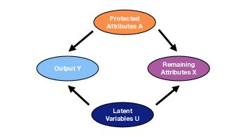
Figure 1: A causal model in a law school context. Directed edges between a source and a target denote a causal relationship in the sense that changing the value of the source (probabilistically) changes the value of the target. In this context, counterfactual fairness tries to make decisions based on knowledge (which cannot directly be measured) without biases from race or gender.

Counterfactual fairness offers a solution by advocating for a causal perspective, which provides statistical tools to help us minimize the direct effects of protected attributes on decisions (Kusner et al. 2017; Nilforoshan et al. 2022), and comports with a Rawlsian perspective of moral philosophy (Rawls 2004). It follows a surge of papers over the past decade that borrow intuition from moral philosophy to formally define what makes an algorithm fair (Dwork et al. 2012; Feldman et al. 2015; Hardt, Price, and Srebro 2016; Mitchell et al. 2021). Drawing from (Pearl et al. 2000)’s work on causal models, (Kusner et al. 2017) imagine a counterfactual world where only the protected attributes of observations are changed. Then, an algorithm is counterfactually fair if it makes the same predictions for a hypothetical counterfactual version of an observation as it would for the real version of the observation. This individual notion of fairness promises to avoid the pitfalls of the group based fairness measures we described earlier, though the relationship between causality, counterfactuals and moral philosophy is complicated (Kasirzadeh and Smart 2021).

Preliminaries and Notation

We follow notation laid out by (Kusner et al. 2017) for our formal analysis. The variables are partitioned into $A$ (the set of protected attributes), $U$ (the set of latent attributes), $X$ (the set of remaining variables), and $Y$ (the outcomes).

Figure 2 shows a general causal model. Each variable is generated (probabilistically) from a governing distribution. The parameters of a variable’s distribution are fixed or derived from the incoming edges in the causal model (or both). For example, we may have $a\sim\textrm{Binom}(.3,1)$, $u\sim\mathcal{N}(0,1)$, and $x\sim\textrm{Pois}(au)$.

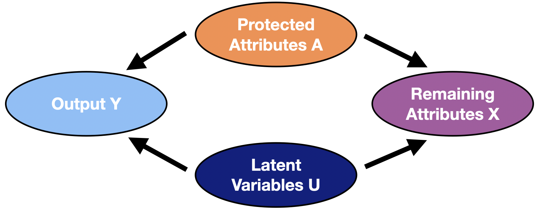
Figure 2: A general causal model consists of a directed acyclic graph and governing equations for the (probabilistic) generation of each variable.

A counterfactually fair algorithm uses $U$ to predict $Y$ since every other attribute is influenced by the protected attributes $A$. However, $U$ cannot be measured directly. The solution of counterfactual fairness is to model the joint distribution of each attribute in $X$ induced by the values of $A$ and $U$. Then $U$ is estimated by the posterior distribution on instances of $A$ and $X$.

Building a causal model requires domain expert knowledge to establish both the direction of relationships between attributes and the family of distributions (e.g., normal, Poisson, binomial, etc.) that generates the distribution of each variable. Once a causal model is determined, it is computationally intensive to learn the parameters of each distribution and then to estimate the posterior distribution of each attribute in $U$.

Fairness Definitions

In this section, we formalize the definitions of demographic parity and counterfactual fairness. We use capital letters $A$, $X$, $U$, and $Y$ to refer to sets of random variables, and we use lowercase letters $a$, $x$, $u$, and $y$ to refer to realizations of these random variables. Consider a predictor $\hat{Y}:A\times U\times X\rightarrow Y$. If a predictor $\hat{Y}$ does not use a particular set of random variables then we omit that set. We use $\hat{Y}_{A\leftarrow a}(u)$ for some protected group $a\in A$ to denote the prediction on $u$ where attributes in $A$ are set to $a$.

Definition 1 (Demographic Parity (Calders, Kamiran, and Pechenizkiy 2009; Zliobaite 2015; Zafar et al. 2015)).

Given a predictor $\hat{Y}:X\times A\rightarrow Y$, we say $\hat{Y}$ satisfies demographic parity if, for all instances of protected attributes $a$ and $a^{\prime}$,

$$\Pr(\hat{Y}(x,a)=y|A=a)=\Pr(\hat{Y}(x,a^{\prime})=y|A=a^{\prime})$$

where the probability is taken over the conditional distribution of $X$ and the possible randomness of $\hat{Y}$.

Definition 2 (Counterfactual Fairness (Kusner et al. 2017)).

Let $A$, $U$, $X$, and $Y$ be sets of random variables in a given causal model with specified distributions for each attribute. Consider any protected group $a^{\prime}\in A$ and any outcome $y\in Y$. Then a predictor $\hat{Y}:U\times A\rightarrow Y$ is counterfactually fair if for all observations $x\in X$ and $a\in A$,

$$\Pr(\hat{Y}_{A\leftarrow a}(u)=y|X=x,A=a)$$

$$=\Pr(\hat{Y}_{A\leftarrow a^{\prime}}(u)=y|X=x,A=a)$$

where the probability is with respect to the posterior distribution of $u$ induced by fixed observations $x$ and $a$.

Definition 2 states that it must be the case that the final prediction of a counterfactually fair predictor $\hat{Y}_{A\leftarrow a}(u)$ is distributed like $\hat{Y}_{A\leftarrow a^{\prime}}(u)$ when $a\neq a^{\prime}$ and where the distribution of $u$ is induced by observations of $X$ and $A$.

Now we have established the two primary definitions of fairness that we consider in our work. However, it is worth noting that difficulties in defining algorithmic fairness have led to many competing approaches. Furthermore, formal results have demonstrated the incompatibility of applying some fairness definitions in conjunction with others, which hints at irreconcilable philosophical groundings and a need for formalizations for different policy settings (Kleinberg, Mullainathan, and Raghavan 2016; Chouldechova 2016; Corbett-Davies and Goel 2018).

Our Contributions

Our work starts with a simple observation on the distribution of latent variables: by their definition, latent variables must be independent of protected attributes for the model to be counterfactually fair. A careful look at this statement suggests a connection to demographic parity, which requires that predictions must be independent of protected attributes. A natural question is then:

Do algorithms that satisfy demographic parity also satisfy counterfactual fairness?

But for an algorithm to even satisfy the definition of counterfactual fairness, we need a causal model, latent variables, and a way of estimating latent variables. Our first result answers the question in the affirmative if we trivially construct the necessary counterfactual fairness machinery.

The next natural question is whether the converse holds:

Do algorithms that satisfy counterfactual fairness also satisfy demographic parity?

We answer this question in the affirmative, as well. Together, the two results suggest that counterfactual fairness is basically demographic parity. This relationship is important for the fairness community since counterfactual fairness is often celebrated as a novel tool for fair decisions while demographic parity is considered simple and flawed. For example, in (Caton and Haas 2020), they note that demographic parity is flawed because it does not account for potential differences between groups, but do not mention limitations of counterfactual fairness. Other influential work takes a similar position (Gajane and Pechenizkiy 2017; Corbett-Davies and Goel 2018; Coston et al. 2020).

We also analyze three existing algorithms for counterfactual fairness in comparison to three benchmark algorithms. The data set is based on the running law school example and we corroborate our findings on two additional data sets and causal models. Our analysis uses a relaxation of counterfactual fairness and Kruskal-Wallis H tests (as one-sided tests for independence). We find that two simple benchmark algorithms outperform the existing algorithms in terms of satisfying the requirements of counterfactual fairness, computational efficiency, and accuracy.

We also introduce a notion of preserving group ordering. Put simply, it requires that an individual who performs better than another individual in the same protected group under unfair labels must also perform better than that individual under fair labels. We believe that this definition is important for transparency and consistency, laying the foundations for trust in fair algorithms. Why? Because inexplicable decisions in purportedly “fair” decision making processes can mask unforeseen technical bias (Abdollahi and Nasraoui 2018; Bhatt et al. 2020). Interestingly, we show that preserving group ordering can be mutually exclusive with counterfactual fairness for certain causal models. Empirically, we find the existing algorithms for counterfactual fairness have remarkably unstable orderings while the simple benchmark algorithms are consistent by design.

Outline

• We first show that all counterfactually fair predictors satisfy demographic parity and all predictors satisfying demographic parity can be trivially modified to satisfy counterfactual fairness.

• We subsequently analyze six algorithms (including those presented in (Kusner et al. 2017)) in the context of the following two questions:

  • How do these algorithms satisfy three special fairness constraints (counterfactual fairness, demographic parity, and the independence required for latent variables) while still maintaining reasonably accurate predictions?

  • How do these algorithms compare on the predictions they make at the individual level?

We corroborate our empirical results on additional data sets in the context of healthcare and loans. All our code and results are available online.

Related Work

Since its introduction, counterfactual fairness has been highly influential. Many recent works on equity in statistics and machine learning directly use or modify only slightly Definition 2 to enable training classifiers and other decision making algorithms (Zhang and Bareinboim 2018; Chiappa 2019; Wu, Zhang, and Wu 2019; Coston et al. 2020; Black, Yeom, and Fredrikson 2020; Mhasawade and Chunara 2021; Chikahara et al. 2021; von Kügelgen et al. 2022). (Zhang and Bareinboim 2018) create a procedure for identifying discrimination and applying causal explanations, and then use counterfactuals to design repairs while offering evaluations of this system on a host of examples. (Wu, Zhang, and Wu 2019) and (Chiappa 2019) expand theoretical groundings for counterfactual fairness, with the former improving on the latent attribute identifiability by offering bounds and techniques. Prior work also expands counterfactual fairness to deal with between-group rankings (Yang, Loftus, and Stoyanovich 2020). Furthermore, task specific variations and implementations of Definition 2 also exist for the medical domain (Pfohl et al. 2019), variational autoencoders in computer vision (Kim et al. 2021), generative-adversarial networks (Xu et al. 2019), and even natural language processing (Sarı, Hasegawa-Johnson, and Yoo 2021).

There are several existing concerns about counterfactual fairness. Recent work by (Nilforoshan et al. 2022) present a result that unites many causal notions of fairness, and further cautions that a gap exists between the effects of these popular approaches on fairness and their consequences, highlighting both practical and mathematical limitations. With particular relevance to our work, they show that when a predictor satisfying demographic parity and a causal model are specified, the predictor does not necessarily satisfy counterfactual fairness (see Theorem 2). In contrast, our work considers the setting where we are only given a predictor satisfying demographic parity (not a causal model) and can build a causal model of our choice. In (Kasirzadeh and Smart 2021), the authors conclude that counterfactual fairness may require what they deem to be an “incoherent theory” of social categories, i.e., some social categories may not admit counterfactual manipulation. In (Kilbertus et al. 2020), they examine the sensitivity of counterfactual fairness to “unmeasured confounding.” This is when a true causal effect between variables can be at least partially described by a non-zero correlation between two of the $\epsilon$-“error” variables calculated during one possible counterfactual fairness process, which can affect the independence guarantee from $A$. We position our work as an important addition to this existing set of papers expressing concerns with and limitations of counterfactual fairness.

Better understanding the theoretical and practical consistency of algorithmic fairness has real social impact. As fairness is operationalized through open source libraries like Fairlearn (Bird et al. 2020) and AIF360 (Bellamy et al. 2019), work that furthers our understanding of fair model guarantees becomes increasingly important.

Demographic Parity Is Counterfactual Fairness

Our results start with a simple observation about the definition of latent variables. In the original counterfactual fairness paper, the authors define latent variables $U$ so that “$U$ is a set of latent background variables, which are factors not caused by any variable in the set $V[=A\cup X]$ of observable variables” where $A$ is the set of protected attributes and $X$ is the set of remaining variables (Kusner et al. 2017). In other words, there are no incoming edges to $U$ in the causal model. This means that instances of latent variables are generated from a fixed set of parameters (that do not depend on protected attributes). In addition, while not explicitly stated in the definition, all causal models we are aware of also do not have any incoming edges to $A$. This means that instances of protected attributes are generated from a fixed set of parameters (that do not depend on latent variables). Together, these observations imply the following:

Criteria 3.

Latent variables are independent of protected attributes.

This criteria is key to understanding practical applications of counterfactual fairness. Counterfactual fairness attempts to explain behavior from protected attributes and latent variables. The protected attributes hold information on features outside of individuals’ control which would very often be unfair to base decisions on while the latent variables contain information on features within an individual’s control which are fair to base decisions on. From this perspective, it is clear that latent variables must be independent of protected attributes. Otherwise, this would imply that the inherent ‘worthiness’ of latent variables would problematically depend on protected attributes like race, gender, and age.

With Criteria 3 in hand, we show that any predictor which satisfies demographic parity also satisfies counterfactual fairness after a trivial modification.

Note that a predictor which satisfies counterfactual fairness must have an internal method of estimating latent variables and a causal model. So to say that a predictor which satisfies demographic parity also satisfies counterfactual fairness, we must introduce such a method and causal model. We do so in the proof of the first theorem in a trivial way.

Theorem 4.

Any predictor $\hat{Y}^{\prime}:X\times A\rightarrow Y$ that satisfies demographic parity can be modified into a method for estimating latent variables and a predictor $\hat{Y}:U\times A\rightarrow Y$ that is counterfactually fair.

Proof.

Our estimate of the latent variables $u$, given protected attributes $a$ and remaining attributes $x$, is $u=\hat{Y}^{\prime}(x,a)$. Then the predictor $\hat{Y}:U\times A\rightarrow Y$ is given by the identity function $\hat{Y}_{A\leftarrow a}(u)=u$. Because $\hat{Y}^{\prime}$ satisfies demographic parity, we know $\Pr(u|a)=\Pr(u|a^{\prime})$ for $a,a^{\prime}\in A$. That is, latent variables are independent of protected attributes which meets Criteria 3. Further, $\hat{Y}$ satisfies counterfactual fairness because $\hat{Y}_{A\leftarrow a}(u)=u=\hat{Y}_{A\leftarrow a^{\prime}}(u)$. ∎

The next theorem proves the converse of Theorem 4; namely, any counterfactually fair predictor also satisfies demographic parity.

Theorem 5.

Consider a method for estimating latent variables and a counterfactually fair predictor $\hat{Y}:U\times X\rightarrow Y$. Then the resulting predictor $\hat{Y^{\prime}}:X\times A\rightarrow Y$ satisfies demographic parity.

Proof.

Since the predictor is counterfactually fair, we know

$$\Pr(\hat{Y}_{A\leftarrow a}(u)=y|x,a)=\Pr(\hat{Y}_{A\leftarrow a^{\prime}}(u)=y|x,a)$$ (1)

for all $y\in Y$ where the realization of latent variables $u\in U$ is estimated from observations $a\in A$ and $x\in X$. Taking a weighted sum (if $X$ contains continuous random variables, an analogous statement holds via integration) of the right side of Equation (1) yields

$$\sum_{x\in X}\Pr(x|a)\Pr(\hat{Y}_{A\leftarrow a}(u)=y|x,a)$$

$$=\sum_{x\in X}\Pr(x,\hat{Y}_{A\leftarrow a}(u)=y|a)$$

$$=\Pr(\hat{Y}_{A\leftarrow a}(u)=y|a)=\Pr(\hat{Y}_{A\leftarrow a}(u)=y).$$

The first equality holds because $\Pr(x|a)\Pr(y|x,a)=\Pr(x,y|a)$ for random events $x,y,a$. The last equality holds by Criteria 3 and since the (possible) randomness of $\hat{Y}_{A\leftarrow a}(u)$ only comes from $u$ and the assignment $A\leftarrow a$. The final equality gets us close to demographic parity but the predictions could still depend on the assignment. We repeat the same steps for the left side of Equation (1) and find that

$$\Pr(\hat{Y}_{A\leftarrow a}(u)=y)=\Pr(\hat{Y}_{A\leftarrow a^{\prime}}(u)=y).$$

This tells us that the distribution of predictions made by a counterfactually fair algorithm are independent of protected attributes. That is, demographic parity holds. ∎

Note that the contrapositive of Theorem 5 gives us a simple way to test whether a predictor is counterfactually fair.

Algorithms for Counterfactual Fairness

In this section, we empirically analyze six algorithms in the context of counterfactual fairness on the running law school example. We compare them in terms of how well they achieve demographic parity (Definition 1), counterfactual fairness (Definition 2), and independence between protected attributes and latent variables (Criteria 3). We also compare the algorithms’ test accuracy and the resulting trade-offs between fairness and performance. Finally, we investigate how predictions on individuals differ between the algorithms.

The Algorithms

The first three algorithms—referred to as “Levels 1, 2 and 3”—come from the original counterfactual fairness paper (Kusner et al. 2017). The next two algorithms are simple heuristics for demographic parity while the final algorithm is a straightforward learner without fairness constraints.

For all the algorithms we analyze, we use a linear regression model, $\ell_{2}$-norm loss, and Adam optimizer for learning. We describe the algorithms next.

Level 1

Since evaluating the relationships between variables in a causal model is computationally expensive, the first level only uses the remaining variables that are independent of protected attributes to learn the outcomes. In practice, scenarios where remaining variables are not at least partially conditioned on protected attributes are so rare as to be virtually non-existent. Instead, we implement Level 1 by using all remaining variables (without any protected attributes). This approach has been called “fairness through unawareness” (Grgic-Hlaca et al. 2016) and fails to make fair decisions because protected attributes are often redundantly encoded (Pedreshi, Ruggieri, and Turini 2008).

Level 2

The second level uses the full power of causal models, but suffers from expensive and intensive computations; it requires domain expertise to specify the joint distributions over all variables for the causal model. Remaining variables are distributed according to subsets of latent variables and protected attributes. By using the known protected attributes, the remaining variables, and the causal model, Level 2 estimates likely values of latent variables. Then only the latent variables are used to learn a predictor over the set of possible outcomes.

Level 3

The third level is a compromise between the simplicity of Level 1 and complexity of Level 2. Level 3 uses the relationships in the causal model to express the remaining variables of each individual as a deterministic function of related protected attributes and a special explanation term. The deterministic function is learned from protected attributes to explain the remaining variable. Then the difference between the deterministic function and an individual’s remaining variable is their explanation term. These explanation terms are used to learn the outcomes.

Listing 1: Converting unfair predictions to fair predictions when labels are normally distributed.

⬇

1Input: $n$ group identities $a_{i}\in A$ and unfair labels $\bar{y_{i}}$ for samples $i\in[n]$

2Output: predictions $\hat{y}_{i}$ that satisfy demographic parity

3$\mu\leftarrow$ mean($\{\bar{y}_{i}:i\in[n]\}$)

4$\sigma\leftarrow$ std($\{\bar{y}_{i}:i\in[n]\}$)

5for $a$ in $A$ do

6 $\mu_{a}\leftarrow$ mean($\{\bar{y}_{i}:a_{i}=a\}$)

7 $\sigma_{a}\leftarrow$ std($\{\bar{y}_{i}:a_{i}=a\}$)

8 for $i$ in $\{i:a_{i}=a\}$ do

9 $\hat{y_{i}}=\mu+\sigma(\bar{y}_{i}-\mu_{a})/\sigma_{a}$

Listing 2: Converting unfair predictions to fair predictions under any distribution of labels.

⬇

1Input: $n$ group identities $a_{i}\in A$ and unfair labels $\bar{y_{i}}$ for samples $i\in[n]$

2Output: predictions $\hat{y}_{i}$ that satisfy demographic parity

3$CDF\leftarrow$ empirical CDF of $\{y_{i}:i\in[n]\}$

4for $a$ in $A$ do

5 $CDF_{a}\leftarrow$ empirical CDF of $\{y_{i}:a_{i}=a\}$

6 for $i$ in $\{i:a_{i}=a\}$

7 $\hat{y}_{i}\leftarrow CDF(CDF_{a}^{-1}(\bar{y}_{i}))$

The next two algorithms are simple heuristics for demographic parity.

Listing 1

The first listing assumes the distribution of outcomes in every protected group is normally distributed. Then we can achieve demographic parity by simply calculating the normalized score of each individual within their protected group and converting it to the outcome distribution of the full population.

Listing 2

The second listing drops the assumption on the distribution of each protected group. Instead, Listing 2 estimates the cumulative density function (CDF) of each protected group and converts an individual’s relative position within their group to the same position within the full population.

Listing 1 is appropriate when the outcomes are normally distributed while Listing 2 is appropriate in general but cannot distinguish noise from signal in distributions.

Full Linear Model

The final algorithm uses a linear model on all protected attributes and remaining variables to learn outcomes. We expect the full linear model to mimic the unfair behavior of the underlying data but achieve the best test accuracy.

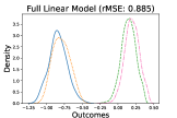
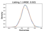
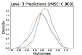
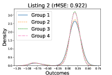
Figure 3: Density plots for the distributions over predictions made by the six algorithms we consider. The root mean squared error (rMSE) is given next to each title and in Table 2. Groups 1, 2, 3, and 4 correspond to protected groups over the Cartesian product of binary race and gender.

Measures of Fairness

We use several empirical tests to measure how well each of the algorithms achieves different definitions of fairness.

We first define a relaxation of counterfactual fairness introduced in (Russell et al. 2017).

Definition 6 ($(\epsilon,\delta)$-Approximate Counterfactual Fairness (ACF)).

A predictor $\hat{Y}:X\times A\rightarrow Y$ satisfies $(\epsilon,\delta)$-ACF if

$$\Pr(|\hat{Y}_{A\leftarrow a}(u)-\hat{Y}_{A\leftarrow a^{\prime}}(u)|\leq\epsilon|x,a)\geq 1-\delta.$$

Notice that calculating $(\epsilon,\delta)$-ACF requires an internal estimate of latent variables. The only algorithms that have a nontrivial estimate of latent variables are Level 2 and Level 3. Since both Level 2 and Level 3 use only the latent variables in learning the outcomes, changing the protected attribute has no effect and both algorithms are $(0,0)$-ACF.

For testing demographic parity and whether latent variables are independent of protected attributes, we use the Kruskal-Wallis H test (Kruskal and Wallis 1952).

Definition 7 (Kruskal-Wallis H Statistic).

The H statistic is given by

$$(N-1)\frac{\sum_{i=1}^{g}n_{i}(\bar{r}_{i}-\bar{r})^{2}}{\sum_{i=1}^{g}\sum_{j=1}^{n_{i}}(r_{ij}-\bar{r})^{2}}$$

where $N$ is the total number of observations, $g$ is the number of groups, $n_{i}$ is the number of observations in group $i$, $r_{ij}$ is the rank (among all observations) of observation $j$ from group $i$, $\bar{r}_{i}$ is the average rank of observations in group $i$, and $\bar{r}$ is the average rank of all observations.

Using the Kruskal-Wallis H statistic, we can calculate the probability that every group comes from a distribution with the same median. Since the latent variables are independent of the protected attributes if and only if the distributions of the protected groups are the same, a small probability from the Kruskal-Wallis H test implies that the latent variables and protected attributes are not independent. We also use the test to determine whether an algorithm satisfies demographic parity. Note it is possible that all groups come from distributions with the same median but that the distributions are in fact different so the test has one-sided error.

We present our results of the Kruskal-Wallis H tests in Table 1. The first three data rows tell us the probability that Criteria 3 holds. It is very likely that the latent variables in each protected group come from distributions with the same median in Level 2, suggesting that Level 2 satisfies Criteria 3 in addition to counterfactual fairness. In contrast, it is unlikely (probability $<.05$) that the two latent variables in Level 3 are independent of protected attributes, suggesting that Level 3 does not satisfy Criteria 3. Note that Level 3 is an example of an algorithm that ostensibly satisfies counterfactual fairness but the latent variables do not meet the necessary condition of Criteria 3. We corroborate this finding in Figure 3: Level 1 and Level 3 clearly do not satisfy demographic parity because the latent variables are not independent of protected attributes.

The last six rows in Table 1 tell us whether each algorithm satisfies demographic parity. As expected, Level 1 and the Full Linear Model are remarkably unlikely to satisfy demographic parity. In line with the results for latent variables, we see that Level 3 also is unlikely to satisfy demographic parity. Finally, Level 2 likely satisfies demographic parity. This is to be expected since the assumptions of Theorem 5—namely, counterfactual fairness and Criteria 3—hold. Of course, Listings 1 and 2 are very likely to satisfy demographic parity by design.

Variable	H Statistic	$p$-value
Level 2 Latent Variable	$.347$	$.951$
Level 3 Latent UGPA	$10.8$	$.0126$
Level 3 Latent LSAT	$84.6$	$3.21\times 10^{-18}$
Level 1 Predictions	$221$	$9.81\times 10^{-48}$
Level 2 Predictions	$.346$	$.951$
Level 3 Predictions	$69.3$	$5.97\times 10^{-15}$
Listing 1 Predictions	$.165$	$.983$
Listing 2 Predictions	$.035$	$.998$
Full Predictions	$829$	$2.53\times 10^{-179}$

Table 1: Kruskal-Wallis H test results for different variables. The $p$-value indicates the likelihood of observing the H statistic if the variable was distributed the same in every group. Every number is reported to three significant figures.

Table 2 gives the root mean squared error (rMSE) of every algorithm we consider. As expected, the Full Linear Model without fairness constraints has the lowest error. Listing 1 and Listing 2 also give relatively low error. In contrast, Level 2 has the highest error. So far, Level 2 simulatenously satisfies Definition 1, Definition 2, and Criteria 3 but we see this is at the expense of accuracy.

Lvl 1	Lvl 2	Lvl 3	Lst 1	Lst 2	Full
.933	.936	.908	.919	.921	.881

Table 2: The root mean squared error (rMSE) for each algorithm predicted to three significant figures.

Individual Predictions

We have seen how the algorithms we consider perform differently in terms of three fairness measures. But how do the algorithms differ on the actual outcomes for individuals?

Figure 4 visualizes the change in relative ordering of predicted outcomes for 40 randomly chosen individuals in Group 1 (Black men) in the law school example. Notably, the relative ordering is constant between Listing 1, Listing 2, and the Full Linear Model, as expected. However, the relative ordering is highly unstable for Level 1, Level 2, and Level 3. This suggests that while Level 2 and Level 3 achieve counterfactual fairness, they do so in dramatically different ways. One explanation is that Level 2 satisfies Criteria 3 while Level 3 does not.

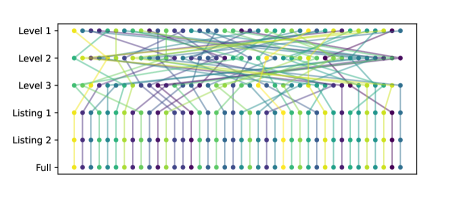
Figure 4: We randomly sample 40 individuals from Group 1 (Black men) in the law school example and visualize how the relative order of their predicted outcomes changes based on the algorithm making predictions.

We find it surprising that Level 2 does not agree with Listing 1 and Listing 2 on the relative order of outcomes. All three algorithms satisfy demographic parity, Criteria 3, and, by Theorem 4, counterfactual fairness (when Listing 1 and Listing 2 are trivially modified). How could it be that two algorithms are both fair under the same definitions while making radically different predictions on individuals?

This question suggests the following natural definition.

Definition 8 (Preserving Group Ordering).

Given unfair labels, we say an algorithm preserves group ordering if the relative ordering within each protected group under the unfair labels is the the same as the relative ordering of individuals induced by the algorithm’s predictions.

Put differently, if individuals are in the same protected class, then their relative ordering from a (possibly) unfair predictor should induce the same relative ordering as the fair predictor. That is, if an individual performs better under the same unfair conditions as another individual, they should perform better in a hypothetical world where those unfair conditions were removed.

We believe that preserved within-group orderings are preferable to the highly unstable orderings in the levels of (Kusner et al. 2017). One reason to prefer preserved orderings is that even soft guarantees for relative orderings of within group individuals leads to more transparent, trustworthy and ultimately useful fair algorithms (Abdollahi and Nasraoui 2018; Bhatt et al. 2020).

Observe that Listing 1 and Listing 2 satisfy Definition 8 by design. This contrasts with Levels 1, 2, and 3 which radically change the relative ordering of individuals within a protected group. In Proposition 9, we show that there is a causal model where counterfactual fairness is mutually exclusive with Definition 8. This suggests that for some causal models, achieving counterfactual fairness and preserving relative group ordering are incompatible.

Note that Proposition 9, combined with the fact that Listing 1 and 2 satisfy demographic parity and preserve group order, does not refute Theorem 4 since the method of estimating latent variables in the proof of the theorem uses a trivial causal model.

Proposition 9.

There is a causal model and predictor where a counterfactually fair algorithm does not maintain the relative ordering of predictions within each group.

	Short				Tall
	World A		World B		World A		World B
	$u$	$\hat{y}$	$u$	$\hat{y}$	$u$	$\hat{y}$	$u$	$\hat{y}$
Teal	0	0	1	1	0	1	1	0
Lucas	1	1	0	0	1	0	0	1

Table 3: Latent variable charm $U$ and predicted outcome $\hat{Y}$ for each person, world, and protected group in the example for Proposition 9.

Proof.

Consider an example with two people, say Teal and Lucas. The protected attribute $A$ is binary height, the latent variable $U$ is binary charm, and the true outcome $Y$ is binary success. The latent variable for Teal is $u_{\textrm{Teal}}\sim\textrm{Binomial}(1/2)$ while the latent variable for Lucas is $u_{\textrm{Lucas}}=1-u_{\textrm{Teal}}$. In other words, the latent variable for each person is probabilistic but correlated: with probability 1/2, we live in World A and otherwise, we live in World B. In World A, Teal is not charming and Lucas is while, in World B, Teal is charming and Lucas is not. Now the predictor function satisfies $\hat{Y}_{A\leftarrow\textrm{short}}(u)=u$, $\hat{Y}_{A\leftarrow\textrm{tall}}(u)=\texttt{NOT}(u)$ for latent variable charm $u\in\{0,1\}$. The output of the predictor in each world is given in Table 3.

Notice that the relative order of the outcome produced by the predictor and causal model changes with the counterfactual intervention. In World A, Teal is behind Lucas as a short person and ahead as a tall person. In World B, Teal is ahead of Lucas as a short person and behind as a tall person. We have constructed a causal model and predictor but it remains to show that they satisfy counterfactual fairness and that the latent variable is independent of protected attributes.

First, we show that the causal model and predictor are counterfactually fair. Recall that World A and World B are equally likely. As a result, by inspecting Table 3 and the construction, we conclude that both Teal and Lucas are as likely to be successful as a short person and as a tall person. Therefore the construction satisfies counterfactual fairness.

Second, we show that the latent variable is independent of the protected attribute. That is, we want to show $\Pr(u,a)=\Pr(u)\Pr(a)$ for $u,a\in\{0,1\}$ in our example. Again, by inspecting Table 3 and the construction, we see that this holds. For example, the probability a person is charming and tall is 2/8 while the probability a person is charming is 4/8 and the probability a person is tall is 4/8. The same holds for the other three possibilities. ∎

Additional Experiments

So far we have reported on the extensive empirical experiments we ran on the law school data set. We corroborate our findings by running the same set of experiments on two more examples. The first example is data from the Home Credit Default Risk data set. We simulated a “domain expert” process of causal analysis and constructed a credit risk causal model by hand (using observations from the data). The second example is synthetic data generated directly from a causal model we built, modeling a hypothetical healthcare context loosely motivated by (Obermeyer et al. 2019), and represents the “ideal” circumstance where the causal model posited over the data is certainly correct. We show the causal models in Figure 5. The remaining figures and results are included for reproducibility in the the same repository as the rest of our results.

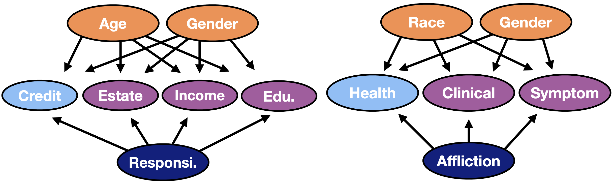
Figure 5: The causal diagrams for the default risk example (on the left) and healthcare example (on the right).

Conclusion

Counterfactual fairness has been celebrated as novel and promising while demographic parity has been treated as simple and flawed. Our work shows how the two definitions of fairness are basically equivalent when considered across an entire population. We think it is a promising avenue for future work to identify similarities between other definitions of fairness. We also introduce a method for comparing algorithms at the level of individual predictions. Our findings suggest a natural definition of preserving group orderings which can be mutually exclusive with counterfactual fairness. We leave open the problem of designing novel algorithms that are competitive with simple benchmarks in terms of fairness, performance, and preserving group orderings.

References

- Abdollahi and Nasraoui (2018) Abdollahi, B.; and Nasraoui, O. 2018. Transparency in fair machine learning: the case of explainable recommender systems. In Human and machine learning, 21–35. Springer.
- Bellamy et al. (2019) Bellamy, R. K.; Dey, K.; Hind, M.; Hoffman, S. C.; Houde, S.; Kannan, K.; Lohia, P.; Martino, J.; Mehta, S.; Mojsilović, A.; et al. 2019. AI Fairness 360: An extensible toolkit for detecting and mitigating algorithmic bias. IBM Journal of Research and Development, 63(4/5): 4–1.
- Bhatt et al. (2020) Bhatt, U.; Xiang, A.; Sharma, S.; Weller, A.; Taly, A.; Jia, Y.; Ghosh, J.; Puri, R.; Moura, J. M.; and Eckersley, P. 2020. Explainable machine learning in deployment. In Proceedings of the 2020 conference on fairness, accountability, and transparency, 648–657.
- Bird et al. (2020) Bird, S.; Dudík, M.; Edgar, R.; Horn, B.; Lutz, R.; Milan, V.; Sameki, M.; Wallach, H.; and Walker, K. 2020. Fairlearn: A toolkit for assessing and improving fairness in AI. Microsoft, Tech. Rep. MSR-TR-2020-32.
- Black, Yeom, and Fredrikson (2020) Black, E.; Yeom, S.; and Fredrikson, M. 2020. FlipTest: fairness testing via optimal transport. Proceedings of the 2020 Conference on Fairness, Accountability, and Transparency.
- Calders, Kamiran, and Pechenizkiy (2009) Calders, T.; Kamiran, F.; and Pechenizkiy, M. 2009. Building classifiers with independency constraints. In 2009 IEEE International Conference on Data Mining Workshops, 13–18. IEEE.
- Caton and Haas (2020) Caton, S.; and Haas, C. 2020. Fairness in machine learning: A survey. arXiv preprint arXiv:2010.04053.
- Chiappa (2019) Chiappa, S. 2019. Path-Specific Counterfactual Fairness. In AAAI.
- Chikahara et al. (2021) Chikahara, Y.; Sakaue, S.; Fujino, A.; and Kashima, H. 2021. Learning Individually Fair Classifier with Path-Specific Causal-Effect Constraint. In AISTATS.
- Chouldechova (2016) Chouldechova, A. 2016. Fair prediction with disparate impact: A study of bias in recidivism prediction instruments. arXiv:1610.07524.
- Corbett-Davies and Goel (2018) Corbett-Davies, S.; and Goel, S. 2018. The measure and mismeasure of fairness: A critical review of fair machine learning. arXiv preprint arXiv:1808.00023.
- Coston et al. (2020) Coston, A.; Mishler, A.; Kennedy, E. H.; and Chouldechova, A. 2020. Counterfactual risk assessments, evaluation, and fairness. In Proceedings of the 2020 conference on fairness, accountability, and transparency, 582–593.
- Dwork et al. (2012) Dwork, C.; Hardt, M.; Pitassi, T.; Reingold, O.; and Zemel, R. 2012. Fairness through awareness. In Proceedings of the 3rd innovations in theoretical computer science conference, 214–226.
- Fawkes, Evans, and Sejdinovic (2022) Fawkes, J.; Evans, R.; and Sejdinovic, D. 2022. Selection, Ignorability and Challenges With Causal Fairness. In First Conference on Causal Learning and Reasoning.
- Feldman et al. (2015) Feldman, M.; Friedler, S. A.; Moeller, J.; Scheidegger, C.; and Venkatasubramanian, S. 2015. Certifying and removing disparate impact. In proceedings of the 21th ACM SIGKDD international conference on knowledge discovery and data mining, 259–268.
- Gajane and Pechenizkiy (2017) Gajane, P.; and Pechenizkiy, M. 2017. On formalizing fairness in prediction with machine learning. arXiv preprint arXiv:1710.03184.
- Grgic-Hlaca et al. (2016) Grgic-Hlaca, N.; Zafar, M. B.; Gummadi, K. P.; and Weller, A. 2016. The case for process fairness in learning: Feature selection for fair decision making. In NIPS symposium on machine learning and the law, volume 1, 2.
- Hardt, Price, and Srebro (2016) Hardt, M.; Price, E.; and Srebro, N. 2016. Equality of opportunity in supervised learning. Advances in neural information processing systems, 29: 3315–3323.
- Kasirzadeh and Smart (2021) Kasirzadeh, A.; and Smart, A. 2021. The use and misuse of counterfactuals in ethical machine learning. In Proceedings of the 2021 ACM Conference on Fairness, Accountability, and Transparency, 228–236.
- Kilbertus et al. (2020) Kilbertus, N.; Ball, P. J.; Kusner, M. J.; Weller, A.; and Silva, R. 2020. The sensitivity of counterfactual fairness to unmeasured confounding. In Uncertainty in artificial intelligence, 616–626. PMLR.
- Kim et al. (2021) Kim, H.; Shin, S.; Jang, J.; Song, K.; Joo, W.; Kang, W.; and Moon, I.-C. 2021. Counterfactual Fairness with Disentangled Causal Effect Variational Autoencoder. In AAAI.
- Kleinberg, Mullainathan, and Raghavan (2016) Kleinberg, J.; Mullainathan, S.; and Raghavan, M. 2016. Inherent Trade-Offs in the Fair Determination of Risk Scores. arXiv:1609.05807.
- Kruskal and Wallis (1952) Kruskal, W. H.; and Wallis, W. A. 1952. Use of ranks in one-criterion variance analysis. Journal of the American statistical Association, 47(260): 583–621.
- Kusner et al. (2017) Kusner, M. J.; Loftus, J. R.; Russell, C.; and Silva, R. 2017. Counterfactual fairness. arXiv preprint arXiv:1703.06856.
- Mhasawade and Chunara (2021) Mhasawade, V.; and Chunara, R. 2021. Causal multi-level fairness. In Proceedings of the 2021 AAAI/ACM Conference on AI, Ethics, and Society, 784–794.
- Mitchell et al. (2021) Mitchell, S.; Potash, E.; Barocas, S.; D’Amour, A.; and Lum, K. 2021. Algorithmic fairness: Choices, assumptions, and definitions. Annual Review of Statistics and Its Application, 8: 141–163.
- Nilforoshan et al. (2022) Nilforoshan, H.; Gaebler, J. D.; Shroff, R.; and Goel, S. 2022. Causal Conceptions of Fairness and their Consequences. In ICML.
- Obermeyer et al. (2019) Obermeyer, Z.; Powers, B.; Vogeli, C.; and Mullainathan, S. 2019. Dissecting racial bias in an algorithm used to manage the health of populations. Science, 366(6464): 447–453.
- Pearl et al. (2000) Pearl, J.; et al. 2000. Models, reasoning and inference. Cambridge, UK: CambridgeUniversityPress, 19: 2.
- Pedreshi, Ruggieri, and Turini (2008) Pedreshi, D.; Ruggieri, S.; and Turini, F. 2008. Discrimination-aware data mining. In Proceedings of the 14th ACM SIGKDD international conference on Knowledge discovery and data mining, 560–568.
- Pfohl et al. (2019) Pfohl, S. R.; Duan, T.; Ding, D. Y.; and Shah, N. H. 2019. Counterfactual Reasoning for Fair Clinical Risk Prediction. ArXiv, abs/1907.06260.
- Rawls (2004) Rawls, J. 2004. A theory of justice. In Ethics, 229–234. Routledge.
- Russell et al. (2017) Russell, C.; Kusner, M. J.; Loftus, J.; and Silva, R. 2017. When worlds collide: integrating different counterfactual assumptions in fairness. Advances in neural information processing systems, 30.
- Sarı, Hasegawa-Johnson, and Yoo (2021) Sarı, L.; Hasegawa-Johnson, M.; and Yoo, C. D. 2021. Counterfactually fair automatic speech recognition. IEEE/ACM Transactions on Audio, Speech, and Language Processing, 29: 3515–3525.
- von Kügelgen et al. (2022) von Kügelgen, J.; Bhatt, U.; Karimi, A.-H.; Valera, I.; Weller, A.; and Scholkopf, B. 2022. On the Fairness of Causal Algorithmic Recourse. In AAAI.
- Wu, Zhang, and Wu (2019) Wu, Y.; Zhang, L.; and Wu, X. 2019. Counterfactual Fairness: Unidentification, Bound and Algorithm. In IJCAI.
- Xu et al. (2019) Xu, D.; Wu, Y.; Yuan, S.; Zhang, L.; and Wu, X. 2019. Achieving Causal Fairness through Generative Adversarial Networks. In IJCAI.
- Yang, Loftus, and Stoyanovich (2020) Yang, K.; Loftus, J. R.; and Stoyanovich, J. 2020. Causal intersectionality for fair ranking. arXiv preprint arXiv:2006.08688.
- Zafar et al. (2015) Zafar, M. B.; Valera, I.; Rodriguez, M. G.; and Gummadi, K. P. 2015. Learning fair classifiers. arXiv preprint arXiv:1507.05259, 1(2).
- Zhang and Bareinboim (2018) Zhang, J.; and Bareinboim, E. 2018. Fairness in Decision-Making - The Causal Explanation Formula. In AAAI.
- Zliobaite (2015) Zliobaite, I. 2015. On the relation between accuracy and fairness in binary classification. arXiv preprint arXiv:1505.05723.