Field-Induced Boson Insulating States in a 2D Superconducting Electron Gas with Strong Spin-Orbit Scatterings

Abstract

The phenomenon of field-induced superconductor-to-insulator transitions observed experimentally in electron-doped SrTiO₃/LaAlO₃ interfaces, analyzed recently by menas of 2D superconducting fluctuations theory (Phys. Rev. B 104, 054503 (2021)), is revisited with new insights associating it with the appearnace at low temperatures of field-induced boson insulating states. Within the framework of the time-dependent Ginzburg-Landau approach, we pinpoint the origin of these states in field-induced extreme softening of fluctuation modes over a large region in momentum space, upon diminishing temperature, which drives Cooper-pair fluctuations to condense into mesoscopic puddles in real space. Dynamical quantum tunneling of Cooper-pair fluctuations out of these puddles, introduced within a phenomenological approach, which break into mobile single-electron states, contains the high-field resistance onset predicted by the exclusive boson theory.

I
Introduction

In a recent paper MZPRB2021 we have shown that Cooper-pair fluctuations in a 2D electron gas with strong spin-orbit scatterings can lead at low temperatures to pronounced magnetoresistance (MR) peaks above a crossover field to superconductivity. The model was applied to the high mobility electron systems formed in the electron-doped interfaces between two insulating perovskite oxides—SrTiO₃ and LaAlO₃ Ohtomo04 ,Caviglia08 , showing good quantitative agreement with a large body of experimental sheet-resistance data obtained under varying gate voltage Mograbi19 .

The model employed was based on the opposing effects generated by fluctuations in the superconducting (SC) order parameter: The nearly singular enhancement of conductivity (paraconductivity) due to fluctuating Cooper pairs below the nominal (mean-field) critical magnetic field, on one hand, and the suppression of conductivity, associated with the loss of unpaired electrons due to Cooper pairs formation, on the other hand. The self-consistent treatment of the interaction between fluctuations UllDor90 ,UllDor91 , employed in these calculations, avoids the critical divergence of both the Aslamazov-Larkin (AL) paraconductivity AL68 and the DOS conductivity LV05 , allowing to extend the theory to regions well below the nominal critical SC transition. The absence of long range phase coherence implied by this approach is consistent with the lack of the ultimate zero-resistance state in the entire data analyzed there.

The most intriguing question arising from the Cooper-pair fluctuations scenario of the superconductor–insulator transition (SIT) presented in Ref.MZPRB2021 , is how Cooper-pairs liquid, whose condensation (in momentum space) is customarily associated with superconductivity, could metamorphose into an insulator just by lowering its temperature under sufficiently high magnetic field ?

For answering this intriguing question we note our use of the time-dependent Ginzburg-Landau (TDGL) functional approach in consistently evaluating the AL and the DOS conductivities. Within this exclusive boson approach we have found in Ref.MZPRB2021 that at low temperatures the (negative) DOS conductivity prevails over the AL paraconductivity at fields that roughly indicate the presence of the observed enhanced MR. Dynamical quantum tunneling of Cooper-pair fluctuations out of mesoscopic puddles has been introduced into the theory within a complementary phenomenological approach, including the contribution of unpaired normal electron states, to account for the observed experimental data.

In the present paper we reveal the underlying origin of these low-temperature field-induced boson insulating states by exploiting a detailed analytical scheme within the framework of the TDGL functional approach. It is found that strong field-induced suppression of the fluctuation stiffness parameter at low temperatures resulting in extreme softening of fluctuating modes over a large region in momentum space, dramatically enhances the Cooper-pair fluctuations density in mesoscopic puddles of real space. The resulting large enhancement of the (negative) DOS conductivity versus the diminishing AL paraconductivity, associated with the fluctuation mass enhancement, trigger the appearance of insulating states at high field. Our detailed analysis has also illuminated the mechanism in which the exclusive fluctuation boson picture is modified within a unified phenomenological approach. It allows field-induced pair-breaking processes to develop during dynamical quantum tunneling of Cooper-pair fluctuations out of mesoscopic puddles, which result in free exchange between the systems of charge-bosons and unpaired free electrons.

II The TDGL functional approach

The TDGL functional $\mathfrak{L}\left(\Delta,\mathbf{A}\right)$ of the order parameter $\Delta\left(\boldsymbol{r},t\right)$ and vector potential $\mathbf{A}\left(\boldsymbol{r},t\right)$ determines the Cooper-pairs current density FuldeMaki70 :

$$\mathbf{j}\left(\mathbf{r},t\right)=\frac{\partial\mathfrak{L}\left(\Delta\left(\mathbf{r},t\right),\mathbf{A}\left(\mathbf{r},t\right)\right)}{\partial\mathbf{A}\left(\mathbf{r},t\right)}$$ (1)

responsible for the AL paraconductivity. In this approach the entire underlying information about the thin film of pairing electrons system (which includes in-plane spin-orbit scatterings, Zeeman spin splitting as well as out-of-plane diamagnetic energy MZPRB2021 ) is incorporated in the inverse fluctuation propagator (in wavevector-frequency representation) $D^{-1}\left(\mathbf{q+}2e\mathbf{A/\hbar},\omega\right)$, mediating between the order parameter and the GL functional. In the Gaussian approximation the relation is quadratic, i.e.:

$$\mathfrak{L}\left(\Delta,\mathbf{A}\right) = \left(\frac{1}{2\pi}\right)^{2}d^{-1}\int d^{2}q\left(\frac{1}{2\pi}\right)$$

$$\times\int d\Omega\left|\Delta\left(\mathbf{q},\Omega\right)\right|^{2}D^{-1}\left(\mathbf{q+}2e\mathbf{A/\hbar},\Omega\right)$$

so that the coupling to the external electromagnetic field takes place directly through the vertex of the Cooper-pair current, defined in Eq.(1).

The corresponding AL time-ordered current-current correlator is given by:

$$Q_{AL}\left(i\Omega_{\nu}\right)=\left(4eN_{2D}D\right)^{2}d^{-1}\left(\frac{1}{2\pi}\right)^{2}\int d^{2}qq_{x}^{2}k_{B}T$$ (3)

$$\sum\limits_{\mu=-\infty}^{\infty}C\left(q,\Omega_{\mu}+\Omega_{\nu}\right)D\left(q,\Omega_{\mu}+\Omega_{\nu}\right)C\left(q,\Omega_{\mu}\right)D\left(q,\Omega_{\mu}\right)$$

where $\Omega_{\mu}=2\mu k_{B}T/\hbar,\Omega_{\nu}=2\nu k_{B}T/\hbar,$ $\mu=0,\pm 1,\pm 2,...,$    $\nu=0,1,2,....$ are bosonic Matsubara frequencies, $d$ is the thickness of the detected film, and $N_{2D}=m^{\ast}/2\pi\hbar^{2}$ is the single-electron DOS, with an effective mass $m^{\ast}$. Here the electrical current is generated along the $x$ axis, $q_{z},q_{x}$ are the fluctuation (in-plane) wave-vector components along the magnetic and electric field directions, respectively, and $q^{2}\equiv q_{z}^{2}+q_{x}^{2}$.

Explicitly for the model of spin-orbit scatterings employed, the fluctuation propagator $D\left(q,\Omega_{\mu}\right)$ and its corresponding effective current vertex $C\left(q,\Omega_{\mu}\right)$ are given by MZPRB2021 :

$$D\left(q,\Omega_{\mu}\right) = \frac{1}{N_{2D}\Phi\left(x+\left|\mu\right|;\varepsilon_{H}\right)},$$

$$C\left(q,\Omega_{\mu}\right) = \frac{1}{4\pi k_{B}T}\Phi^{\prime}\left(x+\left|\mu\right|;\varepsilon_{H}\right)$$ (4)

where

$$\Phi\left(x+\left|\mu\right|;\varepsilon_{H}\right)=\varepsilon_{H}+$$

$$\begin{array}[]{c}a_{+}\left[\psi\left(1/2+f_{-}+x+\left|\mu\right|\right)-\psi\left(1/2+f_{-}\right)\right]\\ +a_{-}\psi\left[\left(1/2+f_{+}+x+\left|\mu\right|\right)-\psi\left(1/2+f_{+}\right)\right]\end{array}$$ (7)

and:

$$\varepsilon_{H}\equiv\ln\left(\frac{T}{T_{c0}}\right)+a_{+}\psi\left(\frac{1}{2}+f_{-}\right)+a_{-}\psi\left(\frac{1}{2}+f_{+}\right)-\psi\left(1/2\right)$$ (8)

Here $T_{c0}$ is the mean-field SC transition temperature at zero magnetic field, $\psi$ is the digamma function, $x=\hbar Dq^{2}/4\pi k_{B}T$, where $D\equiv\tau_{SO}E_{F}/m^{\ast}$ is the electron diffusion coefficient, $E_{F}$- the Fermi energy, and $\varepsilon_{SO}=\hbar/\tau_{SO}$ is the spin-orbit energy. The system parameters: $\ f_{\pm}=\delta H^{2}+\beta\pm\sqrt{\beta^{2}-\mu^{2}H^{2}}$, $a_{\pm}=\left(1\pm\beta/\sqrt{\beta^{2}-\mu^{2}H^{2}}\right)/2$ are dimensionless functions of the magnetic field $H$, with the basic parameters: $\ \beta\equiv\varepsilon_{SO}/4\pi k_{B}T,$ $\delta\equiv D\left(de\right)^{2}/2\pi k_{B}T\hslash$, $\mu\equiv\mu_{B}/2\pi k_{B}T\$and $\mu_{B}$ the Bohr magneton.

The DOS conductivity is obtained within this TDGL functional approach by exploiting the Drude formula $\sigma_{DOS}=-2n_{s}e^{2}\tau_{SO}/m^{\ast}$, through the Cooper-pair fluctuations density $n_{s}$ LV05 :

$$n_{s}=\frac{1}{d}\frac{1}{\left(2\pi\right)^{2}}\int\left\langle\left|\phi\left(q\right)\right|^{2}\right\rangle d^{2}q$$ (9)

with the Cooper-pair momentum distribution function $\left\langle\left|\phi\left(q\right)\right|^{2}\right\rangle$ derived by exploiting the frequency-dependent GL functional, Eq.(II). This is done by rewriting Eq.(II) in terms of the frequency and wavenumber representations GL wave functions $\phi\left(q,\Omega\right)$, after analytic continuation to real frequencies $i\Omega_{\mu}\rightarrow\Omega$, i.e.:

$$\mathfrak{L}\left(\Delta\right) = \int\frac{d^{2}q}{\left(2\pi\right)^{2}}\int\frac{d\Omega}{2\pi}\left|\Delta\left(q,\Omega\right)\right|^{2}D\left(q,\Omega\right)^{-1}$$

$$= \int\frac{d^{2}q}{\left(2\pi\right)^{2}}\int\frac{d\Omega}{2\pi}\left|\phi\left(q,\Omega\right)\right|^{2}L\left(q,\Omega\right)^{-1}=\mathfrak{L}\left(\phi\right)$$

where the transformed inverse propagator $L\left(q,\Omega\right)^{-1}$ given by:

$$N_{2D}D\left(q,\Omega\right)=\mathcal{A}k_{B}TL\left(q,\Omega\right)$$

and: $\mathcal{A}\equiv 4\pi^{2}k_{B}T/7\zeta\left(3\right)E_{F}$, with: $\zeta\left(3\right)\simeq 1.202$.

For the sake of clarity of the analysis that follows we expand $L^{-1}\left(q,\Omega\right)$ to leading orders in small $q$ and $\Omega$, i.e.:

$$L^{-1}\left(q,\Omega\right)\simeq\mathcal{A}k_{B}T\left[\varepsilon_{H}+\widetilde{\eta}\left(H\right)\xi^{2}q^{2}\right]-i\left(\hbar\Omega\right)\gamma_{GL}$$ (11)

where:

$$\eta\left(H\right) = a_{+}\psi^{\prime}\left(\frac{1}{2}+f_{-}\right)+a_{-}\psi^{\prime}\left(\frac{1}{2}+f_{+}\right),$$ (12)

$$\widetilde{\eta}\left(H\right) \equiv \frac{\eta\left(H\right)}{\eta\left(0\right)}=\frac{2\eta\left(H\right)}{\pi^{2}}$$

$\xi=\sqrt{\pi\hbar D/8k_{B}T}$ is the dirty-limit coherence length and $\gamma_{GL}=\widetilde{\eta}\left(H\right)\pi\mathcal{A}/8$ is the dimensionless GL Cooper-pair life time.  Thus, using Eq.(11) the momentum distribution function is related to the fluctuation propagator through LV05 :

$$\left\langle\left|\phi_{q}\right|^{2}\right\rangle=2k_{B}T\gamma_{GL}\int\frac{d\left(\hbar\Omega\right)}{2\pi}\left|L\left(q,\Omega\right)\right|^{2}$$

which readily yields:

$$\left\langle\left|\phi_{q}\right|^{2}\right\rangle\simeq\left(\frac{7\zeta\left(3\right)E_{F}}{4\pi^{2}k_{B}T}\right)\frac{1}{\varepsilon_{H}+\eta\left(H\right)\left(\frac{\hbar D}{4\pi k_{B}T}\right)q^{2}}$$ (13)

III Conductance fluctuations at very low temperatures

In order to reveal the origin of the puzzling insulating state that emerges in our approach from SC fluctuations we will consider in this section the fluctuations contributions to the sheet conductivity in the magnetic fields region where they are rigorously derivable from the microscopic Gor’kov’s Ginzburg-Landau theory, i.e. above the nominal (mean-field) critical field, determined from the vanishing of the Gaussian critical shift-parameter $\varepsilon_{H}$ (Eq.(8)). There are no restrictions on the temperature $T$ as we are mainly interested in the low temperatures region well below $T_{c0}$ down to the limit of $T\rightarrow 0$.

III.1 DOS conductivity

Using Eq.(13) in Eq.(9) and the Drude formula, the DOS conductivity is written in the form:

$$\sigma_{DOS}d \simeq -3.5\zeta\left(3\right)\left(\frac{G_{0}}{\pi}\right)\int_{0}^{x_{c}}\frac{dx}{\varepsilon_{H}+\eta\left(H\right)x}$$

$$\simeq -4.2\left(\frac{e^{2}}{\pi^{2}\hbar}\right)\frac{1}{\eta\left(H\right)}\ln\left(1+\frac{\eta\left(H\right)x_{c}}{\varepsilon_{H}}\right)$$

where $G_{0}=e^{2}/\pi\hbar$ is the conductance quantum, $x_{c}=\hbar Dq_{c}^{2}/4\pi k_{B}T$, with $q_{c}$ the cutoff wave number, and $3.5\zeta\left(3\right)\simeq 4.207$.  It is interesting to compare this result with the result of the fully microscopic (diagrammatic) approach presented in Ref.LV05 for a multilayer of 2D electron systems in the zero field limit. Using the notation employed in Ref.LV05 (according to which $\hbar=k_{B}=1$ and the distance between layers is $s$) the corresponding DOS conductivity is given by:

$$\sigma_{DOS}^{LV}=-\kappa\left(T\tau\right)\frac{\pi e^{2}}{2s}\frac{1}{\left(2\pi\right)^{2}}\int\frac{\eta_{\left(2\right)}d^{2}q}{\varepsilon+\eta_{\left(2\right)}q^{2}}$$ (15)

where $\varepsilon\equiv\ln\left(T/T_{c0}\right)$, $\eta_{\left(2\right)}=\pi D/8T$, and the dirty limit: $\kappa\left(T\tau\right)_{T\tau\ll 1}\rightarrow 8\times 7\zeta\left(3\right)/\pi^{4}$.

Eq.(15) is in full agreement with the zero-field limit of Eq.(III.1) derived within our TDGL functional approach. This agreement is quite remarkable since the coefficient $\kappa\left(T\tau\right)=8\times 7\zeta\left(3\right)/\pi^{4}$ was obtained by summing the contributions of four diagrams following a lengthy calculation involving external impurity-scattering renormalization of pair vertices (i.e. connected to the current vertices by electron lines).

III.2 Paraconductivity

The AL contribution to the sheet conductance is calculated by analytically continuing the time-ordered current-current correlator derived by using Eq.(3), i.e.:

$$Q_{AL}\left(i\Omega_{\nu}\right)=k_{B}T\left(\frac{2e}{\hbar}\right)^{2}\left(\frac{1}{2\pi d}\right)\int\limits_{0}^{x_{c}}xdx$$ (16)

$$\sum\limits_{\mu=0,\pm 1,\pm 2,....}\frac{\Phi^{\prime}\left(x+\left|\mu+\nu\right|;\varepsilon_{H}\right)}{\Phi\left(x+\left|\mu+\nu\right|;\varepsilon_{H}\right)}\frac{\Phi^{\prime}\left(x+\left|\mu\right|;\varepsilon_{H}\right)}{\Phi\left(x+\left|\mu\right|;\varepsilon_{H}\right)}$$

from the imaginary Matsubara frequency $i\Omega_{\nu}$ to the real frequency $\Omega$ in the static limit, i.e.: $Q_{AL}\left(i\Omega_{\nu}\right)\rightarrow Q_{AL}^{R}\left(\Omega\right)$; $\sigma_{AL}=\lim_{\Omega\rightarrow 0}\left(i/\Omega\right)\left[Q_{AL}^{R}\left(\Omega\right)-Q_{AL}^{R}\left(0\right)\right]$.  It is interesting to note that under direct analytic continuation of the discrete summation in Eq.(16) about zero frequency, i.e. $\nu\rightarrow\hbar\Omega/2\pi ik_{B}T\rightarrow 0$, all nonzero Matsubara-frequency terms are cancelled out and the remaining $\mu=0$ term can be written in the form:

$$\sigma_{AL}d=\frac{1}{4}\left(\frac{G_{0}}{\pi}\right)\int\limits_{0}^{x_{c}}\left(\frac{\Phi^{\prime}\left(x;\varepsilon_{H}\right)}{\Phi\left(x;\varepsilon_{H}\right)}\right)^{2}dx$$ (17)

Exploiting the linear approximation of Eq.(7), i.e.:  $\Phi\left(x;\varepsilon_{H}\right)\simeq\varepsilon_{H}+\eta\left(H\right)x$, and performing the integration over $x$ analytically we find:

$$\sigma_{AL}d\simeq\left(\frac{e^{2}}{4\pi^{2}\hbar}\right)\frac{\eta\left(H\right)}{\varepsilon_{H}\left(1+\frac{\varepsilon_{H}}{\eta\left(H\right)x_{c}}\right)}$$ (18)

Note, that in the zero field limit, where $\eta\left(H\rightarrow 0\right)=\pi^{2}/2$ , this result is by a factor of 2 larger than the well-known result obtained, e.g. in LV05 by using a fully microscopic (diagrammatic) approach. The discrepancy is not related to the different calculational approaches employed but is due to the different schemes of analytic continuation, used in both approaches, in evaluating the retarded response function from the time-ordered correlator. The smaller prefactor is obtained by using the common contour-integration scheme consisting of three sub-contours (see Ref.MZAnalCont ). This ambiguity seems to indictate that the electrical response in the low frequency range is more intricate than commonly thought and well established in the classic literature. One may interpret it as, e.g. bistable situation, however the whole issue calls for further investigation. In any numerical computation performed in this paper we will adopt the smaller prefactor consistently with the common analytic continuation scheme. Again, as for the DOS conductivity, the agreement with the result of the microscopic approach at zero field is quite remarkable given the fact that in the fully microscopic theory pair vertices in the AL diagram are renormalized from outside by impurity scattering ladders between single electron lines.

The exclusive boson TDGL functional approach employed here treats consistently the DOS and the AL terms as functionals of the fluctuations propagator whose field dependence exclusively determines the field dependence of the conductivity.

III.3 Divergent boson mass at low temperatures

Combining Eq.(III.1) with Eq.(18), the resulting expression for the total fluctuations contributions to the sheet conductance, $\sigma^{fluct}d=\sigma_{AL}d+\sigma_{DOS}d$, highlights the complementary roles played by the stiffness parameter $\eta\left(H\right)$ in the AL and DOS conductivities. The importance of $\eta\left(H\right)$ in controlling the development of an insulating bosonic state at low temperatures and high magnetic field is clearly revealed by considering the extreme situation of its zero temperature limit.

To effectively investigate this limiting situation it will be helpful to rewrite $\eta\left(H\right)$ (see Eq.(12)) as a sum over fermionic Matsubara frequency, that is:

$$\eta\left(h\right)=\sum\limits_{n=0}^{\infty}\frac{\chi_{n}^{2}-\overline{\mu}^{2}h^{2}}{\left[\chi_{n}\left(\chi_{n}-2\beta\right)+\overline{\mu}^{2}h^{2}\right]^{2}}$$ (19)

where:

$$\chi_{n}=n+1/2+2\beta+\overline{\delta}h^{2}$$ (20)

and: $h\equiv H/H_{c\parallel 0}^{\ast},t\equiv T/T_{c}^{\ast},\overline{\mu}=\mu_{0}/t,\mu_{0}\equiv\mu_{B}H_{c\parallel 0}^{\ast}/2\pi k_{B}T_{c}^{\ast}$, $\ \overline{\delta}=\delta_{0}/t,\delta_{0}\equiv D\left(deH_{c\parallel 0}^{\ast}\right)^{2}/2\pi k_{B}T_{c}^{\ast}\hslash$, with $H_{c\parallel 0}^{\ast}$ and $T_{c}^{\ast}$ being characteristic scales of the critical parallel magnetic field and critical temperature, respectively.

At very low temperatures, $t\ll 1$, and finite magnetic field, $h>0$, the discrete summation in Eq.(19) transforms into integration and:

$$\eta\left(h\right)\rightarrow t\int\limits_{0}^{\infty}d\nu\frac{\varkappa_{\nu}^{2}-\mu_{0}^{2}h^{2}}{\left[\varkappa_{\nu}\left(\varkappa_{\nu}-2\beta_{0}\right)+\mu_{0}^{2}h^{2}\right]^{2}}=t\left(\frac{\eta_{0}\left(h\right)}{h^{2}}\right)$$ (21)

where $\varkappa_{\nu}=\nu+2\beta_{0}+\delta_{0}h^{2}$,

$$\eta_{0}\left(h\right)\equiv\frac{\delta_{0}h^{2}+2\beta_{0}}{\left(\delta_{0}h^{2}+2\beta_{0}\right)\delta_{0}+\mu_{0}^{2}}$$ (22)

and $\beta_{0}\equiv\varepsilon_{SO}/4\pi k_{B}T_{c}^{\ast}$.  Note that at zero magnetic field: $\eta\left(h=0\right)=\sum_{n=0}^{\infty}\left(n+1/2\right)^{-2}=\psi^{\prime}\left(1/2\right)=\pi^{2}/2$, independent of temperature. Thus, the low temperature limit of the sheet conductance at fields above the nominal critical field $H_{c\parallel 0}^{\ast}$ can be written in the form:

$$\left(\sigma^{fluct}\right)_{h>1,t\ll 1}d\rightarrow\left(\frac{G_{0}}{\pi}\right)\left[t\left(\frac{\eta_{0}\left(h\right)}{8h^{2}}\right)\frac{1}{\varepsilon_{h}\left(1+\frac{h^{2}\varepsilon_{h}}{\eta_{0}\left(h\right)x_{0}}\right)}\right.$$

$$\left.-\frac{1}{t}\left(\frac{3.5\zeta\left(3\right)h^{2}}{\eta_{0}\left(h\right)}\right)\ln\left(1+\frac{\eta_{0}\left(h\right)x_{0}}{h^{2}\varepsilon_{h}}\right)\right]$$ (23)

where $x_{0}\equiv\hbar Dq_{c}^{2}/4\pi k_{B}T_{c}^{\ast}$ is the temperature-independent dimensionless cutoff parameter. Note the factor of 8 in the denominator of the AL term which follows the common scheme of analytic continuation, as discussed below Eq.(18). It should be stressed at this point that the temperature-independent argument of the logarithmic factor in Eq.(23) (see Ref.footnote2 ) is consistent with the temperature-dependent cutoff parameter $x_{c}=x_{0}/t$. It should be also noted here that, despite the divergence of $x_{c}$ in the $t\rightarrow 0$ limit, the linear approximation $\Phi\left(x;\varepsilon_{H}\right)\simeq\varepsilon_{H}+\eta\left(H\right)x$ used in deriving Eq.(23) is valid in the entire range of integration below the cutoff $x_{c}$ (see Appendix A).

Thus, we conclude that in the $t\rightarrow 0$ limit the AL paraconductivity follows the vanishing stiffness parameter $\eta\left(h\right)\propto t$, Eq.(21), whereas the DOS conductivity diverges with $1/\eta\left(h\right)\propto 1/t$. Both effects have the same origin: The divergent effective mass of the fluctuations, which leads directly to the former effect and indirectly to the latter effect through extreme softening of the fluctuation modes over a large region in momentum space, which results in large accumulation of Cooper-pairs within fluctuation puddles, whose characteristic spatial size (localization length):

$$\widetilde{\xi}\left(t\rightarrow 0\right)=\frac{1}{h}\left(\frac{\eta_{0}\left(h\right)}{\varepsilon_{h}}\frac{\hbar D}{4\pi k_{B}T_{c}^{\ast}}\right)^{1/2}$$ (24)

remains finite in this extreme limiting situation. The decreasing asymptotic field dependence ($\eta\left(h\right)\propto 1/h^{2}$) of the stiffness parameter (see Eq.(21)) further enhances the sheet resistance at high fields by diminishing the localization length ($\widetilde{\xi}\left(t\rightarrow 0\right)\propto 1/h\sqrt{\varepsilon_{h}}$).

Finally, based on typical values of our fitting parameters (including $x_{0}\equiv\hbar Dq_{c}^{2}/4\pi k_{B}T_{c}^{\ast}=0.015$), we use Eq.(24) for determining the value of the cutoff wavenumber $q_{c}$ on the scale of the inverse temperature independent coherence length $\widetilde{\xi}^{-1}\left(t\rightarrow 0\right)$. Thus, at field just above the "nominal" critical field $H_{c\parallel 0}^{\ast}=4.5$T ($\varepsilon_{h\gtrsim 1}=0.05$) we estimate: $\left(\eta_{0}\left(h\right)x_{0}/h^{2}\varepsilon_{h}\right)_{h\gtrsim 1}\approx 1.3$, so that we find the expected relation:

$$q_{c}=\left(\frac{\eta_{0}\left(h\right)x_{0}}{\varepsilon_{h}h^{2}}\right)_{h\gtrsim 1}^{1/2}\widetilde{\xi}^{-1}\left(t\rightarrow 0\right)\approx\widetilde{\xi}^{-1}\left(t\rightarrow 0\right)$$ (25)

IV Quantum tunneling and pair breaking in the boson-insulating state

It is evident that the ultimately divergent negative conductance implied by Eq.(23) is an unphysical result, which clearly indicates the breakdown of the thermal fluctuations approach at finite field and very low temperatures. In particular, the unlimited rising Cooper-pairs density within mesoscopic puddles, predicted by Eq.(23) in the zero temperature limit, can be stopped only by pair breaking into unpaired mobile electron states. Within the fully microscopic (diagrammatic) theory of fluctuations in superconductors LV05 , quantum fluctuations associated with renormalization of the pairing vertices by impurity-scattering (see, e.g. GalitLarkinPRB01 ,Glatzetal2011 ) can lead to such pair-breaking processes. However, their apparent dynamical nature have not been treated consistently in the current literature (see, e.g. the calculation of the DOS contribution in Ref.LV05 ).

Furthermore, the state of the art of the microscopic theory of fluctuations in superconductors is not sufficiently developed to include dynamical quantum tunneling of Cooper-pair fluctuations MZPRB2021 , a phenomenon which should intensify concurrently with the field-induced pair breaking processes, due to the strongly enhanced Cooper-pair fluctuations density in mesoscopic puddles.

Thus, in the absence of a complete microscopic quantum theory of fluctuations the bosonic TDGL functional approach employed here is complemented with a phenomenological scheme, which introduces quantum tunneling of Cooper-pair fluctuations jointly with the dynamical pair-breaking corrections.

Within this phenomenological approach, we identify in both Eqs.(13) and (16), "external" and "internal" links for quantum tunneling corrections to be inserted into both the DOS and the AL conductivities, respectively. For the DOS conductivity the "external" link in the momentum distribution function, Eq.(13), is the inverse thermal-prefactor: $1/k_{B}T$, which is interpreted as a characteristic thermal activation time $\tau_{T}=\hbar/k_{B}T$, whereas the "internal" link is in the fluctuation energy function $\Phi\left(x;\varepsilon_{H}\right)\simeq\varepsilon_{H}+\eta\left(H\right)x$. The correction in the "external" link amounts to modifying $\tau_{T}$ by including the effect of quantum tunneling through the rate equation:

$$\frac{1}{\tau_{U}}=\frac{1}{\tau_{T}}+\frac{1}{\tau_{Q}}=k_{B}\left(T+T_{Q}\right)/\hbar$$ (26)

where $\tau_{Q}\equiv\hbar/k_{B}T_{Q}$ is the quantum tunneling time.

The corresponding correction in the "internal" link reflects the dynamics of the quantum tunneling by shifting the fermionic Matsubara frequency $\omega_{n}=\left(2n+1\right)\pi k_{B}T/\hbar$ with the "excitation" frequency $\pi k_{B}T_{Q}/\hbar$, under summation defining the digamma functions in Eqs.(7) and (8).

For the AL conductivity the "external" link in the current correlator Eq.(16) is the thermal-rate prefactor for the charge transfer: $k_{B}T\propto 1/\tau_{T}$, which is corrected by adding the quantum tunneling attempt rate $1/\tau_{Q}\propto k_{B}T_{Q}$ according to the rate equation (26), whereas the "internal" links in the fluctuation energy functions and their derivatives are corrected in a way identical to that employed for the DOS conductivity (see also Appendix B for more details).

The over all "external" modifications result in multiplying the AL conductivity (Eq.(18)) and dividing the DOS conductivity (Eq.(III.1)) by the same factor $\left(1+T_{Q}/T\right)$. The corresponding "internal" modifications, result in shifting the arguments of the digamma functions and their derivatives in $\varepsilon_{h}$, and $\eta\left(h\right)$, respectively, with the normalized "excitation" frequency term $T_{Q}/2T$, which reflect the dynamical nature of the quantum tunneling introduced to the "external" links.

This pattern of quantum corrections is consistent with the introduction of the unified quantum-thermal (QT) fluctuations partition function:

$$Z_{fluct} = \prod\limits_{\mathbf{q}}\int\mathcal{D}\Delta\left(q\right)\mathcal{D}\Delta^{\ast}\left(q\right)$$

$$\exp\left\{-\frac{\tau_{U}}{\hbar}\left[\widetilde{\varepsilon}_{h}^{U}+\frac{\eta_{U}\left(h\right)}{4\pi k_{B}T}Dq^{2}\right]\left|\Delta\left(q\right)\right|^{2}\right\}$$

where $\tau_{U}$, defined in Eq.(26), is interpreted as the combined QT characteristic time for both activation over and tunneling through the GL energy barriers separating superconducting and normal state regimes. The significance of the unified QT electron pairing functions $\varepsilon_{h}^{U}$, $\eta_{U}\left(h\right)$, following the "internal" modifications mentioned above, will be further elaborated below. The partition function, Eq.(IV) yields the QT fluctuations propagator:

$$D_{U}\left(q;\widetilde{\varepsilon}_{h}^{U}\right)=\frac{k_{B}\left(T+T_{Q}\right)}{N_{2D}\left(\widetilde{\varepsilon}_{h}^{U}+\frac{Dq^{2}\eta_{U}\left(h\right)}{4\pi k_{B}T}\right)}$$ (28)

in which the "dressed" critical shift parameter, $\widetilde{\varepsilon}_{h}^{U}$, due to interaction between Gaussian fluctuations, is determined from the self-consistent field (SCF) equation MZPRB2021 :

$$\widetilde{\varepsilon}_{h}^{U}=\varepsilon_{h}^{U}+\alpha F_{U}\left(h\right)\left(1+T_{Q}/T\right)\ln\left(1+\frac{\eta_{U}\left(h\right)x_{0}}{\widetilde{\varepsilon}_{h}^{U}t}\right)$$ (29)

Here:

$$F_{U}\left(h\right)=\frac{1}{\eta_{U}\left(h\right)}\sum\limits_{n=0}^{\infty}\frac{\varkappa_{n}^{U}\left[\left(\varkappa_{n}^{U}\right)^{2}+\overline{\mu}^{2}h^{2}\right]}{\left[\varkappa_{n}^{U}\left(\varkappa_{n}^{U}-2\beta\right)+\overline{\mu}^{2}h^{2}\right]^{3}},$$ (30)

with:

$$\varkappa_{n}^{U}=n+1/2\mathbf{+}T_{Q}/2T+2\beta+\overline{\delta}h^{2}$$ (31)

is the four-electron correlator controlling the interaction between fluctuations, and:

$$\alpha\equiv\frac{1}{\hslash\pi^{3}DN_{2D}}=\frac{2}{\pi^{2}}\left(\frac{\varepsilon_{SO}}{E_{F}}\right)$$ (32)

is the interaction strength parameter.  Note the "external" quantum tunneling correction factor $\left(1+T_{Q}/T\right)$ in Eq.(29), which originates in the unified QT rate factor of the fluctuation propagator, as written in Eq.(28). The "external" corrections to the AL and the DOS conductivities in Eq.(18) and Eq.(III.1) respectively are equivalent to replacing the stiffness parameter appearing in their prefactors with the hybrid expression:

$$\eta\left(h\right)\rightarrow\left(1+\frac{T_{Q}}{T}\right)\eta_{U}\left(h\right)$$ (33)

where:

$$\eta_{U}\left(h\right)=\sum\limits_{n=0}^{\infty}\frac{\left(\varkappa_{n}^{U}\right)^{2}-\overline{\mu}^{2}h^{2}}{\left[\varkappa_{n}^{U}\left(\varkappa_{n}^{U}-2\beta\right)+\overline{\mu}^{2}h^{2}\right]^{2}}$$ (34)

The "excitation" frequency-shift term $T_{Q}/2T$ appearing in Eq.(34) (through Eq.(31)), represents pair-breaking effect associated with the tunneling process. This is seen more directly under the transformation $\varepsilon_{H}\rightarrow\varepsilon_{h}^{U}$ of the critical-shift parameter:

$$\varepsilon_{h} \rightarrow \varepsilon_{h}^{U}\equiv\ln\left(\frac{T}{T_{c0}}\right)+a_{+}\psi\left(\frac{1}{2}+T_{Q}/2T+f_{-}\right)$$ (35)

$$+a_{-}\psi\left(\frac{1}{2}+T_{Q}/2T+f_{+}\right)-\psi\left(1/2\right)$$

In the absence of quantum tunneling $\varepsilon_{h}$ (Eq.(8)) is subjected to the usual magnetic field induced pair-breaking effect ShahLopatin07 through the Zeeman spin-splitting energy ($\mu_{B}H$) and the diamagnetic energy ($D\left(deH\right)^{2}/\hslash$) terms. In the zero temperature limit, the effect is dramatically reflected in the removal of the (Cooper) singularity of the logarithmic term in Eq.(8), due to exact cancellation by the asymptotic values of the digamma functions for $\ f_{\pm}\gg 1$ (see Appendix C). In the presence of quantum tunneling, the excitation frequency shift $\pi k_{B}$$T_{Q}/\hbar$ introduced to define $\varepsilon_{h}^{U}$, Eq.(35), causes in this limit an additional, pair-breaking effect, not driven directly by magnetic field, through the asymptotic behavior of the digamma functions for $T_{Q}/2T\gg 1$ (see Appendix C).

For systems with long range phase coherence described, e.g. in Ref.ShahLopatin07 , Lopatinetal05 the main impact of the pair-breaking perturbations is near the critical point $\varepsilon_{h}=0$ for Cooper pairs condensation (at $q=0)$ in momentum space. For the boson system of strong SC fluctuations at very low temperatures, under consideration here, the softening of the fluctuation modes, that follows the critical pair breaking near $q=0$, takes place over a large range of wavenumbers, where Cooper pairs tend to condense within mesoscopic puddles in real space. The excitation processes represented by the Matsubara frequency shift $\pi k_{B}T_{Q}/\hbar$, associated with the dynamical quantum tunneling processes represented by the $1+T_{Q}/T$ factor, yield partial recovery of the stiffness parameter at finite fields (see Fig.1), and so suppress the Cooper-pair fluctuations density and reinforce pair-breaking into unpaired electron states.

To summarize, the frequency shift that transforms $\eta\left(h\right)$ to $\eta_{U}\left(h\right)$ and represents pair breaking effect, is intimately connected to the quantum tunneling process discussed above. This is clearly seen by considering the zero temperature limit of $\eta_{U}\left(h\right)$ in Eq.(34):

$$\left(\eta_{U}\left(h\right)\right)_{T\rightarrow 0}=\left(\frac{T}{T_{Q}}\right)_{T\rightarrow 0}\eta_{Q}\left(h\right)$$ (36)

where:

$$\eta_{Q}\left(h\right)\equiv\int\limits_{0}^{\infty}d\nu\frac{\left(\varkappa_{\nu}^{Q}\right)^{2}-\mu_{Q}^{2}h^{2}}{\left[\varkappa_{\nu}^{Q}\left(\varkappa_{\nu}^{Q}-2\beta_{Q}\right)+\mu_{Q}^{2}h^{2}\right]^{2}}$$ (37)

$$=\frac{1/2+2\beta_{Q}+\delta_{Q}h^{2}}{\left(1/2+\delta_{Q}h^{2}\right)\left(1/2+\delta_{Q}h^{2}+2\beta_{Q}\right)+\mu_{Q}^{2}h^{2}}$$

and $\varkappa_{\nu}^{Q}=\nu+1/2+2\beta_{Q}+\delta_{Q}h^{2}$, with $\beta_{Q}=\beta_{0}/t_{Q},\mu_{Q}=\mu_{0}/t_{Q},\delta_{Q}=\delta_{0}/t_{Q},t_{Q}\equiv T_{Q}/T_{c}^{\ast}$.

The limiting function $\eta_{Q}\left(h\right)$ in Eq.(37) is a continuous smooth function of the field $h$, including at $h=0$.  Therefore, Eq.(36) implies that the discontinuous plunge of $\eta\left(h\right)$ at $h=0$ in the zero temperature limit (see Fig.1) is removed by the frequency shift term, as can be directly checked in Eq.(34). The magnitude of $\eta_{U}\left(h\right)$ diminishes uniformly to zero with $T/T_{Q}$ in this limit. However, by multiplying with the divergent quantum tunneling factor $\left(1+T_{Q}/T\right)$ the resulting hybrid product in Eq.(33), which represents the combined effect of quantum tunneling and pair breaking, is a smooth finite function of the field $\eta_{Q}\left(h\right)$ (see Appendix C).

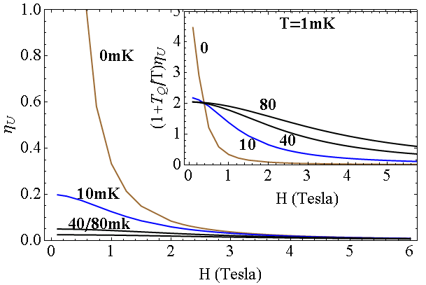
Figure 1: Field-dependent stiffness parameter $\eta_{U}\left(H\right)$ calculated at $T=1$ mK for $T_{Q}=0,10,40,80$ mK. Inset: The hybrid product $\left(1+T_{Q}/T\right)\eta_{U}\left(H\right)$ calculated for the same $T$ and $T_{Q}$ values as presented in the main figure.

A similar hybrid form and limiting behavior at zero temperature characterize the interaction term in the SCF equation (29). The four-electron correlator:

$$\left(F_{U}\left(h\right)\right)_{T\rightarrow 0}=\left(\frac{T}{T_{Q}}\right)_{T\rightarrow 0}F_{Q}\left(h\right)$$ (38)

where:

$$F_{Q}\left(h\right)\equiv\frac{1}{\eta_{Q}\left(h\right)}\int\limits_{0}^{\infty}d\nu\frac{\varkappa_{\nu}^{Q}\left[\left(\varkappa_{\nu}^{Q}\right)^{2}+\mu_{Q}^{2}h^{2}\right]}{\left[\varkappa_{\nu}^{Q}\left(\varkappa_{\nu}^{Q}-2\beta_{Q}\right)+\mu_{Q}^{2}h^{2}\right]^{3}}$$ (39)

shows similar singular behavior to that of $\eta_{U}\left(h\right)$ (see Eqs.(36) and (37)). The overall interaction term has the finite regular limiting form (including the logarithm):

$$\alpha F_{U}\left(h\right)\left(1+T_{Q}/T\right)\ln\left(1+\frac{\eta_{U}\left(h\right)x_{0}t^{-1}}{\widetilde{\varepsilon}_{h}^{U}}\right)$$

$$\rightarrow\alpha F_{Q}\left(h\right)\ln\left(1+\frac{\eta_{Q}\left(h\right)x_{0}}{\widetilde{\varepsilon}_{h}^{Q}t_{Q}}\right)$$ (40)

This SCF approach avoids the critical divergence of both the AL paraconductivity and the DOS conductivity, and allows to extend the expression for the conductance fluctuations $\sigma^{fluct}d=\sigma_{AL}d+\delta\sigma_{DOS}d$, given in terms of Eqs.(III.1),(18), to regions well below the nominal critical SC transition. It also offers an extended proper measure of the pair-breaking effect. In contrast to $\varepsilon$_h, $\widetilde{{\normalsize\varepsilon}}_{h}$ is positive definite in the entire fields range, including that below the critical field where $\varepsilon$${}_{h}<0$ (see Fig.2). The uniform enhancement of $\widetilde{{\normalsize\varepsilon}}$${}_{h}^{U}$ with respect to $\widetilde{{\normalsize\varepsilon}}_{h}$, seen in Fig.2, resulting from the introduction of the frequency shift to the SCF equation (29), is a genuine measure of the pair-breaking effect associated with the quantum tunneling. Its monotonically increasing field dependence seen in Fig.2 properly reflects the field-induced pair-breaking effect in the entire fields range.

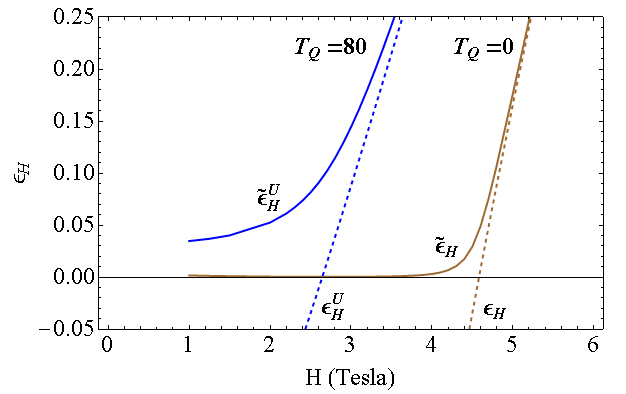
Figure 2: Field dependence, at $T=30$ mK, of the "bare" critical-shift parameter $\varepsilon_{H}^{U}$ (dashed lines), and the corresponding self-consistently "dressed" parameter $\widetilde{\varepsilon}_{H}^{U}$ (solid lines), in the absence of quantum tunneling (brown curves) and for $T_{Q}=80$ mK (blue curves).  Note the downward shift of the critical field and the uniform enhancement of the dressed critical-shift parameter associated with the quantum tunneling effect.

V Discussion

In this paper we have discovered, while searching for the deep origin of the high-field insulating states appearing at diminishing temperature, that due to extreme softening of the fluctuation modes and their redistribution over a large region in momentum space, there is a propensity of Cooper-pair fluctuations to condense in real-space puddles of decreasing spatial size, $\widetilde{\xi}\left(t\rightarrow 0\right)$ (see Eq.(24)). This picture is of course ideal, but basically reflects real tendency toward boson insulating states. Charge transfers between the exclusive bosons system and the normal-electron states, underlying the microscopic Gorkov GL approach employed, are introduced within a unified phenomenological approach, by allowing field-induced pair-breaking processes to develop during dynamical quantum tunneling of Cooper-pair fluctuations out of the mesoscopic puddles.

Other quantum fluctuations effects arising from coherent Andreev-like scattarings Lopatinetal05 , LV05 , ManivAlexander76 , associated with the Maki-Thompson (MT) contribution to the paraconductivity MakiPTP1968 , ThompsonPRB1970 , are expected to be suppressed by strong spin-orbit scatterings LV05 , which characterize the SrTiO₃/LaAlO₃ interfaces under consideration here Mograbi19 , RoutPRL2017 .

Exploiting the complete agreement between the results of our approach and those of the fully microscopic theory at zero magnetic field, it will be meaningful at this point to compare the influence of the quantum fluctuations employed in each approach on the conductivity at finite field. Thus, on one hand, the DOS conductivity derived in our approach in the quantum limit (see Eq.48), and the renormalized single-particle conductivity derived within the fully microscopic approach in the quantum fluctuations regime Glatzetal2011 , are both finite, with negative sign, and have the same field dependence. On the other hand, in the fully microscopic approach the vanishing rate of the AL paraconductivity is further accelerated in the quantum fluctuations regime Glatzetal2011 , whereas in our approach the vanishing AL conductivity (see Eq.(23)) is recovered by the effect of quantum tunneling (see Eq.50). The physical reasoning behind this recovery is explained in Sec.IV and in Appendix B.

An important feature of the localization process predicted in our approach is its dynamical nature, namely that it occurs in response to the driving electric force MZPRB2021 , and not spontaneously in a thermodynamical process toward equilibrium state. This feature seems to distinguish it from the various approaches to the phenomenon of SIT discussed in the literature Dubi07 , Bouadim2011 , GhosalPRL98 , Vinokur2008 , in which disorder-induced spatial inhomogeneity in the form of SC islands is involved in generating the insulating state. However, in a similar manner the formation of fluctuation puddles in our approach is controlled by disorder, which strongly affect the Cooper-pairs amplitude correlation function in real space. This can be seen by comparing the pair correlation function derived in the dirty limit MZPRB2021 ,CaroliMaki67I to that obtained in the pure limit CaroliMaki67II .

Another important parameter in our approach of relevance to the insulating behavior that seems to have a parallel in the literature Bouadim2011 , is the self-consistent critical shift parameter $\widetilde{\varepsilon}_{H}$, which also plays the role of an energy gap in the Cooper-pair fluctuations spectrum MZPRB2021 . Thus, it is interesting to note that the two-particle gap, which characterizes the insulating state in Ref.Bouadim2011 , vanishes at the SIT. Analogously, in our approach the (two-particle) Cooper-pair fluctuation gap $\widetilde{\varepsilon}_{H}$ gradually diminishes to very small (nonvanishing) values upon decreasing field below the sheet-resistance peak (see Fig.2), in accord with the lack of a critical point.

The combined effect of this nonvanishing two-particle gap $\widetilde{\varepsilon}_{H}$ and the diminishing stiffness parameter $\eta\left(H\right)$ upon increasing field at very low temperatures, is responsible for the loss of long-range phase coherence and for the puddles formation. The resulting boson insulating state is reminiscent of the field-induced paired insulating phase discussed in Ref.Datta-arXiv2021 , which is also closely related to the picture of the suppressed Bose insulator deliberated in Ref.BaturinaPRL2007 . The introduction of quantum tunneling of Cooper-pair fluctuations within our complementary phenomenological approach, which leads to the broadening of the sharp MR peaks at low temperatures, is clearly consistent with the conducting Josephson tunneling effect among SC islands.

Finally, a few comments about the robustness of the quantitative comparison with the experimental data Mograbi19 are in order. As the direct analytic continuation scheme of the AL correlator employed in Ref.MZPRB2021 (see the remarks below Eq.(18)) doubles the prefactor of the corresponding paraconductivity as compared to the well-known result, the implication for the fitting process of using the latter prefactor is expected to further amplify the relative magnitude of the negative DOS conductivity and so to further reinforce the appearance of the field-induced boson insulating states at low temperatures. This has been confirmed quantitatively in Appendix D by repeating the fitting process described in detail in Ref.MZPRB2021 with the 1/2 prefactor of the AL contribution. The results show that good agreement with the experimental data can be achieved also with the reduced AL prefactor by changing the spin-orbit scattering parameter moderately within its range of uncertainty.

VI Acknowledgments

We would like to thank Eran Maniv, Itai Silber and Yoram Dagan for useful discussions. We are also indebted to Andrei Varlamov for helpful comments.

Appendix A Range of validity of the linear approximation

Extending the first order expansion to next order, i.e. writing: $\Phi\left(x;\varepsilon_{H}\right)=\varepsilon_{H}+\eta\left(H\right)x+\zeta\left(H\right)x^{2}+...$, where $\zeta\left(H\right)=\left[a_{+}\psi^{\prime\prime}\left(1/2+f_{-}\right)+a_{-}\psi^{\prime\prime}\left(1/2+f_{+}\right)\right]/2$, we find at low temperature ($t\ll 1$) and finite magnetic field, $h>0$, that in addition to Eq.(21), Eq.(22), $\zeta\left(H\right)\rightarrow\zeta_{0}\left(h\right)t^{2}/h^{4}$, where:

$$\frac{1}{h^{4}}\zeta_{0}\left(h\right)=\frac{1}{2}\left[\int\limits_{0}^{\infty}d\nu\frac{\left(1+\beta_{0}/\sqrt{\beta_{0}^{2}-\mu_{0}^{2}h^{2}}\right)}{\left(\nu+\delta_{0}h^{2}+\beta_{0}-\sqrt{\beta_{0}^{2}-\mu_{0}^{2}h^{2}}\right)^{3}}\right.$$

$$\left.+\int\limits_{0}^{\infty}d\nu\frac{\left(1-\beta_{0}/\sqrt{\beta_{0}^{2}-\mu_{0}^{2}h^{2}}\right)}{\left(\nu+\delta_{0}h^{2}+\beta_{0}+\sqrt{\beta_{0}^{2}-\mu_{0}^{2}h^{2}}\right)^{3}}\right]$$

Evaluation of the integral leads to:

$$\zeta_{0}\left(h\right)=\frac{1}{2}\frac{\left(2\beta_{0}+\delta_{0}h^{2}\right)^{2}-\mu_{0}^{2}h^{2}}{\left[\left(2\beta_{0}+\delta_{0}h^{2}\right)\delta_{0}+\mu_{0}^{2}\right]^{2}}$$

so that the relevant expansion at high fields ($h\sim 1$), is:

$$\Phi\left(x;\varepsilon_{h}\right)\rightarrow\varepsilon_{H}+\frac{1}{h^{2}}\eta_{0}\left(h\right)\left(tx\right)+\frac{1}{h^{4}}\zeta_{0}\left(h\right)\left(tx\right)^{2}+...$$ (41)

with the corresponding temperature independent expansion parameter:

$$xt=\frac{\hbar Dq^{2}}{4\pi k_{B}T_{c}^{\ast}}\leq\frac{\hbar Dq_{c}^{2}}{4\pi k_{B}T_{c}^{\ast}}=x_{0}$$

For the experimental situation encountered in Ref.MZPRB2021 the diamagnetic energy term $\delta_{0}h^{2}$ is much smaller than both the spin-orbit energy $\beta_{0}$ and the Zeeman splitting $\mu_{0}h$, implying that the coefficients: $\eta_{0}\left(h\right)\simeq 2\beta_{0}/\mu_{0}^{2},\zeta_{0}\left(h\right)\simeq\left(4\beta_{0}^{2}-\mu_{0}^{2}h^{2}\right)/2\mu_{0}^{4}$, are constant, or nearly constant (since typically $\left(2\beta_{0}\right)^{2}\gg\left(\mu_{0}h\right)^{2}$).

We therefore conclude that the condition for uniform convergence of the expansion is $x_{0}\ll 1$.  In our fitting process we have used the value $x_{0}=0.015$, well within the domain of convergence.

Appendix B The quantum fluctuations corrections to conductivity

In this appendix we outline the physical reasoning behind our phenomenological quantum fluctuations correction to the two ingredients of the conductance fluctuations. Starting with the DOS conductivity we consider the Cooper-pair density, $n_{s}$, given in Eq.(9), with $\left\langle\left|\phi\left(q\right)\right|^{2}\right\rangle$ in Eq.(13). Approximating $7\zeta\left(3\right)\simeq 8.4$ we rewrite:

$$\left\langle\left|\phi\left(q\right)\right|^{2}\right\rangle\simeq 4.2\frac{\left(n_{2D}\lambda_{T}^{2}\right)}{\Phi\left(x;\varepsilon_{H}\right)}$$ (42)

where  $\Phi\left(x;\varepsilon_{H}\right)\simeq\varepsilon_{H}+\eta\left(H\right)x$, $n_{2D}=k_{F}^{2}/2\pi$ is the density of the 2D electron gas and $\lambda_{T}=\sqrt{\hbar^{2}/2\pi m^{\ast}k_{B}T}$ is the thermal wavelength.

The momentum distribution function $\left\langle\left|\phi\left(q\right)\right|^{2}\right\rangle$ measures the number of bosons per wave vector $\mathbf{q}$ in the Cooper-pairs liquid, engaged in equilibrium with a 2D gas of unpaired mobile electrons with a nominal density $n_{2D}$. The prefactor $n_{2D}\lambda_{T}^{2}=\left(1/2\pi^{2}\right)\left(E_{F}\tau_{T}/\hbar\right)$, that is the number of electrons in an area of size equal to the thermal wavelength, is proportional to the characteristic thermal activation time $\tau_{T}=\hbar/k_{B}T$.

The quantum corrections, introduced in the main text, amount to modifying Expression (42) in two steps; in the first, replacing the temperature $T$, appearing in the denominator of the prefactor, with $T+T_{Q}$, and in the second step inserting the effective frequency-shift term $T_{Q}/2T$ to the arguments of the digamma functions in Eq.(7) consistently with the replacement of $\varepsilon_{H}$ with $\varepsilon_{H}^{U}$. The total modification takes the form:

$$\left\langle\left|\phi\left(q\right)\right|^{2}\right\rangle \rightarrow \left\langle\left|\phi_{U}\left(q\right)\right|^{2}\right\rangle=n_{2D}\lambda_{U}^{2}\frac{4.2}{\Phi_{U}\left(x;\varepsilon_{H}^{U}\right)}$$

$$= \frac{2.1}{\pi^{2}}\frac{\left(E_{F}\tau_{U}/\hbar\right)}{\Phi_{U}\left(x;\varepsilon_{H}^{U}\right)}$$

where $\Phi_{U}\left(x;\varepsilon_{H}^{U}\right)\simeq\varepsilon_{H}^{U}+\eta_{U}\left(H\right)x$. The prefactor $n_{2D}\lambda_{U}^{2}$, is the number of electrons in an effective area $\lambda_{U}^{2}=\hbar^{2}/2\pi m^{\ast}k_{B}\left(T+T_{Q}\right)$ that is proportional to the characteristic time, $\tau_{U}$, for both thermal activation and quantum tunneling of Cooper pairs. Thus, increasing the temperature and/or shortening the time $\tau_{Q}$ for quantum tunneling (which also enhance pair breaking by increasing $\Phi_{U}\left(x;\varepsilon_{H}^{U}\right)$), result in larger rate of thermal and/or quantum leakage from puddles of Cooper pairs. The resulting reduction in the number of Cooper-pairs, which occurs versus a corresponding increase in the number of unpaired mobile electrons, would suppress the DOS contribution to the resistance.

The corresponding unified (quantum-thermal (QT)) density (per unit area) of the Cooper-pairs liquid is now evaluated: $n_{s}^{U}=\frac{1}{d}\frac{1}{\left(2\pi\right)^{2}}\int\left\langle\left|\phi_{U}\left(q\right)\right|^{2}\right\rangle d^{2}q=\frac{1}{d}\frac{1}{\left(2\pi\right)^{2}}\int_{0}^{q_{c}^{2}}\pi d\left(q^{2}\right)\left(\frac{2.1E_{F}}{\pi^{2}k_{B}\left(T+T_{Q}\right)}\right)\frac{1}{\Phi_{U}\left(x;\varepsilon_{H}^{U}\right)}$, so that the unified DOS conductivity, $\sigma_{DOS}^{U}=-\left(2n_{s}^{U}e^{2}/m^{\ast}\right)\tau_{SO}$, is given by:

$$\sigma_{DOS}^{U}d\simeq-4.2\left(\frac{G_{0}}{\pi}\right)\int_{0}^{t^{-1}x_{0}}\frac{dx}{\left(1+T_{Q}/T\right)\Phi_{U}\left(x;\varepsilon_{H}^{U}\right)}$$ (43)

For the AL thermal fluctuations conductivity we start with the retarded current-current correlator $Q_{AL}^{R}\left(\Omega\right)$, Eq.(16), which was obtained from the Matsubara correlator $Q_{AL}\left(i\Omega_{\nu}\right)$ following the analytic continuation $i\Omega_{\nu}\rightarrow\Omega$.  The corresponding electrical response function is seen to be proportional to the thermal energy $k_{B}T$.  The effects of quantum tunneling and pair breaking are introduced by adding to the thermal attempt rate $1/\tau_{T}\propto k_{B}T$ the quantum tunneling attempt rate $1/\tau_{Q}\propto k_{B}T_{Q}$ , and by appropriately inserting the effective frequency-shift term $T_{Q}/2T$  into the function $\Phi\left(x+\left|\mu+\nu\right|;\varepsilon_{H}\right)$, as explained in the main text, i.e.:

$$Q_{AL}^{U}\left(i\Omega_{\nu}\right)=k_{B}\left(T+T_{Q}\right)\left(\frac{2e}{\hbar}\right)^{2}\left(\frac{1}{2\pi d}\right)\int\limits_{0}^{x_{c}}xdx\times$$

$$\sum\limits_{\mu=0,\pm 1,\pm 2,....}\frac{\Phi_{U}^{\prime}\left(x+\left|\mu+\nu\right|;\varepsilon_{H}^{U}\right)}{\Phi_{U}\left(x+\left|\mu+\nu\right|;\varepsilon_{H}^{U}\right)}\frac{\Phi_{U}^{\prime}\left(x+\left|\mu\right|;\varepsilon_{H}^{U}\right)}{\Phi_{U}\left(x+\left|\mu\right|;\varepsilon_{H}^{U}\right)}$$

Now, by repeating the procedure employed in deriving Eq.(17), in which the above discrete summation is directly continued analytically, $\nu\rightarrow\hbar\Omega/2\pi ik_{B}T$, and expanded about zero frequency, we arrive at the following expression for the unified QT AL conductivity:

$$\sigma_{AL}^{U}d=\frac{1}{4}\left(\frac{G_{0}}{\pi}\right)\left(1+\frac{T_{Q}}{T}\right)\int\limits_{0}^{t^{-1}x_{0}}\left(\frac{\Phi_{U}^{\prime}\left(x;\varepsilon_{H}^{U}\right)}{\Phi_{U}\left(x;\varepsilon_{H}^{U}\right)}\right)^{2}dx$$ (44)

As indicated in Sec.IIIB below Eq.(18), the common scheme of analytic continuation utilizing the contour integration method for performing the Matsubara summation yields the same result as Eq.(44) but with the prefactor 1/4 replaced with 1/8.

Appendix C The quantum limit

In this appendix we examine the zero-temperature (quantum) limit of the conductance fluctuation analyzed in Appendix B. We begin by studying the field-induced pair-breaking and quantum tunneling of Cooper pairs in this limiting situation.  Consider the unified (quantum-thermal) expression, Eq.(35), for the critical shift parameter $\varepsilon_{h}^{U}$.

Using the asymptotic expansion of $\psi\left(\frac{1}{2}+T_{Q}/2T+f_{\pm}\right)$ for $T_{Q}/T,$ $f_{\pm}\gg 1$, i.e. $\psi\left(\frac{1}{2}+T_{Q}/2T+f_{\pm}\right)\rightarrow\ln\left(T_{Q}/2T+f_{\pm}\right)=\ln\left[\left(T_{Q}+T_{\pm}\right)/2T\right]$, we have:

$$\varepsilon_{h}^{U}\rightarrow\varepsilon_{h}^{Q}=\ln\left(T/T_{c0}\right)-\ln T+$$ (45)

$$a_{+}\ln\left(T_{Q}+T_{-}\right)+a_{-}\ln\left(T_{Q}+T_{+}\right)-\ln 2-\psi\left(1/2\right)$$

where:

$$T_{\pm}\equiv\frac{D\left(de\right)^{2}H^{2}}{\pi k_{B}\hslash}+\frac{\varepsilon_{SO}}{2\pi k_{B}}\pm\sqrt{\left(\frac{\varepsilon_{SO}}{2\pi k_{B}}\right)^{2}-\left(\frac{\mu_{B}H}{\pi k_{B}}\right)^{2}}$$ (46)

In the above expression for $\varepsilon_{h}^{Q}$ (Eq.(45)), the Cooper singular term, $\ln\left(T/T_{c0}\right)$, is exactly cancelled by the logarithmic term arising from the asymptotic expansion of the digamma functions, so that the remaining regular terms are rearranged to yield the following temperature independent expression for ${\normalsize\varepsilon_{h}^{Q}}$:

$${\normalsize\varepsilon_{h}^{Q}\rightarrow a_{+}\ln\left(\frac{T_{Q}+T_{-}}{T_{c0}}\right)+a_{-}\ln\left(\frac{T_{Q}+T_{+}}{T_{c0}}\right)+\ln 2+\gamma}$$ (47)

where $\gamma\approx 0.5772$… is the Euler–Mascheroni constant, and:

$$a_{\pm}=\frac{1}{2}\left(1\pm\frac{1}{\sqrt{1-\left(\mu_{0}/\beta_{0}\right)^{2}h^{2}}}\right)$$

We now turn to the quantum limit of the DOS conductivity, Eq.(43):

$$\int_{0}^{t^{-1}x_{0}}\frac{dx}{\left(1+T_{Q}/T\right)\Phi_{U}\left(x;\varepsilon_{H}^{U}\right)}\approx$$

$$\int_{0}^{t^{-1}x_{0}}\frac{dx}{\left(1+T_{Q}/T\right)\left[\varepsilon_{h}^{U}+\eta_{U}\left(h\right)x\right]}=$$

$$\frac{1}{\eta_{U}\left(h\right)\left(1+T_{Q}/T\right)}\ln\left(1+\frac{\eta_{U}\left(h\right)t^{-1}x_{0}}{\varepsilon_{h}^{U}}\right),$$

so that by going to the limit $T_{Q}/T\rightarrow\infty$, and using Eq.(37), i.e.: $\eta_{Q}\left(h\right)=\frac{1/2+2\beta_{Q}+\delta_{Q}h^{2}}{\left(1/2+\delta_{Q}h^{2}\right)\left(1/2+\delta_{Q}h^{2}+2\beta_{Q}\right)+\mu_{Q}^{2}h^{2}}\approx\frac{2\beta_{Q}}{\beta_{Q}+\mu_{Q}^{2}h^{2}}=\frac{t_{Q}\eta_{0}}{t_{Q}\eta_{0}/2+h^{2}}$,  we arrive at the final temperature-independent expression:

$$\sigma_{DOS}^{Q}d \simeq -4.2\left(\frac{G_{0}}{\pi}\right)\frac{t_{Q}\eta_{0}/2+h^{2}}{t_{Q}\eta_{0}}\times$$ (48)

$$\ln\left[1+\frac{\eta_{0}x_{0}}{\widetilde{\varepsilon}_{h}^{Q}\left(t_{Q}\eta_{0}/2+h^{2}\right)}\right],$$

$$\eta_{0}\left(h\right) \approx \eta_{0}\equiv\frac{2\beta_{0}}{\mu_{0}^{2}},G_{0}=\frac{e^{2}}{\pi\hbar}$$

where $\widetilde{\varepsilon}_{h}^{Q}$ is determined by the SCF equation, Eq.(29), in the quantum limit, i.e.:

$$\widetilde{\varepsilon}_{h}^{Q}=\varepsilon_{h}^{Q}+\alpha F_{Q}\left(h\right)\ln\left[1+\frac{\eta_{0}x_{0}}{\widetilde{\varepsilon}_{h}^{Q}\left(t_{Q}\eta_{0}/2+h^{2}\right)}\right]$$ (49)

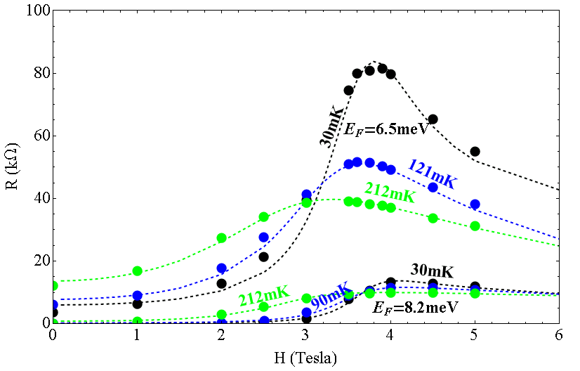
Figure 3: Measured sheet resistance as a function of field at different temperatures for two gate voltages, corresponding to $R_{N}$ $=$ $20.5$ k$\Omega$ ($E_{F}$ $=$ $6.5$ meV) and $7.5$ k$\Omega$ ($E_{F}$ $=$ $8.2$ meV) as reported in Ref.Mograbi19  (full circles). The dashed lines (with temperature labels) represent the results of calculations similar to those performed in Ref.MZPRB2021 , but with 1/2 of the total amplitude of the AL conductivity term used in Ref.MZPRB2021 (see more details in the text of Appendix D).

In the absence of the self-consistent interaction between fluctuations the critical shift parameter reduces to ${\normalsize\varepsilon_{h}^{Q}}$, which vanishes at the quantum critical field ${\normalsize h}_{c}$ , so that near ${\normalsize h}_{c}$:

$${\normalsize\varepsilon_{h}^{Q}\propto h-h}_{c}{\normalsize\rightarrow 0}$$

It is instructive to note that Eq.48 is equivalent to the fluctuation conductivity derived in Ref.Glatzetal2011 in the region of quantum fluctuations within a fully microscopic (diagrammatic) approach.

Considering the unified AL conductivity, Eq.(44) in the linear approximation:

$\sigma_{AL}^{U}d=\frac{1}{4}\left(\frac{G_{0}}{\pi}\right)\left(1+\frac{T_{Q}}{T}\right)\int\limits_{0}^{t^{-1}x_{0}}\left(\frac{\eta_{U}\left(h\right)}{\varepsilon_{h}^{U}+\eta_{U}\left(h\right)x}\right)^{2}dx=\frac{1}{4}\left(\frac{G_{0}}{\pi}\right)\left(1+\frac{T_{Q}}{T}\right)\eta_{U}^{2}\left(h\right)\frac{t^{-1}x_{0}}{\varepsilon_{h}^{U}\left[\varepsilon_{h}^{U}+\eta_{U}\left(h\right)t^{-1}x_{0}\right]}$, so that in the limit, $T_{Q}/T\rightarrow\infty$:

$$\sigma_{AL}^{Q}d\simeq\frac{1}{4}\left(\frac{G_{0}}{\pi}\right)\frac{t_{Q}\eta_{0}^{2}x_{0}}{\left(t_{Q}\eta_{0}/2+h^{2}\right)\widetilde{\varepsilon}_{h}^{Q}\left[\left(t_{Q}\eta_{0}/2+h^{2}\right)\widetilde{\varepsilon}_{h}^{Q}+\eta_{0}x_{0}\right]}$$ (50)

Note that in deriving Eqs.(50), (49) and (48), with the field independent parameter $\eta_{0}$, the small diamagnetic energy term was neglected.

Appendix D Robustness of the fitting process

In this appendix we present results (see Fig.3) of a fitting process similar to that presented in Ref.MZPRB2021 , in which the prefactor of the AL conductivity term is 1/2 of that used in Ref.MZPRB2021 . The level of agreement between these calculations and the experimental data is preserved if the values of the dimensionless spin-orbit scattering parameter used in Ref.MZPRB2021 , i.e. $\beta_{0}=14$ ($R_{N}=7.5$ k$\Omega$) and $\beta_{0}=11$ ($R_{N}=20.5$ k$\Omega$), are changed in the new fitting to $\beta_{0}=16$ and $\beta_{0}=12$ respectively. The phenomenological parameters determining the quantum tunneling attempt rates and the normal state conductivity should also slightly modified. All the other parameters of microscopic origins can remain fixed.

References

• (1) T. Maniv and V. Zhuravlev, "Superconducting fluctuations and giant negative magnetoresistance in a gate-voltage tuned two-dimensional electron system with strong spin-orbit impurity scattering", Phys. Rev. B 104, 054503 (2021).
• (2) A. Ohtomo, and H. Y. Hwang, "A high-mobility electron gas at the LaAlO3/SrTiO3 heterointerface", Nature 427, 423 (2004).
• (3) A. D. Caviglia, S. Gariglio, N. Reyren, D. Jaccard, T. Schneider, M. Gabay, S. Thiel, G. Hammerl, J. Mannhart and J.-M. Triscone, "Electric field control of the LaAlO3/SrTiO3 interface ground state", Nature (London) 456, 624 (2008).
• (4) M. Mograbi, E. Maniv, P. K. Rout, D. Graf, J. -H Park and Y. Dagan, "Vortex excitations in the Insulating State of an Oxide Interface", Phys. Rev. B 99, 094507 (2019).
• (5) S. Ullah and A.T. Dorsey, "Critical Fluctuations in High-Temperature Superconductors and the Ettingshausen Effect", Phys. Rev. Lett. 65, 2066 (1990). Properties of (111) LaAlO3/SrTiO3", Phys. Re. Lett. 123, 036805 (2019).
• (6) S. Ullah and A.T. Dorsey, "Effect of fluctuations on the transport properties of type-II superconductors in a magnetic field", Phys. Rev. B 44, 262 (1991).
• (7) L. G. Aslamazov and A.I. Larkin, Phys. Lett. A 26 p. 238 (1968).
• (8) A. Larkin and A. Varlamov, "Theory of fluctuations in superconductors", Oxford University Press 2005.
• (9) P. Fulde and K. Maki, "Fluctuations in High Field Superconductors", Z. Physik 238, 233–248 (1970).
• (10) T. Maniv and V. Zhuravlev, Unpublished results. It is shown that for frequencies in the region $\Omega<2\pi k_{B}T/\hbar$ the analytic continuation $i\Omega_{\nu}\rightarrow\Omega\rightarrow 0$ directly from the discrete Matsubara sum Eq.(16) is by a factor of 2 larger than that obtained by using the common contour-integration scheme consisting of three sub-contours as done, e.g. in LV05 . Employing the contour-integration scheme for $i\Omega_{\nu}\rightarrow\Omega\rightarrow 0$ with only two sub-contours, i.e. by excluding the intermediate sub-contour, one recovers the result obtained within the direct analytic continuation.
• (11) Estimation of the argument of the logarithmic factor in Eq.(23) just above the "nominal" critical field $H_{c\parallel 0}^{\ast}=4.5$T ($\varepsilon_{h\gtrsim 1}=0.05$) in the $t\rightarrow 0$ limit, based on typical values of our fitting parameters yields $\left(\eta_{0}\left(h\right)x_{0}/h^{2}\varepsilon_{h}\right)_{h\gtrsim 1}\approx 1.3$.  Estimations of the field-dependent prefactors of the AL and the DOS conductivities under the same conditions yield, respectively: $\left(\eta_{0}\left(h\right)/4h^{2}\right)_{h=1}\simeq\left(3.5\zeta\left(3\right)h^{2}/\eta_{0}\left(h\right)\right)_{h=1}\simeq 1$.
• (12) V. M. Galitski and A. I. Larkin, "Superconducting fluctuations at low temperature", Phys. Rev. B 63, 174506 (2001).
• (13) A. Glatz, A. A. Varlamov, and V. M. Vinokur, "Fluctuation spectroscopy of disordered two-dimensional superconductors", Phys. Rev. B 84, 104510 (2011).
• (14) N. Shah and A. V. Lopatin, "Microscopic analysis of the superconducting quantum critical point: Finite-temperature crossovers in transport near a pair-breaking quantum phase transition", Phys. Rev. B 76, 094511 (2007).
• (15) A. V. Lopatin, N. Shah, and V. M. Vinokur, "Fluctuation Conductivity of Thin Films and Nanowires Near a Parallel-Field-Tuned Superconducting Quantum Phase Transition", Phys. Rev. Lett. 94, 037003 (2005).
• (16) T. Maniv and S. Alexander, "Superconducting fluctuation effects on the local electronic spin susceptibility", J. Phys. C: Solid State Phys. 9, 1699 (1976).
• (17) K. Maki, "The Critical flucluation of the Order Paralneter in Type-II Supcreonductors", Prog. Theor, Phys. 39, 897; ibid. 40, 193 (1968).
• (18) R. S. Thompson, "Microwave, Flux Flow, and Fluctuation Resistance of Dirty Type-II Superconductors", Phys. Rev. B 1, 327 (1970).
• (19) P. K. Rout, E. Maniv, and Y. Dagan, "Link between the Superconducting Dome and Spin-Orbit Interaction in the (111) LaAlO3/SrTiO3 Interface", Phys. Rev. Lett. 119, 237002 (2017).
• (20) Y. Dubi, Y. Meir and Y. Avishai, "Nature of the superconductor–insulator transition in disordered superconductors", Nature 449, 876 (2007).
• (21) K. Bouadim, Y. L. Loh, M. Randeria and N. Trivedi, "Single- and two-particle energy gaps across the disorder-driven superconductor–insulator transition", Nature Phys. 7, 884 (2011).
• (22) A. Ghosal, M. Randeria, and N. Trivedi, "Role of Spatial Amplitude Fluctuations in Highly Disordered s-Wave Superconductors", Phys. Re. Lett. 81, 3940 (1998).
• (23) V. Vinokur, T. I. Baturina, M. V. Fistul, A. Yu. Mironov, M. R. Baklanov and C. Strunk, "Superinsulator and quantum synchronization", Nature 452, 613 (2008).
• (24) C. Caroli and K. Maki, "Fluctuations of the Qrder Parameter in Type-II Superconductors. I. Dirty Limit", Phys. Rev. 159, 306 (1967).
• (25) C. Caroli and K. Maki, "Fluctuations of the Qrder Parameter in Type-II Superconductors. II. Pure Limit", Phys. Rev. 159, 316 (1967).
• (26) Anushree Datta, Anurag Banerjee, Nandini Trivedi, and Amit Ghosal, "New paradigm for a disordered superconductor in a magnetic field", arXiv:2101.00220 [cond-mat.supr-con].
• (27) T. I. Baturina and C. Strunk, M. R. Baklanov and A. Satta, "Quantum Metallicity on the High-Field Side of the Superconductor-Insulator Transition", Phys. Rev. Lett. 98, 127003 (2007).