Abstract

In this work, Transition Probability Matrix (TPM) is proposed as a new method for extracting the features of nodes in the graph. The proposed method uses random walks to capture the connectivity structure of a node’s close neighborhood. The information obtained from random walks is converted to anonymous walks to extract the topological features of nodes. In the embedding process of nodes, anonymous walks are used since they capture the topological similarities of connectivities better than random walks. Therefore the obtained embedding vectors have richer information about the underlying connectivity structure. The method is applied to node classification and link prediction tasks. The performance of the proposed algorithm is superior to the state-of-the-art algorithms in the recent literature. Moreover, the extracted information about the connectivity structure of similar networks is used to link prediction and node classification tasks for a completely new graph.

Keywords: Graph representation learning, Feature learning, Link prediction, Node classification, Anonymous random walk.

1 Introduction

The network concept is a mathematical model of structures where elements, the nodes, are connected through the edges. Network connections are because of semantic or geometric relations among the nodes. Entities of complex networks, such as individuals, molecules, neurons, and computers, are represented by nodes, while their relations or interactions make up the edges. These structures, the networks, are observed in diverse areas, and they are primary mathematical tools for modeling complex systems [1, 2]. Common properties of complex systems, such as clustering [3], forming communities [4], and new links [5] are all in the interest of researchers of different disciplines, as the common network structures are observed in diverse areas, such as physical, biological, and social sciences. For this reason, networks have opened new opportunities for a better understanding of the underlying dynamics of diverse problems of ever-growing complexity. Moreover, new challenges appear as the sizes of the networks and the complexity of the problems of interest increase. The challenges are manifold. Among various challenges in data mining, getting the correct picture of the relations in large networks profoundly exhibits itself. The problems related to network mining, such as community detection [6, 7], node classification [8], link prediction [9], structural network analysis [10], and network visualization [11], are being studied.

Nodes in complex networks carry highly structured information. Considerable effort has been devoted to processing this information over the last few years. The issue is to correctly identify the feature vector representation of the nodes and edges. Old-fashioned traditional solutions offer hand-engineering through expert knowledge. Because this is for special cases, it is challenging to generate different tasks. For this purpose, various graph embedding approaches  [12] have been introduced. Graph embedding is a map between high-dimensional, highly structured data and low-dimensional vector space that preserves the structural information of all nodes in the network. The embedding process gains importance due to the growing number of applications that benefit from network data in a broad range of machine learning domains, such as natural language processing (NLP), bioinformatics [13], social network analysis [14, 15], and recently as building blocks of reinforcement learning algorithms [16, 17].

In-network-related problems, node classification, finding relations, and predicting non-apparent connections among the entities are the crucial steps for approaching the problem. Hence, the extraction of implicit information present in the network and identifying the existing links is the base requirement of all network-related problems. The link prediction comprises inferring the existence of connections between network entities based on the properties of the nodes and observed links [18]. The purpose is to label an unlabeled node by evaluating a labeled node. In a link prediction task, the purpose is to predict a possible link between two nodes by considering the existing links in the network. The techniques designed to solve node classification and link prediction problems are also used in modeling new networks and predicting network evolution mechanisms [19, 20].

It is common practice in social networks and recommendation systems that two entities with similar interests are more likely to interact. Hence, commonly shared empirical evidence shows that similar nodes are likely to interact. Palla et al. [21] observed that nodes tend to form connected communities. This observation has led to an accepted similarity definition as the amount of relevant direct or indirect paths between nodes. Therefore the challenge in node identification and link prediction is to define similarities in network entities. The nodes carry geometric identities, which are the reflections of network topology. Besides these topological characteristics, some networks also provide homophily identities for the nodes. This information has applicability among a wide range of different networks. A better understanding of the network domain and the existence of semantic information together with the geometric connectivity helps define the node similarity and increases the learning algorithm’s efficiency.

In node classification and link prediction, two main obstacles are the lack of information and the size of the real-world networks. Real-world networks consist of millions of nodes, and the number of links is a large multiple of the number of nodes. For such large structures, only geometric information may not be sufficient for node identification. This is particularly true in very sparse networks. The remedy, found in some algorithms, is to extend the network region surrounding the node. More sites are included in the information-gathering process by increasing the region to collect information. Here another bottleneck comes into play. Such algorithms are computationally expensive and can only apply to small networks. The amount of information collected from the network, the algorithm’s complexity, and the techniques to collect information must be balanced.

This work introduces a new scalable unsupervised node embedding algorithm to calculate the transition probability between the neighboring sites. The transition probability carries the characteristic connectivity structure of the region around the node in concern. The idea is to capture the local connection structure of a node by visiting a few close neighbors. This approach saves computation time, increases performance, and enables information collection without going deep into a graph. This is achieved by starting a random walk from each node in a predefined number of steps. Then random walks are converted into anonymous walks to extract the variety and richness of connections around the nodes. This approach focuses on capturing the neighboring structural patterns rather than the node’s identity. These anonymous walks preserve the local structural information and are used in calculating the transition probability matrix (TPM) elements. The transition probability matrix defines the probability of being in neighboring nodes at each time step. The transition matrix elements include the probability of reaching the predecessor, new, or already visited node at each time step. This information creates a fingerprint of how dense or sparse local ties are.

In the proposed work, the elements of the transition probability matrix are used as feature vectors for each node. The TPM method makes two main contributions to the literature. The first is to produce a feature vector representation using an anonymous walk and offer a new embedding method. The second one is to use this extracted information from sample networks in a new network with a similar topological connectivity structure. The idea is to use the similarity of connections without considering the node’s details. In traditional classification problems, data is used to train the algorithm, and predictions are made on the same network, of which information is already used as a part of training data. To the best of our knowledge, the proposed algorithm is the first in the literature to test the performance of the embedding process on a completely different graph except for having the same topological connectivity structure. The power of the proposed algorithm comes from the generality of the local connectivities, demonstrating the similarity of the topological structures of the networks. Hence, structural equivalence (roles of nodes in the network) dominates the unavailable features to find the similarities needed for classification and prediction tasks. Nodes’ inner structures or identifications are hidden in many real-world cases. So it is essential to use topological features in the embedding process. Despite being unique to a node in the given network, the topology of the real-world networks allows the node feature vector to be used in different similar networks for prediction. In this sense, the proposed algorithm exhibits possibilities for various applications. The possibility of obtaining information from a similar network for predictions on the new networks is the most general characteristic that makes the proposed algorithm superior to random walks or graph convolutional network-based models for many real datasets.

The rest of the paper is organized as follows: the next section briefly describes the proposed embedding algorithm TPM. In Section 3, we experimentally test TPM on various network analysis tasks over three citation networks and examine the parameter sensitivity of our proposed method. Finally, our conclusions and future works are presented in section 4.

2 Model

Networks are mathematically represented by graphs $G(V,E)$. Graphs consist of a set of nodes ($V$) and edges ($E$) connecting nodes. Assuming no multiple connections exist among the nodes, a network of $N$ nodes can have at most $E_{Max}=N(N-1)/2$ undirected edges. Here, $E_{Max}$ is the maximum number of possible connections. The network structure with $E_{Max}$ connections is called "fully connected". Apart from the fully connected networks, all network topologies possess a number of connections less than $E_{Max}$. For any specific network, its topology limits the number of edges. Apart from the fully connected networks, each network has a characteristic pattern of connections around the vertices, making classification of the network topology possible. Depending on degree distribution, there are mainly different connectivity structure power law (scale-free) and Erdos-Renyi (Random) networks.

The set of known edges $E$ is considered positive (existent), while the set $E_{Max}-E$ edges constitute the set of non-existent edges and are called negative edges. The unique local connectivity structure of the given network plays the most crucial role in node characterization. Node features are representations of relations among the sites in a given neighborhood radius. At this point, there exist different recipes and methods of node feature extraction ([22] for a survey). Different feature extraction algorithms determine the features of a given node with relative success, computational complexity, and computational expense. The success in determining the features of the nodes is essential since it is used as an input for more complicated constructions, such as the process of link prediction and community detection. The link prediction is an identification process of the possible candidates of positive edge sets in the set of non-existing edges, $E_{Max}-E$. The prediction process proceeds by assigning weights, $w_{i,j}$ to all possible edges between the nodes, labeled $n_{i}$ and $n_{j}$. Weights are model-defined similarity relations between the neighboring nodes. The relations are determined by the rules based on the features of the nodes. The possible positive edges are predicted according to their weight values; the higher the score, the more likely an edge exists.

The node feature extraction algorithms commonly employ random walks. Notably, highly cited DeepWalk [23] and node2vec [24] methods base their feature extraction algorithms on creating large sequences of random walks, in a similar setting to sentences in natural language processing. Words and sentences correspond to nodes and random walks, respectively. The relational information between the node in concern and neighboring nodes is obtained from random walk sequences. Apart from these two well-established algorithms, a new, random walk-based approach for learning entire network representation has been introduced [25] recently. In this new approach, random walks are converted to anonymous walk sequences by relabeling nodes by their occurrences in the walk.

In the present work, anonymous walks are a good candidate for extracting topological features of the whole network and are used to extract feature vectors of the nodes. The proposed method showed that learning the node representation is possible by extracting local connectivity information as node features via anonymous walks.

2.1 Anonymous Random Walks

An anonymous random walk is a process of relabelling the nodes. In a local random walk sequence, nodes are labeled according to their occurrence to obtain an anonymous walk sequence. A random walk of length $m$ starting from the node $v_{i}$ is a set of node labels, $R_{w}=(v_{1},v_{2},\dots,v_{m})$ where all $v_{i}\;\in\;V$. The anonymization process is a mapping between the actual node labels and their occurrences in the sequence, $A_{w}=(f(v_{1})\dots,f(v_{m}))$. This anonymization process provides encapsulated information to reconstruct the local structure of the graph without requiring global node labels. Micali & Zhu [26] have shown that by using anonymous random walks of length, $m$, starting from a node $v_{i}$ are used to reconstruct the immediate neighborhood of the node $v_{i}$. Therefore, using anonymous random walks, local topological features of nodes provide consistent information to construct a global structure of the graph.

2.2 Problem Formulation

The behavior of the random walks represents the local connectivity structure of any node $v_{i}$. The random walk sequences contain new nodes at almost every step if the region is loosely connected. The probability of returning to the already visited sites increases if the neighborhood is densely connected. This information gives a unique picture of the connectivity structure near node $v_{i}$. Therefore, the transition probability is a good candidate for the extraction of the topological features of the nodes. The proposed algorithm aims to extract a map of the local topological structure of a given node using the transition probability. The proposed node embedding is based on calculating transition probability from any node within a certain number of steps around the node $v_{i}$. The probability of reaching a neighboring node is proportional to the degree of the node in concern. Hence, from a set of anonymous random walks, all starting from node $v_{i}$, the obtained distribution of reaching a new node or moving back to one of the already visited nodes at a given time step constitutes the elements of the transition matrix. The feature embedding vector of a node $v_{i}$ is the transition probability matrix obtained from the transition matrix.

2.3 Obtaining Transition Matrix-Conceptual Considerations

Using random walks makes it possible to obtain a sequence of nodes in the graph. The positions of the nodes in this sequence will be related to the connectivity structure of the graph and keep rich information about the local neighborhood. The more distance we travel through the graph, the more global information we obtain. Local connectivity structure and variety of neighbors of any node are significant for some tasks, graph recovery, reconstructing topology [26, 27], etc. For this reason, a limited length of random walks $m$ starts from each node is done and converted to $m$ step anonymous walks. The initial node, $v_{i}$, is considered the zeroth node, $a_{0}$, in the anonymous walk. The next node in the sequence is one of the nearest neighbors of node $v_{i}$, reached in the first step of the random walk. Each neighbor of $v_{i}$ has the same probability of being visited, which is related to the degree ($d_{i}$) of $v_{i}$. The same process continues for the next steps of random walks, so the underlying topological structure of the neighborhood of the visited nodes is embedded into the details of the next step.

In principle, depending on the connectivity structure of one of the previously visited nodes, a new unvisited node or previous node can be reached at the next step. The only condition to reach any previously visited node in the next steps is to have a direct connection to that node. Hence, the high probability of reaching an already visited node is an indication of the densely connected local region.

Let a random walk $R_{w}=(v_{1},v_{2},\dots,v_{m})$ where all $v_{i}\;\in\;V$. The corresponding anonymous walk is obtained by calculating the position of each node in the walk. So if an already visited node is visited at any step of the walk, the position index value that appears for the first time is used [25].

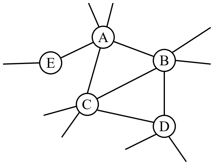
Figure 1: Sample subgraph.

In this sample graph (Figure 1), let’s start a set of random walks with length $4$ from node $A$ and convert them to anonymous walks.

$R_{w1}:A\rightarrow B\rightarrow C\rightarrow A\rightarrow E\hskip 50.00008ptA_{w1}:a_{0}\rightarrow a_{1}\rightarrow a_{2}\rightarrow a_{0}\rightarrow a_{3}$

$R_{w2}:A\rightarrow C\rightarrow D\rightarrow C\rightarrow A\hskip 50.00008ptA_{w2}:a_{0}\rightarrow a_{1}\rightarrow a_{2}\rightarrow a_{1}\rightarrow a_{0}$

$R_{w3}:A\rightarrow B\rightarrow D\rightarrow B\rightarrow A\hskip 50.00008ptA_{w3}:a_{0}\rightarrow a_{1}\rightarrow a_{2}\rightarrow a_{1}\rightarrow a_{0}$

The corresponding anonymous walks have information about the variety of neighbors and topological structures. For this reason, it is possible that two different random walks ($R_{w2}$ and $R_{w3}$) can produce the same anonymous walks. In a random walk for the next step to move, there are mainly three different possibilities:

1. $P_{new}$     visit a new node.

2. $P_{prev}$     visit (go back) to previous node.

3. $P_{already}$     visit an already visited node.

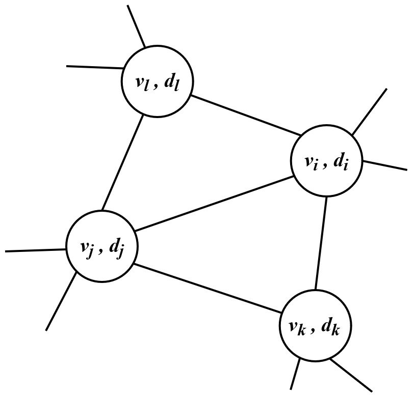
Figure 2: Sample subgraph, $d_{i}$ is degree of node $V_{i}$.

For a random walk starts from node $v_{l}$ in Figure 2, let’s assume that first step is node $v_{i}$ and the second step is node $v_{j}$ ($v_{l}\rightarrow v_{i}\rightarrow v_{j}$). For the next step, possible choices are:

$P_{j,k}$     to a new node

$P_{j,i}$     to a previous node

$P_{j,l}$     to an already visited node

Let $P^{t}_{i,j}$ be the transition probability from node $i$ to node $j$ at time step $t$. Considering a three-step random walk. The possible sequence of the anonymous walk is,

At step 0	with	$P=1$	be in node $a_{0}$	$a_{0}$
At step 1	with	$P^{(1)}_{new}$	be in node $a_{1}$	$a_{0}\rightarrow a_{1}$
At step 2	with	$P^{(2)}_{prev}$	be in node $a_{0}$	$a_{0}\rightarrow a_{1}\rightarrow a_{0}$
	with	$P^{(2)}_{new}$	be in node $a_{2}$	$a_{0}\rightarrow a_{1}\rightarrow a_{2}$
At step 3	with	$P^{(3)}_{prev}$	be in node $a_{0}$	$a_{0}\rightarrow a_{1}\rightarrow a_{0}\rightarrow a_{1}$
if $P^{(2)}_{prev}==1$	with	$P^{(3)}_{new}$	be in node $a_{2}$	$a_{0}\rightarrow a_{1}\rightarrow a_{0}\rightarrow a_{2}$
if $P^{(2)}_{new}==1$	with	$P^{(3)}_{prev}$	be in node $a_{1}$	$a_{0}\rightarrow a_{1}\rightarrow a_{2}\rightarrow a_{1}$
	with	$P^{(3)}_{new}$	be in node $a_{3}$	$a_{0}\rightarrow a_{1}\rightarrow a_{2}\rightarrow a_{3}$
	with	$P^{(3)}_{already}$	be in node $a_{0}$	$a_{0}\rightarrow a_{1}\rightarrow a_{2}\rightarrow a_{0}$

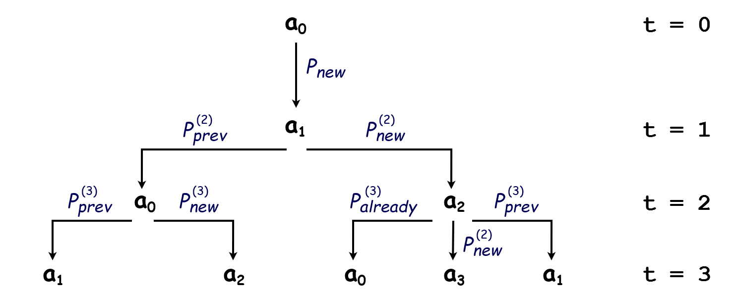
Figure 3: Shows the probabilities of visiting nodes in a three-step neighborhood.

The tree-like representation shows the visiting probabilities of the nodes in the 3-step neighborhood (Figure 3). The probabilities of arriving nodes at each time step are summed to calculate the elements of the transition probability matrix for each node. The calculated probabilities for a three-step anonymous random walk are presented in Table 1 to exemplify the idea. The Transition probability matrix, TPM, obtained for a three-step anonymous walk can be given as in Table 2.

Step		Probability	Node
$1$	$P^{(1)}_{0,1}$	$\frac{1}{d_{0}}$	$0\;\rightarrow\;1$
$2$	$P^{(2)}_{1,0}$	$P^{(1)}_{0,1}\times\frac{1}{d_{1}}$	$1\;\rightarrow\;0$
	$P^{(2)}_{1,2}$	$P^{(1)}_{0,1}\times\frac{d_{1}-1}{d_{1}}$	$1\;\rightarrow\;2$
$3$	$P^{(3)}_{2,0}$	$P^{(2)}_{1,2}\times\delta_{2,0}\times\frac{1}{d_{2}}$	$2\;\rightarrow\;0$
	$P^{(3)}_{2,1}$	$P^{(2)}_{1,2}\times\frac{1}{d_{2}}$	$2\;\rightarrow\;1$
	$P^{(3)}_{2,3}$	$P^{(2)}_{1,2}\times\left[\frac{d_{2}-2}{d_{2}}+[1-\delta_{2,0}]\times\frac{1}{d_{2}}\right]$	$2\;\rightarrow\;3$
	$P^{(3)}_{0,1}$	$P^{(2)}_{1,0}\times\frac{1}{d_{0}}$	$0\;\rightarrow\;1$
	$P^{(3)}_{0,2}$	$P^{(2)}_{1,0}\times\delta_{0,2}\times\frac{1}{d_{0}}$	$0\;\rightarrow\;2$
	$P^{(3)}_{2,3}$	$P^{(2)}_{1,0}\times\left[\frac{d_{0}-2}{d_{0}}+[1-\delta_{0,2}]\times\frac{1}{d_{0}}\right]$	$2\;\rightarrow\;3$

Table 1: Anonymous random walk probabilities for a set of three-step anonymous walks. Theoretical probability values describe the probabilities of the vicinity of the neighbors at each time step. Here $d_{i}$ is the degree of each node and $\delta_{i,j}$ is the Kronecker delta, which indicates the connection between node $v_{i}$, and node $v_{j}$.

		$a_{0}$	$a_{1}$	$a_{2}$	$a_{3}$
		1	0	0	0		$t=0$
		0	$P^{(1)}_{0,1}$	0	0		$t=1$
$TPM=$		$P^{(2)}_{1,0}$	0	$P^{(2)}_{1,2}$	0		$t=2$
		$P^{(3)}_{2,0}$	$P^{(3)}_{0,1}+P^{(3)}_{2,1}$	$P^{(3)}_{0,2}$	$P^{(3)}_{2,3}$		$t=3$

Table 2: Transition probability matrix element for each time step.

2.4 Obtaining Transition Matrix - Implementation

The above transition probability matrix (Table 2) is obtained from a given graph by creating a set of random walks starting from each network node. The elements of the probability matrix are obtained by counting the number of anonymous random walk sequences, which means how many times each node is visited at each time step.

$$d_{i,j}=\sum_{k}\delta(A^{(k)}_{i,j},j)$$ (1)

This process provides a distribution matrix for each node. The obtained distributions are normalized to obtain transition probability matrices. The algorithm 1 illustrates the process of creating a set of anonymous random walks and obtaining the transition probability matrix.

Input:

          Graph $G(V;E)$

          Walks per node $\eta$

          Walk length $m$

Output: Node representation $X(v)$ for each node $v\in V$

1

2for each $v\in V$ do

       Initialize $walks_{v}$ to Empty

        // Random walks set

       Initialize $anons_{v}$ to Empty

        // Anonymous random walks set

       Initialize $tpm_{v}=[t]_{|m+1|\times|m+1|},t=0$

        // Transition probability matrix

3       for $i=0$ to $\eta$ do

4             $w=$ UniformlyRandomWalk$(G,v,m)$

5             Append a walk $w$ to $walks_{v}$

6      $anons_{v}=$ AnonymousRandomWalk$(walks_{v},v,m)$

7       $k=0$

      // Go through the steps of the anonymous random walks

8       for $step$ in $anons_{v}$ do

             // Count the number of visited node at each step of the walk

9             Update $tpm_{v}[k,step]$ $+$= 1

10             Update $k$ $+$= 1

11      $X(v)=normalize(tpm_{v})$

Return $X$

Algorithm 1 Methodology of Creating Transition Probability Matrix

Once the transition probability is obtained for each node, the transition probability matrix may be used in various ways for calculating the network properties. In this work, the aim is to show how well the local characteristics of a given node are preserved in the definition of the transition probability matrix. To this end, it is used as node features in node classification, link prediction, visualization, and cross-networks generalization tasks. The implementation of the embedding process consists of four steps (Please see, Figure 4):

1. Create a set of random walks, $\eta$ with length $m$ starting from each node.

2. Convert each random walk to an anonymous walk.

3. Calculate the distribution matrix ($|m+1|\times|m+1|$) for each node.

4. Obtain the Transition Probability Matrix (TPM, $|m+1|\times|m+1|$ matrix) for each node after normalizing the distribution matrix from the previous step.

5. Use TPM as node features in the embedding process.

Here $m$ refers to the number of steps in a random walk. Because the purpose is to collect the local information about a node, a high number of steps causes it to go too deep into the graph.

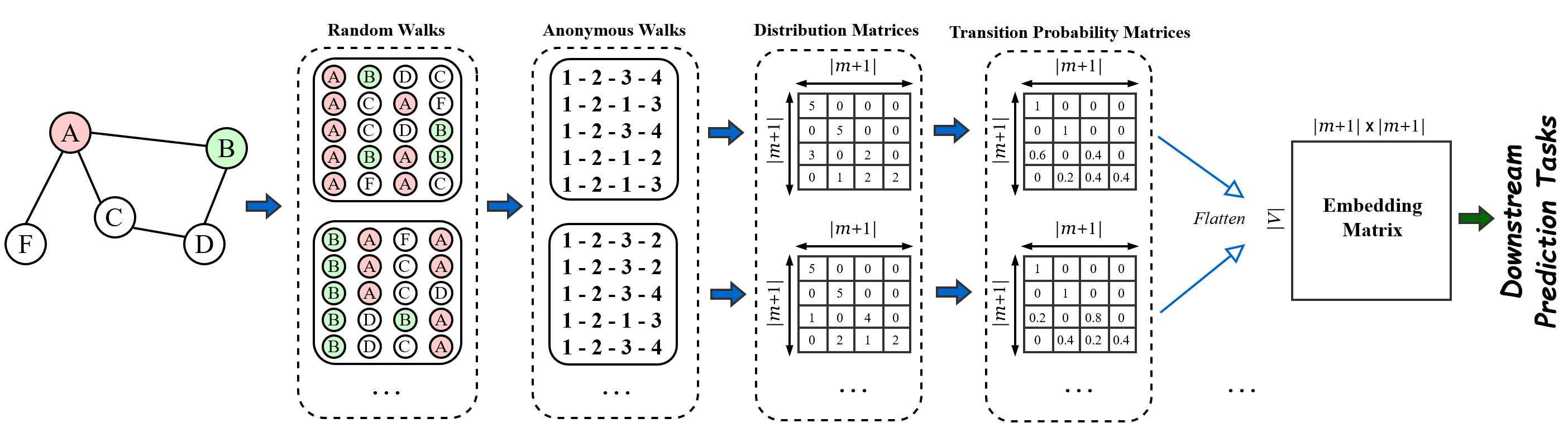
Figure 4: Architecture of the TPM model

3 Experiments

The proposed method (TPM) is compared against numerous state-of-the-art baseline embedding techniques on four downstream tasks: node classification, link prediction, network visualization, and cross-networks generalization. In addition, parameter sensitivity is conducted. The results demonstrate that our method considerably outperforms the baseline embedding techniques in all the network analysis tasks.

3.1 Datasets

Three different citation networks are employed to test the quality of the proposed embedding method (TPM). Table 3 shows the network statistics of Cora [28], Citeseer [29], and Pubmed [30] networks, which are commonly used for testing algorithms and predicting network properties in a considerable number of publications [31, 32, 33, 34]. Cora, Citeseer, and Pubmed comprise academic publications, which are the nodes, and citation relations between papers, which are the edges. Each node is labeled according to its research field. All of the datasets are open to the public .

Table 3: Overview of three citation networks datasets.

	Cora	CiteSeer	Pubmed
Nodes	2,708	3,327	19,717
Edges	5,429	4,732	44,338
Classes	7	6	3

3.2 Baselines

We compare the performance of our proposed TPM model with six well-established feature extraction algorithms (DeepWalk [23], node2vec [24], LINE [35], GCN-Graph Convolutional Network [36], GraphSAGE [37], and GAT [38]).

• DeepWalk [23] is an unsupervised approach that learns low-dimensional representations of nodes by using local structural information collected from truncated random walks.

• node2vec [24] proposes a more flexible strategy (biased random walks) for sampling node sequences, which allows it to better balance the importance of the local and global structure of a graph.

• LINE [35] optimizes a predefined objective function in a way that maintains the network topology on both the local (first-order proximity) and the global (second-order proximity) levels. For each node, LINE computes two feature representations and then utilizes an efficient method to combine the vector representations learned by LINE (first-order) and LINE (second-order) into a single, $d$-dimensional vector.

• GCN-Graph Convolutional Network [36] is a widely common form of Graph Neural Networks (GNNs). In GCN, the representation of each node is created by a convolution layer that aggregates both the node’s attributes and the attributes of its surrounding nodes. The success of the GCN is attributable to two techniques: first, the adjacency matrix is normalized by the degrees, and second, each node is given a self-connection.

• GraphSAGE [37] is the pioneering inductive framework, and it uses the concept of spatial GCN-Graph Convolutional Network to learn node representations. Essentially, it creates an aggregation function (might be mean (as in GCN), pooling, or LSTM) to collect attributes from each node’s neighbors.

• GAT [38] combines techniques of attention with Graph Neural Networks (GNN) in an effort to improve its learning capability in relation to the characteristics of neighborhoods.

According to the relevant literature, these baselines have exhibited state-of-the-art embedding performances on the datasets used in our tests. As for parameter settings, the number of walks per node, length of walks, window size, and negative sampling are set to 10, 80, 30, and 10 for both DeepWalk and node2vec, respectively. We observed experimentally that setting $p=2$ and $q=1$ in node2vec produces superior results across all datasets. We used the recommended hyperparameters and default architectures for the rest baseline methods based on the corresponding original papers. We set the number of walks per node $\eta=20$ and the length of walks $m=10$ for our proposed (TPM) model. For the sake of fair comparison, the representational dimension ($d$) for all baselines has been fixed to 128.

3.3 Evaluation Metrics

As evaluation metrics, we use Macro-F1 and Micro-F1 scores [39] for the node classification task, and we use AUC (area under the ROC curve) [40] for the link prediction task. Higher values of these metrics indicate better performance of the related network embedding technique.

• Macro-F1 is the mean of the per-class F1 scores.

• Micro-F1 calculates a global average F1 score by adding the total number of True Positives (TP), False Negatives (FN), and False Positives (FP) across all labels.

The formulas of Macro-F1 and Micro-F1 are:

$$\text{ Macro-F1}=\frac{1}{c}\sum_{i=1}^{c}\frac{2TP_{i}}{2TP_{i}+FP_{i}+FN_{i}}$$ (2)

$$\text{ Micro-F1}=\frac{2\sum_{i=1}^{c}TP_{i}}{\sum_{i=1}^{c}2TP_{i}+FP_{i}+FN_{i}}$$ (3)

where $c$ denotes the number of classes.

• Area under the ROC curve, or AUC, is the probability that the score of a positive link (existent) is greater than the score of a randomly selected link that does not exist. AUC compares $n$ times the scores of a randomly picked positive (existent) and negative (nonexistent) link. If $n^{\prime}$ times an existent link’s score is greater than a nonexistent link’s, and $n^{\prime\prime}$ times they share the same score, the AUC is:

$$\text{ AUC}=\frac{n^{\prime}+0.5n^{\prime\prime}}{n}$$ (4)

Table 4: Summary of node classification results. Bold values mean the best results.

	CORA		CiteSeer		Pubmed
	Micro-F1	Macro-F1	Micro-F1	Macro-F1	Micro-F1	Macro-F1
DeepWalk	0.715	0.692	0.560	0.521	0.659	0.652
node2vec	0.846	0.838	0.751	0.703	0.722	0.717
LINE	0.797	0.793	0.582	0.536	0.728	0.723
GCN	0.819	0.807	0.714	0.680	0.788	0.781
GSAGE	0.829	0.813	0.684	0.661	0.760	0.754
GAT	0.834	0.830	0.729	0.688	0.795	0.789
TPM	0.858	0.849	0.781	0.743	0.821	0.818

3.4 Node Classification

Node classification is the process of classifying unlabeled nodes based on their proximity to nodes whose classes are already known (called labeled nodes). The node features embedding data are divided into test and training data sets. Two train and test sets consist of $80\%$ training data and $20\%$ for test data for each of the three networks. To solve the problem of imbalanced target classes, 10-fold cross-validation is performed, and the experiment results are a 10-run average. As the classification method, Logistic Regression, Support Vector Machine (SVM), Decision Tree, and Multi-Layer Perceptron (MLP) algorithms have been used for testing and comparison purposes using the default settings for the scikit-learn Python package. The results of the above-mentioned classification algorithms are within the error limits. Hence, only the results obtained by using Multi-Layer Perceptron are presented in this section. Table 4 shows the classification results of all seven embedding algorithms obtained by using a three-layer neuron network. The Multi-Layer Perceptron model consists of three dense layers of $128$, $64$ neurons with ReLU activation, while in the final layer number of neurons is chosen according to the number of classes of the given network with softmax activation. Adam optimizer and the categorical_crossentropy loss function employed in the Multi-Layer Perceptron. Micro-F1 and Macro-F1 were used as the accuracy measure. Table 4 exhibits comparative results obtained using six well-tested node feature extraction methods and the proposed transition probability matrix, TPM, based feature extraction algorithm. TPM-based feature vectors performed better in classifying the nodes for all three networks in terms of both Micro-F1 and Macro-F1.

3.5 Link Prediction

Link prediction is the task of predicting the probability of being connected between the nodes. For example, in social networks, which is connected with whom; in citation networks, who is co-author with whom; in biological networks, which genes or proteins interact with, are some crucial areas in the literature. Once the proposed embedding methodology has proved successful for node classification, it has also been used for link prediction. To create the link representation $g(u,v)$, we use binary vector operators between two given nodes $u$ and $v$. In the present work, the node embedding vectors are used together with four amalgamation operators introduced in the literature [24]. These four combination techniques keep the link vector’s dimension the same as the node’s, improving computing efficiency. The operators, Average, Hadamard, Weighted-L1, and Weighted-L2 have been tested for the best result. The use of the Hadamard operator has given the best predictions. The formula of Hadamard operation is:

$$g_{i}(u,v)=[f(u)\cdot f(v)]_{i}=f_{i}(u)*f_{i}(v)$$ (5)

where $f(u)$ and $f(v)$ are the vectors of the pair $(u,v)$, $f_{i}(u)$ denotes the $i$th component of $f(u)$, and $g_{i}(u,v)$ represents the $i$th component of the link representation $g(u,v)$.

Table 5: Summary of link prediction results measured by AUC. Bold values mean the best results.

	CORA	CiteSeer	Pubmed
DeepWalk	0.851	0.824	0.864
node2vec	0.927	0.941	0.912
LINE	0.856	0.803	0.833
GCN	0.918	0.889	0.957
GSAGE	0.910	0.877	0.931
GAT	0.908	0.914	0.924
TPM	0.959	0.962	0.969

In this part, we perform binary classification on three citation networks, i.e., Cora, Citeseer, and Pubmed. As the prediction method, Multi-Layer Perceptron (MLP) algorithm has been used for testing and comparison purposes. The Multi-Layer Perceptron model consists of three dense layers of $128$, $64$ neurons with ReLU activation, while in the final layer sigmoid activation function is employed. All experiments are performed 10 times, and the average AUC is reported. For link prediction at each batch,

1. $10\%$ of the positive links (existing), randomly selected as the test set, the same number of negative links (non-existing) chosen from the original graph.

2. The remaining positive and negative links are used as the training set.

Table 5 gives the comparisons of the link prediction results. Transition probability matrix-based feature vectors, TPM exhibits comparatively good results.

3.6 Visualization

Visualization is one of the best methods for testing the success of embedding algorithms. Using a controlled experiment approach, objective discrimination between the algorithms can be realized. To start the experiment, a common approach is to use well-known networks, such as Zachary Karate Club [41] or Cora [28], for comparison purposes. Despite the common usage of these networks, real-world networks exhibit very different characteristic heterogeneous distributions of community sizes and node degrees. For this reason, instead of using any one of the commonly used networks, a network creation algorithm Lancichinetti–Fortunato-Radicchi [42] (LFR algorithm), which is particularly designed for testing embedding algorithms is used. The TPM algorithm was applied to a network of 3 communities, 600 nodes, and 1334 edges. LFR algorithm has an extra parameter $\mu$ that controls the "noise". The "Noise" parameter, which takes values between 0 and 1, is an indicator of the heterogeneity of the network. In this work, the heterogeneity parameter is taken as $\mu=0.2$. The visualization results of two well-established embedding algorithms, DeepWalk, and GCN, are compared for visual inspection with the proposed algorithm (TPM). For dimensional reduction, t-Distributed Stochastic Neighbor Embedding (t-SNE) visualization tool is used. Figure 5 shows that our model is capable of producing more compact and distinct clusters than the other two methods. From Figure 5, we observe that the representations generated by the DeepWalk method have multiple clusters that overlap with each other. The GCN model provides a little more coherent representation because it transfers the attributes of the neighboring nodes through the connectivity structure to capture additional global structural data. The visual inspection of Figure 5(c) indicates that the proposed embedding algorithm (TPM) has distinct separation among three classes of the created network.

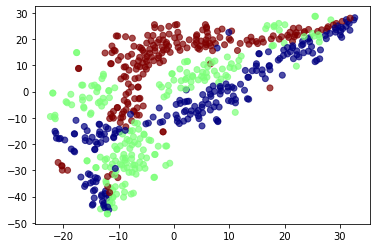
(a) DeepWalk

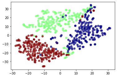
(b) GCN

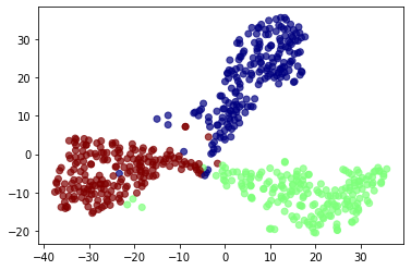
(c) TPM

Figure 5: Visualization of 2D representations for LFR network.

3.7 Cross-networks generalization: Scale-free networks

Scale-free networks have a unique position since they constitute most real-world networks [43]. They exhibit power-law degree distributions due to their heavy-tailed character. As shown in the degree-distribution graphic there are a limited number of nodes called hubs with a high degree and many numbers of nodes with a low degree. Most of the real-world networks show similar behavior and have scale-free degree distribution. For example, in social networks, there are a few users with many followers and many users with an average number of followers. Similarly, in airport networks, there are a few numbers of hub airports that have flights (have connections) to many different airports and many small airports which have flights to limited other airports. Therefore it is important to work and test the proposed algorithm, TPM, for scale-free networks.

Therefore, we perform the task of cross-networks generalization, which is learning information from networks of similar connectivity structures to make predictions on new networks. In this experiment, we conduct a link prediction task on networks previously unseen during training. We generate 12 Barabási-Albert networks (BA) with the following parameters: $n=\{1000,10000\}$ (number of nodes) and $\alpha=6$ (how many existing nodes may be attached to a new one). We train each embedding method on ten networks and then calculate the average AUC score on two test networks. We compare the performance of our proposed TPM model with four feature extraction algorithms (DeepWalk, node2vec, GCN, and GraphSAGE), and the experimental results are shown in Table 6. For all random walk-based models (TPM, DeepWalk, and node2vec), we run a total of $50$ random walks of $10$ steps for each node (5 random walks from each generated training Barabási-Albert network). For all graph convolutional networks-based models (GCN and GraphSAGE), we perform information aggregation per node evenly from ten generated training Barabási-Albert networks. Moreover, in the generated Barabási-Albert networks, nodes lack features. For features, we use node degrees and an embedding weight that is updated for each node during training. Table 6 shows that TPM significantly outperforms all four feature extraction algorithms. These results demonstrate that our TPM model well captures the local structural patterns of nodes, even in different networks having similar topologies.

Table 6: Summary of results in terms of cross-networks generalization for two scale-free networks. Bold values mean the best results.

	DeepWalk	node2vec	GCN	GSAGE	TPM
Scale-free networks ($n=1,000$)	0.611	0.664	0.702	0.713	0.746
Scale-free networks ($n=10,000$)	0.620	0.659	0.719	0.717	0.751

3.8 Parameter Sensitivity

The proposed embedding algorithm, TPM, includes two essential hyper-parameters, $\eta$, and $m$, the number of walks per node and the length of walks. The Micro-F1 score of node classification over Cora, Citeseer, and Pubmed with various $\eta$ and $m$ demonstrate the impact of the hyper-parameters in TPM. The number of walks per node $\eta$ and length of walks $m$ were set to $\{5,10,15,20,25,30\}$ and $\{5,8,10,15,20,30,50\}$. The training ratio was set to $80\%$, and the results can be seen in Figure 6. As shown in Figure 6(a), the performance of the proposed model is relatively steady over the three citation networks when $\eta$ varies from $20$ to $30$. Hence, the larger the number of walks, the better the model’s performance since the characteristic connectivity structure of the region around the given node is captured more thoroughly. In Figure 6(b), the proposed embedding algorithm TPM achieves the best Micro-F1 score over the three citation networks when $m$ equals $10$. The score gradually decreases with increasing walk length because the walker may move away from the node’s neighborhood when the walk length $m$ is too large, thereby failing to incorporate local structural patterns properly into the walk statistics. Consequently, the parameters $\eta$ and $m$ must be tuned appropriately for various applications.

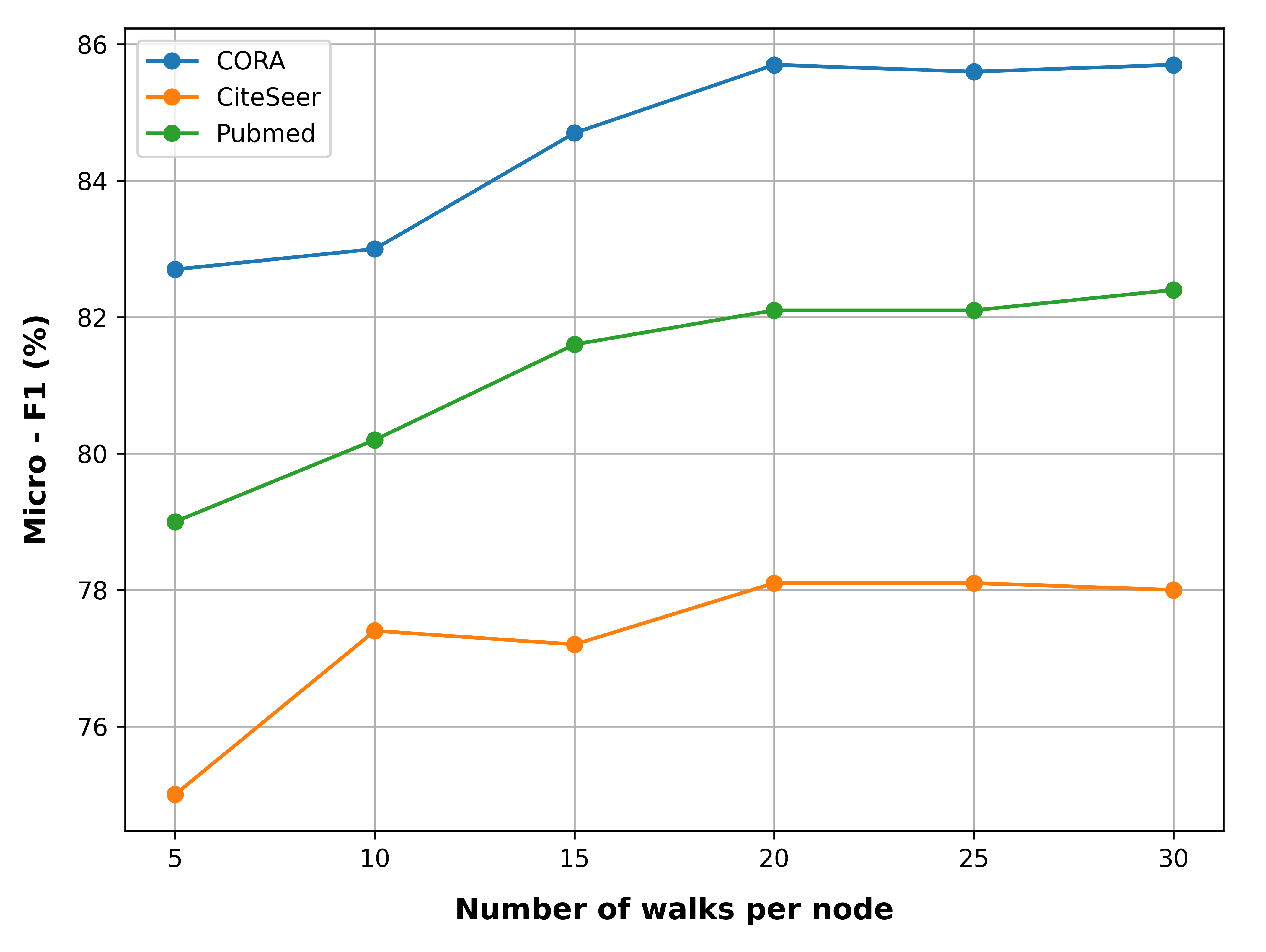
(a)

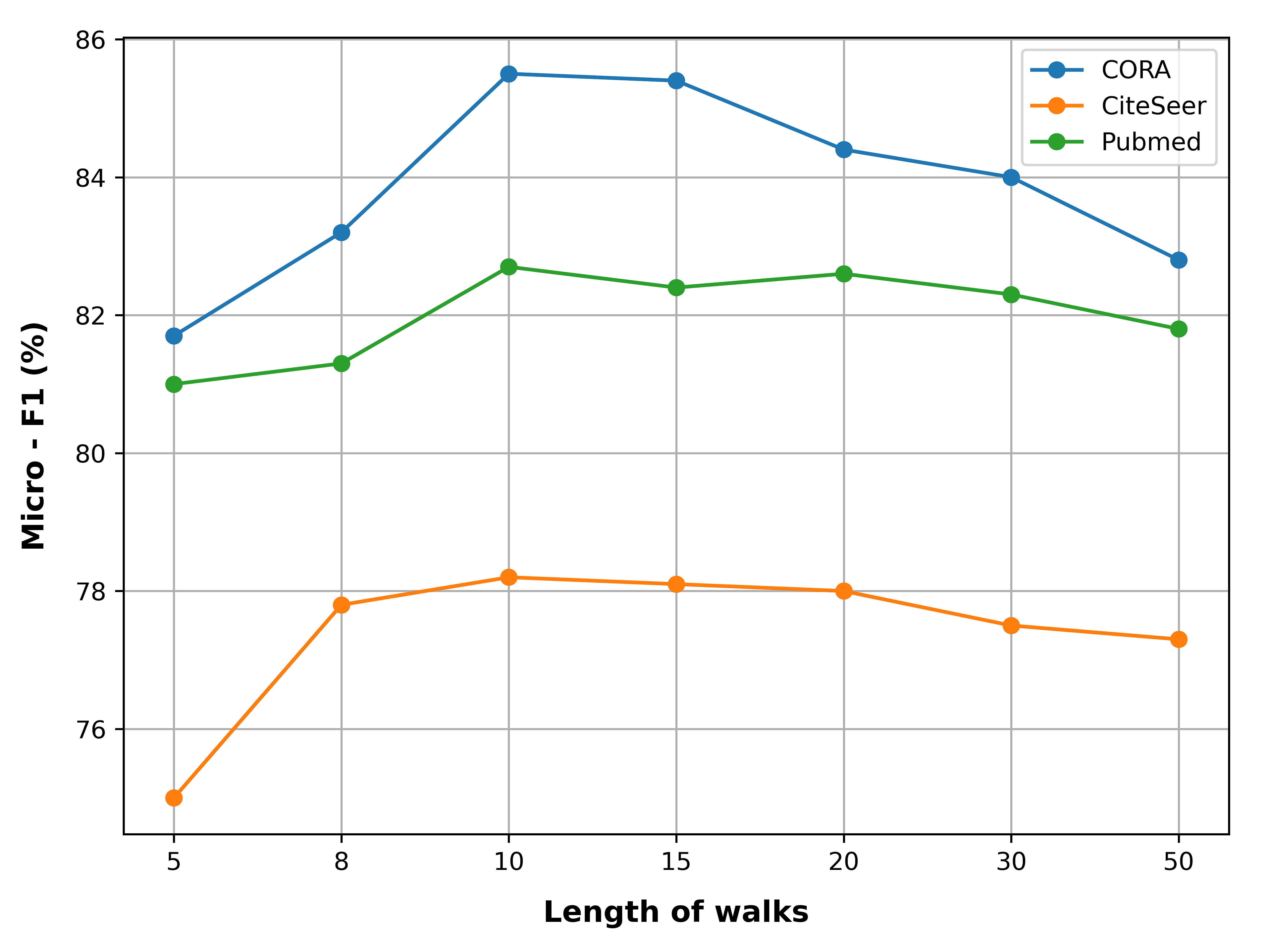
(b)

Figure 6: Results of parameter experiment. ($a$) Effect of the number of walks $\eta$ on three citation networks. ($b$) Effect of the length of walks $m$ on three citation networks.

4 Conclusions

The traditional machine learning frameworks can only be applied to networks, by mapping high-dimensional information contained in the network, to low-dimensional vector spaces. Hence, a vector representation of each node, called node embedding, is an essential initial step for processing the data obtained from networks. The embedding algorithm must represent the graph’s connectivity structure, which requires mixing properties of nodes and edges. Most of the existing representation learning techniques concentrate only on the local structure of nodes, hence lacking representation of local structural patterns in downstream network analysis tasks.

The present study introduces a new, scalable unsupervised node embedding algorithm that inherently contains the local connectivity structure of the nodes. Moreover, node similarities are also part of the embedding representation since the node embeddings overlap. The proposed algorithm uses anonymous walks for structural node embeddings. Starting from a given node, each walk collects local structural information in a predetermined neighborhood radius. A unique transition probability matrix represents each node in the network. Elements of each transition probability matrix consist of the probability of reaching the neighboring nodes starting from the original. Hence the transition probability matrices of neighboring nodes overlap. The overlapping transition probability matrices ensure the correct similarity measures between the neighboring nodes. The significant advantage of the proposed method is to capture local structural patterns rather than the identity of a node by visiting a limited number of close neighbors using short random walks. This reduces computation time, improves performance, and gathers information without going deep into a graph. Moreover, the transition probability matrix method has superior prediction potential in identifying similar connectivity structures in remote network parts. This possibility extends the use of the proposed embedding vectors, created using the information of a given network, onto unstudied networks. The flattened transition probability matrix elements are used as node feature vectors in the present work. Experiments on three commonly used real-world networks and synthetic networks, presented in the experiments section, demonstrated the effectiveness of the proposed method (TPM). For future work, the extensibility of TPM on attributed networks and temporal dynamic networks will be considered.

References

- [1] Réka Albert and Albert-László Barabási. Statistical mechanics of complex networks. Reviews of Modern Physics, 74(1):47, 2002.
- [2] Albert-László Barabási. Network science. Philosophical Transactions of the Royal Society A: Mathematical, Physical and Engineering Sciences, 371(1987):20120375, 2013.
- [3] Xiaohui Han, Lianhai Wang, Chaoran Cui, Jun Ma, and Shuhui Zhang. Linking multiple online identities in criminal investigations: A spectral co-clustering framework. IEEE Transactions on Information Forensics and Security, 12(9):2242–2255, 2017.
- [4] Hocine Cherifi, Gergely Palla, Boleslaw K Szymanski, and Xiaoyan Lu. On community structure in complex networks: challenges and opportunities. Applied Network Science, 4(1):1–35, 2019.
- [5] Kuo Chi, Guisheng Yin, Yuxin Dong, and Hongbin Dong. Link prediction in dynamic networks based on the attraction force between nodes. Knowledge-Based Systems, 181:104792, 2019.
- [6] Santo Fortunato. Community detection in graphs. Physics Reports, 486(3-5):75–174, 2010.
- [7] Pelin Cetin and Sahin Emrah Amrahov. A new overlapping community detection algorithm based on similarity of neighbors in complex networks. Kybernetika, 58(2):277–300, 2022.
- [8] Smriti Bhagat, Graham Cormode, and S Muthukrishnan. Node classification in social networks. In Social Network Data Analytics, pages 115–148. Springer, 2011.
- [9] Víctor Martínez, Fernando Berzal, and Juan-Carlos Cubero. A survey of link prediction in complex networks. ACM Computing Surveys (CSUR), 49(4):1–33, 2016.
- [10] Gueorgi Kossinets and Duncan J Watts. Empirical analysis of an evolving social network. science, 311(5757):88–90, 2006.
- [11] Roberto Tamassia. Handbook of graph drawing and visualization. CRC press, 2013.
- [12] Ke Sun, Lei Wang, Bo Xu, Wenhong Zhao, Shyh Wei Teng, and Feng Xia. Network representation learning: From traditional feature learning to deep learning. IEEE Access, 8:205600–205617, 2020.
- [13] Xiao-Meng Zhang, Li Liang, Lin Liu, and Ming-Jing Tang. Graph neural networks and their current applications in bioinformatics. Frontiers in genetics, 12, 2021.
- [14] Angelo Mele. A structural model of homophily and clustering in social networks. Journal of Business Economic Statistics, pages 1–13, 2021.
- [15] Ondřej Vencálek and Daniel Hlubinka. A depth-based modification of the k-nearest neighbour method. Kybernetika, 57(1):15–37, 2021.
- [16] Peter W Battaglia, Jessica B Hamrick, Victor Bapst, Alvaro Sanchez-Gonzalez, Vinicius Zambaldi, Mateusz Malinowski, Andrea Tacchetti, David Raposo, Adam Santoro, Ryan Faulkner, et al. Relational inductive biases, deep learning, and graph networks. arXiv preprint arXiv:1806.01261, 2018.
- [17] Ziwei Zhang, Peng Cui, and Wenwu Zhu. Deep learning on graphs: A survey. IEEE Transactions on Knowledge and Data Engineering, 2020.
- [18] David Liben-Nowell and Jon Kleinberg. The link-prediction problem for social networks. Journal of the American Society for Information Science and Technology, 58(7):1019–1031, 2007.
- [19] Maria Evangelia G Pavlopoulou, Grigorios Tzortzis, Dimitrios Vogiatzis, and George Paliouras. Predicting the evolution of communities in social networks using structural and temporal features. In 2017 12th International Workshop on Semantic and Social Media Adaptation and Personalization (SMAP), pages 40–45. IEEE, 2017.
- [20] Taleb Khafaei, Alireza Tavakoli Taraghi, Mehdi Hosseinzadeh, and Ali Rezaee. Tracing temporal communities and event prediction in dynamic social networks. Social Network Analysis and Mining, 9(1):1–11, 2019.
- [21] Gergely Palla, Imre Derényi, Illés Farkas, and Tamás Vicsek. Uncovering the overlapping community structure of complex networks in nature and society. nature, 435(7043):814–818, 2005.
- [22] Mengjia Xu. Understanding graph embedding methods and their applications. SIAM Review, 63(4):825–853, 2021.
- [23] Bryan Perozzi, Rami Al-Rfou, and Steven Skiena. Deepwalk: Online learning of social representations. In Proceedings of the 20th ACM SIGKDD International Conference on Knowledge Discovery and Data Mining, pages 701–710, 2014.
- [24] Aditya Grover and Jure Leskovec. node2vec: Scalable feature learning for networks. In Proceedings of the 22nd ACM SIGKDD International Conference on Knowledge Discovery and Data Mining, pages 855–864, 2016.
- [25] Sergey Ivanov and Evgeny Burnaev. Anonymous walk embeddings. In International Conference on Machine Learning, pages 2186–2195. PMLR, 2018.
- [26] Silvio Micali and Zeyuan Allen Zhu. Reconstructing markov processes from independent and anonymous experiments. Discrete Applied Mathematics, 200:108–122, 2016.
- [27] Pelin Cetin and Şahin Emrah Amrahov. A new network-based community detection algorithm for disjoint communities. Turkish Journal of Electrical Engineering and Computer Sciences, 30(6):2190–2205, 2022.
- [28] Andrew Kachites McCallum, Kamal Nigam, Jason Rennie, and Kristie Seymore. Automating the construction of internet portals with machine learning. Information Retrieval, 3(2):127–163, 2000.
- [29] C Lee Giles, Kurt D Bollacker, and Steve Lawrence. Citeseer: An automatic citation indexing system. In Proceedings of the Third ACM Conference on Digital Libraries, pages 89–98, 1998.
- [30] Prithviraj Sen, Galileo Namata, Mustafa Bilgic, Lise Getoor, Brian Galligher, and Tina Eliassi-Rad. Collective classification in network data. AI magazine, 29(3):93–93, 2008.
- [31] Bonaventure Molokwu, Shaon Bhatta Shuvo, Narayan C Kar, and Ziad Kobti. Node classification and link prediction in social graphs using rlvecn. In 32nd International Conference on Scientific and Statistical Database Management, pages 1–10, 2020.
- [32] Yu Xie, Peixuan Jin, Maoguo Gong, Chen Zhang, and Bin Yu. Multi-task network representation learning. Frontiers in Neuroscience, 14:1, 2020.
- [33] Sarmad N Mohammed and Semra Gündüç. Degree-based random walk approach for graph embedding. Turkish Journal of Electrical Engineering and Computer Sciences, 30(5):1868–1881, 2022.
- [34] Davide Buffelli and Fabio Vandin. The impact of global structural information in graph neural networks applications. Data, 7(1):10, 2022.
- [35] Jian Tang, Meng Qu, Mingzhe Wang, Ming Zhang, Jun Yan, and Qiaozhu Mei. Line: Large-scale information network embedding. In Proceedings of the 24th International Conference on World Wide Web, pages 1067–1077, 2015.
- [36] Max Welling and Thomas N Kipf. Semi-supervised classification with graph convolutional networks. In J. International Conference on Learning Representations (ICLR 2017), 2016.
- [37] Will Hamilton, Zhitao Ying, and Jure Leskovec. Inductive representation learning on large graphs. Advances in neural information processing systems, 30, 2017.
- [38] Petar Velickovic, Guillem Cucurull, Arantxa Casanova, Adriana Romero, Pietro Lio, and Yoshua Bengio. Graph attention networks. stat, 1050:20, 2017.
- [39] Mohammed J Zaki, Wagner Meira Jr, and Wagner Meira. Data mining and analysis: fundamental concepts and algorithms. Cambridge University Press, 2014.
- [40] James A Hanley and Barbara J McNeil. The meaning and use of the area under a receiver operating characteristic (roc) curve. Radiology, 143(1):29–36, 1982.
- [41] Michelle Girvan and Mark EJ Newman. Community structure in social and biological networks. Proceedings of the National Academy of Sciences, 99(12):7821–7826, 2002.
- [42] Andrea Lancichinetti, Santo Fortunato, and Filippo Radicchi. Benchmark graphs for testing community detection algorithms. Physical Review E, 78(4):046110, 2008.
- [43] Albert-László Barabási and Eric Bonabeau. Scale-free networks. Scientific American, 288(5):60–69, 2003.