Granger Causality using Neural Networks

Abstract

The Granger Causality (GC) test is a famous statistical hypothesis test for investigating if the past of one time series affects the future of the other. It helps in answering the question whether one time series is helpful in forecasting -another (Granger, 1969). Standard traditional approaches to Granger causality detection commonly assume linear dynamics, but such simplification does not hold in many real-world applications, e.g., neuroscience or genomics that are inherently non-linear. In such cases, imposing linear models such as Vector Autoregressive (VAR) models can lead to inconsistent estimation of true Granger Causal interactions. Machine Learning (ML) can learn the hidden patterns in the datasets specifically Deep Learning (DL) has shown tremendous promise in learning the non-linear dynamics of complex systems. Recent work of Tank et al. (2018) propose to overcome the issue of linear simplification in VAR models by using neural networks combined with sparsity-inducing penalties on the learn-able weights. The authors propose a class of non-linear methods by applying structured multilayer perceptrons (MLPs) or recurrent neural networks (RNNs) for prediction of each time series separately using Component Wise MLPs and RNNs. Sparsity is achieved through the use of convex group-lasso penalties. The sparsity penalties encourage specific sets of weights to be zero (or very small), allowing the Granger Causal structure to be extracted.

In this work, we build upon ideas introduced by Tank et al. (2018). We propose several new classes of models that can handle underlying non-linearity. Firstly, we present the Learned Kernal VAR(LeKVAR) model—an extension of VAR models that also learns kernel parametrized by a neural net. Secondly, we show one can directly decouple lags and individual time series importance via decoupled penalties. This decoupling provides better scaling and allows us to embed lag selection into RNNs. Lastly, we propose a new training algorithm that supports mini-batching, and it is compatible with commonly used adaptive optimizers such as Adam (Kingma and Ba, 2014). The proposed techniques are evaluated on several simulated datasets inspired by real-world applications.We also apply these methods to the Electro-Encephalogram (EEG) data for an epilepsy patient to study the evolution of GC before , during and after seizure across the 19 EEG channels.

,

, and

1 Introduction

In many scientific applications related to multivariate time series, it is important to predict or forecast and understand the underlying structure within time series. Often, we are interested in the interactions between and within individual time series, and our goal is to infer information about the current and lagged relationships between and across series. Typical examples include neuroscience, where it is important to determine how brain activation spreads through brain regions (Sporns, 2010; Vicente et al., 2011; Stokes and Purdon, 2017; Sheikhattar et al., 2018); or finance, where it is important to determine groups of stocks with low covariance to design low risk portfolios (Sharpe, Alexander and Bailey, 1968); and biology, where it is of great interest to infer gene regulatory networks from time series of gene expression levels (Fujita et al., 2010; Lozano et al., 2009a). Such goal requires models that can extract these structural dependencies in the highly non-linear dynamics.

1.1 Granger Causality

Among the many choices for understanding relationships between time series, Granger causality (Granger, 1969; Lütkepohl, 2005) is a commonly used framework for time series structure discovery that quantifies whether the past of one time series helps in predicting the future values of another time series. Granger defined the causality relationship based on two principles:

1. The cause happens prior to its effect.

2. The cause has unique information about the future values of its effect.

Given these two assumptions about causality, Granger proposed to test the following hypothesis for identification of a causal effect of $X$ on $Y$

$$\exists\;t\in\{1,2,\ldots T\}\text{ s.t. }\mathbb{P}[Y(t+1)\in A\mid{\mathcal{I}}(t)]\neq\mathbb{P}[Y(t+1)\in A\mid{\mathcal{I}}_{-X}(t)],$$ (1)

where $\mathbb{P}$ refers to probability, $A$ is an arbitrary non-empty set, and $\mathcal{I}(t)$ and $\mathcal{I}_{-X}(t)$ respectively denote the information available as of time $t$ in the entire universe, and that in the modified universe in which $X$ is excluded. If the above hypothesis is accepted, we say that $X$ Granger-Causes $Y$.

GC also allows the study of an entire system of time series to uncover networks of causal interactions (Basu, Shojaie and Michailidis, 2015). Other types of structure discovery, like coherence (Sameshima and Baccala, 2016) or lagged correlation (Sameshima and Baccala, 2016) do not have such benefit as they analyze strictly bivariate relationships which limits their use in inferring high dimensionality. This property makes GC a valuable tool to analyze high-dimensional complex data streams.

The methodology for testing GC may be separated into model-based and model-free classes.

1.1.1 Model-based Approach

The majority of model-based methods assume linear dependence and use some form of the widely popular vector autoregressive (VAR) model (Lozano et al., 2009a; Lütkepohl, 2005). In this case, the past time lags of a series are assumed to have a linear effect on the future of the series being predicted, and the non-zero (or large enough) coefficients quantify and characterize the Granger causal effect. Sparsity-inducing regularizers, like the Lasso (Tibshirani, 1996) or group lasso (Yuan and Lin, 2006), help scale linear GC estimation in VAR models to the high-dimensional setting (Lozano et al., 2009a; Basu et al., 2015). For the overview of optimization with sparsity-induced penalties, we refer the reader to (Bach et al., 2012).

As previously discussed, assuming linear dependence can lead to misinterpretation of non-linear relationships and produce inconsistent and misleading estimates of the true underlying structure due to over simplification. To overcome this issue, Sun (2008) incorporated kernel functions to model non-linearity. However, the kernel function has to be selected manually for kernel-based methods which can be a difficult task, because the chosen kernel functions might not necessarily be suitable for representing specific non-linearity observed in data. Another possibility is to employ neural networks (NN) to handle non-linearity by learning the kernel function from the data. We dedicate a separate subsection later in this section for this approach.

1.1.2 Model-free Approach

Model-based methods may fail in real-world cases when there is a misspecification between classes of function that the model can represent and the true underlying relationships (Teräsvirta et al., 2010; Tong, 2011; Lusch, Maia and Kutz, 2016). Such a case can typically arise when the linear model is assumed, and there are non-linear dependencies between the past and the future observations. Model-free methods, including transfer entropy (Vicente et al., 2011) or directed information (Amblard and Michel, 2011) can overcome these non-linear dependencies with minimal assumptions about the underlying relationships. However, these estimators could lead to high level of uncertainty due to a significant degree of freedom, and they might require large amounts of data to obtain reasonable estimates. In addition, these approaches also suffer from a curse of dimensionality (Runge et al., 2012) when the number of time series grows, making them inappropriate in the high-dimensional setting.

1.1.3 Neural Networks and Granger Causality

Neural networks are capable of representing complex, non-linear, and non-additive interactions between inputs and outputs via a learning a series of transformations. As previously observed, their time series variants, such as Autoregressive Multilayer Perceptrons (MLPs) (Raissi, Perdikaris and Karniadakis, 2018; Kişi, 2004; Billings, 2013) and Recurrent Neural Networks (RNNs) like long-short term memory networks (LSTMs) (Hochreiter and Schmidhuber, 1997) have shown impressive performance in forecasting multivariate time series (Yu et al., 2017; Zhang, 2003; Li et al., 2017). Unfortunately, while these methods have demonstrated promising predictive performance, they are essentially black-box methods and provide little if any interpretability of the underlying structural dependencies in the series.

The challenge of interpretability was recently studied in (Tank et al., 2018), where the authors present a framework for structure learning in MLPs and RNNs that leads to interpretable non-linear GC discovery. Their framework contains three main ingredients— i) the impressive flexibility and representational power of neural networks to learn the complex structure in the data, ii) separate models per single output series, i.e., component-wise architecture that disentangles the effects of lagged inputs on individual output series, and iii) sparsity-inducing penalties on the input layer that enables interpretability. The authors propose to place sparsity-inducing penalties on particular groupings of the weights that relate the histories of individual series to the output series of interest. They term these as sparse component-wise models, e.g. cMLP and cLSTM, when applied to the MLP and LSTM, respectively. In particular, they use group sparsity penalties (Yuan and Lin, 2006) on the outgoing weights of the inputs for GC discovery or their more structured versions (Nicholson, Bien and Matteson, 2014; Huang, Zhang and Metaxas, 2011) (Kim and Xing, 2010) that automatically detect both non-linear GC and also the lags of each inferred interaction.

2 Contributions

In this work, we build on these previous works tackling Granger causality on neural networks with the following key contributions.

• We propose a novel model to learn non-linear relations by combining kernel-based methods and VAR models. In contrast to standard kernel methods, where the kernel function must be selected manually, we model it as a neural network which learns the shared kernel as a part of the training process. This construction helps to model better the specific non-linearity coming from data. We refer to this model as the Learned Kernel Vector AutoRegressive (LeKVAR) model.

• For Granger causality, we are interested to understand the importance of each time series component. The standard way to model GC using neural networks is to focus on the effect of each combination of lag and time-series component and then extract the importance of each time series component as a summation over lags. In this work, we propose a simple and elegant approach to measure the significance of each lag and time series component by decoupling the lag and the time series using an attention based approach. We include separate sparsity-inducing penalties for time series components and lags. We believe that such decoupling is less prone to over-fitting and provides a better estimate of GC. In addition, to the best of our knowledge, this novel approach is the first to enable direct lag extraction from recurrent neural models.

• We show that previous approaches including our proposed models can’t be naively applied as the learning objective happens to be degenerated. We propose a solution to overcome this issue by building the weight normalization into the learning.

• We propose a new training algorithm to detect GC that, in contrast to previous approaches, enables mini-batching, which is one of the crucial building blocks of deep learning (DL) optimizers. Our solution is to directly incorporate penalty into the loss function that also allows us to use popular adaptive optimizers such as Adam (Kingma and Ba, 2014) by avoiding the proximal step. We realize that such modification does not lead to exact zeros for GC, but we find it easy to select the threshold by examining obtained GC coefficients.

• We study the evolution of the GC between EEG channels for an epilepsy patient before, during and after the seizure using these methods.

3 Granger Causality for VAR

In this section, we firstly showcase how the GC is done for VAR models, which will be useful to further extend this idea into neural network settings. Let ${\bf x}_{t}\in\mathbb{R}^{p}$ be a $p$-dimensional stationary time series and assume we have observed the process at $T$ time points, $({\bf x}_{1},\ldots,{\bf x}_{T})$. We use the VAR model to detect Granger causality in time series analysis (Lütkepohl, 2005). In this model, the time series at time $t$, ${\bf x}_{t}$, is assumed to be a linear combination of the past $K$ lags of the series

$${\bf x}_{t}=\sum_{k=1}^{K}A^{(k)}{\bf x}_{t-k}+e_{t},$$ (2)

where $A^{(k)}$ is a $p\times p$ matrix that specifies how lag $k$ affects the future evolution of the series and $e_{t}$ is zero mean noise. In this model, time series $j$ does not Granger-cause time series $i$ if and only if for all $k$, $A_{ij}^{(k)}=0$. A Granger causal analysis in the VAR model thus reduces to determining which values in $A^{(k)}$ are zero over all lags. In higher dimensional settings, this may be determined by solving a group lasso regression problem (Lozano et al., 2009b)

$$\min_{A^{(1)},\ldots,A^{(K)}}\sum_{t=K}^{T}\|{\bf x}_{t}-\sum_{k=1}^{K}A^{(k)}{\bf x}_{t-k}\|_{2}^{2}+\lambda\sum_{ij}\|(A_{ij}^{(1)},\ldots,A^{(K)}_{ij}\|_{2},$$ (3)

where $\|\cdot\|_{2}$ denotes the standard $L_{2}$ norm. The group lasso penalty over all lags of each $(i,j)$ entry, $\|(A_{ij}^{(1)},\ldots,A^{(K)}_{ij}\|_{2}$ jointly shrinks all $A_{ij}^{k}$ parameters to zero across all lags $k$ (Yuan and Lin, 2006). The sum over all $(i,j)$ $L_{2}$ norms of $(A_{ij}^{(1)},\ldots,A_{ij}^{(K)})$ is known as a group lasso penalty, and jointly shrinks all $A_{ij}^{k}$ parameters to zero across all lags $k$ (Yuan and Lin, 2006). The hyperparameter $\lambda>0$ controls the level of group sparsity.

The group penalty in Equation (3) may be replaced with a structured hierarchical penalty (Huang, Zhang and Metaxas, 2011; Jenatton et al., 2011) that automatically selects the lag of each Granger causal interaction (Nicholson, Bien and Matteson, 2014).

The main advantage of this approach is its simplicity and straightforward extraction of GC. On the other hand, the VAR model assumes linear dependence, which might be a too strong assumption, and, therefore, the model will not be able to capture non-linear dependencies.

4 Granger Causality with Neural Networks

In this section, we firstly introduce the general non-linear approach introduced in (Billings, 2013). A non-linear autoregressive model (NAR) allows ${\bf x}_{t}\in\mathbb{R}^{p}$ to evolve according to more general non-linear dynamics

$${\bf x_{t}}=g(x_{<t1},\ldots,x_{<tp})+e_{t}$$ (4)

where $x_{<ti}=\left(\ldots,x_{(t-2)i},x_{(t-1)i}\right)$ denotes the past of series $i$ and we assume additive uncorrelated zero mean white noise $e_{t}$.

Standard approach to jointly model the full non-linear functions $g$ is to use neural networks. Neural networks have been sucessfully used in NAR forecasting (Billings, 2013; Chu, Shoureshi and Tenorio, 1990; Billings and Chen, 1996; Yu et al., 2017; Li et al., 2017; Tao et al., 2018). These approaches either utilize MLPs where the inputs are $x_{<t}=x_{(t-1):(t-K)}$, for some lag $K$, or a recurrent neural networks, like the LSTM cell.

As previously discussed, the standard plain neural networks act as black boxes which makes them difficult for interpretation, essentially useless for Granger causality. Another issue is that modelling all the times series together might lead to misleading results. Specifically, shared weights allows series $j$ to Granger-cause series $i$ but not Granger-cause series $i^{\prime}$ for $i\neq i^{\prime}$, which can’t be inferred from the model. Therefore, a joint network over all $x_{ti}$ for all $i$ implicitly assumes that each time series depends on the same past lags of the other series. However, in practice, each $x_{ti}$ may depend on different past lags of the other series.

To tackle these issues, Tank et al. (2018) proposed to use component-wise neural networks with sparsity-induce penalties that allow to extract Granger causality from input connections similarly to the VAR model.

In more formal way, the general component-wise model is of the following form

$$x_{ti}=g_{i}\left(x_{<t1},\ldots,x_{<tp}\right)+e_{ti},$$

where, $g_{i}$ is a function that specifies how the past $K$ lags are mapped to series $i$, e.g., modelled by a neural network. In this context, Granger non-causality between two series $j$ and $i$ means that the function $g_{i}$ does not depend on $x_{<tj}$, the past lags of series $j$. Such statement can be formalized as

Definition 4.1.

Time series $j$ is Granger non-causal for time series $i$ if for all $\left(x_{<t1},\ldots,x_{<tp}\right)$ and all $x^{\prime}_{<tj}\neq x_{<tj}$,

$$g_{i}\left(x_{<t1},\ldots,x_{<tj},\ldots,x_{<tp}\right)=g_{i}\left(x_{<t1},\ldots,x^{\prime}_{<tj},\ldots x_{<tp}\right)$$

that is, $g_{i}$ is invariant to $x_{<tj}$.

As previously mentioned, one possibility is to model $g_{i}$ as a neural network model. Let us define $W^{(i,j)}_{k}$ to be a set of weights of the first layer of $g_{i}$ that connects to the time series $j$ at lag $k$. Note here that for RNNs $W^{(i,j)}_{k}$ is the same as $W^{(i,)_{k^{\prime}}}$ for all $k,k^{\prime}$. The above definition is then satisfied if all weights that belong to $W^{(i,j)_{k}}$ are zeros. To make this condition sufficient and necessary, one needs to introduce a regularization term. We denote this penalty with $\Omega\left(W^{(i,j)}\right)$, where is union accross all the lags, i.e.,

$$W^{(i,j)}=\cup_{k=1}^{K}W^{(i,j)_{k}}.$$

We scale this penalty with coefficient $\lambda$ that determines sparsity level.

Some of the popular choices are listed below.

• A group lasso penalty over the entire set of outgoing weights across all lags for time series $j$, $W^{(i,j)}$,

  $$\Omega\left(W^{(i,j)}\right)=\left\|\text{vec}(W^{(i,j)})\right\|_{2},$$ (5)

  where $\text{vec}(\cdot)$ transforms set of weights into a vector. This penalty shrinks all weights associated with lags for input series $j$ equally. For large enough $\lambda$, the solutions will lead to many zero columns in each set $W^{(i,j)}$, implying only a small number of estimated Granger causal connections. This group penalty is the neural network analogue of the group lasso penalty across lags in equation (3) for the VAR case.

• To detect also the lags where Granger causal effects exists, it was proposed in the literature (Tank et al., 2018) to add group lasso penalty across each lag. This penalty assumes that only a few lags of a series $j$ are predictive of series $i$ and provides both sparsity across groups (a sparse set of Granger causal time series) and sparsity within groups (a subset of relevant lags)

  $$\Omega\left(W^{(i,j)}\right)=\alpha\left\|\text{vec}(W^{(i,j)})\right\|_{2}+(1-\alpha)\sum_{k=1}^{K}\left\|\text{vec}(W^{(i,j)}_{k})\right\|_{2}$$ (6)

  where $\alpha\in(0,1)$ controls the trade-off in sparsity across and within groups. This penalty is a related to, and is a generalization of, the sparse group lasso (Simon et al., 2013).

• One can also put more penalty to larger lags to simultaneously select for both Granger causality and the lag order of the interaction by replacing the group lasso penalty with a hierarchical group lasso penalty (Nicholson, Bien and Matteson, 2014),

  $$\Omega\left(W^{(i,j)}\right)=\sum_{k=1}^{K}\left\|\left(\text{vec}(W^{(i,j)}_{k}),\ldots,\text{vec}(W^{(i,j)}_{K})\right)\right\|_{2}.$$ (7)

  By construction, the hierarchical penalty promotes the solutions such that for each $j$ there exists a lag $k$ such that all the elements of $W^{(i,j)}_{k^{\prime}}$ all zeros for $k^{\prime}>k$ and some elements of $W^{(i,j)}_{k^{\prime}}$ are non-zero for $k^{\prime}\leq k$. Thus, this penalty effectively selects the lag of each interaction. The hierarchical penalty also pushes many columns of $W^{(i,j)}_{k}$ to be zero across all $k$, effectively selecting for Granger causality. In practice, the hierarchical penalty allows us to fix $K$ to a larger value, ensuring that no Granger causal connections at higher lags are missed. Lastly, note that this penalty is not naively applicable to RNNs.

5 LeKVAR

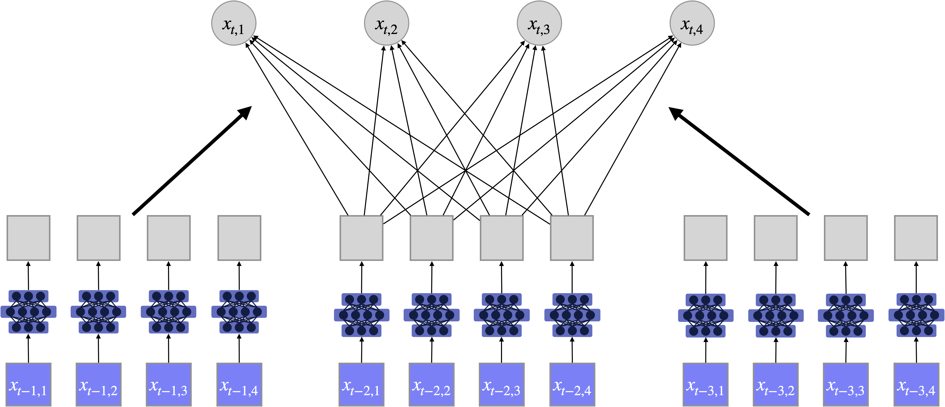
Figure 1: A schematic for the non-linear LeKVAR. The input is first transformed using a shared learned kernel displayed as a small purple neural network. Then each transformed input is linearly combined to form the final output. The round output neurons ($x_{t,i}$) represent summation operation of incoming connections. We say that the series $j$ does not Granger-cause series $i$ if outgoing weights for series $j$, shown as dark arrows connecting gray squares with the output, are zeros. We say that the lag $k$ does not Granger-cause series $i$ if outgoing weights for series $[x_{t-k,1},x_{t-k,2},\ldots,x_{t-j,p}]$, shown as dark arrows connecting gray squares with the output, are zeros.

This section proposes an extension of the GC VAR model that incorporates the learned kernel into the training process. We follow the same notation as introduced in Section 3. In our new model, the time series at time $t$, ${\bf x}_{t}$, is assumed to be a linear combination of the past $K$ lags of the series transformed by a shared kernel

$${\bf x}_{t}=\sum_{k=1}^{K}A^{(k)}\xi({\bf x}_{t-k})+e_{t},$$ (8)

where $\xi(\cdot)$ is the element-wise kernel function $\mathbb{R}\rightarrow\mathbb{R}$ parametrised by a neural network. By enforcing kernel function to act independently on each element, we preserve the desired feature of VAR models that time series $j$ does not Granger-cause time series $i$ if and only if for all $k$, $A_{ij}^{(k)}=0$ (note that in this case $W^{(i,j)}_{k}$ consists of the elements of $A_{ij}^{(k)}$). Incorporating $\xi(\cdot)$ into the training process enables learning kernel instead of manual selection. The schematic graph of the LeKVAR model is displayed in Figure 1. The limitation of the proposed model is its expressibility as we assume that there exists a shared element-wise transformation of the time series that leads to linear dependence between current and lagged values. On the other hand, shared kernel functions have access to more data as the same kernel is shared across the all component which allows for a more precise estimate and intuitively better performance when compared to a separate model for each time series component.

6 Decoupling Lags and Time Series Components

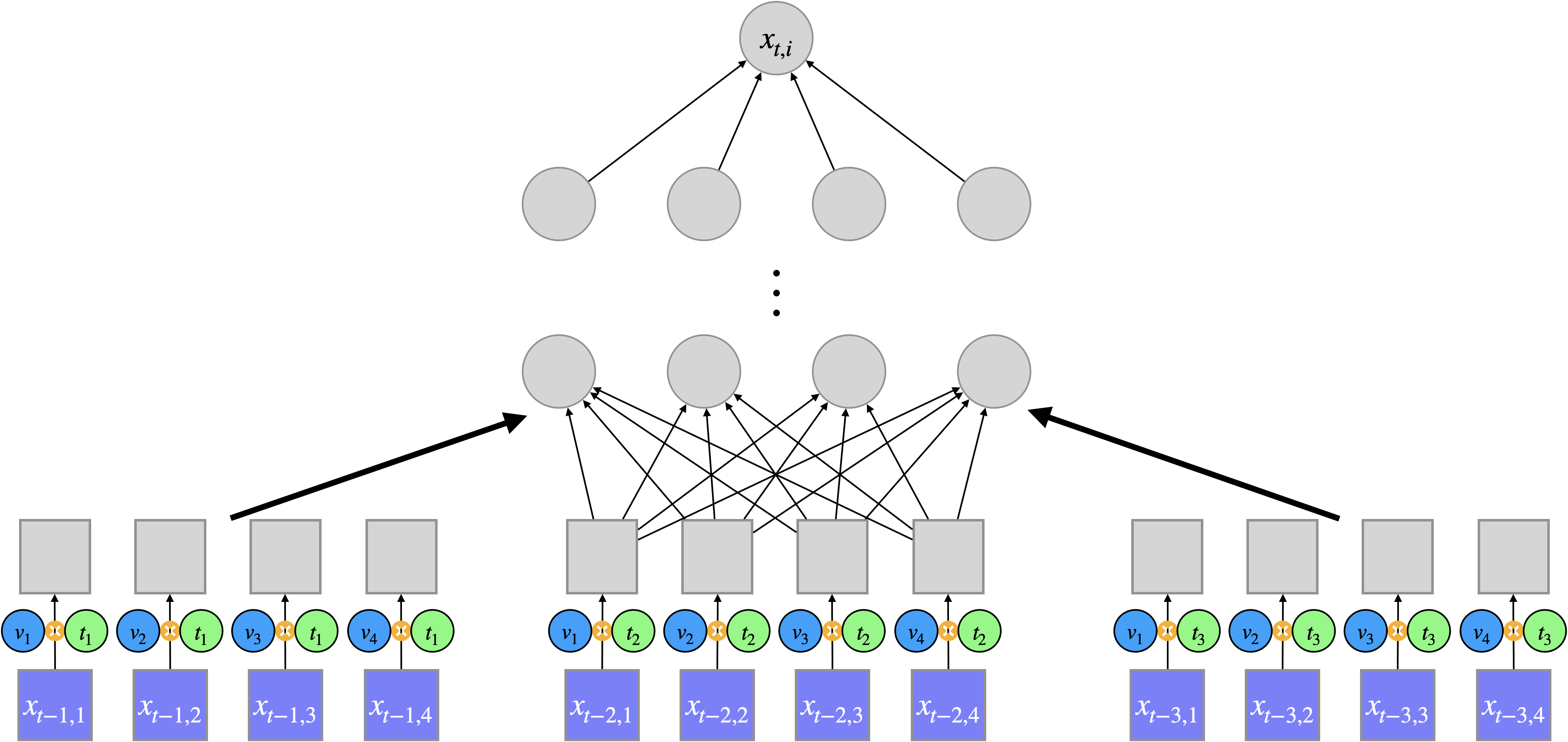
Figure 2: A schematic for the decoupling of the lags and times series components to decide Granger causality. Each input element is first multiplied by its corresponding lag and component penalty, i.e., $x_{t-k,j}$ is multiplied by the product $v_{j}q_{k}$, displayed as a small purple neural network. Then the output is obtained as the output of the component-wise neural network model with the scaled input. We say that the series $j$ does not Granger-cause series $i$ if the corresponding $v_{j}$ for the component-wise neural network to predict $x_{t,i}$, shown as a blue circle, is zero. We say that the lag $k$ does not Granger-cause series $i$ if the corresponding $q_{k}$ for the component-wise neural network to predict $x_{t,i}$, shown as a green circle, is zero.

Granger causality’s main objective is to decide whether time series $j$ does not Granger-cause time series $i$. As we saw in the previous sections, a typical approach to decide on Granger-cause of time series $j$ to time series $i$ is to look at the weights $W^{(i,j)}$ and compute its square norm. If this is less than some predefined threshold, we say time series $j$ does not Granger-cause time series $i$. For our new approach, we define vector $v\in\mathbb{R}^{p}$

$$v^{i}=(v^{i}_{1},v^{i}_{2},\ldots,v^{i}_{p})^{\top}$$

to correspond to the importance of each time series and $q\in\mathbb{R}^{p}$

$$q^{i}=(q^{i}_{1},q^{i}_{2},\ldots,q^{i}_{K})^{\top}$$

to conform to the extent of each time lag. To build this into the neural network model, we multiply each element of $W^{(i,j)}$ by $v^{i}_{j}$, each element $W^{(i,j)}_{k}$ by $q^{i}_{k}$ and we apply the sparsity-inducing penalties on $v^{i}$’s and $q^{i}$’s; see the schematic graph of the regularization model displayed in Figure 2. These multiplications can be implemented efficiently for standard machine learning libraries such as PyTorch. Furthermore, we note that our approach can be naively combined with any previously discussed penalty. To decide whether time series $j$ does not Granger-cause time series $i$, we look at the magnitude of $v^{i}_{j}$. This procedure decouples the neural network model and Granger causality and provides better scaling regarding the number of parameters that needs to estimated to infer GC connections. Therefore, it is natural to expect that this approach will lead to more stable and reliable estimates of GC.

Finally, our approach allows us to capture the importance of each lag, and it is model agnostic. Hence, we can apply this to recurrent neural network (RNN) blocks that have not been possible before due to shared weights across different time steps. Furthermore, our proposed framework can estimate any dependence structure and build in prior knowledge by imposing structure in $v^{i}$’s or $q_{i}$’s without the necessity to tailor GC estimates to particular models.

7 Degenerated Objective

We identify that the previous approaches to neural Granger causality including our proposed models (LeKVAR and decoupling) can’t be naively applied as the learning objective happens to be degenerated. The issue is that we might multiply two parameters, where one of them is part the sparsity-inducing penalty and the other one is not, with each other without only scaling invariant transformation in between (e.g., no transformation or ReLU activation), which can lead to undesired behaviour. Let us demonstrate the problem via the following example. We are interested in minimizing the following objective

$$\frac{1}{n}\sum_{i=1}^{n}\|v_{1}w_{1}^{\top}x^{i}_{1}+v_{2}w_{2}^{\top}x^{i}_{2}-y^{i}\|_{2}^{2}+\lambda(|v_{1}|+|v_{2}|)$$ (9)

parametrized by scalars $v_{1},v_{2}$ and vectors $w_{1},w_{2}$, where $\lambda>0$, $\{x^{i}_{1},x^{i}_{2}\}_{i=1}^{n}$ are given vectors and $\{y^{i}\}_{i=1}^{n}$ are given scalars. We note that for such objective penalty can be ignored as for any non-zero scalar $c<1$ $v^{\prime}_{1}=cv_{1}$, $v^{\prime}_{2}=cv_{2}$ and $w^{\prime}_{1}=\nicefrac{{1}}{{c}}\;w_{1}$, $w^{\prime}_{2}=\nicefrac{{1}}{{c}}\;w_{2}$ lead to the same value of the first term while decreasing the second term. Therefore, we propose following reparametrization that allows us to incorporate penalty such that it has an actual effect on sparsity of the model.

$$\frac{1}{n}\sum_{i=1}^{n}\left\|v_{1}\frac{w_{1}^{\top}x^{i}_{1}}{\|w_{1}\|_{2}}+v_{2}\frac{w_{2}^{\top}x^{i}_{2}}{\|w_{2}\|_{2}}-y^{i}\right\|_{2}^{2}+\lambda(|v_{1}|+|v_{2}|).$$ (10)

This reparametrization proceeds by normalizing weights connected to the penalty term, and it is an essential building block of our proposed methods. One can think that such reparametrization might make optimizing the objective harder. Still, as investigated in (Salimans and Kingma, 2016), normalizing weights of the network can lead to better-conditioned problems and, hence, faster convergence. Note that in case ReLU is used as the activation function the weight normalization has to be applied for each layer.

8 Optimizing the Penalized Objectives

A previously common approach to optimize the penalized objective was to run proximal gradient descent (Parikh et al., 2014). Proximal optimization was considered necessary in the context of GC because it leads to exact zeros. We propose a different training algorithm that embeds the sparsity-inducing penalty directly into the loss function and follows the standard training loop commonly considered in deep learning optimization. As such, it enables a wide variety of optimization tricks such as mini-batching, different forms of layer and weight normalizations and usage of the popular adaptive optimizers, including Adam (Kingma and Ba, 2014), which are not natively compatible with proximal steps. We realize that such modification does not lead to exact zeros for GC anymore. Still, in our experience, incorporating standard optimization tricks outweigh the issue of no exact zeros. We found it relatively easy to select the threshold by examining obtained GC coefficients in our experiments.

9 Experiments

Table 1: Comparison of AUROC and AUPR for Granger causality selection among 10 dimensional VAR(3) model, parametrised as a function of the length of the time series $T$. Results are the mean across three initializations, with one standard deviation.

	AUROC			AUPR
T	100	200	1000	100	200	1000
VAR	77.6 ± 1.2	98.9 ± 0.1	100.0 ± 0.0	49.4 ± 3.7	95.0 ± 0.0	100.0 ± 0.0
LeKVAR	65.1 ± 9.0	99.5 ± 0.4	100.0 ± 0.0	56.6 ± 6.8	98.2 ± 1.4	100.0 ± 0.0
cMLP	73.1 ± 5.4	97.5 ± 1.8	100.0 ± 0.0	53.7 ± 8.6	90.2 ± 7.0	100.0 ± 0.0
cMLPwF	69.5 ± 2.8	97.5 ± 1.3	100.0 ± 0.0	43.3 ± 8.8	91.4 ± 4.3	100.0 ± 0.0
cLSTM	74.9 ± 2.9	97.9 ± 0.8	100.0 ± 0.0	53.8 ± 5.2	94.2 ± 1.8	100.0 ± 0.0
cLSTMwF	73.6 ± 2.7	99.6 ± 0.4	100.0 ± 0.0	41.1 ± 6.1	98.9 ± 0.8	100.0 ± 0.0
cMLP_s	79.2 ± 1.9	98.6 ± 0.5	100.0 ± 0.0	60.4 ± 4.6	93.7 ± 2.0	100.0 ± 0.0
cMLPwF_s	76.3 ± 3.5	97.5 ± 1.0	100.0 ± 0.0	51.3 ± 7.0	88.6 ± 5.0	100.0 ± 0.0
cLSTM_s	78.2 ± 2.2	98.6 ± 0.5	100.0 ± 0.0	62.0 ± 5.8	94.8 ± 2.6	100.0 ± 0.0
cLSTMwF_s	74.1 ± 0.6	98.1 ± 1.0	100.0 ± 0.0	60.1 ± 2.2	94.6 ± 2.2	100.0 ± 0.0

Our implementation is publicly available and all the experiments can be reproduced using our code repository on GitHub.

We consider three tasks, namely the VAR model, Lorenz-96 Model and Dream challenge (Prill et al., 2010). We also apply our methods to EEG data for an epilepsy patient to study the evolution of GC. We provide the detailed description of each task in the corresponding section.

We compare ten models—VAR; LeKVAR introduced in Section 5, component-wise MLP (cMLP) and LSTM (cLSTM) (Tank et al., 2018) together with cLSTMwF and cMLPwF, which are the same models as original cLSTM and cMLP, respectively, with the decoupled penalty introduced in Section 6. The neural kernel of the LekVAR model is fully connected neural network with one hidden layer with 10 neurons. For cMLP(wF) and cLSTM(wF), we have two hidden layers / LSTM blocks with 10 neurons in each layer. We also include small version of these models (denoted “_s”) which have only hidden layer / LSTM block. We use sigmoid as the activation function. For EEG data we apply cMLPwF to study the GC evolution across time.

We report the area under the receiver operating characteristic (ROC) and precision-recall (PR) curves for the model with the best validation loss averaged across three independent initializations. We split each dataset randomly to the train and validation set, where the validation set consists of $20\%$ samples. For each method, we run $200$ epochs with Adam optimizer and batch size $1024$. We tune learning rate ($\{1.,0.1,0.01,0.001,0.0001\}$) and sparsity-inducing penalty parameter ($\{1e-2,1e-3,1e-4,1e-5,1e-6,1e-7\}$). Lag is fixed at value five if not otherwise stated, and we apply group lasso across individual series and lags as the sparsity-inducing penalty. Results are the mean across three initializations, with one standard deviation.

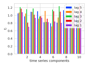
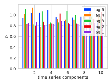
(a) $T=100$

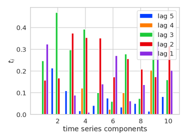
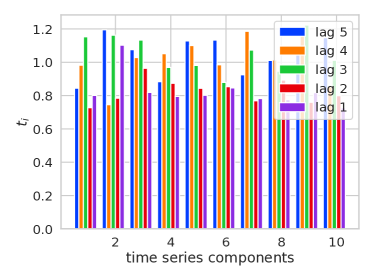
(b) $T=200$

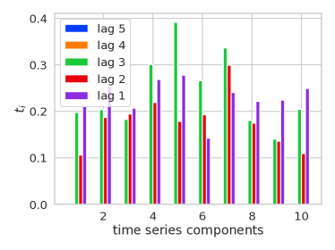
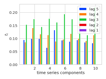
(c) $T=1000$

Figure 3: Comparison of learned Granger causality coefficients $t_{i}$’s of 10 dimensional VAR dataset using the cLSTMwF model. (Left) Ground truth lags are $1,2$ and $3$, (right) ground truth lags are $3,4$ and $5$.

9.1 VAR(3) model

We conclude a preliminary experimental study to assess how well can neural networks model perform on the relatively simple task of fitting 10-dimensional VAR(3), i.e., linear model, with $20\%$ of time series components being causal.

Considering the performance of each method, we include a linear VAR model to provide an upper bound of how good the performance could be. We can see a similar performance for component-wise models with the marginally superior performance of LSTM based models, at least in terms of AUROC. We see that our decoupling strategy can improve performance when we compare cLSTM and cLSTMwF for $T=200$.

Note that all the methods solve the problem perfectly when they have access to one thousand data samples.

We realize that the performance of all the methods is very similar, i.e., within one or few standard errors, which is a good sign as we include VAR as one of our baselines, showing the flexibility of the neural network-based methods.

To showcase that we can extract lags in recurrent neural network with our new framework introduced in Section 7, we displayed obtained $t_{i}$’s coefficient for the cLSTMwF model. To further showcase flexibility, we also generate data where the lags 3, 4 and 5 are causal. Figure 3 displays the obtained $t_{i}$’s coefficient and shows that it is indeed the case that for the sufficiently large number of data, our approach is able to exactly recover the underlying lag structure.

9.2 Lorenz-96 Model

Table 2: Comparison of AUROC and AUPR for Granger causality selection among 20 dimensional Lorenz-96 model, parametrised as a function of the length of the time series $T$. Results are the mean across three initializations, with one standard deviation.

	AUROC			AUPR
T	250	750	1500	100	200	1000
VAR	83.9 ± 0.4	96.7 ± 0.1	99.1 ± 0.1	71.0 ± 0.3	93.2 ± 0.3	97.0 ± 0.2
LeKVAR	84.5 ± 0.6	94.8 ± 3.1	100.0 ± 0.0	71.1 ± 2.8	91.5 ± 3.9	99.9 ± 0.0
cMLP	88.5 ± 0.4	97.6 ± 0.5	99.9 ± 0.0	77.2 ± 0.5	95.2 ± 0.5	99.8 ± 0.1
cMLPwF	89.8 ± 1.3	94.7 ± 0.2	90.4 ± 2.5	78.0 ± 1.5	92.6 ± 0.9	84.9 ± 3.8
cLSTM	50.8 ± 3.3	73.0 ± 2.3	98.2 ± 0.6	22.8 ± 2.3	43.4 ± 2.1	92.3 ± 2.4
cLSTMwF	54.4 ± 3.9	91.6 ± 2.3	97.9 ± 0.1	24.3 ± 2.7	76.7 ± 7.6	90.6 ± 0.8
cMLP_s	92.0 ± 0.3	96.1 ± 0.8	99.8 ± 0.1	79.6 ± 0.4	88.4 ± 4.1	99.3 ± 0.4
cMLPwF_s	88.4 ± 1.4	99.0 ± 0.3	99.5 ± 0.0	75.0 ± 3.7	97.0 ± 0.6	98.0 ± 0.1
cLSTM_s	56.6 ± 3.5	96.6 ± 0.6	99.1 ± 0.1	25.6 ± 4.2	91.0 ± 1.2	96.4 ± 0.6
cLSTMwF_s	58.3 ± 0.5	87.8 ± 1.2	98.4 ± 0.2	25.8 ± 0.5	56.1 ± 4.2	93.1 ± 1.0

The continuous dynamics in a $p$-dimensional Lorenz model are given by

$$\frac{dx_{ti}}{dt}=\left(x_{t(i+1)}-x_{t(i-2)}\right)x_{t(i-1)}-x_{ti}+F,$$ (11)

where $x_{t(-1)}=x_{t(p-1)},x_{t0}=x_{tp},x_{t(p+1)}=x_{t1}$ and $F$ is a forcing constant that determines the level of nonlinearity and chaos in the series. We numerically simulate a $p=20$ Lorenz-96 model with a sampling rate of $\Delta_{t}=0.05$ and $F=20$, which results in a multivariate, nonlinear time series with sparse Granger causal connections.

As previously, using this simulation setup, we test our models’ ability to recover the underlying causal structure. Average values of area under the ROC curve (AUROC) for recovery of the causal structure across five initialization seeds are shown in Table 2, and we obtain results under three different data set lengths, $T\in(250,750,1500)$.

As expected, the results indicate that all models improve as the data set size $T$ increases. The MLP-based models outperform their LSTM-based counterparts, but the gap in their performance narrows as more data is used. In the low data regime, the performance is dominated by small neural network-based models, but the order is swapped for the dataset with 1500 samples. We see the mixed effect of decoupling. Often decoupling brings no improvement. Upon looking at the tuned parameters, we appoint this to imperfect tuning as decoupling usually reaches its limit at the extreme value of our predefined regularization parameters. In contrast, the methods with no decoupling tend to choose non-edge values.

Table 3: Comparison of AUPR for Granger causality selection among 100 dimensional gene expression data from Dream Challenge. Results are the mean across three initializations, with one standard deviation.

AUPR
Dataset	Ecoli1	Ecoli12	Yeast1	Yeast2	Yeast3
VAR	29.2 ± 0.4	29.8 ± 1.2	27.6 ± 0.9	20.5 ± 0.4	17.6 ± 0.0
LeKVAR	2.5 ± 0.8	3.5 ± 2.1	11.1 ± 5.0	4.9 ± 0.9	11.3 ± 4.8
cMLP	38.5 ± 1.4	37.9 ± 0.6	39.4 ± 1.6	24.1 ± 0.2	21.8 ± 0.5
cMLPwF	35.7 ± 0.2	17.0 ± 1.7	37.5 ± 1.1	25.0 ± 1.5	21.1 ± 0.2
cLSTM	30.8 ± 0.4	35.6 ± 1.3	31.6 ± 0.9	23.0 ± 1.1	21.2 ± 1.0
cLSTMwF	22.7 ± 3.0	22.0 ± 2.6	25.7 ± 0.5	18.3 ± 0.6	17.2 ± 0.5
cMLP_s	25.2 ± 0.1	23.1 ± 0.9	45.6 ± 0.8	30.3 ± 0.3	24.9 ± 0.5
cMLPwF_s	46.7 ± 1.0	42.3 ± 1.5	42.2 ± 0.9	27.4 ± 0.7	23.3 ± 0.4
cLSTM_s	23.7 ± 0.7	23.4 ± 0.8	32.1 ± 0.4	19.5 ± 0.7	20.2 ± 0.3
cLSTMwF_s	18.9 ± 0.4	17.7 ± 2.4	23.7 ± 1.6	15.7 ± 0.4	17.6 ± 0.4

9.3 DREAM Challenge

We next apply our methods to estimate Granger causality networks from a realistically simulated time course gene expression data set. The data are from the DREAM3 challenge  (Prill et al., 2010) and provide a difficult, non-linear data set for rigorously comparing Granger causality detection methods Lim et al. (2015); Lèbre (2009). The data is simulated using continuous gene expression and regulation dynamics, with multiple hidden factors that are not observed. The challenge contains five different simulated data sets, each with different ground truth Granger causality graphs: two E. Coli (E.C.) data sets and three Yeast (Y.) data sets. Each data set contains $p=100$ different time series, each with $46$ replicates sampled at $21$ time points for a total of $966$ time points.

Due to the short length of the series replicates, we choose the maximum lag in the non-recurrent models to be $2$ and we increase the number of training epochs to $1000$. We display the resulting AUPR (more meaningful metric for highly unbalanced classes) across all 5 datasets in Table 3.

These results clearly demonstrate the importance of taking a nonlinear approach to Granger causality detection in a (simulated) real-world scenario. Among the tested models, small cMLP with decoupling (cMLPwF_s) gives either the best or the second best performance. This observation shows importance of adjusting model size to the dataset size as well as efficient technique to extract Granger causal components. We note the LeKVAR perfoms poorly on this baseline, which might have been caused by an insufficient optimization that remains the main challenge of applying NNs for GC. We also observe that MLP-based models performs significantly better LSTM-based ones. This goes against the common findings in the literature where LSTMs outperform autoregressive MLPs. We believe that this issue could be overcome by more extensive tuning and we expect that the LSTM results could be much improved.

9.4 Interesting phenomena

We note that essentially for all experiments, including highly non-linear datasets, the linear VAR is surprisingly a very good baseline. In other words, this means that the first-order Taylor approximation of a complicated underlying true model can be sufficient to estimate dependencies.

We appoint this fact to the following intuitive understanding that we conclude from our experimental results. Firstly, the model does not need to perform well to guess which coefficients are important and which are not. It only needs to decrease the loss by a small value such that the connection to the corresponding component is not pushed to zero by the sparsity-inducing penalty. To support this intuition, we looked at the validation loss and the VAR model was almost always the worst performing model despite being among the best in terms of AUROC.In conclusion, this observation suggests that GC appears to be an easier task than forecasting. In addition, using the VAR model as a preprocessing step might be helpful as it is relatively simple to tune when compared with NNs with many hyperparameters.

9.5 EEG Epilepsy Data

Epilepsy is characterized by recurring seizures, which are marked by a burst of neuronal activity in brain regions that affects the normal functionality of the brain. Brain connectivity is essential for understanding brain function and developing methods for the classification of Neurological Disorders Phang et al. (2019); Kong et al. (2019). We analyze the EEG data utilized in Ombao, Von Sachs and Guo (2005). The EEG data used in this experiment was recorded at a sampling rate of 100Hz recording for 500 seconds. The data was divided into windows of 2000 time points (20 seconds) with a 50% overlap between successive windows. Inside each window 75% of the data was used for training and 25% of the data was used as a holdout set for testing the model. The data was considered for a lag of 3. Each feature was standardized using standard scaling given in 12

$${z_{i,t-k,m}}=\frac{{x_{i,t-k,m}-{\mu_{i,t-k}}}}{s_{i,t-k}}$$ (12)

where $z_{i,t-k,m}$ is the standardized value, at a lag of t-k for the m value in the data,$x_{i,t-k,m}$ is the value to be normalized, $\mu_{i,t-k}$ is the average for the lag of k, and $s_{i,t-k}$ is the sample standard deviation of the training data for the time series $i$. The data was analyzed for GC using cMLPwF, the algorithm was trained using learning rates of [0.001, 0.01] and $\lambda$ values of [1e-5,1e-4,1e-3,1e-2]. The GC was estimated by first normalizing the weights for the features using min max scaler which is given by 13 and using a threshold of 0.5. The GC was then estimated using the model which performed the best on the test data based on mean squared error loss.

$${sc_{i,j}}=\frac{{gc_{i,j}-min_{j}}}{max_{j}-min{j}}$$ (13)

where ${i}$ and ${j}$ refer to the causal and the effected series, $sc_{i,j}$, $gc_{i,j}$ are the scaled and un-scaled values of GC estimates. After applying the method to the data we got interesting results which require further investigation as we continue ti apply our methods to more EEG data. The T3 channel appears to be strongly Granger caused by F7 and the GC changes right at the onset of the seizure where we observe that T3 is no-longer Granger Caused by F7. The seizure starts at around 340 seconds, after the seizure F7 again Granger causes T3 as shown in 5. We observe clear change in the pattern of how T3 Granger causes all channels during the seizure where at 350-seconds we observe that T3 causes all channels which might be an indication of an increase in the electrical activity which can be observed in 4

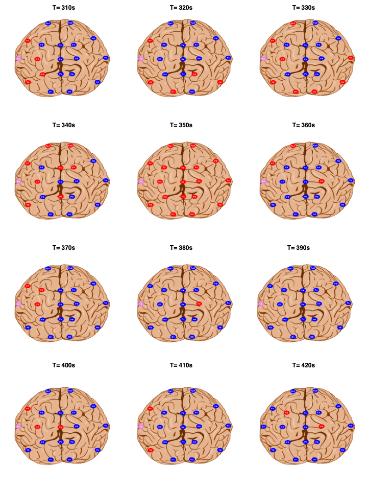
Figure 4: Illustration of the T3 Granger causing other sensors obtained by cMLPwF, T3 is observed to be mostly Granger causing T5 throughout before seizure, however during the seizure from 360 seconds to 400 seconds T3 does not Granger cause T5, T3 also only Granger causes Pz and Fz at the onset of the seizure from 340-350 seconds and does not Granger cause it afterwards for the most part of the EEG recording.

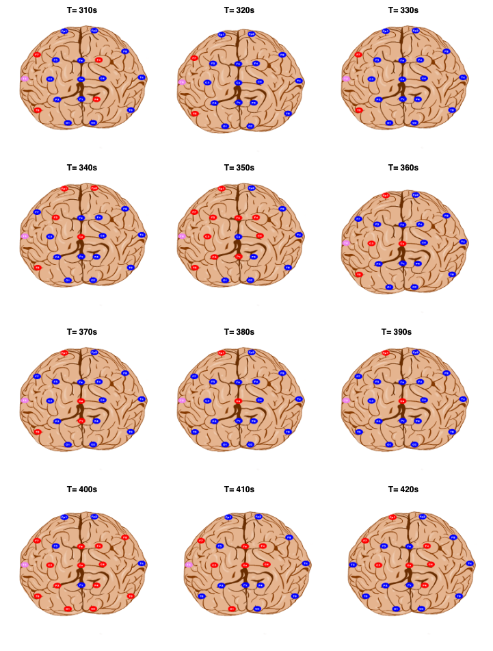
Figure 5: Illustration of the T3 Granger Caused by the other sensors obtained by cMLPwF, T3 is observed to be mostly Granger caused by F7 throughout before seizure, however at the onset and during the seizure it does not GC T3 except at time interval 350 seconds, however at 400 seconds the F7 again starts to GC T3 .

10 Conclusion and Future Work

This paper looks at the different approaches to estimating Granger causality (GC) using neural network models. We start by revising the prior work and identifying several advantages and disadvantages of the previously proposed models. We propose LeKVAR as an extension to the kernel methods where we parameterize the kernel using a neural network model. We include its learning as a part of the training procedure. Furthermore, we develop a new framework that allows us to decouple model selection and Granger causality that provides a lot of promising features, e.g., lag estimates for RNNs and build-in prior knowledge, leading to improved performance in inferring the Granger-causal connections. Next, we identify and fix the issue that the previous approaches to neural Granger causality, including our proposed models, can’t be naively applied as the learning objective is degenerated, i.e., it does not promote sparsity regardless of the sparsity parameter. We also propose a new problem reformulation that enables us to use popular tricks to optimize neural networks. We evaluate the proposed methods on simulated toy and real-world datasets, and we conclude that NN-based models are compatible and can be used to infer Granger causality. However, efficient tuning/optimization techniques remain a formidable challenge that we want to tackle in future work. Apart from this, another promising direction is to extend our approach to account for the uncertainty about the zeroness (we want to control the rate of false negatives) and quantify the uncertainty about the non-zeroness (we want to control the rate of false positives) as the current solution gives only point estimates. Finally, we plan to apply these techniques to real-world data such as EEG measurements to capture changes in brain connectivity.

References

- Amblard and Michel (2011) {barticle}[author] \bauthor\bsnmAmblard, \bfnmPierre-Olivier\binitsP.-O. and \bauthor\bsnmMichel, \bfnmOlivier JJ\binitsO. J. (\byear2011). \btitleOn directed information theory and Granger causality graphs. \bjournalJournal of Computational Neuroscience \bvolume30 \bpages7–16. \endbibitem
- Bach et al. (2012) {barticle}[author] \bauthor\bsnmBach, \bfnmFrancis\binitsF., \bauthor\bsnmJenatton, \bfnmRodolphe\binitsR., \bauthor\bsnmMairal, \bfnmJulien\binitsJ., \bauthor\bsnmObozinski, \bfnmGuillaume\binitsG. \betalet al. (\byear2012). \btitleOptimization with sparsity-inducing penalties. \bjournalFoundations and Trends® in Machine Learning \bvolume4 \bpages1–106. \endbibitem
- Basu et al. (2015) {barticle}[author] \bauthor\bsnmBasu, \bfnmSumanta\binitsS., \bauthor\bsnmMichailidis, \bfnmGeorge\binitsG. \betalet al. (\byear2015). \btitleRegularized estimation in sparse high-dimensional time series models. \bjournalThe Annals of Statistics \bvolume43 \bpages1535–1567. \endbibitem
- Basu, Shojaie and Michailidis (2015) {barticle}[author] \bauthor\bsnmBasu, \bfnmSumanta\binitsS., \bauthor\bsnmShojaie, \bfnmAli\binitsA. and \bauthor\bsnmMichailidis, \bfnmGeorge\binitsG. (\byear2015). \btitleNetwork Granger causality with inherent grouping structure. \bjournalThe Journal of Machine Learning Research \bvolume16 \bpages417–453. \endbibitem
- Billings (2013) {bbook}[author] \bauthor\bsnmBillings, \bfnmStephen A\binitsS. A. (\byear2013). \btitleNonlinear System Identification: NARMAX Methods in the Time, Frequency, and Spatio-Temporal Domains. \bpublisherJohn Wiley & Sons. \endbibitem
- Billings and Chen (1996) {barticle}[author] \bauthor\bsnmBillings, \bfnmSA\binitsS. and \bauthor\bsnmChen, \bfnmS\binitsS. (\byear1996). \btitleThe determination of multivariable nonlinear models for dynamic systems using neural networks. \endbibitem
- Chu, Shoureshi and Tenorio (1990) {barticle}[author] \bauthor\bsnmChu, \bfnmS Reynold\binitsS. R., \bauthor\bsnmShoureshi, \bfnmRahmat\binitsR. and \bauthor\bsnmTenorio, \bfnmManoel\binitsM. (\byear1990). \btitleNeural networks for system identification. \bjournalIEEE Control Systems Magazine \bvolume10 \bpages31–35. \endbibitem
- Fujita et al. (2010) {binproceedings}[author] \bauthor\bsnmFujita, \bfnmAndré\binitsA., \bauthor\bsnmSeverino, \bfnmPatricia\binitsP., \bauthor\bsnmSato, \bfnmJoao Ricardo\binitsJ. R. and \bauthor\bsnmMiyano, \bfnmSatoru\binitsS. (\byear2010). \btitleGranger causality in systems biology: modeling gene networks in time series microarray data using vector autoregressive models. In \bbooktitleBrazilian Symposium on Bioinformatics \bpages13–24. \bpublisherSpringer. \endbibitem
- Granger (1969) {barticle}[author] \bauthor\bsnmGranger, \bfnmClive WJ\binitsC. W. (\byear1969). \btitleInvestigating causal relations by econometric models and cross-spectral methods. \bjournalEconometrica: Journal of the Econometric Society \bpages424–438. \endbibitem
- Hochreiter and Schmidhuber (1997) {barticle}[author] \bauthor\bsnmHochreiter, \bfnmSepp\binitsS. and \bauthor\bsnmSchmidhuber, \bfnmJürgen\binitsJ. (\byear1997). \btitleLong short-term memory. \bjournalNeural computation \bvolume9 \bpages1735–1780. \endbibitem
- Huang, Zhang and Metaxas (2011) {barticle}[author] \bauthor\bsnmHuang, \bfnmJunzhou\binitsJ., \bauthor\bsnmZhang, \bfnmTong\binitsT. and \bauthor\bsnmMetaxas, \bfnmDimitris\binitsD. (\byear2011). \btitleLearning with structured sparsity. \bjournalJournal of Machine Learning Research \bvolume12 \bpages3371–3412. \endbibitem
- Jenatton et al. (2011) {barticle}[author] \bauthor\bsnmJenatton, \bfnmRodolphe\binitsR., \bauthor\bsnmMairal, \bfnmJulien\binitsJ., \bauthor\bsnmObozinski, \bfnmGuillaume\binitsG. and \bauthor\bsnmBach, \bfnmFrancis\binitsF. (\byear2011). \btitleProximal methods for hierarchical sparse coding. \bjournalJournal of Machine Learning Research \bvolume12 \bpages2297–2334. \endbibitem
- Kişi (2004) {barticle}[author] \bauthor\bsnmKişi, \bfnmÖzgür\binitsÖ. (\byear2004). \btitleRiver flow modeling using artificial neural networks. \bjournalJournal of Hydrologic Engineering \bvolume9 \bpages60–63. \endbibitem
- Kim and Xing (2010) {binproceedings}[author] \bauthor\bsnmKim, \bfnmSeyoung\binitsS. and \bauthor\bsnmXing, \bfnmEric P\binitsE. P. (\byear2010). \btitleTree-guided group lasso for multi-task regression with structured sparsity. In \bbooktitleInternational Conference on Machine Learning \bvolume2 \bpages1. \bpublisherCiteseer. \endbibitem
- Kingma and Ba (2014) {barticle}[author] \bauthor\bsnmKingma, \bfnmDiederik P\binitsD. P. and \bauthor\bsnmBa, \bfnmJimmy\binitsJ. (\byear2014). \btitleAdam: A method for stochastic optimization. \bjournalarXiv preprint arXiv:1412.6980. \endbibitem
- Kong et al. (2019) {barticle}[author] \bauthor\bsnmKong, \bfnmYazhou\binitsY., \bauthor\bsnmGao, \bfnmJianliang\binitsJ., \bauthor\bsnmXu, \bfnmYunpei\binitsY., \bauthor\bsnmPan, \bfnmYi\binitsY., \bauthor\bsnmWang, \bfnmJianxin\binitsJ. and \bauthor\bsnmLiu, \bfnmJin\binitsJ. (\byear2019). \btitleClassification of autism spectrum disorder by combining brain connectivity and deep neural network classifier. \bjournalNeurocomputing \bvolume324 \bpages63–68. \endbibitem
- Lèbre (2009) {barticle}[author] \bauthor\bsnmLèbre, \bfnmSophie\binitsS. (\byear2009). \btitleInferring dynamic genetic networks with low order independencies. \bjournalStatistical Applications in Genetics and Molecular Biology \bvolume8 \bpages1–38. \endbibitem
- Li et al. (2017) {barticle}[author] \bauthor\bsnmLi, \bfnmYaguang\binitsY., \bauthor\bsnmYu, \bfnmRose\binitsR., \bauthor\bsnmShahabi, \bfnmCyrus\binitsC. and \bauthor\bsnmLiu, \bfnmYan\binitsY. (\byear2017). \btitleGraph convolutional recurrent neural network: Data-driven traffic forecasting. \bjournalarXiv preprint arXiv:1707.01926. \endbibitem
- Lim et al. (2015) {barticle}[author] \bauthor\bsnmLim, \bfnmNéhémy\binitsN., \bauthor\bsnmD’Alché-Buc, \bfnmFlorence\binitsF., \bauthor\bsnmAuliac, \bfnmCédric\binitsC. and \bauthor\bsnmMichailidis, \bfnmGeorge\binitsG. (\byear2015). \btitleOperator-valued kernel-based vector autoregressive models for network inference. \bjournalMachine Learning \bvolume99 \bpages489–513. \endbibitem
- Lozano et al. (2009a) {binproceedings}[author] \bauthor\bsnmLozano, \bfnmAurelie C\binitsA. C., \bauthor\bsnmAbe, \bfnmNaoki\binitsN., \bauthor\bsnmLiu, \bfnmYan\binitsY. and \bauthor\bsnmRosset, \bfnmSaharon\binitsS. (\byear2009a). \btitleGrouped graphical Granger modeling methods for temporal causal modeling. In \bbooktitleProceedings of the 15th ACM SIGKDD International Conference on Knowledge Discovery and Data Mining \bpages577–586. \bpublisherACM. \endbibitem
- Lozano et al. (2009b) {barticle}[author] \bauthor\bsnmLozano, \bfnmAurélie C\binitsA. C., \bauthor\bsnmAbe, \bfnmNaoki\binitsN., \bauthor\bsnmLiu, \bfnmYan\binitsY. and \bauthor\bsnmRosset, \bfnmSaharon\binitsS. (\byear2009b). \btitleGrouped graphical Granger modeling for gene expression regulatory networks discovery. \bjournalBioinformatics \bvolume25 \bpagesi110–i118. \endbibitem
- Lusch, Maia and Kutz (2016) {barticle}[author] \bauthor\bsnmLusch, \bfnmBethany\binitsB., \bauthor\bsnmMaia, \bfnmPedro D\binitsP. D. and \bauthor\bsnmKutz, \bfnmJ Nathan\binitsJ. N. (\byear2016). \btitleInferring connectivity in networked dynamical systems: Challenges using Granger causality. \bjournalPhysical Review E \bvolume94 \bpages032220. \endbibitem
- Lütkepohl (2005) {bbook}[author] \bauthor\bsnmLütkepohl, \bfnmHelmut\binitsH. (\byear2005). \btitleNew Introduction to Multiple Time Series Analysis. \bpublisherSpringer Science & Business Media. \endbibitem
- Nicholson, Bien and Matteson (2014) {barticle}[author] \bauthor\bsnmNicholson, \bfnmWilliam B\binitsW. B., \bauthor\bsnmBien, \bfnmJacob\binitsJ. and \bauthor\bsnmMatteson, \bfnmDavid S\binitsD. S. (\byear2014). \btitleHierarchical vector autoregression. \bjournalarXiv preprint arXiv:1412.5250. \endbibitem
- Ombao, Von Sachs and Guo (2005) {barticle}[author] \bauthor\bsnmOmbao, \bfnmHernando\binitsH., \bauthor\bsnmVon Sachs, \bfnmRainer\binitsR. and \bauthor\bsnmGuo, \bfnmWensheng\binitsW. (\byear2005). \btitleSLEX analysis of multivariate nonstationary time series. \bjournalJournal of the American Statistical Association \bvolume100 \bpages519–531. \endbibitem
- Parikh et al. (2014) {barticle}[author] \bauthor\bsnmParikh, \bfnmNeal\binitsN., \bauthor\bsnmBoyd, \bfnmStephen\binitsS. \betalet al. (\byear2014). \btitleProximal algorithms. \bjournalFoundations and Trends in Optimization \bvolume1 \bpages127–239. \endbibitem
- Phang et al. (2019) {barticle}[author] \bauthor\bsnmPhang, \bfnmChun-Ren\binitsC.-R., \bauthor\bsnmTing, \bfnmChee-Ming\binitsC.-M., \bauthor\bsnmNoman, \bfnmFuad\binitsF. and \bauthor\bsnmOmbao, \bfnmHernando\binitsH. (\byear2019). \btitleClassification of EEG-based brain connectivity networks in schizophrenia using a multi-domain connectome convolutional neural network. \bjournalarXiv preprint arXiv:1903.08858. \endbibitem
- Prill et al. (2010) {barticle}[author] \bauthor\bsnmPrill, \bfnmRobert J\binitsR. J., \bauthor\bsnmMarbach, \bfnmDaniel\binitsD., \bauthor\bsnmSaez-Rodriguez, \bfnmJulio\binitsJ., \bauthor\bsnmSorger, \bfnmPeter K\binitsP. K., \bauthor\bsnmAlexopoulos, \bfnmLeonidas G\binitsL. G., \bauthor\bsnmXue, \bfnmXiaowei\binitsX., \bauthor\bsnmClarke, \bfnmNeil D\binitsN. D., \bauthor\bsnmAltan-Bonnet, \bfnmGregoire\binitsG. and \bauthor\bsnmStolovitzky, \bfnmGustavo\binitsG. (\byear2010). \btitleTowards a rigorous assessment of systems biology models: the DREAM3 challenges. \bjournalPloS One \bvolume5 \bpagese9202. \endbibitem
- Raissi, Perdikaris and Karniadakis (2018) {barticle}[author] \bauthor\bsnmRaissi, \bfnmMaziar\binitsM., \bauthor\bsnmPerdikaris, \bfnmParis\binitsP. and \bauthor\bsnmKarniadakis, \bfnmGeorge Em\binitsG. E. (\byear2018). \btitleMultistep neural networks for data-driven discovery of nonlinear dynamical systems. \bjournalarXiv preprint arXiv:1801.01236. \endbibitem
- Runge et al. (2012) {barticle}[author] \bauthor\bsnmRunge, \bfnmJakob\binitsJ., \bauthor\bsnmHeitzig, \bfnmJobst\binitsJ., \bauthor\bsnmPetoukhov, \bfnmVladimir\binitsV. and \bauthor\bsnmKurths, \bfnmJürgen\binitsJ. (\byear2012). \btitleEscaping the curse of dimensionality in estimating multivariate transfer entropy. \bjournalPhysical Review Letters \bvolume108 \bpages258701. \endbibitem
- Salimans and Kingma (2016) {barticle}[author] \bauthor\bsnmSalimans, \bfnmTim\binitsT. and \bauthor\bsnmKingma, \bfnmDurk P\binitsD. P. (\byear2016). \btitleWeight normalization: A simple reparameterization to accelerate training of deep neural networks. \bjournalAdvances in neural information processing systems \bvolume29. \endbibitem
- Sameshima and Baccala (2016) {bbook}[author] \bauthor\bsnmSameshima, \bfnmKoichi\binitsK. and \bauthor\bsnmBaccala, \bfnmLuiz Antonio\binitsL. A. (\byear2016). \btitleMethods in Brain Connectivity Inference Through Multivariate Time Series Analysis. \bpublisherCRC Press. \endbibitem
- Sharpe, Alexander and Bailey (1968) {bbook}[author] \bauthor\bsnmSharpe, \bfnmWilliam F\binitsW. F., \bauthor\bsnmAlexander, \bfnmGordon J\binitsG. J. and \bauthor\bsnmBailey, \bfnmJeffrey W\binitsJ. W. (\byear1968). \btitleInvestments. \bpublisherPrentice Hall. \endbibitem
- Sheikhattar et al. (2018) {barticle}[author] \bauthor\bsnmSheikhattar, \bfnmAlireza\binitsA., \bauthor\bsnmMiran, \bfnmSina\binitsS., \bauthor\bsnmLiu, \bfnmJi\binitsJ., \bauthor\bsnmFritz, \bfnmJonathan B\binitsJ. B., \bauthor\bsnmShamma, \bfnmShihab A\binitsS. A., \bauthor\bsnmKanold, \bfnmPatrick O\binitsP. O. and \bauthor\bsnmBabadi, \bfnmBehtash\binitsB. (\byear2018). \btitleExtracting neuronal functional network dynamics via adaptive Granger causality analysis. \bjournalProceedings of the National Academy of Sciences \bvolume115 \bpagesE3869–E3878. \endbibitem
- Simon et al. (2013) {barticle}[author] \bauthor\bsnmSimon, \bfnmNoah\binitsN., \bauthor\bsnmFriedman, \bfnmJerome\binitsJ., \bauthor\bsnmHastie, \bfnmTrevor\binitsT. and \bauthor\bsnmTibshirani, \bfnmRobert\binitsR. (\byear2013). \btitleA Sparse-Group Lasso. \bjournalJournal of Computational and Graphical Statistics \bvolume22 \bpages231-245. \bdoi10.1080/10618600.2012.681250 \endbibitem
- Sporns (2010) {bbook}[author] \bauthor\bsnmSporns, \bfnmOlaf\binitsO. (\byear2010). \btitleNetworks of the Brain. \bpublisherMIT Press. \endbibitem
- Stokes and Purdon (2017) {barticle}[author] \bauthor\bsnmStokes, \bfnmPatrick A\binitsP. A. and \bauthor\bsnmPurdon, \bfnmPatrick L\binitsP. L. (\byear2017). \btitleA study of problems encountered in Granger causality analysis from a neuroscience perspective. \bjournalProceedings of the National Academy of Sciences \bvolume114 \bpagesE7063–E7072. \endbibitem
- Sun (2008) {binproceedings}[author] \bauthor\bsnmSun, \bfnmXiaohai\binitsX. (\byear2008). \btitleAssessing nonlinear Granger causality from multivariate time series. In \bbooktitleJoint European Conference on Machine Learning and Knowledge Discovery in Databases \bpages440–455. \bpublisherSpringer. \endbibitem
- Tank et al. (2018) {barticle}[author] \bauthor\bsnmTank, \bfnmAlex\binitsA., \bauthor\bsnmCovert, \bfnmIan\binitsI., \bauthor\bsnmFoti, \bfnmNicholas\binitsN., \bauthor\bsnmShojaie, \bfnmAli\binitsA. and \bauthor\bsnmFox, \bfnmEmily\binitsE. (\byear2018). \btitleNeural granger causality. \bjournalarXiv preprint arXiv:1802.05842. \endbibitem
- Tao et al. (2018) {barticle}[author] \bauthor\bsnmTao, \bfnmYunzhe\binitsY., \bauthor\bsnmMa, \bfnmLin\binitsL., \bauthor\bsnmZhang, \bfnmWeizhong\binitsW., \bauthor\bsnmLiu, \bfnmJian\binitsJ., \bauthor\bsnmLiu, \bfnmWei\binitsW. and \bauthor\bsnmDu, \bfnmQiang\binitsQ. (\byear2018). \btitleHierarchical attention-based recurrent highway networks for time series prediction. \bjournalarXiv preprint arXiv:1806.00685. \endbibitem
- Teräsvirta et al. (2010) {bbook}[author] \bauthor\bsnmTeräsvirta, \bfnmTimo\binitsT., \bauthor\bsnmTjøstheim, \bfnmDag\binitsD., \bauthor\bsnmGranger, \bfnmClive William John\binitsC. W. J. \betalet al. (\byear2010). \btitleModelling Nonlinear Economic Time Series. \bpublisherOxford University Press Oxford. \endbibitem
- Tibshirani (1996) {barticle}[author] \bauthor\bsnmTibshirani, \bfnmRobert\binitsR. (\byear1996). \btitleRegression shrinkage and selection via the lasso. \bjournalJournal of the Royal Statistical Society: Series B (Methodological) \bvolume58 \bpages267–288. \endbibitem
- Tong (2011) {barticle}[author] \bauthor\bsnmTong, \bfnmHowell\binitsH. (\byear2011). \btitleNonlinear time series analysis. \bjournalInternational Encyclopedia of Statistical Science \bpages955–958. \endbibitem
- Vicente et al. (2011) {barticle}[author] \bauthor\bsnmVicente, \bfnmRaul\binitsR., \bauthor\bsnmWibral, \bfnmMichael\binitsM., \bauthor\bsnmLindner, \bfnmMichael\binitsM. and \bauthor\bsnmPipa, \bfnmGordon\binitsG. (\byear2011). \btitleTransfer entropy—a model-free measure of effective connectivity for the neurosciences. \bjournalJournal of Computational Neuroscience \bvolume30 \bpages45–67. \endbibitem
- Yu et al. (2017) {barticle}[author] \bauthor\bsnmYu, \bfnmRose\binitsR., \bauthor\bsnmZheng, \bfnmStephan\binitsS., \bauthor\bsnmAnandkumar, \bfnmAnima\binitsA. and \bauthor\bsnmYue, \bfnmYisong\binitsY. (\byear2017). \btitleLong-term forecasting using tensor-train RNNs. \bjournalarXiv preprint arXiv:1711.00073. \endbibitem
- Yuan and Lin (2006) {barticle}[author] \bauthor\bsnmYuan, \bfnmMing\binitsM. and \bauthor\bsnmLin, \bfnmYi\binitsY. (\byear2006). \btitleModel selection and estimation in regression with grouped variables. \bjournalJournal of the Royal Statistical Society: Series B (Statistical Methodology) \bvolume68 \bpages49–67. \endbibitem
- Zhang (2003) {barticle}[author] \bauthor\bsnmZhang, \bfnmG Peter\binitsG. P. (\byear2003). \btitleTime series forecasting using a hybrid ARIMA and neural network model. \bjournalNeurocomputing \bvolume50 \bpages159–175. \endbibitem