A Survey of ADMM Variants for Distributed Optimization: Problems, Algorithms and Features

Abstract

By coordinating terminal smart devices or microprocessors to engage in cooperative computation to achieve system-level targets, distributed optimization is incrementally favored by both engineering and computer science. The well-known alternating direction method of multipliers (ADMM) has turned out to be one of the most popular tools for distributed optimization due to many advantages, such as modular structure, superior convergence, easy implementation and high flexibility. In the past decade, ADMM has experienced widespread developments. The developments manifest in both handling more general problems and enabling more effective implementation. Specifically, the method has been generalized to broad classes of problems (i.e., multi-block, coupled objective, nonconvex, etc.). Besides, it has been extensively reinforced for more effective implementation, such as improved convergence rate, easier subproblems, higher computation efficiency, flexible communication, compatible with inaccurate information, robust to communication delays, etc. These developments lead to a plentiful of ADMM variants to be celebrated by broad areas ranging from smart grids, smart buildings, wireless communications, machine learning and beyond. However, there lacks a survey to document those developments and discern the results. To achieve such a goal, this paper provides a comprehensive survey on ADMM variants. Particularly, we discern the five major classes of problems that have been mostly concerned and discuss the related ADMM variants in terms of main ideas, main assumptions, convergence behaviors and main features. In addition, we figure out several important future research directions to be addressed. This survey is expected to work as a tutorial for both developing distributed optimization in broad areas and identifying existing research gaps.

I Introduction

Distributed optimization is gaining importance and popularity in both engineering and computer science for decision making and data processing with the intensifying computation demands [1, 2, 3]. The notion of distributed optimization is to engage dispersed smart devices or microprocessors in collaborative computation to fulfill a certain system-level target. When it comes to an engineering system, distributed optimization is often used to empower subsystems to make decisions locally while interacting with each other to pursue desirable system performance. In the context of computer science, distributed optimization is often utilized to distributed a heavy training task across multiple microprocessors and coordinate them to fulfill a coherent training target. Though the scenarios are diverse, the philosophy of distributed optimization essentially corresponds to breaking a comprehensive mathematical optimization problem into several small-sized subproblems and empowering multiple computing agents to solve the subproblems in a coordinated manner so as to approach an optimal or near-optimal solution of original mathematical optimization.

When the system or problem is in large scale and many practical issues are considered, distributed optimization is often preferred over its centralized counterpart due to many advantages [4]. Specifically, distributed optimization often shows high computation efficiency and favorable scaling property since the computation is distributed to multiple computing agents. In contrast, a centralized method usually relies on a central unit to solve a comprehensive mathematical optimization independently. This is often computationally intensive or intractable considering the time constraints. Besides, distributed optimization can directly utilize locally available information generated by distributed sensing and monitoring. Whereas a centralized counterpart has to collect information of an entire system (often geographically dispersed) and store massive data in an unified memory for computation. These highlight the multiplied advantages of distributed optimization, such as high computation efficiency, low communication overheads, low footprint memory, and high data privacy.

The well-known alternating direction method of multipliers (ADMM) has emerged as one of the most popular tools for distributed optimization. It has found massive applications in broad areas ranging from statistical learning [5, 6], multi-agent reinforcement learning [7], imaging processing [8, 9], data mining [10, 11], power system control [12, 13, 14, 15], smart grid operation [16, 17, 18, 19, 20, 21, 22], smart building management [23, 24, 25], multi-robot coordination [26], wireless communication control [27, 28], autonomous vehicle routing [29, 30] and beyond. The popularity of ADMM can be attributed to its many distinguishing advantages, such as modular structure, superior convergence, easy implementation and high flexibility. The modular structure characterizes that ADMM generally explores the decomposition of a large-scale optimization across objective components (often called features). This results in a fixed number of subproblems. Each subproblem corresponds to one objective function (one feature) and one disjoint block of decision variables. Afterwards, the subproblems can be handled separately by individual agents using customized solvers. The superiors convergence describes both the less restrictive convergence conditions and faster convergence rates of ADMM over many other distributed methods. For example, ADMM does not entail any smoothness for convex optimization. Besides, ADMM ensures an $\mathcal{O}(1/k)$ convergence rate for convex optimization whereas subgradient methods only promise $\mathcal{O}(1/\sqrt{k})$ convergence rate [31]. ADMM is often more reliable and robust in convergence compared with dual ascent methods at the lack of strong convexity [5]. In addition, ADMM often requires less iterations to approach an optimal or near-optimal solution than distributed gradient methods [32]. Note that the number of iterations often determines the communication overhead of a distributed method. Overall, ADMM has been recognized at least comparable to very specialized algorithms [5]. ADMM enables easy implementation due to the rather small dependence on parameter settings compared with many other distributed methods. This is largely attributed to the quadratic penalty terms that enhance problem convexity. Besides, the subproblems of ADMM often admit closed-form solutions, yielding low per-iteration complexity. The high flexibility can be perceived from the broad classes of problems that can be handled by ADMM either naturally or by means of reformulations. This will be clear from the rest of this paper.

With the growing demand for distributed optimization, ADMM has experienced widespread developments in the past decade. An overview of the developments is shown in Fig. 1. Specifically, the developments manifest in both handling more general problems (i.e., multi-block, coupled objective, nonconvex, etc.) and enabling more effective implementation. Primarily, the method was developed for convex optimization with a two-block separable structure. Whereas it has been generalized to diverse structured convex and nonconvex optimization, which includes i) two-block with separable objective ($\mathbf{P1}$), ii) multi-block with separable objective ($\mathbf{P}2$), iii) multi-block with coupled objective ($\mathbf{P}3$), iv) consensus optimization ($\mathbf{P}4$), and v) non-linearly constrained optimization ($\mathbf{P}5$). In addition, the method has been extensively reinforced for more effective implementation, such as improved convergence rate, easier implementation, higher computation efficiency, flexible communication, compatible with inaccurate information, robust to communication delays, etc.

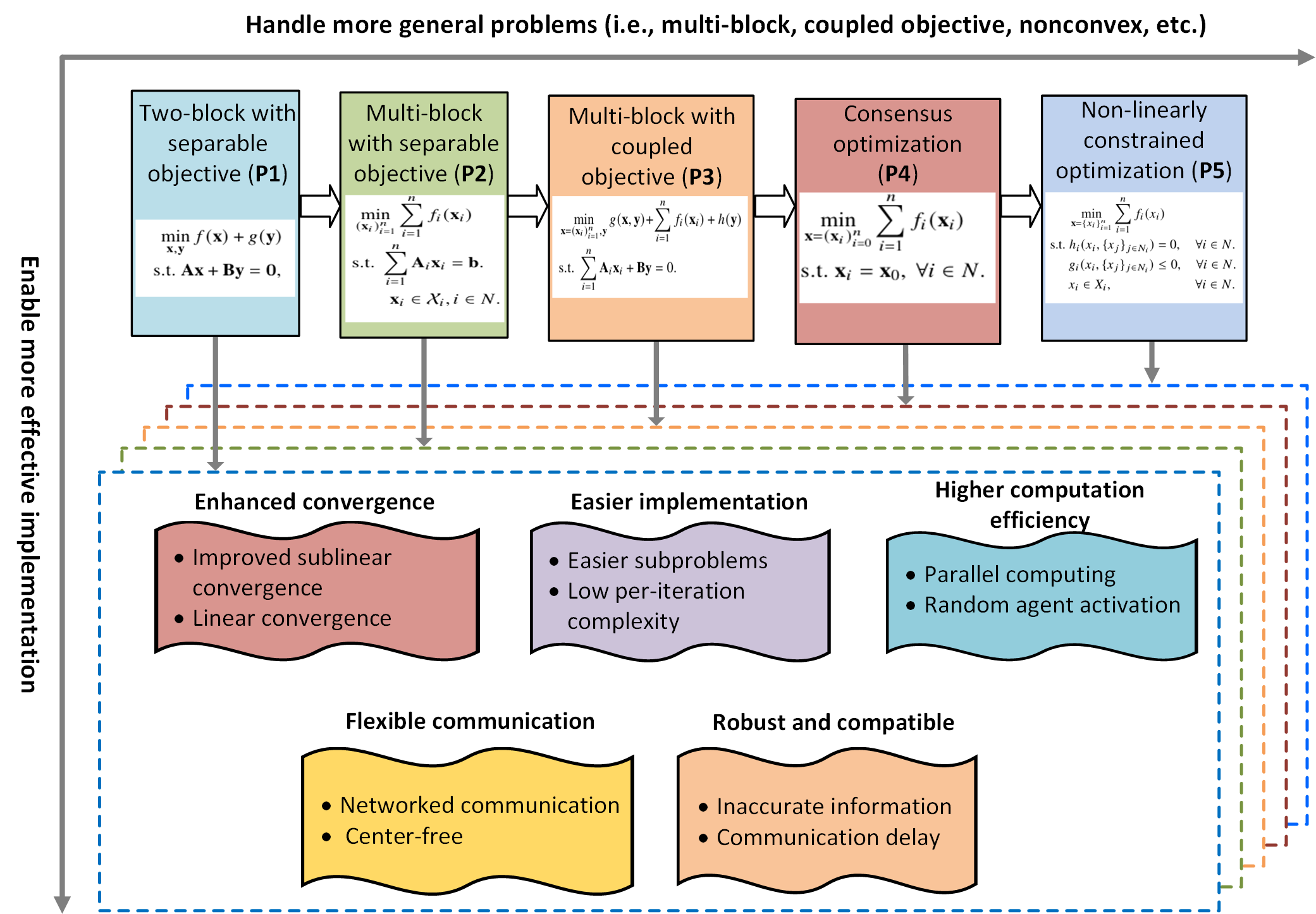
Figure 1: Developments of ADMM for both handling more general problems and enabling more effective implementation.

These developments lead to a plentiful of ADMM variants that are suitable for different problems or situations. Though some of those ADMM variants have found successful applications, many of the them are still limited to the theoretical research community and expected to enjoy broader applications and success. This is mainly caused by the fairly large number of variants developed for different problems and under different conditions, making it rather difficult for one who lacks strong theoretical background to identify an appropriate one for their problems. There lacks a survey to document those developments and discern the results. To fulfill the gap, this paper provides a comprehensive survey on ADMM variants for distributed optimization. Specifically, this paper makes the following main contributions.

• We survey ADMM and its variants developed throughout the decades broadly and comprehensively in both convex and nonconvex settings.

• We discern the five major classes of problems that have been mainly concerned and discuss the related ADMM variants in terms of main assumptions, decomposition scheme, convergence properties and main features.

• Based on the existing results, we figure out the important future research directions to be addressed.

This paper focuses on ADMM and its variants for distributed optimization as they are being incrementally attractive and popular to account for the growing computation demand of broad areas. Though a number of celebrated reviews on distributed optimization have discussed ADMM, most of them only focused on classical ADMM for two-block convex optimization and the significant developments that occurred in very recent decade haven’t been covered yet. We report those reviews in TABLE I by years. Particularly, we distinguish this paper and those reviews by the convexity of concerned problems (Convexity), the presence of constraints (Constraints), the formulations of concerned problems (Problems), the classification criterion (Classification), the related distributed methods (Methods), the specialized applications (Specialized applications) and the year of publication (Year). Note that many of the reviews only involved classical ADMM as one distributed solution. Moreover, they were mainly concerned with convex optimization. As highlighted, there exist five exceptional reviews that are specialized to ADMM like this paper. However, they are in quite different perspectives.

• Boyd et.al. [5] (2011) gave the earliest tutorial on classical ADMM, which documented the fundamental theory of ADMM for convex optimization followed by some applications arising from statistical and machine learning. This tutorial exactly renewed ADMM and raised the surge of interest in the method for distributed optimization.

• Glowinski [33] (2014) gave a introductory review on the origination of ADMM. Specifically, the method originated from an inexact implementation of augmented Lagrangian method (ALM) for solving partial differential equations (PDE). Afterwards, the relationship between the inexact ALM and Douglas-Rachford alternating direction method was discovered, leading to the ADMM that is well-known today.

• Eckstein et.al. [34] (2015) gave a thorough overview on understanding and establishing the convergence of ADMM from the perspective of operator splitting. Specially, this paper argued that ADMM is actually not an approximate ALM as commonly recognized considering its quite different convergence behaviors from the real approximate ALM variants observed in some numerical studies.

• Maneesha et.al. [16] (2021) conducted a survey on the applications of ADMM to smart grid operation. The classical ADMM was introduced in details, followed by its diverse applications to smart grids (e.g., optimal power flow control, economic dispatch, demand response, etc.).

• Han et.al. [35] (2021) gave a comprehensive survey on the recent developments of ADMM and its variants from the perspective of parameter selecting, easier subproblems, approximate iteration, convergence rate characterizations, multi-block and nonconvex extensions.

TABLE I: Existing reviews on distributed optimization that involve ADMM.

References	Convexity	Constraints	Problems	Classification	Methods	Specialized applications	Year
[31]	Convex	Unconstrained Constrained	$\mathbf{P1}$, $\mathbf{P}2$, $\mathbf{P}4$	Problems. Methods.	Gradient method. Subgradient method. Incremental subgradient method. Dual decomposition. Primal decomposition. Classical ADMM.	Game theory. Networked system.	2010
						Data analysis
[5]	Convex	Constrained	$\mathbf{P1}$	–	Classical ADMM	Statistical learning.	2011
[33]	Convex	Constrained	$\mathbf{P1}$	–	Classical ADMM.	–	2014
[34]	Convex	Constrained	$\mathbf{P1}$	–	Classical ADMM.	–	2015
[36]	Convex	Unconstrained Constrained	–	Applications.	Classical ADMM. Dual Decomposition. ATC.	Power system operation	2017
[12]	Convex	Constrained	$\mathbf{P1}$, $\mathbf{P}2$	Methods. Applications.	Dual decomposition. Classical ADMM. ATC. Proximal Message Passing. Consensus+Innovation.	Electrical power system operation.	2017
[37]	Convex	Unconstrained	$\mathbf{P}4$	Problems. Methods.	Distributed average-weighting algorithm. Classical ADMM.	–	2018
[38]	Convex	Unconstrained Constrained	$\mathbf{P}2$, $\mathbf{P}4$	Problems. Methods. Applications.	Distributed subgradient methods. Dual decomposition. Classical ADMM. Distributed dual subgradient methods. Constraints exchange.	Cyber-physical Network	2019
[39]	Convex	Unconstrained Constrained	$\mathbf{P}3$	Methods.	Gradient methods. Subgradient methods. Classical ADMM.	–	2021
[13]	Convex	Constrained	$\mathbf{P}2$	Methods. Applications.	Dual ascent. Primal-dual method. Proximal Atomic Coordination. Classical ADMM.	Electric distribution system control.	2021
[16]	Convex	Constrained	–	Applications.	Classical ADMM	Smart grid operation.	2021
[35]	Convex Nonconvex	Unconstrained Constrained	$\mathbf{P}2$	–	Classical ADMM. ADMM variants.	–	2021
This work	Convex Nonconvex	Unconstrained Constrained	$\mathbf{P1}$, $\mathbf{P}2$, $\mathbf{P}3$, $\mathbf{P}4$, $\mathbf{P}5$	Problems Methods. Features	Classical ADMM. ADMM variants.	–	2022

Notes: we highlight the reviews that focused on ADMM and its variants in gray.

To the authors’ best knowledge, [35] has been the most updated and comprehensive survey on ADMM variants. However, this paper differs from [35] in various aspects. First of all, we make an effort to involve the broad classes of problems (i.e., multi-block, coupled objective, non-linearly constrained, etc.) that have been studied whereas [35] only considered the standard linearly constrained multi-block optimization that represents one class of this paper. Besides, we discern the results from a quite different perspective including problems, methods and features (i.e., parallel computation, low per-iteration complexity, fast convergence, etc.). Specifically, have been able to identify the five major classes of problems that have been mainly concerned in the literature. We then comprehensively discuss the related ADMM variants for each class of problems in terms of main assumptions, decomposition scheme, convergence behaviors and main features. This is relevant to help advance the transfer of ADMM related theory to practice considering that one often intends to search for appropriate distributed solutions by their problems and requirements. In contrast, [35] organized the results by parameter selection, easier subproblems, approximate iteration, convergence rate characterization, multi-block and nonconvex extensions. Based on our experience, this review is more suitable for those who have quite solid theoretical backgrounds on ADMM and its variants. Last but importantly, we comprehensively survey and discuss ADMM variants for nonconvex optimization whereas [35] only gave a short and simple discussion on that topic.

The rest of this survey is as follows. In Section II, we introduce some basic and fundamental knowledge related to ADMM and its variants, which include augmented Lagrangian method (ALM), decomposition techniques, convergence rate characterization, ergodic and nonergodic concepts of convergence. Afterwards, we clarify the mathematical notations frequently used in this paper. In Section III, we introduce classical ADMM and its related theoretical results. In Section IV, we survey ADMM variants for solving the five major classes of problems ($\mathbf{P1}$) - ($\mathbf{P}5$). For each class of problems, we discuss the related ADMM variants from the perspectives of main assumptions, decomposition schemes, convergence properties and main features. In Section V, we discuss several important and promising future research directions. A roadmap for the above major sections (Section II-Section V) is shown in Fig. 2. In Section VI, we conclude this paper.

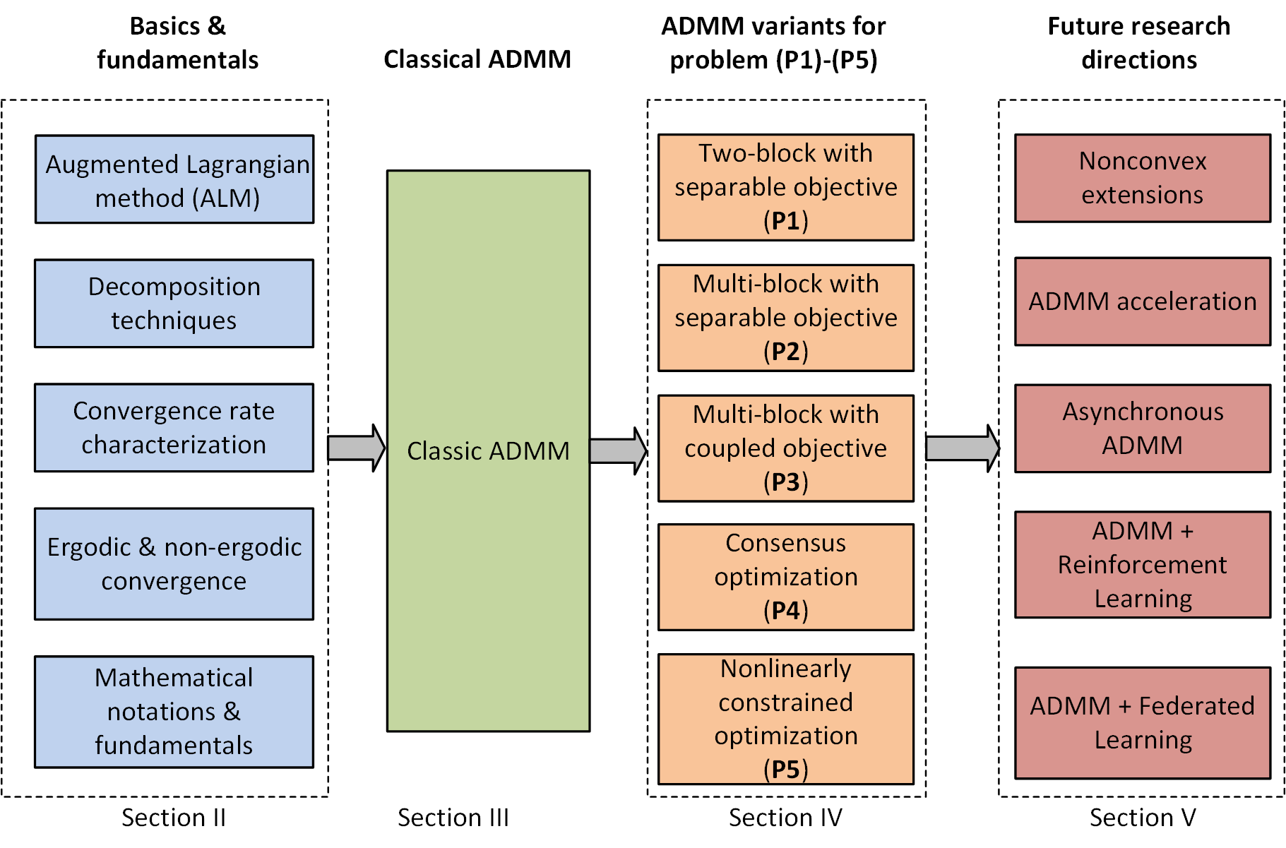
Figure 2: A roadmap for the major sections of this paper (Section II-Section V).

II Basics and Fundamentals

In this section, we first introduce augmented Lagrangian method (ALM) and some decomposition techniques which are the basics of ADMM and its variants. We then introduce convergence rate characterization and ergodic/nonergodic convergence. We finally define the mathematical notions.

II-A Augmented Lagrangian Method

Augmented Lagrangian method (ALM), also known as method of multipliers, is a basic tool for constrained optimization. ALM is the precursor of ADMM. More specifically, ADMM was primarily developed as an approximate implementation of ALM [33].

Central to ALM is to relax some or all constraints of a constrained problem by Lagrangian multipliers and penalty functions (usually quadratic) and then solve a sequence of unconstrained or partially constrained relaxed problems to approach an optimal or near-optimal solution of the original problem. We use a simple linearly constrained optimization to illustrate the idea, i.e.,

$$~{}\min_{\mathbf{x},\mathbf{y}}f(\mathbf{x})+g(\mathbf{y})~{}~{} \mathbf{P1}$$ ()

$${\rm s.t.~{}}\mathbf{A}\mathbf{x}+\mathbf{B}\mathbf{y}=\bm{0},$$

where $f:\mathbf{R}^{n}\rightarrow\mathbf{R}$ and $g:\mathbf{R}^{n}\rightarrow\mathbf{R}$ are given objective functions related to decision variables $\mathbf{x}\in\mathbf{R}^{n}$ and $\mathbf{y}\in\mathbf{R}^{n}$ respectively; $\mathbf{A}\in\mathbf{R}^{l\times n}$ and $\mathbf{B}\in\mathbf{R}^{l\times n}$ are coefficient matrices encoding the linear constraints.

Considering the difficulty to solve the constrained optimization ($\mathbf{P1}$) directly, ALM proposes to relax the constraints by Lagrangian multipliers and penalty functions. Specifically, associating the Lagrangian multipliers $\bm{\lambda}\in\mathbf{R}^{l}$ and quadratic penalty parameter $\rho>0$ with the linear constraints, we have the augmented Lagrangian (AL) function

$$\mathcal{L}_{\rho}(\mathbf{x},\mathbf{y},\bm{\lambda})=f(\mathbf{x})+g(\mathbf{y})+\langle\bm{\lambda},\mathbf{A}\mathbf{x}+\mathbf{B}\mathbf{y}\rangle+\frac{\rho}{2}\|\mathbf{A}\mathbf{x}+\mathbf{B}\mathbf{y}\|^{2}.$$

ALM then performs the following primal-dual updates to approach an optimal or near-optimal solution of ($\mathbf{P1}$).

$$\textbf{Primal update:}~{}~{}~{}(\mathbf{x}^{k+1},\mathbf{y}^{k+1})=\arg\min_{\mathbf{x},\mathbf{y}}\mathcal{L}_{\rho_{k}}(\mathbf{x},\mathbf{y},\bm{\lambda}^{k})$$ (1)

$$\textbf{Dual update:}~{}~{}~{}~{}~{}\bm{\lambda}^{k+1}=\bm{\lambda}^{k}+\rho_{k}(\mathbf{A}\mathbf{x}^{k+1}+\mathbf{B}\mathbf{y}^{k+1})$$ (2)

where $k$ denotes the iteration; $\rho_{k}$ represents some varying penalty parameters which may be preselected or dynamically generated in the iterative process. ALM is composed of two alternative steps: Primal update solves AL problems with given Lagrangian multipliers $\bm{\lambda}^{k}$, and Dual update updates Lagrangian multipliers $\bm{\lambda}^{k}$ based on the obtained solutions. The dual update formula (2) can be interpreted as a dual gradient ascent step with stepsize $\rho_{k}$. Specifically, we have the dual of AL problem $d(\bm{\lambda}^{k})=\min_{\mathbf{x},\mathbf{y}}\mathcal{L}_{\rho_{k}}(\mathbf{x},\mathbf{y},\bm{\lambda}^{k})$ and its gradient $\nabla d(\bm{\lambda}^{k})=\mathbf{A}\mathbf{x}^{k+1}+\mathbf{B}\mathbf{y}^{k+1}$ [40], thereby a dual ascent step for maximizing $d(\bm{\lambda})$ reads as $\bm{\lambda}^{k+1}=\bm{\lambda}^{k}+\rho_{k}(\mathbf{A}\mathbf{x}^{k+1}+\mathbf{B}\mathbf{y}^{k+1})$.

ALM was first proposed by Hestenes [41] and Powell [42] in the 1969s as an alternative to the penalty method for constrained optimization. For the penalty method, the Lagrangian multipliers are absent ($\bm{\lambda}^{k}=0$). The motivation of developing ALM is that penalty method generally requires to increase the penalty parameter $\rho_{k}$ to be very large (e.g., infinity), making the resulting relaxed problems ill-conditioning and very difficult to solve. Moreover, the method was found to be very sensitive to the round-off error caused by the means of analogy computing at that time. In such context, ALM proposes to add Lagrangian multipliers to the objective of penalty method. It was found that when the Lagrangian multipliers are close to its corresponding optima, one does not require quite large penalty parameters, alleviating the difficulty of ill-conditioning.

ALM can be viewed as the combination of penalty method ($\bm{\lambda}^{k}=0$) and Lagrangian method ($\rho_{k}=0$). Lagrangian method was primarily proposed with the idea of obtaining optimal solutions by solving the equations of optimality conditions of a constrained optimization. Since the equations involve primal-dual variables and usually do not admit analytical solutions, a primal-dual iterative update scheme is often used by Lagrangian method to approach the solutions gradually. The implementation of Lagrangian method also falls into the general primal-dual framework (1)-(2) but with zero penalty parameter (i.e., $\rho_{k}=0$) in the primal update and general stepsize $\rho_{k}=\alpha_{k}$ in the dual update. Despite both penalty method and Lagrangian method have found wide applications, they suffer from different drawbacks and limitations. While penalty method tends to face the ill-conditioning issue, Lagrangian method is often very sensitive to the dual stepsize settings. Moreover, Lagrangian method depends on fairly restrictive conditions to ensure convergence, such as local or global convexity over the constrained subsets.

As a combination, ALM moderates the disadvantages of penalty method and Lagrangian method. On one hand, ALM does not require to increase the penalty parameters to be very large and a small fixed one often works quite well, thereby alleviating the ill-conditioning problem with penalty method [43]. On the other hand, ALM often shows smaller dependence on the parameters, such as penalty parameters. It was found that any penalty parameters over certain threshold are admissible to ensure convergence of the method (Prop. 2.4, Ch2, [43]). Besides, ALM often ensures the existence of minimizer of AL problems, which is not provided by penalty method and Lagrangian method as often. Moreover, the Lagrangian multipliers of ALM often converge faster to the optima than that of Lagrangian method and the corresponding terms of penalty method, implying a faster convergence rate with ALM over the other two.

Because of those attractive features, ALM has emerged as one of the most important and popular tools for constrained optimization. The idea and basic theory of ALM have been comprehensively documented in the textbooks authored by Bertsekas [43] and Bergin [44]. We refer the interested readers there for more details.

II-B Decomposition techniques

Despite the benefits, one major drawback of ALM is its nondecomposable structure caused by penalty functions. Consider ($\mathbf{P1}$) as an example, though the objective functions are separable across the decision variables $\mathbf{x}$ and $\mathbf{y}$, we still require to deal with the joint optimization (1) due to the quadratic penalties. The joint optimization is usually difficult, at least not much easier than the original constrained optimization. To overcome such drawback, ALM is often combined with certain decomposition techniques to break the joint optimization into small subproblems. This idea exactly leads to ADMM and its variants to be discussed. There are two widely used decomposition techniques for ALM. One is $\operatorname{Gauss-Seidel}$ decomposition and the other one is $\operatorname{Jacobian}$ decomposition.

II-B1 Gauss-Seidel decomposition

For a joint optimization, $\operatorname{Gauss-Seidel}$ decomposition (also known as alternating minimization) proposes to update the decision variables one by one. Specifically, when $\operatorname{Gauss-Seidel}$ decomposition is applied to the joint primal update (1), we have

$$\textbf{$\mathbf{x}$-update:}~{}\mathbf{x}^{k+1}=\arg\min_{\mathbf{x}}\mathcal{L}_{\rho}(\mathbf{x},\mathbf{y}^{k},\bm{\lambda}^{k})$$

$$\textbf{$\mathbf{y}$-update:}~{}\mathbf{y}^{k+1}=\arg\min_{\mathbf{y}}\mathcal{L}_{\rho}(\mathbf{x}^{k+1},\mathbf{y},\bm{\lambda}^{k})$$

Note that the joint optimization breaks into two serial block updates. $\operatorname{Gauss-Seidel}$ decomposition resembles block coordinate method in the sense that multiple decision variables are optimized one by one by assuming the others with latest updates.

II-B2 Jacobian decomposition

For a joint optimization, $\operatorname{Jacobian}$ decomposition proposes to update the decision variables separately but in parallel by using the previous updates of the others. Specifically, when the $\operatorname{Jacobian}$ decomposition is employed to the joint primal update (1), we have

$$\textbf{$\mathbf{x}$-update}:~{}\mathbf{x}^{k+1}=\arg\min_{\mathbf{x}}\mathcal{L}_{\rho}(\mathbf{x},\mathbf{y}^{k},\bm{\lambda}^{k})$$

$$\textbf{$\mathbf{y}$-update}:~{}\mathbf{y}^{k+1}=\arg\min_{\mathbf{y}}\mathcal{L}_{\rho}(\mathbf{x}^{k},\mathbf{y},\bm{\lambda}^{k})$$

Essentially, both $\operatorname{Gauss-Seidel}$ and $\operatorname{Jacobian}$ decomposition are expected to run multiple rounds to approach an optimal or near-optimal solution of the joint optimization. However, when combined with ALM that already takes an iterative primal-dual scheme, $\operatorname{Gauss-Seidel}$ and $\operatorname{Jacobian}$ decomposition are often performed only once to reduce computation. Clearly, this only provides an approximate solution (may be very rough) to the joint primal update. That is why ADMM and its variants resulting from the combination of ALM and these decomposition techniques are often viewed as inexact or approximate ALM.

One may note that one obvious advantage of $\operatorname{Jacobian}$ over $\operatorname{Gauss-Seidel}$ decomposition for distributed optimization is the parallelizable implementation. However, this usually comes at a cost of being more likely to diverge. This is because a $\operatorname{Jacobian}$ decomposition usually provides a less accurate approximation to a joint primal update of ALM [45, 46].

We has illustrated how $\operatorname{Gauss-Seidel}$ and $\operatorname{Jacobian}$ decomposition are usually combined with ALM to enable distributed computation by a two-block example. This idea is readily extended to general multi-block optimization, which will be commonly seen in the rest of this paper.

II-C Convergence rate characterization

In distributed optimization where an iterative scheme is often used to achieve the coordination of multi-agent computation, convergence rate is an important metric for characterizing the computation efficiency of an algorithm. In the following, we give the definitions of sublinear and linear convergence that will be frequently referred to in this paper.

Definition 1

(Sublinear convergence)  Supposed we have a sequence $\{\mathbf{x}^{k}\}_{k=0}^{K}$ converge to the limit point $\mathbf{x}^{*}$ according to

$$\lim_{k\rightarrow\infty}\frac{\|\mathbf{x}^{k+1}-\mathbf{x}^{*}\|}{\|\mathbf{x}^{k}-\mathbf{x}^{*}\|}=1,$$

we say that the sequence $\{\mathbf{x}^{k}\}_{k=0}^{K}$ converges at a sublinear convergence rate.

Definition 2

(Linear convergence) Suppose we have a sequence $\{\mathbf{x}^{k}\}_{k=0}^{K}$ converge to the limit point $\mathbf{x}^{*}$ according to

$$\lim_{k\rightarrow\infty}\frac{\|\mathbf{x}^{k+1}-\mathbf{x}^{*}\|}{\|\mathbf{x}^{k}-\mathbf{x}^{*}\|}=C,$$

where $C\in(0,1)$ is a constant, we say that the sequence $\{\mathbf{x}_{k}\}_{k=0}^{K}$ converges at linear convergence rate.

ADMM and its many variants promise sublinear convergence in the forms of $\mathcal{O}(1/k)$ or $\mathcal{O}(1/\epsilon)$, $\mathcal{O}(1/k^{2})$ or $\mathcal{O}(1/\sqrt{\epsilon})$, where $k$ is the iteration counter and $\epsilon$ is a solution accuracy. Those convergence rates are often associated with the (worst-case) iteration complexity of a distributed method. A (worst-case) iteration complexity $\mathcal{O}(1/k)$ or $\mathcal{O}(1/\epsilon)$ states that the solution accuracy of the generated sequence would be the order $\mathcal{O}(1/k)$ after $k$ iterations, or equivalently it would require at most $\mathcal{O}(1/\epsilon)$ iterations to approach a solution of accuracy $\epsilon$. Despite those convergence rate characterizations are in different forms and orders, they all correspond to sublinear convergence by definitions. However, it is clear that a second-order convergence rate $\mathcal{O}(1/k^{2})$ or $\mathcal{O}(1/\sqrt{\epsilon})$ normally implies a much faster convergence rate with a method than a first-order convergence rate $\mathcal{O}(1/k)$ or $\mathcal{O}(1/\epsilon)$.

Under some special or stricter conditions, such as strong convexity and $\operatorname{\text{Lipschitz}}$ differentiable, some ADMM variants can ensure linear convergence. Note that we often prefer a linear than sublinear convergence as the former secures a stable and fixed decay of the sub-optimality gap along the iterations. In contrast, we often observe a decaying rate of the decrease of performance gap with sublinear convergence. This is often referred to a “tail convergence” property. This property is actually common with distributed methods. This implies that distributed optimization is generally suitable for applications that only require sufficiently accurate solutions, and for the context that extremely high solution accuracy is required, a centralized method should be more reliable.

II-D Ergodic and non-ergodic convergence

When it turns to examine the convergence property of generated sequences by an iterative algorithm, there are two widely-used viewpoints, which are ergodic and non-ergodic. Basically, the non-ergodic studies the convergence property of generated sequences directly and the ergodic studies the convergence of time-averaged generated sequences [47]. Specifically, suppose we have a sequence $\{\mathbf{x}^{k}\}_{k=0}^{K}$ yield by an iterative algorithm, the non-ergodic studies the convergence of $\{\mathbf{x}^{k}\}_{k=0}^{K}$ or certain measures defined on the sequence. In contrast, the ergodic concerns the convergence of the time-averaged sequence $\{\bar{\mathbf{x}}^{k}\}_{k=0}^{K}$ with $\bar{\mathbf{x}}^{k}:=1/(k+1)\smallsum_{j=0}^{k}\mathbf{x}^{j}$ or its measures.

Both the ergodic and non-ergodic viewpoints have been widely used for examining the convergence and convergence rate of ADMM and its variants. One often prefers non-ergodic over ergodic perspective for the former is more direct and informative. However, an ergodic perspective has the advantage of averaging out some bounded oscillation or noise of generated sequences, thus not disrupting the convergence property held by an algorithm.

II-E Mathematical notations and fundamentals

In this survey, a little mathematics will be included. We use $\mathbf{R}$ and $\mathbf{R}^{n}$ to denote the real and $n$-dimensional real space. We have the bold alphabets $\mathbf{x}$, $\mathbf{y}$, $\mathbf{x}_{i}$, $\bm{\lambda}$, $\mathbf{b}$ represent vectors, $\mathbf{\mathcal{X}},\mathbf{\mathcal{Y}}$ represent subsets of real space, $\mathbf{A}$, $\mathbf{A}_{i}$, $\mathbf{B}$, $\mathbf{Q}$, $\mathbf{P}$ denote matrices, and $\mathbf{I}$ represents an identity matrix of suitable size. The operator $:=$ is meant to give definitions. We denote the standard Euclidean norm and inner product by $\|\cdot\|$ and $\langle\cdot,\cdot\rangle$. We define $\|\mathbf{x}\|^{2}_{\mathbf{Q}}:=\mathbf{x}^{\top}\mathbf{Q}\mathbf{x}$ for any symmetric matrix $\mathbf{Q}$. We use parentheses to augment a vector or matrix, e.g., $(\mathbf{x}_{i})_{i=1}^{n}:=(\mathbf{x}_{1}^{\top},\mathbf{x}_{2}^{\top},\cdots,\mathbf{x}_{n}^{\top})^{\top}$ with $\mathbf{x}_{i}\in\mathbf{R}^{n},i=1,2,\cdots,n$. We write $\mathbf{x}_{<i}:=(\mathbf{x}_{1},\mathbf{x}_{2},\cdots,\mathbf{x}_{i-1})$, $\mathbf{x}_{>i}:=(\mathbf{x}_{i+1},\mathbf{x}_{i+2},\cdots,\mathbf{x}_{n})$ and $\mathbf{x}_{-i}:=(\mathbf{x}_{1},\cdots,\mathbf{x}_{i-1},\mathbf{x}_{i+1},\cdots,\mathbf{x}_{n})$. Besides, we define $\mathbf{A}_{<i}\mathbf{x}_{<i}:=\smallsum_{j<i}\mathbf{A}_{j}\mathbf{x}_{j}$ and $\mathbf{A}_{>i}\mathbf{x}_{>i}:=\smallsum_{j>i}\mathbf{A}_{j}\mathbf{x}_{j}$. We use curly brace to represent a collection, e.g., $\{\mathbf{x}^{k}\}_{k=0}^{K}$ denotes a sequence. We express the indicator function of subset $\mathbf{\mathcal{X}}\subseteq\mathbf{R}^{n}$ by $I_{\mathbf{\mathcal{X}}}(\mathbf{x})$, where we have $I_{\mathbf{\mathcal{X}}}(\mathbf{x})=0$ for any $\mathbf{x}\in\mathbf{\mathcal{X}}$ and otherwise $I_{\mathbf{\mathcal{X}}}(\mathbf{x})=\infty$. We denote the projection on a subset $\mathbf{\mathcal{X}}$ by $[\cdot]_{\mathbf{\mathcal{X}}}$. We use ${\rm diag}(\mathbf{A}_{1},\mathbf{A}_{2},\cdot,\mathbf{A}_{n})$ to denote a diagonal matrix formed by the sub-matrices $\mathbf{A}_{i},i=1,2,\cdots,n$. We use $1,2,\cdots,n$ to indicate integers and $N:=\{1,2,\cdots,n\}$ indicates the set formed by successive integers $1$ to $n$, and by analogy we have $M:=\{1,2,\cdots,m\}$. We use ${\rm Im}(\mathbf{A})$ to denote the image of matrix $\mathbf{A}$. We denote the cardinality of subset $\mathbf{\mathcal{X}}$ by $|\mathbf{\mathcal{X}}|$. We use $\mathbb{E}_{\xi}[\cdot]$ to characterize the expectation of a mathematical expressions w.r.t. uncertain parameter $\xi$. For a given function $f:\mathbf{R}^{n}\rightarrow\mathbf{R}$, we denote its domain by ${\rm dom}~{}f$ which implies $f(\mathbf{x})\in(-\infty,\infty)$ for any $\mathbf{x}\in{\rm dom}~{}f$.

We claim a matrix $\mathbf{P}\in\mathbf{R}^{n\times n}$ to be positive definite if for any $\mathbf{x}\in\mathbf{R}^{n}$ and $\mathbf{x}\neq\bm{0}$ we have $\mathbf{x}^{\top}\mathbf{P}\mathbf{x}>0$, and the matrix positive semidefinite if for any $\mathbf{x}\in\mathbf{R}^{n}$ we have $\mathbf{x}^{\top}\mathbf{P}\mathbf{x}\geq 0$. We say function $f:\mathbf{R}^{n}\rightarrow\mathbf{R}$ $\mu$-strongly convex if we have $f(\mathbf{x})-\frac{\mu}{2}\|\mathbf{x}\|^{2}$ convex. We claim function $f:\mathbf{R}^{n}\rightarrow\mathbf{R}$ $L_{f}$-$\operatorname{\text{Lipschitz}}$ smooth if we have $|f(\mathbf{x})-f(\mathbf{y})|\leq L_{f}|\mathbf{x}-\mathbf{y}|,\forall\mathbf{x},\mathbf{y}\in\mathbf{R}^{n}$. We have function $f:\mathbf{R}^{n}\rightarrow\mathbf{R}$ $L_{g}$-$\operatorname{\text{Lipschitz}}$ differentiable or equivalently $f$ has $L_{g}$-$\operatorname{\text{Lipschitz}}$ continuous gradients if we have $|f(\mathbf{y})-f(\mathbf{x})-\langle\nabla f(\mathbf{x}),\mathbf{y}-\mathbf{x}\rangle|\leq\frac{L_{g}}{2}\|\mathbf{x}-\mathbf{y}\|^{2}$ for all $\mathbf{x},\mathbf{y}\in\mathbf{R}^{n}$, or equivalently $\|\nabla f(\mathbf{x})-\nabla(\mathbf{y})\|\leq L_{f}\|\mathbf{x}-\mathbf{y}\|$ for all $\mathbf{x},\mathbf{y}\in\mathbf{R}^{n}$. In this paper, we interchangeably use the term $\operatorname{\text{Lipschitz}}$ differentiable and $\operatorname{\text{Lipschitz}}$ continuous gradients. We say that function $f:\mathbf{R}^{n}\rightarrow\mathbf{R}$ has easily computable proximal mapping, if the solution $\mathbf{x}=\arg\min_{\mathbf{x}\in\mathbf{R}^{n}}f(\mathbf{x})+\frac{\gamma}{2}\|\mathbf{x}-\mathbf{y}\|^{2}$ is easy to obtain for any given $\mathbf{y}\in\mathbf{R}^{n}$ and proximal parameter $\gamma>0$.

Consider a general optimization $\{\min_{\mathbf{x}\in\mathbf{R}^{n}}f(\mathbf{x}):h(\mathbf{x})=\bm{0},g(\mathbf{x})\leq\bm{0}\}$, where $f:\mathbf{R}^{n}\rightarrow\mathbf{R}$, $h:\mathbf{R}^{n}\rightarrow\mathbf{R}^{l}$ and $g:\mathbf{R}^{n}\rightarrow\mathbf{R}^{d}$. We usually have $h$ and $g$ continuously differentiable. We claim a solution $\mathbf{x}^{*}\in\mathbf{R}^{n}$ to be a first-order stationary point (or stationary point for short) of the problem, if there exist Lagrangian multipliers $\bm{\lambda}^{*}\in\mathbf{R}^{l}$ and $\bm{\gamma}^{*}\in\mathbf{R}^{d}$ together with $\mathbf{x}^{*}\in\mathbf{R}^{n}$ satisfy the first-order optimality conditions of the problem, i.e.,

$$\left\{\begin{array}[]{l|l}\mathbf{x}^{*}\in\mathbf{R}^{n}&\bm{0}\in\partial f(\mathbf{x}^{*})+(\bm{\lambda}^{*})^{\top}\nabla g(\mathbf{x}^{*})+(\bm{\gamma}^{*})^{\top}\nabla h(x^{*}).\\ \bm{\lambda}^{*}\in\mathbf{R}^{l}&h(\mathbf{x}^{*})=\bm{0},g(\mathbf{x}^{*})\leq\bm{0}.\\ \bm{\gamma}^{*}\in\mathbf{R}^{d}&(\bm{\lambda}^{*})^{\top}h(\mathbf{x}^{*})=\bm{0},(\bm{\gamma}^{*})^{\top}g(\mathbf{x}^{*})=\bm{0}.\\ \end{array}\right\}$$

Note that we have assumed general nonsmooth $f$, if $f$ is smooth and continuously differentiable, the subgradient $\partial f(\mathbf{x}^{*})$ can be replaced by the gradient $\nabla f(\mathbf{x}^{*})$. Correspondingly, we have $\nabla f(\mathbf{x}^{*})+(\bm{\lambda}^{*})^{\top}\nabla g(\mathbf{x}^{*})+(\bm{\gamma}^{*})^{\top}\nabla h(x^{*})=\bm{0}$.

A multi-agent system is often defined over a network or graph which characterizes the interactions or communications among the agents. For a multi-agent system with nodes $N:=\{1,2,\cdots,n\}$ and given adjacent relationship, i.e., $j\in N_{i}$ where $N_{i}$ denotes the set of neighbors of agent $i$ (not including itself), it is easy to construct a network or graph in the form of $\mathcal{G}(N,E)$ where $N$ is the set of nodes and $E$ is the set of edges. Clearly, we have $(i,j)\in E$ if $j\in N_{i}$ and $i\in N_{j}$. In this paper, we only consider undirected network or graph.

To be clarified, this paper refers to linearly constrained or non-linearly constrained as the coupled constraints of a concerned optimization.

III Classical ADMM

ADMM has a long history and was independently developed by Glowinski & Marroco [48] and Gabay & Mercier [49] in the 1970s. However, it was until the very recent decade that the method began to experience the surge of interest. This is mainly caused by the massive large-scale and data-distributed computation demands arsing from both computer science [5] and engineering systems [1].

ADMM was primarily developed for solving linearly constrained two-block convex optimization. This class of problems takes the canonical formulation of

$$\min_{\mathbf{x},\mathbf{y}}f(\mathbf{x})+g(\mathbf{y}) \mathbf{P1}$$ ()

$${\rm s.t.}~{}\mathbf{A}\mathbf{x}+\mathbf{B}\mathbf{y}=\bm{0},$$

where $f:\mathbf{R}^{n}\rightarrow\mathbf{R}$ and $g:\mathbf{R}^{n}\in\mathbf{R}$ are given convex objective functions related to the decision variables $\mathbf{x}\in\mathbf{R}^{n}$ and $\mathbf{y}\in\mathbf{R}^{n}$ respectively. Functions $f$ and $g$ are possibly nonsmooth and a usual case is that some local bounded convex constraints $\mathbf{\mathcal{X}}\subseteq\mathbf{R}^{n}$ and $\mathbf{\mathcal{Y}}\subseteq\mathbf{R}^{n}$ exist and are included in the form of indicator functions. In such context, the objective functions $f$ and $g$ can be distinguished by smooth and nonsmooth parts, i.e., $\tilde{f}(\mathbf{x})+I_{\mathbf{\mathcal{X}}}(\mathbf{x})+\tilde{g}(\mathbf{y})+I_{\mathbf{\mathcal{Y}}}(\mathbf{y})$ with $\tilde{f}:\mathbf{R}^{n}\rightarrow\mathbf{R}$ and $\tilde{g}:\mathbf{R}^{n}\rightarrow\mathbf{R}$ denoting the smooth components, $I_{\mathbf{\mathcal{X}}}(\mathbf{x})$ and $I_{\mathbf{\mathcal{Y}}}(\mathbf{y})$ representing the nonsmooth components caused by the local constraints. Note that if $f$ or $g$ is claimed to be smooth, we implicitly have $\mathbf{\mathcal{X}}\in\mathbf{R}^{n}$ or $\mathbf{\mathcal{Y}}\in\mathbf{R}^{n}$. The coefficient matrices $\mathbf{A}\in\mathbf{R}^{m\times n}$ and $\mathbf{B}\in\mathbf{R}^{m\times n}$ encode the linear couplings between the decision variables $\mathbf{x}$ and $\mathbf{y}$. We enforce $\bm{0}$ on the right-hand side of the constraints for simplification, but any constant $\mathbf{b}\in\mathbf{R}^{l}$ is admissible by the model.

We refer to the well-known ADMM for solving the two-block convex optimization ($\mathbf{P1}$) as classical ADMM [5]. The method takes the iterative scheme

Classic ADMM:

$$\textbf{Primal update:}~{}~{}\begin{cases}\mathbf{x}^{k+1}=\arg\min\limits_{\mathbf{x}}\mathcal{L}_{\rho}(\mathbf{x},\mathbf{y}^{k},\bm{\lambda}^{k})\\ \mathbf{y}^{k+1}=\arg\min\limits_{\mathbf{y}}\mathcal{L}_{\rho}(\mathbf{x}^{k+1},\mathbf{y},\bm{\lambda}^{k})\\ \end{cases}$$

$$\textbf{Dual update:}~{}~{}~{}~{}~{}~{}~{}\bm{\lambda}^{k+1}=\bm{\lambda}^{k}+\tau\rho(\mathbf{A}\mathbf{x}^{k+1}+\mathbf{B}\mathbf{y}^{k+1})$$

where $\tau>0$ denotes a dual stepsize (it actually should be $\tau\rho$ but we often refer to $\tau$ as stepsize because $\rho$ is given penalty parameter).

As documented in [33], classical ADMM is a split version of ALM where the joint ALM problem is decomposed into two subproblems by $\operatorname{Gauss-Seidel}$ decomposition. At the very beginning, this method was termed ALG2 until its equivalence to Douglas-Rachford alternating direction method was discovered when we have $\tau=1$. This gave rise to the term ADMM that we are familiar today. Classical ADMM can be derived from Douglas-Rachford splitting method (DRSM) via a number of ways as documented in [35, 34, 47]. One popular way is to apply DRSM to the dual of problem ($\mathbf{P1}$) which corresponds to finding the minimal of the sum of two convex functions. Viewing classical ADMM from the perspective of DRSM is often helpful in both studying and understanding its convergence (see the comprehensive survey [34]). We often see the trivial dual stepsize $\tau=1$ with classical ADMM due to its equivalence to DRSM, whereas the method can take any nontrivial stepsizes $\tau\in(0,\frac{\sqrt{5}+1}{2})$ , which is known as Fortin and Glowinski constant [50, 51, 52]. Particularly, a larger dual stepsize is often advised to achieve faster convergence [53, 54].

Despite classical ADMM was primarily developed as an inexact implementation of ALM, its convergence behavior is quite different from real approximate ALM, i.e., solving the joint ALM problems relatively accurate via multiple rounds of $\operatorname{Gauss-Seidel}$ decomposition instead of one. Surprisingly, classical ADMM was found much more computationally efficient than ALM and its approximations. Because of that, classical ADMM was argued not a real approximate ALM. The superior computation efficiency of classical ADMM somehow underlies the popularity and prevalence of the method, even over the real ALM approximations, such as the Diagonal Quadratic Approximation (DQA) method [55].

The theoretical convergence of classical ADMM for convex optimization has been long-established (Gabay, 1983 [50]; Glowinski & Tallec, 1989 [51]; Eckstein & Bersekas, 1992 [56]). However, it was until the very recent decade that its convergence rate and iteration complexity were established. Monteiro et.al. [57] first established the $\mathcal{O}(1/k)$ iteration complexity in an ergodic sense and followed by He et.al. [58]. Later, the non-ergodic $\mathcal{O}(1/k)$ iteration complexity was established by He et.al. [59]. Among the literature, [58, 59] have been recognized as the most general results regarding the convergence and convergence rate of classical ADMM. In addition, global linear convergence rate was established for some special cases, such as linear programming [60] or one objective function strictly convex and $\operatorname{\text{Lipschitz}}$ differentiable [61]. For general convex optimization, a global linear convergence can also be achieved by employing a sufficiently small dual stepsize $\tau$ [40].

IV ADMM Variants

ADMM was originally developed for solving linearly constrained two-block convex optimization. In the past decade, the method has experienced extensive developments. On one hand, it has been generalized to broad classes of problems (i.e., multi-block, coupled objective, and nonconvex etc.). Specifically, it has been extended to deal with five major classes of problems: i) two-block with separable objective, ii) multi-block with separable objective, iii) multi-block with coupled objective, iv) consensus optimization, and iv) non-linearly constrained optimization. On the other hand, the method has been reinforced in diverse directions, including faster convergence rate, easier implementation, higher computation efficiency, flexible communication, enhanced robustness and compatibility etc. These developments lead to a plentiful of ADMM variants for different problems and situations.

This section reviews ADMM and its variants comprehensively and broadly for solving the five major classes of problems. Specifically, each subsection is devoted to one class of problems followed by the related ADMM variants. We discuss the ADMM variants in terms of main assumptions, decomposition scheme, convergence properties and main features. A roadmap for this section can refer to Fig. 3.

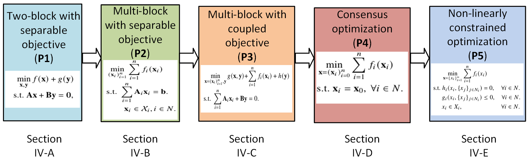
Figure 3: The roadmap of Section IV.

Throughout the section, we use $\mathcal{L}_{\rho}(\cdot)$ to denote an AL function with penalty parameter $\rho>0$ for a concerned problem. We assume that the AL functions can be easily derived from the context and thus do not discuss them in details. To be noted, in the algorithmic implementation of ADMM or its variants, we often only indicate the related arguments in subproblems for simplification. Without specifications, we use $\mathbf{x},\mathbf{y},\mathbf{x}_{i}$ to denote the primal variables, $\bm{\lambda},\bm{\lambda}_{i}$ to represent Lagrangian multipliers and $r,s,\tau$ to indicate dual stepsizes.

IV-A Two-block with separable objective

In this part, we focus on the standard two-block problem ($\mathbf{P1}$). In addition to classical ADMM, a number of ADMM variants have been developed either for different situations or with different features. These ADMM variants range from symmetric ADMM, fast ADMM, generalized ADMM, linearized ADMM and stochastic ADMM. They all can be viewed as the extension of classical ADMM with the integration of certain techniques (i.e., symmetric primal-dual scheme, Nesterov acceleration, proximal regularization and linearization). Compared with classical ADMM, these ADMM variants are often celebrated by their distinguishing features, such as improved convergence rate, easier subproblems, low per-iteration complexity and compatible with uncertain information. An overview of the relationships and features of the ADMM variants for solving two-block problem ($\mathbf{P1}$) is shown in Fig. 4. We distinguish the convex and nonconvex methods by solid and dashed boxes. In the sequel, we introduce each of those methods.

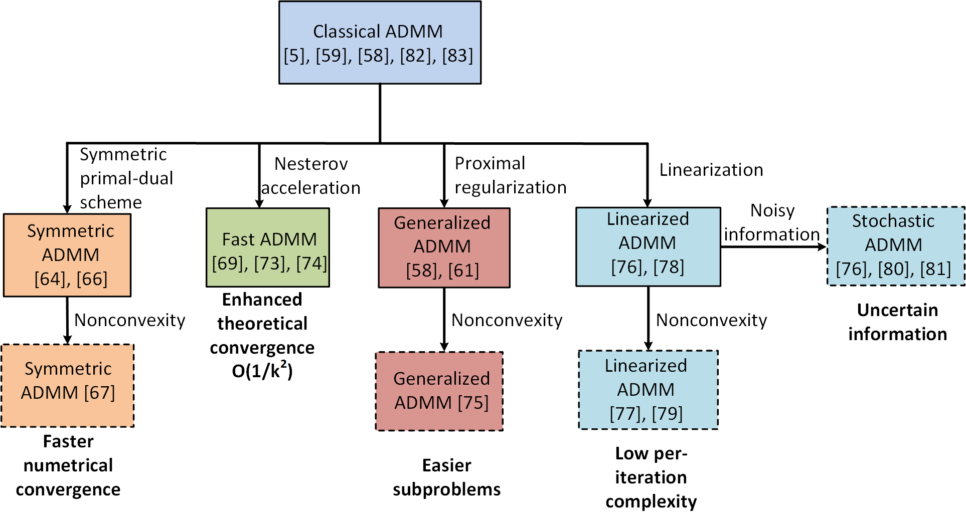
Figure 4: An overview of ADMM variants for solving two-block problem ($\mathbf{P1}$) (solid and dashed boxes indicate convex and nonconvex methods respectively).

IV-A1 Symmetric ADMM

As a well-known ADMM variant, the main alternation of symmetric ADMM over classical ADMM is that primal and dual variables are treated in a symmetric manner. Specifically, a dual update follows each block of primal update. The method takes the iterative scheme

Symmetric ADMM:

$$\textbf{Primal update:}~{}\mathbf{x}^{k+1}=\arg\min_{\mathbf{x}}\mathcal{L}_{\rho}(\mathbf{x},\mathbf{y}^{k},\bm{\lambda}^{k})$$

$$\textbf{Dual update:}~{}~{}~{}\bm{\lambda}^{k+\frac{1}{2}}=\lambda^{k}+r\rho(\mathbf{A}\mathbf{x}^{k+1}+\mathbf{B}\mathbf{y}^{k})$$

$$\textbf{Primal update:}~{}\mathbf{y}^{k+1}=\arg\min_{\mathbf{y}}\mathcal{L}_{\rho}(\mathbf{x}^{k+1},\mathbf{y},\bm{\lambda}^{k})$$

$$\textbf{Dual update:}~{}~{}~{}\bm{\lambda}^{k+1}=\bm{\lambda}^{k+\frac{1}{2}}+s\rho(\mathbf{A}\mathbf{x}^{k+1}+\mathbf{B}\mathbf{y}^{k+1})$$

Symmetric ADMM was developed simultaneously as classical ADMM by Glowinski in the 1970s [62]. The method was primary termed ALG3 until its equivalence to Peaceman-Rachford splitting method (PRSM) was discovered for trivial dual stepsizes $r=1$ and $s=1$ [50, 51, 63]. Note that symmetric ADMM degenerates into classical ADMM when the dual stepsize is set as $r=0$. The benefit of symmetric ADMM over classical ADMM is that it often yields faster convergence when convergent (see [64, 65] for some numerical examples).

We often see the trivial stepsizes $r=1$ and $s=1$ with symmetric ADMM, however they do not guarantee the convergence of the method for convex optimization as classical ADMM (see [65] for some divergent examples). This is because the generated sequence is not strictly contractive [65]. To fix such issue, a strictly contractive symmetric ADMM with damping dual stepsizes $r<1$ and $s<1$ was proposed in [65]. Besides, the ergodic convergence rate $\mathcal{O}(1/k)$ and non-ergodic convergence rate $\mathcal{O}(1/k)$ were established. Further, it was argued that the damping stepsizes $r<1$ and $s<1$ are not greeted and one normally prefers larger dual stepsizes to achieve faster convergence [66]. To deal with such a contradiction, [66] comprehensively studied the dual stepsize $(r,s)$ to ensure the convergence of symmetirc ADMM and identified the admissible domain $\mathcal{D}=\{(s,r)|s\in(0,\frac{\sqrt{5}+1}{2}),r\in(-1,1),r+s>0,|r|<1+s-s^{2}\}$. This implies that the dual stepsizes of symmertic ADMM are actually not restricted to $r<$ and $s<1$. Moreover, the admissible domain $\mathcal{D}$ actually has enlarged the Fortin and Glowinski constant $\tau\in(0,\frac{\sqrt{5}+1}{2})$ with classical ADMM, which infers that symmetric ADMM enjoys larger flexibility in parameter settings over classical ADMM.

The above results are for convex optimization. Symmetric ADMM has already been generalized to nonconvex counterparts (i.e., $f$ and $g$ are nonconvex). Specifically, [67] established the convergence of the method in nonconvex setting under the conditions: i) $g$ is $\operatorname{\text{Lipschitz}}$ differentiable, and ii) ${\rm Im}(\mathbf{A})\subseteq{\rm Im}(\mathbf{B})$, and the mapping $p(u)=\{\arg\min_{\mathbf{y}}g(\mathbf{y}):\mathbf{B}\mathbf{y}=u\}$ is $\operatorname{\text{Lipschitz}}$ smooth. Actually, condition ii) is a weaker assumption of full column rank $\mathbf{B}$ [68]. The faster convergence behaviors of symmetric ADMM over classical ADMM have been corroborated by many numerical studies [67].

IV-A2 Fast ADMM

As discussed, classical ADMM and symmetric ADMM only promise an $\mathcal{O}(1/k)$ convergence rate. To enhance the convergence rate, [69] proposed an accelerated ADMM variant by combining classical ADMM with Nesterov acceleration technique. This leads to a fast ADMM that ensures an $\mathcal{O}(1/k^{2})$ convergence rate for a class of strongly convex problems (i.e., $f$ and $g$ are strongly convex, $g$ is convex quadratic). The Nesterov acceleration technique was originally developed for unconstrained smooth convex optimization [70]. This technique is attractive for it can improve the convergence rate of first-order gradient methods by an order, i.e., from $\mathcal{O}(1/k)$ to $\mathcal{O}(1/k^{2})$, which is argued to be the best attainable computation efficiency with first-order information. This technique was later extended to a proximal gradient method for unconstrained nonsmooth and nonconvex optimization, which has enjoyed wide success in the domain of machine learning [71, 71, 72]. Central to Nesterov acceleration is to introduce an interpolation step in terms of the current and preceding iterates at each iteration. The combination of Nesterov acceleration with classical ADMM is reasonable as ADMM can be seen as a first-order solver of ALM. The implementation of fast ADMM is presented below.

Fast ADMM:

$$\textbf{Primal update:}~{}\begin{cases}&\!\!\!\mathbf{x}^{k}=\arg\min_{\mathbf{x}}\mathcal{L}_{\rho}(\mathbf{x},\hat{\mathbf{y}}^{k},\hat{\bm{\lambda}}^{k})\\ &\!\!\!\mathbf{y}^{k}=\arg\min_{\mathbf{y}}\mathcal{L}_{\rho}(\mathbf{x}^{k},\mathbf{y},\hat{\bm{\lambda}}^{k})\\ \end{cases}$$

$$\textbf{Dual update:}~{}~{}~{}~{}\bm{\lambda}^{k}=\hat{\bm{\lambda}}^{k}+\rho(\mathbf{A}\mathbf{x}^{k}+\mathbf{B}\mathbf{y}^{k})$$

$$\textbf{Nesterov stepsize:}~{}a_{k+1}=\frac{1+\sqrt{1+4a_{k}^{2}}}{2}$$

$$\textbf{Interpolation step:}\begin{cases}\hat{\mathbf{x}}^{k+1}=\mathbf{x}^{k}+\frac{a_{k}-1}{a_{k+1}}(\mathbf{x}^{k}-\mathbf{x}^{k-1})\\ \hat{\mathbf{y}}^{k+1}=\mathbf{y}^{k}+\frac{a_{k}-1}{a_{k+1}}(\mathbf{y}^{k}-\mathbf{y}^{k-1})\\ \hat{\bm{\lambda}}^{k+1}=\bm{\lambda}^{k}+\frac{a_{k}-1}{a_{k+1}}(\bm{\lambda}^{k}-\bm{\lambda}^{k-1})\\ \end{cases}$$

where $\{a_{k}\}_{k=1}^{K}$ represents the interpolation stepsize of Nesterov acceleration. Note that the main alternation of fast ADMM over classical ADMM is that an interpolation procedure is introduced to moderate the current and preceding primal-dual updates $(\mathbf{x}^{k},\mathbf{y}^{k},\bm{\lambda}^{k})$ and $(\mathbf{x}^{k-1},\mathbf{y}^{k-1},\bm{\lambda}^{k-1})$ generated by classical ADMM at the end of each iteration. This leads to the modified primal-dual updates $(\hat{\mathbf{x}}^{k},\hat{\mathbf{y}}^{k},\hat{\bm{\lambda}}^{k})$ that serve the next update. The work [69] established the $\mathcal{O}(1/k^{2})$ convergence rare of fast ADMM for the special case where $f,g$ are both strongly convex and $g$ is besides quadratic. However, for more general problems, the theoretical results are still open questions.

The difficulty to establish the convergence of fast ADMM for general problems lies in the fact that classical ADMM is actually not a first-order descent solver for ALM like gradient-based methods. In other words, we do not have the monotonically decreasing property of the objective value w.r.t. the iterations with ADMM. This can be perceived from the perspective of DRSM considering their equivalence [73]. However, it was argued that a descent solver may be constructed by adding some monitoring and correction steps (see [74] for an example). This actually sheds some lights on the generalization of fast ADMM to more general problems.

IV-A3 Generalized ADMM

Note that the main computation burden with classical ADMM lies in solving the subproblems iteratively. Therefore, it is significant to enable easier subproblems to improve computation efficiency. To achieve such a goal, generalized ADMM was proposed as an advanced version of classical ADMM [61, 58, 75]. The main idea is to optimize some proximal surrogates of the subproblems which are often much easier than the original subproblems. Generalized ADMM takes the iterative scheme

Generalized ADMM:

Primal update:

$$\!\!\!\!\begin{cases}&\!\!\!\mathbf{x}^{k+1}=\arg\min_{\mathbf{x}}\mathcal{L}_{\rho}(\mathbf{x},\mathbf{y}^{k},\bm{\lambda}^{k})+\frac{1}{2}\|\mathbf{x}-\mathbf{x}^{k}\|^{2}_{\mathbf{P}}\\ &\!\!\!\mathbf{y}^{k+1}=\arg\min_{\mathbf{y}}\mathcal{L}_{\rho}(\mathbf{x}^{k+1},\mathbf{y},\bm{\lambda}^{k})+\frac{1}{2}\|\mathbf{y}-\mathbf{y}^{k}\|^{2}_{\mathbf{Q}}\\ \end{cases}$$

$$\textbf{Dual update:}~{}~{}\bm{\lambda}^{k+1}=\bm{\lambda}^{k}+\tau\rho(\mathbf{A}\mathbf{x}^{k+1}+\mathbf{B}\mathbf{y}^{k+1})$$

where $\mathbf{P}\in\mathbf{R}^{n\times n}$ and $\mathbf{Q}\in\mathbf{R}^{n\times n}$ are symmetric positive semidefinite matrices. Note that the main alternations of generalized ADMM over classical ADMM are the proximal terms $\frac{1}{2}\|\mathbf{x}-\mathbf{x}^{k}\|^{2}_{\mathbf{P}}$ and $\frac{1}{2}\|\mathbf{y}-\mathbf{y}^{k}\|^{2}_{\mathbf{Q}}$ added to the subproblems of primal update. The method is termed generalized ADMM because it involves classical ADMM as a special case with zero $\mathbf{P}$ and $\mathbf{Q}$. The proximal terms are valuable for they bring benefits to the flexible implementation of the method. Specifically, some potential structures of $f$ and $g$ can be exploited to yield easier subproblems. For example, if $f$ is separable across its coordinates, we can select $\mathbf{P}=\tau\mathbf{I}-\rho\mathbf{A}^{\top}\mathbf{A}$ to yield an $\mathbf{x}$-subproblem

$$\mathbf{x}^{k+1}\!=\!\arg\min_{\mathbf{x}}f(\mathbf{x})\!+\!h(\mathbf{x}^{k})^{\top}(\mathbf{x}-\mathbf{x}^{k})\!+\!\frac{\tau}{2}\|\mathbf{x}-\mathbf{x}^{k}\|^{2}$$ (3)

where we have $h(\mathbf{x}^{k})=\mathbf{A}^{\top}\bm{\lambda}^{k}+\rho\mathbf{A}^{\top}(\mathbf{A}\mathbf{x}^{k}+\mathbf{B}\mathbf{y}^{k})$ and the $\mathbf{x}$-subproblem (3) reduces to a number of one-dimensional subproblems. Else if $f$ has easily computable proximal mapping, it is also beneficial because (3) is exactly the proximal mapping of $f$, i.e., $\mathbf{x}^{k+1}=\arg\min_{\mathbf{x}}f(\mathbf{x})+\frac{\tau}{2}\|\mathbf{x}-(\mathbf{x}^{k}-\tau^{-1}h(\mathbf{x}^{k}))\|^{2}$. Consider another case that $f$ is quadratic with Hessian matrix $\mathbf{H}_{f}$ (this implies that $f$ can be expressed by $f(\mathbf{x})=f(\mathbf{x}^{k})+\nabla f(\mathbf{x}^{k})^{\top}(\mathbf{x}-\mathbf{x}^{k})+\frac{1}{2}(\mathbf{x}-\mathbf{x}^{k})^{\top}\mathbf{H}_{f}(\mathbf{x}-\mathbf{x}^{k})$), we could select $\mathbf{P}=\tau\mathbf{I}-\rho\mathbf{A}^{\top}\mathbf{A}-\mathbf{H}_{f}$ to yield an $\mathbf{x}$-subproblem

$$\mathbf{x}^{k+1}=\arg\min_{\mathbf{x}}l(\mathbf{x}^{k})^{\top}(\mathbf{x}-\mathbf{x}^{k})+\frac{\tau}{2}\|\mathbf{x}-\mathbf{x}^{k}\|^{2}$$ (4)

where we have $l(\mathbf{x}^{k})=\nabla f(\mathbf{x}^{k})+\mathbf{A}^{\top}\bm{\lambda}^{k}+\rho\mathbf{A}^{\top}(\mathbf{A}\mathbf{x}^{k}+\mathbf{B}\mathbf{y}^{k})$. Note that (4) admits a gradient-like closed-form solution $\mathbf{x}^{k+1}=\mathbf{x}^{k}-\tau^{-1}l(\mathbf{x}^{k})$ and enjoys low per-iteration complexity. These are examples how generalized ADMM can make use of the proximal terms to yield easier subproblems. To be noted, the proximal terms with positive semidefinite $\mathbf{P}$ and $\mathbf{Q}$ will not disrupt the convergence property of classical ADMM. In other words, we do not require extra assumptions besides convexity to ensure the convergence of generalized ADMM. This can be understood that the proximal terms actually play the role of slowing down moving and enhancing convergence since they penalize the deviations from preceding updates. The $\mathcal{O}(1/k)$ iteration complexity of generalized ADMM was established for general convex optimization in [58]. For the special case where $f$ and $g$ are strongly convex and $\operatorname{\text{Lipschitz}}$ differentiable, the matrices $\mathbf{A},\mathbf{B}$ satisfy certain full row or column rank conditions, a global linear convergence rate was established in [61].

The above results are for convex optimization. For the nonconvex counterpart (i.e., $f$ and $g$ are nonconvex), the convergence of generalized ADMM towards stationary points was established under the conditions: i) $g$ is $\operatorname{\text{Lipschitz}}$ differentiable, and ii) $\mathbf{B}$ has full row rank [75]. Similar to the convex counterpart, the proximal terms play the role of yielding easier subproblems and will not disrupt convergence.

IV-A4 Linearized ADMM

Note that the implementations of above ADMM variants assume that the subproblems of primal update are easy to be solved exactly. There exist cases that the objective functions $f$ and $g$ are complex and solving the subproblems exactly is expensive or not desirable due to the high computation complexity. In such context, it is critical to figure out how to mitigate per-iteration complexity. To address such an issue, linearized ADMM was proposed with the idea of optimizing local linear approximations of subproblems, which often leads to some cheap gradient iterates in place of solving the subproblems exactly [76, 77]. The implementation of linearized ADMM takes the usual form of

Linearized ADMM:

$$\textbf{Primal update:}~{}\mathbf{x}^{k+1}=\big{[}\mathbf{x}^{k}-\alpha_{k}\nabla_{\mathbf{x}}\tilde{\mathcal{L}}_{\rho}(\mathbf{x}^{k},\mathbf{y}^{k},\bm{\lambda}^{k})\big{]}_{\mathbf{\mathcal{X}}}$$

$$\quad\quad\quad\quad\quad\quad\quad\mathbf{y}^{k+1}=\big{[}\mathbf{y}^{k}-\beta_{k}\nabla_{\mathbf{y}}\tilde{\mathcal{L}}_{\rho}(\mathbf{x}^{k+1},\mathbf{y}^{k},\bm{\lambda}^{k})\big{]}_{\mathbf{\mathcal{Y}}}$$

$$\textbf{Dual update:}~{}~{}~{}\bm{\lambda}^{k+1}=\bm{\lambda}^{k}+\rho(\mathbf{A}\mathbf{x}^{k+1}+\mathbf{B}\mathbf{y}^{k+1})$$

where $\tilde{\mathcal{L}}_{\rho}(\mathbf{x},\mathbf{y},\bm{\lambda})=\tilde{f}(\mathbf{x})+\tilde{g}(\mathbf{y})+\langle\bm{\lambda},\mathbf{A}\mathbf{x}+\mathbf{B}\mathbf{y}\rangle+\frac{\rho}{2}\|\mathbf{A}\mathbf{x}+\mathbf{B}\mathbf{y}\|^{2}$ aggregates the differentiable parts of AL function; $\nabla_{\mathbf{x}}\tilde{\mathcal{L}}_{\rho}(\mathbf{x},\mathbf{y},\bm{\lambda})$ and $\nabla_{\mathbf{y}}\tilde{\mathcal{L}}_{\rho}(\mathbf{x},\mathbf{y},\bm{\lambda})$ denote the gradients of $\tilde{\mathcal{L}}_{\rho}(\mathbf{x},\mathbf{y},\bm{\lambda})$ w.r.t. $\mathbf{x}$ and $\mathbf{y}$; the subsets $\mathbf{\mathcal{X}}$ and $\mathbf{\mathcal{Y}}$ indicate the local constraints related to decision variable $\mathbf{x}$ and $\mathbf{y}$. As clarified in problem ($\mathbf{P1}$), we have $f(\mathbf{x})=\tilde{f}(\mathbf{x})+I_{\mathbf{\mathcal{X}}}(\mathbf{x})$ and $g(\mathbf{y})=\tilde{g}(\mathbf{y})+I_{\mathbf{\mathcal{Y}}}(\mathbf{y})$. Note that the primal update of linearized ADMM reduces to two projected gradient iterates. They are actually derived from the proximal linearized subproblems

$$\mathbf{x}^{k+1}\!=\!\arg\min_{\mathbf{x}\in\mathbf{\mathcal{X}}}\langle\nabla_{\mathbf{x}}\tilde{\mathcal{L}}_{\rho}(\mathbf{x}^{k},\mathbf{y}^{k},\bm{\lambda}^{k}),\mathbf{x}-\mathbf{x}^{k}\rangle\!+\!\frac{1}{2\alpha_{k}}\|\mathbf{x}-\mathbf{x}^{k}\|^{2}$$

$$\mathbf{y}^{k+1}\!=\!\arg\min_{\mathbf{y}\in\mathbf{\mathcal{Y}}}\langle\nabla_{\mathbf{y}}\tilde{\mathcal{L}}_{\rho}(\mathbf{x}^{k+1},\mathbf{y}^{k},\bm{\lambda}^{k}),\mathbf{y}-\mathbf{y}^{k}\rangle\!+\!\frac{1}{2\beta_{k}}\|\mathbf{y}-\mathbf{y}^{k}\|^{2}$$

To be noted, the differentiable AL function $\tilde{\mathcal{L}}_{\rho}(\mathbf{x},\mathbf{y},\bm{\lambda})$ is linearized at $(\mathbf{x}^{k},\mathbf{y}^{k},\bm{\lambda}^{k})$ and $(\mathbf{x}^{k+1},\mathbf{y}^{k},\bm{\lambda}^{k})$ w.r.t. $\mathbf{x}$ and $\mathbf{y}$, and besides some proximal terms $\frac{1}{2\alpha_{k}}\|\mathbf{x}-\mathbf{x}^{k}\|^{2}$ and $\frac{1}{2\beta_{k}}\|\mathbf{y}-\mathbf{y}^{k}\|^{2}$ are added in the subproblems to control the accuracy of local linear approximation.

Linearized ADMM applies to both convex [76, 78] and nonconvex optimization [77, 79] but rests on different conditions to ensure convergence. One common condition is that the differentiable objective components $\tilde{f}$ and $\tilde{g}$ are $\operatorname{\text{Lipschitz}}$ differentiable. This can be understood that the $\operatorname{\text{Lipschitz}}$ differentiable property makes it possible to bound the linear approximation discrepancy by $|\tilde{f}(\mathbf{x})-\tilde{f}(\mathbf{x}^{k})-\langle\nabla\tilde{f}(\mathbf{x}^{k}),\mathbf{x}-\mathbf{x}^{k}\rangle|\leq\frac{L_{\tilde{f}}}{2}\|\mathbf{x}-\mathbf{x}^{k}\|^{2}$ where we assume $\tilde{f}$ $L_{\tilde{f}}$-$\operatorname{\text{Lipschitz}}$ differentiable. For convex optimization, the convergence and $\mathcal{O}(1/k)$ ergodic convergence rate of linearized ADMM were established in [76, 78]. For nonconvex counterpart, the convergence of linearized ADMM was established under slightly different conditions in [77] and [79]. Specifically, [77] assumed that $f$ and $g$ are $\operatorname{\text{Lipschitz}}$ differentiable (i.e., $\mathbf{\mathcal{X}},\mathbf{\mathcal{Y}}\subseteq\mathbf{R}^{n}$), and [79] made the assumptions that $g$ is $\operatorname{\text{Lipschitz}}$ differentiable (i.e., $\mathbf{\mathcal{Y}}\in\mathbf{R}^{n}$), ${\rm Im}(\mathbf{A})\subseteq{\rm Im}(\mathbf{B})$ and $\mathbf{B}$ has full column rank. Actually, these two works rely on the same key step to draw convergence, i.e., identifying a sufficiently decreasing and lower bounded Lyapunov function. To this end, they both require to bound the Lagrangian multipliers updates $\|\bm{\lambda}^{k+1}-\bm{\lambda}^{k}\|^{2}$ by the primal updates $\|\mathbf{x}^{k+1}-\mathbf{x}^{k}\|^{2}$ and $\|\mathbf{y}^{k+1}-\mathbf{y}^{k}\|^{2}$. Though the assumptions of there two works are different, they are actually used to achieve such same objective.

To be clarified, we only require that the objective functions to be linearized are $\operatorname{\text{Lipschitz}}$ differentiable both in convex and nonconvex optimization. The method can be adapted to the case where only one objective function is $\operatorname{\text{Lipschitz}}$ differentiable. In such case, we can only linearize the subproblem with $\operatorname{\text{Lipschitz}}$ differentiable objective and solve the other one exactly. The established theoretical results still hold.

IV-A5 Stochastic ADMM

Another branch of extension of ADMM is to account for the incomplete and inaccurate information in practical implementation. A typical scenario is that explicit formulas of objective functions are not available for a complex engineering system and instead only noisy gradients regarding the system performance (i.e., the gradients of objective functions) are accessible by means of sampling. In such situation, it is impossible to solve the subproblems with classical ADMM or its variants exactly. Therefore, [76, 80, 81] studied a stochastic version of ADMM. The basic idea is to perform some gradient-like iterates with the available noisy gradients at each iteration in place of solving the subproblems comprehensively. The idea is natural since only gradient information is accessible in such situation. Stochastic ADMM takes the iterative scheme

Stochastic ADMM:

$$\textbf{Primal update:}~{}\mathbf{x}_{k+1}=\big{[}\mathbf{x}^{k}-\alpha_{k}\nabla_{\mathbf{x}}\tilde{\mathcal{L}}_{\rho}(\mathbf{x}^{k},\mathbf{y}^{k},\bm{\lambda}^{k},\xi^{k+1})\big{]}_{\mathbf{\mathcal{X}}}$$

$$\quad\quad\quad\quad\quad\quad\quad\mathbf{y}^{k+1}=\!\big{[}\mathbf{y}^{k}-\beta_{k}\nabla_{\mathbf{y}}\tilde{\mathcal{L}}_{\rho}(\mathbf{x}^{k+1},\mathbf{y}^{k},\bm{\lambda}^{k},\zeta^{k+1})\big{]}_{\mathbf{\mathcal{Y}}}$$

$$\textbf{Dual update:}~{}~{}~{}\bm{\lambda}^{k+1}=\bm{\lambda}^{k}+\rho(\mathbf{A}\mathbf{x}^{k+1}+\mathbf{B}\mathbf{y}^{k+1})$$

One may note that stochastic ADMM resembles linearized ADMM. The only difference lies in the gradients used to perform the primal update. Specifically, stochastic ADMM uses some noisy gradients of AL function to perform the primal update whereas linearized ADMM uses deterministic and accurate ones. We have $\xi^{k+1}$ and $\zeta^{k+1}$ characterize the estimation errors of gradients for the objective functions $\tilde{f}$ and $\tilde{g}$ at iteration $k$, which can be expressed by $\nabla\tilde{f}(\mathbf{x}^{k},\xi^{k+1})$ and $\nabla\tilde{g}(\mathbf{y}^{k},\!\zeta^{k+1})$ and the corresponding noisy gradients of AL function are $\nabla_{\mathbf{x}}\tilde{\mathcal{L}}_{\rho}(\mathbf{x}^{k},\mathbf{y}^{k},\bm{\lambda}^{k},\xi^{k+1})$ and $\nabla_{\mathbf{y}}\tilde{\mathcal{L}}_{\rho}(\mathbf{x}^{k+1},\!\mathbf{y}^{k},\!\bm{\lambda}^{k},\zeta^{k\!+1})$.

Clearly, the convergence of stochastic ADMM depends on the accuracy of the estimations of gradients. For the usual case that the estimations are unbiased and variance-bounded, [76, 80, 81] established the convergence of the method for convex optimization with $\operatorname{\text{Lipschitz}}$ differentiable objective functions $\tilde{f}$ and $\tilde{g}$. Despite the similarity of stochastic ADMM to linearized ADMM, they actually show quite different convergence behaviors due to the inaccurate and accurate information used in the iterative process. Specifically, the convergence of linearized ADMM can be directly examined in a deterministic sense, whereas that can only be evaluated in a stochastic space by studying the expectation of performance metrics with stochastic ADMM. Moreover, due to the inaccurate information, stochastic ADMM only promises $\mathcal{O}(1/\sqrt{k})$ convergence rate in contrast to the $\mathcal{O}(1/k)$ convergence rate of linearized ADMM with accurate information [76, 80, 81]. For the special case where $\tilde{f}$ and $\tilde{g}$ are strongly convex and $\operatorname{\text{Lipschitz}}$ differentiable, stochastic ADMM ensures an $\mathcal{O}(\frac{\log k}{k})$ ergodic convergence rate [80, 81].

Similar to linearized ADMM, stochastic ADMM also applies to the special case where only one objective function is $\operatorname{\text{Lipschitz}}$ differentiable. In such context, the method can be applied if the other subproblem has explicitly available objective function and can be solved exactly in the iterative process.

TABLE II: ADMM variants for solving two-block optimization ($\mathbf{P1}$)

Methods	Main assumptions	Types	Convergence	Features	References
Classic ADMM	$f$ and $g$ convex. Existence of saddle points.	Gauss-Seidel	Global convergence. Global optima. Convergence rate $\mathcal{O}(1/k)$ (convex). Linear convergence (strongly convex)	Convex.	[5, 59] [58, 82, 83]
Symmetric ADMM	$f$ and $g$ convex. $(r,s)$ properly selected. Existence of saddle points.	Gauss-Seidel	Global convergence. Global optima. Convergence rate $\mathcal{O}(1/k)$.	Faster numerical convergence. Convex.	[64, 66]
	$f$ and $g$ nonconvex. $g$ $\operatorname{\text{Lipschitz}}$ differentiable. ${\rm Im}(\mathbf{A})\subseteq{\rm Im}(\mathbf{B})$. $\mathbf{B}$ full column rank.	Gauss-Seidel	Global convergence. Stationary points.	Faster numerical convergence. Nonconvex.	[67]
Fast ADMM	$f$ and $g$ convex. $g$ convex quadratic. Existence of saddle points.	Gauss-Seidel	Global convergence. Convergence rate $\mathcal{O}(1/k^{2})$.	Enhanced convergence rate. Convex.	[69, 74, 73]
Generalized ADMM	$f$ and $g$ convex. Existence of saddle points.	Gauss-Seidel	Global convergence. Global optima. Convergence rate $\mathcal{O}(1/k)$ (convex). Linear convergence (strongly convex).	Easy subproblems. Convex.	[61, 58]
	$\mathbf{B}$ has full row rank. $g$ $\operatorname{\text{Lipschitz}}$ differentiable.	Gauss-Seidel	Global convergence. Global optima. Linear convergence.	Easy subproblems Nonconvex	[75]
Linearized ADMM	$f$ and $g$ convex $f$ and $g$ $\operatorname{\text{Lipschitz}}$ differentiable.	Gauss-Seidel	Global convergence. Global optima. Convergence rate $\mathcal{O}(1/k)$.	Low per-iteration complexity. Convex.	[76, 78]
	$f$ and $g$ $\operatorname{\text{Lipschitz}}$ differentiable. ${\rm Im}(\mathbf{A})\subseteq{\rm Im}(\mathbf{B})$. $\mathbf{B}$ full column rank.	Gauss-Seidel	Stationary. Linear convergence.	Low per-iteration complexity. Nonconvex.	[77, 79]
Stochastic ADMM	$f$ and $g$ convex. $f$ and $g$ $\operatorname{\text{Lipschitz}}$ differentiable.	Gauss-Seidel	Global convergence. Global optima under expectation. Convergence rate $\mathcal{O}(1/\sqrt{k})$ (convex). Convergence rate $\mathcal{O}(\log k/k)$ (strongly convex).	Incomplete and inaccurate information. Convex.	[76, 80, 81]

Summary: In this part, we reviewed ADMM variants for solving the linearly constrained two-block problem ($\mathbf{P1}$). In addition to classic ADMM that has been recognized as a benchmark, a number of variants are now available either with distinguishing features or suitable for different situations. We report the ADMM variants (including classical ADMM) in terms of main assumptions, decomposition schemes (i.e., type), convergence properties, main features and references in TABLE II. We have the following main conclusions. ADMM and its variants provide sublinear convergence (i.e., $\mathcal{O}(1/k)$, $\mathcal{O}(1/k^{2})$) for general convex optimization. For the special case where the objective functions are strongly convex and $\operatorname{\text{Lipschitz}}$ differentiable, linear convergence can be achieved (see classical ADMM, generalized ADMM and linearized ADMM). Some of the ADMM variants have been generalized to nonconvex optimization but require certain $\operatorname{\text{Lipschitz}}$ differentiable properties of the objective functions and rank conditions on the coefficient matrices $\mathbf{A},\mathbf{B}$ (see symmetric ADMM, generalized ADMM and linearized ADMM). These ADMM variants can be celebrated by their distinguishing features, such as faster numerical convergence (symmetric ADMM), enhanced convergence rate (fast ADMM), easier subproblems (generalized ADMM), low per-iteration complexity (linearized ADMM) and compatible with inaccurate information (stochastic ADMM).

IV-B Multi-block with separable objective

Previously, we have focused on two-block optimization and assumed two computing agents to undertake the computation. It is more than often that we have a multi-agent system and the computation is expected to be distributed across multiple agents. This usually corresponds to a constrained multi-block optimization where the objective is the sum of objectives of individual agents. This class of problems takes the general formulation of

$$\min_{(\mathbf{x}_{i})_{i=1}^{n}}\sum_{i=1}^{n}f_{i}(\mathbf{x}_{i}) \mathbf{P}2$$ ()

$${\rm s.t.}~{}\sum_{i=1}^{n}\mathbf{A}_{i}\mathbf{x}_{i}=\mathbf{b}.$$

$$\quad\quad\mathbf{x}_{i}\in\mathbf{\mathcal{X}}_{i},i\in N.$$

where $f_{i}:\mathbf{R}^{n_{i}}\rightarrow\mathbf{R}$ are given objective functions of the agents defined on their decision variables $\mathbf{x}_{i}\in\mathbf{R}^{n_{i}},i\in N$; $\mathbf{\mathcal{X}}_{i}\in\mathbf{R}^{n_{i}}$ are local bounded convex constraints imposed on decision variables $\mathbf{x}_{i},i\in N$; $\mathbf{A}_{i}\in\mathbf{R}^{l\times n_{i}}$ and $\mathbf{b}\in\mathbf{R}^{l}$ are coefficient matrices that encode the linear couplings across the agents. Problem ($\mathbf{P}2$) can be viewed as an extension of ($\mathbf{P1}$), allowing arbitrary number of decision blocks instead of only two. By defining $\mathbf{x}:=(\mathbf{x}_{i})_{i=1}^{n}$ and $\mathbf{A}:=(\mathbf{A}_{i})_{i=1}^{n}$, we have the linear couplings take the compact format $\mathbf{A}\mathbf{x}=\mathbf{b}$. In ($\mathbf{P}2$), we explicitly indicate the local bounded convex constraints $\mathbf{\mathcal{X}}_{i}$ to show that the problem is entirely nonsmooth w.r.t. each decision block. This is an important problem characteristic to be considered while designing an ADMM variant for distributed optimization.

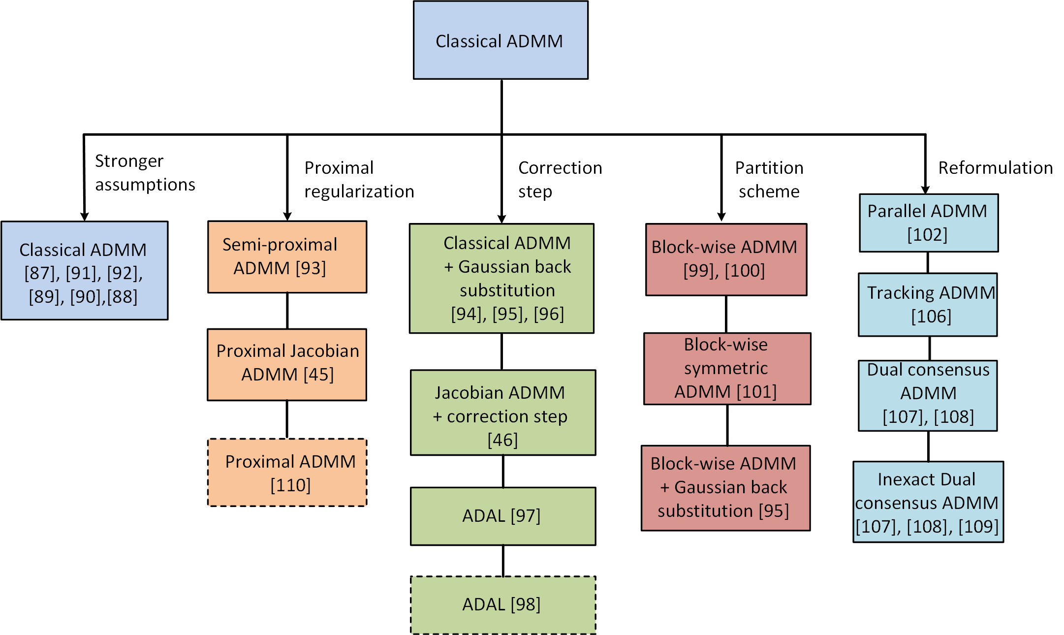
Figure 5: An overview of ADMM variants resulting from the different modifications of classical ADMM for solving multi-block problem ($\mathbf{P}2$) (solid and dashed boxes indicate convex and nonconvex methods respectively).

In this part, we survey ADMM and its variants for solving problem ($\mathbf{P}2$) both in convex and nonconvex settings. Since ($\mathbf{P1}$) is a special case of ($\mathbf{P}2$) that involves only two decision blocks, the methods of this part are readily applicable to ($\mathbf{P1}$) provided that corresponding conditions are satisfied.

Basically, the direct extension of classical ADMM to multi-block problem ($\mathbf{P}2$) is not necessarily convergent and some modifications are required to ensure convergence [84]. In the literature, the modifications are diverse and range from imposing stronger assumptions, adding proximal regularization, adding some correction steps, leveraging partition schemes and properly reformulating problems. These modifications lead to a plentiful of ADMM variants for solving multi-block problem ($\mathbf{P}2$). An overview of the ADMM variants resulting from the different modifications of classical ADMM for solving multi-block problem ($\mathbf{P}2$) is shown in Fig. 5. We distinguish the convex and nonconvex methods by solid and dashed boxes respectively. These ADMM variants are often preferred for different features, such as fast convergence, parallel implementatio, flexible communication (i.e., networked communication) and low per-iteration complexity etc. In what follows, we introduce each of those methods.

IV-B1 Classic ADMM

The direct application of classical ADMM to multi-block problem ($\mathbf{P}2$) is natural and takes the following iterative scheme.

Classic ADMM:

$$\textbf{Primal update:}~{}~{}\mathbf{x}_{i}^{k+1}=\arg\min_{\mathbf{x}_{i}\in\mathbf{\mathcal{X}}_{i}}\mathcal{L}_{\rho}(\mathbf{x}_{<i}^{k+1},\mathbf{x}_{i},\mathbf{x}_{>i}^{k},\bm{\lambda}^{k}),i\in N.$$

$$\textbf{Dual update:}~{}~{}~{}\bm{\lambda}^{k+1}=\bm{\lambda}^{k}+\rho(\mathbf{A}\mathbf{x}^{k+1}-\mathbf{b}).$$

Despite the method has found many successful applications (see [85, 86] for examples), the convergence is not secured for general multi-block problem ($\mathbf{P}2$) (i.e., $n\geq 3$) in convex setting [84]. Many efforts have been made in studying the convergence conditions for the multi-block extensions [87, 88, 89, 90]. The results are diverse due to the different scenarios (i.e., different numbers of decision blocks) concerned and the different ways used to draw convergence. As an earlier work, [89] focused on the special case with $n=3$ blocks and established the convergence of the method under the conditions: i) $f_{2},f_{3}$ are strongly convex, and ii) $f_{1}$ strongly convex or $\mathbf{A}_{1}$ has full column rank. The results are specialized to $n=3$ blocks and can not be directly generalized to arbitrary $n$ blocks. Similarly for the 3-block case, [90] established the convergence of the method under slightly different conditions: i) $f_{1},f_{2}$ are convex and $f_{3}$ is strongly convex, and ii) $\mathbf{A}_{2}$ and $\mathbf{A}_{3}$ have full column rank. For general $n$-block case, [88] argued that the convergence can be guaranteed provided that all of the objective functions $f_{i}$ are strongly convex. Later, the conditions were relaxed to $n-1$ strongly convex objective functions in [91, 87, 92]. Overall, these conditions are sufficient instead of necessary conditions to guarantee the convergence of the method. Presently, there is no consensus on the necessary convergence conditions of classical ADMM for the multi-block extension.

IV-B2 Semi-proximal ADMM

While classic ADMM has focused on imposing stricter assumptions to ensure convergence in multi-block setting, another line of works has turned to modify the update scheme of classical ADMM. One example is semi-proximal ADMM that proposes to regularize the subproblems by some proximal terms [93]. The method takes the following iterative procedures.

Semi-proximal ADMM:

Primal update:

$$~{}~{}\mathbf{x}_{i}^{k+1}=\arg\min_{\mathbf{x}_{i}\in\mathbf{\mathcal{X}}_{i}}\mathcal{L}_{\rho}(\mathbf{x}_{<i}^{k+1},\mathbf{x}_{i},\mathbf{x}_{>i}^{k},\bm{\lambda}^{k})+\frac{1}{2}\|\mathbf{x}_{i}-\mathbf{x}_{i}^{k}\|^{2}_{\mathbf{P}_{i}},i\in N.$$

$$\textbf{Dual update:}~{}\bm{\lambda}^{k+1}=\bm{\lambda}_{k}+\tau\rho(\mathbf{A}\mathbf{x}^{k+1}-\mathbf{b})$$

where $\mathbf{P}_{i}\in\mathbf{R}^{n_{i}\times n_{i}}$ are positive semidefinite matrices. Note that the major modifications of semi-proximal ADMM over classical ADMM are the proximal terms $\frac{1}{2}\|\mathbf{x}_{i}-\mathbf{x}_{i}^{k}\|^{2}_{\mathbf{P}_{i}}$ added to the subproblems. The proximal terms were found to be able to enhance the convergence property of method and yield weaker convergence conditions than classical ADMM. Specifically for the $3$-block case, it only requires $f_{2}$ strongly convex with sufficiently large proximal coefficient matrices $\mathbf{P}_{i}$ [93]. In addition, it was proved that the method admits any nontrivial dual stepsizes $\tau\in(0,\frac{\sqrt{5}+1}{2})$. However, the results are limited to $n=3$ blocks and for general $n$-block case, the convergence conditions and theoretical convergence remain to be addressed.

IV-B3 Proximal Jacobian ADMM

Note that semi-proximal ADMM results from the combination of $\operatorname{Gauss-Seidel}$ decomposition with proximal regularization. A natural idea is to consider the combination of $\operatorname{Jacobian}$ decomposition and proximal regularization. This has led to the proximal Jacobian ADMM variant that takes the following iterative scheme [45].

Proximal Jacobian ADMM:

Primal update:

$$\quad\mathbf{x}_{i}^{k+1}=\arg\min_{\mathbf{x}_{i}\in\mathbf{\mathcal{X}}_{i}}\mathcal{L}_{\rho}(\mathbf{x}_{i},\mathbf{x}_{-i}^{k},\bm{\lambda}^{k})+\frac{1}{2}\|\mathbf{x}_{i}-\mathbf{x}_{i}^{k}\|^{2}_{\mathbf{P}_{i}},i\in N.$$

$$\textbf{Dual update:}~{}\bm{\lambda}^{k+1}=\bm{\lambda}^{k}+\tau\rho(\mathbf{A}\mathbf{x}^{k+1}-\mathbf{b})$$

The benefit of the $\operatorname{Jacobian}$ version is the parallelizable implementation. Since $\operatorname{Jacobian}$ decomposition also only provides an approximation to the joint primal update, some proximal terms $\frac{1}{2}\|\mathbf{x}_{i}-\mathbf{x}_{i}^{k}\|^{2}_{\mathbf{P}_{i}}$ are also required to control the $\operatorname{Jacobian}$ approximation accuracy. Clearly, the proximal regularization matrices $\mathbf{P}_{i}$ should be selected sufficiently large. It was proved that we require $\mathbf{P}_{i}>\rho(n-1)\mathbf{A}_{i}^{\top}\mathbf{A}_{i}$ (for the dual stepsize $\tau=1$) to ensure convergence of the method for general convex optimization [45]. Under such condition, the $o(1/k)$ convergence rate of the method was further established. From the results, we note that the proximal coefficient matrices are generally required to be linearly increased with the problem scale $n$. Since the proximal terms play the role of slowing down moving, slower convergence of the method is likely to be observed with larger-scale problems.

IV-B4 Classic ADMM + Gaussian back substitution

Though the direct extension of classical ADMM to multi-block problem ($\mathbf{P}2$) is not necessarily convergent, it was found that a convergent sequence can be constructed by properly twisting the generated sequences [94]. This leads to the idea of using classical ADMM to generate a sequence as a prediction and then using some correction steps to twist a convergent sequence. Following such idea, a number of prediction-correction ADMM variants have been developed. One of such methods is the classical ADMM + Gaussian back substitution proposed in [94, 95, 96]. The method takes the following iterative scheme.

Classic ADMM + Gaussian back substitution:

$$\textbf{Primal update:}~{}\tilde{\mathbf{x}}_{i}^{k}=\arg\min_{\mathbf{x}_{i}\in\mathbf{\mathcal{X}}_{i}}\mathcal{L}_{\rho}(\tilde{\mathbf{x}}_{<i}^{k},\mathbf{x}_{i},\mathbf{x}_{>i}^{k},\bm{\lambda}^{k}),\forall i\in N.$$

$$\textbf{Dual update:}~{}\tilde{\bm{\lambda}}^{k}=\bm{\lambda}^{k}+\rho(\mathbf{A}\tilde{\mathbf{x}}^{k}-\mathbf{b}).$$

$$\textbf{Gaussian back substitution}:\mathbf{P}(\mathbf{v}^{k+1}-\mathbf{v}^{k})=\alpha(\tilde{\mathbf{v}}^{k}-\mathbf{v}^{k})$$

where we have $\mathbf{P}=\mathbf{H}^{-1}\mathbf{M}^{\top}$ with

$$\mathbf{M}=\begin{pmatrix}\rho\mathbf{A}_{2}^{\top}\mathbf{A}_{2}&\bm{0}&\cdots&\cdots&\bm{0}\\ \rho\mathbf{A}_{3}^{\top}\mathbf{A}_{2}&\rho\mathbf{A}_{3}^{\top}\mathbf{A}_{3}&\cdots&\cdots&\bm{0}\\ \vdots&\vdots&\vdots&\vdots&\vdots\\ \rho\mathbf{A}_{n}^{\top}\mathbf{A}_{2}&\rho\mathbf{A}_{n}^{\top}\mathbf{A}_{3}&\cdots&\rho\mathbf{A}_{n}^{\top}\mathbf{A}_{n}&\bm{0}\\ \bm{0}&\bm{0}&\cdots&\bm{0}&\frac{1}{\rho}\mathbf{I}_{l}\\ \end{pmatrix}$$

$$\mathbf{H}={\rm diag}\big{(}\rho\mathbf{A}_{2}^{\top}\mathbf{A}_{2},\rho\mathbf{A}_{3}^{\top}\mathbf{A}_{3},\cdots,\rho\mathbf{A}_{n}^{\top}\mathbf{A}_{n},\frac{1}{\rho}\mathbf{I}_{l}\big{)}.$$

where $\mathbf{v}=(\mathbf{x}_{2}^{\top},\mathbf{x}_{3}^{\top},\cdots,\mathbf{x}_{N}^{\top},\bm{\lambda}^{\top})^{\top}$ stacks the primal and dual variables excluding $\mathbf{x}_{1}$; the scalar $\alpha$ is a correction stepsize. The first block $\mathbf{x}_{1}$ is excluded from the Gaussian back substitution (i.e., correction step) because $\mathbf{x}_{1}$ is an intermediate variable and does not join next iterates. Classic ADMM + Gaussian back substitution consists of two main steps: the first step uses classical ADMM to generate a prediction $\tilde{\mathbf{v}}^{k}$ and the second step uses Gaussian back substitution to correct the generated sequence and obtain a modified sequence $\mathbf{v}^{k+1}$ for serving the next update. Specifically, the predictions step are performed in a forward manner, i.e., $\tilde{\mathbf{x}}_{1}^{k}\rightarrow\tilde{\mathbf{x}}_{2}^{k}\rightarrow\cdots\rightarrow\tilde{\mathbf{x}}_{n}^{k}\rightarrow\tilde{\bm{\lambda}}^{k}$ and the correction steps are carried out in a backward fashion, i.e., $\bm{\lambda}^{k+1}\rightarrow\mathbf{x}_{n}^{k+1}\rightarrow\mathbf{x}_{n-1}^{k+1}\rightarrow\cdots\rightarrow\mathbf{x}_{2}^{k+1}$. The former results from the $\operatorname{Gauss-Seidel}$ scheme and the latter is induced from the upper triangle property of matrix $\mathbf{P}$ which is easy to infer from $\mathbf{H}$ and $\mathbf{M}$. The convergence and $\mathcal{O}(1/k)$ convergence rate in both ergodic and noner-godic sense together with the admissible correction stepsizes $\alpha\in(0,1)$ of the method were established for convex optimization in [94, 95, 96]. One may note that the Gaussian back substitution can be converted to $\mathbf{v}^{k+1}=\mathbf{v}^{k}-\alpha\mathbf{M}^{-\top}\mathbf{H}(\mathbf{v}^{k}-\tilde{\mathbf{v}}^{k})$, this is not necessary considering the upper triangle property of $\mathbf{P}$, which can be directly exploited to enable easy computation and avoid calculating the inverse and transpose matrix $\mathbf{M}^{-\top}$.

IV-B5 Jacobian ADMM + correction step

Jacobian ADMM + correction step is another typical prediction-correction ADMM variant for solving multi-block problem ($\mathbf{P}2$) [46]. The basic idea is to obtain a convergent sequence by twisting the sequence generated by a Jacobian ADMM. The method takes the following iterative procedures.

Jacobian ADMM + correction step:

$$\textbf{Primal update:}~{}~{}\tilde{\mathbf{x}}_{i}^{k}=\arg\min_{\mathbf{x}_{i}\in\mathcal{\mathbf{\mathcal{X}}}_{i}}\mathcal{L}_{\rho}(\mathbf{x}_{i},\mathbf{x}_{-i}^{k},\bm{\lambda}^{k}),\forall i\in N.$$

$$\textbf{Dual update:}~{}~{}\quad\tilde{\bm{\lambda}}^{k}=\bm{\lambda}^{k}+\rho(\mathbf{A}\tilde{\mathbf{x}}^{k}-\mathbf{b})$$

$$\textbf{Correction step:}~{}~{}\mathbf{w}^{k+1}=\mathbf{w}^{k}-\alpha(\mathbf{w}^{k}-\tilde{\mathbf{w}}^{k})$$

where $\mathbf{w}=(\mathbf{x}_{1}^{\top},\mathbf{x}_{2}^{\top},\cdots,\mathbf{x}_{N}^{\top},\bm{\lambda}^{\top})^{\top}$ stacks the primal and dual variables; the scalar $\alpha$ is a correction stepsize. Very similar to classical ADMM + Gaussian back substitution, this method is also composed of the prediction and correction steps. The major difference is that this method uses a $\operatorname{Jacobian}$ ADMM to generate a prediction $\tilde{\mathbf{w}}^{k}$ instead of the $\operatorname{Gauss-Seidel}$ counterpart. One may note that this brings difference to the correction steps where the first block $\mathbf{x}_{1}$ is involved in contrast to classical ADMM + Gaussian back substitution. This is because all primal and dual updates are required to proceed next iterates by a $\operatorname{Jacobian}$ ADMM. It was shown that any correction stepsizes $\alpha=\gamma(1-\sqrt{{n}/{(n+1)}}$ with $\gamma\in(0,2)$ are admissible by the method [46]. In addition, the worst-case iteration complexity $\mathcal{O}(1/k)$ or $\mathcal{O}(1/\epsilon)$ was established both in an ergodic and non-ergodic sense [46].

IV-B6 ADAL

Another ADMM variant that results from the combination of $\operatorname{Jacobian}$ ADMM with correction scheme is the accelerated distributed augmented method (ADAL) proposed in [97]. This method originated from Diagonal Quadratic Approximation (DQA) method which relies on a loop of $\operatorname{Jacobian}$ decomposition to solve the joint primal update accurately at each iteration [55]. To reduce the iteration complexity, [97] proposed to eliminate the loop and perform a single iterate instead. This reduces to the $\operatorname{Jacobian}$ ADMM that we are familiar. However, $\operatorname{Jacobian}$ ADMM can not ensure convergence even for two-block optimization due to the insufficient approximation accuracy as discussed. To ensure convergence in general multi-block setting, ADAL also relies on a correction step to twist the generated sequence. The major difference from the other prediction-correction ADMM variants is that the correction is only imposed on the primal updates. Specifically, ADAL takes the following iterative scheme.

ADAL:

$$\textbf{Primal update:}~{}~{}~{}\hat{\mathbf{x}}_{i}^{k}=\arg\min_{\mathbf{x}_{i}\in\mathcal{\mathbf{\mathcal{X}}}_{i}}\mathcal{L}_{\rho}(\mathbf{x}_{i},\mathbf{x}_{-i}^{k},\bm{\lambda}^{k}),\forall i\in N.$$

$$\textbf{Correction step:}~{}~{}\mathbf{x}^{k+1}=\mathbf{x}^{k}+\tau(\hat{\mathbf{x}}^{k}-\mathbf{x}^{k})$$

$$\textbf{Dual update:}~{}\quad~{}\bm{\lambda}^{k+1}=\bm{\lambda}^{k}+\tau\rho(\mathbf{A}\mathbf{x}^{k+1}-\mathbf{b})$$

where $\tau$ denotes both the correction and dual stepsize. Different from the other prediction-correction ADMM variants where the correction is imposed on both primal and dual sequences, ADAL only performs correction on the primal sequence. For general convex problems (i.e., $f_{i}$ are all convex) with a correction stepsize $\tau\in(0,q^{-1})$ ($q$ denotes the maximum degree of the network characterizing the couplings across the agents), [97] established the convergence of the method towards global optima. Further, this method was extended to nonconvex counterpart (i.e., $f_{i}$ are nonconvex but continuously differentiable) in [98]. By assuming the existence of second-order stationary points, local convergence of the method towards stationary points was proved. The notion of local convergence is that if the method starts with some points sufficiently close to some local optima, the convergence towards the local optima can be guaranteed.

IV-B7 Block-wise ADMM

For multi-block problem ($\mathbf{P}2$), another natural solution is to artificially split the decision variables into two groups and then apply two-block ADMM variants. This idea is natural and reasonable since the convergence behaviors of ADMM variants for two-block optimization have been well studied. Following this idea, a number of ADMM variants have been proposed. One of them is block-wise ADMM resulting from the combination of the splitting scheme and classical ADMM [99, 100]. To present the method, we first define some notations. Suppose the decision variables of ($\mathbf{P}2$) are split into two groups with $p$ and $q$ blocks respectively (i.e., $p+q=n$). We indicate the decision variables in the first group by $\mathbf{x}:=(\mathbf{x}_{i})_{i=1}^{p}$ and the second group by $\mathbf{y}:=(\mathbf{y}_{j})_{j=1}^{q}$. Correspondingly, we denote the objective functions by $\{f_{i}\}_{i=1}^{p}$ and $\{f_{j}\}_{j=1}^{q}$, the coefficient matrices of linear constraints by $\mathbf{A}:=(\mathbf{A}_{i})_{i=1}^{p}$ and $\mathbf{B}:=(\mathbf{B}_{j})_{j=1}^{q}$. We besides distinguish the local bounded convex constraints by $\{\mathbf{\mathcal{X}}_{i}\}_{i=1}^{p}$ and $\{\mathbf{\mathcal{Y}}_{j}\}_{j=1}^{q}$. By adopting the above notations, block-wise ADMM takes the following iterative scheme.

Block-wise ADMM:

Primal update:

$$\mathbf{x}_{i}^{k+1}\!=\!\arg\min_{\mathbf{x}_{i}\in\mathbf{\mathcal{X}}_{i}}\mathcal{L}_{\rho}(\mathbf{x}_{i},\mathbf{x}_{-i}^{k},\mathbf{y}^{k},\bm{\lambda}^{k})\!+\!\frac{\tau_{\mathbf{x}}}{2}\|\mathbf{A}_{i}(\mathbf{x}_{i}\!-\!\mathbf{x}_{i}^{k})\|^{2},i\in P.$$

$$\mathbf{y}_{j}^{k+1}\!=\!\arg\min_{\mathbf{y}_{j}\in\mathbf{\mathcal{Y}}_{i}}\mathcal{L}_{\rho}(\mathbf{x}^{k+1},\mathbf{y}_{j},\mathbf{y}_{-j}^{k},\bm{\lambda}^{k})\!+\!\frac{\tau_{\mathbf{y}}}{2}\|\mathbf{B}_{j}(\mathbf{y}_{j}\!-\!\mathbf{y}_{j}^{k})\|^{2},j\!\in\!Q.$$

$$\textbf{Dual update:}~{}\bm{\lambda}^{k+1}=\bm{\lambda}^{k}+\tau\rho(\mathbf{A}\mathbf{x}^{k+1}+\mathbf{B}\mathbf{y}^{k+1})$$

where $P:=\{1,2,\cdots,p\}$ and $Q:=\{1,2,\cdots,q\}$ indicate the two-group partition of the decision variables with problem ($\mathbf{P}2$).

Block-wise ADMM can be understood as the result of combining $\operatorname{Gauss-Seidel}$ and $\operatorname{Jacobian}$ decomposition to approximate the multi-block joint primal update of ALM. Specifically, the primal update of the method shows a two-level modular structure: the upper level uses $\operatorname{Gauss-Seidel}$ scheme to enable a serial update of the two groups $\mathbf{x}:=(\mathbf{x}_{i})_{i=1}^{p}$ and $\mathbf{y}:=(\mathbf{y}_{j})_{j=1}^{q}$ and the lower level employs $\operatorname{Jacobian}$ decomposition to enable parallel updates within each group. Since directly applying $\operatorname{Jacobian}$ decomposition to approximate a joint primal update tends to disrupt the convergence due to the insufficient approximation accuracy, some proximal terms $\frac{\tau_{\mathbf{x}}}{2}\|\mathbf{A}_{i}(x_{i}-\mathbf{x}_{i}^{k})\|^{2}$ and $\frac{\tau_{\mathbf{y}}}{2}\|\mathbf{B}_{j}(\mathbf{y}_{j}-\mathbf{y}_{j}^{k})\|^{2}$ are required in the lower level to control the approximation accuracy. It has been proved that the proximal coefficients should be sufficiently large, i.e., $\tau_{\mathbf{x}}\geq(p-1)\rho$ and $\tau_{\mathbf{y}}\geq(q-1)\rho$ [99]. The convergence and $\mathcal{O}(1/k)$ convergence rate of the method in both ergodic and non-ergodic sense were established [99, 100]. Note that if the upper level also employs a $\operatorname{Jacobian}$ decomposition, the method reduces to the proximal Jacobian ADMM. Actually, we may view proximal Jacobian ADMM as a special case of block-wise ADMM with a partition of $p=n$ and $q=0$. The benefit of block-wise ADMM over proximal $\operatorname{Jacobian}$ ADMM is the smaller proximal coefficients are required, which is expected to yield a faster convergence rate. Note that the proximal coefficient depends on the group size of partition. As a result, proximal Jacobian ADMM requires the proximal coefficients to be larger than $(n-1)\rho$ (i.e., $\mathbf{P}_{i}\geq(n-1)\rho\mathbf{A}_{i}^{\top}\mathbf{A}_{i}$), whereas block-wise ADMM only requires them to be larger than $(p-1)\rho$ and $(q-1)\rho$ ($p+q=n$). Since the proximal terms will slow down moving, block-wise ADMM with smaller proximal coefficients is expected to yield a faster convergence.

IV-B8 Block-wise symmetric ADMM

Block-wise symmetric ADMM is another example of applying two-block ADMM to solving multi-block problem ($\mathbf{P}2$) by partition [101]. The method resembles block-wise ADMM with the only modification of using symmetric ADMM in place of classical ADMM. Using the same notations with block-wise ADMM, the implementation of block-wise symmetric ADMM is presented below.

Block-wise symmetric ADMM:

Primal update:

$$~{}\mathbf{x}_{i}^{k+1}\!=\!\arg\min_{\mathbf{x}_{i}\in\mathbf{\mathcal{X}}_{i}}\mathcal{L}_{\rho}(\mathbf{x}_{i},\mathbf{x}_{-i}^{k},\mathbf{y}^{k},\bm{\lambda}^{k})+\frac{\tau_{\mathbf{x}}}{2}\|\mathbf{A}_{i}(\mathbf{x}_{i}-\mathbf{x}_{i}^{k})\|^{2},i\in P.$$

$$\textbf{Dual update:}~{}\bm{\lambda}^{k+\frac{1}{2}}=\bm{\lambda}^{k}+r\rho(\mathbf{A}\mathbf{x}^{k+1}+\mathbf{B}\mathbf{y}^{k})$$

$$~{}\mathbf{y}_{j}^{k+1}\!\!=\!\arg\min_{\mathbf{y}_{j}\in\mathbf{\mathcal{Y}}_{i}}\mathcal{L}_{\rho}(\mathbf{x}^{k+1},\mathbf{y}_{j},\mathbf{y}_{-j}^{k},\bm{\lambda}^{k+\frac{1}{2}})\!+\!\frac{\tau_{\mathbf{y}}}{2}\|\mathbf{B}_{j}(\mathbf{y}_{j}\!-\!\mathbf{y}_{j}^{k})\|^{2},j\in Q.$$

$$\textbf{Dual update:}~{}\lambda^{k+1}=\bm{\lambda}^{k}+s\rho(\mathbf{A}\mathbf{x}^{k+1}+\mathbf{B}\mathbf{y}^{k+1})$$

Note that the major difference of block-wise symmetric ADMM over block-wise ADMM is that the Lagrangian multipliers are updated twice at each iteration due to symmetric primal-dual scheme. Like symmetric ADMM, block-wise symmetric ADMM allows to impose larger dual stepsizes to achieve faster convergence. It has been proved that any dual stepsizes $(r,s)\in\mathcal{D}=\{(r,s)|r+s>0,r\leq 1,-r^{2}-s^{2}-rs+r+s+1>0\}$ are admissible by the method [101]. The $\mathcal{O}(1/k)$ convergence rate of the method was further established for general multi-block convex optimization ($\mathbf{P}2$) provided with sufficiently large proximal coefficients, i.e., $\tau_{\mathbf{x}}>(p-1)\rho$ and $\tau_{\mathbf{y}}>(q-1)\rho$. Note that the proximal coefficients agree with that of block-wise ADMM for any given partition $(p,q)$.

IV-B9 Block-wise ADMM + Gaussian back substitution

As discussed, the proximal coefficients of block-wise ADMM variants depend on the group sizes of partition. Considering the convergence rate, we normally prefer smaller group sizes to yield a faster convergence rate. To this end, a natural solution is to combine multi-block ADMM variants with a multi-group partition scheme. One method following such idea is the block-wise ADMM + Gaussian back substitution proposed in [95]. To present this method, we first define some notations. Suppose the decision variables are split into $M$ groups and each group $m$ involves $n_{m}$ blocks (clearly we have $\sum_{m=1}^{M}n_{m}=n$). We indicate the decision variables in group $m$ by $\mathbf{x}_{m}:=(\mathbf{x}_{mj})_{j\in n_{m}}$ where $\mathbf{x}_{mj}$ denotes the $j$-th decision variable of group $m$. Correspondingly, the objective functions are denoted by $\{f_{mj}\}_{j=1}^{n_{m}}$ and the coefficient matrices are indicated by $\mathbf{A}_{m}:=(\mathbf{A}_{mj})_{j=1}^{n_{m}}$, the local bounded convex constraints are represented by $\{\mathbf{\mathcal{X}}_{mj}\}_{j=1}^{n_{m}}$. By adopting the above notations, the implementation of block-wise ADMM + Gaussian back substitution can be written as below.

Block-wise ADMM + Gaussian back substitution:

Primal update:

$$\quad\tilde{\mathbf{x}}_{mj}^{k}=\arg\min_{\mathbf{x}_{mj}\in\mathbf{\mathcal{X}}_{mj}}\mathcal{L}_{\rho}(\tilde{\mathbf{x}}_{<m}^{k},\underbrace{\tilde{\mathbf{x}}_{<mj}^{k},\mathbf{x}_{mj},\mathbf{x}_{>mj}^{k}}_{\mathbf{x}_{m}},\mathbf{x}_{>m}^{k},\bm{\lambda}^{k}),$$

$$\quad\quad\quad\quad\quad\quad+\frac{\tau_{m}}{2}\|\mathbf{A}_{mj}(\mathbf{x}_{mj}-\mathbf{x}_{mj}^{k})\|^{2},\forall j\in N_{m},m\in M.$$

$$\textbf{Dual update:}~{}\tilde{\bm{\lambda}}^{k}=\bm{\lambda}^{k}+\rho(\mathbf{A}\tilde{\mathbf{x}}^{k}-\mathbf{b}).$$

$$\textbf{Gaussian back substitution}:\mathbf{P}(\mathbf{v}^{k+1}-\mathbf{v}^{k})=\alpha(\tilde{\mathbf{v}}^{k}-\mathbf{v}^{k})$$

where we have $N_{m}:=\{1,2,\cdots,n_{m}\}$; $\mathbf{v}=(\mathbf{x}_{2}^{\top},\mathbf{x}_{3}^{\top},\cdots,\mathbf{x}_{M}^{\top},\bm{\lambda}^{\top})^{\top}$ stack the primal and dual variables excluding $\mathbf{x}_{1}$, and $\mathbf{P}=\mathbf{H}^{-1}\mathbf{Q}^{\top}$ defined by

$$\mathbf{Q}=\begin{pmatrix}\rho\mathbf{A}_{2}^{\top}\mathbf{A}_{2}&\bm{0}&\cdots&\cdots&\bm{0}\\ \rho\mathbf{A}_{3}^{\top}\mathbf{A}_{2}&\rho\mathbf{A}_{3}^{\top}\mathbf{A}_{3}&\cdots&\cdots&\bm{0}\\ \vdots&\vdots&\vdots&\vdots&\vdots\\ \rho\mathbf{A}_{M}^{\top}\mathbf{A}_{2}&\rho\mathbf{A}_{M}^{\top}\mathbf{A}_{3}&\cdots&\rho\mathbf{A}_{M}^{\top}\mathbf{A}_{M}&\bm{0}\\ \bm{0}&\bm{0}&\cdots&\bm{0}&\frac{1}{\rho}\mathbf{I}_{l}\\ \end{pmatrix}$$

$$\mathbf{H}={\rm diag}\big{(}\rho\mathcal{D}_{2},\rho\mathcal{D}_{3},\cdots,\rho\mathcal{D}_{M},\frac{1}{\rho}\mathbf{I}_{l}\big{)}.$$

$$\mathcal{D}_{m}=(\tau_{m}/\rho+1){\rm diag}(\mathbf{A}_{m}^{\top}\mathbf{A}_{m}),\tau_{m}\geq(n_{m}-1)\rho.$$

We have ${\rm diag}(\mathbf{A}_{m}^{\top}\mathbf{A}_{m})$ denote a diagonal matrix formed by the diagonal elements of matrix $\mathbf{A}_{m}^{\top}\mathbf{A}_{m}$. Similar to block-wise ADMM, block-wise ADMM + Gaussian back substitution also relies on the $\operatorname{Gauss-Seidel}$ and $\operatorname{Jacobian}$ decomposition to approximate the multi-block joint primal update via a two-level scheme. Specifically, the upper level updates the $M$ groups of decision variables sequentially by a $\operatorname{Gauss-Seidel}$ pass and the lower level enables parallel and distributed updates within each group by $\operatorname{Jacobian}$ decomposition. The convergence and the $\mathcal{O}(1/k)$ worst-case iteration complexity in both ergodic and non-ergodic sense of the method were established for general multi-block convex optimization ($\mathbf{P}2$) provided with sufficient large proximal coefficients, i.e., $\tau_{m}>(n_{m}-1)\rho,\forall m\in M$ [95].

One benefit of the method over the other block-wise ADMM variants is that smaller proximal coefficients are required due to the multi-group partition. As a result, the method is expected to yield a faster convergence than the two-group counterparts.

IV-B10 Parallel ADMM

Parallel ADMM has been long-established for multi-block convex problem ($\mathbf{P}2$) (see Ch3, pp. 250, [102]) and has found many successful applications [103, 104]. However, the method was not much covered in recent reviews as expected. The key idea of parallel ADMM is to split the local and global constraints to two decision copies and then apply classic ADMM to solve the resulting two-block optimization. Specifically, for the concerned problem ($\mathbf{P}2$), we have the equivalent two-block formulation

$$\min_{\mathbf{x}:=(\mathbf{x}_{i})_{i=1}^{n},\mathbf{y}:=(\mathbf{y}_{i})_{i=1}^{n}}\sum_{i=1}^{n}f_{i}(\mathbf{x}_{i}) \mathbf{P}2-1$$ ()

$${\rm s.t.}~{}\mathbf{A}_{i}\mathbf{x}_{i}-\mathbf{y}_{i}=\mathbf{b}_{i},\forall i\in N.$$

$$\quad\sum_{i=1}^{n}\mathbf{y}_{i}=\bm{0}.$$

$$\quad~{}\mathbf{x}_{i}\in\mathbf{\mathcal{X}}_{i},i\in N.$$

where $\mathbf{y}:=(\mathbf{y}_{i})_{i\in N}$ are slack variables introduced as the mappings of $\mathbf{x}:=(\mathbf{x}_{i})_{i=1}^{n}$; $\{\mathbf{b}_{i}\}_{i=1}^{n}$ is a partition of constant $\mathbf{b}$ with $\sum_{i=1}^{n}\mathbf{b}_{i}=\mathbf{b}$. By treating the collections $\mathbf{x}:=(\mathbf{x}_{i})_{i=1}^{n}$ and $\mathbf{y}:=(\mathbf{y}_{i})_{i=1}^{n}$ as two blocks, problem ($\mathbf{P}2-1$) can be readily handled by classical ADMM and some problem structures can be exploited to enable easier implementation. Specifically, we have the primal update of $\mathbf{x}:=(\mathbf{x}_{i})_{i=1}^{n}$ naturally decomposable across the decision components $\mathbf{x}_{i},i\in N$. Besides, we have the joint primal updates of slack variables $\mathbf{y}:=(\mathbf{y}_{i})_{i=1}^{n}$ admit closed-form solutions, i.e., $\mathbf{y}_{i}^{k+1}=\mathbf{A}_{i}\mathbf{x}_{i}^{k+1}-\mathbf{b}_{i}-\mathbf{d}^{k+1},\forall i\in N$ with $\mathbf{d}^{k+1}=\frac{1}{n}(\sum_{i=1}^{n}\mathbf{A}_{i}\mathbf{x}_{i}^{k+1}-\mathbf{b})$ denoting the average violation of linear couplings yield by the updates of iteration $k$. By substituting the closed-form solutions of $\mathbf{y}$ to $\mathbf{x}$ subproblems, we have the succinct implementation of parallel ADMM presented below.

$$\textbf{Parallel ADMM}:~{}~{}~{}~{}~{}$$

Primal update:

$$\mathbf{x}_{i}^{k+1}\!=\!\arg\!\min_{\mathbf{x}_{i}\in\mathbf{\mathcal{X}}_{i}}f_{i}(\mathbf{x}_{i})\!+\!\langle\bm{\lambda}^{k},\mathbf{A}_{i}\mathbf{x}_{i}\rangle\!+\!\frac{\rho}{2}\|\mathbf{A}_{i}\mathbf{x}_{i}\!-\!\mathbf{A}_{i}\mathbf{x}_{i}^{k}\!+\!\mathbf{d}^{k}\|^{2},\forall i\in N.$$

$$\textbf{Dual update:}~{}\mathbf{d}^{k+1}=\frac{1}{n}(\sum_{i=1}^{n}\mathbf{A}_{i}\mathbf{x}_{i}^{k+1}-\mathbf{b})$$

$$\quad\quad\quad\quad\quad\quad\bm{\lambda}^{k+1}=\bm{\lambda}^{k}+\rho\mathbf{d}^{k+1}$$

One distinguishing feature of Parallel ADMM is that it does not rely on any extra conditions or corrections to ensure convergence. It is actually a direct application of classical ADMM by a proper problem reformulation. This is the major difference from the other multi-block ADMM variants discussed before. Considering that both the proximal regularization and correction steps are likely to slow down convergence, parallel ADMM is expected to yield a faster convergence for applications. This has been empirically verified in [105] which shows that parallel ADMM can be viewed as a special case of proximal Jacobian ADMM with minimal proximal regularization, i.e., $\mathbf{P}_{i}=(n-1)\ \rho\mathbf{A}_{i}^{\top}\mathbf{A}_{i}$. Another salient feature of parallel ADMM is the full parallel primal update which allows the computing agents to behave simultaneously to achieve high computation efficiency. In addition, the method favors privacy since the agents only require to communicate with a central coordinator regarding some composite information, i.e., the average violation of linear couplings $\mathbf{d}^{k}$ and Lagrangian multipliers $\bm{\lambda}^{k}$. Clearly, the convergence and convergence rate of parallel ADMM directly follows classical ADMM, which has been thoroughly studied.

IV-B11 Tracking ADMM

Tracking ADMM is an advanced version of parallel ADMM with the capability of accounting for networked communication [106]. Networked communication means that there exist a network or a graph characterizing the interactions of agents in distributed computation. Parallel ADMM admits a master-workers communication scheme in which all computing agents communicate with a central coordinator to achieve coordination. There exist cases that the system is fully decentralized and a central coordinator does not exist. In such context, the agents are constrained to communicate with their interconnected agents (often called neighbors) and parallel ADMM is not applicable. To address such an issue, tracking ADMM was proposed by combining parallel ADMM with an averaging consensus mechanism. The key idea is that each agent holds a local estimate of the composite system-wide information (i.e., $\mathbf{d}^{k}$ and $\bm{\lambda}^{k}$ with parallel ADMM) and uses the local estimate to perform primal updates. To achieve coordination, the agents iteratively communicate with their neighbors to exchange their local estimates via an averaging consensus mechanism. The implementation of tracking ADMM is presented below.

Tracking ADMM:

$$\textbf{Averaging consensus mechanism:}~{}\begin{cases}&\!\!\!\!\bm{\delta}_{i}^{k}=\sum_{j\in N_{i}}w_{ij}\mathbf{d}_{j}^{k}\\ &\!\!\!\!\bm{\ell}_{i}^{k}=\sum_{j\in N_{i}}w_{ij}\bm{\lambda}_{j}^{k}\\ \end{cases}$$

Primal update:

$$\mathbf{x}_{i}^{k+1}=\arg\min_{\mathbf{x}_{i}\in\mathbf{\mathcal{X}}_{i}}f_{i}(\mathbf{x}_{i})+\langle\bm{\ell}_{i}^{k},\mathbf{A}_{i}\mathbf{x}_{i}\rangle+\frac{\rho}{2}\|\mathbf{A}_{i}\mathbf{x}_{i}-\mathbf{A}_{i}\mathbf{x}_{i}^{k}+\bm{\delta}_{i}^{k}\|^{2}$$

$$\textbf{Dual update:}~{}~{}\mathbf{d}_{i}^{k+1}=\bm{\delta}_{i}^{k}+\mathbf{A}_{i}(\mathbf{x}_{i}^{k+1}-\mathbf{x}_{i}^{k})$$

$$\quad\quad\quad\quad\quad\quad\bm{\lambda}_{i}^{k+1}=\bm{\ell}_{i}^{k}+\rho\mathbf{d}_{i}^{k+1},\quad\quad\forall i\in N.$$

where $\mathbf{d}_{i}^{k}$ and $\bm{\lambda}_{i}^{k}$ are the local estimates of $\mathbf{d}^{k}$ and $\bm{\lambda}^{k}$ held by agent $i$; $N_{i}$ represents the set of neighbors of agent $i$ (including itself); $\mathbf{W}=(w_{ij})_{i,j=1}^{n}$ is a consensus matrix defining the averaging consensus mechanism for the agents (Row $i$ corresponds to agent $i$, and $w_{ij}>0$ if agents $i,j$ are connected, otherwise $w_{ij}=0$). We have $\mathbf{W}$ a symmetric and doubly stochastic matrix . At each iteration, the local estimates $\mathbf{d}_{i}^{k}$ and $\bm{\lambda}_{i}^{k}$ held by agent $i$ are updated based on the exchanged estimates from its neighbors. Specifically, $w_{ij}$ is the weight characterizing how agent $i$ values the information from agent $j$. Afterwards, the updated estimates $\bm{\delta}_{i}^{k}$ and $\bm{\ell}_{i}^{k}$ are used for the primal update of agent $i$. For convex multi-block ($\mathbf{P}2$), the convergence of tracking ADMM was established provided with positive semidefinite consensus matrix $\mathbf{W}$ and connected communication network [106].

IV-B12 Dual consensus ADMM

Dual consensus ADMM is another ADMM variant that explores the direct application of classical ADMM to the multi-block problem ($\mathbf{P}2$) by problem reformulation. The key idea is to apply classical ADMM to solve the dual of multi-block problem ($\mathbf{P}2$) [107, 108]. Specifically, by defining Lagrangian multipliers $\bm{\lambda}\in\mathbf{R}^{l}$ for the linear couplings, we have the Lagrangian function $\mathcal{L}(\mathbf{x},\bm{\lambda})=\sum_{i=1}^{n}f_{i}(\mathbf{x}_{i})-\bm{\lambda}^{\top}(\sum_{i=1}^{n}\mathbf{A}_{i}\mathbf{x}_{i}-\mathbf{b})$ and the resulting dual problem

$$\min_{\bm{\lambda}\in\mathbf{R}^{l}}\sum_{i=1}^{n}f_{i}^{*}(\mathbf{A}_{i}^{\top}\bm{\lambda})-\mathbf{b}^{\top}\bm{\lambda}$$ (5)

where $f_{i}^{*}(\mathbf{y})=\sup_{\mathbf{x}_{i}}\{\mathbf{y}^{\top}\mathbf{x}-f_{i}(\mathbf{x}_{i}):\mathbf{x}_{i}\in\mathbf{\mathcal{X}}_{i}\}$ is the Fenchel conjugate of $f_{i}$, which is convex for convex $f_{i}$ and bounded convex subset $\mathbf{\mathcal{X}}_{i}$. Note that the dual problem (5) corresponds to minimizing the sum of $n$ convex functions that are correlated through the commonly owned dual variables $\bm{\lambda}\in\mathbf{R}^{l}$. This class of problems is well known as consensus optimization and can be handled by classical ADMM after proper reformulation, i.e.,

$$\min_{\bm{\lambda}:=(\bm{\lambda}_{i})_{i=1}^{n},\mathbf{t}:=(t_{ij})_{i,j=1}^{n}}\sum_{i=1}^{n}\big{(}f_{i}^{*}(\mathbf{A}_{i}^{\top}\bm{\lambda}_{i})-\frac{\mathbf{b}^{\top}}{n}\bm{\lambda}_{i}) \mathbf{P}2-2$$ ()

$${\rm s.t.~{}}\bm{\lambda}_{i}=t_{ij},~{}\forall j\in N_{i},i\in N.$$ (6a)

$$\quad~{}~{}\bm{\lambda}_{j}=t_{ij},~{}\forall j\in N_{i},j\in N.$$ (6b)

where $\bm{\lambda}_{i}\in\mathbf{R}^{l}$ denotes a local copy of Lagrangian multipliers held by agent $i$; $N_{i}$ denotes the set of neighbors of agent $i$ (not including itself) and $\mathbf{t}:=(t_{ij})_{i,j=1}^{n}$ are linking variables used to enforce the consistency of Lagrangian copies among the agents.

By viewing decision variables $\bm{\lambda}:=(\bm{\lambda}_{i})_{i=1}^{n}$ and $\mathbf{t}:=(t_{ij})_{i,j=1}^{n}$ as two blocks, problem ($\mathbf{P}2-2$) is a two-block convex optimization and can be handled by classical ADMM. Particularly, a closed-form solution for the linking variables $\mathbf{t}:=(t_{ij})_{i,j=1}^{n}$ can be derived. By substituting such closed-form solutions back to classical ADMM and switching the optimization from dual space to the primal space based on strong duality theorem, we have the implementation of dual consensus ADMM below.

Dual consensus ADMM:

Primal update:

$$\mathbf{x}_{i}^{k+1}\!=\!\arg\min_{\mathbf{x}_{i}\in\mathbf{\mathcal{X}}_{i}}f_{i}(\mathbf{x}_{i})\!+\!\frac{1}{4\rho|N_{i}|}\Big{\|}\mathbf{A}_{i}\mathbf{x}_{i}\!-\!\frac{\mathbf{b}}{n}-\mathbf{p}_{i}^{k}+\rho\!\!\sum_{j\in N_{i}}(\bm{\lambda}_{i}^{k}+\bm{\lambda}_{j}^{k})\Big{\|}^{2}$$

$$\bm{\lambda}_{i}^{k+1}=\frac{1}{2\rho|N_{i}|}(\mathbf{A}_{i}\mathbf{x}_{i}^{k}-\frac{\mathbf{b}}{n}-\mathbf{p}_{i}^{k})+\frac{1}{2|N_{i}|}\sum_{j\in N_{i}}(\bm{\lambda}_{i}^{k}+\bm{\lambda}_{j}^{k})$$

$$\textbf{Dual update:}~{}\mathbf{p}_{i}^{k+1}=\mathbf{p}_{i}^{k}+\rho\!\!\sum_{j\in N_{i}}(\bm{\lambda}_{i}^{k}-\bm{\lambda}_{j}^{k}),\forall i\in N.$$

where $\mathbf{p}_{i}^{k}$ can be interpreted as the Lagrangian multipliers associated with the linking constraints of agent $i$ (i.e., $\bm{\lambda}_{i}^{k}=\bm{\lambda}_{j}^{k},\forall j\in N_{i}$). One salient feature of dual consensus ADMM is the parallel implementation. In addition, the method can accommodate networked communication schemes. The convergence of the method for convex optimization directly follows classical ADMM since it is a direct application [107, 108].

IV-B13 Inexact dual consensus ADMM

Inexact dual consensus ADMM is an advanced version of dual consensus ADMM with the advantage of low per-iteration complexity. Note that dual consensus ADMM requires to solve the subproblems exactly at each iteration. This could be computationally expensive or not efficient when the objective functions $f_{i}$ are complex. To reduce per-iteration complexity, [107, 108] proposed to linearize the subproblems and perform some inexact updates at each iteration to reduce per-iteration complexity. The implementation of the method is presented below.

Inexact dual consensus ADMM:

$$\textbf{Primal update:}~{}\mathbf{x}_{i}^{k+1}\!=\!\arg\min_{\mathbf{x}_{i}\in\mathbf{\mathcal{X}}_{i}}\langle g_{i}(\mathbf{x}_{i}^{k}),\mathbf{x}_{i}-\mathbf{x}_{i}^{k}\rangle+\frac{\tau_{i}}{2}\|\mathbf{x}_{i}-\mathbf{x}_{i}^{k}\|^{2}$$

$$\quad\quad\quad\bm{\lambda}_{i}^{k+1}=\frac{1}{2\rho n_{i}}(\mathbf{A}_{i}\mathbf{x}_{i}^{k}-\frac{\mathbf{b}}{n}-\mathbf{p}_{i}^{k})+\frac{1}{2n_{i}}\sum_{j\in N_{i}}(\bm{\lambda}_{i}^{k}+\bm{\lambda}_{j}^{k})$$

$$\textbf{Dual update:}~{}\mathbf{p}_{i}^{k+1}=\mathbf{p}_{i}^{k}+\rho\!\!\!\sum_{j\in N_{i}}(\bm{\lambda}_{i}^{k}-\bm{\lambda}_{j}^{k}),\forall i\in N.$$

where $g_{i}(\mathbf{x}_{i}^{k})=\nabla f_{i}(\mathbf{x}_{i}^{k})+\frac{1}{2\rho n_{i}}\mathbf{A}_{i}^{\top}(\mathbf{A}_{i}\mathbf{x}_{i}^{k}-\frac{\mathbf{b}}{n}-\mathbf{p}_{i}^{k}+\rho\smallsum_{j\in N_{i}}(\bm{\lambda}_{i}^{k}+\bm{\lambda}_{j}^{k}))$ denotes the gradients of the subproblems of dual consensus ADMM. It is easy to note that the primal update reduces to some projected gradient descent iterates, i.e., $\mathbf{x}_{i}^{k+1}=\big{[}\mathbf{x}_{i}^{k}-\tau^{-1}g(\mathbf{x}_{i}^{k})\big{]}_{\mathbf{\mathcal{X}}_{i}},i\in N$, which are easy and simple if the subsets $\mathbf{\mathcal{X}}_{i}$ have easily computable projections. The method is guaranteed to converge when $f_{i}$ are convex and $\operatorname{\text{Lipschitz}}$ differentiable [107]. For the special case where i) $f_{i}$ are strongly convex and $\operatorname{\text{Lipschitz}}$ differentiable, and ii) $\mathbf{A}_{i}$ have full column rank, a linear convergence rate can be achieved [107].

As certain extensions, the method was further generalized to handle local polyhedral constraints (i.e., $\mathbf{c}_{i}^{\top}\mathbf{x}_{i}\leq\mathbf{d}_{i}$) in an efficient manner in [108], and account for random ON/OFF behaviors of agents in [109]. Particularly, the convergence and the $\mathcal{O}(1/k)$ convergence rate of inexact dual consensus ADMM in an ergodic sense were established when the computing agents are randomly activated with certain positive probability in the iterative process [109].

IV-B14 Proximal ADMM

The above ADMM variants are all for convex optimization except for ADAL which has been generalized to a nonconvex counterpart with local convergence guarantee. When problem ($\mathbf{P}2$) is nonconvex (i.e., $f_{i}$ are nonconvex), the other multi-block ADMM variants are not applicable in general. To address a nonconvex multi-block ($\mathbf{P}2$), [110] proposed a proximal ADMM with global convergence guarantee. Proximal ADMM takes the iterative scheme

Proximal ADMM:

Primal update:

$$\quad\quad\mathbf{x}_{i}^{k+1}\!=\!\arg\min_{\mathbf{x}_{i}\in\mathbf{\mathcal{X}}_{i}}\mathcal{L}_{\rho}(\mathbf{x}_{i},\mathbf{x}_{-i}^{k},\bm{\lambda}^{k})\!+\!\frac{1}{2}\|\mathbf{x}_{i}-\mathbf{x}_{i}^{k}\|^{2}_{\mathbf{P}_{i}},~{}\forall i\in N.$$

$$\textbf{Dual update:}~{}\bm{\lambda}^{k+1}=(1-\tau)\bm{\lambda}^{k}+\rho(\mathbf{A}\mathbf{x}^{k+1}-\mathbf{b})$$

Note that proximal ADMM resembles proximal Jacobian ADMM in primal update where the $\operatorname{Jacobian}$ decomposition and proximal regularization are employed. The major difference lies in the dual update where a discounted factor $(1-\tau)$ is imposed. As argued in [110], the discounted dual update scheme is critical to ensure the convergence of the method for solving nonconvex ($\mathbf{P}2$). Specifically, it ensures the boundness of Lagrangian multipliers and makes it possible to identify a proper sufficiently decreasing and lower bounded Lyapunov function, which is a general key step to establish convergence of ADMM and its variants in nonconvex setting. The convergence of the method towards approximate stationary points was established for $\operatorname{\text{Lipschitz}}$ differentiable objective functions $f_{i}$ [110].

Summary: This section reviews ADMM and its variants for solving the linearly constrained multi-block problem ($\mathbf{P}2$). We report the ADMM variants in terms of main assumptions, decomposition schemes (i.e., Types), convergence properties, main features and references in TABLE III. We have the following main conclusions. For multi-block convex ($\mathbf{P}2$), diverse ADMM variants are now available and most of them promise an $\mathcal{O}(1/k)$ convergence rare. However, it is not clear which one behaves the best. It may depends on applications and requires further examinations. For convex ($\mathbf{P}2$), many ADMM variants are favorable to enable parallel computation (e.g., proximal Jacobian ADMM, Jacobian ADMM + relaxation step, ADAL, parallel ADMM, tracking ADMM, dual-consensus ADMM and inexact consensus ADMM). Particularly, inexact dual consensus ADMM has made an effort to reduce per-iteration complexity. Tracking ADMM, dual-consensus ADMM, and inexact dual consensus are able to accommodate networked communication schemes. For nonconvex ($\mathbf{P}2$), the existing results are quite limited. ADAL can work as a solution but only provides local convergence guarantee. Proximal ADMM is able to provide a global convergence guarantee but only ensures approximate stationary points. It is nontrivial to develop an ADMM variant for solving ($\mathbf{P}2$) in nonconvex setting as discussed in [110]. This is attributed to the entirely nonsmooth structure of problem ($\mathbf{P}2$) caused by the local bounded convex constraints imposed on each decision block. Whereas for nonconvex optimization, we generally require a smooth well-behaved last bock to ensure convergence of ADMM or its variants. This will be discussed in the subsequent section.

TABLE III: ADMM variants for solving multi-block problem ($\mathbf{P}2$)

Methods	Main assumptions	Types	Convergence	Features	References
Classic ADMM	$n-1$ $f_{i}$ strongly convex. Existence of saddle points.	Gauss-Seidel	Global convergence. Global optima. Convergence rate $\mathcal{O}(1/k)$.	Arbitrary $n$ blocks. Convex.	[91, 87, 92]
	$n=3$. $f_{1}$ strongly convex or $\mathbf{A}_{1}$ full column rank. $f_{2}$ and $f_{3}$ strongly convex. Existence of saddle points.	Gauss-Seidel	Global convergence. Global optima.	$n=3$ blocks. Convex.	[89]
	$n=3$. $f_{3}$ strongly convex. $f_{1}$ and $f_{2}$ convex. $\mathbf{A}_{2}$ and $\mathbf{A}_{3}$ full column rank. Existence of saddle points.	Gauss-Seidel	Global convergence. Global optima. Convergence rate $\mathcal{O}(1/k)$.	$n=3$ blocks. Convex.	[90]
	$f_{i}$ all strongly convex. Existence of saddle points.	Gauss-Seidel	Global convergence. Global optima.	Arbitrary $n$ blocks. Convex	[88]
Semi-proximal ADMM	$n=3$. $f_{1}$ and $f_{3}$ convex. $f_{2}$ strongly convex. Existence of saddle points.	Gauss-Seidel	Global convergence. Global optima.	$n=3$ blocks. Convex.	[93]
Proximal Jacobian ADMM	$f_{i}$ convex. Existence of saddle points.	Jacobian	Global convergence. Global optima. Convergence rate $\mathcal{O}(1/k)$.	Parallel computation. Convex.	[45]
Classic ADMM + Gaussian back substitution	$f_{i}$ convex. Existence of saddle points.	$\operatorname{Gauss-Seidel}$	Global convergence. Global optima. Convergence rate $\mathcal{O}(1/k)$.	Convex.	[94, 95, 96]
Jacobian ADMM + correction step	$f_{i}$ convex. Existence of saddle points.	Jacobian	Global convergence. Global optima. Convergence rate $\mathcal{O}(1/k)$.	Parallel computation. Convex.	[46]
Block-wise ADMM	$f_{i}$ convex. Existence of saddle points.	Gauss-Seidel + Jacobian	Global convergence. Global optima.	Convex. Two-group partition.	[99, 100]
Block-wise Symmetric ADMM	$f_{i}$ convex. Existence of saddle points.	Gauss-Seidel + Jacobian	Global convergence. Global optima.	Convex. Two-group partition.	[101]
Block-wise ADMM + Gaussian back substitution	$f_{i}$ convex. Existence of saddle points.	Gauss-Seidel + Jacobian	Global convergence. Global optima. Convergence rate $\mathcal{O}(1/k)$.	Convex. Multi-group partition.	[95]
ADAL	$f_{i}$ convex. Existence of saddle points.	Jacobian	Global convergence. Global optima.	Parallel computation. Convex.	[97]
	$f_{i}$ nonconvex. $f_{i}$ continuously differentiable. Existence of saddle points.	Jacobian	Local convergence. Local optima.	Parallel computation. Nonconvex.	[98]
Parallel ADMM	$f_{i}$ convex. Existence of saddle points.	Jacobian	Global convergence. Global optima. Convergence rate $\mathcal{O}(1/k)$.	Parallel computation. Convex.	[102]
Tracking ADMM	$f_{i}$ convex. Existence of saddle points. Connected network.	Jacobian	Global convergence. Global optima.	Networked communication. Parallel computation. Convex.	[106]
Dual-consensus ADMM	$f_{i}$ convex. Existence of saddle points. Connected network.	Jacobian	Global convergence. Global optima. Convergence rate $\mathcal{O}(1/k)$.	Networked communication. Parallel computation. Convex.	[107, 108]
Inexact dual consensus ADMM	$f_{i}$ strongly convex and $\operatorname{\text{Lipschitz}}$ differentiable. Existence of saddle points. Connected network.	Jacobian	Global convergence. Global optima.	Networked communication. Parallel computation. Low per-iteration complexity. Convex.	[107, 108, 109]
Proximal ADMM	$f_{i}$ nonconvex. $f_{i}$ $\operatorname{\text{Lipschitz}}$ differentiable.	Jacobian	Global convergence. Approximate stationary points.	Parallel computation. Nonconvex.	[110]

IV-C Multi-block with coupled objective

So far, we have focused on constrained optimization with an objective that is separable across the decision variables of agents. There exist cases that some coupled objective components exist. This usually corresponds to a class of linearly constrained multi-block optimization with a coupled objective, which takes the general formulation of

$$\min_{\mathbf{x}=(\mathbf{x}_{i})_{i=1}^{n},\mathbf{y}}\phi(\mathbf{x},\mathbf{y})\!=\!g(\mathbf{x},\mathbf{y})\!+\!\sum_{i=1}^{n}f_{i}(\mathbf{x}_{i})+h(\mathbf{y}) \mathbf{P}3$$ ()

$$\quad\quad{\rm s.t.}~{}\sum_{i=1}^{n}\mathbf{A}_{i}\mathbf{x}_{i}+\mathbf{B}\mathbf{y}=\bm{0}.$$

where $f_{i}:\mathbf{R}^{n_{i}}\rightarrow\mathbf{R}$ and $h:\mathbf{R}^{d}\rightarrow\mathbf{R}$ are separable objective functions related to decision variables $\mathbf{x}_{i}\in\mathbf{R}^{n_{i}},i\in N$ and $\mathbf{y}\in\mathbf{R}^{d}$ respectively; $g:\mathbf{R}^{\sum_{i}n_{i}+d}$ represents a coupled objective component that correlates multiple decision variables, such as $\mathbf{x}_{i},i\in N$ and $\mathbf{y}$. Note that $f_{i}$ may be nonsmooth and a usual case is that some local constraints are involved in the form of indicator functions. In the formulation, we differentiate decision variable $\mathbf{y}$ from $\mathbf{x}_{i},i\in N$ for $\mathbf{y}$ often plays a special role in the ADMM variants to be discussed (i.e., working as last block).

By defining $\mathbf{x}:=(\mathbf{x}_{i})_{i=1}^{n}$ and $\mathbf{A}:=(\mathbf{A}_{i})_{i=1}^{n}$, the coupled linear constraints take the compact format $\mathbf{A}\mathbf{x}+\mathbf{B}\mathbf{y}=\bm{0}$. For the special case that $\mathbf{x}$ degenerates into one block, problem ($\mathbf{P}3$) reduces to $\{\min_{\mathbf{x},\mathbf{y}}g(\mathbf{x},\mathbf{y})+f(\mathbf{x})+g(\mathbf{y}),{\rm s.t.}~{}\mathbf{A}\mathbf{x}+\mathbf{B}\mathbf{y}=\bm{0}.\}$, which is a two-block optimization with a coupled objective.

For problem ($\mathbf{P}3$), a number of ADMM variants have been developed either for convex or nonconvex setting. These ADMM variants are generally developed from classical ADMM with the integration of majorized approximation, extra assumptions or Bregman regularization. An overview of the relationships of the ADMM variants for solving the multi-block coupled problem ($\mathbf{P}3$) is shown in Fig. 6. We distinguish the convex and nonconvex methods by solid and dashed boxes, respectively. The convex and nonconvex methods generally use different techniques to handle the coupled objective component for distributed computation. Specifically, convex methods generally rely on a proper majorized approximation, which is separable across the decision variables of agents. The nonconvex counterparts usually use block coordinate methods or linearization to handle the coupled objective component. In terms of convergence, convex methods generally require certain strong conveixty of subproblems. In contrast, nonconvex methods generally require a well-behaved last block $\mathbf{y}$ satisfying the two necessary conditions: i) the last block $\mathbf{y}$ is unconstrained and has $\operatorname{\text{Lipschitz}}$ differentiable objective, and ii) ${\rm Im}(\mathbf{A})\subseteq{\rm Im}(\mathbf{B})$, $\mathbf{B}$ has full column rank or the mapping $H(\mathbf{u})=\{\arg\min_{\mathbf{y}}\phi(\mathbf{x},\mathbf{y}),{\rm s.t.~{}}\mathbf{B}\mathbf{y}=\mathbf{u}\}$ is unique and $\operatorname{\text{Lipschitz}}$ smooth. Notably, the ADMM variants both for convex and nonconvex optimization require the coupled objective component $g$ to be $\operatorname{\text{Lipschitz}}$ differentiable. In the following, we introduce each of those methods.

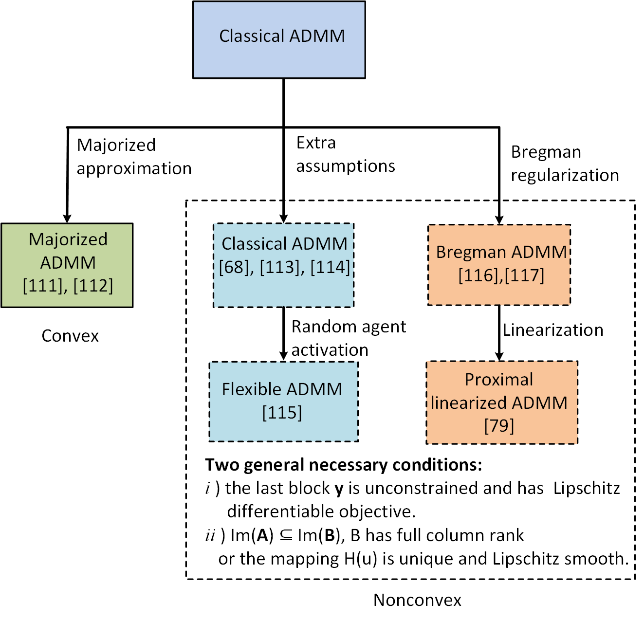
Figure 6: An overview of the relationships of ADMM variants for solving multi-block coupled problem ($\mathbf{P}3$) (solid and dashed boxes indicate convex and nonconvex methods respectively).

IV-C1 Majorized ADMM

For convex multi-block coupled problem ($\mathbf{P}3$) (i.e., $f$, $g$ and $h$ are convex), majorized ADMM has been the main solution [111, 112]. The key idea is to optimize a majorized surrogate of AL problem in a distributed manner. A majorized surrogate represents some approximation of a function from above. For problem ($\mathbf{P}3$), majorized ADMM takes the following general iterative framework.

Majorized ADMM:

$$\textbf{Primal update:}~{}~{}\mathbf{x}_{i}^{k+1}=\arg\min_{\mathbf{x}_{i}}\hat{\mathcal{L}}_{\rho}(\mathbf{x}_{i},\mathbf{x}_{-i}^{k},\mathbf{y}^{k},\bm{\lambda}^{k}),i\in N.$$

$$\quad\quad\quad\quad\quad\quad\quad\mathbf{y}^{k+1}=\arg\min_{\mathbf{y}}\hat{\mathcal{L}}_{\rho}(\mathbf{x}^{k},\mathbf{y},\bm{\lambda}^{k})$$

$$\textbf{Dual update:}~{}\quad\bm{\lambda}^{k+1}=\bm{\lambda}^{k}+\rho(\mathbf{A}\mathbf{x}^{k+1}+\mathbf{B}\mathbf{y}^{k+1})$$

where $\hat{\phi}(\mathbf{x},\mathbf{y})$ represents a majorized surrogate or majorized approximation of objective function $\phi(\mathbf{x},\mathbf{y})$. A majorized surrogate means $\hat{\phi}(\mathbf{x},\mathbf{y})\geq\phi(\mathbf{x},\mathbf{y}),\forall\mathbf{x},\mathbf{y}$. Correspondingly, $\hat{\mathcal{L}}_{\rho}(\mathbf{x},\mathbf{y},\bm{\lambda})=\hat{\phi}(\mathbf{x},\mathbf{y})+\langle\bm{\lambda},\mathbf{A}\mathbf{x}+\mathbf{B}\mathbf{y}\rangle+\frac{\rho}{2}\|\mathbf{A}\mathbf{x}+\mathbf{B}\mathbf{y}\|^{2}$ can be viewed as a majorized surrogate of the AL function.

Majorized ADMM is a conceptual algorithmic framework and its practical implementation requires to determine a proper majorized surrogate $\hat{\phi}(\mathbf{x},\mathbf{y})$. In terms of such issue, some general instructions have been identified [111]. Specifically, let $\mathbf{z}:=(\mathbf{x}^{\top},\mathbf{y}^{\top})^{\top}$ be the stacked primal variables, we have $g(\mathbf{z}):=g(\mathbf{x},\mathbf{y})$ and $\phi(\mathbf{z}):=\phi(\mathbf{x},\mathbf{y})$. A majorized surrogate $\hat{\phi}(\mathbf{x},\mathbf{y})$ for majorized ADMM requires that

• $\hat{\phi}(\mathbf{z})\geq\phi(\mathbf{z}),\forall\mathbf{z}\in{\rm dom}~{}\phi$.

• there exists $\mathbf{u}\in{\rm dom}~{}\phi$ and positive semidefinite matrix $\mathbf{L}$ such that $|\hat{\phi}(\mathbf{z})-\phi(\mathbf{z})|\leq\frac{1}{2}\|\mathbf{z}-\mathbf{u}\|^{2}_{\mathbf{L}},\forall\mathbf{z}\in{\rm dom}~{}\phi$.

• $\hat{\phi}(\mathbf{z})$ is $\mathbf{P}$-strongly convex ($\mathbf{P}$ is positive semidefinite), which states that for any given $\mathbf{z}\in{\rm dom}~{}\phi$, we have $\phi(\mathbf{z})-\frac{1}{2}\|\mathbf{z}-\mathbf{v}\|^{2}_{\mathbf{P}}$ convex.

Some typical majorized surrogates $\hat{\phi(\mathbf{z})}$ for majorized ADMM include [111]

• Proximal surrogate: $\hat{\phi}(\mathbf{z})=\phi(\mathbf{z})+\frac{1}{2}\|\mathbf{z}-\mathbf{z}^{k}\|_{\mathbf{L}}$ for any positive semidefinite matrix $\mathbf{L}$.

• $\operatorname{\text{Lipschitz}}$ surrogate: $\hat{\phi}(\mathbf{z})=\phi(\mathbf{z}^{k})+\langle\nabla\phi(\mathbf{z}^{k}),\mathbf{z}-\mathbf{z}^{k}\rangle+\frac{1}{2}L_{\phi}\|\mathbf{z}-\mathbf{z}^{k}\|^{2}$, where $\phi(\mathbf{z})$ is $L_{\phi}$-$\operatorname{\text{Lipschitz}}$ differentiable.

• Proximal gradient surrogate: $\hat{\phi}(\mathbf{z})=\sum_{i=1}^{n}f_{i}(\mathbf{x}_{i})+h(\mathbf{y})+\langle\nabla g(\mathbf{z}^{k}),\mathbf{z}-\mathbf{z}^{k}\rangle+\frac{1}{2}L_{g}\|\mathbf{z}-\mathbf{z}^{k}\|^{2}$, where $g(\mathbf{z})$ is $L_{g}$-$\operatorname{\text{Lipschitz}}$ differentiable.

where $\mathbf{z}^{k}:=\big{(}(\mathbf{x}^{k})^{\top},(\mathbf{y}^{k})^{\top}\big{)}^{\top}$ is the generated primal updates at iteration $k$. These majorized surrogates can be viewed as some local approximations of the coupled objective $\phi(\mathbf{z})$ from above at each iteration.

Note that majorized ADMM relies on a $\operatorname{Jacobian}$ decomposition to approximate the joint primal update ($\mathbf{y}$ and $\mathbf{x}_{i}$ play the same role in this method). We usually prefer a majorized surrogate $\hat{\phi}(\mathbf{z})$ that is separable across the decision blocks $\mathbf{x}_{i},i\in N$ and $\mathbf{y}$, which favors distributed computation. Besides, it was found that a tight majorized approximation indicated by smaller $|\hat{\phi}(\mathbf{z})-\phi(\mathbf{z})|$ favors convergence speed of the method [111]. For general convex multi-block coupled problem ($\mathbf{P}3$), the convergence and $\mathcal{O}(1/k)$ ergodic convergence rate of the method were established for $\operatorname{\text{Lipschitz}}$ differentiable objective $g$ [111]. For the special two-block convex case (i.e., $\mathbf{x}$ degenerates into one block), [112] established the similar theoretical convergence for the method.

IV-C2 Classic ADMM

As a celebrated work, [68] studied the direct extension of classical ADMM to multi-block coupled problem ($\mathbf{P}3$) in general nonconvex setting. The application of classical ADMM to problem ($\mathbf{P}3$) is standard and takes the following iterative scheme.

Classic ADMM:

$$\textbf{Primal update:}~{}\mathbf{x}_{i}^{k+1}=\arg\min_{\mathbf{x}_{i}}\mathcal{L}_{\rho}(\mathbf{x}_{<i}^{k+1},\mathbf{x}_{i},\mathbf{x}_{>i}^{k},\mathbf{y}^{k},\bm{\lambda}^{k}),\forall i\in N.$$

$$\quad\quad\quad\quad\quad\quad\quad\mathbf{y}^{k+1}=\arg\min_{\mathbf{y}}\mathcal{L}_{\rho}(\mathbf{x}^{k+1},\mathbf{y},\bm{\lambda}^{k})$$

$$\textbf{Dual update:}~{}\quad\bm{\lambda}^{k+1}=\bm{\lambda}^{k}+\rho(\mathbf{A}\mathbf{x}^{k+1}+\mathbf{B}\mathbf{y}^{k+1})$$

Classical ADMM relies on a $\operatorname{Gauss-Seidel}$ decomposition to split the joint primal update. For the coupled objective component $g$, a $\operatorname{Gauss-Seidel}$ decomposition is equivalent to a block coordinate method. The global convergence of classical ADMM towards stationary points was established under the conditions [68]:

• $f_{i}$ are restricted prox-regular.

• $g$ and $h$ are $\operatorname{\text{Lipschitz}}$ differentiable.

• $\mathbf{A}_{i}$ have full column rank or the mappings $F_{i}(\mathbf{u})=\{\arg\min_{\mathbf{x}_{i}}\phi_{i}(\mathbf{x}_{<i},\mathbf{x}_{i},\mathbf{x}_{>i},\mathbf{y}):\mathbf{A}_{i}\mathbf{x}_{i}=\mathbf{u}\}$ are unique and $\operatorname{\text{Lipschitz}}$ smooth.

• ${\rm\mathbf{A}}\subseteq{\rm\mathbf{B}}$, $\mathbf{B}$ has full column rank or the mapping $H(\mathbf{u})=\{\arg\min_{\mathbf{y}}\phi(\mathbf{x},\mathbf{y}):\mathbf{B}\mathbf{y}=\mathbf{u}\}$ is unique and $\operatorname{\text{Lipschitz}}$ smooth.

Restricted prox-regular functions were argued to be broad including but not limited to $\operatorname{\text{Lipschitz}}$ differentiable functions, weakly convex functions and $\ell_{q}$ quasi-norms ($0<q<1$) [68]. The assumptions related to $F_{i}(\mathbf{u})$ and $H(\mathbf{u})$ were claimed as some weaker assumptions of full column rank $\mathbf{A}_{i}$ and $\mathbf{B}$. To our best knowledge, a)-d) have been the most general conditions regarding the convergence of classical ADMM in nonconvex setting.

Note that no convexity is assumed for the problem. This implies that classical ADMM is actually applicable to broad problems provided with conditions a)-d) regardless of convexity. This seems a contraction to our previous results where we concluded that the direct extension of classical ADMM to multi-block optimization is not necessary convergent without any extra strong convexity assumptions (see Section IV-B). Actually, this is caused by the different structures of problem ($\mathbf{P}3$) from ($\mathbf{P}2$). Specifically, ($\mathbf{P}3$) has a special last block $\mathbf{y}$ that satisfies the two conditions: i) the last block $\mathbf{y}$ is unconstrained and has $\operatorname{\text{Lipschitz}}$ differentiable objective (i.e., $g$ and $h$ are $\operatorname{\text{Lipschitz}}$ differentiable w.r.t. $\mathbf{y}$), and ii) the coefficient matrices $\mathbf{A},\mathbf{B}$ satisfy ${\rm Im}(\mathbf{A})\subseteq{\rm Im}(\mathbf{B})$ and $\mathbf{B}$ has full column rank (or the mapping $H(\mathbf{u})$ is unique and $\operatorname{\text{Lipschitz}}$ smooth). We refer to such a last block as a well-behaved last block. This is in the sense that such a last block makes it possible to bound the dual updates $\|\bm{\lambda}^{k+1}-\bm{\lambda}^{k}\|^{2}$ by the primal updates $\|\mathbf{x}^{k+1}-\mathbf{x}^{k+1}\|^{2}$ and $\|\mathbf{y}^{k+1}-\mathbf{y}^{k}\|^{2}$ in the iterative process. This is critical to provide the sufficiently decreasing property of the AL function (viewed as a Lyapunov function) over the iterations, implying the convergent property of generated primal and dual sequences.

While [68] studied a general multi-block coupled problem ($\mathbf{P}3$) in nonconvex setting, some other works considered some special cases. For example, [113] studied the convergence of classical ADMM for a special two-block nonconvex optimization without any coupled objective, i.e., $n=1$, $g=0$, and $\mathbf{B}=\mathbf{I}$. Besides, [114] studied a special $3$-block nonconvex optimization arising from image processing with $n=3$, $g=0$ and $h$ strongly convex and quadratic. These works can be regarded as the special cases of [68] in terms of both problem structures and convergence conditions.

IV-C3 Flexible ADMM

Flexible ADMM can be viewed as a flexible version of classical ADMM [115]. The key idea is to activate the computing agents by a random mechanism. This is often preferred when the computing agents have limited energy or suffer certain random ON/OFF behaviors. The implementation of flexible ADMM is presented below.

Flexible ADMM:

Primal update:

$$\mathbf{x}_{i}^{k+1}\!\!=\!\!\begin{cases}\arg\min_{\mathbf{x}_{i}}\!\mathcal{L}_{\rho}(\mathbf{x}_{<i}^{k+1},\!\mathbf{x}_{i},\!\mathbf{x}_{>i}^{k},\!\mathbf{y}^{k},&\!\!\!\!\!\bm{\lambda}^{k}),\text{ if agent $\mathbf{x}_{i}$ is activated.}\\ \mathbf{x}_{i}^{k},&~{}~{}~{}\text{ if agent $\mathbf{x}_{i}$ not activated.}\end{cases}$$

$$\mathbf{y}^{k+1}\!\!=\!\!\begin{cases}\arg\min_{\mathbf{y}}\mathcal{L}_{\rho}(\mathbf{x}^{k+1},\mathbf{y},\bm{\lambda}^{k}),&\quad\quad\text{ if agent $\mathbf{y}$ is activated.}\\ \mathbf{y}^{k},&\quad\quad\text{ if agent $\mathbf{y}$ not activated.}\end{cases}$$

$$\textbf{Dual update:}~{}\bm{\lambda}^{k+1}=\bm{\lambda}^{k}+\rho(\mathbf{A}\mathbf{x}^{k+1}+\mathbf{B}\mathbf{y}^{k+1})$$

Flexible ADMM employs a random agent activation mechanism in the primal update. As a result, a decision block will be updated only if the related computing agent is activated, otherwise the old update will be held and communicated to the others at each iteration. Clearly, the convergence of flexible ADMM depends on the random agent activation mechanism. For the two usual cases that the agents are all activated with positive probability or in an essentially cyclic manner (i.e., activated at least once within $K$ iterations), the convergence of flexible ADMM towards stationary points has been established for a class of problems with the following structures [115].

• $f_{i}$ are convex or $\operatorname{\text{Lipschitz}}$ differentiable.

• $h$ is $\operatorname{\text{Lipschitz}}$ differentiable and $g=0$.

• $\mathbf{A}_{i}$ have full column rank.

• $\mathbf{B}=\mathbf{I}$.

Note that the above conditions a)-d) are a special case of conditions a)-d) with classical ADMM. To our understanding, the more general conditions a)-d) with classical ADMM are readily extensible to the flexible ADMM since the two methods share the same procedures to establish convergence and the related conditions play the same roles.

IV-C4 Bregman ADMM

For multi-block coupled problem ($\mathbf{P}3$), Bregman ADMM is another ADMM variant for nonconvex optimization [116]. Central to the method is to regularize the subproblems with classical ADMM by some Bregman divergence. Bregman divergence or Bregman distance is one metric for measuring the discrepancy of two points, which includes Eculidean distance as a special case. Compared with classical ADMM, Bregman ADMM does not impose any restrictions on the objective functions $f_{i}$ (i.e., restricted prox-regular) and the coefficient matrices $\mathbf{A}_{i}$, making the method applicable to more general problems. Bregman ADMM takes the following general framework.

Bregman ADMM:

Primal update:

$$~{}\mathbf{x}_{i}^{k+1}=\arg\min\limits_{\mathbf{x}_{i}}\mathcal{L}_{\rho}(\mathbf{x}_{<i}^{k+1},\mathbf{x}_{i},\mathbf{x}_{>i}^{k},\mathbf{y}^{k},\bm{\lambda}^{k})+\Delta_{\phi_{i}}(\mathbf{x}_{i},\mathbf{x}_{i}^{k}),\forall i\in N.$$

$$~{}\mathbf{y}^{k+1}=\arg\min\limits_{\mathbf{y}}\mathcal{L}_{\rho}(\mathbf{x}^{k+1},\mathbf{y},\bm{\lambda}^{k})+\Delta_{\psi}(\mathbf{y},\mathbf{y}^{k})$$

$$\textbf{Dual update:}~{}\bm{\lambda}^{k+1}=\bm{\lambda}^{k}+\rho(\mathbf{A}\mathbf{x}^{k+1}+\mathbf{B}\mathbf{y}^{k+1})$$

where $\Delta_{\phi_{i}}(\cdot,\cdot)$ and $\Delta_{\psi}(\cdot,\cdot)$ are Bregman divergence defined on the convex functions $\phi_{i}$ and $\psi$, respectively. For a general convex differentiable function $\phi:\mathbf{R}^{n}\rightarrow\mathbf{R}$, the related Bregman divergence is defined by

$$\Delta_{\phi}(\mathbf{x},\mathbf{y})=\phi(\mathbf{x})-\phi(\mathbf{y})-\langle\nabla\phi(\mathbf{y}),\mathbf{x}-\mathbf{y}\rangle,~{}\forall\mathbf{x},\mathbf{y}\in\mathbf{R}^{n}.$$

Note that Bregman distance reduces to Eculidean distance $\Delta_{\phi}(\mathbf{x},\mathbf{y})=\|\mathbf{x}-\mathbf{y}\|^{2}$ with $\phi(\mathbf{x})=\|\mathbf{x}\|^{2}$, which has been widely used in proximal ADMM variants as discussed before. For $\phi(\mathbf{x})=\|\mathbf{x}\|^{2}_{\mathbf{Q}}$, we have the resulting Bregman distance $\Delta_{\phi}(\mathbf{x},\mathbf{y})=\|\mathbf{x}-\mathbf{y}\|^{2}_{\mathbf{Q}}$ which has been used in many generalized ADMM variants. From this perspective, we see that the Bregman ADMM defines a general algorithmic framework for solving problem ($\mathbf{P}3$). The practical implementation requires to determine the specific Bregman divergence $\Delta_{\phi_{i}}(\cdot,\cdot)$ and $\Delta_{\psi}(\cdot,\cdot)$. The convergence of Bregman ADMM towards first-order stationary points has been established for a class of problems with the following structures [116].

• $g=0$.

• $h$, $\phi_{i}$, $\varphi$ are $\operatorname{\text{Lipschitz}}$ differentiable.

• $f_{i}$ or $\phi_{i}$, $h$ or $\varphi$ are strongly convex.

• $\mathbf{B}$ has full row rank .

Consider a usual case that Eculidean distance is used as Bregman divergence (i.e., $\phi_{i}(\mathbf{x})=\|\mathbf{x}\|^{2}$ and $\varphi(\mathbf{x})=\|\mathbf{x}\|^{2}$), we clearly have $\phi_{i}$ and $\varphi$ strongly convex and $\operatorname{\text{Lipschitz}}$ differentiable. In such context, conditions a)-d) reduce to $g=0$, $h$ $\operatorname{\text{Lipschitz}}$ differentiable and $\mathbf{B}$ has full row rank. Actually, this represents a special case of conditions b)-d) with classical ADMM. To our understanding, the general conditions b)-d) with classical ADMM can be directly extended to Bregman ADMM if some strongly convex and $\operatorname{\text{Lipschitz}}$ differentiable Bregman divergence functions $\phi_{i}$ and $\varphi$ are selected. This is because the two methods follow the same procedures to establish convergence and the related conditions play similar roles. One benefit resulting from Bregman divergence is that the restricted prox-regular conditions on $f_{i}$ with classical ADMM and the rank assumptions on the coefficient matrices $\mathbf{A}_{i}$ can be relaxed, making the methods applicable to more general problems.

The above results are for the general Bregman ADMM. Some works have studied some special instances of Bregman ADMM. For example, [117] proposed two proximal ADMM variants where the proximal terms $\frac{\tau}{2}\|\mathbf{x}_{i}-\mathbf{x}_{i}^{k}\|^{2}_{\mathbf{P}_{i}}$ and $\frac{L_{\mathbf{y}}}{2}\|\mathbf{y}-\mathbf{y}^{k}\|^{2}$ are used as Bregman divergence. The convergence of the methods was proved under the conditions: i) $g$ and $h$ are $\operatorname{\text{Lipschitz}}$ differentiable, and ii) $\mathbf{B}$ has full row rank, which are in line with a) - d).

IV-C5 Proximal linearized ADMM

Note that the above ADMM variants for problem ($\mathbf{P}3$) require to solve the subproblems exactly at each iteration. This could be expensive or not efficient when the objective functions are complex and coupled. To reduce per-iteration complexity, [79] proposed a proximal linearized ADMM as an inexact ADMM variant. The key idea is to linearize some complex (i.e., often hard to compute proximal mappings) but differentiable parts of the objective components and then solving the resulting easier proximal linearized subproblems. Proximal linearized ADMM takes the following iterative scheme.

Proximal linearized ADMM:

Primal update:

$$\mathbf{x}_{i}^{k+1}\!=\!\arg\min_{\mathbf{x}_{i}}f_{i}(\mathbf{x}_{i})\!+\!l_{i}(\mathbf{x}^{k},\mathbf{y}^{k},\bm{\lambda}^{k})^{\top}(\mathbf{x}_{i}\!-\!\mathbf{x}_{i}^{k})\!+\!\frac{\tau_{\mathbf{x}}}{2}\|\mathbf{x}_{i}\!-\!\mathbf{x}_{i}^{k}\|^{2},i\in N.$$

$$\mathbf{y}^{k+1}\!=\!\arg\min_{\mathbf{y}}u(\mathbf{x}^{k+1},\mathbf{y}^{k},\bm{\lambda}^{k})^{\top}(\mathbf{y}-\mathbf{y}^{k})+\frac{\tau_{\mathbf{y}}}{2}\|\mathbf{y}-\mathbf{y}^{k}\|^{2}$$

$$\textbf{Dual update:}~{}\bm{\lambda}^{k+1}=\bm{\lambda}^{k}+\rho(\mathbf{A}\mathbf{x}^{k+1}+\mathbf{B}\mathbf{y}^{k+1})$$

where $l_{i}(\mathbf{x}^{k},\mathbf{y}^{k},\bm{\lambda}^{k})$ and $u(\mathbf{x}^{k+1},\mathbf{y}^{k},\bm{\lambda}^{k})$ denote the gradients of the differentiable parts of AL function w.r.t. $\mathbf{x}_{i}$ and $\mathbf{y}$ respectively. Specifically, $l_{i}(\mathbf{x}^{k},\mathbf{y}^{k},\bm{\lambda}^{k})$ is obtained by differentiating $g(\mathbf{x},\mathbf{y})+(\bm{\lambda}^{k})^{\top}\mathbf{A}\mathbf{x}+\frac{\rho}{2}\|\mathbf{A}\mathbf{x}+\mathbf{B}\mathbf{y}\|^{2}$ w.r.t. $\mathbf{x}_{i}$ at $(\mathbf{x}^{k},\mathbf{y}^{k})$, and $u(\mathbf{x}^{k+1},\mathbf{y}^{k},\bm{\lambda}^{k})$ is obtained by differentiating $h(\mathbf{y})+g(\mathbf{x},\mathbf{y})+(\bm{\lambda}^{k})^{\top}\mathbf{B}\mathbf{y}+\frac{\rho}{2}\|\mathbf{A}\mathbf{x}+\mathbf{B}\mathbf{y}\|^{2}$ w.r.t. $\mathbf{y}$ at $(\mathbf{x}^{k+1},\mathbf{y}^{k})$. Here we consider a general $f_{i}$ that is probably nonsmooth. If $f_{i}$ is smooth and differentiable, it can be linearized and involved in $l_{i}(\mathbf{x}^{k},\mathbf{y}^{k},\bm{\lambda}^{k})$ similarly. Since a first-order linearization only provides an inaccurate approximation to the AL function, some proximal terms $\frac{\tau_{\mathbf{x}}}{2}\|\mathbf{x}_{i}-\mathbf{x}_{i}^{k}\|^{2}$ and $\frac{\tau_{y}}{2}\|\mathbf{y}-\mathbf{y}^{k}\|^{2}$ are required to control the approximation accuracy.

Slightly different from classical ADMM where ($\mathbf{P}3$) is considered as a multi-block optimization and $\operatorname{Gauss-Seidel}$ decomposition is used to enable a multi-block serial update, proximal linearized ADMM was derived by treating ($\mathbf{P}3$) as a two-block optimization and applying $\operatorname{Gauss-Seidel}$ decomposition to the two decision blocks $\mathbf{x}:=(\mathbf{x}_{i})_{i=1}^{n}$ and $\mathbf{y}$. Due to the linearization, we have subproblems $\mathbf{x}$ naturally decomposable across the decision components $\mathbf{x}_{i}$. This brings the benefit of parallel implementation. Note that subproblems $\mathbf{x}_{i}$ in the primal update reduce to the proximal mappings of $f_{i}$, i.e., $\mathbf{x}_{i}^{k+1}=\arg\min_{\mathbf{x}_{i}}f_{i}(\mathbf{x}_{i})+\frac{\tau_{x}}{2}\|\mathbf{x}_{i}-(\mathbf{x}_{i}^{k}-\tau_{\mathbf{x}}^{-1}l_{i}(\mathbf{x}^{k},\mathbf{y}^{k},\bm{\lambda}^{k}))\|^{2}$, and subproblems $\mathbf{y}$ reduce to a gradient-like iterate, i.e., $\mathbf{y}^{k+1}=\mathbf{y}^{k}-\tau_{\mathbf{y}}^{-1}u(\mathbf{x}^{k+1},\mathbf{y}^{k},\bm{\lambda}^{k})$. If $f_{i}$ has easily computable proximal mappings, we would have low per-iteration complexity with the method. The convergence of proximal linearized ADMM towards stationary points was proved under the conditions [79]:

• $g$ and $h$ are $\operatorname{\text{Lipschitz}}$ differentiable.

• ${\rm Im}(\mathbf{A})\subseteq{\rm Im}(\mathbf{B})$, and $\mathbf{B}$ has full column rank.

Similar to other linearized ADMM variants discussed before, the linearization technique with the method also requires the objective functions to be $\operatorname{\text{Lipschitz}}$ differentiable.

One salient feature of proximal linearized ADMM is that no restrictions on the objective functions $f_{i}$ and the coefficient matrices $\mathbf{A}_{i}$ are required as with classical ADMM. This is caused by the proximal regularization $\frac{\tau_{\mathbf{x}}}{2}\|\mathbf{x}-\mathbf{x}^{k}\|^{2}$ that enhances the convexity of subproblems. As discussed with classical ADMM, the full column rank $\mathbf{B}$ can be replaced by the weaker assumption, i.e., the mapping $H(\mathbf{u})=\{\arg\min_{\mathbf{y}}\phi(\mathbf{x},\mathbf{y}):\mathbf{B}\mathbf{y}=\mathbf{u}\}$ is unique and $\operatorname{\text{Lipschitz}}$ smooth. This holds for proximal linearized ADMM since the two methods follow the same procedures to establish convergence and the related assumptions play the same roles. This implies that proximal linearized ADMM depends on weaker conditions than classical ADMM. As a result, the method is applicable to more general applications, such as sparsity regression [118] and integer programming [79]. Due to the low per-iteration complexity and parallel implementation, proximal linearized ADMM was shown to be advantageous than classical ADMM in computation efficiency [79].

TABLE IV: ADMM variants for solving multi-block coupled problem ($\mathbf{P}3$)

Methods	Main assumptions	Types	Convergence	Features	References
Majorized ADMM	$f,g$ and $h$ convex. $g$ $\operatorname{\text{Lipschitz}}$ differentiable.	$\operatorname{Jacobian}$ or Gauss-Seidel	Global convergence. Global optima. Convergence rate $\mathcal{O}(1/k)$.	Convex.	[112, 111]
Classic ADMM	$f_{i}$ restricted prox-regular. $g$ and $h$ $\operatorname{\text{Lipschitz}}$ differentiable. $\mathbf{A}_{i}$ full column rank or $F_{i}(\mathbf{u})$ unique and $\operatorname{\text{Lipschitz}}$ smooth. $\text{Im}(\mathbf{A})\subseteq\text{Im}(\mathbf{B})$. $\mathbf{B}$ full column rank or $H(\mathbf{u})$ unique and $\operatorname{\text{Lipschitz}}$ smooth.	Gauss-Seidel	Global convergence. Stationary points	Weak assumptions. Nonconvex.	[68]
	$g=0,n=1$. h $\operatorname{\text{Lipschitz}}$ differentiable. $\mathbf{A}_{1}$ full column rank. $\mathbf{B}=\mathbf{I}$	Gauss-Seidel	Global convergence. Stationary points	2-block. No restrictions on $f$. Nonconvex.	[113]
	$g=0,n=3$. $h$ quadratic . $f_{1}$ convex. $f_{2}$ nonconvex and nonsmooth. $\mathbf{A}_{1}$ and $\mathbf{A}_{3}$ full row rank.	Gauss-Seidel	Global convergence. Stationary ponts	3-block. Nonconvex.	[114]
Flexible ADMM	g = 0. $\mathbf{B}=\mathbf{I}$. $f_{i}$ convex or $\operatorname{\text{Lipschitz}}$ differentiable. $\mathbf{A}_{i}$ has full column rank.	Gauss-Seidel	Global convergence. Stationary points.	Random agent activation. Nonconvex.	[115]
Bregman ADMM	g = 0. $f_{i}$ or $\phi_{i}$, $h$ or $\psi$ strongly convex. $h$, $\phi_{i}$, $\psi$ $\operatorname{\text{Lipschitz}}$ differentiable. $\mathbf{B}$ has full row rank.	Gauss-Seidel	Global convergence. Stationary points.	No restrictions on $f_{i}$ and $\mathbf{A}_{i}$. Nonconvex.	[116]
	$g$ and $h$ $\operatorname{\text{Lipschitz}}$ differentiable. $\mathbf{B}=\mathbf{I}$	Gauss-Seidel	Global convergence. Stationary points.	No restrictions on $f_{i}$ and $\mathbf{A}_{i}$. Nonconvex.	[117]
Proximal linearized ADMM	$g$ and $h$ $\operatorname{\text{Lipschitz}}$ differentiable. $\text{Im}(\mathbf{A})\subseteq\text{Im}(\mathbf{B})$. $\mathbf{B}$ full column rank.	Gauss-Seidel + Jacobian	Global convergence. Stationary points.	No restrictions on $f_{i}$ and $\mathbf{A}_{i}$. Low per-iteration complexity. Nonconvex.	[79]

Summary: This section surveys ADMM variants for solving multi-block coupled problem ($\mathbf{P}3$). Several ADMM variants have been developed either for convex or nonconvex optimization. We report those ADMM variants in terms of main assumptions, decomposition schemes (i.e., type), convergence properties, main features and references in TABLE IV. From the results, we draw the following overview. For convex optimization, majorized ADMM is the main solution and guarantees the convergence towards global optima. For nonconvex optimization, classical ADMM, flexible ADMM, Bregman ADMM and proximal linearized ADMM are applicable and ensure the convergence towards stationary points. The nonconvex ADMM variants can be distinguished by their different features. Specifically, Bregman ADMM and proximal linearized ADMM do not require any restrictions on the objective functions $f_{i}$ and the coefficient matrices $\mathbf{A}_{i}$ and thus are applicable to broader applications. Proximal linearized ADMM is favorable for its low per-iteration complexity. Flexible ADMM enables random agent activation mechanism which is beneficial when the computing agents have limited energy or suffer certain random ON/OFF behaviors. Particularly, the ADMM variants for nonconvex optimization generally depend on the two necessary conditions to ensure convergence: i) the last block $\mathbf{y}$ is unconstrained and $\operatorname{\text{Lipschitz}}$ differentiable, and ii) ${\rm Im}(\mathbf{A})\subseteq{\rm Im}(\mathbf{B})$, $\mathbf{B}$ has full column rank or the mapping $H(\mathbf{u})=\{\arg\min_{\mathbf{y}}\phi(\mathbf{x},\mathbf{y}):\mathbf{B}\mathbf{y}=\mathbf{u}\}$ is unique and $\operatorname{\text{Lipschitz}}$ smooth.

IV-D Consensus optimization

Previously, we have focused on multi-block optimization where the agents hold disjoint decision variables. In practice, it is also common to see multi-agent systems where the agents share commonly-owned decision variables but hold private objectives. The leads to the well-known consensus optimization that takes the general formulation of

$$\min_{\mathbf{x}}F(\mathbf{x})=\sum_{i=1}^{n}f_{i}(\mathbf{x}) \mathbf{P}4$$ ()

where $f_{i}:\mathbf{R}^{n}\rightarrow\mathbf{R}$ denote the private objectives of the agents; $\mathbf{x}\in\mathbf{R}^{n}$ is the commonly-owned decision variables; $f_{i}$ may be nonsmooth and a usual case is that some local constraints related to the agents are included in the form of indicator functions.

Note that consensus problem ($\mathbf{P}4$) involves only one block of decision variables that is shared by the agents. This does not correspond to the practice of ADMM or its variants which essentially explore the problem decomposition across decision blocks for distributed optimization. To address such an issue, ADMM variants for consensus optimization ($\mathbf{P}4$) are generally developed based on certain equivalent multi-block reformulations. There are four widely-used reformulations indicated by ($\mathbf{P}4$-1) - ($\mathbf{P}4$-4). A number of ADMM variants have been developed for both convex and nonconvex optimization by applying classical ADMM to those reformulations. An overview of the relationships of the ADMM variants for solving consensus problem ($\mathbf{P}4$) is shown in Fig. 7. We distinguish the convex and nonconvex methods by solid and dashed boxes. These methods are often preferred for different features, such as parallel implementation, networked communication schemes, low per-iteration complexity, random agent activation, and asynchronous computing (robust to communication delays or losses).

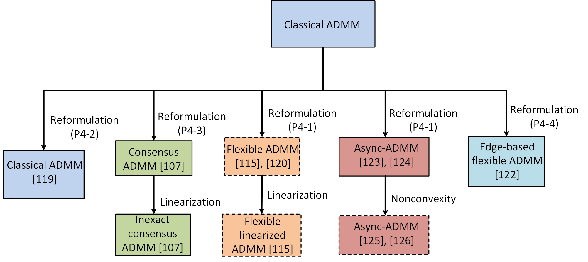
Figure 7: An overview of the relationships of the ADMM variants for solving consensus problem ($\mathbf{P}4$) (the solid and dashed boxes to indicate convex and nonconvex methods respectively).

In the sequel, we introduce each of those methods. Particularly, we first present the four commonly-used reformulations which are helpful to understand the main ideas of related ADMM variants. The reformulations all depend on introducing local decision copies for individual agents and then enforcing the consistency of the decision copies. Their major differences lie in the ways of enforcing consistency constraints. Specifically for problem ($\mathbf{P}4$), one natural and commonly-used reformulation is

$$\min_{\mathbf{x}:=(\mathbf{x}_{i})_{i=0}^{n}}F(\mathbf{x})=\sum_{i=1}^{n}f_{i}(\mathbf{x}_{i}) \mathbf{P}4$$ (-1)

$${\rm s.t.}~{}\mathbf{x}_{i}=\mathbf{x}_{0},~{}\forall i\in N.$$

where $\mathbf{x}_{i}\in\mathbf{R}^{n}$ represents the local decision copy held by agent $i$. To guarantee the consistency of decision copies, a global decision copy $\mathbf{x}_{0}$ is introduced, which is managed by a central coordinator. By enforcing the consistency of all local copies to the global one, i.e., $\mathbf{x}_{i}=\mathbf{x}_{0},\forall i\in N$, we directly have the equivalence of ($\mathbf{P}4$-1) and ($\mathbf{P}4$).

In reformulation ($\mathbf{P}4$-1), the agents are assumed to communicate via a central coordinator. There exist cases that a system is fully decentralized and a central coordinator does not exist. In such context, the agents are restricted to communicate over a network or a graph. We refer to that as networked communication. One direct reformulation that accounts for the networked communication is

$$\min_{\mathbf{x}:=(\mathbf{x}_{i})_{i=1}^{n}}F(\mathbf{x})=\sum_{i=1}^{n}f_{i}(\mathbf{x}_{i}) \mathbf{P}4$$ (-2)

$${\rm s.t.~{}}\mathbf{x}_{i}=\mathbf{x}_{j},\forall(i,j)\in E,i<j.$$

where $\mathbf{x}_{i}\in\mathbf{R}^{n}$ denotes the local decision copy held by agent $i$; $E$ indicates the edges of communication network. To ensure the consistency of decision copies, a hard equality constraint $\mathbf{x}_{i}=\mathbf{x}_{j}$ is imposed for each pair of connected agents, i.e., $(i,j)\in E$. Since we only consider an undirected communication network, one consistency constraint is sufficient for each pair of connected agents and we therefore have $i<j$ in the reformulation.

When the agents are restricted to communicate over a network or a graph, another reformulation is

$$\min_{\mathbf{x}:=(\mathbf{x}_{i})_{i=1}^{n},\mathbf{t}:=(t_{ij})_{i,j=1}^{n}}~{}F(\mathbf{x})=\sum_{i=1}^{n}f_{i}(\mathbf{x}_{i}) \mathbf{P}4$$ (-3)

$${\rm s.t.}~{}~{}\mathbf{x}_{i}=t_{ij},\quad\forall j\in N_{i},i\in N.$$

$$\quad\quad\mathbf{x}_{j}=t_{ij},\quad\forall j\in N_{i},i\in N.$$

where $\mathbf{x}_{i}\in\mathbf{R}^{n}$ denotes the local decision copy held by agent $i$ and $N_{i}$ denotes the set of its neighbors (not including itself). To ensure the consistency of decision copies across the agents, a linking variable $t_{ij}\in\mathbf{R}^{n}$ (also known as slack variable) is introduced for each pair of connected agents (i.e., $j\in N_{i}$ and $i\in N_{j}$). It is easy to show that ($\mathbf{P}4$-3) is equivalent to ($\mathbf{P}4$) for any connected communication network.

Another similar reformulation accounting for networked communication scheme is

$$\min_{\mathbf{x}:=(\mathbf{x}_{i})_{i=1}^{n},\mathbf{z}:=(\mathbf{z}_{ei},\mathbf{z}_{ej})_{e\in E}}F(\mathbf{x})=\sum_{i=1}^{n}f_{i}(\mathbf{x}_{i}) \mathbf{P}4$$ (-4)

$${\rm s.t.~{}}\mathbf{x}_{i}=\mathbf{z}_{ei},~{}\mathbf{x}_{j}=-\mathbf{z}_{ej},\mathbf{z}_{ei}+\mathbf{z}_{ej}=\bm{0},\forall e\in E.$$

where $\mathbf{x}_{i}\in\mathbf{R}^{n}$ denotes the local decision copy held by agent $i$; $E$ denotes the edges of the communication network, i.e., if agent $i,j$ are neighbors, we have $(i,j)\in E$. To ensure the consistency of decision copies held by the agents, two slack variable $\mathbf{z}_{ei}\in\mathbf{R}^{n}$ and $\mathbf{z}_{ej}\in\mathbf{R}^{n}$ are introduced for each edge $e\in E$ that connects agent $i,j$. Clearly, formulation ($\mathbf{P}4$-4) is equivalent to ($\mathbf{P}4$) for any connected communication network.

Note that reformulations ($\mathbf{P}4$-1)-($\mathbf{P}4$-4) all correspond to multi-block linearly constrained optimization where the objective is the sum of private objectives held by the agents. The ADMM variants to be discussed are exactly developed based on the above reformulations. Most of them are the results of the direct application of classical ADMM to the reformulations. However, different problem structures were fruitfully exploited to favor easier implementations.

IV-D1 Classical ADMM

To account for networked communication scheme, [119] studied the direction application of classical ADMM to reformulation ($\mathbf{P}4$-2). Note that problem ($\mathbf{P}4$-2) can be treated as a multi-block optimization with decision variables $\mathbf{x}_{i},i\in N$. The application of classical ADMM to solve multi-block ($\mathbf{P}4$-2) is standard and takes the following iterative scheme.

Classical ADMM:

Primal update:

$$~{}~{}\mathbf{x}_{i}^{k+1}=\arg\min_{\mathbf{x}_{i}}\mathcal{L}_{\rho}\big{(}\mathbf{x}_{i},(\mathbf{x}_{j}^{k+1})_{j<i},(\mathbf{x}_{j}^{k})_{j>i},(\bm{\lambda}_{ji}^{k})_{j<i},(\bm{\lambda}_{ij})^{k}_{i<j}\big{)},$$

$$\quad\quad\quad\quad\quad\quad\quad\quad\quad\forall i\in N.$$

Dual update:

$$~{}~{}\lambda_{ij}^{k+1}=\lambda_{ij}^{k}+\rho(\mathbf{x}_{i}^{k+1}-\mathbf{x}_{j}^{k+1}),\forall(i,j)\in E,i<j.$$

As discussed, the direct extension of classical ADMM to multi-block optimization generally requires some extra conditions (e.g., strongly convex) to ensure convergence. In line with the previous results, [119] established the convergence and $\mathcal{O}(1/k)$ convergence rate of the method for a class of problems with strongly convex objective functions $f_{i}$. Note that the method applies to other consensus problems ($\mathbf{P}4$) that satisfy the necessary conditions of multi-block extension of classical ADMM discussed in Section VI-B.

IV-D2 Consensus ADMM

Consensus ADMM results from the direct application of classical ADMM to reformulation ($\mathbf{P}4$-3) [107]. Note that problem ($\mathbf{P}4$-3) corresponds to a two-block optimization by treating the collections $\mathbf{x}:=(\mathbf{x}_{i})_{i=1}^{n}$ and $\mathbf{t}:=(t_{ij})_{i,j=1}^{n}$ as two decision blocks. When the problem is convex, classical ADMM is directly applicable. For the first block $\mathbf{x}:=(\mathbf{x}_{i})_{i=1}^{n}$, we have the subproblem naturally decomposable across the decision components $\mathbf{x}_{i},i\in N$, and for the second block $\mathbf{t}:=(t_{ij})_{i,j=1}^{n}$, we have quadratic subproblems that admit closed-form solutions. By leveraging the closed-form solutions of the slack variables $\mathbf{t}$, we have the succinct implementation of consensus ADMM below.

Consensus ADMM:

Primal update:

$$\mathbf{x}_{i}^{k+1}=\min_{\mathbf{x}_{i}}f_{i}(\mathbf{x}_{i})+(\bm{\lambda}_{i}^{k})^{\top}\mathbf{x}_{i}+\rho\sum_{j\in N_{i}}\Big{\|}\mathbf{x}_{i}\!-\!\frac{\mathbf{x}_{i}^{k}-\mathbf{x}_{j}^{k}}{2}\Big{\|}^{2},\forall i\in N.$$

$$\textbf{Dual update:}~{}\bm{\lambda}_{i}^{k+1}=\bm{\lambda}_{i}^{k}+\rho\sum_{j\in N_{i}}(\mathbf{x}_{i}^{k+1}-\mathbf{x}_{j}^{k+1}),\forall i\in N.$$

One salient feature of consensus ADMM is the parallelizable implementation. Specifically, the agents are allowed to perform primal updates in a parallel manner. In addition, the method can accommodate a networked communication scheme. Since Consensus ADMM is a direct application of classical ADMM to a two-block convex optimization, its convergence and convergence rate directly follow classical ADMM.

IV-D3 Inexact consensus ADMM

Consensus ADMM requires to solve the subproblems exactly at each iteration. The could be expensive or not efficient when the objective functions $f_{i}$ are complex. To reduce per-iteration complexity, inexact consensus ADMM was proposed as an inexact version of consensus ADMM [107]. The key idea to linearize the subproblems with consensus ADMM and perform an inexact update at each iteration. The method takes the following iterative scheme.

Inexact consensus ADMM:

Primal update:

$$\quad\mathbf{x}_{i}^{k+1}=\min_{\mathbf{x}_{i}}\langle\nabla f_{i}(\mathbf{x}_{i}^{k}),\mathbf{x}_{i}-\mathbf{x}_{i}^{k}\rangle+(\bm{\lambda}^{k}_{i})^{\top}\mathbf{x}_{i}$$

$$\quad\quad\quad\quad+\rho\sum_{j\in N_{i}}\Big{\|}\mathbf{x}_{i}-\frac{\mathbf{x}_{i}^{k}-\mathbf{x}_{j}^{k}}{2}\Big{\|}^{2}+\frac{\tau_{i}}{2}\|\mathbf{x}_{i}-\mathbf{x}_{i}^{k}\|^{2},\forall i\in N.$$

$$\textbf{Dual update:}~{}\bm{\lambda}_{i}^{k+1}=\bm{\lambda}_{i}^{k}+\rho\sum_{j\in N_{i}}(\mathbf{x}_{i}^{k+1}-\mathbf{x}_{j}^{k+1}),\forall i\in N.$$

Note that objective function $f_{i}$ in the primal update is replaced by $\langle\nabla f_{i}(\mathbf{x}_{i}^{k}),\mathbf{x}_{i}-\mathbf{x}_{i}^{k}\rangle+\frac{\tau_{i}}{2}\|\mathbf{x}_{i}-\mathbf{x}_{i}^{k}\|^{2}$ which is a local first-order approximation of $f_{i}$ plus a proximal term (the constant $f_{i}(\mathbf{x}_{i}^{k})$ is discarded). It is easy to note that the resulting subproblems of the primal update admit closed-form solutions and yield low per-iteration complexity. The convergence of inexact consensus ADMM was proved for a class of problems: $f_{i}(\mathbf{x}_{i})=\phi_{i}(\mathbf{A}_{i}\mathbf{x}_{i})$ where $\phi_{i}(\mathbf{x})$ are strongly convex and $\operatorname{\text{Lipschitz}}$ differentiable ($\mathbf{A}_{i}$ can be rank deficient) [107]. Particularly, some convex (possibly nonsmooth) objective functions $g_{i}(\mathbf{x}_{i})$ are admissible and the subproblems should be adapted to $\mathbf{x}_{i}^{k+1}=\min_{\mathbf{x}_{i}}g_{i}(\mathbf{x}_{i})+\langle\nabla f_{i}(\mathbf{x}_{i}^{k}),\mathbf{x}_{i}-\mathbf{x}_{i}^{k}\rangle+(\bm{\lambda}^{k}_{i})^{\top}\mathbf{x}_{i}+\rho\sum_{j\in N_{i}}\big{\|}\mathbf{x}_{i}-\frac{\mathbf{x}_{i}^{k}-\mathbf{x}_{j}^{k}}{2}\big{\|}^{2}+\frac{\tau_{i}}{2}\|\mathbf{x}_{i}-\mathbf{x}_{i}^{k}\|^{2}$, which are proximal linearized subproblems.

IV-D4 Flexible ADMM

Flexible ADMM results from the direction application of classical ADMM to reformulation ($\mathbf{P}4$-1) together with the deployment of a random agent activation mechanism [115, 120]. Note that ($\mathbf{P}4$-1) is a two-block optimization if $\mathbf{x}_{0}$ and $\mathbf{x}:=(\mathbf{x}_{i})_{i=1}^{n}$ are treated as two decision blocks. This corresponds to the problem structures of classical ADMM. The random agent activation mechanism means that the computing agents are activated in a random manner in the iterative process. This is often preferred when the computing agents have limited energy or suffer certain random ON/OFF behaviors. Flexible ADMM takes the following iterative scheme.

Flexible ADMM:

Primal update:

$$\mathbf{x}_{0}^{k+1}\!\!=\!\begin{cases}\arg\min\limits_{\mathbf{x}_{0}}\mathcal{L}_{\rho}(\mathbf{x}_{0},(\mathbf{x}_{i}^{k})_{i=1}^{n},(\bm{\lambda}_{i}^{k})_{i=1}^{n}),\!\!\!\!&\text{if agent $0$ activated}\\ \mathbf{x}_{0}^{k},\!\!\!\!&\text{if agent $0$ not activated.}\\ \end{cases}$$

$$\mathbf{x}_{i}^{k+1}\!=\!\begin{cases}\arg\min\limits_{\mathbf{x}_{i}}\mathcal{L}_{\rho}(\mathbf{x}_{0}^{k+1},\mathbf{x}_{i},\bm{\lambda}_{i}^{k}),&\quad\quad~{}~{}\text{if agent $i$ activated}\\ \mathbf{x}_{i}^{k},&\quad\quad~{}~{}\text{if agent $i$ not activated}\end{cases}$$

$$\textbf{Dual update:}~{}\bm{\lambda}_{i}^{k+1}=\bm{\lambda}_{i}^{k}+\rho(\mathbf{x}_{i}^{k+1}-\mathbf{x}_{0}^{k+1}),i\in N.$$

Note that the primal update of the second block $\mathbf{x}:=(\mathbf{x}_{i})_{i=1}^{n}$ is performed in a distributed and parallel manner due to the naturally decomposable problem structure. Similar to other flexible ADMM variants, the convergence of the method depends on the random agent activation mechanism. For the two usual cases that each agent is activated either with a positive probability at each iteration or in an essentially cyclic manner (i.e., each agent is activated at least once within $K$ iterations), [115, 120] established the convergence of the method for nonconvex optimization with $\operatorname{\text{Lipschitz}}$ differentiable objective functions $f_{i}$. To be noted, the method directly applies to the convex counterpart since it is a direct application of classical ADMM [121]. Particularly, to improve communication efficiency, [121] proposed a group-based communication mechanism for the method where the computing nodes are grouped and the information of nodes are aggregated within groups before communication. Moreover, for convex optimization, the two decision blocks $\mathbf{x}_{0}$ and $\mathbf{x}:=(\mathbf{x}_{i})_{i=1}^{n}$ are interchangeable as the first and second block. This is different from the nonconvex optimization where only $\mathbf{x}:=(\mathbf{x}_{i})_{i=1}^{n}$ can work as the last block. This is because we required a well-behaved last block that satisfies certain $\operatorname{\text{Lipschitz}}$ differentiable and rank properties to ensure convergence in nonconvex setting (see the discussions in Section IV-C).

IV-D5 Flexible linearized ADMM

As an advanced version, flexible linearized ADMM was proposed with the purpose of reducing per-iteration complexity with flexible ADMM [115]. The basic idea is to linearize smooth subproblems and perform an inexact update instead of solving the subproblems exactly at each iteration. Flexible linearized ADMM takes the following iterative scheme.

Linearized flexible ADMM:

Primal update:

$$\mathbf{x}_{0}^{k+1}\!=\!\begin{cases}\arg\min\limits_{\mathbf{x}_{0}}\mathcal{L}_{\rho}(\mathbf{x}_{0},(\mathbf{x}_{i}^{k})_{k=1}^{n},\bm{\lambda}^{k}),~{}~{}\text{if agent $0$ activated.}&\\ \mathbf{x}_{0}^{k},\quad\quad\quad\quad\quad\quad\quad\quad\quad\quad~{}~{}~{}\text{if agent $0$ not activated.}&\end{cases}$$

$$\mathbf{x}_{i}^{k+1}=\begin{cases}\arg\min\limits_{\mathbf{x}_{i}}\langle\nabla f_{i}(\mathbf{x}_{0}^{k+1}),\mathbf{x}_{i}^{k},\bm{\lambda}_{i}^{k}),\mathbf{x}_{i}-\mathbf{x}_{i}^{k}\rangle+\langle\bm{\lambda}_{i}^{k},\mathbf{x}_{i}\rangle&\\ \quad+\frac{\tau_{i}}{2}\|\mathbf{x}_{i}-\mathbf{x}_{i}^{k}\|^{2},\quad\quad\quad~{}~{}~{}~{}~{}\text{if agent $i$ activated.}&\\ \mathbf{x}_{i}^{k},\quad\quad\quad\quad\quad\quad\quad\quad\quad\quad~{}\text{if agent $i$ not activated.}&\end{cases}$$

$$\textbf{Dual update:}~{}\bm{\lambda}_{i}^{k+1}=\bm{\lambda}_{i}^{k}+\rho(\mathbf{x}_{i}^{k+1}-\mathbf{x}_{0}^{k+1}),\forall i\in N.$$

Note that the objective functions $f_{i}$ are linearized at $\mathbf{x}_{i}=\mathbf{x}_{0}^{k+1}$ and some proximal terms $\frac{\tau_{i}}{2}\|\mathbf{x}_{i}-\mathbf{x}_{i}^{k}\|^{2}$ are added to the subproblems to control the linear approximation accuracy. The convergence of flexible linearized ADMM was established under the same conditions as with flexible ADMM, i.e., the objective functions $f_{i}$ are $\operatorname{\text{Lipschitz}}$ differentiable [115]. Note that we can also choose to linearize $f_{i}$ at $\mathbf{x}_{i}=\mathbf{x}_{i}^{k}$ and the theoretical proof can be adapted accordingly.

IV-D6 Edge-based flexible ADMM

Edge-based flexible ADMM is another ADMM variant that adopts a random agent activation mechanism [122]. The major difference from flexible ADMM and its linearized version is that the agents are randomly activated by the edges of their communication network. Specifically at each iteration, a subset of the edges of the communication network are randomly selected and the agents connected to those edges will be activated to perform new updates. This is often referred to random edge-based agent activation mechanism. Edge-based flexible ADMM can be regarded as the result of applying classical ADMM to the reformulation ($\mathbf{P}4$-4) together with the deployment of the random edge-based agent activation mechanism. Note that problem ($\mathbf{P}4$-4) corresponds to a two-block optimization by viewing the collections $\mathbf{x}:=(\mathbf{x}_{i})_{i=1}^{n}$ and $\mathbf{z}:=(\mathbf{z}_{ei},\mathbf{z}_{ej})_{(i,j)\in e,e\in E}$ as two decision blocks. Edge-based flexible ADMM takes the general iterative framework

Edge-based flexible ADMM:

if edge $$e\in E (i,j)\in e$$ is selected, the corresponding agents

will perform the following primal and dual updates.

Primal update:

$$\begin{cases}\mathbf{x}_{i}^{k+1}=\arg\min_{\mathbf{x}_{i}}\mathcal{L}_{\rho}(\mathbf{x}_{i},\mathbf{z}_{ei}^{k},u_{e}^{k})\\ \mathbf{x}_{j}^{k+1}=\arg\min_{\mathbf{x}_{j}}\mathcal{L}_{\rho}(\mathbf{x}_{j},\mathbf{z}_{ej}^{k},v_{e}^{k})\\ \end{cases}$$

$$(\mathbf{z}_{ei}^{k+1},\mathbf{z}_{ej}^{k+1})=\begin{cases}\arg\min_{\mathbf{z}_{ei},\mathbf{z}_{ej}}\mathcal{L}_{\rho}(\mathbf{x}_{i}^{k+1},\mathbf{x}_{j}^{k+1},\mathbf{z}_{ei},\mathbf{z}_{ej},u_{e}^{k},v_{e}^{k})\\ {\rm s.t.~{}}\mathbf{z}_{ei}+\mathbf{z}_{ej}=0.\\ \end{cases}$$

$$\textbf{Dual update:}~{}u_{e}^{k+1}=u_{e}^{k}+\rho(\mathbf{x}_{i}^{k+1}-\mathbf{z}_{ei}^{k+1})$$

$$\quad\quad\quad\quad\quad\quad v_{e}^{k+1}=v_{e}^{k}+\rho(\mathbf{x}_{j}^{k+1}+\mathbf{z}_{ej}^{k+1})$$

where $u_{e}\in\mathbf{R}^{n}$ and $v_{e}\in\mathbf{R}^{n}$ are Lagrangian multipliers associated with the consistency constraints $\mathbf{x}_{i}=\mathbf{z}_{ei},~{}\mathbf{x}_{j}=-\mathbf{z}_{ej}$ in the reformulation ($\mathbf{P}4$-4).

One may note that the subproblems related to decision variables $\mathbf{z}_{ei}$ and $\mathbf{z}_{ej}$ are quadratic and admit close-form solutions: $\mathbf{z}_{ej}^{k+1}=-\frac{u_{e}^{k}+v_{e}^{k}}{2\rho}-\frac{1}{2}(\mathbf{x}_{i}^{k+1}+\mathbf{x}_{j}^{k+1})$ and $\mathbf{z}_{ei}^{k+1}=\frac{u_{e}^{k}+v_{e}^{k}}{2\rho}+\frac{1}{2}(\mathbf{x}_{i}^{k+1}+\mathbf{x}_{j}^{k+1})$, which can be easily derived based on KKT conditions. Similar to other flexible ADMM variants, edge-based flexible ADMM enables flexible implementation and is often preferred when the agents have limited energy. The convergence of the method also depends on the random edge-based agent activation mechanism. For the usual case where each edge is activated with a positive probability at each iteration, the convergence of the method towards global optima was established for convex optimization [122]. Further, an $\mathcal{O}(1/k)$ convergence rate that characterizes the difference of objective gap and the feasibility violation under expectation was established.

IV-D7 Async-ADMM

Note that the above ADMM variants are all implemented in a synchronous manner. The synchronization is in two senses: i) each agent waits for the information of its all interconnected agents to perform a new update , and ii) each agent uses the updated information of its interconnected agents to perform a new update. In practice, there often exist communication delays or losses caused by multiplied factors, such as limited network bandwidth, diverse processor configurations or inhomogeneous agent workloads, etc. In such context, the computing agents of a synchronous ADMM may have to wait a long time for the updated information of their interconnected agents over the network, thus disrupting or degrading the the computation efficiency and scaling property of the method. To address such an issue, a number of works have studied the asynchronous implementation of ADMM variants. In contrast, an asynchronous implementation means that i) each agent only waits for the information of its partial interconnected agents to perform a new update, and ii) each agent is allowed to use some outdated information of its interconnected agents to perform a new update. As some typical examples, [123, 124, 125, 126] studied the asynchronous implementation of flexible ADMM. In flexible ADMM, the agents are distinguished by one master and $n$ workers. The master refers to the central coordinator managing the global decision copy $\mathbf{x}_{0}$ and the workers are agents updating the local decision copies $\mathbf{x}_{i},\forall i\in N$. Note the communications of the method are restricted to the master and the $n$ workers. An synchronous implementation defines that the master waits for the information of all workers to proceed a new update. Clearly, when the number of works is large, the master may have to wait a long time due to the possible communication delays or losses. As a remedy, [123, 124, 125, 126] proposed to allow the master to perform a new update only with the information of partial workers. Moreover, the information is not necessarily updated due to the lack of global synchronized iteration counter. This leads to the asynchronous ADMM (async-ADMM) that takes the following iterative scheme.

Async-ADMM:

Primal update:

$$\text{Master}:\begin{cases}&\mathbf{x}_{i}^{k}=\begin{cases}\hat{\mathbf{x}_{i}},&\text{if}~{}i\in\mathcal{A}_{k}\\ \mathbf{x}_{i}^{k},&\text{if}~{}i\in\mathcal{A}_{k}^{c}\end{cases}\\ &\bm{\lambda}_{i}^{k}=\begin{cases}\hat{\bm{\lambda}}_{i},&\text{if}~{}i\in\mathcal{A}_{k}\\ \bm{\lambda}_{i}^{k},&\text{if}~{}i\in\mathcal{A}_{k}^{c}\\ \end{cases}\\ &d_{i}=\begin{cases}0,&\text{if}~{}i\in\mathcal{A}_{k}\\ d_{i}+1,&\text{if}~{}i\in\mathcal{A}_{k}^{c}\end{cases}\\ &\!\!\!\text{Wait until $|\mathcal{A}_{k}|\geq S$ and $d_{i}\leq\tau-1$:}\\ &\!\!\!\quad\mathbf{x}_{0}^{k+1}=\arg\min\limits_{\mathbf{x}_{0}}\mathcal{L}_{\rho}(\mathbf{x}_{0},(\mathbf{x}_{i}^{k})_{k=1}^{N},\bm{\lambda}^{k}),\\ &\!\!\!\text{Send $\mathbf{x}_{0}^{k+1}$ to the nodes $\mathcal{A}_{k}$.}\\ \end{cases}$$

$$\text{Worker}~{}i:\begin{cases}&\!\!\!\text{Wait until $\hat{\mathbf{x}}_{0}$ arrives}:\\ &\!\!\!\mathbf{x}_{i}^{k_{i}+1}=\arg\min\limits_{\mathbf{x}_{i}\in\mathbf{\mathcal{X}}_{i}}\mathcal{L}_{\rho}(\hat{\mathbf{x}}_{0},\mathbf{x}_{i},\bm{\lambda}_{i}^{k_{i}})\\ \end{cases},~{}\forall i\in N.$$

$$\textbf{Dual update:}~{}\bm{\lambda}^{k_{i}+1}_{i}=\bm{\lambda}_{i}^{k_{1}}+\rho(\mathbf{x}_{i}^{k_{i}+1}-\hat{\mathbf{x}}_{0}),~{}\forall i\in N.$$

where the decision variables with a hat (i.e., $\hat{\mathbf{x}}_{i}$, $\hat{\bm{\lambda}}_{i}$ and $\hat{\mathbf{x}}_{0}$) denote the new information received from related agents by the master. Since the agents behave in an asynchronous manner, each agent holds a private iteration counter. We denote the iteration counter of master and worker by $k$ and $k_{i},i\in N$, respectively. In async-ADMM, the master and workers behave in a slightly different manner due to the communication scheme.

For the master, the workers are distinguished by whether their new updates have arrived or not at each iteration $k$. Specifically, $\mathcal{A}_{k}$ and $\mathcal{A}_{k}^{c}$ indicate the sets of workers whose new updates have arrived or not, respectively. To ensure convergence, the master will set a maximum tolerable delay bound $\tau$ for each individual worker. This states that at least one new update must be served by each individual worker within $\tau$ successive iterations of the master. In other words, the information of the workers used by the master can be at most $\tau$ outdated. To enforce the maximum tolerable delay constraints, a delay counter $d_{i}$ is set for each individual worker. At each iteration, if a new update is received from worker $i$, the delay counter will be cleared (i.e., $d_{i}=0$), otherwise it will be increased by $1$ (i.e., $d_{i}=d_{i}+1$). In async-ADMM, instead of waiting for the new updates of all workers to arrive, the master will proceed a new update with the new information of only partial workers. This is referred to partial synchronization. A specific partial synchronization mechanism $S$ states that the master will proceed a new iterate after receiving the new updates from any $S$ workers and confirming that the remaining workers are not to exceed the maximum tolerable delay bound $\tau$. For the special case that certain remaining workers are to exceed the bound $\tau$ ($d_{i}=\tau-1$), the master will hold on and wait for the new updates of those workers. Note that when we have $S=n$ and $\tau=1$, async-ADMM reduces to synchronous ADMM. In the algorithmic implementation, we use $\mathbf{x}_{i}^{k}$ and $\bm{\lambda}_{i}^{k}$ to denote the latest updates of worker $i$ hold by the master at iteration $k$. To be noted, they may not be the latest update of the workers due to the communication delays or losses. Note that if a new update $\hat{\mathbf{x}}_{i}$ is received from worker $i$, $\mathbf{x}_{i}^{k}$ will be updated accordingly, i.e., $\mathbf{x}_{i}^{k}=\hat{\mathbf{x}}_{i}$ by the master, otherwise the old updates will be hold to perform a new update.

For the worker, the update scheme is slightly different. Since each worker only requires information from the single master, each worker $i$ will wait the new information of the mater to perform a new update.

The convergence of async-ADMM has been studied for both convex [123, 124] and nonconvex [125, 126] optimization. One common and important condition to ensure convergence is that the communication delay is bounded which states that a new update from each individual worker must be served to the master with a limited number of iterations (i.e., $\tau$). For convex optimization, [123] established the worst-case iteration complexity $\mathcal{O}(\frac{n\tau}{kS})$. We imply that the convergence rate of async-ADMM closely relates to the problem scale $n$, the maximum tolerable delay bound configuration $\tau$, and the partial synchronization mechanism $S$. There usually exists a trade-off between the iteration complexity (the number of iterations) and the waiting time of async-ADMM. Specifically, a larger tolerable delay bound $\tau$ and smaller synchronization $S$ often lead to less waiting time but more iterations to converge and vice verse. For the special convex case where $f_{i}$ are strongly convex and $\operatorname{\text{Lipschitz}}$ differentiable, a linear convergence of async-ADMM was established in [125].

IV-D8 Summary

This section reviewed ADMM variants for solving consensus problem ($\mathbf{P}4$). A number of ADMM variants have been developed either for convex or nonconvex settings. We report those ADMM variants in terms of main assumptions, decomposition schemes (i.e., type), convergence properties, main features and references in TABLE V. We see that these ADMM variants can be distinguished by their features. Consensus ADMM and inexact consensus ADMM enables full parallel computation and can accounts for networked communication. Flexible ADMM, flexible linearized ADMM and edge-based flexible ADMM allow a random agent activation mechanism to save the energy consumption of agents. Async-ADMM enables asynchronous computing and is robust to communication delays or losses. Inexact consensus ADMM and flexible linearized ADMM are advantageous with low per-iteration complexity. Particularly, we conclude that the ADMM variants for nonconvex consensus problem ($\mathbf{P}4$) require the objective functions $f_{i}$ to be $\operatorname{\text{Lipschitz}}$ differentiable. This is in line with our discussions on the necessary conditions of nonconvex optimization in Section IV-C.

TABLE V: ADMM variants for solving consensus problem ($\mathbf{P}4$)

Methods	Main assumptions	Types	Convergence	Features	References
Classical ADMM	$f_{i}$ strongly convex.	Gauss-Seidel	Global convergence. Global optima. Convergence rate $\mathcal{O}(1/k)$.	Networked communication. Convex.	[119]
Consensus ADMM	$f_{i}$ convex.	Gauss-Seidel	Global convergence. Global optima.	Parallel implementation. Networked communication. Convex.	[107]
Inexact consensus ADMM	$f_{i}(\mathbf{x})=\phi_{i}(\mathbf{A}_{i}\mathbf{x}_{i})+g_{i}(\mathbf{x}_{i})$ $\phi_{i}$ strongly convex and $\operatorname{\text{Lipschitz}}$ differentiable. $g_{i}$ convex (possibly nonsmooth). $\mathbf{A}_{i}$ can be rank deficient.	Gauss-Seidel	Global convergence. Global optima.	Parallel implementation. Networked communication. Low per-iteration complexity. Convex.	[107]
Flexible ADMM	$f_{i}$ $\operatorname{\text{Lipschitz}}$ differentiable.	Gauss-Seidel	Global convergence. Stationary points.	Random agent activation. Nonconvex	[115, 120]
Flexible linearized ADMM	$f_{i}$ $\operatorname{\text{Lipschitz}}$ differentiable.	Gauss-Seidel	Global convergence. Stationary points.	Random agent activation. Low per-iteration complexity. Nonconvex.	[115]
Edge-based flexible ADMM	$f_{i}$ convex.	Gauss-Seidel	Probability convergence. Global optima. Convergence rate $\mathcal{O}(1/k)$.	Random agent activation. Networked communication. Convex.	[122]
Async-ADMM	$f_{i}$ convex. Bounded delay $\tau$.	Gauss-Seidel	Global convergence. Global optima. Convergence rate $O(\tau/k)$.	Robust to communication delays (asynchronous computing). Networked communication. Convex.	[123, 124]
	$f_{i}$ $\operatorname{\text{Lipschitz}}$ differentiable. Bounded delay $\tau$.	Gauss-Seidel	Global convergence. Stationary points.	Robust to communication delays. (asynchronous computing) Networked communication. Nonconvex.	[125, 126]

IV-E Non-linearly constrained optimization

So far, we have focused on linearly constrained optimization. In other words, the couplings across the agents can be characterized by some linear constraints. In practice, many other systems exist in which the interactions across the agents or subsystems are complex, leading to non-linear coupled constraints. Examples include but not limited to building thermal comfort management [23, 24] and power system control [127, 128]. This class of problems takes the general formulation of

$$\min_{\mathbf{x}=\{x_{i}\}_{i=1}^{n}}\sum_{i=1}^{n}f_{i}(x_{i}) \mathbf{P}5$$ ()

s.t. $$h_{i}(x_{i},\{x_{j}\}_{j\in N_{i}})=0,\quad\forall i\in N.$$

$$g_{i}(x_{i},\{x_{j}\}_{j\in N_{i}})\leq 0,\quad\forall i\in N.$$

$$x_{i}\in X_{i},\quad\quad\quad\quad\quad\quad~{}\forall i\in N.$$

where $f_{i}:\mathbf{R}^{n_{i}}\rightarrow\mathbf{R}$ are private objectives of the agents defined on their decision variables $x_{i}\in\mathbf{R}^{n_{i}},i\in N$; $h_{i}:\mathbf{R}^{\sum_{j\in N_{i}}n_{j}}\rightarrow\mathbf{R}$ and $g_{i}:\mathbf{R}^{\sum_{j\in N_{i}}n_{j}}\rightarrow\mathbf{R}$ characterize the non-linear (often nonconvex) couplings between agent $i$ and its neighbors $N_{i}$. The subset $X_{i}$ represents the local bounded convex constraints of agent $i$. Problem ($\mathbf{P}5$) models a class of multi-agent optimization where the agents hold private objectives but their decisions are coupled in non-linear (often nonconvex) equality and inequality constraints. Currently, distributed methods to handle problem ($\mathbf{P}5$) (often nonconvex) efficiently are extremely lacking.

Though ADMM variants for diverse classes of linearly constrained optimization are available, extending them to non-linearly constrained problem ($\mathbf{P}5$) (often with nonconvex couplings) is nontrivial due to the difficulty to establish convergence. Currently, the existing ADMM variants for solving problem ($\mathbf{P}5$) are quite limited. To our best knowledge, the two-level ADMM proposed in [129] has been the main solution with convergence guarantee. We discuss that method below.

IV-E1 Two-level ADMM

As a celebrated work, [129] studied a two-level ADMM for solving non-linearly constrained problem ($\mathbf{P}5$) in general nonconvex setting (i.e., $f_{i}$, $h_{i}$, $g_{i}$ are nonconvex). The basic idea is to first convert problem ($\mathbf{P}5$) into a linearly constrained optimization and then explore the application of existing ADMM variants. Though the idea is natural, there are some intrinsic challenges to be overcome, i.e., the two necessary conditions (see the discussions in Section IV-C) to ensure the convergence of ADMM and its variants in nonconvex setting can not be provided simultaneously. To overcome such a challenge, two-level ADMM proposed the idea of introducing a block of slack variables as the last block. The idea of this method should be clear from below.

Specifically, by introducing decision copies for the interconnected agents, we have the following equivalent linearly constrained reformulation for problem ($\mathbf{P}5$).

$$\min_{\mathbf{x}=(\mathbf{x}_{i})_{i=1}^{n},\bar{\mathbf{x}}} F(\mathbf{x})=\sum_{i=1}^{n}f_{i}(\mathbf{x}_{i}) \mathbf{P}5$$ (-1)

s.t. $$\sum_{i=1}^{n}\mathbf{A}_{i}\mathbf{x}_{i}+\mathbf{B}\bar{\mathbf{x}}=\bm{0}.$$

$$h_{i}(\mathbf{x}_{i})=\bm{0},g_{i}(\mathbf{x}_{i})\leq\bm{0},$$

$$\mathbf{x}_{i}\in\mathbf{\mathcal{X}}_{i},\quad i\in N.$$

$$\bar{\mathbf{x}}\in\bar{\mathbf{X}}.$$

where $\mathbf{x}_{i}:=(x_{i},(x_{j})_{j\in N_{i}})$ denotes the augmented decision variable held by agent $i$, which consists of its own decision variable $x_{i}$ and the estimates $(x_{j})_{j\in N_{i}}$ for its neighbors indexed by subset $N_{i}$; $\bar{\mathbf{x}}:=(x_{i})_{i=1}^{n}$ represents a global copy of all decision variables over the network. The coupled linear constraints $\sum_{i=1}^{n}\mathbf{A}_{i}\mathbf{x}_{i}+\mathbf{B}\bar{\mathbf{x}}=\bm{0}$ enforce the consistency of the decision copies over the network. By defining $\mathbf{A}:=(\mathbf{A}_{i})_{i=1}^{n}$ and $\mathbf{x}:=(\mathbf{x}_{i})_{i=1}^{n}$, the coupled linear constraints can be expressed by the compact form of $\mathbf{A}\mathbf{x}+\mathbf{B}\bar{\mathbf{x}}=\bm{0}$; $\mathbf{\mathcal{X}}_{i}:=\cup_{j\in N_{i}}X_{j}$ denotes the augmented local constraints for agent $i$.

Note that problem ($\mathbf{P}5$-1) corresponds to a two-block optimization by treating the decision variables $\mathbf{x}:=(\mathbf{x}_{i})_{i=1}^{n}$ and $\bar{\mathbf{x}}$ as two decision blocks. This corresponds to the problem structure of most existing ADMM variants. However, they are not applicable due to the existence of nonconvexity. As discussed in Section VI-C, we generally require a well-behaved last block $\mathbf{y}$ satisfying the two necessary conditions to ensure convergence: i) the last decision block $\mathbf{y}$ is unconstrained and has $\operatorname{\text{Lipschitz}}$ differentiable objective, and ii) ${\rm Im}(\mathbf{A})\subseteq{\rm Im}(\mathbf{B})$, $\mathbf{B}$ has full column rank or the mapping $H(\mathbf{u})=\{\arg\min_{\mathbf{y}}\phi(\mathbf{x},\mathbf{y}):\mathbf{B}\mathbf{y}=\mathbf{u}\}$ is unique and $\operatorname{\text{Lipschitz}}$ smooth. Here $\phi(\mathbf{x},\mathbf{y})$ refers to the objective of problem ($\mathbf{P}5$-1), $\mathbf{B}$ denotes the coefficient matrix of a last block $\mathbf{y}$ and $\mathbf{A}$ represents an augmented coefficient matrix for the decision blocks excluding $\mathbf{y}$. Despite the direct linearly constrained reformulation ($\mathbf{P}5$-1), it was argued that the two necessary conditions i)-ii) can not be provided simultaneously. Specifically, to fulfill condition ii), we should have $\mathbf{x}:=(\mathbf{x}_{i})_{i=1}^{n}$ work as the last block (we actually have ${\rm Im}(\mathbf{A})\supseteq{\rm Im}(\mathbf{B})$ in ($\mathbf{P}5$-1)). However, the presence of local constraints (i.e., $\mathbf{\mathcal{X}}_{i},h_{i},g_{i}$) makes the subproblems $\mathbf{x}$ nonsmooth, violating condition i). Oppositely, if we assume $\bar{\mathbf{x}}$ as the last block, we do not have condition ii). To overcome such a challenge, a block of slack variables $\mathbf{z}$ is introduced as a well-behaved last block. This leads to the following equivalent three-block linearly constrained reformulation.

$$\min_{\mathbf{x}:=(\mathbf{x}_{i})_{i=1}^{n},\bar{\mathbf{x}},\mathbf{z}} F(\mathbf{x})=\sum_{i=1}^{n}f_{i}(\mathbf{x}_{i}) \mathbf{P}5$$ (-2)

s.t. $$\mathbf{A}\mathbf{x}+\mathbf{B}\bar{\mathbf{x}}+\mathbf{z}=\bm{0}.$$

$$h_{i}(\mathbf{x}_{i})=\bm{0},g_{i}(\mathbf{x}_{i})\leq\bm{0},$$

$$\mathbf{x}_{i}\in\mathbf{\mathcal{X}}_{i},\quad i\in N.$$

$$\bar{\mathbf{x}}\in\bar{\mathbf{X}}.$$

$$\mathbf{z}=\bm{0}.$$

On top that, a two-level ADMM variant was proposed for solving ($\mathbf{P}5$-2) in which an ALM is used in the upper level to gradually force the slack variables to zero and the classical ADMM is used in the lower level to solve some relaxed multi-block optimization with the slack variables as the last block. The method takes the following two-loop iterative scheme.

Two-level ADMM:

$$\!\!\!\!\!\text{Outer-loop}\begin{cases}&\!\!\!\!\!\!\text{Inner-loop}\begin{cases}&\!\!\!\textbf{Primal update:}{}\\ &\!\!\!\mathbf{x}^{k+1}\!=\!\arg\min_{\mathbf{x}}\mathcal{L}_{\rho}(\mathbf{x},\bar{\mathbf{x}}^{k},\mathbf{z}^{k},\bm{\lambda}^{k},\bm{\gamma}^{p})\\ &\!\!\!\bar{\mathbf{x}}^{k+1}\!=\!\arg\min_{\bar{\mathbf{x}}}\mathcal{L}_{\rho}(\mathbf{x}^{k+1},\bar{\mathbf{x}},\mathbf{z}^{k},\bm{\lambda}^{k},\bm{\gamma}^{p})\\ &\!\!\!\mathbf{z}^{k+1}\!=\!\arg\min_{\mathbf{z}}\mathcal{L}_{\rho}(\mathbf{x}^{k+1},\bar{\mathbf{x}}^{k+1},\mathbf{z},\bm{\lambda}^{k},\bm{\gamma}^{p})\\ &\!\!\!\!\!\!\textbf{Dual update:}\\ &\bm{\lambda}^{k+1}\!=\!\bm{\lambda}^{k}+\rho(\mathbf{A}\mathbf{x}^{k+1}+\mathbf{B}\bar{\mathbf{x}}^{k+1}+\mathbf{z}^{k+1})\\ \end{cases}\\ &\!\!\!\textbf{Dual update:}~{}~{}\bm{\gamma}^{p+1}=\bm{\gamma}^{p}+\beta\mathbf{z}^{k+1}\end{cases}$$

where $\bm{\lambda}$ and $\bm{\gamma}$ are Lagrangian multipliers associated with the coupled linear constraints $\mathbf{A}\mathbf{x}+\mathbf{B}\bar{\mathbf{x}}+\mathbf{z}=\bm{0}$ and the hard constraints $\mathbf{z}=\bm{0}$; $\rho$ and $\beta$ are penalty parameters for the ADMM in the lower level (Inner-loop) and the ALM in the upper level (Outer-loop); $k$ and $p$ are related iteration counters. In the primal update of Inner-loop, we have the subproblems $\mathbf{x}:=(x_{i})_{i=1}^{n}$ naturally decomposable across the decision components $\mathbf{x}_{i},i\in N$ and thus can be performed in a distributed and parallel manner. The convergence of the two-level ADMM towards stationary points was established for general nonconvex optimization [129]. Further, the efficacy of the method was demonstrated by a concrete application to power system control [128].

Summary: This section reviewed ADMM variants for solving non-linearly constrained problem ($\mathbf{P}5$) (often nonconvex). Currently, this related methods are quite limited. One solution with convergence guarantee is the two-level ADMM. This is mainly caused by the intrinsic challenges that the two necessary conditions to ensure convergence of ADMM variants in nonconvex setting are not satisfied simultaneously. Two-level ADMM proposed the idea of introducing slack variables to fulfill such two conditions. Though the efficacy of the method has been demonstrated both theoretically and empirically, the implementation is generally at the cost of high iteration complexity caused by the two-level iterative scheme.

V Discussions and future research directions

Based on the previous survey, this section discusses several important future research directions related to ADMM and its variants for distributed optimization.

V-A Nonconvex extensions

From this survey, we see that ADMM and its variants for convex optimization have been studied extensively and broad results are now available for broad classes of problems. However, for the more broad nonconvex counterparts, the related solutions are still quite limited. Moreover, the existing ADMM variants for nonconvex optimization are all restricted to the two necessary conditions [68, 129]: i) the last block $\mathbf{y}$ is unconstrained and has $\operatorname{\text{Lipschitz}}$ differentiable objective, and ii) ${\rm Im}(\mathbf{A})\subseteq{\rm Im}(\mathbf{B})$, $\mathbf{B}$ has full column rank or the mapping $H(\mathbf{u})=\{\arg\min_{\mathbf{y}}\phi(\mathbf{x},\mathbf{y}),{\rm s.t.~{}}\mathbf{B}\mathbf{y}=\mathbf{u}\}$ is unique and $\operatorname{\text{Lipschitz}}$ smooth (see the discussions in Section IV-C). There exist a wide spectrum of problems that fail to satisfy such two conditions, such as problems ($\mathbf{P}2$) and ($\mathbf{P}5$). In such situations, it represents a big challenge to develop an ADMM variant with convergence guarantee.

To figure out the solutions, we require to comprehensively understand the general framework of establishing convergence for an ADMM or its variant in nonconvex setting. Specifically, the key step is to identify a sufficiently decreasing and lower bounded Lyapunov function, which can indicate the convergent property of generated sequences. The sufficiently decreasing and lower boundness properties of a Lyapunov function for an ADMM or its variant state that [68, 115]

$$T(\mathbf{x}^{k+1},\bm{\lambda}^{k+1})-T(\mathbf{x}^{k},\bm{\lambda}^{k})$$

$$\quad\quad\quad\quad\leq-\alpha_{\mathbf{x}}\|\mathbf{x}^{k+1}-\mathbf{x}^{k}\|^{2}-\alpha_{\bm{\lambda}}\|\bm{\lambda}^{k+1}-\bm{\lambda}^{k}\|^{2},$$

$$T(\mathbf{x}^{k},\bm{\lambda}^{k})>-\infty,$$

where $T(\cdot,\cdot)$ denotes a general Lyapunov function; $\{\mathbf{x}^{k}\}_{k=1}^{K}$ and $\{\bm{\lambda}^{k}\}_{k=1}^{K}$ are primal and dual sequences; $k$ is the iteration counter; $\alpha_{\mathbf{x}}$ and $\alpha_{\bm{\lambda}}$ are positive scalars. The AL functions and their variants are often used as the Lyapunov functions (see [68] for example). To identify such a Lyapunov function, we generally require to bound the dual updates $\|\bm{\lambda}^{k+1}-\bm{\lambda}^{k}\|^{2}$ by the primal updates $\|\mathbf{x}^{k+1}-\mathbf{x}^{k}\|^{2}$. Conditions i)-ii) are exactly used to achieve such an objective.

In recent years, some interesting and promising efforts have been made to relax such two conditions. Particularly, some works have been devoted to overcoming the challenges caused by the lack of $\operatorname{\text{Lipschitz}}$ differentiable property of last block. For example, [110] proposed to employ a discounted dual update scheme to bound the dual updates manually when the $\operatorname{\text{Lipschitz}}$ differentiable property of last block is lacking. From another perspective, [130] proposed the idea of using a smooth and $\operatorname{\text{Lipschitz}}$ differentiable Moreau envelope to approximate a nonsmooth but weakly convex objective of last block. In terms of the conditions on the coefficient matrices of last block, [129, 131] proposed the idea of introducing slack variables as a well-behaved last block. These works show that the restrictive conditions i)-ii) are possible to be relaxed by reinforcing the existing methods. This is important to further enhance the capability of ADMM and its variants for more broad distributed optimization and presents one of the important future research directions to be addressed.

V-B ADMM acceleration

Though the numerical convergence depends on specific problems, classical ADMM and its many variants only promise an $\mathcal{O}(1/k)$ convergence rate. For an iterative algorithm, the convergence rate usually characterizes the iteration complexity and communication burden of a method. We often prefer a faster convergence rate to approach an appropriate solution with less iterations and less communications. To achieve such a goal, some efforts have been made to accelerate the convergence of classical ADMM. A typical and successful example is the fast ADMM [74, 73] which is able to improve the convergence rate of classical ADMM by an order via the integration of Nesterov acceleration technique. However, this method only applies to a special class of problems that are strongly convex and with additional quadratic structure. The extension of fast ADMM to more general problems still remains an open issue to be addressed. This is nontrivial and faced with some intrinsic challenges to be overcome. Specifically, Nesterov acceleration is primarily developed for first-order descent solvers, however ALM and its inexact versions (e.g., the ADMM variants based on $\operatorname{Gauss-Seidel}$ and $\operatorname{Jacobian}$ decomposition) are basically not descent solvers. A descent solver states that we have the objective value decrease along the iterations. In terms of such issue, some works argued that the descent property of an ALM or ADMM variant can be ensured by adding some monitoring and correction steps [74]. This actually sheds some light on generating fast ADMM to more general problems.

In addition to Nesterov acceleration, Anderson acceleration also began to draw interest for accelerating ADMM or its variants [132, 133]. However, only some numerical results are currently available and the solid theoretical results regarding the convergence rate characterizations remain to be established.

Overall, the above acceleration techniques follow a general framework to accelerate ADMM or its variants. The key step is to twist or modify the generated primal and dual sequences in the iterative process, which can be uniformly characterized by $\hat{\mathbf{w}}^{k+1}={\texttt{acc}}\big{(}\mathbf{w}^{k+1},\mathbf{w}^{k},\mathbf{w}^{k-1},\cdots\big{)},k=1,2,\cdots$, where $k$ is the iteration counter, $\mathbf{w}:=(\mathbf{x}^{\top},\bm{\lambda}^{\top})^{\top}$ is the stack of primal and dual variables, $\mathbf{w}^{k}$ denotes the generated update by an ADMM or its variant at iteration $k$, and $\hat{\mathbf{w}}^{k}$ denotes the modified update for acceleration at iteration $k$. We use acc to denote an acceleration technique, which often corresponds to a linear combination. This general acceleration framework for ADMM and its variants has been documented in [134], however the theoretical convergence rate characterizations for such general acceleration framework remain to be addressed. This represents another important and significant future research direction.

V-C Asynchronous ADMM

From this survey, we note that most of the existing ADMM variants are synchronous. Specifically, they generally define or assume that the computing agents behave in a synchronous manner. This is in the sense that the agents share the same iteration counter and use the updated information of their interconnected agents to proceed new updates at each step. This may be problematic considering the practice that one agent usually has no idea about the progress of another in the iterative process. Besides, the communications are often not idealized and suffer from communication delays, communication losses and temporary disconnections. When a synchronous ADMM is applied to such context, the computation efficiency or convergence property of the method could be largely degraded or disrupted due to the long waiting time or the failure of information synchronization over the networks. It was demonstrated by simulations that the asynchronous behaviors of computing agents caused by communication delays and solver diversity could lead to the oscillation of a synchronous ADMM [135]. To address such an issue, the concept of asynchronous ADMM is thus proposed with the idea to account for the asynchronous behaviors of computing agents while securing the convergence property and computation efficiency of an ADMM or its variant.

As discussed before, some efforts have been made to develop asynchronous ADMM variants both for convex [123, 124] and nonconvex consensus optimization [125, 126]. The main idea is that at each step, the coordinator agent only waits for the information of partial computing agents involved in the system to perform a new update with the objective to cut off waiting time. This is often referred to partial synchronization. To ensure convergence of the method, a critical step is to set a maximal tolerable delay bound $\tau$ to each computing agent. This enforces that the information of all agents used by the coordinator can be at most $\tau$ old. This method has already found many successful applications, such as the peer-to-peer energy trading matching in a deregulated electricity market [136].

Though some notable results have been achieved along this direction, the study of asynchronous implementation of ADMM variants is still at the very early stage. Specifically, most of the exiting asynchronous ADMM variants are specific to consensus optimization that adopts a master-worker communication scheme. For the other classes of problems discussed in this paper that also suffer from the asynchronous behaviors of computing agents, asynchronous solutions are still extremely lacking. In addition, when a network or a graph defining the communication scheme across the agents exists, the interactions of computing agents with asynchronous behaviors could be much more complex. In such context, the existing asynchronous ADMM variants are not applicable and we are required to develop other effective solutions. In addition, there often exists a trade-off between the waiting time and the iteration complexity that are determined by the maximal bounded delay configurations and partial synchronization mechanism. A smaller tolerable delay bound and larger partial synchronization mechanism often yield low iteration complexity but lead to longer waiting time. Oppositely, a larger tolerable delay bound and smaller partial synchronization often result in higher iteration complexity but shorter waiting time. In practice, we are often concerned with the time efficiency of a solution method, therefore some theoretical results are required to guide how to make a trade-off between the tolerable delay bound and partial synchronization to achieve the best time efficiency. These are the interesting topics to be studied in the future.

V-D ADMM + Reinforcement Learning

Learning is one of the most important tools for developing machine intelligence in the big data era. As one of the most important branches of machine learning, reinforcement learning (RL) has been widely studied and achieved widespread success for sequential decision making under dynamic and uncertain environments for both engineering and computer systems [137, 138]. RL and ADMM have emerged as the two most important tools for optimization and control, showing complementary benefits. Specifically, RL is not restricted to system or problem complexity and only entails that the system performance or problem objective can be evaluated. In contrast, ADMM and its variants provide a powerful and flexible general framework to achieve reliable coordination of multi-agent computation, thus overcoming the computation intensity faced by a centralized computation architecture. Considering the dual benefits, the combination of RL and ADMM is expected to enable more powerful control and optimization tools and shows wide prospects.

In very recent years, the combination of RL and ADMM has began to draw interest. The related works can be divided into two categories by their perspectives. One is to deploy ADMM into an existing RL framework to enable multi-agent reinforcement learning (MARL) or distributed reinforcement learning (DRL), and the other one is to integrate an RL agent into an existing ADMM variant for handling complex subproblems. As the first category, [139] studied the combination of ADMM and inexact ADMM with RL to enable DRL for a class of multi-agent systems where the agents have private local objectives but are coupled through a joint decision making scheme. The proposed method enables the multiple agents to collaboratively learn a joint control policy in a distributed manner considering their individual objectives while not disclosing their rewards or preferences to the others. For the same problem set-up, [140] proposed to combine a stochastic ADMM with RL by using the gradient information of system performance for policy updates. As the second category, [141, 30] studied the integration of RL agents into classical ADMM framework with the objective to overcome the computation challenges of solving complex and non-linear subproblems.

Currently, the combination of ADMM or its variants with RL is at the very beginning. Many critical issues require to be addressed. Typically, how to best integrate the two method to improve computation efficiency is still under discussion. In addition, it still remains a big challenge to establish the theoretical convergence for their combinations due to the feature of RL which tries to improve policies under uncertainties instead of solving optimization problems comprehensively. This represents another important future research directions to be studied.

V-E ADMM + Federated Learning

Federated learning (FL) is an emerging distributed machine learning setting with the main idea of empowering massive dispersed clients to learn models by leveraging locally available data and relying on a central server to aggregate the models to achieve coordination [142, 143]. Generally, FL provides the scope of training machine learning models over an edge-based distributed computation architecture. This is in contrast to the traditional centralized learning paradigm where a central server is authorized to learn a comprehensive model independently and thoroughly by collecting data from the whole system. With the proliferation and penetration of Internet of Things (IoT), data is generated at an unprecedented rate and in a geographically distributed manner. Meanwhile, the whole society is raising awareness of data and information privacy. This poses the issue of developing communication efficient and privacy-preserving machine learning tools. FL is thus proposed with the objective to enable high data privacy, low communication burden, and high computation efficiency. One distinguishing feature of FL is that the clients only communicate with the server for model parameters and can keep their data private.

FL essentially corresponds to decomposing a mathematical optimization across a number of computing agents. More specifically, by viewing the model parameters as the decision variables, FL generally corresponds to solving a consensus optimization (possibly nonconvex) in a distributed manner. As one of the most powerful distributed methods, ADMM has emerged as a popular tool for enabling FL. A number of works have studied ADMM variants for FL. Typical examples include [144, 145, 146]. Specifically, to reduce communication and computation burden, [144, 145] studied an ADMM variant with a flexible communication mechanism for FL, i.e., the clients only communicate with the central server at fixed time points $k_{0},2k_{0},\cdots$ instead of at each iteration, where $k_{0}$ denotes the interval of communication. To account for communication delays or losses as well as random client ON/OFF behaviors, [146] studied an ADMM variant with a flexible client participation mechanism for FL, i.e., at each iteration only a subset of the clients are selected to update models [146]. In fact, these ADMM variants are exactly the specific implementation of the ADMM variants for consensus optimization discussed before.

ADMM presents an important distributed framework for FL considering its flexibility, robustness and efficiency. Specifically, ADMM and its variants allow to activate the computing agents in a flexible manner, such as the random agent activation and the partial agent participation. Besides, ADMM and its variants rely on quite weak assumptions to ensure convergence and are applicable to broad classes of problems both in convex and nonconvex settings. In addition, many ADMM variants are compatible with inaccurate or uncertain information as well communication delays or losses. Moreover, ADMM variants generally show faster convergence over many other distributed methods. Last but very important, most of the ADMM variants allow to solve the subproblems inexactly with quite low per-iteration complexity. These are the favorable features of ADMM and its variants that are expected to be celebrated by FL.

However, FL is somehow different from mathematical optimization in the sense that a learning or training agent is generally deployed to train a neural network instead of solving a mathematical subproblem with explicitly available model at each iteration. This poses the challenges to establish the convergence of the methods in the machine learning context. In addition, FL often places higher emphasis on the computation and communication efficiency than the solution accuracy. This implies that the existing ADMM variants may have to be adapted or reinforced for FL. These represent some other important and emerging future research directions.

VI Conclusion

This paper provided a comprehensive survey on ADMM and its variants for distributed optimization. We discerned the five major classes of problems that have been mostly concerned in the literature. For each class of problems, we discussed the related ADMM variants from the perspectives of main ideas, main assumptions, decomposition scheme, convergence properties and main features. Based on the survey, we further identified several important future research directions to be addressed, which include: i) the extension of ADMM variants to more general nonconex optimization, ii) the acceleration of ADMM variants with convergence and convergence rate characterizations. iii) the asynchronous implementation of ADMM variants accounting for the asynchronous behaviors of computing agents, iv) the combination of ADMM and reinforcement learning (RL) for enabling more powerful optimization and control tools, v) the combination of ADMM and federated learning (FL) for efficient and privacy-preserving machine learning. This review covered most of the developments of ADMM and its variants in very recent decades and can work as a tutorial both for developing distributed optimization in broad areas and identifying existing research gaps.

References

- [1] W. Zhong, K. Xie, Y. Liu, C. Yang, S. Xie, and Y. Zhang, “ADMM Empowered Distributed Computational Intelligence for Internet of Eenergy,” IEEE Computational Intelligence Magazine, vol. 14, no. 4, pp. 42–51, 2019.
- [2] J. Qiu, Q. Wu, G. Ding, Y. Xu, and S. Feng, “A survey of machine learning for big data processing,” EURASIP Journal on Advances in Signal Processing, vol. 2016, no. 1, pp. 1–16, 2016.
- [3] S. Sun, Z. Cao, H. Zhu, and J. Zhao, “A survey of optimization methods from a machine learning perspective,” IEEE transactions on cybernetics, vol. 50, no. 8, pp. 3668–3681, 2019.
- [4] T. Yang, X. Yi, J. Wu, Y. Yuan, D. Wu, Z. Meng, Y. Hong, H. Wang, Z. Lin, and K. H. Johansson, “A survey of distributed optimization,” Annual Reviews in Control, vol. 47, pp. 278–305, 2019.
- [5] S. Boyd, N. Parikh, E. Chu, B. Peleato, J. Eckstein et al., “Distributed optimization and statistical learning via the alternating direction method of multipliers,” Foundations and Trends® in Machine learning, vol. 3, no. 1, pp. 1–122, 2011.
- [6] X. Gong, T. Zhang, C. P. Chen, and Z. Liu, “Research review for broad learning system: Algorithms, theory, and applications,” IEEE Transactions on Cybernetics, 2021.
- [7] H.-T. Wai, Z. Yang, Z. Wang, and M. Hong, “Multi-agent reinforcement learning via double averaging primal-dual optimization,” Advances in Neural Information Processing Systems, vol. 31, 2018.
- [8] M. V. Afonso, J. M. Bioucas-Dias, and M. A. Figueiredo, “An augmented Lagrangian approach to the constrained optimization formulation of imaging inverse problems,” IEEE transactions on image processing, vol. 20, no. 3, pp. 681–695, 2010.
- [9] M. S. Almeida and M. Figueiredo, “Deconvolving images with unknown boundaries using the alternating direction method of multipliers,” IEEE Transactions on Image processing, vol. 22, no. 8, pp. 3074–3086, 2013.
- [10] M. Tan, Z. Hu, Y. Yan, J. Cao, D. Gong, and Q. Wu, “Learning sparse PCA with stabilized ADMM method on Stiefel manifold,” IEEE Transactions on Knowledge and Data Engineering, vol. 33, no. 3, pp. 1078–1088, 2019.
- [11] T. Zhang and Q. Zhu, “Dynamic differential privacy for ADMM-based distributed classification learning,” IEEE Transactions on Information Forensics and Security, vol. 12, no. 1, pp. 172–187, 2016.
- [12] D. K. Molzahn, F. Dörfler, H. Sandberg, S. H. Low, S. Chakrabarti, R. Baldick, and J. Lavaei, “A survey of distributed optimization and control algorithms for electric power systems,” IEEE Transactions on Smart Grid, vol. 8, no. 6, pp. 2941–2962, 2017.
- [13] N. Patari, V. Venkataramanan, A. Srivastava, D. K. Molzahn, N. Li, and A. Annaswamy, “Distributed optimization in distribution systems: Use cases, limitations, and research needs,” IEEE Transactions on Power Systems, 2021.
- [14] Y. Chen, Y. Yang, and X. Xu, “Towards transactive energy: An analysis of information-related practical issues,” Energy Conversion and Economics, vol. 3, no. 3, pp. 112–121, 2022.
- [15] Y. Yang, G. Hu, and C. J. Spanos, “Optimal sharing and fair cost allocation of community energy storage,” IEEE Transactions on Smart Grid, vol. 12, no. 5, pp. 4185–4194, 2021.
- [16] A. Maneesha and K. S. Swarup, “A survey on applications of Alternating Direction Method of Multipliers in smart power grids,” Renewable and Sustainable Energy Reviews, vol. 152, p. 111687, 2021.
- [17] Y. Yang, Y. Chen, G. Hu, and C. J. Spanos, “Optimal network charge for peer-to-peer energy trading: A grid perspective,” arXiv preprint arXiv:2205.01945, 2022.
- [18] Y. Yang, Q.-S. Jia, G. Deconinck, X. Guan, Z. Qiu, and Z. Hu, “Distributed coordination of ev charging with renewable energy in a microgrid of buildings,” IEEE Transactions on Smart Grid, vol. 9, no. 6, pp. 6253–6264, 2017.
- [19] Y. Yang, Q.-S. Jia, X. Guan, X. Zhang, Z. Qiu, and G. Deconinck, “Decentralized ev-based charging optimization with building integrated wind energy,” IEEE Transactions on Automation Science and Engineering, vol. 16, no. 3, pp. 1002–1017, 2018.
- [20] T. Long, Q.-S. Jia, G. Wang, and Y. Yang, “Efficient real-time ev charging scheduling via ordinal optimization,” IEEE Transactions on Smart Grid, vol. 12, no. 5, pp. 4029–4038, 2021.
- [21] Y. Yang, Q.-S. Jia, and X. Guan, “Stochastic coordination of aggregated electric vehicle charging with on-site wind power at multiple buildings,” in 2017 IEEE 56th Annual Conference on Decision and Control (CDC). IEEE, 2017, pp. 4434–4439.
- [22] ——, “The joint scheduling of ev charging load with building mounted wind power using simulation-based policy improvement,” in 2016 International Symposium on Flexible Automation (ISFA). IEEE, 2016, pp. 165–170.
- [23] Y. Yang, G. Hu, and C. J. Spanos, “HVAC Energy Cost Optimization for a Multi-zone Building via A Decentralized Approach,” IEEE Transactions on Automation Science and Engineering, vol. 17, no. 4, pp. 1950–1960, 2020.
- [24] Y. Yang, S. Srinivasan, G. Hu, and C. J. Spanos, “Distributed Control of Multi-zone HVAC Systems Considering Indoor Air Quality,” IEEE Transactions on Control Systems Technology, vol. 29, no. 6, pp. 2586–2597, 2021.
- [25] Y. Yang, G. Hu, and C. J. Spanos, “Stochastic optimal control of hvac system for energy-efficient buildings,” IEEE Transactions on Control Systems Technology, vol. 30, no. 1, pp. 376–383, 2021.
- [26] T. Halsted, O. Shorinwa, J. Yu, and M. Schwager, “A Survey of Distributed Optimization Methods for Multi-Robot Systems,” arXiv preprint arXiv:2103.12840, 2021. [Online]. Available: https://arxiv.org/pdf/2103.12840.pdf
- [27] C. Shen, T.-H. Chang, K.-Y. Wang, Z. Qiu, and C.-Y. Chi, “Distributed Robust Multi-Cell Coordinated Beamforming with Imperfect CSI: An ADMM Approach,” IEEE Transactions on signal processing, vol. 60, no. 6, pp. 2988–3003, 2012.
- [28] H. Liu, J. Zhang, Q. Wu, H. Xiao, and B. Ai, “ADMM Based Channel Estimation for RISs Aided Millimeter Wave Communications,” IEEE Communications Letters, vol. 25, no. 9, pp. 2894–2898, 2021.
- [29] Y. Yao, X. Zhu, H. Dong, S. Wu, H. Wu, L. C. Tong, and X. Zhou, “ADMM-based problem decomposition scheme for vehicle routing problem with time windows,” Transportation Research Part B: Methodological, vol. 129, pp. 156–174, 2019.
- [30] X. Zhang, Z. Cheng, J. Ma, S. Huang, F. L. Lewis, and T. H. Lee, “Semi-Definite Relaxation-Based ADMM for Cooperative Planning and Control of Connected Autonomous Vehicles,” IEEE Transactions on Intelligent Transportation Systems, 2021.
- [31] B. Yang and M. Johansson, “Distributed optimization and games: A tutorial overview,” Networked Control Systems, pp. 109–148, 2010.
- [32] Q. Ling, W. Shi, G. Wu, and A. Ribeiro, “DLM: Decentralized linearized alternating direction method of multipliers,” IEEE Transactions on Signal Processing, vol. 63, no. 15, pp. 4051–4064, 2015.
- [33] R. Glowinski, “On Alternating Direction Methods of Multipliers: A Historical Perspective,” Modeling, simulation and optimization for science and technology, pp. 59–82, 2014.
- [34] J. Eckstein and W. Yao, “Understanding the Convergence of the Alternating Direction Method of Multipliers: Theoretical and Computational Perspectives,” Pac. J. Optim., vol. 11, no. 4, pp. 619–644, 2015.
- [35] D.-R. Han, “A Survey on Some Recent Developments of Alternating Direction Method of Multipliers,” Journal of the Operations Research Society of China, vol. 10, no. 1, pp. 1–52, 2022.
- [36] Y. Wang, S. Wang, and L. Wu, “Distributed optimization approaches for emerging power systems operation: A review,” Electric Power Systems Research, vol. 144, pp. 127–135, 2017.
- [37] A. Nedić and J. Liu, “Distributed optimization for control,” Annual Review of Control, Robotics, and Autonomous Systems, vol. 1, pp. 77–103, 2018.
- [38] G. Notarstefano, I. Notarnicola, A. Camisa et al., “Distributed optimization for smart cyber-physical networks,” Foundations and Trends® in Systems and Control, vol. 7, no. 3, pp. 253–383, 2019.
- [39] H. K. Abeynanda and G. Lanel, “A Study on Distributed Optimization over Large-Scale Networked Systems,” Journal of Mathematics, vol. 2021, 2021.
- [40] M. Hong and Z.-Q. Luo, “On the linear convergence of the alternating direction method of multipliers,” Mathematical Programming, vol. 162, no. 1, pp. 165–199, 2017.
- [41] M. R. Hestenes, “Multiplier and gradient methods,” Journal of optimization theory and applications, vol. 4, no. 5, pp. 303–320, 1969.
- [42] M. J. Powell, “A method for nonlinear constraints in minimization problems,” Optimization, pp. 283–298, 1969.
- [43] D. P. Bertsekas, Constrained optimization and Lagrange multiplier methods. Academic press, 2014.
- [44] E. G. Birgin and J. M. Martínez, Practical augmented Lagrangian methods for constrained optimization. SIAM, 2014.
- [45] W. Deng, M.-J. Lai, Z. Peng, and W. Yin, “Parallel Multi-block ADMM with o(1/k) Convergence,” Journal of Scientific Computing, vol. 71, no. 2, pp. 712–736, 2017.
- [46] B. He, L. Hou, and X. Yuan, “On full Jacobian decomposition of the augmented Lagrangian method for separable convex programming,” SIAM Journal on Optimization, vol. 25, no. 4, pp. 2274–2312, 2015.
- [47] D. Davis and W. Yin, “Convergence rate analysis of several splitting schemes,” in Splitting methods in communication, imaging, science, and engineering. Springer, 2016, pp. 115–163.
- [48] R. Glowinski and A. Marrocco, “Sur l’approximation par el ements nis d’ordre un, et lan r esolution par p enalisation-dualit e, d’une classe de probl emes de dirichlet non lin eaires,” Rev. Fr. Autom. Inf. Rech. Oper. Anal. Num er, pp. 41–76, 1975.
- [49] D. Gabay and B. Mercier, “A dual algorithm for the solution of nonlinear variational problems via finite element approximation,” Computers & mathematics with applications, vol. 2, no. 1, pp. 17–40, 1976.
- [50] M. Fortin and R. Glowinski, Augmented Lagrangian methods: applications to the numerical solution of boundary-value problems. Elsevier, 2000.
- [51] R. Glowinski and P. Le Tallec, Augmented Lagrangian and operator-splitting methods in nonlinear mechanics. SIAM, 1989.
- [52] M. Fortin and R. Glowinski, “Chapter III on decomposition-coordination methods using an augmented Lagrangian,” in Studies in Mathematics and Its Applications. Elsevier, 1983, vol. 15, pp. 97–146.
- [53] C. Chen, B. He, and X. Yuan, “Matrix completion via an alternating direction method,” IMA Journal of Numerical Analysis, vol. 32, no. 1, pp. 227–245, 2012.
- [54] B. He, M. Xu, and X. Yuan, “Solving large-scale least squares covariance matrix problems by alternating direction methods,” SIAM Journal on Matrix Analysis and Applications, vol. 32, no. 1, p. 136, 2011.
- [55] A. Ruszczyński, “On convergence of an augmented Lagrangian decomposition method for sparse convex optimization,” Mathematics of Operations Research, vol. 20, no. 3, pp. 634–656, 1995.
- [56] J. Eckstein and D. P. Bertsekas, “On the Douglas—Rachford splitting method and the proximal point algorithm for maximal monotone operators,” Mathematical Programming, vol. 55, no. 1, pp. 293–318, 1992.
- [57] R. D. Monteiro and B. F. Svaiter, “Iteration-complexity of block-decomposition algorithms and the alternating minimization augmented lagrangian method,” Manuscript, School of Industrial and Systems Engineering, Georgia Institute of Technology, Atlanta, GA, pp. 30 332–0205, 2010.
- [58] B. He and X. Yuan, “On the O(1/n) convergence rate of the Douglas–Rachford alternating direction method,” SIAM Journal on Numerical Analysis, vol. 50, no. 2, pp. 700–709, 2012.
- [59] ——, “On non-ergodic convergence rate of Douglas–Rachford alternating direction method of multipliers,” Numerische Mathematik, vol. 130, no. 3, pp. 567–577, 2015.
- [60] J. Eckstein and D. P. Bertsekas, “An alternating direction method for linear programming,” Laboratory for Information and Decision Systems, MIT, Tech. Rep., 1990.
- [61] W. Deng and W. Yin, “On the global and linear convergence of the generalized alternating direction method of multipliers,” Journal of Scientific Computing, vol. 66, no. 3, pp. 889–916, 2016.
- [62] R. Glowinski and A. Marroco, “Sur l’approximation, par éléments finis d’ordre un, et la résolution, par pénalisation-dualité d’une classe de problèmes de dirichlet non linéaires,” Revue française d’automatique, informatique, recherche opérationnelle. Analyse numérique, vol. 9, no. R2, pp. 41–76, 1975.
- [63] R. Glowinski, T. Kärkkäinen, and K. Majava, “On the convergence of operator-splitting methods,” Numerical Methods for Scientific Computing, Variational Problems and Applications, pp. 67–79, 2003.
- [64] P. Giselsson and S. Boyd, “Diagonal scaling in Douglas-Rachford splitting and ADMM,” in 53rd IEEE Conference on Decision and Control. IEEE, 2014, pp. 5033–5039.
- [65] B. He, H. Liu, Z. Wang, and X. Yuan, “A strictly contractive peaceman–rachford splitting method for convex programming,” SIAM Journal on Optimization, vol. 24, no. 3, pp. 1011–1040, 2014.
- [66] B. He, F. Ma, and X. Yuan, “Convergence study on the symmetric version of ADMM with larger step sizes,” SIAM Journal on Imaging Sciences, vol. 9, no. 3, pp. 1467–1501, 2016.
- [67] Z. Wu, M. Li, D. Z. Wang, and D. Han, “A symmetric alternating direction method of multipliers for separable nonconvex minimization problems,” Asia-Pacific Journal of Operational Research, vol. 34, no. 06, p. 1750030, 2017.
- [68] Y. Wang, W. Yin, and J. Zeng, “Global Convergence of ADMM in Nonconvex Nonsmooth Optimization,” Journal of Scientific Computing, vol. 78, no. 1, pp. 29–63, 2019.
- [69] T. Goldstein, B. O’Donoghue, S. Setzer, and R. Baraniuk, “Fast alternating direction optimization methods,” SIAM Journal on Imaging Sciences, vol. 7, no. 3, pp. 1588–1623, 2014.
- [70] Y. E. Nesterov, “A method for solving the convex programming problem with convergence rate ,” in Dokl. akad. nauk Sssr, vol. 269, 1983, pp. 543–547.
- [71] A. Beck and M. Teboulle, “Fast gradient-based algorithms for constrained total variation image denoising and deblurring problems,” IEEE transactions on image processing, vol. 18, no. 11, pp. 2419–2434, 2009.
- [72] H. Li and Z. Lin, “Accelerated proximal gradient methods for nonconvex programming,” Advances in neural information processing systems, vol. 28, 2015.
- [73] P. Patrinos, L. Stella, and A. Bemporad, “Douglas-Rachford splitting: Complexity estimates and accelerated variants,” in 53rd IEEE Conference on Decision and Control. IEEE, 2014, pp. 4234–4239.
- [74] D. Goldfarb, S. Ma, and K. Scheinberg, “Fast alternating linearization methods for minimizing the sum of two convex functions,” Mathematical Programming, vol. 141, no. 1, pp. 349–382, 2013.
- [75] G. Li and T. K. Pong, “Global convergence of splitting methods for nonconvex composite optimization,” SIAM Journal on Optimization, vol. 25, no. 4, pp. 2434–2460, 2015.
- [76] X. Gao, B. Jiang, and S. Zhang, “On the information-adaptive variants of the ADMM: an iteration complexity perspective,” Journal of Scientific Computing, vol. 76, no. 1, pp. 327–363, 2018.
- [77] S. Lu, J. D. Lee, M. Razaviyayn, and M. Hong, “Linearized ADMM Converges to Second-Order Stationary Points for Non-Convex Problems,” IEEE Transactions on Signal Processing, vol. 69, pp. 4859–4874, 2021.
- [78] T. Lin, S. Ma, and S. Zhang, “An extragradient-based alternating direction method for convex minimization,” Foundations of Computational Mathematics, vol. 17, no. 1, pp. 35–59, 2017.
- [79] Q. Liu, X. Shen, and Y. Gu, “Linearized ADMM for nonconvex nonsmooth optimization with convergence analysis,” IEEE Access, vol. 7, pp. 76 131–76 144, 2019.
- [80] H. Ouyang, N. He, L. Tran, and A. Gray, “Stochastic alternating direction method of multipliers,” in International Conference on Machine Learning. PMLR, 2013, pp. 80–88.
- [81] H. Ouyang, N. He, and A. Gray, “Stochastic ADMM for nonsmooth optimization,” arXiv preprint arXiv:1211.0632, 2012. [Online]. Available: https://arxiv.org/pdf/1211.0632.pdf
- [82] R. D. Monteiro and B. F. Svaiter, “Iteration-complexity of block-decomposition algorithms and the alternating direction method of multipliers,” SIAM Journal on Optimization, vol. 23, no. 1, pp. 475–507, 2013.
- [83] R. Nishihara, L. Lessard, B. Recht, A. Packard, and M. Jordan, “A general analysis of the convergence of ADMM,” in International Conference on Machine Learning. PMLR, 2015, pp. 343–352.
- [84] C. Chen, B. He, Y. Ye, and X. Yuan, “The direct extension of ADMM for multi-block convex minimization problems is not necessarily convergent,” Mathematical Programming, vol. 155, no. 1, pp. 57–79, 2016.
- [85] Y. Peng, A. Ganesh, J. Wright, W. Xu, and Y. Ma, “RASL: Robust alignment by sparse and low-rank decomposition for linearly correlated images,” IEEE transactions on pattern analysis and machine intelligence, vol. 34, no. 11, pp. 2233–2246, 2012.
- [86] M. Tao and X. Yuan, “Recovering low-rank and sparse components of matrices from incomplete and noisy observations,” SIAM Journal on Optimization, vol. 21, no. 1, pp. 57–81, 2011.
- [87] T.-Y. Lin, S.-Q. Ma, and S.-Z. Zhang, “On the sublinear convergence rate of multi-block ADMM,” Journal of the Operations Research Society of China, vol. 3, no. 3, pp. 251–274, 2015.
- [88] D. Han and X. Yuan, “A note on the alternating direction method of multipliers,” Journal of Optimization Theory and Applications, vol. 155, no. 1, pp. 227–238, 2012.
- [89] C. Chen, Y. Shen, and Y. You, “On the convergence analysis of the alternating direction method of multipliers with three blocks,” in Abstract and Applied Analysis, vol. 2013. Hindawi, 2013.
- [90] X. Cai, D. Han, and X. Yuan, “The direct extension of ADMM for three-block separable convex minimization models is convergent when one function is strongly convex,” Optimization Online, vol. 229, p. 230, 2014.
- [91] T. Lin, S. Ma, and S. Zhang, “On the convergence rate of multi-block ADMM,” arXiv preprint arXiv:1408.4265, vol. 229, 2014. [Online]. Available: https://citeseerx.ist.psu.edu/viewdoc/download?doi=10.1.1.759.9298&rep=rep1&type=pdf
- [92] ——, “On the global linear convergence of the ADMM with multiblock variables,” SIAM Journal on Optimization, vol. 25, no. 3, pp. 1478–1497, 2015.
- [93] M. Li, D. Sun, and K.-C. Toh, “A convergent 3-block semi-proximal ADMM for convex minimization problems with one strongly convex block,” Asia-Pacific Journal of Operational Research, vol. 32, no. 04, p. 1550024, 2015.
- [94] B. He, M. Tao, and X. Yuan, “Alternating direction method with Gaussian back substitution for separable convex programming,” SIAM Journal on Optimization, vol. 22, no. 2, pp. 313–340, 2012.
- [95] X. Fu, B. He, X. Wang, and X. Yuan, “Block-Wise Alternating Direction Method of Multipliers with Gaussian Back Substitution for Multiple-Block Convex Programming,” Splitting Algorithms, Modern Operator Theory, and Applications, p. 165, 2019.
- [96] B. He, M. Tao, and X. Yuan, “Convergence rate and iteration complexity on the alternating direction method of multipliers with a substitution procedure for separable convex programming,” Math. Oper. Res., under revision, vol. 2, pp. 000–000, 2012.
- [97] N. Chatzipanagiotis, D. Dentcheva, and M. M. Zavlanos, “An augmented Lagrangian method for distributed optimization,” Mathematical Programming, vol. 152, no. 1, pp. 405–434, 2015.
- [98] N. Chatzipanagiotis and M. M. Zavlanos, “On the Convergence of a Distributed Augmented Lagrangian Method for Nonconvex Optimization,” IEEE Transactions on Automatic Control, vol. 62, no. 9, pp. 4405–4420, 2017.
- [99] B. He and X. Yuan, “Block-wise alternating direction method of multipliers for multiple-block convex programming and beyond,” The SMAI journal of computational mathematics, vol. 1, pp. 145–174, 2015.
- [100] B. He, M. Tao, and X. Yuan, “A splitting method for separable convex programming,” IMA Journal of Numerical Analysis, vol. 35, no. 1, pp. 394–426, 2015.
- [101] J. Bai, J. Li, F. Xu, and H. Zhang, “Generalized symmetric ADMM for separable convex optimization,” Computational optimization and applications, vol. 70, no. 1, pp. 129–170, 2018.
- [102] D. Bertsekas and J. Tsitsiklis, Parallel and distributed computation: numerical methods. Athena Scientific, 2015.
- [103] T. Baroche, P. Pinson, R. L. G. Latimier, and H. B. Ahmed, “Exogenous Cost Allocation in Peer-to-peer Electricity Markets,” IEEE Transactions on Power Systems, vol. 34, no. 4, pp. 2553–2564, 2019.
- [104] J. Rivera, C. Goebel, and H.-A. Jacobsen, “Distributed convex optimization for electric vehicle aggregators,” IEEE Transactions on Smart Grid, vol. 8, no. 4, pp. 1852–1863, 2016.
- [105] B. He, H.-K. Xu, and X. Yuan, “On the proximal Jacobian decomposition of ALM for multiple-block separable convex minimization problems and its relationship to ADMM,” Journal of Scientific Computing, vol. 66, no. 3, pp. 1204–1217, 2016.
- [106] A. Falsone, I. Notarnicola, G. Notarstefano, and M. Prandini, “Tracking-ADMM for distributed constraint-coupled optimization,” Automatica, vol. 117, p. 108962, 2020.
- [107] T.-H. Chang, M. Hong, and X. Wang, “Multi-agent Distributed Optimization via Inexact Consensus ADMM,” IEEE Transactions on Signal Processing, vol. 63, no. 2, pp. 482–497, 2014.
- [108] T.-H. Chang, “A proximal dual consensus ADMM method for multi-agent constrained optimization,” IEEE Transactions on Signal Processing, vol. 64, no. 14, pp. 3719–3734, 2016.
- [109] ——, “A randomized dual consensus ADMM method for multi-agent distributed optimization,” in 2015 IEEE International Conference on Acoustics, Speech and Signal Processing (ICASSP). IEEE, 2015, pp. 3541–3545.
- [110] Y. Yang, Q.-S. Jia, Z. Xu, X. Guan, and C. J. Spanos, “Proximal ADMM for Nonconvex and Nonsmooth Optimization,” arXiv preprint arXiv:2205.01951, 2022. [Online]. Available: https://arxiv.org/pdf/2205.01951.pdf
- [111] C. Lu, J. Feng, S. Yan, and Z. Lin, “A Unified Alternating Direction Method of Multipliers by Majorization Minimization,” IEEE transactions on pattern analysis and machine intelligence, vol. 40, no. 3, pp. 527–541, 2017.
- [112] Y. Cui, X. Li, D. Sun, and K.-C. Toh, “On the convergence properties of a majorized alternating direction method of multipliers for linearly constrained convex optimization problems with coupled objective functions,” Journal of Optimization Theory and Applications, vol. 169, no. 3, pp. 1013–1041, 2016.
- [113] K. Guo, D. Han, and T.-T. Wu, “Convergence of alternating direction method for minimizing sum of two nonconvex functions with linear constraints,” International Journal of Computer Mathematics, vol. 94, no. 8, pp. 1653–1669, 2017.
- [114] L. Yang, T. K. Pong, and X. Chen, “Alternating direction method of multipliers for a class of nonconvex and nonsmooth problems with applications to background/foreground extraction,” SIAM Journal on Imaging Sciences, vol. 10, no. 1, pp. 74–110, 2017.
- [115] M. Hong, Z.-Q. Luo, and M. Razaviyayn, “Convergence analysis of alternating direction method of multipliers for a family of nonconvex problems,” SIAM Journal on Optimization, vol. 26, no. 1, pp. 337–364, 2016.
- [116] F. Wang, W. Cao, and Z. Xu, “Convergence of multi-block Bregman ADMM for nonconvex composite problems,” Science China Information Sciences, vol. 61, no. 12, pp. 1–12, 2018.
- [117] B. Jiang, T. Lin, S. Ma, and S. Zhang, “Structured nonconvex and nonsmooth optimization: algorithms and iteration complexity analysis,” Computational Optimization and Applications, vol. 72, no. 1, pp. 115–157, 2019.
- [118] L. Chen and Y. Gu, “The convergence guarantees of a non-convex approach for sparse recovery,” IEEE Transactions on Signal Processing, vol. 62, no. 15, pp. 3754–3767, 2014.
- [119] E. Wei and A. Ozdaglar, “Distributed alternating direction method of multipliers,” in 2012 IEEE 51st IEEE Conference on Decision and Control (CDC). IEEE, 2012, pp. 5445–5450.
- [120] X. Wang, J. Yan, B. Jin, and W. Li, “Distributed and parallel admm for structured nonconvex optimization problem,” IEEE transactions on cybernetics, vol. 51, no. 9, pp. 4540–4552, 2019.
- [121] H. Wang, Y. Gao, Y. Shi, and R. Wang, “Group-based alternating direction method of multipliers for distributed linear classification,” IEEE transactions on cybernetics, vol. 47, no. 11, pp. 3568–3582, 2016.
- [122] E. Wei and A. Ozdaglar, “On the o (1= k) convergence of asynchronous distributed alternating direction method of multipliers,” in 2013 IEEE Global Conference on Signal and Information Processing. IEEE, 2013, pp. 551–554.
- [123] R. Zhang and J. Kwok, “Asynchronous distributed ADMM for consensus optimization,” in International conference on machine learning. PMLR, 2014, pp. 1701–1709.
- [124] S. E. Li, Z. Wang, Y. Zheng, Q. Sun, J. Gao, F. Ma, and K. Li, “Synchronous and asynchronous parallel computation for large-scale optimal control of connected vehicles,” Transportation research part C: emerging technologies, vol. 121, p. 102842, 2020.
- [125] T.-H. Chang, W.-C. Liao, M. Hong, and X. Wang, “Asynchronous distributed ADMM for large-scale optimization—Part II: Linear convergence analysis and numerical performance,” IEEE Transactions on Signal Processing, vol. 64, no. 12, pp. 3131–3144, 2016.
- [126] ——, “Asynchronous distributed ADMM for large-scale optimization—Part II: Linear convergence analysis and numerical performance,” IEEE Transactions on Signal Processing, vol. 64, no. 12, pp. 3131–3144, 2016.
- [127] S. H. Low, “Convex relaxation of optimal power flow—Part I: Formulations and equivalence,” IEEE Transactions on Control of Network Systems, vol. 1, no. 1, pp. 15–27, 2014.
- [128] K. Sun and X. A. Sun, “A Two-level ADMM Algorithm for AC OPF with Global Convergence Guarantees,” IEEE Transactions on Power Systems, vol. 36, no. 6, pp. 5271–5281, 2021.
- [129] ——, “A Two-level Distributed Algorithm for General Constrained Non-convex Optimization with Global Convergence,” arXiv preprint arXiv:1902.07654, 2019. [Online]. Available: http://dml.mathdoc.fr/item/1902.07654
- [130] J. Zeng, W. Yin, and D.-X. Zhou, “Moreau envelope augmented Lagrangian method for nonconvex optimization with linear constraints,” Journal of Scientific Computing, vol. 91, no. 2, pp. 1–36, 2022.
- [131] Y. Yang, G. Hu, and C. J. Spanos, “A proximal linearization-based decentralized method for nonconvex problems with nonlinear constraints,” arXiv preprint arXiv:2001.00767, 2020.
- [132] A. Fu, J. Zhang, and S. Boyd, “Anderson Accelerated Douglas–Rachford Splitting,” SIAM Journal on Scientific Computing, vol. 42, no. 6, pp. A3560–A3583, 2020.
- [133] D. Wang, Y. He, and H. De Sterck, “On the asymptotic linear convergence speed of Anderson acceleration applied to ADMM,” Journal of Scientific Computing, vol. 88, no. 2, pp. 1–35, 2021.
- [134] A. Buccini, P. Dell’Acqua, and M. Donatelli, “A general framework for ADMM acceleration,” Numerical Algorithms, vol. 85, no. 3, pp. 829–848, 2020.
- [135] F. Moret, T. Baroche, E. Sorin, and P. Pinson, “Negotiation algorithms for peer-to-peer electricity markets: Computational properties,” in 2018 power systems computation conference (PSCC). IEEE, 2018, pp. 1–7.
- [136] A. Dong, T. Baroche, R. L. G. Latimier, and H. B. Ahmed, “Convergence analysis of an asynchronous peer-to-peer market with communication delays,” Sustainable Energy, Grids and Networks, vol. 26, p. 100475, 2021.
- [137] N. C. Luong, D. T. Hoang, S. Gong, D. Niyato, P. Wang, Y.-C. Liang, and D. I. Kim, “Applications of deep reinforcement learning in communications and networking: A survey,” IEEE Communications Surveys & Tutorials, vol. 21, no. 4, pp. 3133–3174, 2019.
- [138] Q. Mao, F. Hu, and Q. Hao, “Deep learning for intelligent wireless networks: A comprehensive survey,” IEEE Communications Surveys & Tutorials, vol. 20, no. 4, pp. 2595–2621, 2018.
- [139] X. Zhao, P. Yi, and L. Li, “Distributed policy evaluation via inexact ADMM in multi-agent reinforcement learning,” Control Theory and Technology, vol. 18, no. 4, pp. 362–378, 2020.
- [140] W. Lei, Y. Ye, M. Xiao, M. Skoglund, and Z. Han, “Adaptive Stochastic ADMM for Decentralized Reinforcement Learning in Edge IoT,” IEEE Internet of Things Journal, 2022.
- [141] P. Graf, J. Annoni, C. Bay, D. Biagioni, D. Sigler, M. Lunacek, and W. Jones, “Distributed reinforcement learning with ADMM-RL,” in 2019 American Control Conference (ACC). IEEE, 2019, pp. 4159–4166.
- [142] B. McMahan, E. Moore, D. Ramage, S. Hampson, and B. A. y Arcas, “Communication-efficient learning of deep networks from decentralized data,” in Artificial intelligence and statistics. PMLR, 2017, pp. 1273–1282.
- [143] P. Kairouz, H. B. McMahan, B. Avent, A. Bellet, M. Bennis, A. N. Bhagoji, K. Bonawitz, Z. Charles, G. Cormode, R. Cummings et al., “Advances and open problems in federated learning,” Foundations and Trends® in Machine Learning, vol. 14, no. 1–2, pp. 1–210, 2021.
- [144] S. Zhou and G. Y. Li, “Communication-efficient ADMM-based federated learning,” arXiv preprint arXiv:2110.15318, 2021. [Online]. Available: https://arxiv.org/pdf/2110.15318.pdf
- [145] ——, “Federated Learning via Inexact ADMM,” arXiv preprint arXiv:2204.10607, 2022. [Online]. Available: https://arxiv.org/pdf/2204.10607.pdf
- [146] H. Wang, S. Marella, and J. Anderson, “FedADMM: A Federated Primal-Dual Algorithm Allowing Partial Participation,” arXiv preprint arXiv:2203.15104, 2022. [Online]. Available: https://arxiv.org/pdf/2203.15104.pdf