Multi-Stage NMPC for a MAV based Collision Free Navigation under Varying Communication Delays

Abstract

Time delays in communication networks are one of the main concerns in deploying robots with computation boards on the edge. This article proposes a multi-stage Nonlinear Model Predictive Control (NMPC) that is capable of handling varying network-induced time delays for establishing a control framework being able to guarantee collision-free Micro Aerial Vehicles (MAVs) navigation. This study introduces a novel approach that considers different sampling times by a tree of discretization scenarios contrary to the existing typical multi-stage NMPC where system uncertainties are modeled by a tree of scenarios. Additionally, the proposed method considers adaptive weights for the multi-stage NMPC scenarios based on the probability of time delays in the communication link. As a result of the multi-stage NMPC, the obtained optimal control action is valid for multiple sampling times. Finally, the overall effectiveness of the proposed novel control framework is demonstrated in various tests and different simulation environments.

1 Introduction

The last decade the Micro Aerial Vehicles (MAVs) have steadily gained interest in the fields of real-life applications, such as infrastructure inspection mansouri2018cooperative , underground mine tunnel inspection mansouri2020deploying , and bridge inspection hallermann2014visual . The key objective in all these use-cases is the online collection of critical information like images, 3D models, and other sensorial data to create safer conditions for the personnel while reducing the overall inspection time.

Fully autonomous performance of the MAVs is one of the key challenges in deploying them in real-world applications, while it should overcome uncertainties in localization, limited on-board computation power, delays in control layers, dynamic/static obstacles, etc. Meanwhile, advances in technologies, such as 5G ullah20195g telecommunications technology, enable the use of cloud and edge computing for MAV applications. In this case, the heavy computational processing for multiple processes, such as mapping, localization, and path planning can be carried on the edge computing side, while retaining a fast bi-directional link with the MAV. However, one of the main challenges in such networked applications is the limited bandwidth, the time delays, and the overall package losses that degrade the overall control performance and could lead the system to instability. NPT08 .

This article proposes a novel Nonlinear Model Predictive Control (NMPC) framework to address the communication delays in the network. In the proposed method, multi-stage NMPC considers the scenario trees with different sampling times to deal with the network’s varying delays. The proposed method takes into account the non-linear dynamics of the MAV while the global map and obstacles position are assumed known. The probability of the time delays is considered as an adaptive weight in the scenarios of the multi-stage NMPC. Thus, prioritizing the scenario with a higher probability and resulting in collision-free navigation.

1.1 Background & Motivation

Many research approaches have considered the use of a multi-stage NMPC framework in the process industry holtorf2019multistage , where the presence of stochastic model uncertainties can lead to significant control performance degradation or, in the worst case, directly affect the feasibility of the operation. However, in the robotics community and more specifically in the use-case of aerial robots, the mathematical translation model of the MAV can comprehensively follow the kinematic behavior of the MAVs alaimo2013comparison ; alaimo2013mathematical . Therefore, the main focus is surrounding awareness based on the equipped sensor suite. To that end, mapping, localization, navigation, and control are the main components for mission accomplishment. Yet, the risk of one of these modules fail is high, for example, the numerous path planning challenges, such as obstacles, uncertainty in localization, noise, biases, time delays, and other stochastic events, increasing the risk of collision and jeopardize the mission. The proposed framework considers network-induced time delays towards the safe navigation of an aerial platform with embedded obstacle avoidance capabilities.

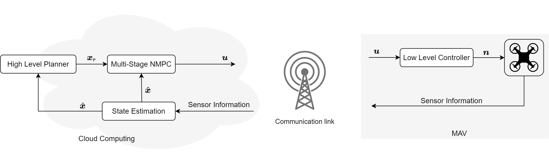
Figure 1: Control scheme of the proposed multi-stage NMPC module, where the control actions $\bm{u}$ based on sensor information is obtained in the cloud, and the low-level controller on the MAV generates motor commands $\bm{n}$. The $\bm{x}$ is state of the system, $\bm{x}_{r}$ is reference value, and $\hat{\bm{x}}$ is estimated state.

Towards designing a computationally efficient controller that predicts further in the future, a theoretical framework for establishing an adaptive prediction horizon was investigated in KRENER201831 , where an Adaptive Horizon Model Predictive Control (AHMPC) has been developed with a varying step prediction horizon that depended on the deviation from the operating point. Thus, the further from the desired states the larger horizons steps were considered. Similarly, to decrease the computation burden of the online optimization, in sun_multi , an event-based Model Predictive Control (MPC) with an adaptive prediction horizon strategy was proposed for the tracking of a unicycle robot. The authors proposed a control scheme that reduces the solving rate when the robot is near the desired location. However, the event-based mechanism relied on the error threshold between the current and reference states that reduced the prediction horizon and the solving frequency and thus could not foresee further in the prediction horizon. A study that fused varying the prediction horizon and time-varying delays was introduced in Arai , where the authors proposed a method for utilizing only resources that are available at a specific time instant by adjusting the prediction horizon properly. The idea of predicting future driving trajectory based on uncertainties for different time horizons with the use of multiple sensors to create a robust and trustworthy prediction system was studied in Huang .

The topic of MAV navigation and path planning is well studied in the related literature lavalle2006planning ; galceran2013survey . Exploration algorithms like the frontier exploration algorithms fentanes2011new , entropy-based algorithms burgard2005coordinated , and information-gain algorithms bhattacharya2013distributed provide a global planning strategy for the MAV, while an additional reactive control layer provides a local obstacle avoidance to prevent collisions with the environment. The most widely used reactive control layer is the artificial potential fields barraquand1992numerical , while another approach that has received attention in the last years is the NMPC kamel2017nonlinear , which has been applied to perform real-time obstacle avoidance for MAVs mansouri2020nmpcmine and disturbance rejection papadimitriou_nmhe . However, all of these methods consider fixed time steps, while in real-life applications and especially in networked enabled MAVs the feature of a time-varying path planning and a corresponding controller that can take into consideration time variations is vital for collision-free navigation.

1.2 Contributions

The first contribution stems from developing a multi-stage NMPC for considering a tree of sampling times while providing collision-free paths for the MAV. The varying sampling time addresses the random delays in the communication link between the MAV and the edge, which results in time uncertainties in the control actions period. In this article, the varying communication delays in the information exchange between the MAV and the controller are addressed by the multi-stage NMPC that is defined by a scenario tree for different sampling times. To the best of our knowledge, no work so far has considered different sampling times in the multi-stage NMPC framework.

The second contribution stems from the introduction of adaptive weights for each scenario of the proposed multi-stage NMPC. The adaptive weights are assigned based on the varying uncertainties of time delays as they are stochastic in the communication link. This approach results in realistic control strategies based on real-world limitations.

The final contribution stems from the overall application on a MAV use-case and the corresponding extensive analysis of the control framework performance under iterative simulations. As it will be presented in the sequel, the proposed control scheme enables collision-free navigation in an obstacle environment, while the generated path distance is reduced in comparison to a fixed sampling time NMPC scheme for path planning.

1.3 Outline

The rest of this article is structured as follows. In Section 2 the research problem is defined, while highlighting the challenges and limitations. Section 3 provides the non-linear model of a MAV, the theoretical control framework and the formulation of the optimization problem. The simulation specifics and results are provided in Section 4, while concluding remarks and future work are discussed in 5.

2 Problem Statement

When a networked control scheme is considered for the control of a MAV the network-induced time delays directly affect the state estimation and the control actions sampling time. Thus this article will propose a multi-stage NMPC that considers the varying sampling times and establish a collision-free path planner. Fig. 1 illustrates the proposed concept while highlighting the overall system architecture. The high-level planner generates references $\bm{x}_{r}$ for the multi-stage NMPC, the controller provides actions $\bm{u}$ for the low-level controller, and the low-level controller feeds the motor commands $\bm{n}=\{\bm{n}_{i},i\in\mathbb{N}^{\geq 4}\}$ to the MAV. Without losing generality, the following assumptions are made:

Assumption 1.

Delays caused by communication are bounded in a specific known range and can be mitigated by different sampling times, as they affect the control action period.

Assumption 2.

The delays affecting the system are transmission delays in the communication link and not processing delays.

Assumption 3.

The transmission delays between the low-level controller and the system are negligible.

Assumption 4.

An NMPC control action $\bm{u}$ that satisfies the constraints for sampling times $t_{s}^{i}$ and $t_{s}^{i+1}$ with $i\in\mathbb{N}$ will satisfy the constraints for all sampling times within $[t_{s}^{i},t_{s}^{i+1}]$.

3 Multi-Stage Nonlinear Model Predictive Control

3.1 MAV Dynamics

In this article, the six Degree of Freedom (DoF) dynamics of a MAV are considered as defined in the body frame (Fig. 2) and modelled by (1):

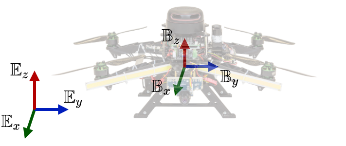
Figure 2: Illustration of the MAV with the attached body fixed frame $\mathbb{B}$ and inertial frame $\mathbb{E}$.

$$\dot{\bm{p}}(t) =\bm{v}(t)$$ (1a)

$$\dot{\bm{v}}(t) =\bm{R}_{x,y}(\theta,\phi)\begin{bmatrix}0\\ 0\\ T\end{bmatrix}+\begin{bmatrix}0\\ 0\\ -g\end{bmatrix}-\begin{bmatrix}A_{x}&0&0\\ 0&A_{y}&0\\ 0&0&A_{z}\end{bmatrix}\bm{v}(t),$$ (1b)

$$\dot{\phi}(t) =\nicefrac{{1}}{{\tau_{\phi}}}(K_{\phi}\phi_{d}(t)-\phi(t)),$$ (1c)

$$\dot{\theta}(t) =\nicefrac{{1}}{{\tau_{\theta}}}(K_{\theta}\theta_{d}(t)-\theta(t)),$$ (1d)

where $\bm{p}=[p_{x},p_{y},p_{z}]^{\top}\in\mathbb{R}^{3}$ is the position vector and $\bm{v}=[v_{x},v_{y},v_{z}]^{\top}\in\mathbb{R}^{3}$ is the vector of linear velocities, $\phi,\theta\in\mathbb{R}\cap[-\pi,\pi]$ are the roll and pitch angles respectively, $\bm{R}_{x,y}$ is the rotation matrix about the $x$ and $y$ axes, $T\in[0,1]\cap\mathbb{R}$ is the mass-normalized thrust, $g$ is the gravitational acceleration, $A_{x},A_{y}$ and $A_{z}\in\mathbb{R}$ are the normalized mass drag coefficients. The low-level control system is approximated by first-order dynamics driven by the reference roll and pitch angles $\phi_{d}$ and $\theta_{d}$ with gains of $K_{\phi},K_{\theta}\in\mathbb{R}^{+}$ and time constants of $\tau_{\phi},\tau_{\theta}\in\mathbb{R}^{+}$ respectively.

3.2 Objective Function

The system states are $\bm{x}=[\bm{p},\bm{v},\phi,\theta]^{\top}$ and the control input is denoted by $\bm{u}=[T,\phi_{d},\theta_{d}]^{\top}$. To obtain a discrete-time dynamical system at time instance $k\in\mathbb{Z}^{+}$, the model expressed by (1) is discretization by the Euler method and with a sampling time of $t_{s}$ as:

$$\bm{x}_{k+1}=f(\bm{x}_{k},\bm{u}_{k}).$$ (2)

The NMPC approach solves a finite-horizon problem at every time instant $k$ with the prediction horizon of $N\in\mathbb{N}^{\geq 2}$. The states and control actions are expressed by $\bm{x}_{k+j+1|k}$, and $\bm{u}_{k+j\mid k}$ respectively for $k+j,\,\forall j\in\{0,1,\dots,N-1\}$ steps ahead from the current time step $k$. The purpose of the NMPC is the tracking of a reference state $\bm{x}_{r}=[\bm{p}_{r},\bm{v}_{r},\phi_{r},\theta_{r}]^{\top}$ by generating the desired thrust $T$ and angles $\phi_{d}$, $\theta_{d}$ commands for the attitude controller, while guaranteeing a safety distance from a priori known obstacles. For this purpose, the finite horizon cost function can be written as:

$$J=\sum_{j=0}^{N-1}\underbrace{\|\bm{x}_{k+j+1|k}-\bm{x}_{r}\|_{\bm{Q}_{x}}^{2}}_{\text{tracking error}}\\ +\underbrace{\|\bm{u}_{k+j+1|k}-\bm{u}_{r}\|_{\bm{Q}_{u}}^{2}}_{\text{actuation}}+\underbrace{\|\bm{u}_{k+j|k}-\bm{u}_{k+j-1|k}\|_{\bm{Q}_{\Delta u}}^{2}}_{\text{smoothness cost}}.$$ (3)

The objective function consists of three terms. The first term ensures the tracking of the desired states $\bm{x}_{r}$ by minimizing the deviation from the current states. The second term, penalizes the deviation from the hover thrust with horizontal roll and pitch, where $\bm{u}_{r}$ is $[g,\,0,\,0]^{\top}$. The last term tracks the aggressiveness of the obtained control actions. In addition, the weights of the objective function’s terms are denoted as $\bm{Q}_{x}\in\mathbb{R}^{8\times 8}$, $\bm{Q}_{u}\in\mathbb{R}^{3\times 3}$ and $\bm{Q}_{\Delta u}\in\mathbb{R}^{3\times 3}$ respectively, which reflect the relative importance of each term.

3.3 Constraints

3.3.1 Cylinder Obstacles

There are different types of obstacles in the surrounding environment, nonetheless all these types of obstacles can be categorized to three types as cylindrical shapes, polytope surfaces, and constrained entrances lindqvist2020non . In this work, we mainly target the cylinder-shaped obstacles. The constraints are defined in parametric form and their positions are fed directly to the NMPC scheme ESmall . When the MAV is outside the obstacle, the associated cost is forced to be zero and for that purpose the function $max(h,0)=[h]_{+}$ is utilized. With the proper selection of the $h$ expression, the constrained area is negative outside the obstacle and positive inside of it.

In case of a cylinder obstacle, the two equations for the safety radius $h_{c}$ and the maximum altitude allowance $h_{z_{max}}$ are defined based on the center position $(x_{obs},y_{obs})$, the radius $r_{obs}$ and the height $z_{obs}$ of the cylinder as follows:

$$h_{c}=r^{2}_{obs}-(x_{k+j|k}-x_{obs})^{2}-(y_{k+j|k}-y_{obs})^{2},$$ (4a)

$$h_{z_{max}}=z_{obs}-z_{k+j|k}.$$ (4b)

By multiplication of (4a) and (4b) the cylinder constraint is defined as:

$$C_{c}=\sum_{j=0}^{N}[h_{c}]_{+}[h_{z}max]_{+}=0.$$ (5)

3.3.2 Input Constraint

Additionally the inputs are constrained within specific boundaries in the following form:

$$\bm{u}_{min}\leq\bm{u}\leq\bm{u}_{max},$$ (6)

where the lower bound $\bm{u}_{min}=[T_{min},\phi_{min},\theta_{min}]^{\top}$ and the upper bound $\bm{u}_{max}=[T_{max},\phi_{max},\theta_{max}]^{\top}$ denote the minimum and maximum values the control actions can take.

3.4 Multi-Stage NMPC

Most of the multi-stage NMPC approaches model the uncertainties by a tree of scenarios lucia2012new . In our case, each scenario is defined based on different sampling times $t_{s}^{i},i\in\{1,\dots,M\}$. To that end, we assume that the sampling time is bounded in range of $[t_{s}^{min},t_{s}^{max}]$, which means that the upper and lower bounds are defined. Based on these bounds and our defined sampling times, each branch of the tree is made as depicted in Fig. 3. Our method varies drastically from the traditional move blocking strategy Morari_move_blocking for model-based control problems that fixes the input for several time steps. In the proposed multi-stage framework, the $\bm{u}$ is the same in all branches of the tree, which means that the obtained control action can satisfy all the sampling times.

Figure 3: Illustration of the scenario tree with different sampling times.

The multi-stage NMPC objective function based on the classic NMPC cost (3) denoted here as $J_{i}$ for the $M\in\mathbb{N}$ scenarios can be formulated as follows:

$$\!\min_{\{u_{k+j\mid k}\}^{N-1}_{j=0}} \sum_{i=1}^{M}\omega_{i}J_{i}\quad\forall i\in\{1,\dots,M\}$$ (7a)

s.t. $$\bm{x}_{k+j+1\mid k}=f_{i}(\bm{x}_{k+j\mid k},\bm{u}_{k+j\mid k}),$$ (7b)

$$\text{Constraints}\leavevmode\nobreak\ \eqref{eq:cylinderconstraints},\eqref{eq:input_constraints}.$$ (7c)

To consider uncertainties in delays, the term $\omega_{i}$ defines the weight of each scenario objective function of the multi-stage NMPC. The $\omega_{i}$ is updated based on the probability of the delays. To estimate the $\omega_{i}$ adaptive term, the network transmission delays are stored in a finite buffer as follows:

$$\bm{t_{d}}=\{(t_{d,1},\dots,t_{d,l}),l\in\{k-(n_{max}-1),\dots,k\}\},$$ (8)

where $t_{d}$ is a single communication delay and $n_{max}$ is the limited window size of stored network delays.Furthermore, it is assumed that the communication delays that affect the control framework are following a Gamma distribution. Initially, the shape $\alpha$ and scale parameters $\beta$ of the Gamma distribution are calculated from the mean $\mu$ and the standard deviation $\sigma$ of set $\bm{t_{d}}$ as:

$$\alpha=\frac{\mu^{2}}{\sigma^{2}},\leavevmode\nobreak\ \leavevmode\nobreak\ \beta=\frac{\sigma^{2}}{\mu}.$$ (9)

The probability of a single random delay $t^{i}_{d}$ from a Gamma distribution with parameters $\alpha,\beta$ falls in the interval $[0,t_{d}]$ and is given from the Cumulative Distribution Function (CDF) mathematicshandbook as:

$$G(t_{d};\alpha,\beta)=\frac{1}{\beta^{\alpha}\Gamma(\alpha)}\int_{0}^{t_{d}}x^{a-1}e^{\frac{-x}{\beta}}dx,$$ (10)

where $\Gamma(\cdot)$ is the Gamma function mathematicshandbook . Based on the obtained probabilities for the selected span of delays, the $\omega_{i}$ for each branch of the tree is derived as follows:

$$\omega_{i}=\begin{cases}G(t_{d}^{1};\alpha,\beta)&\,\text{if }i=1\\ G(t_{d}^{i};\alpha,\beta)-G(t_{d}^{i-1};\alpha,\beta),&\,\text{if }i\in\{2,\dots,M\}\end{cases}$$ (11)

At each time step, the multi-stage NMPC generates an optimal sequence of control actions $\bm{u}_{k|k}^{\star}$, $\dots$, $\bm{u}_{k+N-1|k}^{\star}$, and only the first control action $\bm{u}_{k|k}^{\star}$ is applied based on a zero-order hold element as $\bm{u}(t)=\bm{u}_{k|k}^{\star}$ for $t\in[kt_{s},(k+1)t_{s}]$.

The developed multi-stage NMPC with 3D collision avoidance constraints, is solved with Proximal Averaged Newton-type method for Optimal Control (PANOC) sathya2018embedded to guarantee a real-time performance. In the related literature for solving the multi-stage NMPC optimization problem, algorithmic procedures are used Lucia2013 relying on solving each of the scenarios independently until the solutions converge and the constraints are satisfied. To this extent, a large optimization problem can be solved in a reasonable amount of time. In contrast, in this article, we attempt a one-shot solution by taking advantage of the PANOC solving capabilities. Thus, a single cost function is built for the $M$ discrete scenarios, under a set of constraints. In such a manner, the solution of the multi-stage NMPC problem satisfies all the scenarios and constraints.

The simulation trials were running on a single core to solve the optimization problem and they performed in a personal computer with an Intel(R) Core(TM) i7-8550U @ $1.8\,\mathrm{Ghz}$ processor with $16\,\mathrm{GB}$ of RAM.

4 Results

4.1 Simulation Setup

Out of the numerous simulations, three representative cases are selected to prove the performance of the proposed control scheme. For consistent results, data of delays generated from a Gamma distribution $\Gamma(\alpha,\beta)$ with shape factor $\alpha=12$ and scale factor $\beta=0.015$ is used for all the simulation trials. During the simulations, the eight states of the MAV considered measurable and were updated based on the communication delays i.e. for the duration of a delay, the cloud computing controller has no knowledge of the states’ evolution and the MAV maintains the last control input, while in MAV’s side (Fig. 1), no delay is considered between low-level controller and the platform.

Two environments and three simulation trials are chosen to demonstrate the main attributes of the proposed control framework. The first environment includes a single large cylinder obstacle, where the performance of the multi-stage NMPC is compared with the standard NMPC under the presence of communication delays for navigating to a desired location, while the path is obstructed by the cylinder. By standard NMPC is defined the solution of (7a) for $M=1$, $\omega_{i}=1$ and solved at nominal $t_{s}$. It should be noted that only the desired point is provided for the multi-stage NMPC and NMPC and the controller is generating collision free paths. For the second and the third simulation trials, a more complex environment is selected with three cylinders of different sizes. Same as in the first case, we compare the performance of the multi-stage NMPC and the NMPC under the presence of varying communication delays, while trying to reach a desired location avoiding collision with the three cylinders. Finally, we compare the performance of the multi-stage NMPC and the NMPC in the same environment without communication delays to demonstrate the better path planning of the proposed controller with a collision avoidance capability due to the consideration of higher sampling times.

Fig. 4 shows the delay data during the single obstacle simulation trial (Top), while inside the same illustration the histogram of the complete delays data-set is presented. Furthermore, the calculated probabilities for specific delays in logarithmic scale are given in Fig. 4 (Bottom).

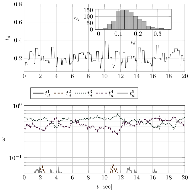
Figure 4: Communication delays of the single cylinder obstacle simulation trial and histogram of the complete data of delays (Top). Calculated weights $\omega_{i}$ of the same simulation trial (Bottom).

The parameters of the non-linear MAV model are the mass $m=1\,\mathrm{kg}$, the gravitational acceleration $g=9.81\,\mathrm{m/s^{2}}$, the mass normalized drag coefficients $A_{x},A_{y}=0.1$ and $A_{z}=0.2$, and the time constants $t_{\phi},t_{\theta}=0.5\,\mathrm{sec}$ with gains $K_{\phi},K_{\theta}=1$. The prediction horizon $N$ is 40, the nominal sampling time is $t_{s}=0.05\,\mathrm{sec}$, while the multi-stage NMPC considers sampling times scenarios in seconds of $\bm{t_{s}}=[0.05,0.07,0.1,0.2,0.33]$. The roll and pitch angles are constrained within $[-\pi/18\leq\phi,\theta\leq\pi/18],\ \mathrm{rad}$. On account of the different simulation environments, the tuning weight parameters of the controller $\bm{Q}_{x}$ and $\bm{Q}_{u}$ vary among the simulations and the numerical values will be given in the sequel.

4.2 Single Cylinder Obstacle under Communication Delays

For the first case, as depicted in Fig. 5 a cylinder obstacle of radius $1.5\,\mathrm{m}$ and height $10\,\mathrm{m}$ located at $x,y\leavevmode\nobreak\ (0,6)\,\mathrm{m}$ is considered, while it is obstructing the straight path from the initial position $\bm{p}_{\text{init}}=[0,0,0],\ \mathrm{m}$ to the desire goal position $\bm{p}_{\text{goal}}=[0,9,1],\ \mathrm{m}$. For a better illustration, the obstacle in Fig. 5 is limited in the range of 0 to $1.25\,\mathrm{m}$. The weights of the states are $\bm{Q}_{x}=\text{diag}[6,6,20,50,50,10,20,20]$, while the control action weights are $\bm{Q}_{u}=\text{diag}[20,20,20]$ and for the input rate of change are $\bm{Q}_{\Delta u}=\text{diag}[40,65,65]$.

In Fig 5 the multi-stage NMPC successfully regulates the control inputs and the MAV navigates to the desired location despite the effect of delays. On the other hand, with the same weights and delays the NMPC stops in a local minimal at approximately $\bm{p}=[0,5,1],\mathrm{m}$. Since, the multi-stage NMPC considers higher sampling times, at most $t_{s}^{5}=0.33\,\mathrm{sec}$ with the prediction horizon of 40 steps it can predict 13.2 seconds in the future when compared to the minimum sampling time scenario of $t_{s}^{1}=0.05$ seconds, which predicts at most up to the next 2 seconds.

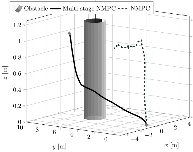
Figure 5: Performance comparison of the multi-stage NMPC versus NMPC navigation under the effect of delays in presence of a cylinder obstacle

Finally, for the first case the control actions roll pitch and thrust for both tested controllers is presented in Fig. 6. It can be noticed that the multi-stage NMPC starts aggressively in the beginning but as approaches the desired location the roll and pitch angles are getting smoother. On the other hand, the NMPC almost immediately falls into shacking issues due to the delays, something that could be observed in the Fig. 5 as well. Both the multi-stage and classic NMPC provide solutions that do not violate the given constraints denoted by light-grey dashed line in Fig. 6. For the thrust, the NMPC is observed to be more aggressive when compared to the multi-stage NMPC but both controllers successfully manage to regulate the height at $1\,\mathrm{m}$.

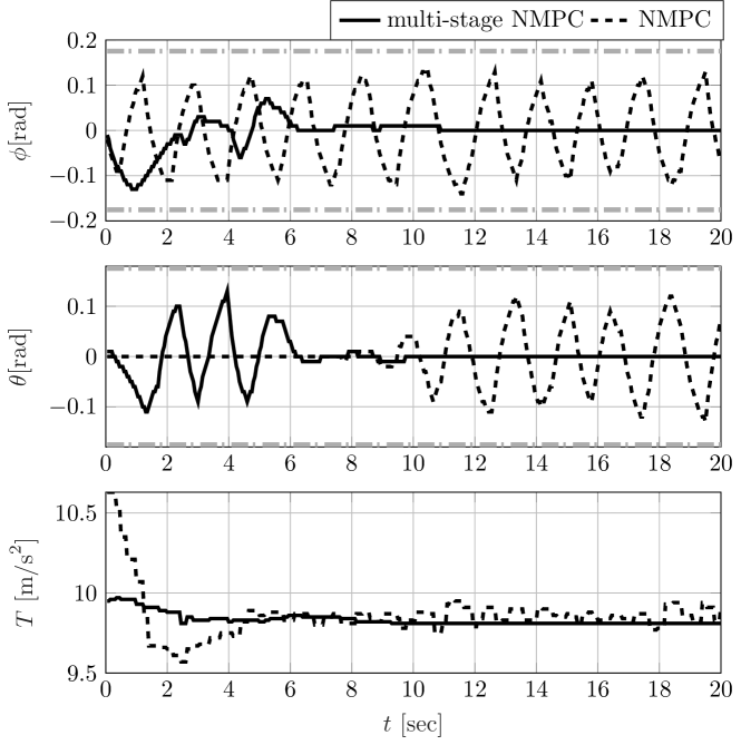
Figure 6: Control action responses of roll, pitch and Thrust under the effect of communication delays in presence of a cylinder obstacle for multi-stage NMPC and NMPC

4.3 Multiple Cylinder Obstacles under Communication Delays

For the second case three cylinder obstacles of radius 0.25, 0.4 and $0.5\,\mathrm{m}$ are located at $x,y\leavevmode\nobreak\ (3.5,1.5)\leavevmode\nobreak\ (2.8,3.0)\leavevmode\nobreak\ \text{and}\leavevmode\nobreak\ (4.3,4.1)\mathrm{m}$ respectively of $10\,\mathrm{m}$ height obstructing MAV’s path from the initial position $\bm{p}_{init}=[3.2,0,0]\,\mathrm{m}$ to the goal position $\bm{p}_{goal}=[3.2,5,1]\,\mathrm{m}$. As in the previous cases and for visualization purposes, the $z$-axis in Fig. 7, is limited between 0 and $1.25\,\mathrm{m}$. The tuning of the controllers is $\bm{Q}_{x}=\text{diag}[12.5,12.5,20,30,30,10,20,20]$, while the control input weights are $\bm{Q}_{u}=\text{diag}[20,20,20]$ and the weight of the smoothness term is $\bm{Q}_{\Delta u}=\text{diag}[40,165,165]$.

Fig. 7 illustrates the path followed by the multi-stage NMPC (solid line) and the NMPC (dashed line). Both controllers manage to navigate to the goal location. The multi-stage NMPC path is characterized to be more smooth compared to the NMPC path, something that can be observed by the smaller changes in $x,y$ and $z$ positions, as well as in the control actions in Fig 8. The multi-stage controller manages to regulate the height steadily to the reference point in contrast to the NMPC, which overshoots and undershoots in the beginning mainly due to the existence of the delays.

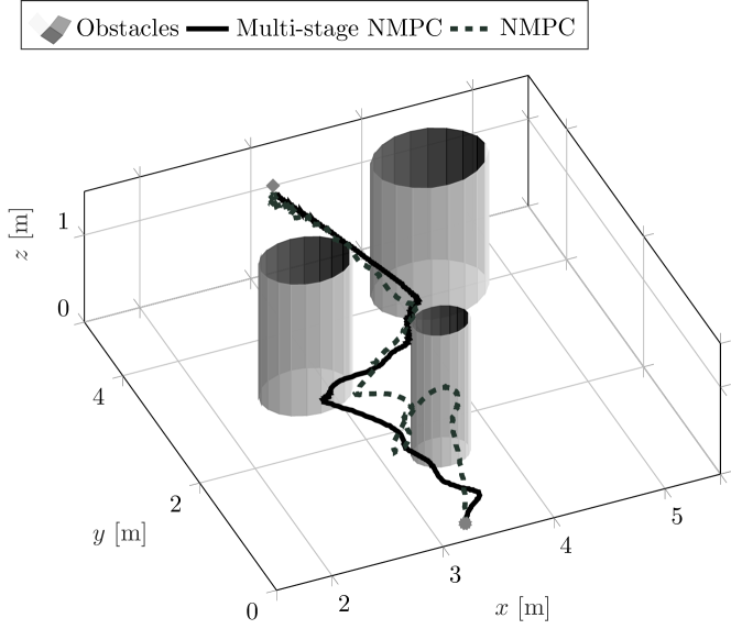
Figure 7: Performance comparison of the multi-stage NMPC versus NMPC navigation under the effect of delays in presence of multiple cylinder obstacles

The roll, pitch and thrust commands of the second simulation are given in Fig. 8. For the NMPC the $\phi$ and $\theta$ are oscillating in the range $\pm 0.1\,\mathrm{rad}$ for almost the entire time response. In contrast, the multi-stage NMPC appears to be affected less by the communication delays and results in much smoother control actions. It is noticeable that NMPC even if it manages to drive the MAV to the final position its path response is more aggressive as the MAV drifts from the expected position due to the delays. On the other hand, the multi-stage NMPC results in a much smoother navigation path. This can be also identified in the altitude commands, where the control signal of the NMPC changes abruptly at the beginning of the response and this is causing the platform to overshoot and undershoot in the height response as well.

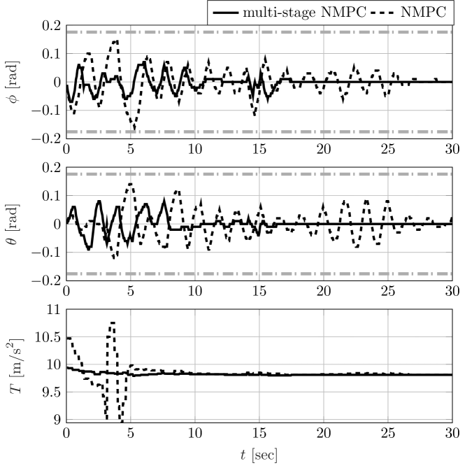
Figure 8: Multi-stage NMPC and NMPC control actions roll, pitch and thrust under the effect of delays in presence of multiple cylinder obstacles.

4.4 Multiple Cylinder Obstacles without Communication Delays

For the final test, the simulation tuning and constraints are identical to the second simulation, while no time delay is considered ($t_{d}=0$). The multi-stage probability is kept constant at $\bm{\omega}_{i}=[0.05,0.15,0.45,0.30,0.05]$ for the sampling times of $\bm{t}_{s}=[0.05,0.07,0.1,0.2,0.33],\mathrm{sec}$. Thus, the higher the sampling time is the further in the future we predict for achieving an improved path planning. As depicted in Fig. 9, under the absence of time delays both controllers successfully reach to the destination point with smooth maneuvers avoiding the obstacle from shorter path in comparison to the previous simulation. Even in this case, as it is presented in Table 1, the multi-stage NMPC results in a shorter path compared to the NMPC, while this time the difference between the two navigation performances is smaller.

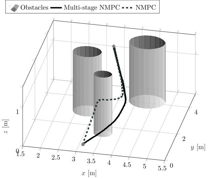
Figure 9: Performance comparison of the multi-stage NMPC versus the NMPC navigation for $t_{d}=0$ in presence of multiple cylinder obstacles

Fig. 10 presents the $\phi,\theta$ and $T$ actions of the last simulation under zero communication delays. The multi-stage NMPC appears to be more resilient to the control input changes and thus resulting to smaller variations from the hover position. In comparison to Fig. 8 from the previous simulation, all the signal responses are smooth, indicating the intense effect of the delays on the aerial platform.

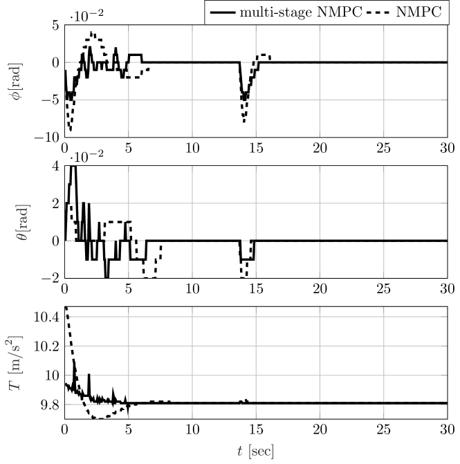
Figure 10: Multi-stage NMPC and NMPC control actions of roll, pitch and thrust for $t_{d}=0$ in presence of multiple cylinder obstacles.

Finally, in Tables 1 and 2 a comparison of the path length and mean computation time between the proposed multi-stage NMPC is presented. For all the simulation trials, the distance from the initial point to the goal point is shorter for the multi-stage NMPC. As far as the computation time is concerned, the NMPC has a lower mean computation time as expected due to the smaller size of the optimization problem, but it must be highlighted that the NMPC fails to overcome the obstacle in the first simulation and it has an overall lower performance in the second and third simulation. Furthermore, the computation time of the multi-stage NMPC is fast enough since typical path planners operate at a sampling rate of $50\,\mathrm{ms}$.

Table 1: Comparison of the path length between the proposed multi-stage NMPC and the path from NMPC.

[b] Scenario Simulation 1 Simulation 2 Simulation 3 NMPC 6.45¹ [m] 8.99 [m] 5.75 [m] Multi-stage NMPC 9.75 [m] 6.18 [m] 5.46 [m]

• Failed to reach final destination

Table 2: Comparison of the average computation time between the proposed multi-stage NMPC and the classic NMPC.

Scenario	Simulation 1	Simulation 2	Simulation 3
NMPC	15.1 [ms]	4.3 [ms]	1.6 [ms]
Multi-stage NMPC	20.5 [ms]	48.1 [ms]	19.7 [ms]

5 Conclusions

This article proposed a novel multi-stage NMPC framework for collision-free navigation of MAV under the effect of time delays in the communication network. The multi-stage NMPC scenarios were based on different sampling times and varying weights derived from the communication delays. The proposed control scheme was evaluated under multiple simulations for different numbers of obstacles and variable communication delays. More specifically, the multi-stage was able to compensate for the network delays and navigate to the final point avoiding the cylinder obstacle that obstructed its path, while the classic NMPC failed to reach the desired point. The navigation in the environment with three obstacles without delays is considered, where the multi-stage NMPC presented a smoother motion and fewer fluctuations in the control actions compared to the classic NMPC, while with both controllers the MAV successfully navigated from the initial point to the final point. For all the aforementioned cases, the generated paths were shorter compared to the fixed sampling rate NMPC. Lastly, even tough the mean computation time of the multi-stage controller was higher compared to the NMPC, it is lower than shortest sampling time and the multi-stage control shows better performance in generating collision free paths. Further studies will focus on the stability analysis and experimental evaluation with a 5G enabled MAV platform for collision-free navigation in urban environments.

6 Declarations

Funding

This work has been partially funded by the European Union Horizon 2020 Research and Innovation Programme under the Grant Agreement No. 869379 illuMINEation.

Conflict of interest/Competing interests

The authors declare that they have no conflict of interest.

Availability of data and material

Not applicable.

Code availability

Not applicable.

Author’s contributions

Andreas Papadimitriou: Conceptualization, Methodology, Software, Validation, Formal analysis, Investigation, Writing - Original Draft, Visualization
Hedyeh Jafari: Conceptualization, Methodology, Validation, Resources, Writing - Original Draft
Sina Sharif Mansouri: Conceptualization, Methodology, Software, Validation, Resources, Writing - Original Draft, Visualization, Supervision, Project administration
George Nikolakopoulos: Funding acquisition, Supervision

Ethics approval

Not applicable.

Consent to participate

Not applicable.

Consent for publication

Not applicable.

References

- \bibcommenthead
- (1) Mansouri, S.S., Kanellakis, C., Fresk, E., Kominiak, D., Nikolakopoulos, G.: Cooperative coverage path planning for visual inspection. Control Engineering Practice 74, 118–131 (2018)
- (2) Mansouri, S.S., Kanellakis, C., Kominiak, D., Nikolakopoulos, G.: Deploying MAVs for autonomous navigation in dark underground mine environments. Robotics and Autonomous Systems, 103472 (2020)
- (3) Hallermann, N., Morgenthal, G.: Visual inspection strategies for large bridges using unmanned aerial vehicles (uav). In: Proc. of 7th IABMAS, International Conference on Bridge Maintenance, Safety and Management, pp. 661–667 (2014)
- (4) Ullah, H., Nair, N.G., Moore, A., Nugent, C., Muschamp, P., Cuevas, M.: 5g communication: an overview of vehicle-to-everything, drones, and healthcare use-cases. IEEE Access 7, 37251–37268 (2019)
- (5) Nikolakopoulos, G., Panousopoulou, A., Tzes, A.: Experimental controller tuning and qos optimization of a wireless transmission scheme for real-time remote control applications. Control Engineering Practice 18(3), 333–346 (2008)
- (6) Holtorf, F., Mitsos, A., Biegler, L.T.: Multistage nmpc with on-line generated scenario trees: Application to a semi-batch polymerization process. Journal of Process Control 80, 167–179 (2019)
- (7) Alaimo, A., Artale, V., Milazzo, C., Ricciardello, A.: Comparison between euler and quaternion parametrization in uav dynamics. In: AIP Conference Proceedings, vol. 1558, pp. 1228–1231 (2013). American Institute of Physics
- (8) Alaimo, A., Artale, V., Milazzo, C., Ricciardello, A., Trefiletti, L.: Mathematical modeling and control of a hexacopter. In: Unmanned Aircraft Systems (ICUAS), 2013 International Conference On, pp. 1043–1050 (2013). IEEE
- (9) Krener, A.J.: Adaptive horizon model predictive control. IFAC-PapersOnLine 51(13), 31–36 (2018). https://doi.org/10.1016/j.ifacol.2018.07.250. 2nd IFAC Conference on Modelling, Identification and Control of Nonlinear Systems MICNON 2018
- (10) Sun, Z., Xia, Y., Dai, L., Campoy, P.: Tracking of unicycle robots using event-based mpc with adaptive prediction horizon. IEEE/ASME Transactions on Mechatronics 25(2), 739–749 (2020)
- (11) Arai, H., Uchimura, Y.: Model predictive control with variable prediction horizon for a system including time-varying delay. In: IECON 2019 - 45th Annual Conference of the IEEE Industrial Electronics Society, vol. 1, pp. 3281–3286 (2019)
- (12) Huang, X., McGill, S.G., Williams, B.C., Fletcher, L., Rosman, G.: Uncertainty-aware driver trajectory prediction at urban intersections. In: 2019 International Conference on Robotics and Automation (ICRA), pp. 9718–9724 (2019)
- (13) LaValle, S.M.: Planning Algorithms vol. 9780521862059, (2006). https://doi.org/10.1017/CBO9780511546877
- (14) Galceran, E., Carreras, M.: A survey on coverage path planning for robotics. Robotics and Autonomous Systems 61(12), 1258–1276 (2013)
- (15) Fentanes, J.A.P., Alonso, R.F., Zalama, E., García-Bermejo, J.G.: A new method for efficient three-dimensional reconstruction of outdoor environments using mobile robots. Journal of Field Robotics 28(6), 832–853 (2011)
- (16) Burgard, W., Moors, M., Stachniss, C., Schneider, F.E.: Coordinated multi-robot exploration. IEEE Transactions on Robotics 21(3), 376–386 (2005)
- (17) Bhattacharya, S., Michael, N., Kumar, V.: In: Martinoli, A., Mondada, F., Correll, N., Mermoud, G., Egerstedt, M., Hsieh, M.A., Parker, L.E., Støy, K. (eds.) Distributed Coverage and Exploration in Unknown Non-convex Environments, pp. 61–75. Springer, Berlin, Heidelberg (2013). https://doi.org/10.1007/978-3-642-32723-0_5
- (18) Barraquand, J., Langlois, B., Latombe, J.-C.: Numerical potential field techniques for robot path planning. IEEE transactions on systems, man, and cybernetics 22(2), 224–241 (1992)
- (19) Kamel, M., Alonso-Mora, J., Siegwart, R., Nieto, J.: Nonlinear model predictive control for multi-micro aerial vehicle robust collision avoidance. arXiv preprint arXiv:1703.01164 (2017)
- (20) Mansouri, S.S., Kanellakis, C., Fresk, E., Lindqvist, B., Kominiak, D., Koval, A., Sopasakis, P., Nikolakopoulos, G.: Subterranean MAV navigation based on nonlinear MPC with collision avoidance constraints. IFAC-PapersOnLine (2020)
- (21) Papadimitriou, A., Jafari, H., Mansouri, S.S., Nikolakopoulos, G.: External force estimation and disturbance rejection for micro aerial vehicles. Expert Systems with Applications 200, 116883 (2022). https://doi.org/10.1016/j.eswa.2022.116883
- (22) Lindqvist, B.: Non-linear mpc based navigation for micro aerial vehicles in constrained environments. In: European Control Conference 2020, May 12-15, St. Petersburg, Russia. (2020)
- (23) Small, E., Sopasakis, P., Fresk, E., Patrinos, P., Nikolakopoulos, G.: Aerial navigation in obstructed environments with embedded nonlinear model predictive control. In: 2019 18th European Control Conference (ECC), pp. 3556–3563 (2019). https://doi.org/10.23919/ECC.2019.8796236
- (24) Lucia, S., Finkler, T., Basak, D., Engell, S.: A new robust nmpc scheme and its application to a semi-batch reactor example. IFAC Proceedings Volumes 45(15), 69–74 (2012)
- (25) Cagienard, R., Grieder, P., Kerrigan, E.C., Morari, M.: Move blocking strategies in receding horizon control. In: 2004 43rd IEEE Conference on Decision and Control (CDC) (IEEE Cat. No.04CH37601), vol. 2, pp. 2023–20282 (2004). https://doi.org/10.1109/CDC.2004.1430345
- (26) Lennart Råde, B.W.: Mathematics Handbook for Science and Engineering. Springer, Berlin, Heidelberg (2004). https://doi.org/10.1007/978-3-662-08549-3
- (27) Sathya, A.S., Sopasakis, P., Van Parys, R., Themelis, A., Pipeleers, G., Patrinos, P.: Embedded nonlinear model predictive control for obstacle avoidance using panoc. In: Proceedings of the 2018 European Control Conference (2018)
- (28) Lucia, S., Subramanian, S., Engell, S.: Non-conservative robust nonlinear model predictive control via scenario decomposition. In: 2013 IEEE International Conference on Control Applications (CCA), pp. 586–591 (2013)