Modules for Experiments in Stellar Astrophysics (MESA):
Time-Dependent Convection, Energy Conservation,
Automatic Differentiation, and Infrastructure

Abstract

We update the capabilities of the open-knowledge software instrument Modules for Experiments in Stellar Astrophysics (MESA). The new auto_diff module implements automatic differentiation in MESA, an enabling capability that alleviates the need for hard-coded analytic expressions or finite difference approximations. We significantly enhance the treatment of the growth and decay of convection in MESA with a new model for time-dependent convection, which is particularly important during late-stage nuclear burning in massive stars and electron degenerate ignition events. We strengthen MESA’s implementation of the equation of state, and we quantify continued improvements to energy accounting and solver accuracy through a discussion of different energy equation features and enhancements. To improve the modeling of stars in MESA  we describe key updates to the treatment of stellar atmospheres, molecular opacities, Compton opacities, conductive opacities, element diffusion coefficients, and nuclear reaction rates. We introduce treatments of starspots, an important consideration for low-mass stars, and modifications for superadiabatic convection in radiation-dominated regions. We describe new approaches for increasing the efficiency of calculating monochromatic opacities and radiative levitation, and for increasing the efficiency of evolving the late stages of massive stars with a new operator split nuclear burning mode. We close by discussing major updates to MESA’s software infrastructure that enhance source code development and community engagement.

1 Introduction

A resurgence of stellar astrophysics research is being fueled by the transformative capabilities in space- and ground-based hardware instruments providing an unprecedented volume of high-quality measurements of stars, significantly strengthening and extending the observational data upon which stellar astrophysics ultimately rests (National Research Council, 2021). Examples include:

Several individual stars at redshifts of $\simeq$ 1 have been discovered by temporary magnification factors of $\simeq$ 1000 from microlensing (Kelly et al., 2018; Rodney et al., 2018; Chen et al., 2019). A more persistent and highly magnified star at a redshift of 6.2 has also been discovered with the Hubble Space Telescope (Welch et al., 2022a) by a fortuitous alignment with a foreground galaxy cluster lens caustic (Windhorst et al., 2018). The infrared instruments aboard the James Webb Space Telescope (Gardner et al., 2006; Beichman et al., 2012; Artigau et al., 2014; Rieke et al., 2015; Labiano et al., 2021) will search for confirmation and spectral classification of this distant star (Welch et al., 2022b) to define its place on the Hertzsprung–Russell Diagram (HRD), assess how galaxies evolve from their formation (Zackrisson et al., 2011; Robertson, 2021), observe the formation of stars (Senarath et al., 2018; Boquien & Salim, 2021), and measure the properties of stellar-planetary systems including the Solar System (Sarkar & Madhusudhan, 2021; Patapis et al., 2022).

In the late 2020s, kilometer-scale gravitational wave detectors such as Advanced Laser Interferometer Gravitational Observatory (LIGO Scientific Collaboration et al., 2015), Advanced Virgo (Acernese et al., 2015) and Kamioka Gravitational Wave Detector (Akutsu et al., 2021) will routinely detect tens of binary neutron-star mergers with kilonovae annually (Abbott et al., 2018), probe how kilonova r-process nucleosynthetic yields vary with environment (e.g., Barnes et al., 2021), and assess the populations that contribute to the stellar black hole mass distribution, including the presence of any gaps in the distribution (Perna et al., 2019; Zevin et al., 2021; Renzo et al., 2020, 2021; Mandel & Broekgaarden, 2022).

The next core-collapse supernova in the Milky Way or its satellites will be a unique opportunity to observe the explosion of a star. The SuperNova Early Warning System is a global network of neutrino experiments sensitive to supernova neutrinos (Al Kharusi et al., 2021) that includes multi-kiloton detectors such as KamLAND (Araki et al., 2005), Borexino (Borexino Collaboration et al., 2018, 2020), SNO+ (Andringa et al., 2016), Daya Bay (Guo et al., 2007), SuperKamiokande (Simpson et al., 2019), and the upcoming HyperKamiokande (Abe et al., 2016), DUNE (Acciarri et al., 2016) and JUNO (JUNO Collaboration, 2022). Searching for pre-supernova neutrinos is ongoing, and of interest as they allow tests of stellar and neutrino physics (e.g., Kosmas et al., 2022) and enable an early alert of an impending core-collapse supernova to the electromagnetic and gravitational wave communities (Beacom & Vogel, 1999; Vogel & Beacom, 1999; Mukhopadhyay et al., 2020; Al Kharusi et al., 2021).

Sky surveys that probe ever-larger areas of the dynamic sky and ever-fainter transient sources include the Imaging X-ray Polarimetry Explorer (Soffitta et al., 2021), the Compton Spectrometer and Imager (Tomsick & COSI Collaboration, 2022), eROSITA (Predehl et al., 2021), Gaia (Gaia Collaboration et al., 2016, 2018, 2021), the Sloan Digital Sky Survey (York et al., 2000; Abdurro’uf et al., 2022), the All-Sky Automated Survey for Supernovae (Chen et al., 2022), Pan-STARRS1 (Flewelling et al., 2020), the Zwicky Transient Factory (Bellm et al., 2019; Dhawan et al., 2022), Gattini-IR (Moore et al., 2016), and the Nancy Grace Roman Space Telescope (Akeson et al., 2019). Roman will measure proper motions of stars several magnitudes fainter than the Gaia mission (Brandt et al., 2021; Dorn-Wallenstein et al., 2021), which is sufficient to probe the main sequence turnoff to distances of $\simeq$ 10 kpc and red giants throughout the Galactic halo (Spergel et al., 2015).

Wide-field spectroscopic surveys in the coming decade will resolve stellar populations and the Milky Way’s structure (Bolton et al., 2019) at facilities such as Gaia DR3 (Gaia Collaboration et al., 2021), SDSS-V (Kollmeier et al., 2017), FOBOS (Bundy et al., 2019), Maunakea Spectroscopic Explorer (Marshall et al., 2019), and SpecTel (Ellis & Dawson, 2019). For example, FOBOS is a next-generation spectroscopic facility at the W.M. Keck Observatory that will provide multi-epoch, high-multiplex, and deep spectroscopic follow-up of panoramic deep-imaging surveys.

The Vera C. Rubin Observatory will conduct a multicolor optical survey of the Southern Hemisphere sky, the Legacy Survey of Space and Time (LSST Science Collaboration et al., 2017; Ivezić et al., 2019), to probe dark energy and dark matter (Sánchez et al., 2021; Zhang et al., 2022), explore the transient optical sky (Bianco et al., 2022; Li et al., 2022; Raiteri et al., 2022; Hernitschek & Stassun, 2022; Andreoni et al., 2022; Bellm et al., 2022), and build a catalog of solar system objects with an order of magnitude more objects (LSST Solar System Science Collaboration et al., 2020; Schwamb et al., 2021).

The TESS mission (Ricker et al., 2016) is providing systematic measurements of the radii, masses, and ages of 200,000 individual stars sampled at a 2 minute cadence to open a new era of stellar variability exploration (e.g., Huang et al., 2018; Ball et al., 2018; Dragomir et al., 2019; Wang et al., 2019). Within the next decade, the Planetary Transits and Oscillations of Stars mission (PLATO; Rauer et al., 2014) will search for planetary transits across up to one million stars, characterize rocky extrasolar planets around yellow dwarf stars, subgiant stars, and red dwarf stars (Montalto et al., 2021), and investigate the seismology of stars (Miglio et al., 2017; Cunha et al., 2021; Nascimbeni et al., 2022).

In partnership with this ongoing explosion of activity in stellar astrophysics, revolutionary advances in software infrastructure, computer processing power, data storage capability, and open-knowledge software instruments are transforming how stellar theory, modeling, and simulations interact with experiments and observations. Examples include Astropy (Astropy Collaboration et al., 2018, 2022), Athena++ (Stone et al., 2020; Jiang, 2021), Castro (Almgren et al., 2020), Dedalus (Burns et al., 2020), emcee (Foreman-Mackey et al., 2013), Flash-X (Dubey et al., 2022), GYRE (Townsend & Teitler, 2013; Townsend et al., 2018), MAESTROeX (Fan et al., 2019), MESA2Hydro (Joyce et al., 2019), MSG (Townsend & Lopez, 2022), Phantom (Price et al., 2018), PHOEBE (Conroy et al., 2020), Starlib (Sallaska et al., 2013), TARDIS (Vogl et al., 2019), TULIPS (Laplace, 2022), and yt (Turk et al., 2011).

The previous Modules for Experiments in Stellar Astrophysics software instrument papers (Paxton et al. 2011, MESA I; Paxton et al. 2013, MESA II; Paxton et al. 2015, MESA III; Paxton et al. 2018, MESA IV; Paxton et al. 2019, MESA V), as well as this one, describe new capabilities and limitations of MESA while also comparing to other available numerical or analytic results. We do not fully explore the science implications in this software instrument paper. The scientific potential of these new capabilities will be unlocked by future efforts of the MESA research community.

This MESA VI software instrument paper is organized as follows. Section 2 describes the implementation of automatic differentiation and §3 introduces a new model for time dependent convection. Section 4 describes improvements to MESA’s implementation of the equation of state (EOS) and §5 discusses treatments of the energy equation. Section 6 describes treatments of the stellar atmosphere and §7 introduces new models of starspots and a superadiabatic convection. Section 8 reports improvements to the opacities, §9 to the element diffusion coefficients, §10 to the nuclear physics, and §11 to the physical constants. Section 12 discusses MESA’s infrastructure. Finally, §13 summarizes MESA VI.

Important symbols are defined in Table 1. Acronyms are defined in Table 1. Components of MESA, such as modules and routines, are in typewriter font e.g., tdc.

Table 1: Important symbols.

Name	Description	Appears
$a$	Radiation constant	7.2
$\mathcal{A}$	$4\pi r^{2}$   Area of face	3
$c$	Speed of light in a vacuum	8
$D$	Element diffusion coefficient	9
$e$	Specific internal energy	4
$E$	Energy	5
$f_{\text{spot}}$	Filling factor	7.1
$g$	Gravitational acceleration	6
$G$	Gravitational constant	6
$h$	Pressure scale height	3
$\kappa$	Opacity	6
$\lambda$	Reaction rate	10
$k_{\mathrm{B}}$	Boltzmann constant	9
$L$	Luminosity	3
$m$	Mass coordinate	3
$M$	Stellar mass	3
$n$	Number density	9
$N_{\mathrm{\!A}}$	Avogadro number	8
$P$	Pressure	3
$Q$	Thermal expansion	3
$r$	Radial coordinate	6
$R$	Stellar radius	6
$\rho$	Mass density	3
$s$	Specific entropy	4
$\sigma$	Stefan-Boltzmann constant	3
$t$	Time	3
$T$	Temperature	3
$u$	Velocity	5
$w$	Turbulent velocity	3
$x_{\text{spot}}$	Temperature contrast	7.1
X	Hydrogen mass fraction	3
Y	Helium mass fraction	3
$\mathcal{Y}$	Superadiabaticity $\nabla$$-$$\nabla_{{\rm ad}}$	3
$Z$	Charge	9
Z	Metal mass fraction	9

$a_{e}$ & Electron spacing (4$\pi n_{e}$/3)^-1/3 9 $\alpha$ Convective flux parameter 3 $\alpha_{D}$ Convective flux parameter 3 $\alpha_{r}$ Convective flux parameter 3 $\alpha_{P_{t}}$ Convective flux parameter 3 $c_{P}$ Specific heat at constant pressure 3 $\alpha_{t}$ Convective flux parameter 3 $c_{V}$ Specific heat at constant volume $\partial e/\partial T|_{\rho}$ 5 $\delta t$ Numerical time step 5 $dm$ Mass of cell 5 $\epsilon$ Energy generation rate 5 $\epsilon_{\mathrm{grav}}$ Gravitational heating rate 4 $\epsilon_{\mathrm{nuc}}$ Nuclear energy generation rate 10 $\epsilon_{q}$ Viscous heating rate 3 $e_{t}$ Specific kinetic energy of turbulence 3 $\Gamma$ Efficiency of convection 3 $\Gamma_{1}$ First adiabatic exponent $(\partial\ln P/\partial\ln\rho)_{\rm ad}$ 3 $\Gamma_{3}$ Third adiabatic exponent 3 $\Gamma_{\rm MCP}$ Multi-component plasma coupling parameter 9 $\nabla_{{\rm ad}}$ Adiabatic temperature gradient 3 $\nabla_{e}$ Temperature gradient of convective eddy 3 $\nabla_{{\rm L}}$ Ledoux temperature gradient 3 $\nabla_{{\rm rad}}$ Radiative temperature gradient 3 $\nabla$ Temperature gradient 3 $K_{ij}$ Resistance coefficients 9 $\lambda_{e}$ Electron screening length 9 $L_{t}$ Luminosity of turbulent kinetic energy 3 $L_{\rm edd}$ Eddington luminosity 7.2 $L_{\rm rad}$ Radiative luminosity 7.2 $\mu$ Molecular weight 8 $\dot{M}$ Mass transfer rate 3 $P_{t}$ Turbulent pressure 3 $q_{e}$ Electric charge 9 $\tau$ Optical depth 6 $T_{\rm eff}$ Effective temperature 6 $u$ Cell velocity 5 $v_{c}$ Convection velocity 3 $\chi_{\rho}$ Adiabatic index ($\partial$log$P$/$\partial$log$\rho)|_{T,X}$ 3 $\chi_{T}$ Adiabatic index ($\partial$log$P$/$\partial$log$T)|_{\rho,X}$ 3 $X_{i}$ Mass fraction 3

Table 2: Acronyms used in this article.

2 Automatic Differentiation

MESA solves the equations of stellar evolution implicitly using a Newton-Raphson method, which requires the partial derivatives of each equation with respect to the basic structure variables in each cell (e.g., $\rho_{k}$, $T_{k}$). These derivatives need to be computed accurately, typically to one part in $10^{6}$, often precluding use of finite differences. These derivatives have historically been computed by hard-coding analytic expressions for each equation. This has accounted for a large fraction of the complexity and sources of error in MESA.

We have largely eliminated this source of error and the associated complexity by using forward-mode operator-overloaded automatic differentiation (Bartholomew-Biggs et al., 2000) in the new auto_diff module. This functionality provides partial derivatives of expressions automatically with respect to their input variables. The auto_diff module provides a number of Fortran derived types for this purpose. For example, we define the type auto_diff_real_star_order1, which contains a floating-point number as well as its first partial derivative with respect to the basic stellar structure variables. The number of partial derivatives is specified at compile-time. If x is a variable of this type, then it contains components x%val representing the value of x and x%d1Array(j) for the value of $\partial x/\partial\eta_{j}$, where $\eta_{j}$ is the $j$-th independent variable.

The auto_diff types overload operators to implement the chain rule. This means that a source code line such as f = x * y is equivalent to

f%val = x%val * y%val
f%d1Array(j) = x%d1Array(j) * y%val
               + y%d1Array(j) * x%val

Basic arithmetic and all special and trigonometric functions used in MESA  including functions such as min, max, and abs, are provided. When these functions have discontinuities, we evaluate their derivatives as zero; and where they have discontinuous derivatives, we compute their derivatives as the average between the two sides of the discontinuity.

Using auto_diff, expressions like

$$F =\min\left(\rho_{1}e^{T_{1}/\sqrt{\rho_{0}}},\cosh\left(r_{2}-r_{1}\right)\right)$$ (1)

can be written as

F = min(rho1*exp(T1/sqrt(rho0)),cosh(r2-r1)).

Together with setup routines that link physical variables (e.g., T1) with the independent variables $\eta_{j}$, this code automatically provides correct partial derivatives of $F$.

By contrast, explicitly obtaining the partial derivatives of $F$ requires more complex and error-prone source code:

x0 = rho1*exp(T1/sqrt(rho0))
x1 = cosh(r2-r1)
F = min(x0,x1)
if (x0 < x1) then
   dF_drho1 = x0 / rho1
   dF_drho0 = -T1 * x0 / (2 * sqrt(rho0))
   dF_dT1 = x0/sqrt(rho0)
   dF_dr2 = 0
   dF_dr1 = 0
else
   dF_drho1 = 0
   dF_drho0 = 0
   dF_T1 = 0
   dF_dr2 = sinh(r2-r1)
   dF_dr1 = -sinh(r2-r1)
end if

The auto_diff module provides overloaded operators that were generated using the SymPy (Meurer et al., 2017) library in Python to compute power series and extract chain-rule expressions. We first optimized these expressions to eliminate common sub-expressions and minimize the number of division operators. We then translated these into Fortran. This functionality is built on top of the CR-LIBM software package (Daramy-Loirat et al., 2006), which enables bit-for-bit identical results across all platforms (see MESA III).

The auto_diff module also provides additional auto_diff_real types for alternative use cases. For convenience, types are provided to support the different hooks in MESA. For operations requiring higher-order derivatives, such as in the EOS (see §4), additional auto_diff_real types provide higher-order mixed partial derivatives. The chain-rule expressions rapidly become more complicated for higher-order derivatives, but the basic principle is the same. The auto_diff machinery was used to benchmark the Skye EOS (Jermyn et al., 2021), with the result that the performance is similar to explicit expressions. Here we provide more detailed benchmarks.

Table 3: Ratio of runtimes for evaluating auto_diff expressions relative to the same expressions with real(dp) (double precision real) variables. The real(dp) operations did not calculate any derivatives. Runtimes are averaged over $10^{6}$ trials, performed on the integers $1-10^{6}$ (cast as real(dp)), with intermediate results accumulated to prevent the compiler from optimizing away the operations. Label “*” refers to the multiplication operator x*x, labels “Xvar_orderY” refer to the number of independent variables X and the maximum partial derivative order Y, label “f” refers to the function log(cosh(tanh))), and the label “N” refers to the number of partial derivatives computed. Timing data was obtained on a 2.4 GHz 8-Core Intel Core i9 running on a 2019 Macbook Pro.

	*	/	log	f	N
real(dp)	1	1	1	1	0
auto_diff_real_1var_order1	3.8	6.1	1.3	1.4	1
auto_diff_real_2var_order1	4.3	11	1.4	1.7	2
auto_diff_real_2var_order3	12	34	2.3	2.6	9
auto_diff_real_star_order1	35	77	4	2.7	33

Table 4: Same as Table 3, but comparing auto_diff performance against explicit real(dp) routines that include partial derivatives. Partial derivative expressions were constructed and simplified using Mathematica version 12, then implemented manually in Fortran.

	*	/	log	f	N
real(dp)	1	1	1	1	0
auto_diff_real_1var_order1	2.3	1.9	1.2	0.75	1
auto_diff_real_2var_order1	2.1	1.9	1.3	0.81	2
auto_diff_real_4var_order1	1.9	1.3	1.3	0.74	4

Table 3 compares the runtime cost for several operations and several auto_diff types to the cost of evaluating the same expressions in real(dp) types calculating no partial derivatives. For operations like multiplication and division, this incurs an overhead of order the number of partial derivatives returned. For more expensive operations, the overhead is much less, as the auto_diff expressions are optimized to re-use intermediate results.

Table 4 compares three first-order auto_diff types and explicit real(dp) routines evaluating the same partial derivatives. There is still overhead for simple operations, but the relative cost no longer scales with the number of derivatives. For sufficiently complex operations, such as ${\rm f}=\log(\cosh(\tanh(x)))$, the optimized auto_diff functions outperform our explicit routines.

For use in stellar evolution calculations, we find the runtime performance of hand-coded expressions are modestly better than those from auto_diff, because most equations do not depend on all of the independent variables. However, this overhead is small compared with the full cost of a timestep in MESA. Moreover, runtime is often significantly reduced by ensuring that all partial derivatives are correct, as inaccurate derivatives result in slow convergence and a larger number of small timesteps. Some parts of the MESA source code do not yet use auto_diff, but this is gradually transitioning.

Four applications of the profound enabling capability of auto_diff are shown in §3 on time-dependent convection, §4 on MESA’s implementation of the EOS, §7.1 on starspots, and §7.2 on superadiabatic convection. The auto_diff module can also be used in run_star_extras, as well as for software development outside of MESA.

3 Time-Dependent Local Convection

The mixing length theory (MLT; Biermann 1932; Vitense 1953) has been used to parameterize convection in 1D stellar models for decades. It assumes that convective turbulence is in a steady state in which the energy input by the convective instability balances damping due to turbulent processes and radiative diffusion. This is a good approximation when the composition and structure evolve on time-scales that are long compared to the characteristic time-scales of convection.

However, during particularly violent episodes of stellar evolution, it is possible for the structure to evolve faster than convection can reach a steady state. This is the case in late-stage nuclear burning in massive stars (preceding core collapse), as well as during electron-degenerate ignition events (e.g., He shell flashes, Ne ignition, etc.). In such cases, the dynamics of convective growth and decay must be incorporated.

To model this, we employ the time-dependent convection (TDC) formalism of Kuhfuß (1986) in the local limit. We build upon the implementation in Smolec & Moskalik (2008), introduced in MESA V to model radial stellar pulsations in the RSP module. More precisely, we use the one-equation version of the Kuhfuß (1986) model, both in the RSP module and now for general use in stellar evolution calculations. We caution that combining different mixing models in a stellar evolution calculation might lead to physically inconsistent solutions, because the different models have been developed separately and their underlying assumptions might not be compatible with each other. Examples include combining the newly implemented time-dependent local limit convection model with an overshooting model, or combining TDC with other models for chemical composition gradients, rotation, etc.

We describe the TDC formalism in §3.1. In §3.2 and §3.3 we explain the modifications we have made relative to the implementation in RSP to make TDC numerically stable on long timescales. Section 3.4 then details the TDC solver algorithm. In §3.5 we identify a change to the implementation which makes TDC agree with MLT in the limit of long timescales. Finally, in §3.6 we explore the impact of TDC on models of white dwarfs (WDs) accreting He.

3.1 Formalism

Following the Kuhfuß (1986) model, TDC introduces a new variable, the specific kinetic energy in turbulence $e_{t}$, which evolves according to

$$\frac{\mathrm{D}e_{t}}{\mathrm{D}t}+\alpha_{P_{t}}P_{t}\frac{\mathrm{D}\rho^{-1}}{\mathrm{D}t}=\epsilon_{q}+C-\frac{\partial L_{t}}{\partial m}~{}.$$ (2)

Here $P_{t}\equiv(2/3)\rho e_{t}$ is the turbulent pressure, $\alpha_{P_{t}}$ is a dimensionless free parameter, $\epsilon_{q}$ is the viscous heating of bulk motion, and $L_{t}$ accounts for advection of kinetic energy between mass shells

$$L_{t}=-\mathcal{A}\alpha\alpha_{t}\rho he_{t}^{1/2}\frac{\partial e_{t}}{\partial r}\ .$$ (3)

This expression is the same as the turbulent flux $F_{t}$ in MESA V, but multiplied by $\mathcal{A}$ to convert to a luminosity, $\alpha_{t}$ is a convective flux parameter, and ${h\equiv P/(\rho g)}$ is the pressure scale-height. Furthermore,

$$C\equiv\alpha e_{t}^{1/2}\frac{TPQ}{h\sqrt{6}}\mathcal{Y}-\alpha_{D}\left(\frac{8}{3}\sqrt{\frac{2}{3}}\right)\frac{e_{t}^{3/2}}{\alpha h}$$ (4)

$$-\frac{48\sigma\alpha_{r}}{\alpha^{2}}\left(\frac{T^{3}}{\rho^{2}c_{P}\kappa h^{2}}\right)e_{t}$$

groups together sources and sinks of turbulent kinetic energy, including a source/sink from the superadiabaticity

$$\mathcal{Y}\equiv\nabla-\nabla_{\rm ad}.$$ (5)

The coefficients $\alpha$, $\alpha_{D}$, and $\alpha_{r}$ are free parameters, and ${Q\equiv\partial\rho^{-1}/\partial T|_{P}}$ is the thermal expansion coefficient. By default $\alpha_{r}=0$, which means that TDC neglects radiative damping of convective motions. We caution that using $\alpha_{r}=0$ is an approximation that changes the physical contents and the physical completeness of the model (Kuhfuß, 1986, 1987; Wuchterl & Feuchtinger, 1998). This choice enables subsequent modifications (§3.5) that make TDC reduce to MLT in the limit of long timesteps. Other defaults are $\alpha$ = 2, $\alpha_{D}$ = 1, and $\alpha_{P_{t}}$ = 0. The choice $\alpha_{D}$ = 1 is equivalent to the Kuhfuß (1986) choice of $C_{D}=(8/3)\sqrt{2/3}$ for compatibility with MLT, and $\alpha_{P_{t}}$ = 0 implies $P_{t}$=0; see Table 3 of MESA V and Wuchterl & Feuchtinger (1998).

The turbulent energy is incorporated into the other equations of stellar structure via heat and momentum transport. Specifically, in the momentum equation we include a turbulent pressure term $P_{t}$. In the luminosity equation we incorporate

$$L=L_{\rm rad}+L_{\rm conv}~{},$$ (6)

where $L_{\rm rad}$ is the radiative luminosity and

$$L_{\rm conv}=4\pi r^{2}\alpha\rho c_{P}T\frac{w}{\sqrt{6}}\mathcal{Y}$$ (7)

is the convective luminosity. Here $w\equiv\sqrt{e_{t}}$ is the turbulent velocity, and the factor of $\sqrt{6}$ arises from a choice of closure constants. Note $L_{t}$ is set to zero in Equation 6, that is, the local limit solution is assumed. Finally, the luminosity enters the total energy equation, which sets the time evolution of the specific internal energy $e$ in each cell.

To implement TDC in MESA, we drop the term $\epsilon_{q}$ from the energy equation, simplifying our implementation. We do not expect this term to matter in most cases, because bulk velocities are typically much smaller than convective velocities. When using the Ledoux criterion for convective stability, we further modify TDC in MESA relative to RSP to set $\mathcal{Y}$ with the Ledoux gradient $\nabla_{\rm L}$ rather than the adiabatic gradient $\nabla_{\rm ad}$, as in Kuhfuß (1986).

3.2 Numerical Stability

In MESA, RSP solves equations (2), (6) and (7) implicitly along with other structure equations to evolve $e_{t}$ and $e$. This approach works well on short (convective/pulsational) timescales, but it is numerically unstable on long (evolutionary) timescales. This poses a challenge, as we want a method that can be used in both limits and smoothly transitions between them.

We conjecture that this numerical instability arises when $e_{t}$ is a solver variable. The superadiabaticity $\mathcal{Y}$ sets the time evolution of $e_{t}$, and hence $L_{\rm conv}$ and $L$. As $L$ is very sensitive to $\mathcal{Y}$, small errors in $\mathcal{Y}$ result in large errors in $L$. These errors are not important over time steps shorter than the thermal timescale of a cell (as is the case in RSP), as an excess luminosity through one face heats one adjacent cell and cools the other, restoring thermal equilibrium. With much longer time steps, errors in $L$ significantly alter the entropy profile, propagating into $\mathcal{Y}$ and producing even larger errors in $L$ with each iteration.

An alternative approach, taken by the MLT implementation in MESA, is to treat the luminosity as a solver variable determined implicitly by the energy equation (e.g., Equation 49). From this, MESA derives the temperature gradient needed to produce that luminosity, and requires that the temperature gradient between cells match that computed by MLT. In effect, this flips the logic around, so that MESA MLT solves for $\mathcal{Y}$ given $L$ whereas RSP solves for $L$ given $\mathcal{Y}$. Because $L$ is very sensitive to $\mathcal{Y}$, $\mathcal{Y}$ is relatively insensitive to $L$; thus, errors in $L$ produce smaller errors in $\mathcal{Y}$, making this approach numerically stable.

3.3 Flipped Equations

To ensure numerical stability over long timescales, we implement TDC in MESA in the same way as MLT, with $L$ as a solver variable. We flip Equation (7) to solve for $\mathcal{Y}$, accounting for the fact that $w$ depends on $\mathcal{Y}$ via Equation (2). Doing so requires a few simplifications and a number of new approaches.

We numerically invert Equations (2) and (7) to solve for $\mathcal{Y}$ given $L$. To do this, we note that the time evolution of $e_{t}$ in a single cell is nearly independent of $e_{t}$ in adjacent cells (see Equation 2). The only direct (rather than implicit) coupling between $e_{t,k}$ and $e_{t,k\pm 1}$ arises through $L_{t}$. For simplicity, we currently set ${L_{t}=0}$. This makes $\mathrm{D}e_{t,k}/\mathrm{D}t$ independent of $e_{t,k\pm 1}$ except implicitly via the other structure variables. This in turn makes $\mathcal{Y}_{k}$ a function only of the local luminosity $L_{k}$ and solver variables in the adjacent cells. We then solve for each $\mathcal{Y}_{k}$ using only local information, and preserve the basic structure of the Jacobian in MESA as well as the runtime performance.

3.4 Numerical Method

Our goal is to numerically solve Equations (2) and (7) for $\mathcal{Y}$ given $L$ with ${L_{t}=0}$. We first construct machinery to evaluate $L$ given $\mathcal{Y}$, and then perform a numerical root-find to obtain $\mathcal{Y}$ given $L$.

3.4.1 $L$ given $\mathcal{Y}$

We use ${e_{t}=w^{2}}$ to rewrite Equation (2) as

$$2\frac{\mathrm{D}w}{\mathrm{D}t}=\xi_{0}+\xi_{1}w+\xi_{2}w^{2},$$ (8)

where $\xi_{0}$, $\xi_{1}$, and $\xi_{2}$ are coefficients that we obtain by expanding the definitions of $C$ and $P_{t}$ in Equation (2). We have divided through by $w$, and so have implicitly excluded one solution branch ($w=0$). We will return to that branch shortly.

The coefficients are given by

$$\xi_{0} =\frac{\alpha}{h\sqrt{6}}c_{P}T\nabla_{\rm ad}\mathcal{Y}~{},$$ (9)

$$\xi_{1} =-\left(\frac{4\sigma T^{3}}{\rho^{2}c_{P}\kappa}\left(\frac{2\alpha_{r}\sqrt{3}}{\alpha h}\right)^{2}+\frac{2}{3}\alpha_{P_{t}}\rho\frac{\mathrm{D}\rho^{-1}}{\mathrm{D}t}\right)~{},$$ (10)

$$\xi_{2} =-\left(\frac{8}{3}\sqrt{\frac{2}{3}}\right)\frac{\alpha_{D}}{\alpha h}~{}.$$ (11)

We fix these to their end-of-step values and solve for $w$ at the end of the time step given the initial value at the start of the time step. This implicit approach is numerically stable, and the required end-of-step values are readily available. The form of the solution to Equation (8) depends on the sign of the discriminant $J^{2}\equiv\xi_{1}^{2}-4\xi_{0}\xi_{2}$.

When $J^{2}>0$, the system is convectively unstable, with the solution

$$w=-\frac{1}{2\xi_{2}}\left(J\tanh\frac{\lambda+J\delta t}{4}+\xi_{1}\right),$$ (12)

after a time step $\delta t$, where $\lambda$ is a constant depending on the initial value of $w$. With long time steps, the solution grows to a plateau $w\rightarrow-(J+\xi_{1})/(2\xi_{2})$ independent of this initial condition. We show below that this is consistent with MLT.

When $J^{2}<0$, the system is convectively stable, with the solution

$$w=\frac{1}{2\xi_{2}}\left(|J|\tan\frac{\lambda+|J|\delta t}{4}-\xi_{1}\right)~{}.$$ (13)

This solution eventually reaches $w(\delta t^{*})=0$ at some time $\delta t^{*}\sim 1/J$. Beyond that point the system remains fixed at $w=0$, which is a valid solution to Equation (2) but which was excluded in the form Equation (8) by dividing through by $w$. When $J^{2}<0$ we must additionally check to see if the first root of $w$ occurs before the end of the time step and, if it occurs before, set ${w=0}$ at the end of the step rather than evaluating $w$ with Equation (13).

Given $w$, we evaluate $L_{\rm conv}$ at the end of the step via Equation (7), and so now have $L$ given $\mathcal{Y}$ as desired.

3.4.2 Numerical Inversion

We now invert the relation between $L$ and $\mathcal{Y}$ by solving

$$L(\mathcal{Y},\bm{\aleph})=L_{\rm solver},$$ (14)

where $L_{\rm solver}$ is the desired luminosity produced by the Newton-Raphson solver, $L(\mathcal{Y},\bm{\aleph})$ is the relation we constructed using Equations (7) and (8), and $\bm{\aleph}$ represents additional structure variables.

To solve equation (14), we write it in the form

$$\mathfrak{R}(\mathcal{Y})\equiv L(\mathcal{Y},\bm{\aleph})-L_{\rm solver}=0~{},$$ (15)

and then expand $L$ using Equations (6) and (7) as

$$\mathfrak{R}(\mathcal{Y})\equiv(L_{\rm solver}-L_{0}\nabla_{\rm L})-(L_{0}+c_{0}w)\mathcal{Y}~{}.$$ (16)

Here

$$L_{0}\equiv\frac{16\pi ac}{3}\left(\frac{GmT^{4}}{\kappa P}\right)\qquad c_{0}\equiv 4\pi r^{2}\frac{\alpha}{\sqrt{6}}\rho Tc_{P}$$ (17)

are positive quantities set by local properties and independent of $\mathcal{Y}$. All quantities in Equation (16) are evaluated at the end of the time step, determining the sign of the solution for $\mathcal{Y}$ in advance. The factor $L_{0}+c_{0}w$ is positive; hence, the sign of $\mathcal{Y}$ matches that of the first term, which is independent of $\mathcal{Y}$.

We evaluate $L_{\rm solver}-L_{0}\nabla_{\rm L}$ to determine the sign of $\mathcal{Y}$, followed by a change of variables from $\mathcal{Y}\rightarrow\mathcal{Z}\equiv\ln|\mathcal{Y}|$. This allows more resolution in $\mathcal{Y}$, which can vary by many orders of magnitude across a stellar model. We restrict our search to $-100\leq\mathcal{Z}\leq 100$, covering $10^{-43}\lesssim|\mathcal{Y}|\lesssim 10^{43}$. We choose such a wide range because we have observed models that enter the extremes of this range, typically involving shocks where both TDC and MLT are suspect. We have not encountered models with $|\mathcal{Y}|$ approaching $10^{43}$, and those with $|\mathcal{Y}|<10^{-43}$ are indistinguishable from $\mathcal{Y}=0$ for the purposes of calculations in MESA, so this window should cover all cases of interest.

The TDC solver identifies and handles a variety of cases. It takes advantage of the fact that ${\mathrm{d}w/\mathrm{d}\mathcal{Y}\geq 0}$, which follows because the convective velocity always increases as a region becomes more unstable.

We now discuss the different possible solutions. When $\mathcal{Y}>0$, the root-finding problem is monotonic because $\mathrm{d}w/\mathrm{d}\mathcal{Y}>0$ and $\mathrm{d}\mathfrak{R}/\mathrm{d}\mathcal{Y}<0$. We approach this by performing a bisection search in $\mathcal{Z}$ followed by a Newton-Raphson solve. The bisection search ensures that the Newton-Raphson solve starts close to the true solution (we require the range $\Delta\mathcal{Z}\leq 1$ for termination). The Newton-Raphson solve then rapidly refines the solution to near machine precision and, crucially, imbues the solution with a differentiable dependence on the solver variables, tracked by auto_diff (§2). Even if the bisection search finds an adequate solution, we still require at least one Newton-Raphson iteration to ensure that the result contains the partial derivatives needed for the MESA Jacobian.

When $\mathcal{Y}<0$ and the initial $w=0$, the entropy gradient is stable against convection. There is no pre-existing turbulence, and so $w=0$ for the entire step and $L=L_{\rm rad}$. This makes Equation (16) linear in $\mathcal{Y}$.

Finally, when $\mathcal{Y}<0$ and the initial $w>0$, there can be up to three solutions to Equation (16):

• In one solution, $\mathcal{Y}$ becomes large and negative. This forces $w\rightarrow 0$ before the end of the time step (e.g., the first root of Equation (13) occurs before time $dt$ passes), and $L=L_{\rm rad}$.

• In the other two solutions, $\mathcal{Y}$ becomes small and negative, and $w$ declines but does not reach zero by the end of the step. Here $L$ is carried by a mix of radiation and convection. There are two solutions because there is a tradeoff between the magnitude of $\mathcal{Y}$ and the decline of $w$, which compete in the $w\mathcal{Y}$ term in Equation (7).

Multiple solutions exist because, for long time steps, both $\mathcal{Y}$ and $w$ can evolve significantly in a single step. One could force the time step to be smaller, such that there is just one solution. However, a global time step limit is often undesirable, especially in cases where the precise means by which convection decays (e.g., for a retreating convective boundary on the main-sequence) is not usually of interest. Hence, it is often preferable to select one of the multiple solutions.

We disfavor the solution that decays fastest (e.g., $\mathcal{Y}$ is large and negative), as then convection decays on a dynamical timescale, which we suspect is unphysical. Rather, we favor the slower-decaying (e.g., smaller-magnitude $\mathcal{Y}$) solution, which connects smoothly to the $\mathcal{Y}=0$ limit. These preferences yield this rule: we always select the solution with the smallest $|\mathcal{Y}|$ and thus the slowest-decaying convection speed.

To find this solution, it is useful to examine $\mathfrak{R}(\mathcal{Y})$ in a representative case, shown in Figure 1. Each solution is a choice of $\mathcal{Y}$ such that $\mathfrak{R}(\mathcal{Y})=0$ (Equation 15). Solutions are convective when $w>0$ and radiative otherwise.

The first (slowest-decaying) solution is convective, with $w\approx 0.2$ and $\mathcal{Y}\approx-0.35$. The second solution is also convective, with $w\approx 0.05$ and $\mathcal{Y}\approx-0.75$. Finally, the third solution is purely radiative, with $w=0$ and $\mathcal{Y}\approx-0.95$. The local maximum in $\mathfrak{R}$ is due to the fact that as $\mathcal{Y}$ becomes more negative, $w$ falls but $|\mathcal{Y}|$ rises, so the product $w\mathcal{Y}$ is not monotonic.

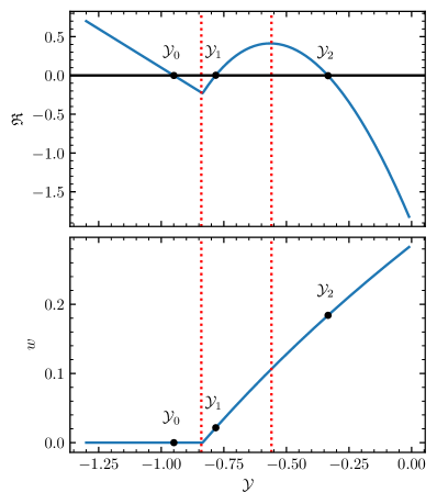
Figure 1: The residual of the luminosity equation $\mathfrak{R}$ (upper) and $w$ at the end of the time step (lower), plotted as functions of $\mathcal{Y}$ in a case where the correct $\mathcal{Y}<0$ and the initial $w>0$. Vertical dashed red lines denote the two special points $\mathcal{Y}_{0}$ (left) and $\mathcal{Y}_{1}$ (right). Input parameters were chosen so that there are three solutions to $\mathfrak{R}(\mathcal{Y})=0$ (black dots), with $L_{\rm solver}=0.1$, $L_{0}=2$, $\nabla_{\rm ad}=1$, $c_{0}=20$, $\xi_{1}=0$, $\xi_{2}=-1$, $w_{\rm initial}=1$, $|J|=\sqrt{-\mathcal{Y}}$, and $\delta t=t-t_{0}=5$, all in arbitrary units.

However, we do not know a priori how many solutions there are. There can be no more than three, but by changing $L_{\rm solver}$ we can make the example shown in Figure 1 have just one (convective) solution. Our approach is to first detect the number of solutions and isolate the one of physical interest.

The three solutions must be separated by two special points. The first ($\mathcal{Y}_{0}$) is the smallest-magnitude $\mathcal{Y}$ with $w=0$, and the second ($\mathcal{Y}_{1}$) is the $\mathcal{Y}$ such that $w>0$ and $\mathrm{d}\mathfrak{R}/\mathrm{d}\mathcal{Y}=0$. These are highlighted in Figure 1. Solutions of the first kind must occur at $\mathcal{Y}<\mathcal{Y}_{0}$, solutions of the second kind must occur at $\mathcal{Y}>\mathcal{Y}_{0}$, and at most one solution of the second kind occurs on either side of $\mathcal{Y}_{1}$.

Because ${\mathrm{d}w/\mathrm{d}\mathcal{Y}>0}$, we search for $\mathcal{Y}_{0}$ using bisection in the interval ${-100\leq\mathcal{Z}\leq 100}$. We likewise identify $\mathcal{Y}_{1}$ by a bisection search over $-100\leq\mathcal{Z}\leq\ln|\mathcal{Y}_{0}|$.

We use $\mathcal{Y}_{0}$ and $\mathcal{Y}_{1}$ to divide the interval ${-100\leq\mathcal{Z}\leq 100}$. The discriminant $\mathfrak{R}$ is monotonic over each subinterval by construction, so in each case we can search for a root using a combination of bisection search and Newton-Raphson refinement. We check the intervals in order, from nearest to $\mathcal{Y}=0$ to furthest, and terminate the search as soon as a root is found.

3.4.3 Relation to auto_diff

TDC returns $\mathcal{Y}$ given $L$ and the other solver variables. It additionally returns the partial derivatives of $\mathcal{Y}$ with respect to each of those variables. This relies, fundamentally, on the new automatic differentiation feature (see §2). In particular, we used auto_diff to calculate and propagate partial derivatives with respect to 33 variables of stellar structure through a Newton-Raphson solver, producing the partial derivatives of a root-finding procedure with respect to its inputs. The auto_diff functionality enables the implementation of TDC.

3.5 Reduction to Cox MLT

We now derive the modifications needed to ensure that TDC in MESA agrees with MLT in the limit of long time steps. While we use the $\alpha_{r}$ = 0 approximation in this section for clarity, the need for the correction is not removed by setting $\alpha_{r}>0$.

In TDC, the convective luminosity is given by Equation (7). In MLT, the convective luminosity is

$$L_{\rm conv}=4\pi r^{2}f_{2}\rho c_{P}Tv_{c}\Lambda(\nabla-\nabla_{e})h^{-1}$$ (18)

(Ludwig et al., 1999), where $v_{c}$ is the convective velocity and $f_{2}$ is a parameter dependent on the choice of MLT prescription. Finally, $\nabla_{e}$ is the temperature gradient of a convective eddy, which is related to the efficiency parameter

$$\Gamma\equiv\frac{\nabla-\nabla_{e}}{\nabla_{e}-\nabla_{\rm L}}.$$ (19)

We may write

$$\nabla-\nabla_{e}=\frac{\Gamma}{1+\Gamma}(\nabla-\nabla_{\rm L})=\frac{\Gamma}{1+\Gamma}\mathcal{Y},$$ (20)

so

$$L_{\rm conv}=\frac{\Gamma}{1+\Gamma}4\pi r^{2}f_{2}\rho c_{P}Tv_{c}\Lambda\mathcal{Y}h^{-1}.$$ (21)

Next we identify $w=\sqrt{3/2}v_{c}$ (in steady state) and $\Lambda=\alpha h$, so

$$L_{\rm conv}=4\pi r^{2}\alpha\frac{\Gamma}{1+\Gamma}\left(\frac{2}{3}f_{2}^{2}\right)^{1/2}\rho c_{P}Tw\mathcal{Y}.$$ (22)

This is nearly the same as Equation (7). In particular, in Cox MLT (Cox & Giuli, 1968) $f_{2}=1/2$ and

$$L_{\rm conv}=4\pi r^{2}\alpha\frac{\Gamma}{1+\Gamma}\rho c_{P}T\frac{w}{\sqrt{6}}\mathcal{Y},$$ (23)

so the only difference is the term involving $\Gamma$.

That term, which controls the convective efficiency, is a genuine difference between TDC-in-RSP and MLT. We want TDC in MESA to match the outputs of MLT in the steady state limit, in agreement with Kuhfuß (1986), we modify Equation (7) to include the factor $\Gamma/(1+\Gamma)$, giving

$$L_{\rm conv}=4\pi r^{2}\alpha\frac{\Gamma}{1+\Gamma}\rho c_{P}T\frac{w}{\sqrt{6}}\mathcal{Y}.$$ (24)

We evaluate $\Gamma$ by calling MLT with the same inputs as TDC. We then treat this as fixed during the TDC iterations, which allows us to still use the algorithm described in §3.4.

With these modifications, the luminosity equations now agree, subject to $w=\sqrt{3/2}v_{c}$ in steady state. We now derive the conditions required to make this hold.

In MLT, the convective velocity is given by

$$v_{c}^{2}=f_{1}\Lambda^{2}g\delta(\nabla-\nabla_{e})h^{-1},$$ (25)

where $f_{1}$ is a parameter determined by the choice of MLT and

$$\delta\equiv-\left.\frac{\partial\ln\rho}{\partial\ln T}\right|_{P}=\frac{\chi_{T}}{\chi_{\rho}}.$$ (26)

Using $\Lambda\equiv\alpha h$ we can write Equation (25) as

$$v_{c}^{2}=\alpha^{2}f_{1}hg\frac{\chi_{T}}{\chi_{\rho}}(\nabla-\nabla_{e}).$$ (27)

Next, with Equation (20) we find

$$v_{c}^{2}=\alpha^{2}f_{1}hg\frac{\chi_{T}}{\chi_{\rho}}\frac{\Gamma}{1+\Gamma}\mathcal{Y}.$$ (28)

In TDC, we have identified the convection speed with $v_{c}\equiv\sqrt{2/3}w$, so we now proceed to prove that this is equivalent to that given by Equation (28). When the TDC discriminant $J^{2}<0$, then $\mathcal{Y}<0$ so the system is subadiabatic. Hence, at long times $w=0$ and therefore $v_{c}=0$, which matches the MLT answer. When the discriminant is positive the system is convectively unstable, so we use Equation (12) and find

$$v_{c}=-\sqrt{\frac{2}{3}}\frac{1}{2\xi_{2}}\left(J\tanh\frac{\lambda+\delta tJ}{4}+\xi_{1}\right).$$ (29)

This solution was constructed assuming not only that $J^{2}>0$ but also that the relevant root is $J>0$. As $\delta t\rightarrow\infty$ the $\tanh$ term approaches unity. In this limit

$$v_{c}=-\sqrt{\frac{1}{6}}\frac{1}{\xi_{2}}\left(J+\xi_{1}\right)~{},$$ (30)

and we also have $\xi_{1}=0$ because $\mathrm{D}\rho/\mathrm{D}t=0$ and $\alpha_{r}=0$ (Equation 10). Inserting the definition of $J$ and expanding with Equations (9) and (11) we find

$$v_{c}^{2}=\frac{1}{6}\frac{J^{2}}{\xi_{2}^{2}}=-\frac{2\xi_{0}}{3\xi_{2}}=\frac{\alpha^{2}c_{P}T\nabla_{\rm ad}\mathcal{Y}}{8\alpha_{D}}~{}.$$ (31)

Comparing this with Equation (28), for equality

$$\frac{\alpha^{2}c_{P}T\nabla_{\rm ad}\mathcal{Y}_{\rm MLT}}{8\alpha_{D}}=\alpha^{2}f_{1}hg\frac{\chi_{T}}{\chi_{\rho}}\frac{\Gamma}{1+\Gamma}\mathcal{Y}_{\rm TDC}.$$ (32)

As before, to obtain equivalence between MLT and TDC we need to substitute $\mathcal{Y}\Gamma/(1+\Gamma)$ for $\mathcal{Y}$ in the velocity equation. In addition, we need to have

$$\frac{c_{P}T\nabla_{\rm ad}}{8\alpha_{D}}=f_{1}hg\frac{\chi_{T}}{\chi_{\rho}}.$$ (33)

With some rearranging, and using $h=P/\rho g$, we find

$$\frac{1}{8\alpha_{D}f_{1}}=\frac{P\chi_{T}}{\chi_{\rho}\rho c_{P}T\nabla_{\rm ad}}.$$ (34)

With $\Gamma_{3}=1+(P/\rho c_{V}T)\chi_{T}$,

$$\frac{1}{8\alpha_{D}f_{1}}=(\Gamma_{3}-1)\frac{c_{V}}{\chi_{\rho}c_{P}\nabla_{\rm ad}}=\frac{\Gamma_{3}-1}{\Gamma_{1}\nabla_{\rm ad}}=1.$$ (35)

In Cox MLT $f_{1}=1/8$, and in TDC by default $\alpha_{D}=1$, so the two sides are equal.

The net result is that in the limit of long time steps, TDC and Cox MLT solve the same luminosity equation with the same inputs and so are mathematically identical. We find they agree numerically to around seven decimal places in $\mathcal{Y}$, even when $\mathcal{Y}\ll 1$. The need for the correction is not removed by setting $\alpha_{r}>0$. The asymptotic scaling in the inefficient limit is qualitatively different between (TDC with no correction and $\alpha_{r}>0$) and (TDC with correction and $\alpha_{r}$ = 0). We further implement the calculation of convective mixing diffusivity and all other derived quantities using $v_{c}$ in the same way in both TDC and Cox MLT.

Figure 2 shows the importance of the $\mathcal{Y}\rightarrow\mathcal{Y}\Gamma/(1+\Gamma)$ correction. In both panels, the solutions for TDC and MLT lie on top of each other. The solution for TDC without the correction of $\mathcal{Y}$ in the equations, by contrast, deviates significantly in both panels. This deviation is starkest in the lower panel, which shows a different $v_{c}$ scaling in the inefficient ($\nabla_{\rm rad}-\nabla_{\rm ad}\ll 1$) limit.

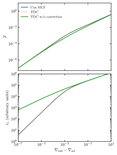
Figure 2: The values of $\mathcal{Y}$ (upper) and $v_{c}$ (lower) plotted as functions of $\nabla_{\rm rad}-\nabla_{\rm ad}$ for MLT, TDC, and TDC without the correction $\mathcal{Y}\rightarrow\mathcal{Y}\Gamma/(1+\Gamma)$ in the convective velocity and luminosity equations. The time step was chosen to be long enough that TDC reaches equilibrium.

3.6 Accreting White Dwarfs

WDs accreting He at rates $\lesssim 10^{-6}\,\mathrm{M}_{\odot}\,{\mathrm{yr}}^{-1}$ undergo He shell flashes (Iben & Tutukov, 1989). These flashes can lead to He nova (e.g., V445 Puppis; Ashok & Banerjee, 2003), or even double-detonation type Ia supernovae (e.g., Shen & Bildsten, 2009; Woosley & Kasen, 2011; Kupfer et al., 2022). The time-dependent burning is controlled by three timescales: the local nuclear heating time,

$$t_{\rm heat}\equiv\frac{c_{P}T}{\epsilon_{\mathrm{nuc}}},$$ (36)

being the characteristic timescale for temperature changes due to nuclear burning; the convective acceleration time,

$$t_{\rm accel}\equiv\frac{4}{J}=\frac{3h}{\sqrt{2\alpha_{D}c_{P}T\nabla_{{\rm ad}}\mathcal{Y}}},$$ (37)

being the timescale over which convection varies (see Equation 12); and the local dynamical time,

$$t_{\rm dyn}\equiv\frac{h}{c_{\rm s}}.$$ (38)

In steady state $t_{\rm accel}$ is proportional to the eddy turnover time

$$t_{\rm eddy}\equiv\frac{\alpha h}{v_{c}},$$ (39)

but in cases of interest $t_{\rm accel}$ and $t_{\rm eddy}$ can be quite different.

Shen & Bildsten (2009) showed that He shell masses of $\gtrsim 0.03\,\mathrm{M}_{\odot}$ on a $\approx 1\,\mathrm{M}_{\odot}$ WD can yield a $t_{\rm heat}$ comparable to or shorter than $t_{\rm accel}$ or even $t_{\rm dyn}$ near the base of the convection zone (BCZ). TDC will yield different results than MLT in this limit.

We construct these He flash models by accreting material comprising 99% ${}^{4}{\rm He}$ and 1% ${}^{14}{\rm N}$ by mass (as expected for solar metallicity stars that have undergone CNO burning) onto a $1\,\mathrm{M}_{\odot}$ carbon-oxygen WD at constant $\log(\dot{M}/\mathrm{M}_{\odot}\,{\mathrm{yr}}^{-1})$ between $-7.1$ and $-7.4$ in steps of $0.1$ dex. Compressional heating results in a local temperature increase until the He shell ignites. Lower $\dot{M}$ results in weaker compressional heating and a more massive He shell at ignition. Because heat is transported from the temperature peak towards both the core and the surface, ignition occurs above the base of the freshly accreted layer. We stop the accretion once a convective zone appears at the ignition site, and continue evolving through the He flash. Both the total accumulated He shell mass and location of ignition are impacted by the included reaction chain ${}^{14}{\rm N}(e^{-},\nu){{}^{14}{\rm C}}(\alpha,\gamma){{}^{18}{\rm O}}$ (NCO, Hashimoto et al. 1986; Bauer et al. 2017).

In Figure 3, we label our models 1–4 at different $\dot{M}$ (with 1 corresponding to $-7.1$, 2 to $-7.2$, etc.) and note the masses enclosed by and exterior to the base of the convection zone (BCZ), which set the pressure $P_{\rm BCZ}$ at ignition. The total accumulated He shell mass ranges from $0.03$ to $0.08\,\mathrm{M}_{\odot}$.

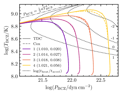
Figure 3: Evolution of $T_{\rm BCZ}$ and $P_{\rm BCZ}$ during a He flash on a $1\,\mathrm{M}_{\odot}$ WD with various He shell masses. Solid and dashed lines correspond to models run with TDC and Cox MLT respectively. The values in parentheses indicate the masses in solar units enclosed within and exterior to the BCZ, respectively. Dotted lines are contours of fixed logarithmic ratio between $t_{\rm heat}$ and $t_{\rm accel}$, from $-2$ to $1$. Dot-dashed line gives the radiation pressure.

Figure 3 shows the evolution of $T_{\rm BCZ}$ and $P_{\rm BCZ}$ for models 1–4 with both TDC and Cox MLT. All models initially evolve at nearly constant $P_{\rm BCZ}$, which increases with He shell mass. As temperature increases in the convection zone, the envelope expands and reduces $P_{\rm BCZ}$. Concurrently, $T_{\rm BCZ}$ reaches a maximum (Shen & Bildsten, 2009). Thicker He shells reach higher peak $T_{\rm BCZ}$ and larger ratios between $t_{\rm heat}$ and $t_{\rm accel}$. For the contours here, $t_{\rm accel}\approx 10\,t_{\rm dyn}$ (e.g., model 4 reaches $t_{\rm heat}/t_{\rm accel}\approx 0.01$, and correspondingly $t_{\rm heat}/t_{\rm dyn}\approx 0.1$.) When models show $t_{\rm heat}\lesssim t_{\rm accel}$ (models 3 & 4) and start expanding, TDC starts to deviate from Cox MLT, with greater deviations for thicker He shells. TDC shows higher $T_{\rm BCZ}$ than Cox MLT at fixed $P_{\rm BCZ}$ because TDC results in more superadiabatic convection. In contrast, when $t_{\rm heat}\gtrsim t_{\rm accel}$ (models 1 & 2) TDC and Cox MLT show good agreement in the evolution of $P_{\rm BCZ}$ and $T_{\rm BCZ}$.

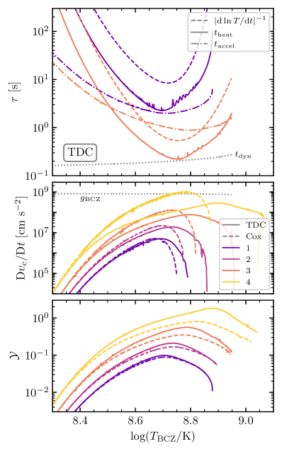
Figure 4: Evolution of various time scales in the convection zone (upper), the time derivative of convective velocity at a fixed mass coordinate (middle), and the superadiabaticity at the same location (lower). The upper panel compares the heating timescale (solid line), actual timescale for temperature change (dashed line), convective acceleration timescale (dot-dashed line), and dynamical timescale (dotted line), for models 1 and 3 (TDC only). The first three timescales are evaluated at the BCZ, and the last at maximum convective velocity. Line styles in the middle and lower panels follow that of Figure 3, and in the middle panel we show the gravitational acceleration at the BCZ ($g_{\rm BCZ}$, dotted line) for comparison.

The upper panel of Figure 4 compares several timescales for TDC models 1 & 3. The heating timescale, $t_{\rm heat}$, trends similarly with $\left|\mathrm{d}\ln T/\mathrm{d}t\right|^{-1}$, but the latter is larger than $t_{\rm heat}$ by factors of a few, because heat released by nuclear burning is distributed throughout some portion of the convection zone. Due to the sharp dependence of $\epsilon_{\mathrm{nuc}}$ on $T$, both timescales decrease sharply with $T_{\rm BCZ}$ until the WD starts to expand. To reduce the noise in $\left|\mathrm{d}\ln T/\mathrm{d}t\right|^{-1}$ displayed in Figure 4, we fit it with a polylogarithmic function. The difference between $t_{\rm heat}$ and $\left|\mathrm{d}\ln T/\mathrm{d}t\right|^{-1}$ decreases with thicker He shells, as heat released by nuclear burning is increasingly trapped locally.

Another relevant timescale is $t_{\rm accel}$, evaluated at maximum $v_{c}$. At $\log(T_{\rm BCZ}/\mathrm{K})\lesssim 8.4$, $t_{\rm accel}\approx(3/4)t_{\rm eddy}$. At $\log(T_{\rm BCZ}/\mathrm{K})\gtrsim 8.4$, $t_{\rm accel}$ evolves more quickly than $t_{\rm eddy}$, becoming up to 3 (6) times smaller than $t_{\rm eddy}$ in model 3 (4). This is because convection is no longer in steady-state, as $t_{\rm heat}\lesssim t_{\rm accel}$ for $\log(T_{\rm BCZ}/\mathrm{K})\gtrsim 8.4-8.5$ (see also Glasner et al., 2018). At minimum $t_{\rm heat}$, the hierarchy of timescales changes from — $\mathrm{d}$lnT / $\mathrm{d}$t —^-1≳t_heat≳t_accel≫t_dyn to t_accel≳— $\mathrm{d}$lnT / $\mathrm{d}$t —^-1≳t_heat≳t_dyn from model 1 to model 3, and ultimately to t_accel≳t_dyn≳— $\mathrm{d}$lnT / $\mathrm{d}$t —^-1≳t_heat in model 4. The fact that convection is not able to reach a steady state on the evolutionary timescale of the He flash explains the difference between TDC and Cox MLT in models 3 & 4 (see Figure 3).

We illustrate the difference in the evolution of $v_{c}$ and $\mathcal{Y}$ between TDC and Cox MLT in the middle and lower panels of Figure 4. For each TDC and Cox MLT pair, we locate the mass coordinate at which $v_{c}$ peaks when $\log(L_{\mathrm{nuc}}/\mathrm{L}_{\odot})=9$ (arbitrarily chosen), and evaluate $\mathrm{D}v_{c}/\mathrm{D}t$ and $\mathcal{Y}$ during the initial acceleration phase. Initially, TDC and Cox MLT show good agreement when $t_{\mathrm{heat}}\gg t_{\mathrm{accel}}$ ($\log(T_{\mathrm{bcz}}/\mathrm{K})\lesssim 8.4$). When $t_{\mathrm{heat}}\lesssim t_{\mathrm{accel}}$ ($\log(T_{\mathrm{bcz}}/\mathrm{K})\gtrsim 8.5$), TDC shows slower evolution in $v_{c}$ and larger $\mathcal{Y}$ than Cox MLT. As $v_{c}$ is lower in TDC, heat is less efficiently transported out of the BCZ, resulting in higher $T_{\rm BCZ}$ and $\mathcal{Y}$ near maximum. With a thicker He shell, $\mathrm{D}v_{c}/\mathrm{D}t$ may become comparable to $g$ (especially for Cox MLT model 4).

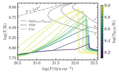
Figure 5: Profiles of $T$ and $P$ within model 3 at different moments, when both TDC (solid) and Cox MLT (dashed) reach the same $T_{\rm BCZ}$. Curves of same color correspond to identical $T_{\rm BCZ}$. Dotted and dot-dashed lines take the same meaning as in Figure 3.

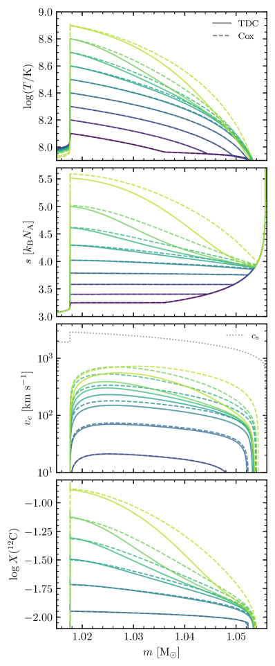
Figure 6: Same as Figure 5, but instead showing $T$, $s$, $v_{c}$, and $X(^{12}{\rm C})$ as a function of mass coordinate from top to bottom. In the third panel, $c_{\rm s}$ is shown for comparison. The colors match the colorbar in Figure 5.

We now study the evolution of model 3 in detail. In Figure 5, we compare seven snapshots of the TDC and Cox MLT models in $T-P$ space, when both reach the same $T_{\rm BCZ}$. The three coolest pairs of curves show good agreement and little superadiabaticity (third panel of Figure 4). For the subsequent three hotter pairs, $\mathcal{Y}$ grows up to order unity near peak $T_{\rm BCZ}$. Once $t_{\mathrm{heat}}\lesssim t_{\mathrm{accel}}$, heat is trapped more locally in TDC compared to Cox MLT. Therefore, TDC reaches the same $T_{\rm BCZ}$ earlier in the evolution, and has a higher $P_{\rm BCZ}$ due to comparably colder outer layers. Likewise, TDC shows less evolution in $T-P$ near the top of the convection zone and more superadiabaticity near the BCZ, again because of stronger heat-trapping near the BCZ.

Figure 6 compares TDC and Cox MLT in model 3 as a function of mass coordinate. The two show reasonable agreement in $v_{c}$ when $\log(T_{\rm BCZ}/\mathrm{K})\lesssim 8.5$. At this point, $t_{\rm heat}$ drops below $t_{\rm accel}$ (see Figure 4), which leads to TDC yielding lower $v_{c}$ than Cox MLT. For the same reason, $v_{c}$ near the top of the convection zone appears frozen in TDC for $8.6\lesssim\log(T_{\rm BCZ}/\mathrm{K})\lesssim 8.8$.

At fixed $T_{\rm BCZ}$, TDC shows lower $T$ throughout the convection zone, reflecting a local buildup of heat at the BCZ. Since TDC carries heat out of the BCZ less efficiently, it also shows a stronger entropy gradient, and for ${8.6\lesssim\log(T_{\rm BCZ}/\mathrm{K})\lesssim 8.8}$, $T$ and $s$ show little evolution near the top of the convection zone.

Both TDC and Cox MLT show appreciable abundance gradients, as $\mathrm{{}^{12}C}$ is produced near the BCZ but there is insufficient time for it to be transported outwards. Cox MLT shows higher $\mathrm{{}^{12}C}$ abundance overall, as it has more time to reach the same $T_{\rm BCZ}$ and larger $v_{c}$. As TDC modifies both the $T$ and $X_{i}$ profiles, it may impact the potential for the ignition to develop into a detonation that would result in a thermonuclear transient.

In summary, we see that convection in TDC adjusts more slowly to changes in heating than in Cox MLT. This results in slower, more superadiabatic convection during rapidly-burning phases of evolution. The incorporation of the dynamics of how convection grows and decays is now possible and enabled by default in MESA via TDC.

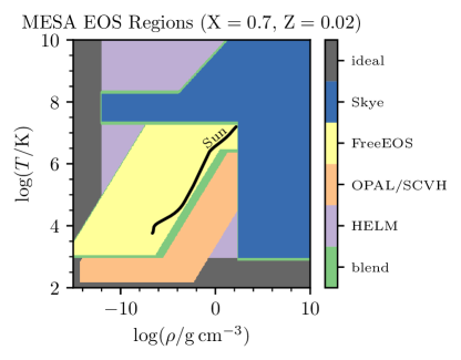
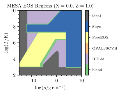
Figure 7: Default EOS boundaries for a solar-like composition (Z = 0.02, left) and for a pure-metal composition (Z = 1, 50% ¹²C and 50% ¹⁶O by mass, right). The colors and labels indicate an ideal gas approximation, Skye, FreeEOS, OPAL, SCVH, HELM, and blends between two EOSs. The black curve in the left panel shows a model for the present day Sun.

4 Equation of State

MESA models require thermodynamic quantities over a large span of $T$, $\rho$, and $X_{i}$. This involves calling the MESA EOS $\sim 10^{4}$–$10^{10}$ times, depending on the chosen local physics and the number of iterations, cells, and time steps. It would be ideal to have a single EOS that accurately represents the relevant physics in all regimes, obeys all thermodynamic consistency relations to the limits of the arithmetic, and is as efficient in storage and execution as possible. Below we report progress towards this ideal.

Figure 7 shows the default MESA EOS boundaries for solar and pure-metal (50% ¹²C, 50% ¹⁶O by mass) compositions. Broadly, we prioritize HELM (Timmes & Swesty, 2000) at high $T$ and low $\rho$ for handling of the electron-positron plasma. Elsewhere we prioritize Skye (Jermyn et al., 2021), limited by partial ionization at lower $T$ and $\rho$. We then prioritize FreeEOS (Irwin, 2004), then OPAL (Rogers & Nayfonov, 2002) and SCVH (Saumon et al., 1995), and finally, when there are no other options, we use an ideal gas with radiation. Blending boundaries between the different EOS prescriptions are set to defaults that have been motivated by specific use cases. For example, we have chosen the boundaries between FreeEOS and Skye such that solar models at the age of the Sun stay fully on FreeEOS and do not encounter the FreeEOS-Skye blend.

4.1 Skye

Skye is an EOS for fully ionized matter (Jermyn et al., 2021). A motivation for developing Skye was eliminating the blend between HELM and PC (Potekhin & Chabrier, 2010). There is a blend between HELM and Skye that occurs at much higher $T$ and lower $\rho$ (see Figure 7), where the two agree. Skye includes the effects of positrons, relativity, and electron degeneracy (Timmes & Swesty, 2000; Baturin et al., 2019), Coulomb interactions (Ichimaru et al., 1987; Potekhin & Chabrier, 2010, 2000; DeWitt & Slattery, 1999; Baiko et al., 2001; Farouki & Hamaguchi, 1993), non-linear mixing effects (Caillol, 1999; Potekhin et al., 2009; Potekhin & Chabrier, 2013; Ogata et al., 1993; Medin & Cumming, 2010), and quantum corrections (Hansen & Vieillefosse, 1975; Nagara et al., 1987; Carr et al., 1961; Potekhin & Chabrier, 2000, 2010; Baiko, 2019; Baiko & Chugunov, 2022). Skye determines the point of Coulomb crystallization in a self-consistent manner, accounting for mixing and composition effects. A defining feature of Skye is the use of analytic Helmholtz free energy terms and automatic differentiation (see §2) to provide thermodynamic quantities. Skye is thus readily extendable to new physics by including additional terms in the free energy (Jermyn & Timmes, 2022).

Skye is both a standalone software instrument and integrated into MESA. The two implement the same input physics and options. At times this has required modifications of other parts of MESA. Here we describe the most important of these modifications.

4.1.1 Crystallization

Skye determines the crystallization phase transition by minimizing the Helmholtz free energy, which permits derivatives to be discontinuous at the transition. For instance, the entropy discontinuity reflects the latent heat of crystallization. This posed a challenge in MESA. Consider the expression

$$\epsilon_{\rm grav}\equiv-T\frac{\mathrm{D}s}{\mathrm{D}t}~{}.$$ (40)

The entropy $s\equiv-\partial F/\partial T|_{\rho}$ undergoes a discontinuity at the phase transition. If D$s$/D$t$ is evaluated by finite differences, then no time step will be small enough to produce a converged result for $\epsilon_{\rm grav}$. We could write

$$\frac{\mathrm{D}s}{\mathrm{D}t}=\left.\frac{\partial s}{\partial T}\right|_{\rho}\frac{\mathrm{D}T}{\mathrm{D}t}+\left.\frac{\partial s}{\partial\rho}\right|_{T}\frac{\mathrm{D}\rho}{\mathrm{D}t},$$ (41)

but this form misses the latent heat of the phase transition because, except for the infinitesimal vicinity of crystallization, thermodynamic derivatives of $s$ contain no information about the transition. At the phase transition, derivatives of $s$ contain a Dirac delta contribution, which cannot be directly implemented in numerical calculations. The choice is between poor convergence (finite differences of $s$) or neglecting the latent heat (Equation 41).

To address crystallization, Skye returns a parameter $\phi$ that provides a smoothed representation of the phase. Specifically, $\phi=1$ in the solid phase, $\phi=0$ in the liquid phase, and near the phase transition $\phi$ smoothly interpolates between these limits. The transition in $\phi$ is tuned so that the crystallization boundary is numerically resolved and yet spans a small fraction of a stellar model. Using $\phi$, Skye then constructs a smoothed version of the latent heat of crystallization, which is only significant in the transition region. This allows use of Equation (41) to avoid numerical issues near the phase transition, but requires that we include an extra heat source in the energy equation to capture the latent heat:

$$\epsilon_{\rm latent}\equiv L_{T}\frac{\mathrm{D}\ln T}{\mathrm{D}t}+L_{\rho}\frac{\mathrm{D}\ln\rho}{\mathrm{D}t},$$ (42)

where $L_{T}$ and $L_{\rho}$ represent the differences between smoothed and original versions of the entropy derivatives $T\partial s/\partial\ln T$ and $T\partial s/\partial\ln\rho$. The original derivatives lack the latent heat, while the smoothed ones contain it, so $L_{T}$ and $L_{\rho}$ produce additional heating. With this procedure, MESA is able to model phase transitions, remain numerically converged, and accurately capture the latent heat of crystallization. This procedure smears only the latent heat of crystallization and does not smear the thermodynamics of the phase transition, which would produce unphysical results such as negative sound speeds.

The Skye EOS approach represents a significant improvement for the MESA latent heat treatment. Previously, MESA relied on a finite difference of the entropy calculated in the PC EOS for solid and liquid phases so that latent heat could be included in $\epsilon_{\mathrm{grav}}$via Equation (40), smoothing this quantity near the phase transition for numerical convergence (MESA IV). Another common approach is to include latent heat release with an explicit heating term using $l_{\rm cr}\approx 0.77k_{\rm B}T/\langle A\rangle m_{\rm p}$ based on the calculation of Salaris et al. (2000). Our new approach based on Skye has the advantage that the phase diagram and latent heat release are both calculated from first principles and are self-consistent with the underlying thermodynamics of the EOS. Jermyn et al. (2021) showed that the net latent heat release is commensurate with the Salaris et al. (2000) value.

4.2 FreeEOS

We use FreeEOS version 2.2.1 (Irwin, 2004) to expand the chemical composition parameter space covered by partial ionization, as compared to the OPAL tables. This replaces the eosPTEH tables of MESA V. FreeEOS minimizes a Helmholtz free energy to span essentially the same thermodynamic range as OPAL.

The FreeEOS tables generated for MESA use the ‘EOS1’ mode, which is the highest level of physical accuracy provided by FreeEOS. The tables are parameterized by the metal mass fraction $\rm{Z}=0$, 0.02, 0.04, 0.06, 0.08, 0.10, 0.20, 0.30, 0.40, 0.50, 0.60, 0.70, 0.80, 0.90, and 1.00. All tables assumed a scaled-solar chemical composition based on Grevesse & Sauval (1998). For Z $\geq$ 0.80, there is also a set of tables with $X(^{12}$C) = $X(^{16}$O) for use with WD interiors. For each Z a range of H mass fraction values between 0 and $1-\rm{Z}$ are provided, allowing for a complementary range of He mass fractions. The tools to generate a new set of MESA EOS tables for an arbitrary chemical composition using FreeEOS are provided in MESA_DIR/eos/eosFreeEOS_builder with the exception of the FreeEOS library, which can be downloaded from the FreeEOS repository.

4.3 EOS Blends

The MESA EOS blends several EOS prescriptions. Each EOS returns fundamental quantities and the partial derivatives of those quantities. The blends of fundamental quantities and derivatives are treated differently because they are used by MESA for different purposes. Fundamental quantities enter into physical equations, and so must be physical (e.g., positive sound speed), while their derivatives are used to construct the solver Jacobian, and so must represent accurate derivatives of the fundamental quantities.

The EOS returns a vector res containing fundamental EOS quantities such as $e$, $s$, and $c_{V}$ (see MESA I Table 3), as well as blending fractions for the various EOS components. The EOS also returns corresponding vectors d_dlnd and d_dlnT of partial derivatives of each of the quantities in res with respect to $\rho$ and $T$.

At the boundary between a pair of EOS prescriptions (EOS1 and EOS2) we calculate blends of res, d_dlnd and d_dlnT independently. The EOS at a point in the blending region between EOS1 and EOS2 is evaluated with blending coefficient $\alpha\in[0,1]$ representing the fraction of EOS1, and $1-\alpha$ representing the fraction of EOS2. We construct blending coefficients using the quintic polynomial

$$\alpha=6x^{5}-15x^{4}+10x^{3}~{},$$ (43)

which maps the interval $x\in[0,1]$ (representing distance across a blend in $\rho$ or $T$) onto the interval $\alpha\in[0,1]$ with zero slope at the blending boundaries. The blending coefficients therefore have non-zero derivatives with respect to $\rho$ and $T$ in blending regions. Quantities in the resulting $\texttt{res}_{\rm blend}$ vector are evaluated as a linear mix using the blending coefficient,

$$\texttt{res}_{\rm blend}=\alpha\,\texttt{res}_{1}+(1-\alpha)\,\texttt{res}_{2}~{}.$$ (44)

Our choice of a quintic polynomial for the blending coefficient ensures that both $\alpha$ and $(1-\alpha)$ are non-negative everywhere in the blending region, and therefore the EOS blending never introduces negative quantities into blends of non-negative values for the EOS res vector. For the derivative vectors, we include additional terms to account for the derivatives of the blending coefficients,

$$\begin{split}\texttt{d\_dlnd}_{\rm blend}=&\alpha\,\texttt{d\_dlnd}_{1}+\frac{\partial\alpha}{\partial\ln\rho}\texttt{res}_{1}\\ &+(1-\alpha)\,\texttt{d\_dlnd}_{2}-\frac{\partial\alpha}{\partial\ln\rho}\texttt{res}_{2}~{},\end{split}$$ (45)

and similarly for d_dlnT. Including these terms for the blending coefficients in the derivative blends provides correct derivatives for the solver, reducing the number of Newton iterations.

Some quantities in the fundamental EOS res vector are themselves derivatives of other EOS quantities, such as $c_{V}\equiv(\partial e/\partial T)_{\rho}$. The different blending treatments for EOS quantities and their derivatives mean that thermodynamic identities may be violated in blending regions. Physical equations such as the energy equation must use quantities such as $c_{V}$ from res rather than the theoretically equivalent but numerically different derivative quantities from the d_dlnT vector. The latter can lead to unphysical results such as negative heat capacities or negative sound speeds. This inconsistency is unavoidable so long as we must blend between different EOS prescriptions.

4.4 Thermodynamic Consistency

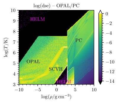
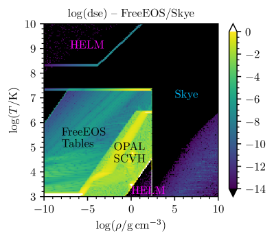
Figure 8: The logarithm of the thermodynamic consistency measure $\mathrm{dse}$ for the MESA EOS computed with PC and OPAL (left) and Skye and FreeEOS (right) with $\rm{X}=0.7$, $\rm{Y}=0.28$, and $\rm{Z}=0.02$, with $\rm{Z}$ comprising equal mass fractions of ${}^{12}\mathrm{C}$ and ${}^{16}\mathrm{O}$.

One desirable feature in an EOS is thermodynamic consistency, which ensures that the Maxwell relations hold — e.g., mathematically equivalent forms of the equations of stellar structure are also numerically equivalent within the floating point precision of the arithmetic. Unfortunately, several of the EOS prescriptions in MESA are not fully thermodynamically consistent. This can cause errors in energy conservation, making mathematically equivalent formulations of the structure equations behave differently.

Here we report on the current state of thermodynamic consistency in MESA. Figure 8 compares the consistency measure

$$\mathrm{dse}\equiv T\frac{\partial s/\partial T|_{\rho}}{\partial e/\partial T|_{\rho}}-1$$ (46)

for the MESA EOS with PC and OPAL (left, former default) and with Skye and FreeEOS (right, current default). The quantity $\mathrm{dse}$ is zero in thermodynamically consistent systems.

As Skye derives all quantities from partial derivatives of a Helmholtz free energy, it is thermodynamically consistent to near machine precision. Without Skye, the corresponding regions of the EOS are covered by PC and HELM. The regions with Skye active show thermodynamic consistency to near machine precision, representing a significant improvement for $\log(\rho/\mathrm{g\,cm^{-3}})\gtrsim 3$. The band at $\log\left(T/\mathrm{K}\right)\approx 9-10$ in the right panel is due to a blend in the EOS from Skye to HELM, which is required to remedy a floating point loss-of-precision issue in Skye when electron-positron pairs dominate the EOS. In the left panel the PC region shows a stripe of high error due to Coulomb crystallization. FreeEOS is thermodynamically consistent to near machine precision. Our current method of interpolating the MESA FreeEOS tables does not preserve this property. Still, these tables show significant improvement relative to OPAL.

5 Energy Equations

Section 3 of MESA V highlighted the importance of numerical energy conservation in MESA models, and introduced a new form of the energy equation aimed at improving energy conservation. This new form motivated several solver improvements, leading to tighter tolerances for equation residuals and corrections. We now advance that discussion by further explaining the multiple formulations of the energy equations in MESA. We contrast the advantages conferred by each formulation across different applications. We also clarify the meaning of the quantities rel_E_err and rel_run_E_err reported for MESA runs, and elucidate what these quantities do and do not tell us about the quality of the MESA solutions.

After reviewing the energy-equation fundamentals and recent implementation improvements in §5.1, we explore an idealized example problem without any composition changes or EOS complexities in §5.2. This example motivates a new time-centered approach for evaluating the eps_grav form of the energy equation, and demonstrates that a lower value of rel_run_E_err does not always indicate evolution that is more physically accurate. In §5.3 we describe the additional complexities introduced by thermodynamic inconsistencies that can be present in the EOS, especially in EOS blending regions, and how these manifest in different ways for different energy equation implementations.

Finally, in §5.4 we illustrate the various contributions to energy error terms through the example of a $1\,\mathrm{M}_{\odot}$ star including both composition changes due to nuclear burning and EOS blends and inconsistencies. This example demonstrates that the quantity rel_run_E_err must be interpreted differently for different forms of the energy equation. When using the dedt form of the energy equation, the energy error reflects the quality of the residuals from the MESA solver, even though larger energy errors associated with the EOS are still present in the model. When using the eps_grav form of the energy equation, the energy error reports much larger values that reflect the presence of these EOS errors, even when the quality of solutions may be comparable to or better than the dedt form.

Convergence tests and comparisons between multiple forms of the energy equation remain vital for understanding the reliability and accuracy of solutions in different regimes. Significant progress has been made in ensuring that different forms of the energy equation converge to the same result. In degenerate conditions, the eps_grav forms generally perform better (i.e., they are closer to the converged answer at a given time resolution). With the dedt form, the numerical energy conservation error often measures the quality of the solution (i.e., the size of the residuals). Focusing on improving that quantity has driven significant solver improvements and motivated the development of an accurate energy accounting infrastructure. This energy accounting work has also motivated improving the eps_grav form to account for composition changes, as well as an implicit trapezoidal time-centering scheme. MESA now includes these changes by default when using the eps_grav form of the energy equation. Further progress rests on improvements to the quality of the EOS.

5.1 Fundamentals and Implementations

MESA has two primary energy equations. One, called the “eps_grav form”, is the standard stellar structure energy equation (e.g., Kippenhahn et al., 2012) and is the equation introduced in MESA I. This equation is

$$\frac{\partial L}{\partial m}=\epsilon+\epsilon_{\mathrm{grav}}~{},$$ (47)

where $L$ is the luminosity, $\epsilon$ is a specific energy generation source term (e.g., nuclear reactions, neutrinos), and

$$\begin{split}\epsilon_{\mathrm{grav}}&\equiv-\frac{\mathrm{D}e}{\mathrm{D}t}+P\frac{\mathrm{D}}{\mathrm{D}t}\left(\frac{1}{\rho}\right)\\ &=-T\frac{\mathrm{D}s}{\mathrm{D}t}-\sum_{i}\left(\frac{\partial e}{\partial X_{i}}\right)_{s,\rho,\{X\neq X_{i}\}}\frac{\mathrm{D}X_{i}}{\mathrm{D}t}~{}.\end{split}$$ (48)

In practice, the total Lagrangian time derivative of $e$ is expanded and further manipulated to reach the final form evaluated in MESA (see MESA IV, §8).

The other, called the “dedt form”, is an energy equation for the time evolution of the total specific energy of a Lagrangian cell,

$$\frac{\mathrm{D}}{\mathrm{D}t}\left(e+\frac{1}{2}u^{2}-\frac{Gm}{r}\right)=\epsilon-\frac{\partial}{\partial m}\left(L+P\mathcal{A}\,u\right)~{},$$ (49)

where $u$ is cell velocity and $\mathcal{A}=4\pi r^{2}$ is the area of the cell face. The relationship between these two forms was derived in MESA IV, Section 8.3 and the dedt form was introduced as a powerful tool in support of improved numerical energy conservation in MESA V, §3.

When solutions are numerically converged (i.e., have sufficient space/time resolution to give resolution-independent results) and the EOS is thermodynamically consistent and provides correct partial derivatives (see §5.3), these two equations should give identical results. Conversely, the solutions may differ when unconverged.

The error in numerical energy conservation during a step, $E_{\rm err}^{\rm step}$, is evaluated as the difference between the change in total energy of the model across the time step and the expected change in total energy due to known energy sources and sinks (e.g., nuclear reactions, neutrinos, surface luminosity). Total energy is defined as

$$\begin{split}E_{\rm tot}&\equiv\int\left(e+\frac{1}{2}u^{2}-\frac{Gm}{r}\right)\,\mathrm{d}m\\ &=\sum_{k}dm_{k}\left(e_{k}+\frac{1}{2}u_{k}^{2}-\frac{Gm_{k}}{r_{k}}\right)~{},\end{split}$$ (50)

where $dm_{k}$ is the mass contained within cell $k$. Additional terms for rotational kinetic energy can also be included in Equation (50) when rotation is enabled, and turbulent energy is included for RSP models.

A cumulative sum of the per-step energy errors, $E_{\rm err}^{\rm run}$, is tracked during a run. When divided by the total energy at the end of the step, $E_{\rm err}^{\rm step}$ and $E_{\rm err}^{\rm run}$ respectively become the quantities rel_E_err and rel_run_E_err that are reported by MESA. As stated in MESA V, these quantities are primarily meant to represent a measure of the numerical reliability of solutions accepted for MESA evolution steps, rather than a measure of physical validity and completeness of MESA models. In §5.3 and §5.4, we focus on further clarifying the meaning of these energy error quantities, which require a different interpretation when using the eps_grav form of the energy equation than when using the dedt form.

MESA does not solve its discretized, finite-mass form of the stellar structure equations exactly. When a trial solution is accepted, the residual difference between the left- and right-hand sides of the equation becomes an error in numerical energy conservation. Therefore, one necessary step in ensuring good numerical energy conservation is to select tight tolerances for the acceptance of a solution. This requires sufficiently high quality derivatives in the Jacobian that the solver can reach these tolerances in a reasonable number of Newton iterations (see §3 of MESA V).

However, even achieving zero residuals is not sufficient to ensure numerical energy conservation. When MESA modifies the stellar model outside of the Newton solve, the resulting changes in total energy must be correctly included in the accounting. When physically appropriate, compensating energy source terms must be included in the equations that are solved during the Newton iterations. For example, mass changes of the stellar model are one such process, and the procedure that ensures numerical energy conservation is described in §3.3 of MESA V. At that time, this procedure was applied only when using the dedt form of the equation. Now, it is used with all forms of the energy equation, and the less general approach originally used with the eps_grav form (MESA III, §7) has been removed from MESA.

The composition changes associated with element diffusion (§3 of MESA IV) and convective premixing (§5 of MESA V) are also incorporated in an operator-split manner (i.e., adjustments to the model made outside of the Newton iterations for the implicit structure solve during an evolutionary step; see also §10), and so require special accounting. The energy changes due to these composition changes are now tracked and compensating source terms are added to the equations, improving numerical energy conservation.

Non-conservation of numerical energy can also occur when the equations being solved are approximated in ways that do not conserve energy. Historically, the default MESA implementation of $\epsilon_{\mathrm{grav}}$ (MESA I, Equation 12) dropped the term associated with composition changes. While the energy associated with composition changes is dwarfed by the energy released by nuclear reactions (see MESA IV), the integrated energy error introduced by dropping this term is not negligible compared to the value of $E_{\rm tot}$ by the end of the MS.

In MESA V, Figure 25, the “dLdm-form” calculation (right panel) did not include composition changes in $\epsilon_{\mathrm{grav}}$, and so the large values of the relative energy error shown during core He burning effectively quantify the impact of dropping the composition term rather than characterizing the numerical quality of the MESA solution. In this case, the scale of the reported error appears significant because MESA adopts $E_{\rm tot}$ as the reference value for checking cumulative numerical energy conservation. A larger reference value, like the time-integrated radiated energy of the star, is typically used to justify dropping the composition term from $\epsilon_{\mathrm{grav}}$.

A continued focus on numerical energy conservation requires equations that are energy conserving, so MESA now includes the composition term in its default implementation of $\epsilon_{\mathrm{grav}}$. With $(\rho,T)$ as the thermodynamic structure variables, we have

$$\epsilon_{\mathrm{grav}}= -c_{V}T\frac{\mathrm{D}\ln T}{\mathrm{D}t}-\left[\rho\left(\frac{\partial e}{\partial\rho}\right)_{T}-\frac{P}{\rho}\right]\frac{\mathrm{D}\ln\rho}{\mathrm{D}t}$$ (51)

$$+\epsilon_{{\rm grav},X_{i}}~{},$$

where $c_{V}\equiv(\partial e/\partial T)_{\rho}$. As shown in MESA IV, Equation (65), MESA implements the equivalent expression

$$\begin{split}\epsilon_{\mathrm{grav}}=&-c_{P}T\left[(1-\nabla_{\rm ad}\chi_{T})\frac{\mathrm{D}\ln T}{\mathrm{D}t}-\nabla_{\rm ad}\chi_{\rho}\frac{\mathrm{D}\ln\rho}{\mathrm{D}t}\right]\\ &+\epsilon_{{\rm grav},X_{i}}~{},\end{split}$$ (52)

where ${c_{P}\equiv(\partial e/\partial T)_{P}-(P/\rho^{2})(\partial\rho/\partial T)_{P}}$ and ${\nabla_{{\rm ad}}\equiv(\partial\ln T/\partial\ln P)_{s}}$. The composition term is

$$\epsilon_{{\rm grav},X_{i}}\equiv-\sum_{i}\left(\frac{\partial e}{\partial X_{i}}\right)_{\rho,T,\{X\neq X_{i}\}}\frac{\mathrm{D}X_{i}}{\mathrm{D}t}~{}.$$ (53)

When implemented in MESA, the quantity $\epsilon_{{\rm grav},X_{i}}$ is evaluated as a finite-difference approximation to the directional derivative along the change in the composition vector over the time step:

$$\epsilon_{{\rm grav},X_{i}}=-\frac{1}{\delta t}\left[e(\rho,T,\{X_{i}\})-e(\rho,T,\{X_{i}\}_{\rm start})\right]~{}.$$ (54)

This is analogous to the approach used in evaluating the spatial composition derivatives that enter into the Brunt-Väisälä frequency (§3.3 of MESA II). In addition to being simpler to evaluate, this approximation is numerically convenient because it only requires first derivatives of $e$ with respect to composition in order to form the Jacobian. The MESA eos module and its interface with MESAstar have been upgraded either to provide these partial derivatives when available, or to construct approximations to these partial derivatives for the Jacobian based on finite differences using small variations of the composition when analytic derivatives are not available.

The total derivatives of the structure variables in Equation (52) are evaluated as their differences over the time step. In previous implementations of the eps_grav form of the energy equation, the thermodynamic quantities that multiply the total derivative quantities were evaluated at the end of the step (in the standard MESA backwards-Euler approach). As a means of further improving numerical energy conservation when using the eps_grav form, we have now introduced a higher-order (in time) version of $\epsilon_{\mathrm{grav}}$ using the implicit trapezoidal rule. This replaces end-of-step quantities with time-centered versions (i.e., averages of the values at the start and end of the step). We refer to this as “eps_grav (centered)” in contrast to the previous implementation, which we indicate as “eps_grav (end of step).” As we shall show in the following sections, including both composition changes and time-centering in the eps_grav implementation greatly improves energy conservation, so we now include both of these improvements by default in MESA when using the eps_grav form.

In the following sections, we use test cases to demonstrate the performance and physical meaning of numerical energy conservation under the various forms of the energy equation in MESA. We also show that in some circumstances, such as degenerate stars, the eps_grav form of the energy equation converges to accurate entropy and temperature evolution substantially faster than the dedt form does, even while reporting larger errors in numerical energy conservation.

5.2 Results: carbon_kh

As an illustrative test case, we follow an initially low-density, 1.3 $\mathrm{M}_{\odot}$ sphere of pure carbon as it undergoes Kelvin-Helmholtz contraction. The model begins at a central density of $\log(\rho_{\mathrm{c}}/\mathrm{g\,cm^{-3}})=1$ and we follow the contraction over a factor $\gtrsim 10^{7}$ increase in $\rho_{\rm{c}}$. Nuclear reactions are not considered. For simplicity, we assume that the radiative opacities are given by electron scattering and include standard thermal neutrino losses. This model does not experience convection. We exclusively use the HELM EOS, as the use of a single EOS that is formulated from the Helmholtz free energy avoids most of the EOS inconsistencies that we discuss in §5.3.

This case is not meant to model a real object, but provides a simple example problem that has neither mass changes nor composition changes. It is nonetheless demanding as the conditions in the star vary tremendously during the evolution as material goes from non-degenerate conditions to conditions of relativistic electron degeneracy, and the dominant energy loss mechanism transitions from radiative diffusion to optically-thin neutrino cooling.

We explore three different versions of the energy equation: the dedt form, the eps_grav form (end of step), and the eps_grav form (centered). We use a temporal convergence study to illustrate the performance of the different variants of the energy equation. For each equation, we show three time resolutions, and compare against a family of ultra-resolution runs that serve as reference solutions. These ultra-resolution reference runs still show small differences depending on which form of the energy equation is selected, so we also show that smaller level of disagreement to indicate the level of differences that should be interpreted as significant. We interpret the small magnitude of disagreement between ultra-resolution runs as evidence that the different versions of the energy equation are converging to the same result for sufficiently high resolution.

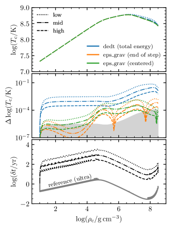
Figure 9: Convergence tests of the evolution of the central quantities for the contracting 1.3 $\mathrm{M}_{\odot}$ sphere of pure carbon using different forms of the energy equation. The central density is a proxy for time. The top panel shows $T_{\rm c}$. The middle panel shows the $T_{\rm c}$ difference from a reference solution. The three line styles represent the three levels of resolution as indicated by the legend in the top left corner of the upper panel. The grey region marks the level of agreement between the set of reference solutions. The lower panel shows the time step for each resolution, with the time step of the runs used in the ultra-resolution reference set indicated as the solid grey line.

Figure 9 shows the trajectory of $T_{\rm{c}}$ versus $\rho_{\rm{c}}$. While this calculation does not consider nuclear reactions, in calculations that do, the $T$ and $\rho$ sensitivity of the nuclear reaction rates motivates obtaining solutions that are converged in these quantities (e.g. Schwab et al. 2015). This example does include thermal neutrinos, which lead to central cooling at high density. The top panel shows that the two eps_grav versions agree (to within the line width) at all resolutions, while the dedt form shows visible differences during the evolution after the model has reached its maximum $T_{\rm{c}}$. The level of difference from the reference solution is shown in the middle panel. All forms exhibit first-order convergence, where a 1 dex reduction in the time step leads to a 1 dex reduction in the error in $T_{\rm{c}}$. However, at a fixed resolution, the eps_grav forms show similar performance to each other and superior performance relative to the dedt form.

In order to understand why the eps_grav forms perform better under degenerate conditions, consider an adiabatic change, ${\mathrm{d}e+P\mathrm{d}(1/\rho)=T\mathrm{d}s=0}$ at fixed composition. This expression is satisfied exactly for infinitesimal changes and a perfect EOS. When we integrate across a time step, we know the integral of total time derivatives (e.g. ${\mathrm{D}e/\mathrm{D}t}$ or ${\mathrm{D}\ln\rho/\mathrm{D}t}$) exactly, but approximate the integral over the time step for quantities that are not total time derivatives. The extent to which our scheme will fail to reproduce an adiabatic evolution is the error in approximating these other integrated quantities appearing in the energy equation (e.g., $P$ or $c_{V}$). Recall that the usual backwards Euler approach in MESA is effectively like assuming that the non-total-time-derivative part is constant and equal to the end-of-time step value (e.g., $P=P_{\rm end}$).

For nearly adiabatic evolution in electron degenerate conditions, we have a cancellation between large $\mathrm{d}e$ and ${P\mathrm{d}(1/\rho)}$ terms, but this cancellation ends up incomplete in MESA because the evaluation of the former term is exact while the latter has error. The error is usually small compared to the order of the terms being subtracted, and so imperfect cancellation often will not introduce large errors. But in degenerate material, the scale of the cancelling terms is larger than the thermal energy by roughly the degeneracy parameter ${\eta\equiv\mu_{e}/k_{\rm B}T}$, where $\mu_{e}$ is the electron chemical potential. Therefore, otherwise small cancellation errors can be amplified by a factor of $\eta$ for the temperature evolution.

By contrast, when we write the $\epsilon_{\rm grav}$ form, this cancellation for adiabatic evolution instead occurs in ${[\rho(\partial e/\partial\rho)_{T}-P/\rho]}$ (Equation 51) which is replaced with ${c_{P}T\nabla_{\rm ad}\chi_{\rho}}$ in the form of Equation (52) that MESA uses for its eps_grav implementation. This captures adiabatic density evolution in terms of EOS derivative quantities that are not subject to cancellation errors. Instead, accuracy in this form is limited by the accuracy of our approximations over finite time steps for thermodynamic quantities like $\nabla_{\rm ad}$ appearing in the energy equation. The error associated with time discretization, $[c_{P}T(1-\nabla_{\rm ad}\chi_{T})]_{\rm end}\Delta\ln T+[c_{P}T\nabla_{\rm ad}\chi_{\rho}]_{\rm end}\Delta\ln\rho$, is at least a factor of $\sim\eta$ smaller than the cancellation error, and in practice can be even better.

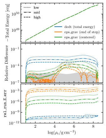
Figure 10: Convergence tests of the evolution of the total energy for the contracting 1.3 $\mathrm{M}_{\odot}$ sphere of pure carbon using different forms of the energy equation. The top panel shows the negative total energy. The middle panel shows the difference from a reference solution. The grey region marks the level of agreement between the set of reference solutions. The lower panel shows the relative cumulative energy error for each run.

Figure 10 shows the total energy of the model. The top panel shows that all runs agree in this quantity within the line width, while the middle panel reveals the level of relative difference. We emphasize that even though the dedt runs report by far the best cumulative energy error as a measure of step-to-step internal energy consistency (lower panel of Figure 10), they nevertheless show less accurate evolution of the total energy and temperature relative to the ultra high-resolution reference runs (middle panel of Figure 10). This is because the cumulative energy error reports the degree to which energy is conserved by evolution steps, while the total energy is a function of the global stellar structure which can slowly diverge even with zero reported energy error. This reflects the fact that “energy error” as reported by MESA is primarily a measure of the internal consistency of the stellar structure solver, and should not be construed as always reflecting globally accurate energy evolution. This reported error is still a useful diagnostic for MESA models, but must be interpreted with caution.

All forms of the energy equation in Figure 10 approximately show first-order convergence in the total energy. The lower panel shows that the different forms exhibit notably different behaviors with increasing time resolution. The dedt form has excellent numerical energy conservation that does not depend on time resolution. The error is roughly the error due to the non-zero residuals in the solution of the energy equation. The eps_grav forms display worse performance in this quantity, though the error shrinks as the time step decreases. The “end of step” form shows first-order convergence, while the “centered” variant exhibits more rapid, second-order convergence with smaller numerical energy conservation errors at fixed resolution. We would expect these trends to continue until the numerical energy conservation error is no longer dominated by errors due to the temporal discretization, at which point it reaches the floor set by non-zero residuals or imperfect EOS thermodynamics.

The pure carbon case shows that the time-centered eps_grav form of the energy equation is the best choice for models evolving under degenerate conditions, with the best balance between accurate temperature evolution and step-to-step energy conservation according to Figures 9 and 10. This case was idealized to focus on the effects of finite equation residuals and time discretization. We now move on to discussing the additional complexities introduced by EOS imperfections.

5.3 Quantifying EOS shortcomings

The value of $e$ returned by the EOS is an essential ingredient in evaluating the total energy of the model, and high-quality partial derivatives of EOS quantities are critical for accurate and efficient solver performance. We now discuss three primary EOS issues that influence energy conservation and solver performance. First, an EOS may return low quality partial derivatives that degrade convergence of the implicit solver. We now mitigate this with more careful derivative accounting described in §5.3.1. Second, an EOS may have internal inconsistencies in its reported thermodynamics. We have mitigated this by upgrading the MESA EOS patchwork with Skye (Jermyn et al., 2021) and FreeEOS (Irwin, 2004) as described in §4. Third, even when individual EOS components yield excellent thermodynamic consistency, the necessity of blending between EOS components to provide continuous coverage across different regimes inevitably introduces additional thermodynamic inconsistency. We have mitigated this last issue by minimizing the number and severity of EOS blends as much as possible, but unavoidable energy inconsistencies remain, and we discuss their implications for energy conservation in §5.3.2.

5.3.1 EOS Derivatives

In MESA V, we addressed the quality of the EOS derivatives by introducing new options that used bicubic spline interpolation in high-resolution tables of $P_{\rm{gas}}$, $s$, and $e$. This provided accurate first and second partial derivatives by evaluating analytic derivatives of the interpolating polynomials rather than by interpolating values of tabulated derivatives. While this approach successfully ensured that the partial derivatives corresponded to how the interpolated EOS values actually changed in response to small changes of the parameters, it inevitably led to small, interpolation-related artifacts in partial derivative quantities such as $\nabla_{{\rm ad}}$ or $\Gamma_{1}$. In asteroseismic applications that require smooth profiles of the Brunt-Väisälä frequency, this approach proved unsatisfactory.

MESA now adopts an approach that separately treats quantities that appear in the equations (and happen to be partial derivatives) and the places where these theoretically equivalent, but numerically different quantities appear in the Jacobian (as partial derivatives of other quantities that appear in the equations). That is, the Jacobian uses the partial derivatives of bicubic spline interpolants, while the equations use the bicubic spline interpolants of partial derivatives. This enables both efficient numerics and smoother solutions at the cost of some additional bookkeeping. A potential pitfall is that negative values for non-negative quantities can be encountered. In practice, we find that we do not encounter negative interpolants for the physical quantities that enter the equations. While we may encounter negative values from the derivatives of the interpolants used for the Jacobian, these only guide the Newton iterations in converging toward a solution. In this scheme, negative derivatives of interpolants cannot introduce physical errors into the equations used for model solutions.

5.3.2 Thermodynamic Consistency and EOS Blends

In order to quantify how models employing the different forms of the energy equation experience inconsistencies in the EOS differently, we establish a measure of the quality of the MESA EOS during the evolution of a model as follows. In the $(\rho,T,\{X_{i}\})$ basis, the total derivative of the specific internal energy, $e$, mathematically satisfies

$$\begin{split}\frac{\mathrm{D}e}{\mathrm{D}t}-&\left[\left(\frac{\partial e}{\partial\rho}\right)_{T,\{X_{i}\}}\frac{\mathrm{D}\rho}{\mathrm{D}t}+\left(\frac{\partial e}{\partial T}\right)_{\rho,\{X_{i}\}}\frac{\mathrm{D}T}{\mathrm{D}t}\right.\\ &\left.\;\;+\sum_{i}\left(\frac{\partial e}{\partial X_{i}}\right)_{\rho,T,\{X\neq X_{i}\}}\frac{\mathrm{D}X_{i}}{\mathrm{D}t}\right]=0.\end{split}$$ (55)

For a Lagrangian volume corresponding to a cell $k$, we evaluate the time integral of the left hand side of Equation (55) across a time step. We replace the sum over individual composition derivatives with a single directional derivative along the direction of composition change over the time step, as in the evaluation of $\epsilon_{{\rm grav},X_{i}}$. We approximate terms that are not the integral of total derivatives using the implicit trapezoidal rule. Weighting by $dm_{k}$ and summing over all cells this gives, for a single step,

$$\begin{split}E_{\rm err,eos}^{\rm step}=\sum_{k=1}^{n}dm_{k}\Bigg{\{}\Delta e&-\overline{\left[\rho\left(\frac{\partial e}{\partial\rho}\right)_{T}\right]}\Delta\ln\rho\\ &-\overline{[c_{V}T]}\Delta\ln T-\overline{\Delta e_{X_{i}}}\Bigg{\}}_{k}~{},\end{split}$$ (56)

where overline quantities are the trapezoidal rule estimates corresponding to the average at the start and end of the time step. The value $\Delta e_{X_{i}}=e(\{X_{i}\})-e(\{X_{i}\}_{\rm start})$ is the change in specific internal energy due to composition changes alone at a given $\rho$ and $T$, so

$$\begin{split}\overline{\Delta e_{X_{i}}}=\frac{1}{2}\big{[}&e(\rho_{\rm start},T_{\rm start},\{X_{i}\})-e(\rho_{\rm start},T_{\rm start},\{X_{i}\}_{\rm start})\\ &+e(\rho,T,\{X_{i}\})-e(\rho,T,\{X_{i}\}_{\rm start})\big{]}~{}.\end{split}$$ (57)

Summing the per-step errors over a MESA run, then at the $n$-th time step, we have

$$E_{\rm err,eos}^{\rm run}=\sum_{i=1}^{n}E_{\rm err,eos}^{{\rm step},i}.$$ (58)

As the time step is reduced, the error from the temporal discretization shrinks and $E_{\rm err,eos}^{\rm run}$ converges to a measure of the energy error incurred as a result of EOS shortcomings.

We define two other energy errors. By limiting the sum in Equation (56) to those zones that are in an EOS blend during a particular time step, we can isolate the per-step energy error due to the blend and so analogously define $E_{\rm err,blend}^{\rm step}$ and $E_{\rm err,blend}^{\rm run}$. We define the per-step residual energy error $E_{\rm err,res}^{\rm step}$ as the mass-weighted sum of the energy equation residuals over the model and also track its cumulative value $E_{\rm err,res}^{\rm run}$.

To understand how these different forms of error might manifest under different treatments of the energy equation, it is helpful to consider the idealized case of an EOS that is a blend of EOS1 and EOS2, identical except for their definition of where the energy zero point lies, so that ${e_{\rm EOS1}=e_{\rm EOS2}+e_{\rm offset}}$, where $e_{\rm offset}$ is some constant. Physically, either EOS should produce the same evolution, and all EOS derivatives will be the same. However, evolution through the blend between EOS1 and EOS2 will not satisfy Equation (55), and therefore must lead to non-zero values of $E_{\rm err,eos}^{\rm step}$ regardless of which form of the energy equation is used. In particular, the thermodynamic identity ${c_{V}=(\partial e/\partial T)_{\rho}}$ is violated in the blending region because the blending coefficient derivatives are not included as part of the blended value of $c_{V}$ (see §4.3).

In practice, such energy offsets (in addition to other inconsistencies) always occur at the locations of MESA EOS blends because it is impossible to construct a blending region in which two distinct EOS treatments agree exactly. Due to different input physics assumptions in different EOS components, energy offsets have more complexity than simple constant zero point differences across the range of parameters where blending is necessary. As far as possible, we have chosen blending locations to minimize the differences between EOS components and to minimize the residual amount of unavoidable offset (e.g., by adjusting the definitions of internal energy to be as consistent as possible about where the zero point lies). However, no general solution is currently available to completely eliminate inconsistencies for blends between our current EOS components, and EOS blends therefore remain one of the largest potential sources of energy error when present in MESA models.

When evolving using the dedt form of the energy equation, Equation (49) will lead to $e_{\rm offset}$ being folded into the $\mathrm{D}e/\mathrm{D}t$ term of the energy equation for regions of the model evolving through the blend, injecting spurious heating/cooling into those regions. However, the energy error reported by MESA in these regions may still be 0, because MESA evaluates energy error according to the blended $e$ from the EOS. It is therefore possible to have models for which $E_{\rm err,eos}^{\rm step}$ is significantly larger than E_err reported by MESA when using the dedt form of the energy equation, as we shall see in the following subsection. On the other hand, in this idealized scenario the eps_grav form of the energy equation (Equations 51 and 52) would give the physically correct evolution since it is evaluated in terms of derivatives that are unaffected by the energy offset in the blending region. However, both $E_{\rm err,eos}^{\rm step}$ and rel_run_E_err will report large values under the eps_grav form in this scenario, reflecting the thermodynamic inconsistency of $e$ in the blended EOS rather than inaccuracy in the evolution.

5.4 Results: 1M_pre_ms_to_1TP

Having demonstrated the performance of the various forms of the energy equation in idealized circumstances in §5.2, we now model the evolution of a 1 $\mathrm{M}_{\odot}$ star from the pre-main sequence to its first He thermal pulse on the AGB. This example includes composition changes due to nuclear reactions, and it uses the current default MESA EOS (blending together FreeEOS and Skye for the $(\rho,T)$ regions encountered by this model). A small portion of the envelope of this model encounters the FreeEOS-OPAL/SCVH blend near ZAMS, then the model lies entirely on FreeEOS for most of the first $\approx$5 Gyr of MS evolution (see §4 and Figure 7), after which the core evolves toward higher density and encounters the FreeEOS-Skye blend. The approach described in §5.3 allows us to quantify the various sources of energy errors, identifying how much error comes from EOS inconsistencies and blends, and how much is due to residuals of the equation solutions.

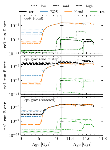
Figure 11: Comparison of types of energy errors for a 1 $\mathrm{M}_{\odot}$ model. Each panel shows a different form of the energy equation. Each line color indicates a different type of energy error. Each line style indicates a different time resolution. The thick black lines show the error in numerical energy conservation that MESA reports as rel_run_E_err. The thinner colored lines show the errors due to the EOS, EOS blends, and equation residuals. The composition term $\epsilon_{{\rm grav},X_{i}}$ is included for both of the eps_grav panels in this figure.

Figure 11 summarizes the energy errors defined in §5.3 when using different forms of the energy equation. Because the models are approximately converged and the different forms of the energy equation converge to the same solution, the colored lines at a given time resolution are similar in all panels. In particular, the measure of the energy error associated with the EOS blend has approximately converged (agreement among orange lines in the middle of each panel). However, the measure of the EOS inconsistency in places where this quantity is not dominated by the blend (i.e., where the blue lines are above the orange lines) continues to shrink with increasing time resolution, showing that this measure is not converged and that the true inconsistency is less than that indicated by the highest resolution line.

In the top panel, the dedt form shows a numerical energy error (black lines) that is roughly the energy error associated with the equation residuals (green lines). The EOS energy errors are present in the model, but do not show up in the reported rel_run_E_err for this form of the energy equation, as explained in §5.3. In the middle panel, the end-of-step eps_grav form shows that the numerical energy conservation error remains above the energy errors associated with the EOS, while these in turn are generally well above the errors associated with the equation residuals. In the bottom panel, the centered eps_grav form shows a numerical energy error (black lines) that is roughly the energy error associated with the EOS inconsistencies. In particular, by the end of the main sequence, the numerical energy error is dominated by the blend error. Further resolution increases or improvements to the energy equation will not improve the numerical energy conservation. Progress can only come through improvements to the EOS.

6 Atmosphere

The MESA atm module uses an atmosphere model to evaluate the pressure $P_{\rm s}$ and temperature $T_{\rm s}$ at the outermost ($k=1$) cell boundary. These ‘model surface’ values are in turn incorporated in the outer boundary conditions applied to the stellar model, as specified in Equation (10) of MESA I. Here we describe various improvements and fixes in the atm module since MESA I and MESA II.

In older MESA releases, the choice of atmosphere model was controlled by the which_atm_option inlist parameter. In recent releases this parameter is renamed atm_option, with three possible choices:

• atm_option = 'T_tau': atmosphere based on $T(\tau)$ relations, as discussed in §6.1.

• atm_option = 'irradiated': irradiated atmosphere, as discussed in §6.2.

• atm_option = 'table': tabulated atmosphere, as discussed in §6.3.

In addition, MESA now offers two complementary approaches to including the atmosphere structure in model data passed as input into pulsation codes. These are described in §6.4 and §6.5.

6.1 Atmospheric $T(\tau)$ Relations

Setting atm_option = 'T_tau' builds an atmosphere in which temperature at each optical depth $\tau$ is specified by a function $T(\tau)$; $P_{\rm s}$ and $T_{\rm s}$ are obtained by evaluating the atmospheric thermodynamic state at an optical depth $\tau_{\rm s}$ corresponding to the nominal model surface. This optical depth can be much smaller or much greater than the optical depth $\tau\approx 2/3$ typically associated with stellar photospheres; that is, the model surface need not correspond to the photosphere.

The $T(\tau)$ functions have the form

$$T^{4}(\tau)=\frac{3}{4}T_{\rm eff}^{4}\left[\tau+q(\tau)\right].$$ (59)

Selection of $T(\tau)$ is set by the atm_T_tau_relation inlist parameter, with four possible choices:

• atm_T_tau_relation = 'Eddington': the gray, Eddington-approximation relation, where $q(\tau)=2/3$.

• atm_T_tau_relation = 'solar_Hopf': the $q(\tau)$ function described in Equation (A9) of MESA II, which is a fit to Model C of the solar atmosphere by Vernazza et al. (1981), often referred to as VAL C.

• atm_T_tau_relation = 'Krishna_Swamy': the relation from Equation (33) of Krishna Swamy (1966).

• atm_T_tau_relation = 'Trampedach_solar': the relation from Ball (2021), itself a fit to the solar atmosphere simulation by Trampedach et al. (2014).

For a given $T(\tau)$ relation, the corresponding $P(\tau)$ throughout the atmosphere is obtained by integrating the hydrostatic balance equation

$$\frac{\partial P}{\partial\tau}=\frac{g}{\kappa},$$ (60)

from $\tau\ll 1$ inward to $\tau=\tau_{\rm s}$. In this integration the gravity is set to the constant value $g=GM/R^{2}$, in accordance with the assumption that the atmosphere is geometrically thin and contains negligible mass. The opacity evaluation is controlled by the atm_T_tau_opacity inlist parameter, with three possible choices:

• atm_T_tau_opacity = 'fixed' — uniform $\kappa$ throughout the atmosphere, with a value set by the current opacity $\kappa_{1}$ in the outermost cell.

• atm_T_tau_opacity = 'iterated' — uniform $\kappa$ throughout the atmosphere, with a value obtained from the kap module for $(P_{\rm s},T_{\rm s})$. As indicated by its name, this choice requires iteration because $P_{\rm s}$ is not known a priori.

• atm_T_tau_opacity = 'varying' — varying $\kappa$ throughout the atmosphere, with a value obtained from the kap module for $(P,T)$ at the local $\tau$.

With the last choice, the dopri5 ($5^{\rm th}$-order Dormand-Prince) differential equation integrator from the num module is employed with specifiable error tolerance and maximum number of steps. With the first and second choices, however, the fact that $\kappa$ does not depend on $\tau$ means that Equation (60) can be integrated analytically to yield

$$P(\tau)=\frac{g}{\kappa}\tau\left(1+\texttt{Pextra\_factor}\times\frac{\kappa L}{6\pi GMc\tau}\right).$$ (61)

The second term in the parentheses arises as a constant of integration, and accounts for non-zero radiation pressure in the limit of small $\tau$. The term is obtained from Equation (20.16) of Cox & Giuli (1968). The parameter Pextra_factor depends on the assumed angular dependence of the radiation specific intensity, with the default value of unity corresponding to isotropic-outward, and a value of $1.5$ corresponding to radial-outward. While unphysical, setting $\texttt{Pextra\_factor}>1.5$ can sometimes be a useful numerical strategy to improve convergence in models that are close to the Eddington limit. However, caution is warranted as this strategy can produce incorrect stellar radii.

Release r11701 and earlier	Release r12115 and later
which_atm_option	atm_T_tau_relation	atm_T_tau_opacity
'simple_photosphere'	'Eddington'	'fixed'
'gray_and_kap'	'Eddington'	'iterated'
'Eddington_gray'	'Eddington'	'varying'
'Krishna_Swamy'	'Krishna_Swamy'	'varying'
'solar_Hopf'	'solar_Hopf'	'varying'

Table 5: Mapping between which_atm_option parameter choices in releases of MESA up to r11701 (see §12.4), and the corresponding parameter choices in releases since r12115 (to be used in tandem with atm_option = 'T_tau').

For $T(\tau)$ atmospheres, Table 5 summarizes the mapping between the which_atm_option parameter choices supported in older MESA releases, and the combinations of atm_T_tau_relation and atm_T_tau_opacity parameter choices that provide the replacement functionality.

In implementing the changes described here, we uncovered two issues that impacted the accuracy and performance of the atm module in older releases.

First, calls to the eos and kap modules to evaluate $\rho(P,T)$ and $\kappa(\rho,T)$ did not use the same tables and/or configuration options as the interior model, leading to possible inconsistencies at the surface where the atmosphere and the interior join. To fix this problem, we implemented a callback system so that the star module can pass appropriately configured EOS and opacity wrapper routines to the atm module.

Second, in cases where atm_T_tau_opacity = 'iterated', the partial derivatives of $P_{\rm s}$ and $T_{\rm s}$ with respect to dependent variables ($L_{1},r_{1},\rho_{1},T_{1}$) in the outermost cell were incorrectly evaluated; in some cases, this caused the global Newton solver to converge slowly or not at all. To fix this problem, we implemented the correct expressions, which follow from application of the chain rule to the $T(\tau)$ relation and the hydrostatic solution (Equation 61).

6.2 Irradiated Atmospheres

Setting atm_option = 'irradiated' provides functionality similar to 'T_tau', but adopting the $T(\tau)$ relation for an externally irradiated atmosphere given in Equation (6) of Guillot & Havel (2011). Equation (60) is integrated analytically, with opacity evaluation controlled by the atm_irradiated_opacity inlist parameter; the possible choices 'fixed' and 'iterated' behave the same as described in §6.1. The 'iterated' case replaces the which_atm_option = 'gray_irradiated' choice described in MESA II, and fixes a bug related to incorrect $T_{\rm eff}$ evaluation.

6.3 Tabulated White Dwarf Atmospheres

When atm_option = 'table', $P_{\rm s}$ and $T_{\rm s}$ are obtained by interpolating in pre-computed atmosphere tables. In addition to the options described in MESA I and MESA II, MESA now provides a new set of atmosphere tables for WDs with He-dominated surfaces (DB WDs). These tables provide $P_{\rm s}$ and $T_{\rm s}$ data over the ranges $5,000\,\mathrm{K}<T_{\rm eff}<40,000\,\mathrm{K}$ and $6.0<\log(g/\mathrm{c}\mathrm{m}\,{\mathrm{s}}^{-2})<9.4$. They assume a He dominated composition of $n_{\rm{H}}=10^{-5}n_{\rm{He}}$, and are based on model atmospheres calculated using the Koester (2010) code and evaluated at $\tau=25$. The limits of this grid are now explained.

At $T_{\rm eff}\gtrsim 40,000$ K He undergoes its second ionization, and non-LTE effects that are not included in the atmosphere code become important. The lower limit of $T_{\rm eff}=5,000\,\mathrm{K}$ is imposed by the Koester (2010) code’s EOS. Studies of spectroscopic samples of DBs (e.g., Eisenstein et al., 2006; Genest-Beaulieu & Bergeron, 2019) have shown that DBs are well described for surface gravities lower than $\log(g/\mathrm{c}\mathrm{m}\,{\mathrm{s}}^{-2})=9.5$. The lower limit of $\log(g/\mathrm{c}\mathrm{m}\,{\mathrm{s}}^{-2})=6.0$ is imposed by the convergence of the models at $T_{\rm eff}=40,000\,\mathrm{K}$, since radiation pressure competes with gravity in this regime.

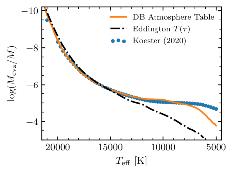
Figure 12: Depth of the surface convection zone (measured as fractional convection zone mass $M_{\rm cvz}/M$) for a $0.57\,\mathrm{M}_{\odot}$, $\log(g/{\rm cm\,s^{-2}})\approx 8.0$ WD with a He atmosphere. The curves indicate MESA results with the DB tables and the Eddington $T(\tau)$ relation, while the points are based on Koester et al. (2020).

As a diagnostic for these new tables, we use the depth of the surface convection zone in cooling DB WD models, which is primarily sensitive to the atmospheric boundary condition and the stellar model EOS in the convective region. Figure 12 demonstrates the improvements brought by these new tables, plotting the mass $M_{\rm cvz}$ of the surface convection zone versus $T_{\rm eff}$. Also shown are results from the atmosphere and envelope models of Koester et al. (2020), as well as the outcome from using atm_option = 'T_tau' with atm_T_tau_relation = 'Eddington' and atm_T_tau_opacity = 'fixed'.

The new tables reproduce the Koester et al. (2020) calculations much better at low $T_{\rm eff}$ than the Eddington $T(\tau)$ atmospheres. The latter diverge for $T_{\rm eff}\lesssim 15,000\,\mathrm{K}$ because the conditions at the surface cross the boundaries of the He opacity table coverage in MESA. The tabulated atmospheres agree with Koester et al. (2020) to $T_{\rm eff}\approx 7,000\,\mathrm{K}$. For cooler temperatures, the uncertainty in $M_{\rm cvz}$ is due to the uncertain EOS at the base of the convection zone (Saumon et al., 1995).

6.4 Atmosphere Reconstruction for Pulsation Codes

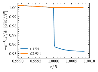
Figure 13: The hydrostatic term $\rho^{-1}{\mathrm{d}}P/{\mathrm{d}}r$ (in units of the surface gravity $GM/R^{2}$) as a function of $r/R$ for GYRE-format models of the present-day Sun that include reconstructed atmospheres with atm_option = 'T_tau', atm_T_tau_relation = 'Eddington' and atm_T_tau_opacity = 'varying'. The two curves show releases r11701 (prior to the reconstruction fix) and r22.05.1; only the latter reproduces the correct behavior $\rho^{-1}{\mathrm{d}}P/{\mathrm{d}}r=-GM/R^{2}$ throughout the reconstructed atmosphere $r/R\geq 1$.

As discussed in MESA II and MESA III, MESA can pass models to the ADIPLS (Christensen-Dalsgaard, 2008) or GYRE (Townsend & Teitler, 2013) linear pulsation codes, either in-memory during an astero-module optimization or via files written to disk in a variety of formats. Often, it is desirable to reconstruct the atmosphere structure from $\tau=\tau_{\rm s}$ out to $\tau\ll 1$ before passing them to the pulsation codes. This has no impact on the interior model, but can improve asteroseismic modeling.

For $T(\tau)$ atmospheres (§6.1), setting add_atmosphere_to_pulse_data = .true. enables this reconstruction. The radial coordinate $r$ throughout the atmosphere is then determined by integrating the $\tau$ equation

$${}\frac{\partial r}{\partial\tau}=-\frac{1}{\kappa\rho}$$ (62)

outward from $\tau=\tau_{\rm s}$ to $\tau\ll 1$. For this integration, $\kappa$ is evaluated in accordance with the atm_T_tau_opacity parameter discussed previously, while $\rho(P,T)$ is obtained from the eos module for the local $\tau$.

In releases of MESA prior to r12115, the outward integration used an explicit Euler scheme with a default step-size too large to accurately follow $r(\tau)$. Together with the eos/kap table inconsistency highlighted in §6.1, this led to departures from hydrostatic balance in the reconstructed atmosphere, as highlighted in Figure D.1 of Christensen-Dalsgaard et al. (2020) for $r/R>1$. To fix this issue, release r12115 and later use the dopri5 integrator for the outward integration, with a specifiable error tolerance, step-size and outermost optical depth. Figure 13 demonstrates these improvements by showing hydrostatic balance for GYRE-format models of the present-day Sun calculated using releases r11701 (pre-fix) and r22.05.1.

6.5 Atmospheres as Part of the Interior

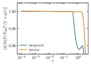
Figure 14: Ratio of the left- and right-hand sides of Equation (59), by which we compare the temperature structure of two models in FGONG format, one with the atmosphere reconstructed as in §6.4 (integrated) and the other with the atmosphere modeled with the interior as in §6.5 (interior).

The optically-thin outer layers of a star are usually treated separately from the interiors of stars because they do not satisfy the assumptions under which the interior structure equations are derived. Given a $T(\tau)$ relation, however, it is possible to correct the equation for radiative heat transport so that the temperature stratification produced by solving the stellar structure equations matches the desired $T(\tau)$ (Trampedach et al., 2014; Mosumgaard et al., 2018a). The radiative temperature gradient $\nabla_{\mathrm{atm}}$ of an atmosphere that follows a given $T(\tau)$ relation is

$$\nabla_{\mathrm{atm}}=\nabla_{\mathrm{rad}}\left(1+\frac{\mathrm{d}q}{\mathrm{d}\tau}\right).$$ (63)

We can therefore recover any $T(\tau)$ relation by scaling the canonical $\nabla_{\mathrm{rad}}$ by $1+\mathrm{d}q/\mathrm{d}\tau$. This procedure is enabled with the new option use_T_tau_gradr_factor. For the gray, Eddington-approximation relation, $q(\tau)$ is constant and no correction is necessary.

To include the optically thin layers in the interior model, the surface boundary should be set or relaxed to a smaller $\tau$ using the flags set_tau_factor or relax_tau_factor and their associated controls. The surface boundary conditions, now at smaller $\tau$, still follow §6.1. They are evaluated at $\tau_{\rm s}=$ tau_factor$\times\tau_{\mathrm{eff}}$ rather than $\tau_{\mathrm{eff}}$, where $\tau_{\mathrm{eff}}$ is the optical depth at which the $T(\tau)$ relation is equal to $T_{\rm eff}$.

This approach has several advantages. First, like atmospheres reconstructed with atm_T_tau_opacity = 'varying', the atmospheric structure is kept consistent with MESA’s EOS and opacity routines. Second, the computation can leverage the parallelization of MESA. Finally, this approach accounts for the fact that $g$ is not exactly constant throughout the atmosphere (§6.4), which is assumed by $T(\tau)$ atmospheres.

Figure 14 shows the ratio of the left- and right-hand sides of Equation (59) in a $1\mathrm{M}_{\odot}$ ZAMS model with the 'solar_Hopf' $T(\tau)$ relation when the atmosphere is either reconstructed as in §6.4 or included as part of the interior. Both models deviate at $\tau\gtrsim 2$ because convection starts to transport heat.

The reconstructed atmosphere deviates in $\tau_{\mathrm{eff}}<\tau\lesssim 2$ because $\mathrm{d}q/\mathrm{d}\tau\neq 0$ just below the photosphere, which is treated as part of the interior without correcting $\nabla_{\rm{rad}}$. When using analytic $T(\tau)$ relations, this can be corrected by using the use_T_tau_gradr_factor option but not when using tabulated atmospheres, for which the correction factors $1+\mathrm{d}q/\mathrm{d}\tau$ have not been provided. Though inconsequential for tables at $\tau_{\rm s}\gg 1$, where $\mathrm{d}q/\mathrm{d}\tau\to 0$ anyway, it introduces inaccuracy in the temperature stratification when using tables at small $\tau$. This inaccuracy may be acceptable, depending on the scientific problem. This inaccuracy is not present if $\mathrm{d}q/\mathrm{d}\tau=0$ in the affected regions, which includes the Eddington $T(\tau)$ relation.

6.6 Choosing atmosphere options

There is limited consensus on when to use which atmosphere options, but we nevertheless offer a few guiding remarks.

The most commonly used and current default in MESA is a gray Eddington atmosphere with the surface boundary at $\tau_{\rm s}=2/3$, with $\kappa$ fixed throughout the atmosphere. If the precise behavior of the stellar atmosphere is not important, this should suffice.

There is a hierarchy of accuracy at the expense of greater computational cost among the choices for atm_T_tau_opacity. On the basis of the self-consistency of $\kappa$, 'varying' is more accurate than 'iterated', which is in turn more accurate than 'fixed'.

For the calculation of pulsations that have significant amplitude near the surface (e.g., solar p modes), it is important to choose an option that allows the atmosphere to be reconstructed for the equilibrium stellar model (§6.4).

Tabulated atmospheres provide boundary conditions that are typically computed using more complete physics (e.g., non-LTE) than can be described by the stellar structure equations. As shown in Figure 14, tabulated atmospheres at $\tau\lesssim 2$ lead to a stellar model in which the near-surface temperature stratification is equivalent to an Eddington atmosphere. The models in Figure 14 differ by $\sim 50$ K at $\tau_{\rm{eff}}$. This inaccuracy might be outweighed by the benefits of a complete atmosphere model. The correct structure could in principle be recovered by extracting the appropriate $T(\tau)$ relations (Trampedach et al., 2014) from the detailed atmosphere models, but these are not generally available.

Ideally, we would have access to grids of $T(\tau)$ relations and corresponding bolometric corrections extracted from advanced simulations of stellar atmospheres, with parameters that cover the HR diagram. Until this ideal is realized, stellar modellers must decide which aspects of the atmospheric boundary condition are most important for their calculations and choose appropriate options.

7 Convection in the Outer Layers of Stars

7.1 Starspots

Starspots are common for stars with $M\lesssim\mathrm{M}_{\odot}$. Models of M dwarfs that include starspots and surface magnetism have inflated radii close to those inferred by observation (e.g., Feiden & Chaboyer 2013; Mann et al. 2015).

We thus implement in MESA the treatment of starspots introduced in the SPOTS models of Somers et al. (2020) (also see Cao & Pinsonneault 2022), which are based on the Yale Rotating Stellar Evolution Code (YREC; Demarque et al. 2008; Spada et al. 2013) and described in detail in Somers & Pinsonneault (2015) and Somers et al. (2020).

7.1.1 Starspots formalism

Somers et al. (2020) parameterize the variance of the surface flux due to magnetic pressure from starspots by modifying the atmospheric boundary condition. Somers & Pinsonneault (2015) characterized the degree of “spottiness” on the stellar surface by two parameters:

1. SPOTF (hereafter $f_{\text{spot}}$), a coverage fraction, or “spot filling factor”

2. SPOTX (hereafter $x_{\text{spot}}$), representing the temperature contrast between the spotted and unspotted regions at $r=R$: $x_{\text{spot}}=T_{\text{spot}}/T_{\text{photosphere}}$.

Numerically, values from $0.0$ to $1.0$ are permitted for both parameters. Observationally constrained coverage fractions $f_{\text{spot}}$ are described in Cao et al. (2022), who find that a value $f_{\text{spot}}=0.34$ is a reasonable fit to observations of sub-solar-mass stars in the $\lambda$ Ori cluster.

The spot-induced temperature contrast, $x_{\text{spot}}$, is restricted to physically meaningful values of $0.5-1.0$. A value of $x_{\text{spot}}=1.0$ indicates that the effective temperature in the spotted region, $T_{\text{spot}}$, does not differ from the surrounding, unspotted effective temperature, $T_{\text{amb}}(r)$ (the “ambient temperature,” or ATEFF in YREC). At the surface, $T_{\text{amb}}(r=R)=T_{\text{photosphere}}$. A value of $x_{\text{spot}}=0.5$, on the other hand, corresponds to the statement that $T_{\text{spot}}$ differs from $T_{\text{amb}}$ by the maximum degree permitted by magnetic equipartition: namely, when the magnetic pressure contribution constitutes half of the total pressure.

The temperature contrast $x_{\text{spot}}$ perturbs the radiative gradient, $\nabla_{\text{rad, spot}}$, in the surface convection zone. This effect can be made depth-dependent via

$$x_{\text{spot}}(r)=1-(1-x_{\text{spot}})\frac{T_{\text{amb}}(r)}{T(r)},$$ (64)

where $T(r)$ is the temperature at $r$ and the quantity $T_{\text{photosphere}}-T_{\text{spot}}=T_{\text{amb}}(R)-T_{\text{spot}}$ is held constant as a function of $r$. In Equation (64), $x_{\text{spot}}$ is a scalar parameter.

Per equations (1) through (4) in Somers & Pinsonneault (2015), the “spotted” luminosity is set to

$$L_{\text{spotted}}\equiv L/\left[f_{\text{spot}}\,x_{\text{spot}}^{4}+(1-f_{\text{spot}})\right].$$ (65)

YREC models the suppression of convective flux at the stellar surface via a two–part lookup in its atmospheric boundary tables, invoking “ambient” versus “spotted” effective temperatures that differ by a factor of

$$\alpha_{\text{spot}}=1+f_{\text{spot}}(x_{\text{spot}}^{4}-1),$$ (66)

where $x_{\text{spot}}$ can optionally be a function of the local temperature at a given depth within the convective envelope.

7.1.2 MESA implementation

MESA’s implementation is equivalent, but modifies the surface boundary conditions in terms of pressure rather than $T_{\rm eff}$, as $T_{\rm eff}$ is strictly an output in MESA. Through the specification of the magnetic pressure term, $P_{\rm{B}}$, the temperature contrast is given by

$$x_{\text{spot}}(r)=\frac{P(r)-P_{\rm{B}}}{P(r)},$$ (67)

where $P_{\rm{B}}$ is assigned at the start of the step via

$$P_{\rm{B}}=(k_{B}N_{A}\rho/\mu)(1-x_{\text{spot}}(R))T_{\rm eff}.$$ (68)

Choosing $x_{\text{spot}}=1$ corresponds to $P_{\rm{B}}=0$, hence there is no magnetic pressure and no perturbation to $P$. Choosing $x_{\text{spot}}=0$ yields the other extreme: $P_{\rm{B}}=P$. Once again, a practical limit on $P_{\rm{B}}$ is set by the assignment $x_{\text{spot}}=0.5$, which corresponds to magnetic equipartition.

Using auto_diff (§2) we account for the modified pressure term and its partial derivatives at every mass shell. In Equations (67) and (68), $P$ and $P_{\rm{B}}$ are auto_diff variables. Likewise, the radiative temperature gradient due to the presence of spots (i.e., magnetic inhibition of the convective flux),

$$\nabla_{\text{rad, spot}}=\nabla_{\text{rad}}/(f_{\text{spot}}\,x_{\text{spot}}(r)^{4}+1-f_{\text{spot}}),$$ (69)

is an auto_diff variable, since it is a function of the auto_diff quantities $\nabla_{\text{rad}}$, $P$, $x_{\text{spot}}(r)$, and scalars.

The quantity $P_{\rm{B}}$ is assigned once at the beginning of every evolutionary step and held constant over all Newton iterations within that step. The use of auto_diff data types ensures that the Newton solver automatically receives correct partial derivatives of the modified radiative temperature gradient with respect to, e.g., depth and other stellar structure variables. The modification to $\nabla_{{\rm rad}}$ is evaluated once per Newton iteration. To obtain the spotted luminosity, $L$ is adjusted by a factor of $\alpha_{\text{spot}}$ (Equation 66).

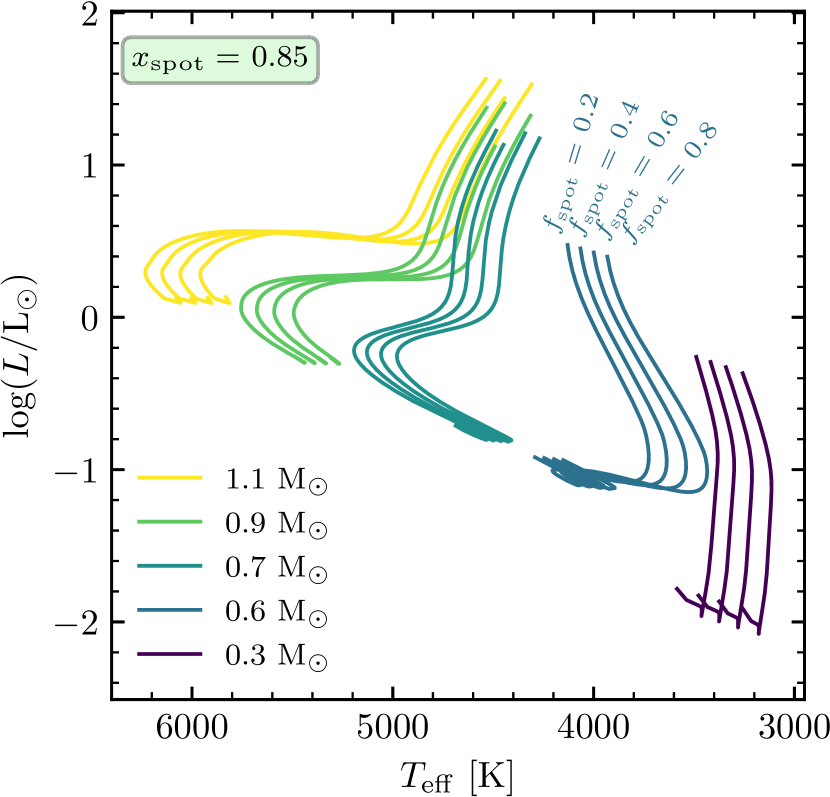
Figure 15: Evolutionary tracks showing the effects of star spots for $x_{\text{spot}}=0.85$. Color indicates mass. Within clusters of identical mass, $f_{\text{spot}}$ values are ordered lowest (left-most) to highest (right-most).

7.1.3 MESA Models

We demonstrate the starspots functionality by computing a grid of spotted evolutionary tracks for $M=0.2-1.3\,\mathrm{M}_{\odot}$ and $\rm{Z}=0.014$. We use the photosphere table option for atmospheric boundary conditions across all tracks, though for the lowest–mass stars (e.g.,  $M\lesssim 0.5\,\mathrm{M}_{\odot}$), a choice of tau_1m1 would be more appropriate. We use the Henyey MLT prescription with $\alpha_{\text{MLT}}=1.95$.

Figure 15 shows tracks using $f_{\text{spot}}=\{0.2,0.4,0.6,0.8\}$ and $x_{\text{spot}}=0.85$. When comparing MESA models to the YREC-based SPOTS models of Somers et al. (2020), we observe the following features:

• Tracks computed with MESA starspots shift smoothly by the same magnitude and in the same direction as a function of $f_{\text{spot}}$.

• We also find that the lower the initial value of $x_{\text{spot}}$ (i.e., more extreme in terms of magnetism), the greater the impact of an increased coverage fraction.

• Below $\approx 0.6\,\rm{M}_{\odot}$, the SPOTS models are cooler than the MESA starspots models. This is due to differences in our choice of the atmospheric boundary condition.

• The degree of radial inflation for an $0.3\,\rm{M}_{\odot}$ M dwarf predicted by MESA starspots, using $f_{\text{spot}}=0.34$ and $x_{\text{spot}}=0.85$, is of the order 3%-5%, in agreement with the SPOTS models.

The MESA starspots test case can be found in MESA_DIR/star/test_suite/starspots.

7.2 Superadiabatic Convection in Radiation-dominated Regions

Modeling stars near the Eddington limit is a complex numerical problem. Under such conditions, convective regions with density inversions are expected (Joss et al., 1973; Paxton et al., 2013) and 1D models using standard MLT can develop extended low-density envelopes, becoming red supergiants before finishing their MS evolution (e.g., Sanyal et al. 2015; Szécsi et al. 2015). Three-dimensional radiative hydrodynamic simulations are just starting to explore the physics of energy transport near the Eddington limit (Jiang et al., 2015; Tsang & Milosavljević, 2015; Schultz et al., 2020; Goldberg et al., 2022; Moens et al., 2022), and will hopefully provide a way to accurately model these regions in 1D stellar evolution instruments. In the meantime, 1D simulations using MLT near the Eddington limit are expensive, requiring small timesteps down to the point that some calculations become impractical. Enhanced convective energy transport in these regions can inhibit the formation of density inversions and facilitate calculations. One such approach is the use of a density scale height rather than a pressure scale height in MLT (Nishida & Schindler, 1967; Stothers & Chin, 1973; Maeder, 1987).

The MLT++ formalism is a stellar-engineering approach that has been commonly used in MESA to reduce superadiabaticity in regions nearing the Eddington limit (MESA III). Although convection is expected to operate in regions of the star approaching the Eddington limit, the efficiency of convective energy transport is uncertain. By reducing the expected superadiabaticity, MLT++ provides an ad-hoc enhancement. Such an enhancement is supported by results from 3D simulations (Jiang et al., 2015; Schultz et al., 2020), but the method is not calibrated to detailed simulations or observations. The main motivation for MLT++ is to enable computations of massive star evolution up to late stages, and users need to assess if the deviations from a more physical model such as MLT are relevant to their results. One important limitation of MLT++ is that it is a non-local explicit method, which can lead to large step-to-step variations that produce unphysical results and prevent the solver from finding a valid solution. By making use of auto_diff (§2), we have implemented a fully implicit and local alternative to MLT++, which allows the modelling of a larger range of masses and metallicities. Setting the option use_superad_reduction activates this method.

In hydrostatic equilibrium, the ratio between the radiative luminosity and the local Eddington luminosity is

$$\Gamma_{\mathrm{Edd}}\equiv\frac{L_{\mathrm{rad}}}{L_{\mathrm{edd}}}=\frac{4aT^{4}}{3P}\nabla.$$ (70)

For a particular model of energy transfer (e.g., TDC as discussed in §3, or MLT), the expected Eddington factor is

$$\Gamma_{\mathrm{Edd,exp}}\equiv\frac{4aT^{4}}{3P}\nabla_{\mathrm{exp}},$$ (71)

where $\nabla_{\mathrm{exp}}$ is the temperature gradient predicted by the energy transfer model. As in MLT++, we artificially enhance energy transport in convective regions where the expected Eddington factor is high by adjusting $\nabla_{\mathrm{rad}}$. The difference between the radiative and the Ledoux gradient is reduced to

$$\nabla_{\mathrm{rad,new}}-\nabla_{\mathrm{L}}=\frac{\nabla_{\mathrm{rad}}-\nabla_{\mathrm{L}}}{f_{\Gamma}},$$ (72)

where $\nabla_{\mathrm{rad,new}}$ is the adjusted radiative temperature gradient and $f_{\Gamma}\geq 1$ determines the reduction of ${\nabla_{\mathrm{rad}}-\nabla_{\mathrm{L}}}$ in the convective region. Such a scaling of $\nabla_{\mathrm{rad}}$ can be interpreted as an effective lowering of $\kappa$ in regions near the Eddington limit. Results from Schultz et al. (2020) suggest that the impact on radiative transfer of a vigorously convecting region supports this choice. The adjusted $\nabla_{\mathrm{rad,new}}$ is then used instead of $\nabla_{\mathrm{rad}}$ to recompute $\nabla$ according to the convection model.

The functional form of $f_{\Gamma}$ is arbitrary, and was determined empirically so that Equation (72) can be applied in a large number of cases while minimizing adjustments in the limit $\Gamma_{\rm Edd,exp}\rightarrow 0$. Just as with MLT++, it serves as a stellar-engineering method to circumvent complex evolutionary stages, rather than a specific physical model that accounts for how convection is modified near the Eddington limit. While exploring different options for $f_{\Gamma}$, auto_diff played a critical role by removing the need to directly specify partial derivatives.

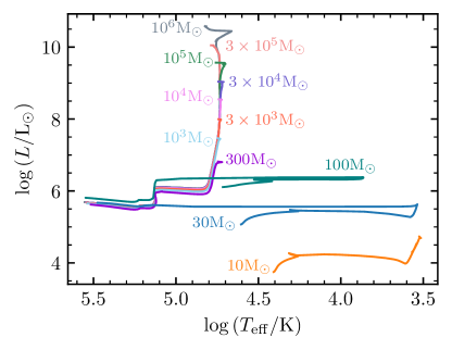
Figure 16: Evolution of stars ranging from 10 to 10⁶ $\mathrm{M}_{\odot}$ at solar metallicity, using the implicit method to increase the efficiency of energy transport in regions approaching the Eddington limit.

Our choice for $f_{\Gamma}$ is the following:

$$\begin{aligned} f_{\Gamma}&=1\\ &+\frac{\alpha_{1}g(\Gamma_{\mathrm{Edd,exp}}/\Gamma_{\mathrm{c}}-1)+\alpha_{2}g(\Gamma_{\mathrm{exp}}/\Gamma_{\mathrm{inv}}-1)}{\sqrt{\beta}}\\ &\times h((\nabla_{\mathrm{exp}}-\nabla_{\mathrm{L}})/\delta_{\rm{c}}),\end{aligned}$$ (73)

where $\beta$ is the ratio of gas to total pressure and $\Gamma_{\mathrm{inv}}\equiv 4(1-\beta)/(4-3\beta)$ is the Eddington factor at which an ideal gas with radiation develops a density inversion (Joss et al. 1973, MESA III). The parameters $\Gamma_{\mathrm{c}}$, $\alpha_{1}$, $\alpha_{2}$ and $\delta_{\rm{c}}$ regulate the enhancement of energy transport. The function

$$g(x)\equiv\begin{cases}0&x<0\\ x^{2}/2&0<x<1\\ x-1/2&x>1\end{cases}$$ (74)

is continuous with a continuous first derivative. No correction will be applied if $\Gamma_{\mathrm{exp}}<\Gamma_{\mathrm{c}}$ and $\Gamma_{\mathrm{exp}}<\Gamma_{\mathrm{inv}}$. If either of those thresholds is exceeded, $\alpha_{1}$ and $\alpha_{2}$ set the strength of the enhancement in energy transport for each. The $1/\sqrt{\beta}$ term further enhances the effect in regions dominated by radiation pressure. The function $h(x)$ is chosen as

$$h(x)=\begin{cases}0&x\leq 0\\ 6x^{5}-15x^{4}+10x^{3}&0<x\leq 1\\ 1&x>1\end{cases},$$ (75)

such that it is equal to zero for $x<0$ and equal to one for $x>1$, while monotonically increasing in between with a zero derivative at $x=0$ and $x=1$. This choice ensures significant corrections are only applied in cases where a superadiabaticity comparable to $\delta_{\rm{c}}$ would be expected.

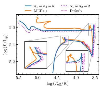
Figure 17: Evolution of a 30 $\mathrm{M}_{\odot}$ star at solar metallicity. The different tracks use the implicit method to enhance energy transport near the Eddington limit (with different choices for $\alpha_{1}$ and $\alpha_{2}$), MLT++, and the MESA default which includes no energy-transport enhancement. Both simulations with the new method use $\Gamma_{\mathrm{c}}=0.5$ and $\delta_{\rm{c}}=10^{-2}$. The MESA default simulation stalls when evolving towards the blue after a RSG phase. Inset plots are made to highlight variations between the runs at TAMS and at the end of the RSG phase.

Figure 16 illustrates the evolution of stars up to 10⁶ $\mathrm{M}_{\odot}$ at high metallicities ($\rm{Z}=0.0142$) using this new approach. The very high mass models are not necessarily meant to represent real stars, but serve as an extreme test of this new approach. In particular, realistic models of supermassive stars need to also take into account general relativistic effects (Chandrasekhar, 1964; Fricke, 1973), which are not included in these simulations. The calculations all used $\Gamma_{\mathrm{c}}=0.5$, $\alpha_{1}=\alpha_{2}=5$ and $\delta_{\rm{c}}=10^{-2}$, which we found to perform consistently across a broad range of masses.

A comparison between the new method, MLT++ and a simulation without any enhancement of energy transport is shown for a 30 $\mathrm{M}_{\odot}$ model in Figure 17. Overall, the new method provides smoother evolution while remaining closer to the result obtained without enhancing energy transport. MLT++ introduces undesirable numerical variations that are particularly visible when the model moves from the blue to the red at TAMS, and when it evolves from the red to the blue after being stripped of most of its H envelope. Lowering $\alpha_{1}$ or $\alpha_{2}$, or increasing $\Gamma_{\mathrm{c}}$ or $\delta_{\rm{c}}$, will produce results closer to those without energy-transport enhancement. Figure 17 also shows two different simulations with the new method using $\alpha_{1}=\alpha_{2}=5$ and $2$. The simulations performed with $\alpha_{1}=\alpha_{2}=2$ take almost triple the number of steps and computation wall time. Selection of these parameters requires balancing performance and similarity to the unenhanced behavior. Users need to carefully assess if such variations have a meaningful impact in their conclusions.

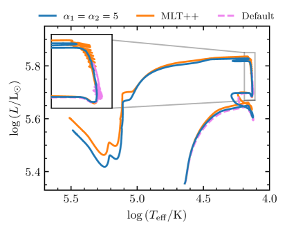
Figure 18: Evolution of a 40 $\mathrm{M}_{\odot}$ star with a 30 $\mathrm{M}_{\odot}$ point mass companion with an initial orbital period of 50 days. Models are computed for solar metallicity and using different methods to enhance energy transport in regions near the Eddington limit.

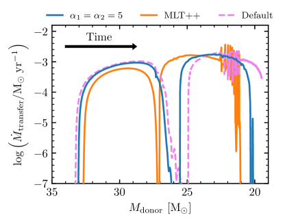
Figure 19: Mass transfer rate $\dot{M}_{\rm{transfer}}$ as a function of donor mass for the binary system shown in Figure 18. All simulations have two significant phases of mass transfer corresponding to interaction during the MS (Case A) and after TAMS (Case AB).

The stability of this implicit method is particularly useful in simulations of binary systems, where small step-to-step variations in $R$ can result in large changes to $\dot{M}$ during Roche lobe overflow. This makes the previous MLT++ method inappropriate.

Figure 18 shows the evolution of a 40 $\mathrm{M}_{\odot}$ model with a 30 $\mathrm{M}_{\odot}$ point mass companion at an initial orbital period of $50$ days. Simulations are performed using no enhancement of energy transfer, MLT++, and the implicit method. In all cases, the models experience an initial mass transfer phase during the MS, and a second mass transfer phase right after TAMS. The simulation without enhanced energy transfer stalls during this second mass transfer phase, exemplifying the computational complexity of modelling stars near the Eddington limit.

Figure 19 demonstrates that although the MLT++ model evolves beyond detachment, large step-to-step variations lead to large changes in mass transfer rates. In contrast, the new implicit method provides a smooth solution throughout the mass transfer phase. An early example of this implicit method enabling the succesful computation of massive binary evolution are the models of $\zeta$ Ophiuchi computed by Renzo & Götberg (2021).

8 Opacity

8.1 Molecular Opacities

Molecules contribute significantly to stellar opacity for $T\lesssim 5000$K (Alexander & Ferguson, 1994; Ferguson et al., 2005). The MESA kap module has been expanded to include low-temperature molecular opacities from Lederer & Aringer (2009) and ÆSOPUS (Marigo & Aringer, 2009). Both opacity sets allow for varying CNO levels. CNO-enhanced molecular opacities find applications in models of red giants, AGB stars, and R Coronae Borealis stars (Schwab, 2019).

Lederer & Aringer (2009) provide Rosseland mean opacity tables for 14 metallicities ranging from Z = $10^{-5}$ to Z = 4$\times$10^-2, and three H mass fractions X = 0.5, 0.7, or 0.8. One can specify seven Z-dependent levels of C-enhancement and three Z-dependent levels of N-enhancement, all with Lodders (2003) solar abundances. The tables span $3.2\leq\log(T/\rm{K})\leq 4.05$ and $-7\leq\log(\rho T_{6}^{-3}/\mathrm{g}\,{\mathrm{c}\mathrm{m}}^{-3})\leq 1$. These opacities are enabled by setting kappa_low_T_prefix = 'kapCN'.

ÆSOPUS (Marigo & Aringer, 2009) allows computation of opacity tables for a variety of solar compositions with the optional inclusion of enhancements (and depletions) to C, N and C/O on top of the basic mixture. We provide a set of ÆSOPUS opacity tables. Additional ÆSOPUS opacity tables can be generated through the ÆSOPUS web-interface, and MESA_DIR/kap/preprocessor/AESOPUS contains information on preparing the tables for MESA.

To compare MESA and the Monash stellar evolution code (Lattanzio, 1986; Frost & Lattanzio, 1996; Karakas & Lattanzio, 2007), custom ÆSOPUS tables were generated with $3.2\leq\log(T/\rm{K})\leq 4.5$ in steps of 0.01 dex and $-7\leq\log(\rho T_{6}^{-3}/\mathrm{g}\,{\mathrm{c}\mathrm{m}}^{-3})\leq 1$ in steps of 0.05 dex. We use steps of 0.5 dex at higher $T$, the Lodders (2003) solar composition, reference metallicities of Z = 0.01 to 0.10 in steps of 0.01 dex and $0.5\leq\rm{X}\leq 0.8$ in steps of 0.1. We set the CNO abundance variation factors fc = $-1$, 0.2, 0.4, 0.6, 1, 1.5, fco = $-1$, $-0.5$, 0, 0.5, 1, 1.5 and fn = 0, 0.4, 0.7, 1.

These tables were installed in MESA and the Monash code. The physics used in the Monash code is reconstructed as closely as possible in MESA (Cinquegrana et al., 2022; Cinquegrana & Joyce, 2022). This includes the basic.net reaction network, treatment of MLT convection (with independently calibrated $\alpha_{\rm MLT}$ parameters of $\alpha_{\rm MLT}$ = 1.931 in MESA, $\alpha_{\rm MLT}$ = 1.86 in Monash), high temperature and molecular opacities (Iglesias & Rogers, 1996; Marigo & Aringer, 2009), an Eddington gray atmosphere, and mass-loss approximations (Reimers, 1975; Blöcker, 1995). We use an $\eta_{\rm Reimers}=0.477$ efficiency factor, and $\eta_{\text{Bl\"{o}cker}}$ = 0.01 in MESA and $\eta_{\text{Bl\"{o}cker}}\,=\,0.02$ in the Monash code (Cinquegrana et al., 2022). Functionality that is not available in both includes the process of defining the border between convective and radiative regions. Here, a relaxation method is used in the Monash code (Lattanzio, 1986), and the predictive mixing algorithm in MESA (MESA IV).

We evolve a $3\,\mathrm{M}_{\odot}$, Z = 0.014 model with MESA and the Monash code. Both models use the same initial conditions and are terminated at the 11th thermal pulse. Figure 20 compares the $L$, $T_{\rm eff}$, and $R$ histories of the two models during the TP-AGB phase. The MESA model reaches higher peak $L$, smaller peak $T_{\rm eff}$, and larger peak $R$ than the Monash model. The differences decrease as the evolution proceeds. Both have very similar interpulse periods, $\simeq$ 7.2$\times$10⁴ yr, after the first few pulses.

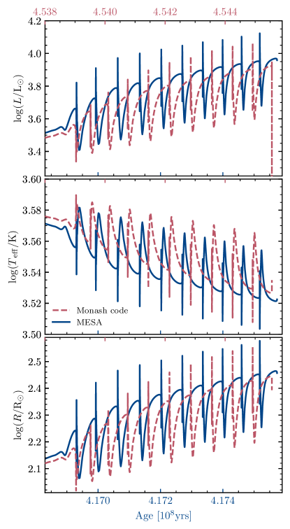
Figure 20: Evolution of $L$, $T_{\rm eff}$ and $R$, respectively, during the TP-AGB phase of 3 $\mathrm{M}_{\odot}$, Z = 0.014 models from MESA (solid) and the Monash code (dashed). The age of the MESA (Monash) stellar model is shown on the bottom (top) x-axis.

8.2 Compton Opacities

At temperatures $\log(T/\rm K)\gtrsim 8.7$, beyond the boundary of the standard opacity tables, the radiative opacity is set by Compton scattering (MESA I, §4.3). Such conditions are often realized in simulations of massive stars and thermonuclear bursts on neutron stars. MESA now calculates the Compton scattering opacity using the prescription of Poutanen (2017), which improves upon the previous approach from Buchler & Yueh (1976). See §4 in Poutanen (2017) for a detailed comparison of the two approaches.

8.3 Conductive Opacities

Energy transport via electron conduction plays an important role, especially in degenerate stellar interiors. The conductive opacities in MESA are expanded versions of the tables from Cassisi et al. (2007), see MESA II, Appendix A.3. Blouin et al. (2020) improved the conductive opacities for H and He in the regime of moderate Coulomb coupling and moderate degeneracy, primarily relevant for the envelopes of DA and DB WDs. We implement their analytical fits for conductive opacities for H and He in MESA.

Figure 21 shows the effect of these new opacities on MESA WD cooling calculations for a $0.9\,\mathrm{M}_{\odot}$ WD with a H atmosphere, confirming the result of Blouin et al. (2020) that the cooling time to reach $T_{\rm eff}=4000\,\mathrm{K}$ can be reduced by $\approx 2\,\rm Gyr$. The difference in cooling times is somewhat smaller for WDs with He atmospheres, as also confirmed in MESA models for AM CVn accretors (Wong & Bildsten, 2021). Salaris et al. (2022) provide a more detailed study of the impact of these updated opacities on WD cooling timescales. The conductive opacities including the Blouin et al. (2020) corrections are now the default in MESA.

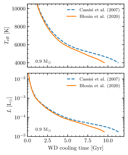
Figure 21: Cooling tracks for $0.9\,\mathrm{M}_{\odot}$ DA WD models using the conductive opacities of Cassisi et al. (2007) and Blouin et al. (2020).

8.4 Radiative Accelerations from the OP Monochromatic Opacities

The radiative acceleration $g_{{\rm rad},i}$ of a given species $i$ represents the acceleration caused by the radiation field. MESA III (§9) describes the inclusion of radiative levitation from Hu et al. (2011), which includes evaluation of the Rosseland mean opacity $\kappa_{\rm R}$ and $g_{{\rm rad},i}$ using the Opacity Project (OP) monochromatic opacity tables (Seaton, 2005). The computation of both of these quantities requires wavelength integrations of monochromatic opacities according to the local mixture, introducing a significant amount of extra time. MESA V (§6.2) briefly describes the steps taken to reduce the time required to evaluate $\kappa_{\rm R}$ and $g_{{\rm rad},i}$. We now describe a new implementation from Mombarg et al. (2022).

The OP tables provide monochromatic cross sections $\sigma_{i}$, equally spaced in

$$v(u)=\frac{15}{4\pi^{4}}\int_{0}^{u}\frac{x^{4}e^{-x}}{(1-e^{-x})^{3}}{\rm d}x,$$ (76)

with a step size $\Delta v$, where 10^-3 $\leq$ $u\,\equiv\,h\nu/k_{\mathrm{B}}T$ $\leq$ 20. The OP tables contain data for H, He, C, N, O, Ne, Na, Mg, Al, Si, S, Ar, Ca, Cr, Mn, Fe, and Ni. The Rosseland mean opacity for cell $k$ is then given by

$$\kappa_{{\rm R},k}=\frac{1}{\mu_{k}}\left(\sum\limits_{n}\frac{1}{\sum\limits_{i}f_{i,k}\sigma_{i}(v_{n})}\Delta v\right)^{-1},$$ (77)

where $\mu_{k}$ is the mean molecular weight and $f_{i}$ the fractional element abundance of species $i$. The monochromatic opacities are sampled at 10,000 points in the frequency parameter $v_{n}$, denoted by index $n$.

In the new implementation, the OP monochromatic data are converted from ($T,n_{e}$) space to ($T,\rho$) space with

$$\log(\rho/{\rm g\ cm}^{-3}) =\log(n_{e}/{\rm cm}^{-3})+\log\mu$$ (78)

$$-\log\Xi-\log(N_{\mathrm{\!A}}/{\rm g}),$$

where $\Xi=\sum\nolimits_{i}f_{i}\Xi_{i}$ is the average number of electrons per atom (given by the OP tables) and $N_{\mathrm{\!A}}$ is Avogadro’s constant. The tables contain data for 3.5 $\leq\log(T/\rm{K})\leq$ 8.0 and $\log(\rho/\mathrm{g}\,{\mathrm{c}\mathrm{m}}^{-3})$ bounds that depend on $\log(T/\rm{K})$. An error is returned for $T$ and $\rho$ beyond these limits.

We select the point in the OP tables with the smallest value of

$$\sqrt{\frac{(\log T_{i}^{\rm OP}-\log T_{k})^{2}}{0.0025}+\frac{(\log\rho_{i}^{\rm OP}-\log\rho_{k})^{2}}{0.25}},$$ (79)

where the different denominators reflect the different OP table spacings.

From this OP data point we select nearest neighbor points and construct a spline interpolant with a maximum degree of three, i.e., a bicubic interpolant. The interpolants are stored such that the opacity can be re-interpolated at the next time step as long as $\log(T/\rm{K})$ has changed by less than twice the grid spacing (0.01 dex), $\log(\rho/\mathrm{g}\,{\mathrm{c}\mathrm{m}}^{-3})$ has changed less than twice its grid spacing (0.1 dex), and the fractional abundances all satisfy

$$\frac{|f_{i,t}-f_{i,t-1}|}{f_{i,t-1}}<\epsilon,$$ (80)

where $t$ and $t-1$ indicate the current and previous time steps, respectively. Empirically, we find for MS models that $\epsilon$ = $10^{-4}$ optimizes the computational efficiency without sacrificing accuracy in $\kappa_{\rm R}$ and $g_{{\rm rad},i}$ (Hui-Bon-Hoa, 2021).

The radiative acceleration of a species is given by

$$g_{{\rm rad},i}=\frac{\mu\kappa_{\rm R}}{\mu_{i}c}\mathcal{F}\gamma_{i},$$ (81)

where $\mu_{i}$ is the molecular weight of the species and $\mathcal{F}$ is the radiative flux. The factor $\gamma_{i}$ is given by

$$\gamma_{i}=\sum\limits_{n}\frac{\sigma_{i}(v_{n})[1-e^{-u(v_{n})}]-a_{i}(v_{n})}{\sum_{j}f_{j}\sigma_{j}(v_{n})}\Delta v,$$ (82)

where the index $j$ runs over all species. The correction terms $a_{i}(v_{n})$ are provided by the OP data. The numerator in Equation (82) is precomputed and stored.

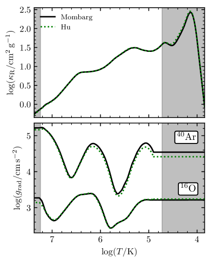
Figure 22: Rosseland mean opacity ($\kappa_{\rm R}$, upper) and the radiative accelerations ($g_{\rm rad}$, lower) of ¹⁶O and ⁴⁰Ar in a 2 $\mathrm{M}_{\odot}$ model with an initial $\rm{Z}$ = 0.02 at a core H mass fraction of $\rm{X}_{\rm c}$ = 0.2. Green dotted curves show the MESA III (Hu) treatment, and black solid curves show the current treatment (Mombarg). Shaded areas indicate convective regions.

In the new implementation, optimized for models with a convective core and radiative envelope, the envelope is divided into two equal regions based on the number of cells (regardless of the outer convection cells). For each region, the $\gamma_{i}$ factors are pre-computed using an average mixture of the region

$$\left<f_{i}\right>=\left(\sum\limits_{k=k_{1}}^{k_{2}}f_{i,k}\right)\left(\sum\limits_{i}\sum\limits_{k=k_{1}}^{k_{2}}f_{i,k}\right)^{-1},$$ (83)

where $k_{1}$ and $k_{2}$ are the first and last cell index of a region. Near the boundary of these two regions, 15 cells on each side, the value of $\log g_{{\rm rad},i}$ is blended

$$\log g_{{\rm rad},i}=\alpha_{i}\log g_{{\rm rad},i,1}+(1-\alpha_{i})\log g_{{\rm rad},i,2},$$ (84)

where $\log g_{{\rm rad},i,1}$ is computed using the average mixture $\left<f_{i,1}\right>$ of the first region, and $\log g_{{\rm rad},i,2}$ from the average mixture of the second region. The parameter $\alpha_{i}$ varies linearly between 0 and 1 as a function of cell number in the region where blending takes place.

Figure 22 compares $\kappa_{\rm R}$ and $g_{{\rm rad},i}$ from MESA III and the present method. The cell-averaged difference and maximum difference ($|\log g_{\rm rad}^{\rm Hu}-\log g_{\rm rad}^{\rm Mombarg}|/\log g_{\rm rad}^{\rm Hu}$) for ¹⁶O are 0.007 and 0.042, respectively, and for ⁴⁰Ar are 0.02 and 0.03, respectively. The differences in $g_{{\rm rad}}$ for ¹⁶O are typical for most isotopes. The new implementation is about 5 times faster for MS stars.

Enabling this capability requires a data file containing the manipulated OP monochromatic data, doi:https://doi.org/10.5281/zenodo.6858178 (catalog https://doi.org/10.5281/zenodo.6761478).

9 Diffusion Coefficients

MESA III and MESA IV describe the implementation of element diffusion in MESA using the Burgers (1969) equations with diffusion coefficients based on Paquette et al. (1986), and updated with the coefficients of Stanton & Murillo (2016). For strong plasma coupling in the liquid regime (where the multi-component plasma coupling parameter $\Gamma_{\rm MCP}\equiv q_{e}^{2}\langle Z^{5/3}\rangle/a_{e}k_{\rm B}T\gtrsim 1$), these coefficients disagree by a factor of a few with more accurate molecular dynamics (MD) methods (MESA III, Bauer et al. 2020, Caplan et al. 2022).

Until recently, it was unclear how to generalize these results to the arbitrary plasma mixtures needed for stellar models. However, Caplan et al. (2022) show that in the liquid regime ($10\lesssim\Gamma_{\rm MCP}\lesssim 200$), diffusion coefficients are approximated to within $\sim 10$% accuracy by using a fit to an equivalent one-component plasma (OCP) coefficient calculated with MD, and then scaling with charge as

$$D_{j}=\left(\frac{Z_{j}}{\langle Z\rangle}\right)^{-0.6}D_{\rm OCP}~{},$$ (85)

where $D_{j}$ is the diffusion coefficient of species $j$, $Z_{j}$ is the charge of species $j$, $\langle Z\rangle\equiv\sum_{j}n_{j}Z_{j}/n_{\rm ions}$ is the average charge of ions in the liquid, and $D_{\rm OCP}$ is the diffusion coefficient for an equivalent OCP with coupling and screening set by the mixture averages. This scaling is justified by the fact that in the liquid regime, ion diffusion can be described in terms of spheres experiencing Stokes-Einstein drift through a viscous liquid (Bildsten & Hall, 2001; Daligault, 2006), with the effective radii of different ions set by their charge relative to the background plasma (Bauer et al., 2020; Caplan et al., 2022). The $D_{\rm OCP}$ term therefore captures the physics of the global viscosity experienced by all ions, while the scaling with charge captures the different effective radii of ions experiencing Coulomb interactions with the background plasma.

Since the diffusion solver in MESA is cast in terms of the Burgers (1969) equations, coefficients must be recast in terms of the binary resistance coefficients $K_{ij}$ between species $i$ and $j$ rather than the net diffusion coefficients $D_{j}$. At strong plasma coupling ($\Gamma_{\rm MCP}\gtrsim 10$), these coefficients must satisfy the relation

$$D_{j}=\frac{n_{j}k_{\rm B}T}{\sum_{i}K_{ij}}~{}.$$ (86)

The resistance coefficients $K_{ij}$ must also be symmetric ($K_{ij}=K_{ji}$), motivating

$$K_{ij}=\frac{n_{i}n_{j}(Z_{i}Z_{j})^{0.6}k_{\rm B}T}{n_{\rm ions}\langle Z^{0.6}\rangle\langle Z\rangle^{0.6}D_{\rm OCP}}~{},$$ (87)

where $\langle Z^{0.6}\rangle\equiv\sum_{j}n_{j}Z_{j}^{0.6}/n_{\rm ions}$. The resistance coefficients of Equation (87) reduce to the desired net diffusion coefficients of Equation (85) under the summation required in Equation (86).

We calculate the OCP diffusion coefficient $D_{\rm OCP}$ using the Caplan et al. (2022) fit to high-resolution MD, which is given in terms of $\Gamma_{\rm MCP}$ and electron screening length $\lambda_{e}$. To calculate the value of $\lambda_{e}$ as input for the diffusion coefficients, we follow the method described in MESA IV based on Stanton & Murillo (2016) for non-relativistic electrons at $\rho<10^{6}\,\rm g\,cm^{-3}$. Electrons become relativistic at higher densities, and we therefore switch to the relativistic screening length $\lambda_{e}=\left(2k_{\rm F}\sqrt{\alpha/\pi}\right)^{-1}$ for densities $\rho>10^{6}\,\rm g\,cm^{-3}$, where $\alpha$ is the fine-structure constant and $k_{\rm F}=(3\pi^{2}n_{e})^{1/3}$.

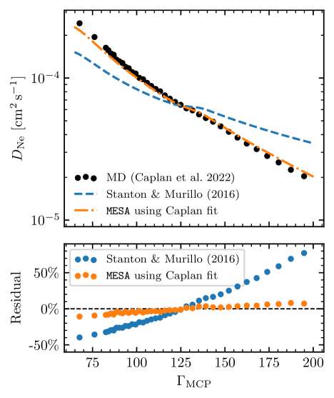
Figure 23: Diffusion coefficient of ²²Ne in the liquid interior profile of a cooling C/O WD model. The residuals in the lower panel are relative to the Caplan et al. (2022) MD for a C/O/Ne plasma mixture shown in the top panel.

Figure 23 shows the ²²Ne diffusion coefficient in a MESA model of a $0.6\,\mathrm{M}_{\odot}$ C/O WD, which has historically been a key source of uncertainty in the rate at which ²²Ne settles toward the center of the WD (Bildsten & Hall, 2001; Deloye & Bildsten, 2002; García-Berro et al., 2008). Such C/O mixtures with trace ²²Ne are in the liquid phase for $\Gamma_{\rm MCP}\lesssim 200$ (Caplan et al., 2020; Blouin & Daligault, 2021), though distillation of ²²Ne may also occur for sufficient ²²Ne concentration (Blouin et al., 2021).

Figure 23 also shows the MD coefficients from Caplan et al. (2022) (these closely match the MD coefficients of Hughto et al. 2010) along with diffusion coefficients obtained from Equations (86) and (87) for MESA profiles of our C/O WD model with a similar interior composition. The coefficients based on Stanton & Murillo (2016) vary from the MD results by a factor of two or more, while the residuals for our implementation of the Caplan et al. (2022) coefficients are 10% or less. This represents an order of magnitude improvement on the uncertainties for diffusion coefficients in the strongly coupled regime relative to the previous MESA implementation, while also providing a procedure that is generalizable to compositions other than just C/O/Ne mixtures (Equation 87).

We have implemented these Caplan et al. (2022) diffusion coefficients as the default coefficients in MESA for $\Gamma_{\rm MCP}>10$, with a smooth transition from the Stanton & Murillo (2016) coefficients over the range $3<\Gamma_{\rm MCP}<10$. The diffusion coefficients in the liquid WD regime are now accurate to $\approx 10\%$ for $10\lesssim\Gamma_{\rm MCP}\lesssim 200$, a substantial improvement compared to our previous methods.

When crystallization occurs for $\Gamma_{\rm MCP}\gtrsim 200$, we assume that freezing into the solid phase causes the diffusion coefficient to go to zero. We implement this with a smooth turnoff near the crystallization boundary using the smoothed phase parameter $\phi$ from Skye (§4.1), so that the diffusion velocities are zero for $\phi\geq 0.5$.

10 Nuclear physics

MESA models calculate the energy generation rates and composition changes due to nuclear burning over a large range of $T$, $\rho$, and $X_{i}$. The nuclear evolution of the chemical composition dominates the total cost of a model (memory + CPU) when the number of isotopes is $\gtrsim$ 30. Here we report progress on nuclear reaction rates, a new operator split burning option, and enhanced reaction rate outputs.

10.1 Reaction rates updates

MESA’s default reaction rate for $\mathrm{{}^{7}Be}(e^{-},\nu_{e})\mathrm{{}^{7}Li}$ came from REACLIB (Cyburt et al., 2010). However, REACLIB is only defined for $T>10^{7}$ K, and assumes that all atoms are ionized. While this is a reasonable assumption for reactions that occur deep in the stellar interior, significant Li production can occur in stellar envelopes with $T<10^{7}$ K where the reaction rate then depends on the ionization balance (Schwab, 2020). The new default (as of r22.05.1) for this rate is Simonucci et al. (2013) which incorporates ionization contributions.

REACLIB defines a reverse reaction as the endothermic direction. However, this direction depends on the nuclear masses assumed during the evaluation. For consistency with the nuclear masses used in MESA, we define the reverse rate based on the nuclear masses from masslib_library_5.data. This affects reactions with uncertain nuclear masses; for instance, the reaction $\mathrm{{}^{55}Cu}\left(\gamma,p\right)\mathrm{{}^{54}Ni}$ has a $Q=0.293\,\mathrm{M}\mathrm{eV}$ (exothermic) from “rpsm” (Rauscher 1999, priv. comm) and a $Q=-0.07256\,\mathrm{M}\mathrm{eV}$ (endothermic) from “ths8”  (Cyburt et al., 2010). Incorrectly determining which reaction is endothermic leads to large errors when the reverse rate is computed from detailed balance.

10.2 Operator split nuclear burning

By default MESA uses a nuclear reaction network that is fully coupled to the stellar hydrodynamics (MESA I), solving for the changes in the composition simultaneously with the changes in stellar structure quantities. This approach provides consistency between the nuclear physics and stellar hydrodynamics, but can place limits on the maximum time step. When $T\gtrsim 3\times 10^{9}$ K, the time step is limited by the nuclear burning timescale, and the composition enters a dynamic equilibrium state where large forward and reverse reaction rates nearly cancel each other, potentially leading to numerical errors when subtracting large values from one another (MESA III). During the final stages of evolution to core-collapse, time steps of $\delta t<10^{-10}$ s are common (Farmer et al., 2016). This can make evolution to core collapse a resource-consuming endeavor.

MESA has the capability to perform an operator-split procedure (op_split_burn) to compute the composition change and energy generation. Cells with high $T$ use operator splitting. For each such cell, MESA computes the change in composition over the timestep $\delta t$ with a semi-implicit midpoint rule (Bader & Deuflhard, 1983). An operator-split cell can then take multiple sub-steps, allowing the composition to evolve at fixed $T$ and $\rho$ with an adaptive time step. The nuclear energy generated $\epsilon_{\mathrm{nuc}}$ is calculated by taking the difference between the starting and final compositions, and energy loss due to neutrinos from nuclear reactions $\epsilon_{\mathrm{\nu}}$ is accounted for.

This scheme allows accurate tracking of the net nuclear energy generation rate and composition changes. However, operator-split burning cannot calculate the partial derivatives of these terms with respect to $T$ or $\rho$ for the matrix solver. These partial derivative matrix terms are thus set to zero. This removes the difficulty of the partial derivatives varying in sign and magnitude over short timescales, and enables the solver to more robustly find a solution within the requested tolerances.

Figure 24 compares the fully-coupled (unsplit) and operator split solutions in the central $T$-$\rho$ plane for a 30 $\mathrm{M}_{\odot}$, solar-metallicity model evolved from the ZAMS to the formation of the iron core. We enable op_split_burn for any cell with a $T>10^{9}$ K. The evolutions are nearly identical up to $T_{c}\approx 3\times 10^{9}$ K, after which the fully-coupled solution evolves to a slightly larger $\rho$. These differences are comparable to variations arising from other physics choices, such as the nuclear reaction rate screening prescription (see Appendix A.2 of MESA V). Evolution up to the formation of the iron core took approximately equal number of timesteps. Evolving the models further to the onset of core-collapse with “gold” tolerances (MESA V), the operator split model only required an additional $\approx$ 200 time steps, while the fully-coupled model failed to reach the onset of core-collapse after an additional $\approx$ 140,000 time steps.

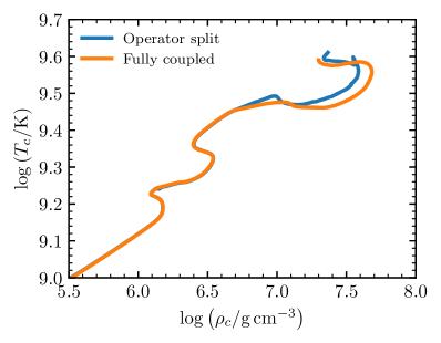
Figure 24: Central $T$-$\rho$ tracks of a 30 $\mathrm{M}_{\odot}$ star evolved from ZAMS to formation of the iron core.

Operator splitting can provide a significant speedup during Si and Fe burning by reducing the number of time steps needed, and may be the only way to make certain problems tractable. It is however less efficient than a fully-coupled model during earlier stages of evolution due to the additional sub-steps taken by each operator-split cell. Thus, we suggest considering operator splitting only for models evolving beyond core C-depletion. It is difficult to say which treatment is more accurate; fully-coupled calculations include more physics but can be subject to numerical errors, while our operator-split calculations ignore the physics in the partial derivatives, but provide a more numerically stable solution.

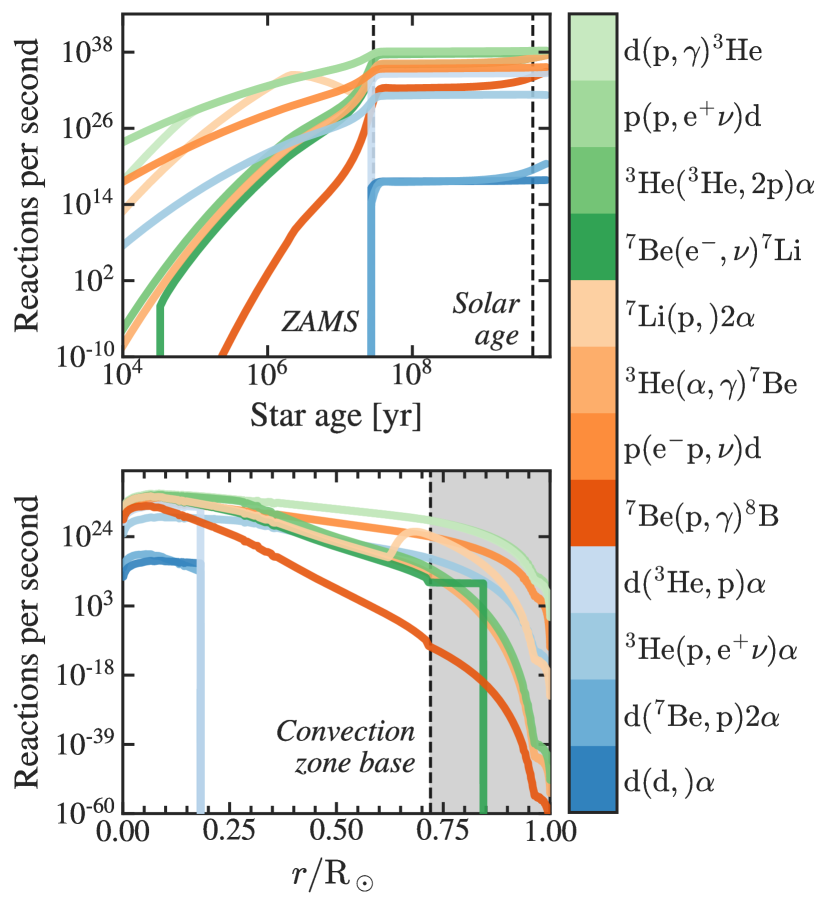
Figure 25: Nuclear reactions rates ongoing in the Sun. Upper: Evolution of reaction rates from the pre-main sequence to core H exhaustion. Lower: Profiles at the current solar age as a function of the distance from the solar center. The reactions in the colorbar are ordered from top to bottom according to their frequency.

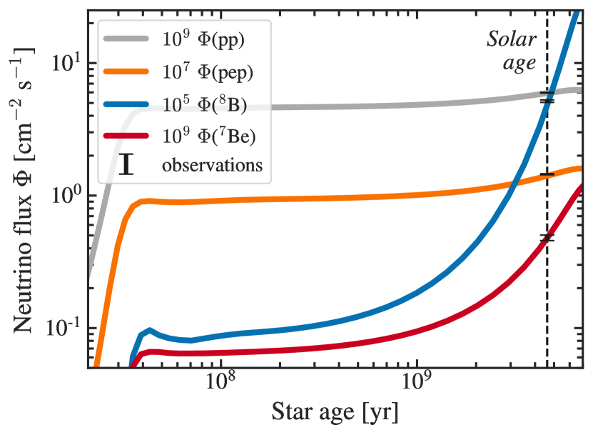
Figure 26: The evolution of solar electron neutrino flux at Earth. The predicted values for the present Sun are in satisfactory agreement with the observed values after correction for flavor effects: $\Phi(\rm{pp})/10^{9}=$ 5.934 (MESA), 5.971 $\pm$ 0.035 (Borexino); $\Phi(\rm{pep})/10^{7}=$ 1.408 (MESA), 1.448 $\pm$ 0.013 (Borexino); $\Phi(^{7}\rm{Be})/10^{9}=$ 0.476 (MESA), 0.480 $\pm$ 0.023 (Borexino); and $\Phi(^{8}\rm{B})/10^{5}=$ 4.780 (MESA), 5.160 $\pm$ 0.110 (Borexino) cm^-2 s^-1.

10.3 Reaction rate output

MESA has the new capability to output individual nuclear reaction rates and related quantities to the history or profile data files. Using ${\tt add\_raw\_rates}$ will output the rates of all reactions. Alternatively, ${\tt raw\_rate}$ with the name of a specific reaction will report only that reaction. Similarly, ${\tt add\_eps\_neu\_rates}$, ${\tt add\_eps\_nuc\_rates}$, and ${\tt add\_screened\_rates}$ provide neutrino energy rates, nuclear energy rates, and screened reaction rates.

As an example, Figure 25 shows the total reaction rates of a $1\,\mathrm{M}_{\odot}$ model evolved to the solar age, and the profiles of the reaction rates at the solar age. Figure 26 further shows the evolution of the solar electron neutrino fluxes and a comparison with the observed solar electron neutrino fluxes (see also Farag et al., 2020) after correction for flavor mixing (Bergström et al., 2016). The model agreement with measurements is similar to that obtained using the ASTEC stellar evolution code (Bellinger & Christensen-Dalsgaard, 2022).

11 Constants

The MESA const module provides mathematical, physical, and astronomical constants relevant to stellar astrophysics (MESA I, Section 4.1). The values in this module have been updated to reflect new definitions and conventions. Some microphysics inputs (e.g., opacity, EOS, reaction rates) use slightly different constants in constructing their tables or expressions. Such cases are usually beyond our control, and the updates in this section do not apply to those instances.

As part of the revision of the SI, the values of the physical constants $e$, $h$, $k_{\mathrm{B}}$, and $N_{\mathrm{\!A}}$ are now exact (Newell et al., 2018). We have adopted these values and ensured that other constants composed of these and other exact values (e.g., the Stefan-Boltzmann constant) are defined in a consistent manner. For other physical constants, (e.g., $G$) we use CODATA 2018 (Tiesinga et al., 2021).

MESA follows IAU recommendations for astronomical constants, currently adopting nominal solar and planetary quantities from IAU 2015 Resolution B3 (Mamajek et al., 2015). We follow the recommended procedure of deriving nominal solar and planetary masses from the mass parameters $(GM)$ and the adopted value of $G$. We also adopt the convention that the nominal radii of planetary bodies are the equatorial radii.

12 Infrastructure

12.1 Migration to GitHub

MESA development began in 2007 with a Subversion (SVN) repository hosted on SourceForge, and from 2017$-$2020 this SVN repository was hosted by Assembla. Beginning in December 2020, development shifted to GitHub, with the root of the new Git repository corresponding to SVN r15140. An archival copy of the SVN development history is available at doi:https://doi.org/10.5281/zenodo.4745225 (catalog 10.5281/zenodo.4745225). The shift to GitHub paves the way for a new era of collaborative MESA development and expanded interaction with the astrophysics community.

As Git repositories can have a non-linear commit history, we will no longer denote public releases with a revision number. In SVN, this counted the number of commits from the beginning of MESA’s development. Instead, public releases will now be identified by the date, in the format YY.MM.I, where YY is the final two-digits of the year, MM is the two digit month number, and I is a version (usually 1) to distinguish multiple releases in a given month. While we do not recommend publishing an article based on non-released versions of MESA, if necessary we suggest using the first 7 characters of the Git commit hash as the version number.

12.2 MESA TestHub

With the transition from SVN to Git, the versioning and branching scheme used in the development of MESA changed substantially. A major overhaul of the collection and distribution of continuous integration test results on TestHub (https://testhub.mesastar.org) was necessary. We now highlight these and other changes made since MESA V.

With Git, understanding the relationship of a commit to other commits requires knowledge of the commit graph. To dynamically obtain and update this information, TestHub uses GitHub webhooks and APIs. Upon pushing to the GitHub remote, GitHub now sends a request to TestHub to update its internal tree of commits. This is done by querying the GitHub API for a current list of branches and the head commits of each. TestHub removes any references to branches that are no longer in GitHub and updates the branches table in the TestHub database, adding commits as needed even if they have not had any tests conducted. This allows easy identification of commits that have not yet been tested. We also now store data about commits, such as the authors, commit messages, and commit times directly in the TestHub database for more convenient access.

To view the detailed changes made in a given commit, each commit-specific page on TestHub links to the appropriate page on GitHub. Additionally, most views in TestHub now have a branch selector dropdown so developers can look at commits on a specific branch, and we rely on the GitHub API to order these commits within a branch.

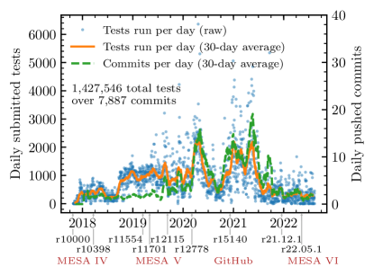
Figure 27: Daily tests submitted since the instantiation of TestHub, spanning the SVN and Git eras. To smooth over the day-to-day variability, we also show 30-day rolling averages of submitted tests and pushed commits. Below the x-axis are dates of public releases and other milestones such as instrument papers and the SVN-to-Git transition.

Figure 27 shows the total number of individual test instances (i.e., results for a single test case from a single computer) and daily commits submitted since the launch of TestHub in late 2017. Unsurprisingly, the rate of test submissions is strongly correlated with the rate of commits. Substantial deviations occur due to different testing computers coming on- and offline, and because some commits focus on documentation and do not trigger testing runs on automated testing setups. Figure 27 also shows the dates of public releases and key milestones. The switch from SVN to Git was shortly after release r15140, and there is a smooth transition between the eras.

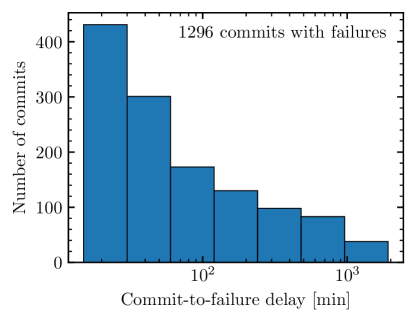
Figure 28: Distribution of delay times from when a commit is pushed to when a failure is first reported.

The MESA test suite takes $\sim$ 100 core hours to complete when run on a modern workstation. To reduce this runtime while still providing diagnostic information, many tests have optional steps that can be skipped, with the next inlist loading a saved model. The total time for a test suite run is roughly halved when these parts are skipped. Skipping optional inlists has drawbacks in requiring saved models, which can generate spurious failures when skipping inlists. At least one computer runs all inlists on all tests on the main branch.

We now assess how quickly our distributed and automated continuous integration workflow can identify a failure. Figure 28 shows that most failures are detected within an hour of the commit, and more than a third are detected within thirty minutes. This prompt turnaround comes from computing clusters configured to check for new commits every few minutes, and then launch a full test suite run upon detecting a new commit. Some clusters are configured to detect and test commits on any branch of the MESA GitHub repository, allowing full testing coverage during feature development and ensuring that new features pass the test suite before being merged into the main branch.

Awareness of test failure and the commit responsible is useful, but having the detailed output of a failing test is often essential in quickly identifying and rectifying the regression. TestHub now collects information on the runtime, computer architecture, broad failure type (such as a compilation error or a runtime error), and the stdout and stderr logs of the compilation and/or test case in the event of a failure. When present, these logs are accessible by links next to the failure indicator. This allows developers to quickly identify what led to the unexpected behavior without having to request more data from the owner of the computer that submitted it. These updates to TestHub improve the pace, efficiency, and quality of MESA source code development.

12.3 User Contributions

MESA has a Zenodo community to encourage users to publicly archive their input and output files. To make user-contributed routines easier to share while minimizing maintenance, we have additionally created the mesa-contrib repository.

Routines in mesa-contrib can be implemented via MESA’s hooks with a few Fortran include statements. If the build environment defines the location of mesa-contrib, then it is included by default as a search path when MESA is compiled. Currently, mesa-contrib contains routines for the atmospheric $T(\tau)$ relations and corresponding MLT parameters implemented by Mosumgaard et al. (2018b) and for angular momentum transport by the enhanced Tayler–Spruit dynamo described by Fuller et al. (2019). To ease the burden of maintenance, mesa-contrib is only intended to work with the latest public MESA release.

12.4 NuDocker

Reproducibility is a goal of open science and a tenet of scientific research. Provenance, as the term relates to software instruments (Van den Bussche & Vianu, 2001; Carata et al., 2014; Stodden et al., 2018), is the ability to record the full history of a result. Scientific research is generally held to be of good provenance when previous results, perhaps decades old, can be reproduced. The aim is to preserve the final knowledge object and the capability to perform the scientific actions that are the foundation of the knowledge object. Thus, we seek to preserve not only the numerical calculation, but accelerate future research by archiving the computational environment.

Provenance enables reproducing past simulations and performing new calculations with different physics or numerical options. A challenge is that compilers change, linked libraries evolve, and operating systems progress. Many science results have been obtained with older versions of MESA, which in most cases are not obsolete and therefore remain valuable. NuDocker^, provides a solution to the provenance challenge by being able to run older versions of MESA with age-appropriate compilers, libraries, and operating system using light-weight, OS-level virtualization (e.g., Docker). NuDocker provides four Docker images that can be launched with one terminal command, and has been tested and used in 14 out-of-the-box MESA versions from r4942 to r22.05.1. A hallmark of Docker virtualization is the minimal performance penalty compared to running natively (Felter et al., 2014, 2015).

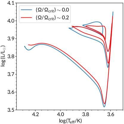
Figure 29: Reproduction of Figure 13 from Farmer et al. (2015) using release r6794 in NuDocker: HRD of two 8 $\mathrm{M}_{\odot}$ models; one non-rotating (blue) and one rotating at $\Omega/\Omega_{\rm crit}$ $\sim$ 0.2 (red). The evolutions span from H depletion to He depletion.

As an example of the ability to provide almost decade-old results with NuDocker, Figure 29 reproduces Figure 13 from Farmer et al. (2015) using the same MESA version 6794 from July 2014 and inlists as in Farmer et al. (2015). The virtual containers allow older versions of MESA to be run with bit-for-bit consistency for all versions after 7503 (see MESA III), thereby enabling older versions of MESA to be run on modern hardware, and preserving the required system environment to enable new research.

13 Summary

We explain significant new capabilities and improvements implemented in MESA since the publication of MESA I through MESA V. Advances in automatic differentiation (§2) and time-dependent convection (§3) will open opportunities for future investigations in stellar evolution. Discussion of the current treatment of the energy equation (§5), stellar atmospheres (§6), and new formalisms for treating starspots and superadiabatic convection (§7) will enhance the study of stellar physics. Upgrades to the equation of state (§4), opacity (§8), element diffusion coefficients (§9), nuclear reaction rates (§10), and physical constants (§11) will increase the robustness of stellar evolution models. The transition to GitHub, upgrades to the MESA TestHub continuous integration framework (§12), the opening of a mesa-contrib repository, and NuDocker’s ability to run older versions of MESA will lead to an efficient and distributed model of source code development. Inlists and related materials for all the figures are available at doi:https://doi.org/10.5281/zenodo.6968760 (catalog 10.5281/zenodo.6968760).

We thank Dr. Bill Paxton for two decades of his amazing talents, extraordinary energy, and his generous gift of MESA to the astronomy and astrophysics community.

We also thank Amy Mainzer for Figure 4 of MESA III making an appearance in the movie Don’t Look Up (first noted by Jared Goldberg), and the participants of the MESA Summer Schools for their willingness to experiment with new capabilities and modalities of delivery. We thank the anonymous referee for a constructive, detailed, and thoughtful report that improved our manuscript. Finally, we thank Susie Groves for her heroic assistance in enabling the completion of this MESA VI instrument paper under challenging circumstances.

The MESA Project is supported by the National Science Foundation (NSF) under the Software Infrastructure for Sustained Innovation program grants ACI-1663684, ACI-1663688, and ACI-1663696. This research was supported in part by the NSF under Grant No. NSF PHY-1748958 for the Kavli Institute for Theoretical Physics. W.H.B acknowledges support from the UK Science and Technology Facilities Council (STFC) through grant ST/R0023297/1. G.C.C acknowledges support by the Australian Research Council Centre of Excellence for All Sky Astrophysics in 3 Dimensions (ASTRO 3D), through project number CE170100013 and the Astronomical Society of Australia. R.F acknowledges support of the University of Amsterdam’s Helios cluster which was supported by a European Research Council grant 715063, (PI S.E. de Mink) F.H acknowledges funding through an NSERC Discovery Grant, through NSERC project award SAPPJ-2021-00032 and through the NSF under Grant PHY-1430152 for the JINA Center for the Evolution of the Elements. The Flatiron Institute is supported by the Simons Foundation. A.S.J thanks the Gordon and Betty Moore Foundation (Grant GBMF7392) and the National Science Foundation (Grant No. NSF PHY-1748958) for supporting this work. M.J acknowledges the Lasker Data Science Fellowship awarded by the Space Telescope Science Institute, and thanks Marc Pinnsoneault, Jen van Saders, and Jamie Tayar for many hours of consultation on the Yale Rotating Stellar Evolution Code and its documentation. J.S acknowledges support by NASA through Hubble Fellowship grant # HST-HF2-51382.001-A awarded by the Space Telescope Science Institute, which is operated by the Association of Universities for Research in Astronomy, Inc., for NASA, under contract NAS5-26555, by the A.F. Morrison Fellowship in Lick Observatory, and by the National Science Foundation through grant ACI-1663688. R.S acknowledges support by the National Science Center, Poland, Sonata BIS project 2018/30/E/ST9/00598. A.T is a Research Associate at the Belgian Scientific Research Fund (F.R.S.-F.N.R.S.). F.X.T acknowledges support by NASA under the Astrophysics Theory Program grant NNH21ZDA001N-ATP, and by the NSF under Grant PHY-1430152 for the JINA Center for the Evolution of the Elements. T.L.S.W thanks support by the Gordon and Betty Moore Foundation through Grant GBMF5076. J.S.G.M acknowledges support by the KU Leuven Research Counsil (grant C16/18/005: PARADISE). O.T was supported by a FONDECYT project 321038. P.M. acknowledges support from the FWO junior postdoctoral fellowship No. 12ZY520N. This research made extensive use of the SAO/NASA Astrophysics Data System (ADS).

References

- Abbott et al. (2018) Abbott, B. P., Abbott, R., Abbott, T. D., et al. 2018, Living Reviews in Relativity, 21, 3, doi: 10.1007/s41114-018-0012-9
- Abdurro’uf et al. (2022) Abdurro’uf, Accetta, K., Aerts, C., et al. 2022, ApJS, 259, 35, doi: 10.3847/1538-4365/ac4414
- Abe et al. (2016) Abe, K., Haga, Y., Hayato, Y., et al. 2016, Astroparticle Physics, 81, 39, doi: 10.1016/j.astropartphys.2016.04.003
- Acciarri et al. (2016) Acciarri, R., Acero, M. A., Adamowski, M., et al. 2016, arXiv e-prints, arXiv:1601.02984. https://arxiv.org/abs/1601.02984
- Acernese et al. (2015) Acernese, F., Agathos, M., Agatsuma, K., et al. 2015, Classical and Quantum Gravity, 32, 024001, doi: 10.1088/0264-9381/32/2/024001
- Akeson et al. (2019) Akeson, R., Armus, L., Bachelet, E., et al. 2019, arXiv e-prints, arXiv:1902.05569. https://arxiv.org/abs/1902.05569
- Akutsu et al. (2021) Akutsu, T., Ando, M., Arai, K., et al. 2021, Progress of Theoretical and Experimental Physics, 2021, 05A102, doi: 10.1093/ptep/ptab018
- Al Kharusi et al. (2021) Al Kharusi, S., BenZvi, S. Y., Bobowski, J. S., et al. 2021, New Journal of Physics, 23, 031201, doi: 10.1088/1367-2630/abde33
- Alexander & Ferguson (1994) Alexander, D., & Ferguson, J. 1994, The Astrophysical Journal, 437, 879
- Almgren et al. (2020) Almgren, A., Sazo, M., Bell, J., et al. 2020, The Journal of Open Source Software, 5, 2513, doi: 10.21105/joss.02513
- Andreoni et al. (2022) Andreoni, I., Coughlin, M. W., Almualla, M., et al. 2022, ApJS, 258, 5, doi: 10.3847/1538-4365/ac3bae
- Andringa et al. (2016) Andringa, S., et al. 2016, Adv. High Energy Phys., 2016, 6194250, doi: 10.1155/2016/6194250
- Araki et al. (2005) Araki, T., et al. 2005, Phys. Rev. Lett., 94, 081801, doi: 10.1103/PhysRevLett.94.081801
- Artigau et al. (2014) Artigau, É., Sivaramakrishnan, A., Greenbaum, A. Z., et al. 2014, in Society of Photo-Optical Instrumentation Engineers (SPIE) Conference Series, Vol. 9143, Space Telescopes and Instrumentation 2014: Optical, Infrared, and Millimeter Wave, 914340, doi: 10.1117/12.2055191
- Ashok & Banerjee (2003) Ashok, N. M., & Banerjee, D. P. K. 2003, A&A, 409, 1007, doi: 10.1051/0004-6361:20031160
- Astropy Collaboration et al. (2018) Astropy Collaboration, Price-Whelan, A. M., Sipőcz, B. M., et al. 2018, AJ, 156, 123, doi: 10.3847/1538-3881/aabc4f
- Astropy Collaboration et al. (2022) Astropy Collaboration, Price-Whelan, A. M., Lian Lim, P., et al. 2022, arXiv e-prints, arXiv:2206.14220. https://arxiv.org/abs/2206.14220
- Baalrud & Daligault (2014) Baalrud, S. D., & Daligault, J. 2014, Physics of Plasmas, 21, 055707, doi: 10.1063/1.4875282
- Bader & Deuflhard (1983) Bader, G., & Deuflhard, P. 1983, Numerische Mathematik, 41, 373, doi: 10.1007/BF01418331
- Baiko (2019) Baiko, D. A. 2019, MNRAS, 488, 5042, doi: 10.1093/mnras/stz2041
- Baiko & Chugunov (2022) Baiko, D. A., & Chugunov, A. I. 2022, MNRAS, 510, 2628, doi: 10.1093/mnras/stab3613
- Baiko et al. (2001) Baiko, D. A., Potekhin, A. Y., & Yakovlev, D. G. 2001, Phys. Rev. E, 64, 057402, doi: 10.1103/PhysRevE.64.057402
- Ball (2021) Ball, W. H. 2021, Research Notes of the American Astronomical Society, 5, 7
- Ball et al. (2018) Ball, W. H., Chaplin, W. J., Schofield, M., et al. 2018, The Astrophysical Journal Supplement Series, 239, 34, doi: 10.3847/1538-4365/aaedbc
- Barnes et al. (2021) Barnes, J., Zhu, Y. L., Lund, K. A., et al. 2021, ApJ, 918, 44, doi: 10.3847/1538-4357/ac0aec
- Bartholomew-Biggs et al. (2000) Bartholomew-Biggs, M., Brown, S., Christianson, B., & Dixon, L. 2000, Journal of Computational and Applied Mathematics, 124, 171, doi: 10.1016/S0377-0427(00)00422-2
- Baturin et al. (2019) Baturin, V. A., Däppen, W., Oreshina, A. V., Ayukov, S. V., & Gorshkov, A. B. 2019, A&A, 626, A108, doi: 10.1051/0004-6361/201935669
- Bauer et al. (2017) Bauer, E. B., Schwab, J., & Bildsten, L. 2017, ApJ, 845, 97, doi: 10.3847/1538-4357/aa7ffa
- Bauer et al. (2020) Bauer, E. B., Schwab, J., Bildsten, L., & Cheng, S. 2020, ApJ, 902, 93, doi: 10.3847/1538-4357/abb5a5
- Beacom & Vogel (1999) Beacom, J. F., & Vogel, P. 1999, Phys. Rev. D, 60, 033007, doi: 10.1103/PhysRevD.60.033007
- Beichman et al. (2012) Beichman, C. A., Rieke, M., Eisenstein, D., et al. 2012, in Society of Photo-Optical Instrumentation Engineers (SPIE) Conference Series, Vol. 8442, Space Telescopes and Instrumentation 2012: Optical, Infrared, and Millimeter Wave, 84422N, doi: 10.1117/12.925447
- Bellinger & Christensen-Dalsgaard (2022) Bellinger, E. P., & Christensen-Dalsgaard, J. 2022, MNRAS, arXiv:2206.13570. https://arxiv.org/abs/2206.13570
- Bellm et al. (2022) Bellm, E. C., Burke, C. J., Coughlin, M. W., et al. 2022, ApJS, 258, 13, doi: 10.3847/1538-4365/ac4602
- Bellm et al. (2019) Bellm, E. C., Kulkarni, S. R., Graham, M. J., et al. 2019, PASP, 131, 018002, doi: 10.1088/1538-3873/aaecbe
- Bergström et al. (2016) Bergström, J., Gonzalez-Garcia, M. C., Maltoni, M., et al. 2016, Journal of High Energy Physics, 2016, 132, doi: 10.1007/JHEP03(2016)132
- Bianco et al. (2022) Bianco, F. B., Ivezić, Ž., Jones, R. L., et al. 2022, ApJS, 258, 1, doi: 10.3847/1538-4365/ac3e72
- Biermann (1932) Biermann, L. 1932, ZAp, 5, 117
- Bildsten & Hall (2001) Bildsten, L., & Hall, D. M. 2001, ApJ, 549, L219, doi: 10.1086/319169
- Blöcker (1995) Blöcker, T. 1995, A&AS, 297, 727
- Blouin & Daligault (2021) Blouin, S., & Daligault, J. 2021, Phys. Rev. E, 103, 043204, doi: 10.1103/PhysRevE.103.043204
- Blouin et al. (2021) Blouin, S., Daligault, J., & Saumon, D. 2021, ApJ, 911, L5, doi: 10.3847/2041-8213/abf14b
- Blouin et al. (2020) Blouin, S., Shaffer, N. R., Saumon, D., & Starrett, C. E. 2020, ApJ, 899, 46, doi: 10.3847/1538-4357/ab9e75
- Bolton et al. (2019) Bolton, A., Abbott, T., Allen, L., et al. 2019, in Bulletin of the American Astronomical Society, Vol. 51, 240
- Boquien & Salim (2021) Boquien, M., & Salim, S. 2021, A&A, 653, A149, doi: 10.1051/0004-6361/202140992
- Borexino Collaboration et al. (2018) Borexino Collaboration, Agostini, M., Altenmüller, K., et al. 2018, Nature, 562, 505, doi: 10.1038/s41586-018-0624-y
- Borexino Collaboration et al. (2020) Borexino Collaboration, Agostini, M., Altenmüller, K., Appel, S., et al. 2020, Nature, 587, 577, doi: 10.1038/s41586-020-2934-0
- Brandt et al. (2021) Brandt, G. M., Michalik, D., Brandt, T. D., et al. 2021, AJ, 162, 230, doi: 10.3847/1538-3881/ac12d0
- Brassard et al. (1991) Brassard, P., Fontaine, G., Wesemael, F., Kawaler, S. D., & Tassoul, M. 1991, ApJ, 367, 601, doi: 10.1086/169655
- Buchler & Yueh (1976) Buchler, J. R., & Yueh, W. R. 1976, ApJ, 210, 440, doi: 10.1086/154847
- Bundy et al. (2019) Bundy, K., Westfall, K., MacDonald, N., et al. 2019, in Bulletin of the American Astronomical Society, Vol. 51, 198. https://arxiv.org/abs/1907.07195
- Burgers (1969) Burgers, J. M. 1969, Flow Equations for Composite Gases (New York: Academic)
- Burns et al. (2020) Burns, K. J., Vasil, G. M., Oishi, J. S., Lecoanet, D., & Brown, B. P. 2020, Physical Review Research, 2, 023068, doi: 10.1103/PhysRevResearch.2.023068
- Caillol (1999) Caillol, J. M. 1999, J. Chem. Phys., 111, 9695, doi: 10.1063/1.480302
- Cao & Pinsonneault (2022) Cao, L., & Pinsonneault, M. H. 2022, MNRAS, 517, 2165, doi: 10.1093/mnras/stac2706
- Cao et al. (2022) Cao, L., Pinsonneault, M. H., Hillenbrand, L. A., & Kuhn, M. A. 2022, ApJ, 924, 84, doi: 10.3847/1538-4357/ac307f
- Caplan et al. (2022) Caplan, M. E., Bauer, E. B., & Freeman, I. F. 2022, MNRAS, 513, L52, doi: 10.1093/mnrasl/slac032
- Caplan et al. (2020) Caplan, M. E., Horowitz, C. J., & Cumming, A. 2020, ApJ, 902, L44, doi: 10.3847/2041-8213/abbda0
- Carata et al. (2014) Carata, L., Akoush, S., Balakrishnan, N., et al. 2014, Queue, 12, 10
- Carr et al. (1961) Carr, W. J., Coldwell-Horsfall, R. A., & Fein, A. E. 1961, Physical Review, 124, 747, doi: 10.1103/PhysRev.124.747
- Cassisi et al. (2007) Cassisi, S., Potekhin, A. Y., Pietrinferni, A., Catelan, M., & Salaris, M. 2007, ApJ, 661, 1094, doi: 10.1086/516819
- Chandrasekhar (1964) Chandrasekhar, S. 1964, Phys. Rev. Lett., 12, 114, doi: 10.1103/PhysRevLett.12.114
- Chen et al. (2022) Chen, P., Dong, S., Kochanek, C. S., et al. 2022, ApJS, 259, 53, doi: 10.3847/1538-4365/ac50b7
- Chen et al. (2019) Chen, W., Kelly, P. L., Diego, J. M., et al. 2019, ApJ, 881, 8, doi: 10.3847/1538-4357/ab297d
- Christensen-Dalsgaard (2008) Christensen-Dalsgaard, J. 2008, Ap&SS, 316, 113
- Christensen-Dalsgaard et al. (2020) Christensen-Dalsgaard, J., Silva Aguirre, V., Cassisi, S., et al. 2020, A&A, 635, A165
- Cinquegrana & Joyce (2022) Cinquegrana, G. C., & Joyce, M. 2022, Research Notes of the AAS, 6, 77
- Cinquegrana et al. (2022) Cinquegrana, G. C., Joyce, M., & Karakas, A. I. 2022, arXiv e-prints, arXiv:2208.01859. https://arxiv.org/abs/2208.01859
- Conroy et al. (2020) Conroy, K. E., Kochoska, A., Hey, D., et al. 2020, ApJS, 250, 34, doi: 10.3847/1538-4365/abb4e2
- Cox & Giuli (1968) Cox, J. P., & Giuli, R. T. 1968, Principles of stellar structure (New York: Gordon and Breach)
- Cunha et al. (2021) Cunha, M. S., Roxburgh, I. W., Aguirre Børsen-Koch, V., et al. 2021, MNRAS, 508, 5864, doi: 10.1093/mnras/stab2886
- Cyburt et al. (2010) Cyburt, R. H., Amthor, A. M., Ferguson, R., et al. 2010, ApJ Supp. Ser., 189, 240
- Daligault (2006) Daligault, J. 2006, Phys. Rev. Lett., 96, 065003, doi: 10.1103/PhysRevLett.96.065003
- Daramy-Loirat et al. (2006) Daramy-Loirat, C., Defour, D., de Dinechin, F., et al. 2006, CR-LIBM A library of correctly rounded elementary functions in double-precision, Research report, LIP,. https://hal-ens-lyon.archives-ouvertes.fr/ensl-01529804
- Deloye & Bildsten (2002) Deloye, C. J., & Bildsten, L. 2002, ApJ, 580, 1077, doi: 10.1086/343800
- Demarque et al. (2008) Demarque, P., Guenther, D. B., Li, L. H., Mazumdar, A., & Straka, C. W. 2008, Ap&SS, 316, 31, doi: 10.1007/s10509-007-9698-y
- DeWitt & Slattery (1999) DeWitt, H., & Slattery, W. 1999, Contributions to Plasma Physics, 39, 97, doi: 10.1002/ctpp.2150390124
- Dhawan et al. (2022) Dhawan, S., Goobar, A., Smith, M., et al. 2022, MNRAS, 510, 2228, doi: 10.1093/mnras/stab3093
- Dorn-Wallenstein et al. (2021) Dorn-Wallenstein, T. Z., Davenport, J. R. A., Huppenkothen, D., & Levesque, E. M. 2021, ApJ, 913, 32, doi: 10.3847/1538-4357/abf1f2
- Dragomir et al. (2019) Dragomir, D., Teske, J., Günther, M. N., et al. 2019, ApJ, 875, L7, doi: 10.3847/2041-8213/ab12ed
- Dubey et al. (2022) Dubey, A., Weide, K., O’Neal, J., et al. 2022, SoftwareX, 19, 101168, doi: 10.1016/j.softx.2022.101168
- Eisenstein et al. (2006) Eisenstein, D. J., Liebert, J., Koester, D., et al. 2006, AJ, 132, 676, doi: 10.1086/504424
- Ellis & Dawson (2019) Ellis, R., & Dawson, K. 2019, in Bulletin of the American Astronomical Society, Vol. 51, 45. https://arxiv.org/abs/1907.06797
- Fan et al. (2019) Fan, D., Nonaka, A., Almgren, A. S., Harpole, A., & Zingale, M. 2019, ApJ, 887, 212, doi: 10.3847/1538-4357/ab4f75
- Farag et al. (2020) Farag, E., Timmes, F. X., Taylor, M., Patton, K. M., & Farmer, R. 2020, ApJ, 893, 133, doi: 10.3847/1538-4357/ab7f2c
- Farmer (2021) Farmer, R. 2021, rjfarmer/mesaplot: Release: v2.0.3, v2.0.3, Zenodo, doi: 10.5281/zenodo.5779536
- Farmer et al. (2016) Farmer, R., Fields, C. E., Petermann, I., et al. 2016, ApJS, 227, 22, doi: 10.3847/1538-4365/227/2/22
- Farmer et al. (2015) Farmer, R., Fields, C. E., & Timmes, F. X. 2015, ApJ, 807, 184, doi: 10.1088/0004-637X/807/2/184
- Farouki & Hamaguchi (1993) Farouki, R. T., & Hamaguchi, S. 1993, Phys. Rev. E, 47, 4330, doi: 10.1103/PhysRevE.47.4330
- Feiden & Chaboyer (2013) Feiden, G. A., & Chaboyer, B. 2013, in EAS Publications Series, Vol. 64, EAS Publications Series, ed. K. Pavlovski, A. Tkachenko, & G. Torres, 127–130, doi: 10.1051/eas/1364017
- Felter et al. (2014) Felter, W., Ferreira, A., Rajamony, R., & Rubio, J. 2014, An updated performance comparison of virtual machines and Linux container, Tech. Rep. RC25482, IBM Research, Austin, TX. https://dominoweb.draco.res.ibm.com/0929052195dd819c85257d2300681e7b.html
- Felter et al. (2015) Felter, W., Ferreira, A., Rajamony, R., & Rubio, J. 2015, in 2015 IEEE International Symposium on Performance Analysis of Systems and Software (ISPASS), 171–172, doi: 10.1109/ISPASS.2015.7095802
- Ferguson et al. (2005) Ferguson, J. W., Alexander, D. R., Allard, F., et al. 2005, The Astrophysical Journal, 623, 585
- Flewelling et al. (2020) Flewelling, H. A., Magnier, E. A., Chambers, K. C., et al. 2020, ApJS, 251, 7, doi: 10.3847/1538-4365/abb82d
- Foreman-Mackey et al. (2013) Foreman-Mackey, D., Hogg, D. W., Lang, D., & Goodman, J. 2013, PASP, 125, 306, doi: 10.1086/670067
- Fricke (1973) Fricke, K. J. 1973, ApJ, 183, 941, doi: 10.1086/152280
- Frost & Lattanzio (1996) Frost, C., & Lattanzio, J. 1996, ApJ, 473, 383
- Fuller et al. (2019) Fuller, J., Piro, A. L., & Jermyn, A. S. 2019, MNRAS, 485, 3661, doi: 10.1093/mnras/stz514
- Gaia Collaboration et al. (2016) Gaia Collaboration, Brown, A. G. A., Vallenari, A., et al. 2016, A&A, 595, A2, doi: 10.1051/0004-6361/201629512
- Gaia Collaboration et al. (2018) —. 2018, A&A, 616, A1, doi: 10.1051/0004-6361/201833051
- Gaia Collaboration et al. (2021) —. 2021, A&A, 649, A1, doi: 10.1051/0004-6361/202039657
- García-Berro et al. (2008) García-Berro, E., Althaus, L. G., Córsico, A. H., & Isern, J. 2008, ApJ, 677, 473, doi: 10.1086/527536
- Gardner et al. (2006) Gardner, J. P., Mather, J. C., Clampin, M., et al. 2006, Space Sci. Rev., 123, 485, doi: 10.1007/s11214-006-8315-7
- Genest-Beaulieu & Bergeron (2019) Genest-Beaulieu, C., & Bergeron, P. 2019, ApJ, 882, 106, doi: 10.3847/1538-4357/ab379e
- Glasner et al. (2018) Glasner, S. A., Livne, E., Steinberg, E., Yalinewich, A., & Truran, J. W. 2018, MNRAS, 476, 2238, doi: 10.1093/mnras/sty421
- Goldberg et al. (2022) Goldberg, J. A., Jiang, Y.-F., & Bildsten, L. 2022, ApJ, 929, 156, doi: 10.3847/1538-4357/ac5ab3
- Grevesse & Sauval (1998) Grevesse, N., & Sauval, A. J. 1998, Space Sci. Rev., 85, 161, doi: 10.1023/A:1005161325181
- Guillot & Havel (2011) Guillot, T., & Havel, M. 2011, A&A, 527, A20
- Guo et al. (2007) Guo, X., et al. 2007, arXiv e-prints. https://arxiv.org/abs/hep-ex/0701029
- Hansen & Vieillefosse (1975) Hansen, J., & Vieillefosse, P. 1975, Physics Letters A, 53, 187 , doi: https://doi.org/10.1016/0375-9601(75)90523-X
- Hashimoto et al. (1986) Hashimoto, M. A., Nomoto, K. I., Arai, K., & Kaminisi, K. 1986, ApJ, 307, 687, doi: 10.1086/164453
- Hernitschek & Stassun (2022) Hernitschek, N., & Stassun, K. G. 2022, ApJS, 258, 4, doi: 10.3847/1538-4365/ac3baf
- Hu et al. (2011) Hu, H., Tout, C. A., Glebbeek, E., & Dupret, M. A. 2011, Monthly Notices of the Royal Astronomical Society, 418, 195, doi: 10.1111/j.1365-2966.2011.19482.x
- Huang et al. (2018) Huang, C. X., Burt, J., Vanderburg, A., et al. 2018, ApJ, 868, L39, doi: 10.3847/2041-8213/aaef91
- Hughto et al. (2010) Hughto, J., Schneider, A. S., Horowitz, C. J., & Berry, D. K. 2010, Phys. Rev. E, 82, 066401, doi: 10.1103/PhysRevE.82.066401
- Hui-Bon-Hoa (2021) Hui-Bon-Hoa, A. 2021, Astronomy & Astrophysics, 646, L6, doi: 10.1051/0004-6361/202040095
- Hunter (2007) Hunter, J. D. 2007, Computing In Science & Engineering, 9, 90
- Iben & Tutukov (1989) Iben, Icko, J., & Tutukov, A. V. 1989, ApJ, 342, 430, doi: 10.1086/167603
- Ichimaru et al. (1987) Ichimaru, S., Iyetomi, H., & Tanaka, S. 1987, Physics Reports, 149, 91 , doi: https://doi.org/10.1016/0370-1573(87)90125-6
- Iglesias & Rogers (1996) Iglesias, C. A., & Rogers, F. J. 1996, ApJ, 464, 943
- Irwin (2004) Irwin, A. W. 2004, The FreeEOS Code for Calculating the Equation of State for Stellar Interiors. http://freeeos.sourceforge.net/
- Ivezić et al. (2019) Ivezić, Ž., Kahn, S. M., Tyson, J. A., et al. 2019, ApJ, 873, 111, doi: 10.3847/1538-4357/ab042c
- Jermyn et al. (2021) Jermyn, A. S., Schwab, J., Bauer, E., Timmes, F. X., & Potekhin, A. Y. 2021, ApJ, 913, 72, doi: 10.3847/1538-4357/abf48e
- Jermyn & Timmes (2022) Jermyn, A. S., & Timmes, F. X. 2022, Research Notes of the AAS, 6, 43, doi: 10.3847/2515-5172/ac5ac1
- Jiang (2021) Jiang, Y.-F. 2021, ApJS, 253, 49, doi: 10.3847/1538-4365/abe303
- Jiang et al. (2015) Jiang, Y.-F., Cantiello, M., Bildsten, L., Quataert, E., & Blaes, O. 2015, ApJ, 813, 74, doi: 10.1088/0004-637X/813/1/74
- Joss et al. (1973) Joss, P. C., Salpeter, E. E., & Ostriker, J. P. 1973, ApJ, 181, 429, doi: 10.1086/152060
- Joyce et al. (2019) Joyce, M., Lairmore, L., Price, D. J., Mohamed, S., & Reichardt, T. 2019, ApJ, 882, 63, doi: 10.3847/1538-4357/ab3405
- JUNO Collaboration (2022) JUNO Collaboration. 2022, Progress in Particle and Nuclear Physics, 123, 103927, doi: 10.1016/j.ppnp.2021.103927
- Karakas & Lattanzio (2007) Karakas, A., & Lattanzio, J. C. 2007, Pub. Astron. Soc. Aus., 24, 103
- Kelly et al. (2018) Kelly, P. L., Diego, J. M., Rodney, S., et al. 2018, Nature Astronomy, 2, 334, doi: 10.1038/s41550-018-0430-3
- Kippenhahn et al. (2012) Kippenhahn, R., Weigert, A., & Weiss, A. 2012, Stellar Structure and Evolution (Springer-Verlag: Berlin), doi: 10.1007/978-3-642-30304-3
- Kluyver et al. (2016) Kluyver, T., Ragan-Kelley, B., Pérez, F., et al. 2016, in Positioning and Power in Academic Publishing: Players, Agents and Agendas: Proceedings of the 20th International Conference on Electronic Publishing, IOS Press, 87
- Koester (2010) Koester, D. 2010, Mem. Soc. Astron. Italiana, 81, 921
- Koester et al. (2020) Koester, D., Kepler, S. O., & Irwin, A. W. 2020, A&A, 635, A103, doi: 10.1051/0004-6361/202037530
- Kollmeier et al. (2017) Kollmeier, J. A., Zasowski, G., Rix, H.-W., et al. 2017, arXiv e-prints, arXiv:1711.03234. https://arxiv.org/abs/1711.03234
- Kosmas et al. (2022) Kosmas, T. S., Tsoulos, I., Kosmas, O., & Giannaka, P. G. 2022, Frontiers in Astronomy and Space Sciences, 8, 763276, doi: 10.3389/fspas.2021.763276
- Krishna Swamy (1966) Krishna Swamy, K. S. 1966, ApJ, 145, 174
- Kuhfuß (1986) Kuhfuß, R. 1986, A&A, 160, 116
- Kuhfuß (1987) —. 1987, PhD thesis, -
- Kupfer et al. (2022) Kupfer, T., Bauer, E. B., van Roestel, J., et al. 2022, ApJ, 925, L12, doi: 10.3847/2041-8213/ac48f1
- Labiano et al. (2021) Labiano, A., Argyriou, I., Álvarez-Márquez, J., et al. 2021, A&A, 656, A57, doi: 10.1051/0004-6361/202140614
- Laplace (2022) Laplace, E. 2022, Astronomy and Computing, 38, 100516, doi: 10.1016/j.ascom.2021.100516
- Lattanzio (1986) Lattanzio, J. C. 1986, ApJ, 311, 708
- Lederer & Aringer (2009) Lederer, M. T., & Aringer, B. 2009, Astronomy & Astrophysics, 494, 403
- Li et al. (2022) Li, X., Ragosta, F., Clarkson, W. I., & Bianco, F. B. 2022, ApJS, 258, 2, doi: 10.3847/1538-4365/ac3bca
- LIGO Scientific Collaboration et al. (2015) LIGO Scientific Collaboration, Aasi, J., Abbott, B. P., et al. 2015, Classical and Quantum Gravity, 32, 074001, doi: 10.1088/0264-9381/32/7/074001
- Lodders (2003) Lodders, K. 2003, ApJ, 591, 1220
- LSST Science Collaboration et al. (2017) LSST Science Collaboration, Marshall, P., Anguita, T., et al. 2017, ArXiv e-prints. https://arxiv.org/abs/1708.04058
- LSST Solar System Science Collaboration et al. (2020) LSST Solar System Science Collaboration, Jones, R. L., Bannister, M. T., et al. 2020, arXiv e-prints, arXiv:2009.07653. https://arxiv.org/abs/2009.07653
- Ludwig et al. (1999) Ludwig, H.-G., Freytag, B., & Steffen, M. 1999, A&A, 346, 111
- Maeder (1987) Maeder, A. 1987, A&A, 173, 247
- Mamajek et al. (2015) Mamajek, E. E., Prsa, A., Torres, G., et al. 2015, arXiv e-prints, arXiv:1510.07674. https://arxiv.org/abs/1510.07674
- Mandel & Broekgaarden (2022) Mandel, I., & Broekgaarden, F. S. 2022, Living Reviews in Relativity, 25, 1, doi: 10.1007/s41114-021-00034-3
- Mann et al. (2015) Mann, A. W., Feiden, G. A., Gaidos, E., Boyajian, T., & von Braun, K. 2015, ApJ, 804, 64, doi: 10.1088/0004-637X/804/1/64
- Marigo & Aringer (2009) Marigo, P., & Aringer, B. 2009, A&A, 508, 1539
- Marshall et al. (2019) Marshall, J., Bolton, A., Bullock, J., et al. 2019, in Bulletin of the American Astronomical Society, Vol. 51, 126. https://arxiv.org/abs/1907.07192
- Medin & Cumming (2010) Medin, Z., & Cumming, A. 2010, Phys. Rev. E, 81, 036107, doi: 10.1103/PhysRevE.81.036107
- Meurer et al. (2017) Meurer, A., Smith, C. P., Paprocki, M., et al. 2017, PeerJ Computer Science, 3, e103, doi: 10.7717/peerj-cs.103
- Miglio et al. (2017) Miglio, A., Chiappini, C., Mosser, B., et al. 2017, Astronomische Nachrichten, 338, 644, doi: 10.1002/asna.201713385
- Moens et al. (2022) Moens, N., Sundqvist, J. O., El Mellah, I., et al. 2022, A&A, 657, A81, doi: 10.1051/0004-6361/202141023
- Mombarg et al. (2022) Mombarg, J. S. G., Dotter, A., Rieutord, M., et al. 2022, The Astrophysical Journal, 925, 154, doi: 10.3847/1538-4357/ac3dfb
- Montalto et al. (2021) Montalto, M., Piotto, G., Marrese, P. M., et al. 2021, A&A, 653, A98, doi: 10.1051/0004-6361/202140717
- Moore et al. (2016) Moore, A. M., Kasliwal, M. M., Gelino, C. R., et al. 2016, in Society of Photo-Optical Instrumentation Engineers (SPIE) Conference Series, Vol. 9906, Ground-based and Airborne Telescopes VI, ed. H. J. Hall, R. Gilmozzi, & H. K. Marshall, 99062C, doi: 10.1117/12.2233694
- Mosumgaard et al. (2018a) Mosumgaard, J. R., Ball, W. H., Silva Aguirre, V., Weiss, A., & Christensen-Dalsgaard, J. 2018a, MNRAS, 478, 5650, doi: 10.1093/mnras/sty1442
- Mosumgaard et al. (2018b) —. 2018b, MNRAS, 478, 5650, doi: 10.1093/mnras/sty1442
- Mukhopadhyay et al. (2020) Mukhopadhyay, M., Lunardini, C., Timmes, F. X., & Zuber, K. 2020, ApJ, 899, 153, doi: 10.3847/1538-4357/ab99a6
- Nagara et al. (1987) Nagara, H., Nagata, Y., & Nakamura, T. 1987, Phys. Rev. A, 36, 1859, doi: 10.1103/PhysRevA.36.1859
- Nascimbeni et al. (2022) Nascimbeni, V., Piotto, G., Börner, A., et al. 2022, A&A, 658, A31, doi: 10.1051/0004-6361/202142256
- National Research Council (2021) National Research Council. 2021, Pathways to Discovery in Astronomy and Astrophysics for the 2020s (The National Academies Press)
- Newell et al. (2018) Newell, D. B., Cabiati, F., Fischer, J., et al. 2018, Metrologia, 55, L13, doi: 10.1088/1681-7575/aa950a
- Nishida & Schindler (1967) Nishida, M., & Schindler, A. M. 1967, AJ, 72, 820, doi: 10.1086/110510
- Ogata et al. (1993) Ogata, S., Iyetomi, H., Ichimaru, S., & van Horn, H. M. 1993, Phys. Rev. E, 48, 1344, doi: 10.1103/PhysRevE.48.1344
- Paquette et al. (1986) Paquette, C., Pelletier, C., Fontaine, G., & Michaud, G. 1986, ApJS, 61, 177, doi: 10.1086/191111
- Patapis et al. (2022) Patapis, P., Nasedkin, E., Cugno, G., et al. 2022, A&A, 658, A72, doi: 10.1051/0004-6361/202141663
- Paxton et al. (2011) Paxton, B., Bildsten, L., Dotter, A., et al. 2011, ApJS, 192, 3, doi: 10.1088/0067-0049/192/1/3
- Paxton et al. (2013) Paxton, B., Cantiello, M., Arras, P., et al. 2013, ApJS, 208, 4
- Paxton et al. (2015) Paxton, B., Marchant, P., Schwab, J., et al. 2015, ApJS, 220, 15, doi: 10.1088/0067-0049/220/1/15
- Paxton et al. (2018) Paxton, B., Schwab, J., Bauer, E. B., et al. 2018, ApJS, 234, 34, doi: 10.3847/1538-4365/aaa5a8
- Paxton et al. (2019) Paxton, B., Smolec, R., Schwab, J., et al. 2019, ApJS, 243, 10, doi: 10.3847/1538-4365/ab2241
- Pérez & Granger (2007) Pérez, F., & Granger, B. E. 2007, Computing in Science & Engineering, 9, 21
- Perna et al. (2019) Perna, R., Wang, Y.-H., Farr, W. M., Leigh, N., & Cantiello, M. 2019, ApJ, 878, L1, doi: 10.3847/2041-8213/ab2336
- Potekhin & Chabrier (2000) Potekhin, A. Y., & Chabrier, G. 2000, Phys. Rev. E, 62, 8554, doi: 10.1103/PhysRevE.62.8554
- Potekhin & Chabrier (2010) Potekhin, A. Y., & Chabrier, G. 2010, Contributions to Plasma Physics, 50, 82, doi: 10.1002/ctpp.201010017
- Potekhin & Chabrier (2013) —. 2013, A&A, 550, A43, doi: 10.1051/0004-6361/201220082
- Potekhin et al. (2009) Potekhin, A. Y., Chabrier, G., Chugunov, A. I., DeWitt, H. E., & Rogers, F. J. 2009, Phys. Rev. E, 80, 047401, doi: 10.1103/PhysRevE.80.047401
- Poutanen (2017) Poutanen, J. 2017, ApJ, 835, 119, doi: 10.3847/1538-4357/835/2/119
- Predehl et al. (2021) Predehl, P., Andritschke, R., Arefiev, V., et al. 2021, A&A, 647, A1, doi: 10.1051/0004-6361/202039313
- Price et al. (2018) Price, D. J., Wurster, J., Tricco, T. S., et al. 2018, PASA, 35, e031, doi: 10.1017/pasa.2018.25
- Raiteri et al. (2022) Raiteri, C. M., Carnerero, M. I., Balmaverde, B., et al. 2022, ApJS, 258, 3, doi: 10.3847/1538-4365/ac3bb0
- Rauer et al. (2014) Rauer, H., Catala, C., Aerts, C., et al. 2014, Experimental Astronomy, 38, 249, doi: 10.1007/s10686-014-9383-4
- Reimers (1975) Reimers, D. 1975, in Problems in stellar atmospheres and envelopes (Springer), 229–256
- Renzo et al. (2020) Renzo, M., Farmer, R., Justham, S., et al. 2020, A&A, 640, A56, doi: 10.1051/0004-6361/202037710
- Renzo & Götberg (2021) Renzo, M., & Götberg, Y. 2021, ApJ, 923, 277, doi: 10.3847/1538-4357/ac29c5
- Renzo et al. (2021) Renzo, M., Callister, T., Chatziioannou, K., et al. 2021, ApJ, 919, 128, doi: 10.3847/1538-4357/ac1110
- Ricker et al. (2016) Ricker, G. R., Vanderspek, R., Winn, J., et al. 2016, in Society of Photo-Optical Instrumentation Engineers (SPIE) Conference Series, Vol. 9904, Space Telescopes and Instrumentation 2016: Optical, Infrared, and Millimeter Wave, ed. H. A. MacEwen, G. G. Fazio, M. Lystrup, N. Batalha, N. Siegler, & E. C. Tong, 99042B, doi: 10.1117/12.2232071
- Rieke et al. (2015) Rieke, G. H., Wright, G. S., Böker, T., et al. 2015, Publications of the Astronomical Society of the Pacific, 127, 584, doi: 10.1086/682252
- Robertson (2021) Robertson, B. E. 2021, arXiv e-prints, arXiv:2110.13160. https://arxiv.org/abs/2110.13160
- Rodney et al. (2018) Rodney, S. A., Balestra, I., Bradac, M., et al. 2018, Nature Astronomy, 2, 324, doi: 10.1038/s41550-018-0405-4
- Rogers & Nayfonov (2002) Rogers, F. J., & Nayfonov, A. 2002, ApJ, 576, 1064, doi: 10.1086/341894
- Salaris et al. (2022) Salaris, M., Cassisi, S., Pietrinferni, A., & Hidalgo, S. 2022, MNRAS, 509, 5197, doi: 10.1093/mnras/stab3359
- Salaris et al. (2000) Salaris, M., García-Berro, E., Hernanz, M., Isern, J., & Saumon, D. 2000, ApJ, 544, 1036, doi: 10.1086/317235
- Sallaska et al. (2013) Sallaska, A. L., Iliadis, C., Champange, A. E., et al. 2013, ApJS, 207, 18, doi: 10.1088/0067-0049/207/1/18
- Sánchez et al. (2021) Sánchez, B., Kessler, R., Scolnic, D., et al. 2021, arXiv e-prints, arXiv:2111.06858. https://arxiv.org/abs/2111.06858
- Sanyal et al. (2015) Sanyal, D., Grassitelli, L., Langer, N., & Bestenlehner, J. M. 2015, A&A, 580, A20, doi: 10.1051/0004-6361/201525945
- Sarkar & Madhusudhan (2021) Sarkar, S., & Madhusudhan, N. 2021, MNRAS, 508, 433, doi: 10.1093/mnras/stab2472
- Saumon et al. (1995) Saumon, D., Chabrier, G., & van Horn, H. M. 1995, ApJS, 99, 713, doi: 10.1086/192204
- Schultz et al. (2020) Schultz, W. C., Bildsten, L., & Jiang, Y.-F. 2020, ApJ, 902, 67, doi: 10.3847/1538-4357/abb405
- Schwab (2019) Schwab, J. 2019, The Astrophysical Journal, 885, 27
- Schwab (2020) Schwab, J. 2020, ApJ, 901, L18, doi: 10.3847/2041-8213/abb45f
- Schwab et al. (2015) Schwab, J., Quataert, E., & Bildsten, L. 2015, MNRAS, 453, 1910, doi: 10.1093/mnras/stv1804
- Schwamb et al. (2021) Schwamb, M. E., Jurić, M., Bolin, B. T., et al. 2021, Research Notes of the American Astronomical Society, 5, 143, doi: 10.3847/2515-5172/ac090f
- Seaton (2005) Seaton, M. J. 2005, Monthly Notices of the Royal Astronomical Society, 362, L1, doi: 10.1111/j.1365-2966.2005.00019.x
- Senarath et al. (2018) Senarath, M. R., Brown, M. J. I., Cluver, M. E., et al. 2018, ApJ, 869, L26, doi: 10.3847/2041-8213/aaf4ff
- Shen & Bildsten (2009) Shen, K. J., & Bildsten, L. 2009, ApJ, 699, 1365, doi: 10.1088/0004-637X/699/2/1365
- Simonucci et al. (2013) Simonucci, S., Taioli, S., Palmerini, S., & Busso, M. 2013, ApJ, 764, 118, doi: 10.1088/0004-637X/764/2/118
- Simpson et al. (2019) Simpson, C., Abe, K., Bronner, C., et al. 2019, ApJ, 885, 133, doi: 10.3847/1538-4357/ab4883
- Smolec & Moskalik (2008) Smolec, R., & Moskalik, P. 2008, Acta Astron., 58, 193. https://arxiv.org/abs/0809.1979
- Soffitta et al. (2021) Soffitta, P., Baldini, L., Bellazzini, R., et al. 2021, AJ, 162, 208, doi: 10.3847/1538-3881/ac19b0
- Somers et al. (2020) Somers, G., Cao, L., & Pinsonneault, M. H. 2020, ApJ, 891, 29, doi: 10.3847/1538-4357/ab722e
- Somers & Pinsonneault (2015) Somers, G., & Pinsonneault, M. H. 2015, ApJ, 807, 174, doi: 10.1088/0004-637X/807/2/174
- Spada et al. (2013) Spada, F., Demarque, P., Kim, Y.-C., & Sills, A. 2013, ApJ, 776, 87, doi: 10.1088/0004-637X/776/2/87
- Spergel et al. (2015) Spergel, D., Gehrels, N., Baltay, C., et al. 2015, arXiv e-prints, arXiv:1503.03757. https://arxiv.org/abs/1503.03757
- Stanton & Murillo (2016) Stanton, L. G., & Murillo, M. S. 2016, Phys. Rev. E, 93, 043203, doi: 10.1103/PhysRevE.93.043203
- Stodden et al. (2018) Stodden, V., Seiler, J., & Ma, Z. 2018, Proceedings of the National Academy of Sciences, 115, 2584, doi: 10.1073/pnas.1708290115
- Stone et al. (2020) Stone, J. M., Tomida, K., White, C. J., & Felker, K. G. 2020, ApJS, 249, 4, doi: 10.3847/1538-4365/ab929b
- Stothers & Chin (1973) Stothers, R., & Chin, C.-W. 1973, ApJ, 179, 555, doi: 10.1086/151895
- Szécsi et al. (2015) Szécsi, D., Langer, N., Yoon, S.-C., et al. 2015, A&A, 581, A15, doi: 10.1051/0004-6361/201526617
- Tiesinga et al. (2021) Tiesinga, E., Mohr, P. J., Newell, D. B., & Taylor, B. N. 2021, Reviews of Modern Physics, 93, 025010, doi: 10.1103/RevModPhys.93.025010
- Timmes & Swesty (2000) Timmes, F. X., & Swesty, F. D. 2000, ApJS, 126, 501, doi: 10.1086/313304
- Tomsick & COSI Collaboration (2022) Tomsick, J., & COSI Collaboration. 2022, in 37th International Cosmic Ray Conference. 12-23 July 2021. Berlin, 652. https://arxiv.org/abs/2109.10403
- Towns et al. (2014) Towns, J., Cockerill, T., Dahan, M., et al. 2014, Computing in Science and Engineering, 16, 62, doi: 10.1109/MCSE.2014.80
- Townsend et al. (2018) Townsend, R. H. D., Goldstein, J., & Zweibel, E. G. 2018, MNRAS, 475, 879
- Townsend & Lopez (2022) Townsend, R. H. D., & Lopez, A. 2022, Journal of Open-Source Software
- Townsend & Teitler (2013) Townsend, R. H. D., & Teitler, S. A. 2013, MNRAS, 435, 3406
- Trampedach et al. (2014) Trampedach, R., Stein, R. F., Christensen-Dalsgaard, J., Nordlund, Å., & Asplund, M. 2014, MNRAS, 442, 805
- Tsang & Milosavljević (2015) Tsang, B. T. H., & Milosavljević, M. 2015, MNRAS, 453, 1108, doi: 10.1093/mnras/stv1707
- Turk et al. (2011) Turk, M. J., Smith, B. D., Oishi, J. S., et al. 2011, ApJS, 192, 9, doi: 10.1088/0067-0049/192/1/9
- Van den Bussche & Vianu (2001) Van den Bussche, J., & Vianu, V., eds. 2001, Why and Where: A Characterization of Data Provenance, ed. J. Van den Bussche & V. Vianu (Berlin, Heidelberg: Springer Berlin Heidelberg), doi: 10.1007/3-540-44503-X_20
- van der Walt et al. (2011) van der Walt, S., Colbert, S. C., & Varoquaux, G. 2011, Computing in Science Engineering, 13, 22, doi: 10.1109/MCSE.2011.37
- Vernazza et al. (1981) Vernazza, J. E., Avrett, E. H., & Loeser, R. 1981, ApJS, 45, 635, doi: 10.1086/190731
- Vitense (1953) Vitense, E. 1953, ZAp, 32, 135
- Vogel & Beacom (1999) Vogel, P., & Beacom, J. F. 1999, Phys. Rev. D, 60, 053003, doi: 10.1103/PhysRevD.60.053003
- Vogl et al. (2019) Vogl, C., Sim, S. A., Noebauer, U. M., Kerzendorf, W. E., & Hillebrandt, W. 2019, A&A, 621, A29, doi: 10.1051/0004-6361/201833701
- Wang et al. (2019) Wang, S., Jones, M., Shporer, A., et al. 2019, AJ, 157, 51, doi: 10.3847/1538-3881/aaf1b7
- Welch et al. (2022a) Welch, B., Coe, D., Diego, J. M., et al. 2022a, Nature, 603, 815, doi: 10.1038/s41586-022-04449-y
- Welch et al. (2022b) Welch, B., Coe, D., Zackrisson, E., et al. 2022b, ApJ, 940, L1, doi: 10.3847/2041-8213/ac9d39
- Windhorst et al. (2018) Windhorst, R. A., Timmes, F. X., Wyithe, J. S. B., et al. 2018, ApJS, 234, 41, doi: 10.3847/1538-4365/aaa760
- Wong & Bildsten (2021) Wong, T. L. S., & Bildsten, L. 2021, ApJ, 923, 125, doi: 10.3847/1538-4357/ac2b2a
- Woosley & Kasen (2011) Woosley, S. E., & Kasen, D. 2011, ApJ, 734, 38, doi: 10.1088/0004-637X/734/1/38
- Wuchterl & Feuchtinger (1998) Wuchterl, G., & Feuchtinger, M. U. 1998, A&A, 340, 419
- York et al. (2000) York, D. G., Adelman, J., Anderson, John E., J., et al. 2000, AJ, 120, 1579, doi: 10.1086/301513
- Zackrisson et al. (2011) Zackrisson, E., Rydberg, C.-E., Schaerer, D., Östlin, G., & Tuli, M. 2011, ApJ, 740, 13, doi: 10.1088/0004-637X/740/1/13
- Zevin et al. (2021) Zevin, M., Bavera, S. S., Berry, C. P. L., et al. 2021, ApJ, 910, 152, doi: 10.3847/1538-4357/abe40e
- Zhang et al. (2022) Zhang, T., Mandelbaum, R., & LSST Dark Energy Science Collaboration. 2022, MNRAS, 510, 1978, doi: 10.1093/mnras/stab3584