Estimation of Heterogeneous Treatment Effects Using Quantile Regression with Interactive Fixed Effects

Abstract

We study the estimation of heterogeneous effects of group-level policies, using quantile regression with interactive fixed effects. Our approach can identify distributional policy effects, particularly effects on inequality, under a type of difference-in-differences assumption. The asymptotic properties and an inferential method for the heterogeneous policy effects estimators are established. The model is applied to evaluate the effect of the minimum wage policy on earnings between 1967 and 1980 in the United States. Our results suggest that the minimum wage policy has a significant negative impact on the between-inequality but little effect on the within-inequality.

Keywords: Heterogeneous policy effects, Quantile regression, Interactive fixed effects
JEL Codes: C13, C31, J15, J31, J38.

1 Introduction

The use of policy changes to identify causal effects is widespread in empirical research in economics and other social sciences. Many empirical studies have used policy variations across time and groups, such as states, countries, and industries. A common approach for evaluating group-level policies is to use mean regression with group and time fixed effects. However, standard fixed effects approaches are arguably restrictive, as they can control for only limited unobserved effects and are also unable to document heterogeneous policy effects across individuals. A large body of economic literature has witnessed that cross-sectional units, such as workers, households, and firms, are substantially different in observed and unobserved ways (see Heckman, , 2001; Imbens, , 2007). The interaction of individual heterogeneities with policy variables potentially has an important role in policy evaluation but remains “somewhat neglected” (Koenker, , 2017; Cox, , 1984).

This paper proposes a flexible yet practically simple method for estimating the heterogeneous effect of group-level policies, particularly policy effects that depend on individuals’ observed and unobserved characteristics. The proposed method uses repeated cross-sectional data in a two-step estimation procedure. First, using cross-sectional data separately, we estimate the quantile regression model, introduced by Koenker and Bassett, (1978), to obtain regression coefficient estimators for each pair of groups and time. Second, we employ a group-level panel data model to explain variations in the quantile regression estimators while controlling for interactive fixed effects, which parsimoniously capture the complex group-and time-unobserved effects. Our analysis complements and extends the work of Chetverikov et al., (2016), who first propose a two-step estimation method for a quantile panel regression. Their second step deals with endogenous group-level covariates using two-stage least squares. Contrarily, our second step controls for group-level unobserved heterogeneity using interactive fixed effects and can be interpreted as an extension of the difference-in-differences framework.

The proposed estimation method has several advantages. First, a distinguishing feature is the ability to capture heterogeneous policy effects through the interplay of policy variables and individual observed and unobserved characteristics. Quantile regression allows the marginal effects of covariates to vary depending on the quantile levels. Thus, our approach can study how group-level policies affect the marginal effects differently among observationally identical individuals, and uncover policy effects depending on individual unobserved heterogeneities. In addition, we can document how policies affect outcomes through the interaction of changes in marginal effects with individual observed heterogeneity under the regression framework.

Second, our approach provides a straightforward way to identify the policy effects on inequality measures. Many policies and programs have been introduced to address the issues of economic and social inequality. Measuring the impact of these interventions on inequality is of key importance in determining their effectiveness. Under the quantile regression framework, the conditional quantile spread at two distinctive quantile levels has been used as a within-inequality measure (see Katz and Murphy, , 1992; Buchinsky, , 1994). Alternatively, the difference between two quantiles conditional on different covariates can be interpreted as a between-inequality measure. We show that our model captures the policy effects on these inequality measures and the identification of policy effects is established under a type of difference-in-difference assumption. We also provide the asymptotic property of our estimator of policy effects on within- and between-inequality.

Finally, the second step of our approach controls for unobserved group and time effects through interactive fixed effects. The interactive fixed effects account for time-varying unobserved common shocks with distinct impacts across groups by a factor structure and include the standard additive time and group effects as a special case. In the panel data literature, a factor structure has been employed to account for unobserved structures in panel data (Bai, , 2003), and extended to control for interactive fixed effects (Pesaran, , 2006; Bai, , 2009). The interactive fixed effects approach has been employed to identify average causal effects using a synthetic control approach (Billmeier and Nannicini, , 2013), difference-in-differences approach (Hsiao et al., , 2012; Kim and Oka, , 2014), and matrix completion method (Athey et al., , 2021). For group-level policy evaluation, Gobillon and Magnac, (2016) establish identification of the average treatment on the treated, in the presence of interactive fixed effects. Our work extends the scope of these studies by estimating heterogeneous and distributional policy effects.

We apply this methodology to study the effect of the minimum wage policy on earnings from 1967 to 1980, in the United States, using the Current Population Survey (CPS). The 1966 Fair Labor Standards Act extended federal minimum wage coverage to industrial sectors, where black workers were overrepresented. Using minimum wage variations across industries, Derenoncourt and Montialoux, (2021) find that minimum wage policies can play a critical role in reducing racial income disparities. They present a variety of mean regression results to convincingly document intricate facets of the policy effects by carefully selecting dependent variables, including log annual wages and their unconditional quantiles, and using sub-samples based on workers’ characteristics. Our method estimates such heterogeneous policy effects, particularly on racial income inequality, under a unified framework. In addition, the interactive fixed effects in our model are suitable for controlling for time-varying unobserved common shocks, such as macroeconomic shocks, which could affect industries differently. Our estimation results support the core conclusion of Derenoncourt and Montialoux, (2021) and provide additional finding that the minimum wage policy has a significant negative impact on between-inequality but little effect on within-inequality.

This study falls within a broad range of research, accounting for observed and unobserved heterogeneity in the panel data. The classical literature considers a mean regression model with random coefficients (Swamy, , 1970; Hsiao, , 1975; Djebbari and Smith, , 2008). The approach we developed here, building upon ideas from recent studies on quantile regression, goes a step further in enabling the researchers to explore the heterogeneous and distributional effects across individuals. In this regard, the paper most closely related to ours is Chetverikov et al., (2016), who deal with endogenous group-level covariates, whereas our attention concentrates on controlling for group-level unobserved heterogeneities. Applying a two-step approach with a two-way fixed effects model, Oka and Yamada, (2023) empirically studied recent minimum wage policy effects. Our study provides a way to control for more complex unobserved heterogeneity and presents identification conditions for heterogeneous policy effects. In the absence of the group structure in the data, the literature considers panel quantile regression models with fixed effects (Koenker, , 2004), correlated random effects (Abrevaya and Dahl, , 2008; Arellano and Bonhomme, , 2016), and interactive fixed effects (Harding and Lamarche, , 2014; Ando and Bai, , 2020; Chen et al., , 2021). We referred to Galvao and Kato, (2017) for a recent survey. These studies focus on estimating the effect of individual-level covariates in the presence of individual-level unobservables. In contrast, our focus is on estimating group-level policy effects after controlling for group-level unobservables.

Our approach applies to a broad range of settings, including labor, public finance, health, and development economics. For the evaluation of distributional policy effects, various empirical studies use unconditional quantiles or their variants as a dependent variable, including Lee, (1999) for minimum wages on wage, Angrist and Lang, (2004) for a school desegregation program on test scores, Bitler et al., (2006) for welfare reforms on earnings, and Finkelstein and McKnight, (2008) for the social insurance system on out-of-pocket spending, among others. The method proposed in this study can be used for analysis. We make R codes publicly available to facilitate empirical studies.

The paper proceeds as follows. Section 2 describes the model and discusses identification of policy effects. Section 3 explains estimation methods and Section 4 presents the asymptotic properties of the estimators. In Section 5, we apply the proposed method to analyze the effect of minimum wage on earning under the 1967 Labor Standards Act. Section 6 concludes. Appendices include the simulation results and proof of the theorems in the main text.

2 Model and Identification

In this section, we first provide the model setup. We subsequently introduce policy parameters and establish their identification. Before preceding, we introduce some notations. Throughout the paper, let $\|\cdot\|$ denote the Euclidean norm for vectors and the spectral norm for matrices, that is $\|a\|:=\sqrt{a^{\prime}a}$ and $\|A\|:=\sup_{a\not=0}\|Aa\|/\|a\|$ for a column vector $a$ and a matrix $A$. Let $I_{p}$ denote the $p$-dimensional identity matrix. Let $1\{\cdot\}$ denote the indicator function. Let $e_{k}$ be a unit column vector having 1 at the $k^{\text{th}}$ entry and 0 for the others, and the dimension of $e_{k}$ is allowed to vary according to the context. Let $\text{diag}(\cdot)$ denotes the diagonal matrix, whose diagonal entries are given in the parenthesis. We denote by $a\vee b:=\max\{a,b\}$ and $a\wedge b:=\min\{a,b\}$ for scalars $a,b$. Let $C_{M},c_{M}$ be some pre-determined positive real numbers which are independent of the sample.

2.1 Data and Model

Given group $s=1,\dots S$ and time $t=1,\dots,T$, let $\{(y_{ist},z_{ist})\}_{i=1}^{N_{st}}$ be repeated cross-sectional observations of a scalar outcome $y_{ist}$ and a $J\times 1$ regressor vector $z_{ist}$ for individual $i$ with the sample size $N_{st}$. We denote supports of $y_{ist}$ and $z_{ist}$ by $\mathcal{Y}\subseteq\mathbb{R}$ and $\mathcal{Z}\subseteq\mathbb{R}^{J}$, respectively. Also, we observe a $K\times 1$ vector of group-level covariates $x_{st}$, whose support is $\mathcal{X}\subseteq\mathbb{R}^{K}$, and a dummy variable $d_{st}$ which takes 1 when some policy is employed in group $s$ and time $t$ and 0 otherwise.

We assume that the repeated cross-sectional observations are randomly sampled for each pair of group and time, while allowing for dependency across the pairs, which can be characterized by both the observed and unobserved group-level information. Following Koenker and Bassett, (1978), we consider the $u^{\text{th}}$ conditional distribution of $y_{ist}$, given by

$$Q_{y_{ist}|z_{ist},\alpha_{st}}(u)=z_{ist}^{\prime}{\alpha}_{st}(u),$$ (1)

where $Q_{y_{ist}|z_{ist},\alpha_{st}}(u)$ is the $u^{\text{th}}$ conditional quantile of $y_{ist}$ given $(z_{ist},\alpha_{st})$ for $u\in\mathcal{U}\subseteq(0,1)$, and we write $Q_{st}(u|z_{ist})\equiv Q_{y_{ist}|z_{ist},\alpha_{st}}(u)$ in what follows, for notational simplicity. The coefficients $\alpha_{st}(u)$ can capture heterogeneous marginal effects depending on individual unobserved heterogeneity, in that the marginal effects can vary depending on $u$ among observationally equivalent individuals. Moreover, the marginal effects are allowed to vary across groups and time.

Even when the model in (1) is miss-specified, Angrist et al., (2006) show that the quantile regression is the best predictor in the $L_{2}$ sense. Moreover, when the underlying structural model depends on multi-dimention unobservables, Sasaki, (2015) shows that the quantile regression coefficients can be interpreted as the marginal effects averaged over the unobserved variables under some regularity conditions. Thus, quantile regression coefficients can succinctly summarize the heterogeneous marginal effect of regressors on the outcome.

To characterize group and time variations in the coefficients ${\alpha}_{st}(u)\equiv[\alpha_{1st}(u),\dots,\alpha_{Jst}(u)]^{\prime}$, we consider a linear panel regression model with interactive fixed effects, for each $j=1,\dots,J$,

$$\alpha_{jst}(u)=\delta_{jt}(u)d_{st}+x_{st}^{\prime}\beta_{j}(u)+f_{jt}(u)^{\prime}{\lambda}_{js}(u)+\eta_{jst}(u),$$ (2)

where $\delta_{jt}(u)$ is a scalar coefficient for the policy effect at time $t$, $\beta_{j}(u)$ is a $K\times 1$ vector of coefficients, $f_{jt}(u)$ is an $r\times 1$ vector of unobservable group-level factors, ${\lambda}_{js}(u)$ is the corresponding factor loading vector, and $\eta_{jst}(u)$ is an idiosyncratic error satisfying $\mathbb{E}[\eta_{jst}(u)|d_{st},x_{st},f_{jt}(u),\lambda_{js}(u)]=0$. The interactive fixed effects structure ${f}_{jt}(u)^{\prime}{\lambda}_{js}(u)$ account for unobserved group and time effects in a flexible way. For example, model structure (2) captures time-varying macro shocks ${f}_{jt}(\cdot)$ affecting industry or regions differently via ${\lambda}_{js}(\cdot)$. Also, the two-way fixed effects model is included as a special case if ${f}_{jt}(u)=[1,\nu_{jt}(u)]^{\prime}$ and ${\lambda}_{js}(u)=[\phi_{js}(u),1]^{\prime}$.

If individual covariate $z_{ist}$ only contains a constant term and the group and time fixed effects are additive, then model (1)-(2) is reduced to the two-way fixed effects model, which has been used for estimating distributional policy effects in empirical studies (e.g. Angrist and Lang, , 2004).

2.2 Group-level Policy Evaluation

To reveal the capacity of the above modeling framework in group-level policy evaluation, we consider data under the potential outcome framework (Rubin, , 1974), and provide several policy effect parameters.

In what follows, we consider a binary group-level policy that is employed at a known time $T_{0}$ onward with $1<T_{0}<T$. Thus, the sample periods can be divided into the before-period ($t<T_{0}$) and after-period ($t\geq T_{0}$). Also, let $d_{s}=1$ if group $s$ is treated after $T_{0}$ and 0 otherwise. Then, the policy dummy $d_{st}:=d_{s}1\{t\geq T_{0}\}$. Let $y_{ist}^{1}$ and $y_{ist}^{0}$ be the potential outcomes if individual $i$ is exposed to the group-level policy ($d_{st}=1$) or not ($d_{st}=0$), respectively. Then, the observed outcome is written as

$$y_{ist}=(1-d_{st})y_{ist}^{0}+d_{st}y_{ist}^{1}.$$

Correspondingly, given treatment status $d_{st}=d\in\{0,1\}$, we denote the $u$^th conditional quantile of the potential outcome $y_{ist}^{d}$ as $Q_{st}^{d}(u|z_{ist})$.

Below we introduce the treatment effect parameters. Given the policy status $d\in\{0,1\}$, we fix individual-level regressors $z\in\mathcal{Z}$ and a probability level $u\in\mathcal{U}$. As a treatment effect parameter, we consider the average quantile treatment effect on the treated (AQTT) at time $t\geq T_{0}$, which is defined by

$$\Delta_{t}^{AQTT}(u|z):=\mathbb{E}[Q_{st}^{1}(u|z)-Q_{st}^{0}(u|z)|d_{s}=1].$$

Since AQTT is a map $(u,z)\mapsto\Delta_{t}^{AQTT}(u|z)$, we can interpret AQTT as a measure of the policy effects that vary depending on individual-level observed heterogeneity $z$ and unobserved heterogeneity $u$. AQTT shares a similar concept with Arellano and Bonhomme, (2016), who measure the conditional average treatment effect of a non-linear response by the average conditional quantile treatment effect.

Comparing to the vast literature on quantile treatment effects (e.g., Callaway and Li, , 2019; Wüthrich, , 2020; Ishihara, , 2022), where the conditional quantiles are considered to be identical across groups, and the treatment effects are measured as the difference of the quantile functions of the treated and untreated response, AQTT accommodates the heterogeneity of the conditional quantile function $Q_{st}^{d}(u|z)$ across group and time, and thus, is defined as a time-specific difference between the same quantile of the treated and untreated, averaged over groups.

As an alternative measure, we consider spreads of conditional quantile functions to quantify inequality within and between collections of individuals characterized by the individual-level regressors. Given the policy status $d\in\{0,1\}$, we fix individual-level regressors $z\in\mathcal{Z}$ and consider two probability levels of interest $u_{1},u_{2}\in\mathcal{U}$ with $u_{2}>u_{1}$. Then, a within-inequality measure under the policy status $d_{st}=d$ at time $t\geq T_{0}$ is defined as the spread of conditional quantiles:

$$\Delta_{st}^{W,d}(u_{1},u_{2}|z):=Q_{st}^{d}(u_{2}|z)-Q_{st}^{d}(u_{1}|z).$$

Similarly, we fix individual attributes $z_{1},z_{2}\in\mathcal{Z}$ and a probability level $u\in\mathcal{U}$ to define a between-inequality measure under the policy status $d$ at time $t\geq T_{0}$ as

$$\Delta_{st}^{B,d}(u|z_{1},z_{2}):=Q_{st}^{d}(u|z_{2})-Q_{st}^{d}(u|z_{1}).$$

Figure 1 illustrates the within- and between-inequalities. The within-inequality measures the dispersion of the distribution of the outcome conditional on individual characteristics $z$ by using two conditional quantile functions. On the other hand, the between inequality measures the distance between two conditional distributions at a certain probability level.

Figure 1: Inequality Measures

(a) Within-Inequality

(b) Between-Inequality

Notes: Panel (a) illustrates the within-inequality measure as the speared of two conditional quantile functions at quantile levels $u_{1},u_{2}$, under the treatment status $d$. Panel (b) shows the between-inequality measure as a distance of two distributions functions conditional on two distinct set of individual attributes $z_{1},z_{2}$, given the same quantile level $u$, under the treatment status $d$. We denote $G_{st}^{d}(y|z)$ as the conditional distribution function corresponding to $Q_{st}^{d}(u|z)$.

Group-level policies can affect these inequality measures and their impact can be quantified as changes in the inequality measures at time $t$ averaged over treated groups:

$$\accentset{\mbox{\large.}}{\Delta}_{t}^{W}(u_{1},u_{2}|z) :=\mathbb{E}\big{[}\Delta_{st}^{W,1}(u_{1},u_{2}|z)-\Delta_{st}^{W,0}(u_{1},u_{2}|z)|d_{s}=1\big{]},$$

$$\accentset{\mbox{\large.}}{\Delta}_{t}^{B}(u|z_{1},z_{2}) :=\mathbb{E}\big{[}\Delta_{st}^{B,1}(u|z_{1},z_{2})-\Delta_{st}^{B,0}(u|z_{1},z_{2})|d_{s}=1\big{]}.$$

2.3 Identification

To explore the identification of the above treatment parameters, we assume that the $u$^th conditional quantile of the potential outcome $y_{ist}^{d}$ is given by

$$Q_{st}^{d}(u|z_{ist})\equiv Q_{y^{d}_{ist}|z_{ist},\alpha_{st}^{d}}(u)=z_{ist}^{\prime}\alpha_{st}^{d}(u).$$ (3)

Moreover, the group-level treatment affects the potential conditional quantile through the potential marginal effects $\alpha_{st}^{d}(u)$. That is, we specify the $j^{\text{th}}$ element of $\alpha_{jst}^{d}(u)$ given the treatment status $d_{st}=d$ as

$$\alpha_{jst}^{d}(u)=\Delta_{jst}(u)d+x_{st}^{\prime}\beta_{j}(u)+f_{jt}(u)^{\prime}\lambda_{js}(u)+\eta_{jst}^{d}(u),\quad j=1,...,J,$$ (4)

where $\Delta_{jst}(u)$ is a scalar random policy effects, and $\eta_{jst}^{d}(u)$ is an error term specific to treatment status $d$. The correlation between $d_{st}$ and the factor component is unrestricted so that the selection into the treatment can be correlated with factor loadings $\lambda_{js}(u)$. Additionally, the implementation of the policy can be dependent on the economic cycle characterized by $f_{jt}(u)$.

We now exhibits conditions, under which model (1)-(2) on the observed outcome allows for the identification for group-level policy effect parameters. Under a similar setup, Gobillon and Magnac, (2016) prove the identification of average policy effects, using the mean regression model. Let $X_{s}:=[x_{s1},\dots,x_{sT}]^{\prime}$, $F_{j}(u):=[f_{j1}(u),\dots,f_{jT}(u)]^{\prime}$. We make the following assumptions.

Assumption 2.1.

For each fixed $s,t\geq 1$,

1. Individual observations $\{(y_{ist},z_{ist})\}_{i=1}^{N_{st}}$ are independent and identically distributed (i.i.d.). The regressor vector $z_{ist}$ satisfies $\|z_{ist}\|<C_{M}$.

2. all eigenvalues of $\mathbb{E}[z_{1st}z_{1st}^{\prime}]$ are bounded from below by $c_{M}>0$.

3. In the neighborhood of the conditional quantiles of interest $\mathcal{U}$, for all $z\in\mathcal{Z}$, the conditional quantile $Q_{st}(\cdot|z)$ of interest satisfies the quantile regression form in (1) and the corresponding conditional distribution function $G_{st}(\cdot|z)$ has a conditional density $g_{st}(\cdot|z)$, which is uniformly bounded away from 0 and $\infty$.

Assumption 2.1.(i) requires that cross-sectional observations are i.i.d., while allowing for dependency across groups and time, which is also considered in Chetverikov et al., (2016). Assumption 2.1.(ii)-(iii) are standard in the quantile regression literature and guarantee the identification of $\alpha_{jst}(u)$ for each $s$ and $t$.

Assumption 2.2.

For all $(s,t)\in\{1,\dots,S\}\times\{1,\dots,T\}$, and each $j=1,...,J$ and $u\in\mathcal{U}$,

1. $T^{-1}F_{j}(u)^{\prime}F_{j}(u)=I_{r}$ and $S^{-1}\Lambda_{j}(u)^{\prime}\Lambda_{j}(u)$ is a positive-definite diagonal matrix.

2. $\mathbb{P}(d_{s}=1)$ is bounded away from zero and one, the eigenvalues of $\mathbb{E}[x_{st}x_{st}^{\prime}]$ are bounded away from zero.

Assumption 2.2 provides the identification conditions of the regression coefficients, factor and loadings. Specifically, Assumption 2.2.(i) guarantees the identification of factor and the loadings up to an orthogonal rotation matrix. Such assumption is standard in the literature of both the mean panel factor models (Bai, , 2009; Jiang et al., , 2021) and quantile factor models (Ando and Bai, , 2020; Chen et al., , 2021). Assumption 2.2.(ii) ensures the identifiability of the policy parameter $\delta_{jt}(u)$ and regression coefficients $\beta_{j}(u)$.

Assumption 2.3.

For all $(s,t)\in\{1,\dots,S\}\times\{1,\dots,T\}$, and each $j=1,...,J$ and $u\in\mathcal{U}$,

1. $\mathbb{E}[\eta_{jst}^{d}(u)|d_{st},X_{s},\lambda_{js}(u),F_{j}(u)]=\mathbb{E}[\eta_{jst}^{d}(u)|X_{s},\lambda_{js}(u),F_{j}(u)]=0$ for $d\in\{0,1\}$,

2. $\mathbb{E}[\Delta_{jst}(u)|d_{s}=1,X_{s}]=\mathbb{E}[\Delta_{jst}(u)|d_{s}=1]$.

Assumption 2.3.(i) requires that the error term for the potential outcome is mean-zero and mean-independent of the treatment status conditional on group-level observed and unobserved variables. Assumption 2.3.(ii) is a technical assumption to restrict the relationship between the random policy effect $\Delta_{jst}(u)$ and the group-level regressors.

Assumption 2.3.(i) implies a type of parallel-trend assumption. For clarification, we first note that the assumption implies that, for each $j=1,...,J$, we have $\mathbb{E}[\eta_{jst}^{0}(u)-\eta_{js,T_{0}-1}^{0}(u)|d_{s}=1,X_{s},\lambda_{js}(u),F_{j}(u)]=\mathbb{E}[\eta_{jst}^{0}(u)-\eta_{js,T_{0}-1}^{0}(u)|d_{s}=0,X_{s},\lambda_{js}(u),F_{j}(u)]$. By the iterative law of expectation and model (3), this further implies $\mathbb{E}[Q_{st}^{0}(u|z)-Q_{s,T_{0}-1}^{0}(u|z)|d_{s}=1]=\mathbb{E}[Q_{st}^{0}(u|z)-Q_{s,T_{0}-1}^{0}(u|z)|d_{s}=0]$, which states that, on average, the changes in the conditional distribution of untreated potential outcomes does not depend on whether the individual belongs to in treated groups or not.

In this paper, we do not impose the rank invariance, or rank similarity assumptions on the individual unobserved characteristics, which are standard yet restrictive in the literature (see, for example, Athey and Imbens, , 2006). Instead, our identification results directly rely on the quantile specifications of the potential outcome. However, we do note that, if the rank preservation assumption hold up, AQTT can be additionally interpreted as policy effects for (the same) individual at $u^{\text{th}}$ quantile before and after treatment.

The theorem below shows that we can identify the time-varying heterogeneous impact of a group-level policy on an individual and the inequality measures using model (1)-(2).

Theorem 2.1.

Suppose that Assumptions 2.1-2.3 hold. Then, for $t\geq T_{0}$ and for each $(u,z)\in\mathcal{U}\times\mathcal{Z}$, we have

$$\Delta_{t}^{AQTT}(u|z)=z^{\prime}\delta_{\cdot t}(u).$$

Here, $\delta_{\cdot t}(u):=[\delta_{1t}(u),...,\delta_{Jt}(u)]^{\prime}$, whose $j^{\text{th}}$ element $\delta_{jt}:=\mathbb{E}[\Delta_{jst}(u)|d_{s}=1]$ can be identified as $\delta_{jt}(u)=\mathbb{E}[d_{st}\Pi_{st}]^{-1}\mathbb{E}[\Pi_{st}(\alpha_{jst}(u)-f_{jt}(u)^{\prime}\lambda_{js}(u))]$ with $\Pi_{st}:=d_{st}-\mathbb{E}[d_{st}x_{st}^{\prime}]\mathbb{E}[x_{st}x_{st}^{\prime}]^{-1}x_{st}$. Furthermore, for $u_{1},u_{2}\in\mathcal{U}$ and $z_{1},z_{2}\in\mathcal{Z}$,

$$\accentset{\mbox{\large.}}{\Delta}_{t}^{B}(u|z_{1},z_{2})=(z_{2}-z_{1})^{\prime}\delta_{\cdot t}(u)\ \ \ \ \ \mathrm{and}\ \ \ \ \ \accentset{\mbox{\large.}}{\Delta}_{t}^{W}(u_{1},u_{2}|z)=z^{\prime}\big{(}\delta_{\cdot t}(u_{2})-\delta_{\cdot t}(u_{1})\big{)}.$$

The above result shows that we can identify the group-level policy effects which are allowed to vary according to individuals’ observed and unobserved characteristics. Taking into account the interplay between a group-level policy and individuals’ characteristics, our framework can explicitly identify heterogeneous impacts of the policy across individuals sharing the same observed regressors $z$ and also the impact on the within- and between-inequalities among individuals. To simplify the proof, we treat factor and loadings as observed. When they are unobserved, the iterative estimation approach, proposed in Section 3, can be used to obtain their estimators.

3 Estimation

For estimation and inference purpose, we write model (2) in vector form as follows:

$$A_{js}(u)=D_{s}{\delta}_{j}(u)+X_{s}\beta_{j}(u)+F_{j}(u){\lambda}_{js}(u)+{\eta}_{js}(u),$$

where $A_{js}(u):=[\alpha_{js1}(u),...,\alpha_{jsT}(u)]^{\prime}$, $D_{s}:=d_{s}[e_{T_{0}},...,e_{T}]$, $\delta_{j}:=[{\delta}_{jT_{0}}(u),...,\delta_{jT}(u)]^{\prime}$, $\Lambda_{j}(u):=[{\lambda}_{j1}(u),...,{\lambda}_{jS}(u)]^{\prime}$, and $\eta_{js}(u):=[\eta_{js1}(u),...,\eta_{jsT}(u)]^{\prime}$ are $T\times 1$ vectors, $F_{j}(u)$ is $T\times r$ matrix of unobservable factors defined above Assumption 2.1.

Below we propose an estimation approach for model (1)-(2). For the estimation of interactive fixed effects, we adopt a common practice of imposing the normalization restrictions in Assumption 2.2.(i), which ensure the identification of $F_{j}(u)$ and the factor loadings $\Lambda_{j}(u)$ up to an orthogonal rotation matrix.

For each $u\in\mathcal{U}$ and $j=1,...,J$, we propose a two-step estimation procedure to obtain the estimator of $\big{(}{\delta}_{j}(u),\beta_{j}(u),F_{j}(u),\Lambda_{j}(u)\big{)}$. We use the superscript $m$ to denote the number of iteration in the second step of estimation, and denote the converged estimator as $\big{(}\widehat{\delta}_{j}(u),\widehat{\beta}_{j}(u),\widehat{F}_{j}(u),\widehat{\Lambda}_{j}(u)\big{)}$. The details of the algorithm is given below.

Step 1: Using the cross-sectional data $\{(y_{ist},{z}_{ist})\}_{i=1}^{N_{st}}$ for each pair of group and time $(s,t)$ separately, we obtain the estimator $\widehat{{\alpha}}_{st}(u)$ of ${\alpha}_{st}(u)$ as the solution of the following minimization problem:

$$\min_{a\in\mathbb{R}^{J}}\sum_{i=1}^{N_{st}}\varrho_{u}(y_{ist}-z_{ist}^{\prime}a),$$

where $\varrho_{u}(v):=(u-1\{v<0\})v$ for $v\in\mathbb{R}$.

Step 2: Given a collection of the estimators $\widehat{A}_{js}(u):=[\widehat{{\alpha}}_{js1}(u),...,\widehat{{\alpha}}_{jsT}(u)]^{\prime}$, we obtain the estimator of $\big{(}\delta_{j}(u),\beta_{j}(u),F_{j}(u),\Lambda_{j}(u)\big{)}$ by minimizing the following sum of squared residuals:

$$\text{SSR}_{u}\big{(}\delta_{j},\beta_{j},F_{j},\Lambda_{j}\big{)}:=\sum_{s=1}^{S}\big{\|}\widehat{A}_{js}(u)-D_{s}^{\prime}{\delta}_{j}-X_{s}^{\prime}\beta_{j}-F_{j}{\lambda}_{js}\big{\|}^{2},$$ (5)

with the normalization condition in Assumption 2.2.(i). The least squares estimators are obtained using an iterated procedure as follows:

1. We obtain initial estimator $(\widehat{\delta}^{(0)}_{j}(u),\widehat{\beta}^{(0)}_{j}(u))$ using the least squares estimator without the factor components. That is, we find the solution to $\min_{(\delta_{j},\beta_{j})}\sum_{s=1}^{S}\|\widehat{A}_{js}(u)-D_{s}{\delta}_{j}-X_{s}^{\prime}\beta_{j}\|^{2}$.

2. Given $\big{(}\widehat{\delta}^{(m-1)}_{j}(u),\widehat{\beta}^{(m-1)}_{j}(u)\big{)}$ for $m\geq 1$, we obtain $\big{(}\widehat{F}_{j}^{(m)}(u),\widehat{\Lambda}_{j}^{(m)}(u)\big{)}$ as the solution to $\min_{(F_{j},\Lambda_{j})}\text{SSR}_{u}\big{(}\widehat{\delta}^{(m-1)}_{j}(u),\widehat{\beta}^{(m-1)}_{j}(u),F_{j},\Lambda_{j}\big{)}$ by applying the principle component analysis (PCA) with the normalization conditions in Assumption 2.2.(i).

3. Given $\big{(}\widehat{F}_{j}^{(m)}(u),\widehat{\Lambda}_{j}^{(m)}(u)\big{)}$, we obtain $\big{(}\widehat{\delta}_{j}^{(m)}(u),\widehat{\beta}_{j}^{(m)}(u)\big{)}$ as the minimizer of the objective function $\text{SSR}_{u}\big{(}\delta_{j},\beta_{j},\widehat{F}_{j}^{(m)}(u),\widehat{\Lambda}_{j}^{(m)}(u)\big{)}$.

4. Repeat 2-3 until numerical convergence is reached. Specifically, we stop the algorithm if $\big{\|}\widehat{{\delta}}^{(m)}_{j}(u)-\widehat{\delta}^{(m-1)}_{j}(u)\big{\|}\leq 10^{-5}$, $\big{\|}\widehat{{\beta}}^{(m)}_{j}(u)-\widehat{{\beta}}^{(m-1)}_{j}(u)\big{\|}\leq 10^{-5}$, and $\big{\|}\widehat{F}^{(m)}_{j}(u)\widehat{\Lambda}^{(m)}_{j}(u)^{\prime}-\widehat{F}^{(m-1)}_{j}(u)\widehat{\Lambda}^{(m-1)}_{j}(u)^{\prime}\big{\|}\leq 10^{-5}$.

As the number of factors $r$ is unknown in practice, we adopt a popular eigen-ratio criterion in PCA to select the number of factors. That is, for each $m$ and $j$, we select the number of factors which minimizes the modified eigen-ratio criterion of Casas et al., (2021) as follows:

$$\min_{1\leq r\leq r_{\max}}\bigg{(} \frac{\widehat{\rho}^{(m)}_{j,r+1}(u)}{\widehat{\rho}^{(m)}_{j,r}(u)}\cdot 1\bigg{\{}\frac{\widehat{\rho}^{(m)}_{j,r}(u)}{\widehat{\rho}^{(m)}_{j,1}(u)}\geq\frac{1}{\ln\big{(}S\vee\widehat{\rho}^{(m)}_{j,1}(u)\big{)}}\bigg{\}}+1\bigg{\{}\frac{\widehat{\rho}^{(m)}_{j,r}(u)}{\widehat{\rho}^{(m)}_{j,1}(u)}<\frac{1}{\ln\big{(}S\vee\widehat{\rho}^{(m)}_{j,1}(u)\big{)}}\bigg{\}}\bigg{)},$$

where $r_{\max}$ is a pre-specified integer and $\widehat{\rho}^{(m)}_{j,1}(u),...,\widehat{\rho}^{(m)}_{j,T}(u)$ are the estimated eigenvalues of the $T\times T$ matrix $\widehat{L}_{j}\big{(}\widehat{\delta}^{(m-1)}_{j}(u),\widehat{\beta}^{(m-1)}_{j}(u)\big{)}$ in descending order, where

$$\widehat{L}_{j}(\delta,\beta):=\frac{1}{ST}\sum_{s=1}^{S}\big{(}\widehat{A}_{js}(u)-D_{s}{\delta}-X_{s}\beta\big{)}\big{(}\widehat{A}_{js}(u)-D_{s}{\delta}-X_{s}\beta\big{)}^{\prime}.$$ (6)

Since it suffices to set $r_{\max}$ to be relatively large, we choose $r_{\max}$ to be the cardinality of the set $\{\widehat{\rho}^{(m)}_{j,r}(u):\widehat{\rho}^{(m)}_{j,r}(u)>T^{-1}\sum_{r=1}^{T}\widehat{\rho}^{(m)}_{j,r}(u),r=1,\dots,T\}$ in Sections 5 and Appendix A.

4 Asymptotic Properties

In this section, we first introduce the assumptions and then present asymptotic properties of the estimators of the regression coefficients.

4.1 Assumptions

In this subsection, we provide assumptions required for deriving asymptotic properties of the recursive estimator along with necessary explanations. In what follows, we consider the case where the set $\mathcal{U}$ is finite, since our empirical application mainly focuses on multiple quantiles and their spreads, instead of the entire distribution.

Assumption 4.1.

For all $(s,t)\in\{1,...,S\}{\times}\{1,...,T\}$ and for each $u\in\mathcal{U}$ and $j=1,...,J$,

1. $\mathbb{E}[||{\lambda}_{js}(u)||^{4}]\leq C_{M}$.

2. $\mathbb{E}[\eta_{jst}(u)|d_{gl},x_{gl},{\lambda}_{jg}(u),f_{jl}(u)]=0$ for all $(g,l)\in\{1,...,S\}\times\{1,...,T\}$.

3. The largest eigenvalue of the $T\times T$ matrix $\mathbb{E}[{\eta}_{js}(u){\eta}_{js}(u)^{\prime}]$ is bounded uniformly in $s$ and $T$.

Assumption 4.1.(i) requires standard moment conditions for our analysis. Assumption 4.1.(ii) and (iii) impose weak restriction on the correlation among the idiosyncratic error components, group-level regressors and common factors. These assumptions are often imposed in the factor model literature (e.g., Bai, , 2009; Jiang et al., , 2021).

Assumption 4.2.

For any fixed $u\in\mathcal{U}$ and $j=1,...,J$,

1. for $s=1,...,S$, the random sequence $\{{\ell}_{jst}(u):=(d_{st},x_{st}^{\prime},{f}_{jt}^{\prime}(u),\eta_{jst}(u)):t\geq 1\}$ is a stationary and $\alpha$-mixing process with mixing coefficient $a_{s}(\tau)$ and $\tau>0$. Furthermore, there exists a positive coefficient function $a(\tau)$ such that $\sup_{s}a_{s}(\tau)\leq a(\tau)$ and $\sum_{t\neq l}^{T}a(|t-l|)^{\delta/(4+\delta)}=O(T)$ for such $\delta>0$ that $\sup_{s,t}\mathbb{E}\left[\|\ell_{jst}(u)\|^{4+\delta}\right]<\infty$.

2. For any cross groups $s$ and $g$ with $s\neq g$, the random sequence $\{\left(\ell_{jst}(u),\ell_{jgt}(u)\right):t\geq 1\}$ is also an $\alpha$-mixing process with mixing coefficient $a_{sg}(\tau)$ such that $\sum_{s\neq g}^{S}a_{sg}(0)^{\delta/(4+\delta)}\allowbreak=O(S)$ and $\sum_{s\neq g}^{S}\sum_{t\neq l}^{T}a_{sg}(|t-l|)^{\delta/(4+\delta)}=O(ST)$.

3. For any cross groups $s,g,k,m=1,...,S$ where $s\neq g\neq k\neq m$, the random sequence $\{(\ell_{jst}(u),\ell_{jgt}(u),\ell_{jkt}(u),\ell_{jmt}(u)):t\geq 1\}$ is an $\alpha$-mixing process with mixing coefficient $a_{sgkm}(\tau)$ such that $\sum_{s,g,k,m=1}^{S}\sum_{t\neq l}^{T}a_{sgkm}(|t-l|)^{\delta/(4+\delta)}=O\left(S^{2}T\right).$

Assumption 4.2 uses the notation of “$\alpha$-mixing” for panel data (e.g., Jiang et al., , 2021) to capture both the temporal and cross-sectional dependence exhibited in large panels in a concise manner. Alternatively, one can assume the high-order moment conditions employed by Bai, (2009).

Assumption 4.3.

For any fixed $u\in\mathcal{U}$ and for $s=1,...,S$ and $t=1,...,T$, for all $y\in(z^{\prime}_{1st}\alpha_{st}(u)-c_{M},z^{\prime}_{1st}\alpha_{st}(u)+c_{M})$ for some $c_{M}>0$. Then,

1. the conditional density function $g_{st}(y)$ is continuously differentiable with the derivative $g_{st}^{\prime}(\cdot)$ satisfying $|g_{st}^{\prime}(y)|\leq C_{M}$ and $|g_{st}^{\prime}({z}_{1st}^{\prime}{\alpha}_{st}(u))|\allowbreak\geq c_{M}$.

2. $g_{st}(y)\leq C_{M}$, and $g_{st}({z}_{1st}^{\prime}{\alpha}_{st}(u))\geq c_{M}$ for some $c_{M}>0$.

Assumptions 4.3 is a set of mild regularity conditions that are typically imposed in the quantile regression literature.

Assumption 4.4.

Let $N_{\min}:=\min\{N_{st},s=1,...,S,t=1,...,T\}$. As $S,T\rightarrow\infty$, we have (i) $T/S\to\kappa>0$ and (ii) $(ST)^{3/4}(\ln(N_{\min})/N_{\min})^{1/2}\leq C_{M}$.

Assumption 4.4 controls the diverging rates of the number of group $S$, time $T$ and individuals per group and time $N_{st}$. Assumption 4.4.(i) is standard in the panel factor model literature (Bai, , 2009). Assumption 4.4.(ii) requires that the number of individuals per group grows sufficiently fast as $S,T$ jointly go to infinity, such that the estimation error from the quantile estimation in the first-step is negligible. Compared with Assumption 3 of Chetverikov et al., (2016), Assumption 4.4.(ii) imposes a more explicit yet comparable growth rate, which is necessary in analyzing the limiting property of the interactive fixed-effects estimator.

Assumption 4.5.

For any fixed $u\in\mathcal{U}$, as $S,T\rightarrow\infty$ jointly,

1. $S^{-1}\sum_{s=1}^{S}R_{js}(u)^{2}>0$, where $R_{js}(u):=d_{s}-S^{-1}\sum_{g=1}^{S}\omega_{j,sg}(u)d_{g}$ with $\omega_{j,sg}(u):={\lambda}_{jg}(u)^{\prime}\big{(}S^{-1}\Lambda_{j}(u)^{\prime}\Lambda_{j}(u)\big{)}^{-1}{\lambda}_{js}(u)$,

2. the eigenvalues of the following quantities:

   $$\text{(a) }(ST)^{-1}\sum_{s=1}^{S}X_{s}^{\prime}X_{s},\quad\text{(b) }(ST)^{-1}\Big{\{}\sum_{s=1}^{S}X_{s}^{\prime}X_{s}-\Big{(}\sum_{s=1}^{S}d_{s}\Big{)}^{-1}\sum_{s,g=1}^{S}X_{s}^{\prime}D_{s}D_{g}^{\prime}X_{g}\Big{\}},$$

   $$\text{(c) }\inf_{F:T^{-1}F^{\prime}F=I_{r}}(ST)^{-1}\sum_{s=1}^{S}X_{s}^{\prime}M_{F}X_{s},$$

   are bounded away from zero with probability one, where $M_{F}:=I_{T}-T^{-1}FF^{\prime}$.

Assumption 4.5 is a technical assumption which guarantees that the inverse matrix in the initial and recursive estimators of the regression coefficients are well-defined, so that the estimation in the second step is valid. Similar assumption are adopted in (Bai, , 2009; Jiang et al., , 2021, etc).

Assumption 4.6.

For each $u\in\mathcal{U}$, $j=1,...,J$ and recursive step $m\geq 1$, there exist positive definite matrices $\Sigma_{FF_{j}}$ and $\Sigma_{0}$ such that, as $S,T\to\infty$,

1. $\widehat{F}^{(m)}_{j}(u)\in\{F\in\mathbb{R}^{T\times r}:T^{-1}F^{\prime}F=I_{r},T^{-2}F_{j}(u)^{\prime}FF^{\prime}F_{j}(u)\rightarrow\Sigma_{FF_{j}}\}$;

2. $(\widehat{\delta}^{(m)}_{j}(u),\widehat{\beta}^{(m)}_{j}(u))\in\{(\delta,\beta)\in\mathbb{R}^{T-T_{0}+1}\times\mathbb{R}^{d_{w}}:F_{j}^{(m)}(u)^{\prime}\widehat{L}_{j}(\delta,\beta)F_{j}^{(m)}(u)\overset{p}{\rightarrow}\Sigma_{0}\}$, where $\widehat{L}_{j}(\delta,\beta)$ is defined as (6).

Assumption 4.6.(i) is required for deriving a closed-form expression for the recursive formula of $(\widehat{\delta}^{(m)}_{j}(u)$, $\widehat{\beta}^{(m)}_{j}(u))$, so that the CLT can be established accordingly, and (ii) is a technical assumption required in the derivations, which ensures the invertibility of $\widehat{V}^{(m)}_{j}(u):=\text{diag}\big{(}\widehat{\rho}^{(m)}_{j,1}(u),...,\widehat{\rho}^{(m)}_{j,r}(u)\big{)}$.

Assumption 4.7.

For $u\in\mathcal{U}$, the following rates hold:

1. $\mathbb{E}\|\sum_{s=1}^{S}X_{s}X_{s}^{\prime}\|^{2}=O(S^{2}T^{2})$,

2. $\mathbb{E}\|\sum_{s=1}^{S}X_{s}^{\prime}F_{j}(u){\lambda}_{js}(u)\|^{2}=O(ST)$,

3. for all $t\geq T_{0}$, $\mathbb{E}\|\sum_{s=1}^{S}d_{s}f_{jt}(u)^{\prime}{\lambda}_{js}(u)\|^{2}=O(S)$ uniformly.

Assumption 4.7 guarantees the desirable rates of the regression coefficients. In particular, condition (i) follows trivially when ${\max}_{s,g,t,l}|\mathbb{E}(x^{\prime}_{st}x_{gt}x_{sl}^{\prime}x_{gl})|\leq C<\infty$. Conditions (ii) and (iii) hold when the factor component is independent of the group-level regressors and satisfies $\mathbb{E}[{\lambda}_{js}(u)^{\prime}f_{jt}(u)]=0$.

In the assumption below, we impose a condition on the $J\times 1$ vector $K_{t}(u)$, whose $j^{\text{th}}$ element is given by $K_{jt}(u):=\big{(}S^{-1}\sum_{s=1}^{S}R_{js}(u)^{2}\big{)}^{-1}S^{-1/2}\sum_{s=1}^{S}R_{js}(u)\eta_{jst}(u)$ with $R_{js}(u)$ defined in Assumption 4.5(i).

Assumption 4.8.

For any $u_{1},u_{2}\in\mathcal{U}$ and $t\geq T_{0}$, we have

$$\Bigg{[}\begin{array}[]{c}K_{t}(u_{1})\\ K_{t}(u_{2})\end{array}\Bigg{]}\overset{d}{\rightarrow}\mathcal{N}\Bigg{(}\mathbf{0},\Bigg{[}\begin{array}[]{c}\Sigma_{t}(u_{1},u_{1}),\Sigma_{t}(u_{1},u_{2})\\ \Sigma_{t}(u_{2},u_{1}),\Sigma_{t}(u_{2},u_{2})\end{array}\Bigg{]}\Bigg{)},$$

where $\mathbf{0}$ is a $(2J)\times 1$ vector and $\Sigma_{t}(u_{1},u_{2}):=\underset{S,T\to\infty}{\operatorname*{plim}}\mathbb{E}[K_{t}(u_{1})K_{t}(u_{2})^{\prime}]$.

Assumption 4.8 is required to derive the joint Central Limit Theorem (CLT) in Theorem 4.2 for the converged estimator of the policy parameter given quantile levels $u_{1},u_{2}\in\mathcal{U}$. The assumption shares the same idea as Assumption E of Bai, (2009).

4.2 Consistency and Limiting Distribution

In this section, we establish asymptotic properties for estimators of $(\delta_{j}(u),\beta_{j}(u))$. We first provides the convergence rate of the recursive estimators of both the policy parameter $\delta_{j}(u)$ and the regression coefficient $\beta_{j}(u)$. Then, we establish the joint central limit theorem (CLT) for the converged estimator of the policy parameter. To avoid distraction from from the key parameter of interests, we do not present the CLT for $\beta_{j}(u)$, which can be derived in the same manner as that of $\delta_{j}(u)$. Finally, for empirical analysis, we derive the corresponding consistent estimator of the empirical limiting distribution.

Theorem 4.1.

Suppose that Assumptions 2.1-2.2, 4.1-4.7. Then, for any fixed $u\in\mathcal{U}$, $j=1,...,J$ and $m\geq 0$, as $S,T\to\infty$, we have

1. $\sqrt{S}\big{(}\widehat{\delta}^{(m)}_{jt}(u)-{\delta}_{jt}(u)\big{)}=O_{P}(1)$  for each $t\geq T_{0}$,

2. $\sqrt{ST}\big{(}\widehat{\beta}^{(m)}_{j}(u)-{\beta}_{j}(u)\big{)}ish=O_{P}(1)$.

The time-varying policy effects are estimated for each time period following the policy intervention. The convergence rate of the policy effect estimator depends solely on the group size $S$. On the other hand, the remaining regression coefficients are estimated using the full sample, and their convergence rate depends on $ST$.

Next, as inference of the converged estimators is of key interest, we establish the joint CLT for the converged estimator $(\widehat{\delta}_{t}(u_{1})^{\prime},\widehat{\delta}_{t}(u_{2})^{\prime})^{\prime}$ in the following theorem,

Theorem 4.2.

Suppose that Assumptions 2.1-2.2, 4.1-4.8 hold. Let $\widehat{\delta}_{\cdot t}(u):=[\widehat{\delta}_{1t}(u),...,\widehat{\delta}_{Jt}(u)]^{\prime}$ denote the converged estimator of $\delta_{\cdot t}(u)$. Then, for any $u_{1},\ u_{2}\in\mathcal{U}$ and $t\geq T_{0}$, we have, as $S,T\to\infty$,

$$\sqrt{S}\Bigg{(}\begin{array}[]{l}\widehat{\delta}_{\cdot t}(u_{1})-{\delta}_{\cdot t}(u_{1})\\ \widehat{{\delta}}_{\cdot t}(u_{2})-{\delta}_{\cdot t}(u_{2})\end{array}\Bigg{)}\overset{d}{\rightarrow}\mathcal{N}\Bigg{(}\Bigg{[}\begin{array}[]{l}B_{t}(u_{1})\\ B_{t}(u_{2})\end{array}\Bigg{]},\Bigg{[}\begin{array}[]{c}\Sigma_{t}(u_{1},u_{1}),\Sigma_{t}(u_{1},u_{2})\\ \Sigma_{t}(u_{2},u_{1}),\Sigma_{t}(u_{2},u_{2})\end{array}\Bigg{]}\Bigg{)},$$

where $\Sigma_{t}(u_{1},u_{2})$ is the positive definite, asymptotic covariance matrix, defined in Assumption 4.8, and $B_{t}(u):=\underset{S,T\to\infty}{\operatorname*{plim}}[\widetilde{B}_{1t}(u),...,\widetilde{B}_{Jt}(u)]^{\prime}$ is the bounded asymptotic bias, whose $j^{\text{th}}$ component is given by

$$\widetilde{B}_{jt}(u):=-\bigg{(}\frac{1}{S}\sum_{s=1}^{S}R_{js}(u)^{2}\bigg{)}^{-1}\frac{1}{S^{3/2}T}\sum_{s,g=1}^{S}d_{s}\mathbb{E}[{\eta}_{jgt}(u){\eta}_{jg}(u)^{\prime}]F_{j}(u)\bigg{(}\frac{\Lambda_{j}(u)^{\prime}\Lambda_{j}(u)}{S}\bigg{)}^{-1}\lambda_{js}(u),$$

for $j=1,...,J$, where $R_{js}(u)$ is defined in Assumption 4.5(i).

In view of this theorem, under general cases, the asymptotic distribution of the recursive estimator $\widehat{\delta}_{jt}(u)$ depend on: (i) the quantiles, (ii) the accuracy of the first-step estimation (i.e., $\widehat{\alpha}_{jst}(u)-\alpha_{jst}(u)$), (iii) the consistency of the initial estimation of the second-step, and (iv) the information from the iterative estimations. We note that the estimation error of the first-step $\widehat{\alpha}_{jst}(u)-\alpha_{jst}(u)$ depends on the sample size of individual observations within each group-time ($N_{st}$). Hence, by controlling the relative growth rate between individual-level and group-level sample size (Assumption 4.4.(ii)), the asymptotic first-step estimation error becomes negligible in the asymptotic representation of $\widehat{\delta}_{jt}(u)$. We note that the growth rate of $N_{\min}$ relative to $S$ and $T$ can be relaxed, but at the expense of more complicated asymptotic expressions.

According to the identification Theorem 2.1, we define the estimators of the treatment parameters as $\widehat{{\Delta}}^{AQTT}_{t}(u):=z^{\prime}\widehat{\delta}_{\cdot t}(u)$, $\widehat{\accentset{\mbox{\large.}}{\Delta}}_{t}{}^{B}(u_{|}z_{1},z_{2}):=(z_{2}-z_{1})^{\prime}\widehat{\delta}_{\cdot t}(u)$, $\widehat{\accentset{\mbox{\large.}}{\Delta}}_{t}{}^{W}(u_{1},u_{2}|z):=z^{\prime}(\widehat{\delta}_{\cdot t}(u_{2})-\widehat{\delta}_{\cdot t}(u_{1}))$. By virtue of Theorem 4.2, the limiting distribution of the treatment parameters can be established accordingly by linear combinations of the individual-level covariates $z$ and the policy coefficient $\delta_{t}(u)$ as Corollary 4.1, whose proof is straightforward and thus omitted.

Corollary 4.1.

Under the assumptions of Theorem 4.2, for any $u,u_{1},\ u_{2}\in\mathcal{U}$, $z,z_{1},z_{2}\in\mathcal{Z}$ and $t\geq T_{0}$, we have, as $S,T\to\infty$,

$$\sqrt{S}\Big{(}\widehat{{\Delta}}^{AQTT}_{t}(u|z)-{\Delta}^{AQTT}_{t}(u|z)\Big{)} \overset{d}{\rightarrow}\mathcal{N}\Big{(}z^{\prime}B_{t}(u),z^{\prime}\Sigma_{t}(u,u)z\Big{)},$$

$$\sqrt{S}\Big{(}\widehat{\accentset{\mbox{\large.}}{\Delta}}_{t}{}^{B}(u,|z_{1},z_{2})-\accentset{\mbox{\large.}}{\Delta}_{t}^{B}(u|z_{1},z_{2})\Big{)} \overset{d}{\rightarrow}\mathcal{N}\Big{(}\big{(}z_{2}-z_{1}\big{)}^{\prime}B_{t}(u),\sigma_{B}^{2}(u,z_{1},z_{2})\Big{)},$$

$$\sqrt{S}\Big{(}\widehat{\accentset{\mbox{\large.}}{\Delta}}_{t}{}^{W}(u_{1},u_{2}|z)-\accentset{\mbox{\large.}}{\Delta}_{t}^{W}(u_{1},u_{2}|z)\Big{)} \overset{d}{\rightarrow}\mathcal{N}\Big{(}z^{\prime}\big{(}B_{t}(u_{2})-B_{t}(u_{1})\big{)},\sigma_{W}^{2}(u_{1},u_{2},z)\Big{)},$$

where $B_{t}(u)$ is defined in Theorem 4.2, $\sigma_{B}^{2}(u,z_{1},z_{2}):=(z_{2}-z_{1})^{\prime}\Sigma_{t}(u,u)(z_{2}-z_{1})$ and $\sigma_{W}^{2}(u_{1},u_{2},z):=z^{\prime}\big{(}\Sigma_{t}(u_{1},u_{1})-\Sigma_{t}(u_{1},u_{2})-\Sigma_{t}(u_{2},u_{1})+\Sigma_{t}(u_{2},u_{2})\big{)}z$ with $\Sigma_{t}(u_{1},u_{2})$ in Assumption 4.8.

Lastly, for inferential propose, we show that the asymptotic bias and covariance can be consistently estimated by their empirical counterparts in the next corollary. Attention is paid to heteroscedasticities in both time and cross-sectional dimensions, assuming no correlation in both dimensions to simplify the presentation.

Define $\widehat{B}_{t}(u):=[\widehat{B}_{1t}(u),...,\widehat{B}_{Jt}(u)]^{\prime}$, where, for $j=1,...,J$,

$$\widehat{B}_{jt}(u):= -\bigg{(}\frac{1}{S}\sum_{s=1}^{S}\widehat{R}_{js}(u)^{2}\bigg{)}^{-1}\cdot\frac{1}{S^{3/2}T}\sum_{s,g=1}^{S}d_{s}\big{(}\widehat{\eta}_{jgt}(u)\big{)}^{2}\widehat{f}_{jt}(u)^{\prime}\bigg{(}\frac{\widehat{\Lambda}_{j}(u)^{\prime}\widehat{\Lambda}_{j}(u)}{S}\bigg{)}^{-1}\widehat{\lambda}_{js}(u),$$

where $\widehat{R}_{js}(u):=d_{s}-S^{-1}\sum_{g=1}^{S}d_{g}\widehat{\lambda}_{jg}(u)^{\prime}\big{(}S^{-1}\widehat{\Lambda}_{j}(u)^{\prime}\widehat{\Lambda}_{j}(u)\big{)}^{-1}\widehat{\lambda}_{js}(u)$.

We construct an estimator of the asymptotic covariance matrix $\Sigma_{t}(u_{1},u_{2})$, denoted as $\widehat{\Sigma}_{t}(u_{1},u_{2})$, by its empirical counterpart. $\widehat{\Sigma}_{t}(u_{1},u_{2})$ is a $J\times J$ block matrix, whose $(j,k)^{\text{th}}$ block is given by

$$\bigg{(}\frac{1}{S}\sum_{s=1}^{S}\widehat{R}_{j,s}(u_{1})^{2}\bigg{)}^{-1}\bigg{(}\frac{1}{S}\sum_{s=1}^{S}\widehat{R}_{k,s}(u_{2})^{2}\bigg{)}^{-1}\frac{1}{S}\sum_{s=1}^{S}\widehat{R}_{j,s}(u_{1})\widehat{R}_{k,s}(u_{2})\widehat{\eta}_{jst}(u_{1})\widehat{\eta}_{kst}(u_{2}).$$

The below corollary establishes that the proposed estimators of the asymptotic bias and covariance are consistent.

Corollary 4.2.

Suppose that the assumptions of Theorem 4.2 hold. In addition, we assume that for any fixed $u_{1},u_{2}\in\mathcal{U}$ and $j,k=1,...,J$, for $t,l\in\{1,...,T\}$ and $s,g\in\{1,...,S\}$, $\mathbb{E}[\eta_{jst}(u_{1})\eta_{kgl}(u_{2})|D_{s},D_{g},W_{s},W_{g},{\Lambda}_{j}(u_{1}),{F}_{j}(u_{1}),{\Lambda}_{k}(u_{2}),{F}_{k}(u_{2})]=0$ if $s\neq g$ or $t\neq l$. Then, for any given $u_{1},u_{2}\in\mathcal{U}$ and $t\geq T_{0}$, we have $\widehat{B}_{t}(u)\overset{p}{\rightarrow}B_{t}(u)$, and $\widehat{\Sigma}_{t}(u_{1},u_{2})\overset{p}{\rightarrow}\Sigma_{t}(u_{1},u_{2})$ as $S,T\rightarrow\infty$.

Corollary 4.2 assumes that idiosyncratic errors are uncorrelated across groups and over time, after conditioning group-level regressors and interactive fixed effects. For correlated idiosyncratic errors, Bai, (2009) provides some conjectures for bias-correction and covariance estimators using the partial sample method together with the Newey-West procedure.

Using Corollary 4.1 together with Corollary 4.2, it is straightforward to construct the confidence intervals for the time-varying AQTT, $\Delta^{AQTT}(u|z)$, and changes in between- and within-inequality, $\accentset{\mbox{\large.}}{\Delta}^{B}(u|z_{1},z_{2})$ and $\accentset{\mbox{\large.}}{\Delta}^{W}(u_{1},u_{2}|z)$.

5 Empirical Analysis

5.1 Background on Racial Income Inequality

Racial economic inequalities have persisted in the United States over long periods of time. Among these inequalities, the income gap between black and white workers is evident. As in Figure 2, the income gap, measured by the average annual earnings, was around 20-30% for the last two decades, whereas the gap significantly dropped during the late 1960s and early 1970s. The empirical literature has explored factors that narrowed the racial income gap during those periods, including federal anti-discrimination legislation (Smith and Welch, , 1984) and improvements in education (Smith and Welch, , 1977; Card and Krueger, , 1992).

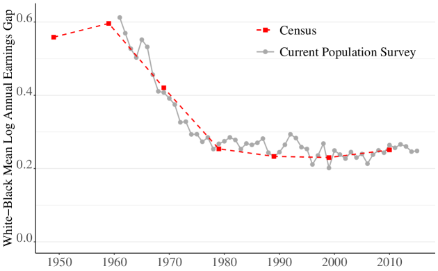
Figure 2: White-Black Unadjusted Wage Gap in the Long Run

Notes: This figure is a replication of Figure 1 in Derenoncourt and Montialoux, (2021). The data sources are the Current Population Survey 1962–2016, U.S. Census from 1950 to 2000, and American Community Survey data in 2010 and 2017. Sample includes black or white adults aged 25–65, who worked more than 13 weeks last year, worked three hours last week, do not live in group quarters, are not self-employed and not unpaid family worker with no missing industry or occupation code.

Recently, Derenoncourt and Montialoux, (2021) put forward a new explanation: the extension of the federal minimum wage to some industries. The Fair Labor Standards Act of 1966 established a federal minimum wage (effective February 1967) in previously unregulated industries, which employed about $20\%$ of the total workforce in the US and nearly a third of all black workers. They evaluate the minimum wage policy effect on earning, using a cross-industry difference-in-differences design, in which 7 treated and 8 control industries were subject to the minimum wage under the 1966 and 1938 Fair Labor Standards Act, respectively.

Using repeated cross-sections of black and white workers aged between 25 and 55 for year 1961 and 1963–1980, extracted from March CPS, they estimate the following two-way fixed effects mean regression model:

$$y_{ist}=\delta_{0}+\delta_{t}d_{st}+{z}_{ist}^{\prime}{\beta}+\phi_{s}+\nu_{t}+\eta_{ist},$$ (7)

for worker $i$ in industry $s=1,\dots,15$ and time $t=1961,1963\dots,1980$. Here, $y_{ist}$ is the log annual earning deflated by annual CPI-U-RS ($2017), and $d_{st}$ denotes a dummy variable taking 1 if industrial sector $s$ is subject to the federal minimum wage and 0 otherwise. Also, $z_{ist}$ is a vector of worker’s characteristics and unobserved random variables consist of industry fixed effect $\phi_{s}$, time fixed effect $\nu_{t}$ and an idiosyncratic error $\eta_{ist}$. The parameter of interest is $\delta_{t}$, which measures dynamic policy effects.

Their result shows that, after controlling for individual characteristics, the average wage of workers in the newly covered industries is around $5\%$ higher relative to that in control industries in 1967–1980 compared with the pre-period 1961–1966, and the effect of minimum wage reform on workers’ log-earning is more than twice as large for black workers as that for white workers on average. In addition to the above regression, they present several regression results to uncover intricate facets of the effects of minimum wage by taking various variables as the dependent variable in (7), including log annual wages or its unconditional quantiles, and also selecting sub-samples based on workers’ characteristics.

5.2 Model and Practical Implementation

We analyze time-varying policy effects from 1967 to 1980 at quantile $u\in\{0.1,0.3,0.5,0.7,0.9\}$. Following the original model in (7), we consider the following $u^{\mathrm{th}}$ quantile regression model in (1) with $\alpha_{st}(u)=[\alpha_{1st}(u),\dots,\alpha_{Jst}(u)]^{\prime}$, where, for $j=1,\dots,J$,

$$\alpha_{jst}(u)=\delta_{j0}(u)+\delta_{jt}(u)d_{st}+{f}_{jt}(u)^{\prime}{\lambda}_{js}(u)+\eta_{jst}(u).$$ (8)

Here, a set of coefficients $\{\delta_{jt}(u)\}_{t=1967}^{1980}$ measures the time-varying policy effect.

For simplicity of interpretation, we treat some of the original covariates as ordered variables rather than dummy variables for categories. More precisely, $z_{ist}$ includes a constant $1$, dummy variables for race (white/black), gender (male/female) and work type (full-time/part-time), and ordered variables including years of schooling, experience, experience squared, the number of weeks worked in a year, and the number of hours worked in a week. This selection yields a very similar result of the mean-regression in (7) as the one in Derenoncourt and Montialoux, (2021). See Figure 3.

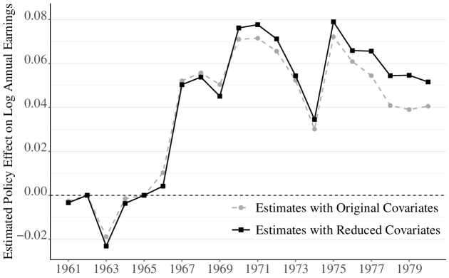
Figure 3: Estimation Results of Mean Regression

Notes: We plot the estimates of time-varying policy effect $\delta_{t}$ in Model (7) given the original set of controlled variables (in dashed grey line) and the estimates given the reduced set of covariates that used in our empirical analysis (in solid black line).

5.3 Results Analysis

In Figure 4, we present time-varying policy effects $\delta_{jt}(u)$ in (8) with $95\%$ confidence intervals for the categorical individual-level covariates. The policy effects for the continuous covariates eduction and experience are insignificant across quantiles. For presentation conciseness, those figures are omitted. Panel (a) reports the effects on the intercept coefficients, which correspond to white, male, full-time workers, which are insignificantly different from zero for most of the estimates. Panel (b) shows statistically significant positive policy effects for black workers in majority of the years across all quantiles. Especially, the policy effects are most significant at the 0.1th conditional quantile, which are 15–20% (0.15–0.2 log points). Panel (d) reports the estimated policy effects on the coefficient of the part-time dummy. Most of the estimates are positive but not statistically different from zero.

Panel (c) of Figure 4 presents the estimated policy effects on the female dummy’s coefficient. The effects in the late 1970s are positive and significant up to 0.7th quantile with a magnitude of 5%. However, caution is warranted in interpreting the results, which may be an integrated impact of the 1966 Fair Labor Standards Act and two pieces of important legislation that targeted labor market discrimination against women: the Equal Pay Act of 1963 and Title VII of the Civil Rights Act of 1964. Although the gender gap of median wages for full-time, full-year workers was unchanged over the 1960–1970s (see Blau and Kahn, , 2017), Bailey et al., (2021) recently document sharp increases in women’s wages relative to men’s below median during the 1960s. They underscore the importance of minimum wage policy and the laws to target gender-based workplace discrimination. Our result is consistent with their findings and furthermore suggests long-run positive effects even at 0.5th and 0.7th quantiles conditional on individual attributes.

Figure 4: Time-Varying Policy Effect Estimates ($\delta_{jt}$)

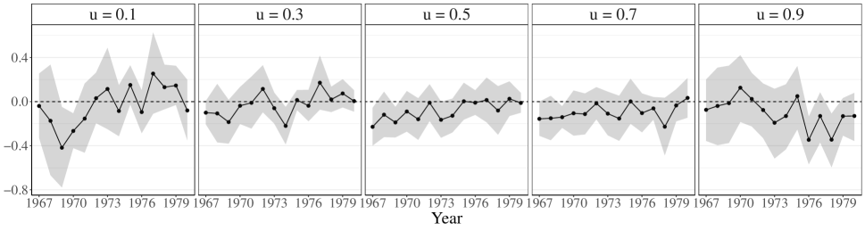
(a) Intercept (Base: White, Male, Full-Time Workers)

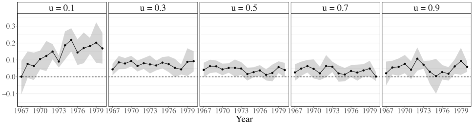
(b) Black

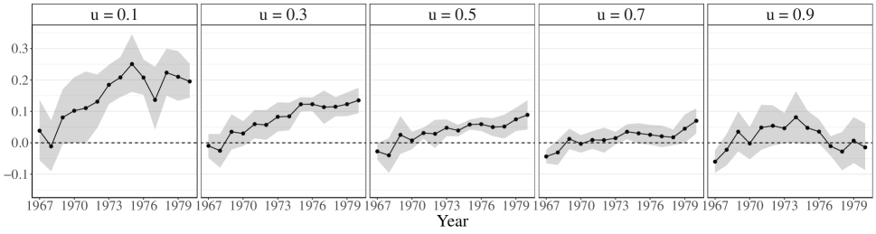
(c) Female

Notes: Panels (a)-(c) present the estimated time-varying marginal policy effect $\delta_{jt}(u)$ for $t=1967,\dots,1980$. From left to right, figures correspond to the estimates at quantiles $u=0.1,0.3,0.5,0.7,0.9$. Point estimates are plotted with solid black lines, and the pointwise $95\%$ confidence interval are shown as grey shaded area.

In Figure 5, we present estimated policy effects on changes in the within-inequality measure $\accentset{\mbox{\large.}}{\Delta}_{t}^{W}(u_{1},u_{2}|z)$ in the year $1980$. For quantile pairs $(u_{1},u_{2})=(0.1,0.9)$ or $(0.1,0.5)$, we measure how much the minimum wage policy changes the conditional quantile spread. For conditional variables $z$, we fix 12 years of education and 10 years of experience, while reporting three pairs of categorical individual attributes, as shown in the horizontal axis. The estimates suggest that the introduction of minimum wage reduces the within-inequality, while the reduction is statistically indistinguishable from 0 for all groups.

Figure 5: Changes in Within-Inequality in 1980

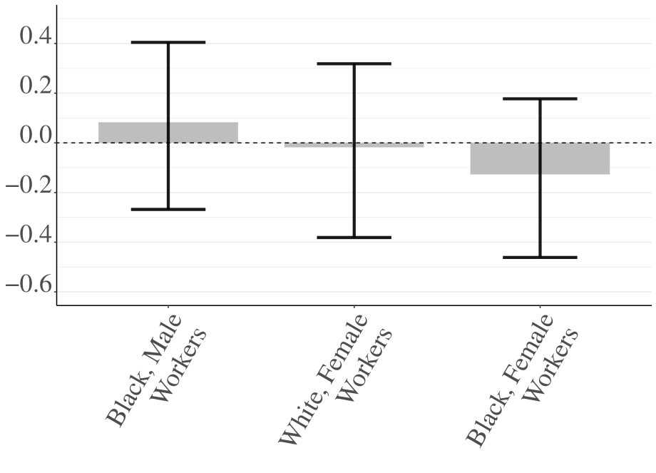
(a) $u_{1}=0.1,\ u_{2}=0.9$

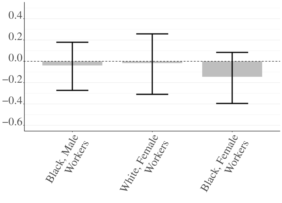
(b) $u_{1}=0.1,\ u_{2}=0.5$

Notes: Panels (a)-(b) report estimated changes in the within-inequality $\accentset{\mbox{\large.}}{\Delta}_{t}^{W}(u_{1},u_{2}|z)$ among individuals with attributes $z$ in year $t=1980$, with $(u_{1},u_{2})=(0.1,0.9)$ in Panel (a) and $(u_{1},u_{2})=(0.1,0.5)$ in Panel (b). The estimates are presented by grey bars with the $95\%$ confidence intervals in black. The horizontal axis shows the three subpopulations based on race and gender categories, while we fix 12 years of education and 10 years of experience.

Figure 6 reports the policy effects on the changes in the between-inequality measure, $\dot{\Delta}_{t}^{B}(u|z_{1},z_{2})$, for $t=1980$ and $u\in\{0.1,0.3,0.5,0.7,0.9\}$. The baseline $z_{2}$ is fixed to include white, male workers and $z_{1}$ changes over the three pairs of categorical attributes as in Figure 5, while the remaining variables are the same in $z_{1}$ and $z_{2}$. Panels (a) suggests significant negative impacts on the between-inequality for black, male workers, comparing to white, male workers, with magnitudes 5–20% for all quantiles excepts the 0.7 conditional quantile. Panels (b) also shows reduction (0.05–0.20) in the between-inequality for white, female workers at the 0.7th conditional quantile and below. Panels (c) plots results for female, black workers, and the estimated changes in the between-inequality range from -0.05 to -0.35 at the 0.7th conditional quantile and below.

Figure 6: Changes in Between-Inequality in 1980

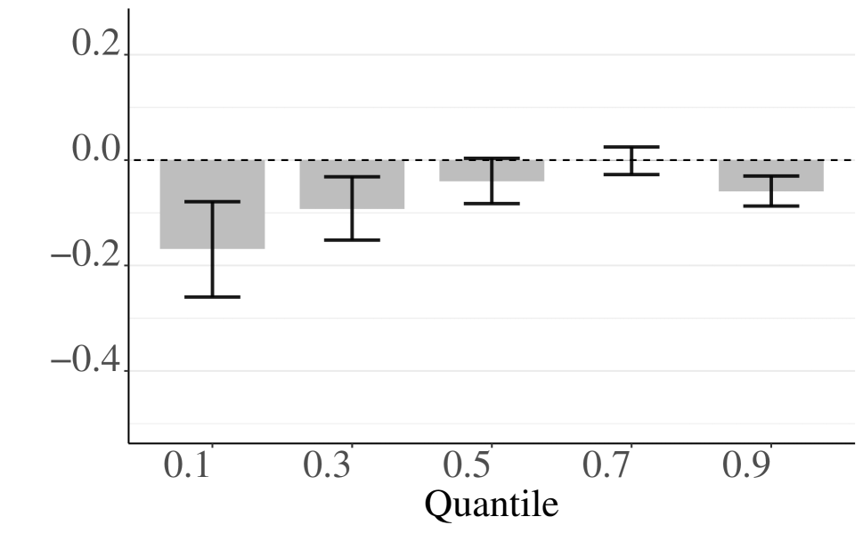
(a) Black, Male Workers

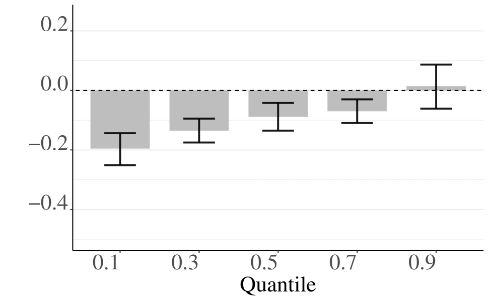
(b) White, Female Workers

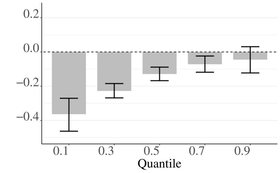
(c) Black, Female Workers

Notes: Panels (a)-(c) plot the changes in between-inequality ($\accentset{\mbox{\large.}}{\Delta}_{t}^{B}$) between multiple groups and the base-level group: white male workers (with 12 years of education and 10 years of experience) while holding other individual covariates constant. The inequality measure are considered at quantiles $u=0.1,0.3,0.5,0.7,0.9$ at year 1980. Point estimates are presented by grey bars with point-wise $95\%$ confidence intervals shown in black.

To illustrate the robustness of the significant policy-effects in reducing the between-equality, Figure 7 plots the changes in between-inequality for black, female workers from 1967 to 1980. In quantiles up to medium, the magnitude of reduction in the between-inequality increases as time increase. In addition, such policy effects are significant after 1970. Similar patterns are also witnessed in the other two groups presented in Figure 6. We choose not to report those plots for the concise of presentation.

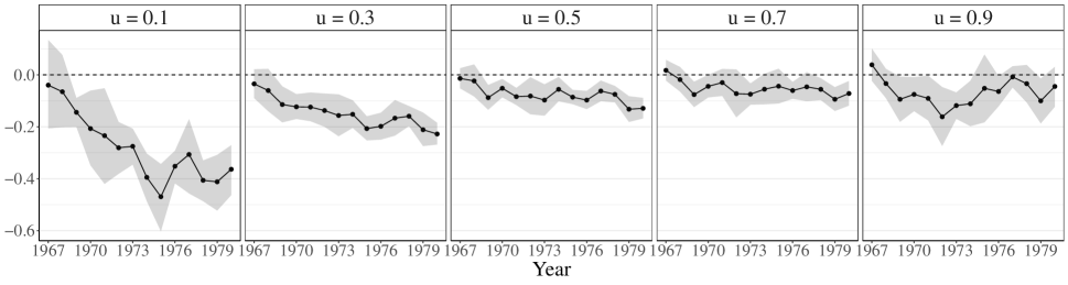
Figure 7: Changes in Between-Inequality for Black, Female Workers from 1967 to 1980

Notes: From left to right, figures correspond to the estimates at quantiles $u=0.1,0.3,0.5,0.7,0.9$. Point estimates are plotted with solid black lines, and the pointwise $95\%$ confidence interval are shown as grey shaded area.

Overall, the results above confirm the findings of Derenoncourt and Montialoux, (2021) that the reform was effective in improving the black economic status and reducing the racial income gap. In addition, we provide an empirical evidence of a compounded impact of the policy effect in reducing the racial and gender income gap, which leads to the significant reduction in the between-inequality at least up to the medium.

6 Conclusion

In this paper, we introduce an estimation method for evaluating the effect of group-level policies under the quantile regression framework with interactive fixed effects. Our method can capture the heterogeneous policy effects through the interaction of policy variables and the individual observed and unobserved characteristics, while controlling the unobserved interactive fixed effects, and provides a straightforward way of identifying the policy effect on inequality measures. The consistency and limiting distribution of the proposed estimators are established. Using our proposed model, we evaluate the effect of the minimum wage policy on earnings between 1967 and 1980 in the United States. Our analysis confirms the findings of Derenoncourt and Montialoux, (2021) that the policy helps reduce the racial income gap by improving the black economic status. On top of that, we provide empirical evidence of a compounded policy effect in narrowing the racial and gender gap, which contributes to the significant reduction in the between-inequality.

Appendix A Simulation Study

In this appendix, we investigate the accuracy of both the point and interval estimators of the policy parameter $\delta_{jt}(u)$ through Monte Carlo simulations. We consider two scenarios, where the unobserved factors are either correlated or uncorrelated with the group-level regressors.

A.1 Data Generating Process

We generate data according to the following model, for $i=1,...,N,\ s=1,...,S$, and $t=1,...,T$,

$$y_{ist}=\alpha_{st0}(u_{ist})+z_{ist}\alpha_{st1}(u_{ist}),\quad\alpha_{st1}=2+0.1u,$$

$$\alpha_{st0}(u_{ist})=\delta_{0}(u_{ist})+d_{st}\delta_{t}(u_{ist})+x_{st}\beta(u_{ist})+f_{t}(u_{ist})^{\prime}\lambda_{s}(u_{ist})+\eta_{st}(u_{ist}),$$

$$\delta_{0}(u)=2+\frac{u^{2}}{4},\quad\delta_{t}(u)=2+\frac{t}{2T}+\frac{u^{2}}{4},$$

where $\{u_{ist}\}$ and $\{\xi_{st}\}$ are i.i.d $\text{U}(0,1)$, $\{z_{ist}\}$ are i.i.d $\text{U}(0,1)$, $x_{st}$ are i.i.d $N(0,1)$, $(f_{t1},f_{t2})$ are generated orthogonally via the SVD of a $T\times T$ random matrix whose entries are i.i.d $N(0,1)$, and $(\lambda_{s1},\lambda_{s2})$ are generated from i.i.d ${\rm U}(0,2)$. The policy dummy variable $d_{st}=1\{t\geq T/4\}\times 1\{s\geq S/4\}$, that is, we fixed the first one quarter of the cross-sections as the control groups, and the policy is implemented at $T_{0}=T/4$.

We consider the following two scenarios in terms of whether exists endogenity in the group-level:

1. group-level observables $x_{st}$ are i.i.d $N(0,1)$.

2. group-level observables $x_{st}=\zeta_{st}+0.02f_{t1}^{2}+0.02\lambda_{s1}^{2}$, where $\{\zeta_{st}\}$ are i.i.d $N(0,1)$. This setting allows moderate endogeneity at group-level.

A.2 Performance of the Point Estimators

We investigate the accuracy of the point estimators of the policy parameters $\delta_{T}(u)$ for both scenarios. The sample bias and standard deviation at finite iteration steps $m=2,5$ and after convergence criterion satisfied are reported in Table 1.

The simulation shows a few nice properties, which can be summarized as follows. First of all, the recursive estimator converge quite fast. In all cases, the mean bias and standard deviation of the coefficient estimation at the second iteration are reasonably small. In addition, the estimators remain valid even if the number of observations per group ($N_{st}$) is relatively small comparing to the total number of groups and time ($S\times T$), which is a particular attractive property in practice.

Table 1: Sample Bias and Standard Deviation of estimates of the Policy Parameters

				Scenario 1			Scenario 2
$N$	$S$	$T$	$u$	$\widehat{\delta}^{(2)}_{T}(u)$	$\widehat{\delta}^{(5)}_{T}(u)$	$\widehat{\delta}_{T}(u)$	$\widehat{\delta}^{(2)}_{T}(u)$	$\widehat{\delta}^{(5)}_{T}(u)$	$\widehat{\delta}_{T}(u)$
500	40	25	0.1	$0.003\ (0.074)$	$0.001\ (0.017)$	$0.001\ (0.016)$	$0.005\ (0.084)$	$0.002\ (0.017)$	$0.001\ (0.016)$
			0.5	$0.001\ (0.031)$	$0.001\ (0.015)$	$0.001\ (0.014)$	$0.003\ (0.035)$	$0.001\ (0.015)$	$0.001\ (0.014)$
			0.9	$0.005\ (0.041)$	$0.003\ (0.014)$	$0.001\ (0.014)$	$-0.003\ (0.085)$	$-0.003\ (0.028)$	$-0.002\ (0.028)$
	40	50	0.1	$0.003\ (0.041)$	$0.001\ (0.025)$	$0.001\ (0.014)$	$0.003\ (0.038)$	$0.001\ (0.008)$	$0.001\ (0.008)$
			0.5	$0.003\ (0.031)$	$0.001\ (0.014)$	$0.001\ (0.014)$	$0.001\ (0.012)$	$0.001\ (0.007)$	$0.001\ (0.007)$
			0.9	$0.002\ (0.035)$	$0.003\ (0.034)$	$-0.001\ (0.014)$	$0.003\ (0.041)$	$-0.001\ (0.012)$	$-0.001\ (0.011)$
1000	40	50	0.1	$0.006\ (0.041)$	$0.003\ (0.035)$	$0.002\ (0.014)$	$-0.005\ (0.076)$	$0.001\ (0.013)$	$0.001\ (0.012)$
			0.5	$0.004\ (0.051)$	$-0.003\ (0.035)$	$0.001\ (0.014)$	$-0.001\ (0.029)$	$0.001\ (0.012)$	$0.001\ (0.012)$
			0.9	$0.003\ (0.031)$	$0.001\ (0.015)$	$-0.001\ (0.014)$	$-0.004\ (0.087)$	$-0.001\ (0.026)$	$-0.001\ (0.025)$
	60	50	0.1	$0.006\ (0.081)$	$0.002\ (0.015)$	$0.001\ (0.014)$	$0.004\ (0.037)$	$0.001\ (0.005)$	$0.001\ (0.005)$
			0.5	$0.005\ (0.031)$	$0.003\ (0.015)$	$0.001\ (0.014)$	$0.001\ (0.010)$	$0.001\ (0.005)$	$0.001\ (0.005)$
			0.9	$0.002\ (0.041)$	$-0.002\ (0.015)$	$0.001\ (0.014)$	$-0.001\ (0.041)$	$0.001\ (0.010)$	$0.001\ (0.010)$
2000	60	50	0.1	$0.005\ (0.070)$	$0.001\ (0.010)$	$0.001\ (0.009)$	$0.005\ (0.070)$	$0.001\ (0.011)$	$0.001\ (0.009)$
			0.5	$0.004\ (0.070)$	$0.003\ (0.014)$	$0.002\ (0.008)$	$-0.003\ (0.029)$	$0.001\ (0.010)$	$0.001\ (0.010)$
			0.9	$0.002\ (0.070)$	$-0.001\ (0.011)$	$0.001\ (0.009)$	$0.004\ (0.084)$	$0.001\ (0.026)$	$0.001\ (0.025)$
	80	50	0.1	$0.002\ (0.070)$	$0.001\ (0.011)$	$0.001\ (0.009)$	$0.001\ (0.037)$	$0.001\ (0.004)$	$0.001\ (0.004)$
			0.5	$0.002\ (0.064)$	$0.001\ (0.010)$	$0.001\ (0.007)$	$0.001\ (0.011)$	$0.001\ (0.005)$	$0.001\ (0.005)$
			0.9	$0.001\ (0.068)$	$0.001\ (0.011)$	$0.001\ (0.010)$	$0.002\ (0.039)$	$-0.001\ (0.010)$	$-0.001\ (0.010)$

Notes: The number of Monte-Carlo repetitions is 250. We report bias averaged over 250 repetitions with the standard deviation in the parenthesis.

A.3 Performance of the Interval Estimators

For the interval accuracy, we report the coverage rate of the confidence interval when the estimates converge. The coverage rate is calculated by the ratio of $\delta_{T}(u)$ within the $95\%$ confidence interval under $250$ simulation repetitions. The estimated asymptotic bias and covariance are computed according to Corollary 4.2.

Table 2 demonstrates that the confidence interval is conservative (around $0.9$) when sample size is modest, while the coverage rate gradually increases to $0.93$ when the sample size $(N_{\min},S,T)$ increases.

Table 2: Coverage Rate of the $95\%$ Confidence Interval for $\delta_{T}(u)$

			Scenario 1			Scenario 2
N	S	T	$u=0.1$	$u=0.5$	$u=0.9$	$u=0.1$	$u=0.5$	$u=0.9$
500	40	25	0.896	0.903	0.907	0.892	0.900	0.900
	40	50	0.900	0.900	0.904	0.900	0.900	0.904
1000	40	50	0.895	0.899	0.902	0.899	0.903	0.899
	60	50	0.892	0.903	0.903	0.896	0.907	0.907
2000	60	50	0.923	0.911	0.915	0.921	0.911	0.920
	80	50	0.915	0.947	0.922	0.915	0.955	0.922

Notes: Coverage rate based on 250 simulation repetitions.

Appendix B Proof of Theorems

In this appendix, we present the proofs of the results on the main model (1)-(2). Specifically, the proof of identification theorem of treatment parameters (Theorems 2.1) is established in Section B.1. The asymptotic properties in Section 4.2 are given in Section B.2. All the preliminary lemmas required in Section B.2 are established and proved proceeding appendices.

In what follows, we use a few additional notation. For a square matrix $A$, let $\text{tr}(A)$ denote the trace operation of $A$ and let $\rho_{\max}(A)$ and $\rho_{\min}(A)$ denote the maximum and minimum eigenvalue of $A$, respectively. Notice that $\rho_{\max}(A)\leq\text{tr}(A)$ for every symmetric positive semi-definite matrix. Thus, $\|X\|^{2}\leq\text{tr}(X^{\prime}X)$ for matrix $X$, and we repeatedly use this inequality. We denote $c$ and $C$ as strictly positive constants that depend only on $c_{M},\ C_{M}$, whose values can change at each appearance. Let ${x}_{st},{x}_{s(k)}$ and $x_{st(k)}$ represent different vectors related to the regressor $X$. Precisely, ${x}_{st}$ is a $K\times 1$ vector, ${x}_{s(k)}$ is a $T\times 1$ vector and $x_{st(k)}$ is a scalar for any $(s,t,k)\in\{1,...,S\}\times\{1,...,T\}\times\{1,...,K\}$. Let $\delta_{ST}\equiv\min(\sqrt{S},\sqrt{T})$. Let $e_{k}$ denote the a column vector, whose entries are all $0$ except for the $k$-th entry; the dimension of $e_{k}$ varies along with the context.

B.1 Proof of the Identification Theorem

Proof of Theorem 2.1.

Let $u\in\mathcal{U}$, $z\in\mathcal{Z}$ and $t\geq T_{0}$ be fixed. Under the potential outcome framework (3)-(4), we can write $\Delta_{t}^{AQTT}(u|z)=z^{\prime}\mathbb{E}[\alpha_{st}^{1}(u)-\alpha_{st}^{0}(u)|d_{s}=1]$. Under Assumption 2.3.(i), it follows from (4) that $\mathbb{E}[\alpha_{jst}^{1}(u)-\alpha_{jst}^{0}(u)|d_{s}=1]=\mathbb{E}[\Delta_{jst}(u)|d_{s}=1]$, for $j=1,...,J$. Thus, it is straightforward that $\Delta_{t}^{AQTT}(u|z)=z^{\prime}\mathbb{E}[\Delta_{st}(u)|d_{s}=1]$, $\accentset{\mbox{\large.}}{\Delta}_{t}^{W}(u_{1},u_{2}|z)=z^{\prime}\mathbb{E}[\Delta_{st}(u_{2})-\Delta_{st}(u_{1})|d_{s}=1]$, and $\accentset{\mbox{\large.}}{\Delta}_{t}^{B}(u|z_{1},z_{2})=(z_{2}-z_{1})^{\prime}\mathbb{E}[\Delta_{st}(u)|d_{s}=1]$, where $\Delta_{st}(u):=[\Delta_{1st}(u),...,\Delta_{Jst}(u)]^{\prime}$.

Moreover, under the potential outcome framework, we have $\alpha_{jst}(u)=(1-d_{st})\alpha_{jst}^{0}(u)+d_{st}\alpha_{jst}^{1}(u)$ . Therefore, we can rewrite (4) as

$$\alpha_{jst}(u)=d_{st}\mathbb{E}[\Delta_{jst}(u)|d_{s}=1]+x_{st}^{\prime}\beta_{j}(u)+f_{jt}(u)^{\prime}\lambda_{js}(u)+\eta_{jst}(u)$$ (9)

where $\eta_{jst}(u):=d_{st}(\Delta_{jst}(u)-\mathbb{E}[\Delta_{jst}(u)|d_{s}=1])+(1-d_{st})\eta_{jst}^{0}(u)+d_{st}\eta_{jst}^{1}(u)$. Then, it is clear that (9) coincides with (2) by defining $\delta_{jt}(u):=\mathbb{E}[\Delta_{jst}(u)|d_{s}=1]$.

To prove the theorem, it remains to check that $\delta_{jt}(u)$ can be identified from model (1)-(2) for each $j=1,\dots,J$ and $t\geq T_{0}$.

It is know that, for model (1)-(2), under Assumption 2.1, we can estimate the quantile regression coefficients $\alpha_{jst}(u)$ from model (1). Also, we can identify the regression coefficients, factors and factor loadings, using the argument of Bai, (2009) under Assumption 2.2. Thus, we treat the quantile regression coefficients, factors and loadings as known objects in the rest of the proof. Then, since $\mathbb{E}[\eta_{jst}(u)|d_{st},X_{s}]=0$ under Assumption 2.3, taking the expectation on both sides of (2) leads to the normal equations

$$\mathbb{E}[d_{st}(\alpha_{jst}-f_{jt}(u)^{\prime}\lambda_{js}(u))]=\mathbb{E}[d_{st}^{2}]\delta_{jt}(u)+\mathbb{E}[d_{st}x_{st}^{\prime}]\beta_{j}(u),$$ (10)

$$\mathbb{E}[x_{st}(\alpha_{jst}-f_{jt}(u)^{\prime}\lambda_{js}(u))]=\mathbb{E}[d_{st}x_{st}]\delta_{jt}(u)+\mathbb{E}[x_{st}x_{st}^{\prime}]\beta_{j}(u).$$ (11)

Solving (11) with respect to $\beta_{j}(u)$, we have $\beta_{j}(u)=\mathbb{E}[x_{st}x_{st}^{\prime}]^{-1}\{\mathbb{E}[x_{st}(\alpha_{jst}-f_{jt}(u)^{\prime}\lambda_{js}(u))]-\mathbb{E}[d_{st}x_{st}]\delta_{jt}(u)\}$ given that $\mathbb{E}[x_{st}x_{st}^{\prime}]^{-1}$ is invertible under Assumption 2.2.(ii). Substituting the solution into (10), we obtain

$$\delta_{jt}(u)=\mathbb{E}[d_{st}\Pi_{st}]^{-1}\mathbb{E}[\Pi_{st}(\alpha_{jst}(u)-f_{jt}(u)^{\prime}\lambda_{js}(u))],$$

where $\Pi_{st}:=d_{st}-\mathbb{E}[d_{st}x_{st}^{\prime}]\mathbb{E}[x_{st}x_{st}^{\prime}]^{-1}x_{st}$. Moreover, since $\text{Var}(x_{st})=\mathbb{E}[x_{st}x_{st}^{\prime}]-\mathbb{E}[x_{st}]\mathbb{E}[x_{st}^{\prime}]>0$, it follows that $\mathbb{E}[d_{st}\Pi_{st}]=\mathbb{E}[\mathbb{E}[d_{st}\Pi_{st}]|d_{st}]=\mathbb{P}(d_{st}=1)(1-\mathbb{E}[x_{st}^{\prime}]\mathbb{E}[x_{st}x_{st}^{\prime}]^{-1}\mathbb{E}[x_{st}])>0,$ that is, $\mathbb{E}[d_{st}\Pi_{st}]$ is invertible.

In summary, $\delta_{jt}(u)$ is identifiable in model (1)-(2). Consequently, the policy parameters $\Delta_{t}^{AQTT}(u|z)$, $\accentset{\mbox{\large.}}{\Delta}_{t}^{B}(u|z_{1},z_{2})$ and $\accentset{\mbox{\large.}}{\Delta}_{t}^{W}(u_{1},u_{2}|z)$ are identifiable, following the arguments at the beginning of the proof ∎

B.2 Proofs of the Asymptotic Properties

In what follows, we use the following facts: for all $(s,t)\in\{1,...,S\}\times\{1,...,T\}$, $\|X_{s}\|=O_{p}(\sqrt{T})$, $\|F_{j}(u)\|=O_{p}(\sqrt{T})$, $\|\widehat{F}_{j}^{(m)}(u)\|=O_{p}(\sqrt{T})$, $\|\Lambda_{j}(u)\|=O_{p}(\sqrt{S})$, $\|\widehat{\Lambda}_{j}^{(m)}(u)\|=O_{p}(\sqrt{S})$ under Assumption 4.1. Also, $\|M_{F_{j}}(u)\|=O_{p}(1)$ since the largest eigenvalue of $M_{F_{j}}(u)$ is 1 as $M_{F_{j}}(u)$ is a projection matrix, and similarly, $\|M_{\widehat{F}_{j}}^{(m)}(u)\|=O_{p}(1)$. In addition, we define the orthogonal projection matrix $P_{F_{j}}(u):={F_{j}}(u)({F_{j}}(u)^{\prime}{F_{j}}(u))^{-1}{F_{j}}(u)$.

Before proceeding to the proof, since the convergence of $\widehat{\delta}^{(m)}_{jt}(u)$ and $\widehat{\beta}^{(m)}_{j}(u)$ are different, there is a need to partial-out the expression of $\widehat{\delta}^{(m)}_{jt}(u)$ and $\widehat{\beta}^{(m)}_{j}(u)$ from that of $\widehat{\beta}^{(m)}_{j}(u):=[\widehat{\delta}^{(m)}_{jT_{0}}(u),...,\widehat{\delta}^{(m)}_{jT}(u),\widehat{\beta}^{(m)}_{j}(u)]^{\prime}$ obtained in Section 3. Recall that the estimator $\widehat{\beta}^{(m)}_{j}(u)$ is the minimizer of the SSR of Equation (5). Therefore, by setting the first order derivative of SSR with respect to $\beta^{(m)}_{j}(u)$ to zero, we obtain the following relationships between $\widehat{\delta}^{(m)}_{jt}(u)$ and $\widehat{\beta}^{(m)}_{j}(u)$:

$$\begin{cases}\widehat{\delta}_{jt}^{(0)}(u)=\big{(}\sum_{s=1}^{S}d_{s}^{2}\big{)}^{-1}\sum_{s=1}^{S}d_{s}\big{(}\widehat{\alpha}_{jst}(u)-x_{st}^{\prime}\widehat{\beta}_{j}^{(0)}(u)\big{)},\quad t=T_{0},...,T,\\ \widehat{\beta}_{j}^{(0)}(u)=\big{(}\sum_{s=1}^{S}X_{s}^{\prime}X_{s}\big{)}^{-1}\sum_{s=1}^{S}X_{s}^{\prime}\big{(}\widehat{A}_{js}(u)-D_{s}\widehat{\delta}_{j}^{(0)}(u)\big{)},\end{cases}$$ (12)

and, for $m\geq 1$, given $(\widehat{F}_{j}^{(m)}(u),\widehat{\Lambda}^{(m)}_{j}(u))$,

$$\begin{cases}\widehat{\delta}_{jt}^{(m)}(u)=\big{(}\sum_{s=1}^{S}d_{s}^{2}\big{)}^{-1}\sum_{s=1}^{S}d_{s}\big{(}\widehat{\alpha}_{jst}(u)-x_{st}^{\prime}\widehat{\beta}_{j}^{(m)}(u)-\widehat{f}^{(m)}_{jt}(u)^{\prime}\widehat{\lambda}^{(m)}_{js}(u)\big{)},\\ \widehat{\beta}_{j}^{(m)}(u)=\big{(}\sum_{s=1}^{S}X_{s}^{\prime}X_{s}\big{)}^{-1}\sum_{s=1}^{S}X_{s}^{\prime}\big{(}\widehat{A}_{js}(u)-D_{s}\widehat{\delta}_{j}^{(m)}(u)-\widehat{F}^{(m)}_{j}(u)\widehat{\lambda}^{(m)}_{js}(u)\big{)}.\end{cases}$$ (13)

Using the above relationships, we present the proof of Theorem 4.1 as follows.

Proof of Theorem 4.1.

Since $u$ and $j$ are fixed, we suppress $u$ and $j$ throughout the following proof. The proof is completed by induction. We first show that (i) $\sqrt{ST}\|\widehat{\beta}^{(0)}-{\beta}\|=O_{P}(1)$, $\sqrt{S}|\widehat{\delta}^{(0)}_{t}-{\delta}_{t}|=O_{P}(1)$, and $\sqrt{S/T}|\sum_{t=1}^{T_{0}}\widehat{\delta}^{(0)}_{t}-{\delta}_{t}|=O_{P}(1)$. Then, using the iterative formula and the rates of the previous estimators, we show that suppose the above rates hold at $(m-1)^{\text{th}}$ iteration, then the rates hold at $m^{\text{th}}$ iteration for all $m\geq 1$.

(i) We start with $\widehat{\beta}^{(0)}-{\beta}$. By simple algebra on (12) and the linear model (2) for $\alpha_{st}$, we obtain

$$\begin{cases}\widehat{\delta}_{t}^{(0)}-\delta_{t}=\big{(}\sum_{s=1}^{S}d_{s}^{2}\big{)}^{-1}\sum_{s=1}^{S}d_{s}\big{(}(\widehat{\alpha}_{st}-\alpha_{st})-w_{st}^{\prime}(\widehat{\beta}^{(0)}-\beta)+f_{t}^{\prime}\lambda_{s}+\eta_{st}\big{)},\\ \widehat{\beta}^{(0)}-\beta=\big{(}\sum_{s=1}^{S}X_{s}^{\prime}X_{s}\big{)}^{-1}\sum_{s=1}^{S}X_{s}^{\prime}\big{(}(\widehat{A}_{s}-A_{s})-D_{s}(\widehat{\delta}^{(0)}-\delta)+F\lambda_{s}+\eta_{s}\big{)}.\end{cases}$$ (14)

By further substituting the expression of $\widehat{\delta}_{t}^{(0)}-\delta_{t}$ ($t=T_{0},...,T$) into $\widehat{\beta}^{(0)}-\beta$, we obtain

$$\Big{[}\sum_{s=1}^{S}X_{s}^{\prime}X_{s} -\Big{(}\sum_{s=1}^{S}d_{s}^{2}\Big{)}^{-1}\sum_{s,g=1}^{S}X_{s}^{\prime}D_{s}D_{g}^{\prime}X_{g}\Big{]}\big{(}\widehat{\beta}^{(0)}-\beta\big{)}$$

$$=\sum_{s=1}^{S}X_{s}^{\prime}[(\widehat{A}_{s}-A_{s})+F\lambda_{s}+\eta_{s}]-\Big{(}\sum_{s=1}^{S}d_{s}^{2}\Big{)}^{-1}\sum_{s,g=1}^{S}X_{s}^{\prime}D_{s}D_{g}^{\prime}[(\widehat{A}_{g}-A_{g})+F\lambda_{g}+\eta_{g}].$$

An application of the triangle inequality together with Lemma C.1 yields $\big{\|}\sum_{s=1}^{S}X_{s}^{\prime}\big{(}\widehat{{A}}_{s}-A_{s}\big{)}\big{\|}=O_{P}((ST)^{1/4}).$ Also, $(ST)^{-1}\sum_{s=1}^{S}X_{s}^{\prime}F\lambda_{s}=O_{P}\big{(}\sqrt{ST}\big{)}$ and (29) in Lemma C.2 shows that $(ST)^{-1/2}\sum_{s=1}^{S}X_{s}^{\prime}\eta_{s}=O_{P}(1)$. In addition, recall that $D_{s}=d_{s}[e_{T_{0}},...,e_{T}]$ and $d_{s}\in\{0,1\}$, we then have

$$\Big{\|}\sum_{s,g=1}^{S}X_{s}^{\prime}D_{s}D_{g}^{\prime}(\widehat{A}_{g}-A_{g})\Big{\|}=\sup_{g,t}|\widehat{\alpha}_{gt}-\alpha_{gt}|\cdot\sum_{s,g=1}^{S}\sum_{t=T_{0}}^{T}\|x_{st}d_{s}d_{g}\|=O_{P}(S^{5/4}T^{1/4}),$$

following from Lemma C.1,

$$\Big{\|}\sum_{s,g=1}^{S}X_{s}^{\prime}D_{s}D_{g}F\lambda_{g}\Big{\|}\leq\Big{(}\sum_{t=T_{0}}^{T}\Big{\|}\sum_{s=1}^{S}d_{s}w_{st}\Big{\|}^{2}\Big{)}^{1/2}\Big{(}\sum_{t=T_{0}}^{T}\Big{\|}\sum_{g=1}^{S}d_{s}f_{t}^{\prime}\lambda_{g}\Big{\|}^{2}\Big{)}^{1/2}=O_{P}(ST),$$

due to the assumption that $\mathbb{E}\|\sum_{g=1}^{S}d_{s}f_{t}^{\prime}\lambda_{g}\|^{2}=O_{P}(S)$ for all $t\geq T_{0}$ uniformly, and,

$$\Big{\|}\sum_{s,g=1}^{S}X_{s}^{\prime}D_{s}D_{g}\eta_{g}\Big{\|}=\Big{\|}\sum_{s,g=1}^{S}\sum_{t=T_{0}}^{T}d_{s}d_{g}x_{st}\eta_{gt}\Big{\|}=O_{P}(S\sqrt{T})$$

by $\alpha$-mixing. Finally, under Assumption 4.5, we have $\|(\sum_{s=1}^{S}d_{s}^{2})^{-1}\|=O_{P}(S^{-1})$, and $\|[\sum_{s=1}^{S}X_{s}^{\prime}X_{s}-(\sum_{s=1}^{S}d_{s}^{2})^{-1}\sum_{s,g=1}^{S}X_{s}^{\prime}D_{s}D_{g}^{\prime}X_{g}]^{-1}\|=O_{P}((ST)^{-1})$. Thus, we collect the rates for all terms and obtain $\sqrt{ST}\|\widehat{\beta}^{(0)}_{j}(u)-{\beta}_{j}(u)\|=O_{P}(1)$.

(ii) We then consider $\widehat{\delta}^{(0)}_{t}-{\delta}_{t}$ for a given $t\geq T_{0}$. We check all the terms of the expression of $\widehat{\delta}^{(0)}_{t}-{\delta}_{t}$ in (14) as follows: $|\sum_{s=1}^{S}d_{s}(\widehat{\alpha}_{st}-\alpha_{st})|\leq\sup_{s,t}|\widehat{\alpha}_{st}-\alpha_{st}|\cdot\sum_{s=1}|d_{s}|=O_{P}(S^{1/4}T^{-3/4})$ using Lemma C.1, $|\sum_{s=1}^{S}d_{s}f_{t}^{\prime}\lambda_{s}|=O_{P}(\sqrt{S})$ by assumption, $|\sum_{s=1}^{S}d_{s}\eta_{st}|=O_{P}(\sqrt{S})$ by $\alpha$-mixing, and $|\sum_{s=1}^{S}d_{s}x_{st}^{\prime}(\widehat{\beta}^{(0)}-\beta)|\leq\|\widehat{\beta}^{(0)}_{j}(u)-{\beta}_{j}(u)\|\sum_{s=1}^{S}|x_{st}|=O_{P}(\sqrt{S/T})$. Finally, since $|(\sum_{s=1}^{S}d_{s}^{2})^{-1}\|=O_{P}(S^{-1})$ under Assumption 4.5, collecting the rates of all terms yields $\sqrt{S}|\widehat{\delta}^{(0)}_{jt}(u)-{\delta}_{jt}(u)|=O_{P}(1)$.

In addition, we show that $|\sum_{t=T_{0}}^{T}\widehat{\delta}^{(0)}_{jt}(u)-{\delta}_{jt}(u)|=O_{P}(1)$ as follows. Since

$$\sum_{t=T_{0}}^{T}\widehat{\delta}^{(0)}_{t}-{\delta}_{t}=\big{(}\sum_{s=1}^{S}d_{s}^{2}\big{)}^{-1}\sum_{s=1}^{S}\sum_{t=T_{0}}^{T}d_{s}\big{(}(\widehat{\alpha}_{st}-\alpha_{st})-w_{st}^{\prime}(\widehat{\beta}^{(0)}-\beta)+f_{t}^{\prime}\lambda_{s}+\eta_{st}\big{)},$$

applying similar arguments as those in (ii), it is easy to check that $|\sum_{s=1}^{S}\sum_{t=T_{0}}^{T}d_{s}(\widehat{\alpha}_{st}-\alpha_{st})|=O_{P}((ST)^{1/4})$, $|\sum_{s=1}^{S}\sum_{t=T_{0}}^{T}d_{s}x_{st}^{\prime}(\widehat{\beta}^{(0)}-\beta)|=O_{P}(\sqrt{ST})$, $|\sum_{s=1}^{S}\sum_{t=T_{0}}^{T}d_{s}f_{t}^{\prime}\lambda_{s}|=O_{P}(\sqrt{ST})$, and $|\sum_{s=1}^{S}\sum_{t=T_{0}}^{T}d_{s}\eta_{st}|=O_{P}(\sqrt{ST})$. Therefore, we have

$$\bigg{|}\sum_{t=T_{0}}^{T}\widehat{\delta}^{(0)}_{t} -{\delta}_{t}\bigg{|}$$

$$\leq O_{P}(S^{-1})\cdot\bigg{|}\sum_{s=1}^{S}\sum_{t=T_{0}}^{T}d_{s}\big{(}(\widehat{\alpha}_{st}-\alpha_{st})-x_{st}^{\prime}(\widehat{\beta}^{(0)}-\beta)+f_{t}^{\prime}\lambda_{s}+\eta_{st}\big{)}\bigg{|}=O_{P}(1).$$ (15)

We also note that a similar argument yields that $\|\sum_{t=T_{0}}^{T}\widehat{f}^{(1)}_{t}(\widehat{\delta}^{(0)}_{t}-\delta_{t})\|=O_{P}(1)$.

Now, for a given $m\geq 1$, suppose that $\sqrt{ST}\|\widehat{\beta}^{(m-1)}-{\beta}\|=O_{P}(1)$, $\sqrt{S}|\widehat{\delta}^{(m-1)}_{t}-{\delta}_{t}|=O_{P}(1)$, $|\sum_{t=T_{0}}^{T}\widehat{\delta}^{(m-1)}_{t}-{\delta}_{t}|=O_{P}(1)$ and $\|\sum_{t=T_{0}}^{T}\widehat{f}^{(m)}_{t}(\widehat{\delta}^{(m-1)}_{t}-\delta_{t})\|=O_{P}(1)$.

(iii) We want to show $\sqrt{ST}\|\widehat{\beta}^{(m)}-{\beta}\|=O_{P}(1)$. By simple algebra on (13) and the linear model for $\alpha_{st}$, we obtain

$$\Big{[}\sum_{s=1}^{S}X_{s}^{\prime}X_{s} -\Big{(}\sum_{s=1}^{S}d_{s}^{2}\Big{)}^{-1}\sum_{s,g=1}^{S}X_{s}^{\prime}D_{s}D_{g}^{\prime}X_{g}\Big{]}\big{(}\widehat{\beta}^{(m)}-\beta\big{)}$$

$$= \sum_{s=1}^{S}X_{s}^{\prime}\big{[}(\widehat{A}_{s}-A_{s})+\big{(}F\lambda_{s}-\widehat{F}^{(m)}\widehat{\lambda}^{(m)}_{s}\big{)}+\eta_{s}\big{]}$$

$$-\Big{(}\sum_{s=1}^{S}d_{s}^{2}\Big{)}^{-1}\sum_{s,g=1}^{S}X_{s}^{\prime}D_{s}D_{g}\big{[}(\widehat{A}_{g}-A_{g})+\big{(}F\lambda_{g}-\widehat{F}^{(m)}\widehat{\lambda}^{(m)}_{g}\big{)}+\eta_{g}\big{]},$$ (16)

and

$$\widehat{\delta}_{t}^{(m)}-\delta_{t}=\big{(}\sum_{s=1}^{S}d_{s}^{2}\big{)}^{-1}\sum_{s=1}^{S}d_{s}\big{(}(\widehat{\alpha}_{st}-\alpha_{st})-x_{st}^{\prime}(\widehat{\beta}^{(m)}-\beta)+\big{(}f_{t}^{\prime}\lambda_{s}-\widehat{f}^{(m)\prime}_{t}\widehat{\lambda}^{(m)}_{s}\big{)}+\eta_{st}\big{)}.$$ (17)

To find the rate of $\widehat{\beta}^{(m)}_{j}(u)-{\beta}_{j}(u)$, we derive the rates for all terms on the right-hand side of (B.2) below. As show in part (i), we have $\|\sum_{s=1}^{S}X_{s}^{\prime}[(\widehat{A}_{s}-A_{s})+\eta_{s}]\|=O_{P}(\sqrt{ST})$. We now consider the term $\sum_{s=1}^{S}X_{s}^{\prime}(F\lambda_{s}-\widehat{F}^{(m)}\widehat{\lambda}^{(m)}_{s})$. Using the expression that $\widehat{\lambda}^{(m)}_{s}=T^{-1}\widehat{F}^{(m)\prime}(\widehat{A}_{s}-D_{s}\widehat{\delta}^{(m)}-X_{s}\widehat{\beta}^{(m)})$, we obtain

$$\sum_{s=1}^{S}X_{s}^{\prime}(F\lambda_{s}-\widehat{F}^{(m)}\widehat{\lambda}^{(m)}_{s})= \sum_{s=1}^{S}X_{s}^{\prime}(F-\widehat{F}^{(m)}H^{(m)})\lambda_{s}+\sum_{s=1}^{S}X_{s}^{\prime}\widehat{F}^{(m)}(H^{(m)}\lambda_{s}-\widehat{\lambda}^{(m)}_{s})$$

$$= -\sum_{s=1}^{S}X_{s}^{\prime}P^{(m)}_{\widehat{F}}(\widehat{A}_{s}-A_{s})-\sum_{s=1}^{S}X_{s}^{\prime}P^{(m)}_{\widehat{F}}\eta_{s}$$

$$+\sum_{s=1}^{S}X_{s}^{\prime}P^{(m)}_{\widehat{F}}X_{s}(\widehat{\beta}^{(m-1)}-\beta)+\sum_{s=1}^{S}X_{s}^{\prime}P^{(m)}_{\widehat{F}}D_{s}(\widehat{\delta}^{(m-1)}-\delta)$$

$$+\sum_{s=1}^{S}X_{s}^{\prime}M^{(m)}_{\widehat{F}}(F-\widehat{F}^{(m)}H^{(m)})\lambda_{s},$$ (18)

where

$$H_{j}^{(m)}(u)= \widehat{\Upsilon}_{j}^{(m)}(u)\left({K}_{j}^{(m)}(u)\right)^{-1},$$ (19)

in which $\widehat{\Upsilon}_{j}^{(m)}(u)$ is the $r\times r$ diagonal matrix with diagonal elements being the $r$ largest eigenvalues of $\widehat{L}_{j}\big{(}\widehat{\delta}^{(m-1)}_{j}(u),\widehat{\beta}^{(m-1)}_{j}(u)\big{)}$, defined in (6), in descending order, and

$$K^{(m)}_{j}(u)= \bigg{(}\frac{\Lambda_{j}(u)^{\prime}\Lambda_{j}(u)}{S}\bigg{)}\bigg{(}\frac{F_{j}(u)^{\prime}\widehat{F}^{(m)}_{j}(u)}{T}\bigg{)}.$$

Now, we consider each term in the second equation of (B.2). For the first three terms, by Hölder’s and triangle inequalities, it is straightforward to show

$$\Big{\|}\sum_{s=1}^{S}X_{s}^{\prime}P^{(m)}_{\widehat{F}}(\widehat{A}_{s}-A_{s})\Big{\|}\leq\sup_{s}\|\widehat{A}_{s}-A_{s}\|\cdot\sum_{s=1}^{S}\|X_{s}\|\cdot\|P^{(m)}_{\widehat{F}}\|=O_{P}((ST)^{1/4}),$$

$$\Big{\|}\sum_{s=1}^{S}X_{s}^{\prime}P^{(m)}_{\widehat{F}}X_{s}(\widehat{\beta}^{(m-1)}-\beta)\Big{\|}\leq\sum_{s=1}^{S}\|X_{s}\|^{2}\cdot\|P^{(m)}_{\widehat{F}}\|\cdot\|\widehat{\beta}^{(m-1)}-\beta\|=O_{P}(\sqrt{ST}),$$

and $\|\sum_{s=1}^{S}X_{s}^{\prime}P^{(m)}_{\widehat{F}}\eta_{s}\|=O_{P}(\sqrt{ST})$ by $\alpha$-mixing property. Using the definition of $D_{s}$, the forth term is of order $O_{P}(T)$ as follows

$$\Big{\|}\sum_{s=1}^{S}X_{s}^{\prime}P^{(m)}_{\widehat{F}}D_{s}(\widehat{\delta}^{(m-1)}-\delta)\Big{\|} =\Big{\|}\frac{1}{T}\sum_{s=1}^{S}X_{s}^{\prime}\widehat{F}^{(m)}d_{s}\sum_{t=T_{0}}^{T}\widehat{f}^{(m)}_{t}(\widehat{\delta}^{(m-1)}_{t}-\delta_{t})\Big{\|}$$

$$\leq\frac{1}{T}\sum_{s=1}^{S}\|X_{s}\|\cdot\|\widehat{F}^{(m)}\|\cdot\Big{\|}\sum_{t=T_{0}}^{T}\widehat{f}^{(m)}_{t}(\widehat{\delta}^{(m-1)}_{t}-\delta_{t})\Big{\|}$$

$$=O_{P}(T),$$

provided $\|\sum_{t=T_{0}}^{T}\widehat{f}^{(m)}_{t}(\widehat{\delta}^{(m-1)}_{t}-\delta_{t})\|=O_{P}(1)$. In addition, Lemma C.4 yields that the last term

$$\sum_{s=1}^{S}X_{s}^{\prime}M_{\widehat{F}}^{(m)}F{\lambda}_{s}= -\sum_{s=1}^{S}X_{s}^{\prime}M_{\widehat{F}}^{(m)}\Big{(}I_{1}^{(m)}+I_{2}^{(m)}+I_{3}^{(m)}\Big{)}\widehat{F}^{(m)}\left(K^{(m)}\right)^{-1}\lambda_{s}$$

$$+O_{P}(\sqrt{S})\cdot\bigg{|}\sum_{t=T_{0}}^{T}\widehat{\delta}^{(m-1)}_{t}-\delta_{t}\bigg{|}^{2}+O_{P}(T\sqrt{S})\cdot\Big{\|}\widehat{\beta}^{(m-1)}-\beta\Big{\|}^{2}$$

$$+O_{P}(\sqrt{ST})\cdot\bigg{|}\sum_{t=T_{0}}^{T}\widehat{\delta}^{(m-1)}_{t}-\delta_{t}\bigg{|}\cdot\Big{\|}\widehat{\beta}^{(m-1)}-\beta\Big{\|}$$

$$+O_{P}(\sqrt{T})\cdot\bigg{(}\Big{\|}\widehat{{\beta}}^{(m-1)}-{\beta}\Big{\|}+\bigg{|}\sum_{t=T_{0}}^{T}{\delta}_{t}-\widehat{{\delta}}^{(m-1)}_{t}\bigg{|}\bigg{)}+O_{P}(\sqrt{ST}),$$

where, according to the proof of Lemma C.4, the leading term associated with $I_{1}^{(m)}$ is of order $O_{P}(S)\cdot|\sum_{t=T_{0}}^{T}\widehat{\delta}^{(m-1)}_{t}-\delta_{t}|^{2}+O_{P}(ST)\cdot\|\widehat{\beta}^{(m-1)}-\beta\|^{2}+O_{P}(S\sqrt{T})\cdot|\sum_{t=T_{0}}^{T}\widehat{\delta}^{(m-1)}_{t}-\delta_{t}|\cdot\|\widehat{\beta}^{(m-1)}-\beta\|$, and the leading terms associated with $I_{2}^{(m)}$ and $I_{3}^{(m)}$ are of order $O_{P}(\sqrt{ST})\cdot\big{(}\|\widehat{{\beta}}^{(m-1)}-{\beta}\|+|\sum_{t=T_{0}}^{T}\widehat{\delta}^{(m)}_{t}-\delta_{t}|\big{)}$. Thus, given the rates: $\sqrt{ST}\|\widehat{\beta}^{(m-1)}-{\beta}\|=O_{P}(1)$, $\sqrt{S}|\widehat{\delta}^{(m-1)}_{t}-{\delta}_{t}|=O_{P}(1)$, $|\sum_{t=T_{0}}^{T}\widehat{\delta}^{(m-1)}_{t}-{\delta}_{t}|=O_{P}(1)$ and $\|\sum_{t=T_{0}}^{T}\widehat{f}^{(m)}_{t}(\widehat{\delta}^{(m-1)}_{t}-\delta_{t})\|=O_{P}(1)$, we conclude that

$$\bigg{\|}\sum_{s=1}^{S}X_{s}^{\prime}M^{(m)}_{\widehat{F}}(F-\widehat{F}^{(m)}H^{(m)})\lambda_{s}\bigg{\|}=O_{P}(\sqrt{ST}).$$

Finally, given the rates of all terms on the right-hand side of (B.2), we have $\|\sum_{s=1}^{S}X_{s}^{\prime}(F\lambda_{s}-\widehat{F}^{(m)}\widehat{\lambda}^{(m)}_{s})\|=O_{P}(\sqrt{ST})$ since $T/S\to\kappa$.

Collecting all terms so far, we obtain that the first term on the right-hand side of (B.2)

$$\bigg{\|}\sum_{s=1}^{S}X_{s}^{\prime}\big{[}(\widehat{A}_{s}-A_{s})+\big{(}F\lambda_{s}-\widehat{F}^{(m)}\widehat{\lambda}^{(m)}_{s}\big{)}+\eta_{s}\big{]}\bigg{\|}=O_{P}(\sqrt{ST}),$$

and similar arguments yield that

$$\bigg{\|}\sum_{s,g=1}^{S}X_{s}^{\prime}D_{s}D_{g}\big{[}(\widehat{A}_{g}-A_{g})+\big{(}F\lambda_{g}-\widehat{F}^{(m)}\widehat{\lambda}^{(m)}_{g}\big{)}+\eta_{g}\big{]}\bigg{\|}=O_{P}(S^{3/2}T^{1/2}).$$

In addition, as $(ST)^{-1}\big{[}\sum_{s=1}^{S}X_{s}^{\prime}X_{s}-\Big{(}\sum_{s=1}^{S}d_{s}^{2}\Big{)}^{-1}\sum_{s,g=1}^{S}X_{s}^{\prime}D_{s}D_{g}^{\prime}X_{g}\big{]}$ and $S^{-1}\sum_{s=1}^{S}d_{s}^{2}$ are invertible and their inverse are bounded above according to Assumption 4.5, from (B.2) we obtain that

$$\sqrt{ST}\big{(}\widehat{\beta}^{(m)}-\beta\big{)}= \bigg{[}\frac{1}{ST}\sum_{s=1}^{S}X_{s}^{\prime}X_{s}-\bigg{(}\frac{1}{S}\sum_{s=1}^{S}d_{s}^{2}\bigg{)}^{-1}\frac{1}{S^{2}T}\sum_{s,g=1}^{S}X_{s}^{\prime}D_{s}D_{g}^{\prime}X_{g}\bigg{]}^{-1}$$

$$\cdot\bigg{\{}\frac{1}{\sqrt{ST}}\sum_{s=1}^{S}X_{s}^{\prime}\big{[}(\widehat{A}_{s}-A_{s})+\big{(}F\lambda_{s}-\widehat{F}^{(m)}\widehat{\lambda}^{(m)}_{s}\big{)}+\eta_{s}\big{]}$$

$$\quad-\Big{(}\frac{1}{S}\sum_{s=1}^{S}d_{s}^{2}\Big{)}^{-1}\frac{1}{S^{3/2}T^{1/2}}\sum_{s,g=1}^{S}X_{s}^{\prime}D_{s}D_{g}\big{[}(\widehat{A}_{g}-A_{g})+\big{(}F\lambda_{g}-\widehat{F}^{(m)}\widehat{\lambda}^{(m)}_{g}\big{)}+\eta_{g}\big{]}\bigg{\}}$$

$$= O_{P}(1).$$

(iv) Finally, we consider the terms associated with $\widehat{\delta}_{t}^{(m)}-\delta_{t}$ for a given $m\geq 1$. We start by deriving the rates for all terms in (17). Recall from part (ii) that $|\sum_{s=1}^{S}d_{s}[(\widehat{\alpha}_{st}-\alpha_{st})|=O_{P}(S^{1/4}T^{-3/4})$, $|\sum_{s=1}^{S}d_{s}\eta_{st}|=O_{P}(\sqrt{S})$ and $|\sum_{s=1}^{S}d_{s}x_{st}^{\prime}(\widehat{\beta}^{(m)}-\beta)|=O_{P}(\sqrt{S/T})$ given that $\|\widehat{\beta}^{(m)}-\beta\|=O_{P}(\sqrt{ST})$. Below we consider consider the term $|\sum_{s=1}^{S}d_{s}(f_{t}^{\prime}\lambda_{s}-\widehat{f}^{(m)\prime}_{t}\widehat{\lambda}^{(m)}_{s})|$.

Using the estimation expression of $\widehat{\lambda}^{(m)}_{s}$, we obtain that

$$\sum_{s=1}^{S}d_{s}(f_{t}^{\prime}\lambda_{s}-\widehat{f}^{(m)\prime}_{t}\widehat{\lambda}^{(m)}_{s})= -\frac{1}{T}\sum_{s=1}^{S}d_{s}\widehat{f}_{t}^{(m)\prime}\widehat{F}^{(m)\prime}(\widehat{A}_{s}-A_{s})-\frac{1}{T}\sum_{s=1}^{S}d_{s}\widehat{f}_{t}^{(m)\prime}\widehat{F}^{(m)\prime}\eta_{s}$$

$$+\frac{1}{T}\sum_{s=1}^{S}d_{s}\widehat{f}_{t}^{(m)\prime}\widehat{F}^{(m)\prime}X_{s}(\widehat{\beta}^{(m-1)}-\beta)$$

$$+\frac{1}{T}\sum_{s=1}^{S}d_{s}\widehat{f}_{t}^{(m)\prime}\widehat{F}^{(m)\prime}D_{s}(\widehat{\delta}^{(m-1)}-\delta)$$

$$+\sum_{s=1}^{S}d_{s}e_{t}^{\prime}M^{(m)}_{\widehat{F}}(F-\widehat{F}^{(m)}H^{(m)})\lambda_{s}.$$ (20)

Using triangle- and Cauchy–Schwartz inequalities, it is easy to check the rates of the first four terms of (B.2) as follows

$$\bigg{|}\frac{1}{T}\sum_{s=1}^{S}d_{s}\widehat{f}_{t}^{(m)\prime}\widehat{F}^{(m)\prime}(\widehat{A}_{s}-A_{s})\bigg{|}\leq\frac{1}{T}\sup_{s}(\widehat{A}_{s}-A_{s})\sum_{s=1}^{S}|d_{s}|\cdot\|\widehat{f}_{t}^{(m)}\|\cdot\|\widehat{F}^{(m)}\|=O_{P}(S^{-1/4}T^{-3/4}),$$

$$\bigg{|}\frac{1}{T}\sum_{s=1}^{S}d_{s}\widehat{f}_{t}^{(m)\prime}\widehat{F}^{(m)\prime}\eta_{s}\bigg{|}=\frac{1}{T}\bigg{|}\sum_{s=1}^{S}\sum_{l=1}^{T}d_{s}\widehat{f}_{t}^{(m)\prime}\widehat{f}^{(m)}_{l}\eta_{sl}\bigg{|}=O_{P}\bigg{(}\sqrt{\frac{S}{T}}\bigg{)},$$

$$\bigg{|}\frac{1}{T}\sum_{s=1}^{S}d_{s}\widehat{f}_{t}^{(m)\prime}\widehat{F}^{(m)\prime}X_{s}(\widehat{\beta}^{(m-1)}-\beta)\bigg{|}$$

$$\qquad\leq\frac{1}{T}\bigg{(}\sum_{s=1}^{S}|d_{s}|^{2}\bigg{)}^{1/2}\cdot\bigg{(}\sum_{s=1}^{S}\|X_{s}\|^{2}\bigg{)}^{1/2}\cdot\|\widehat{f}_{t}^{(m)}\|\cdot\|\widehat{F}^{(m)}\|\cdot\|\widehat{\beta}^{(m-1)}-\beta)\|=O_{P}\bigg{(}\sqrt{\frac{S}{T}}\bigg{)},$$

$$\bigg{|}\frac{1}{T}\sum_{s=1}^{S}d_{s}\widehat{f}_{t}^{(m)\prime}\widehat{F}^{(m)\prime}D_{s}(\widehat{\delta}^{(m-1)}-\delta)\bigg{|}\leq\frac{1}{T}\sum_{s=1}^{S}|d_{s}|\cdot\|\widehat{f}_{t}^{(m)}\|\cdot\bigg{\|}\sum_{l=T_{0}}^{T}\widehat{f}_{l}^{(m)}(\widehat{\delta}^{(m-1)}_{l}-\delta_{l})\bigg{|}=O_{P}\bigg{(}\frac{S}{T}\bigg{)},$$

given that $\sup_{s}\widehat{A}_{s}-A_{s}=O_{P}(S^{-3/4}T^{-1/4})$ from Lemma C.1, $\|\sum_{l=T_{0}}^{T}\widehat{f}_{l}^{(m)}(\widehat{\delta}^{(m-1)}_{l}-\delta_{l})|=O_{P}(1)$ and $\|\widehat{\beta}^{(m-1)}-\beta\|=O_{P}((ST)^{-1/2})$ from induction assumption. Lastly, according to Lemma C.5, we have

$$\sum_{s=1}^{S}d_{s}e_{t}^{\prime}M^{(m)}_{\widehat{F}}(F-\widehat{F}^{(m)}H^{(m)})\lambda_{s}= \frac{1}{S}\sum_{s,g=1}^{S}\sum_{l=T_{0}}^{T}\omega_{sg}d_{s}d_{g}(\widehat{\delta}^{(m-1)}_{t}-\delta_{t})-\frac{1}{S}\sum_{s,g=1}^{S}\omega_{sg}d_{s}\eta_{gt}$$

$$-\frac{1}{ST}\sum_{s,g=1}^{S}d_{s}\mathbb{E}[{\eta}_{gt}{\eta}_{g}^{\prime}]\widehat{F}^{(m)}(K^{(m)})^{-1}\lambda_{s}+O_{P}\bigg{(}\sqrt{\frac{S}{T}}\bigg{)},$$

where the remaining terms on the right-hand side have been shown to be $O_{P}(\sqrt{S})$ in Lemma C.5. Therefore, given the rates of all terms of (17), we finally obtain that

$$\sqrt{S}\big{(}\widehat{\delta}_{t}^{(m)}-\delta_{t}\big{)}= \bigg{(}\frac{1}{S}\sum_{s=1}^{S}d_{s}^{2}\bigg{)}^{-1}\cdot\frac{1}{\sqrt{S}}\bigg{[}\sum_{s=1}^{S}\Big{(}d_{s}-\frac{1}{S}\sum_{g=1}^{S}\omega_{sg}d_{g}\Big{)}\eta_{st}$$

$$-\frac{1}{S}\sum_{s,g=1}^{S}\sum_{l=T_{0}}^{T}\omega_{sg}d_{s}d_{g}(\widehat{\delta}^{(m-1)}_{t}-\delta_{t})$$

$$-\frac{1}{ST}\sum_{s,g=1}^{S}d_{s}\mathbb{E}[{\eta}_{gt}{\eta}_{g}^{\prime}]\widehat{F}^{(m)}(K^{(m)})^{-1}\lambda_{s}\bigg{]}+o_{P}(1),$$ (21)

and the leading terms on the right-hand side have shown to be $O_{P}(1)$, and thus, we conclude that $\sqrt{S}|\widehat{\delta}_{t}^{(m)}-\delta_{t}|=O_{P}(1)$.

To complete the proof of induction, it requires to further show $|\sum_{t=T_{0}}^{T}\widehat{\delta}_{t}^{(m)}-\delta_{t}|=O_{P}(1)$ and $|\sum_{t=T_{0}}^{T}\widehat{f}^{(m+1)\prime}_{t}(\widehat{\delta}_{t}^{(m)}-\delta_{t})|=O_{P}(1)$, which can be proof in the same manner as above, and thus is omitted here. Finally, combining parts (i) to (iv), we complete the proof of Theorem 14.

∎

Proof of Theorem 4.2.

To complete the proof, we first show that, for any given $u\in\mathcal{U}$, $j=1,...,J$ and $t\geq T_{0}$, the converged estimator $\widehat{\delta}_{jt}(u)$ has an asymptotic linear expansion around the true parameter, and then establish the asymptotic normality for the joint policy parameter $(\widehat{\delta}_{t}(u_{1})^{\prime},\widehat{\delta}_{t}(u_{2})^{\prime})^{\prime}$.

Recall from the proof of Theorem 4.1, we derived an asymptotic representation for the iterative estimator $\widehat{\delta}^{(m)}_{jt}(u)$ for $m\geq 1$ as (B.2), where the subscript $j$ and quantile $u$ is omitted. Therefore, when the estimators converges, we have

$$\sqrt{S} \big{(}\widehat{\delta}_{jt}(u)-\delta_{jt}(u)\big{)}$$

$$= \bigg{(}\frac{1}{S}\sum_{s=1}^{S}d_{s}^{2}\bigg{)}^{-1}\cdot\frac{1}{\sqrt{S}}\bigg{[}\sum_{s=1}^{S}R_{js}(u)\eta_{jst}(u)-\frac{1}{S}\sum_{s,g=1}^{S}\sum_{l=T_{0}}^{T}\omega_{j,sg}(u)d_{s}d_{g}\big{(}\widehat{\delta}_{jt}(u)-\delta_{jt}(u)\big{)}$$

$$-\frac{1}{ST}\sum_{s,g=1}^{S}d_{s}\mathbb{E}[{\eta}_{jgt}(u){\eta}_{jg}(u)^{\prime}]\widehat{F}_{j}(u)\bigg{(}\frac{F_{j}(u)^{\prime}\widehat{F}_{j}(u)}{T}\bigg{)}^{-1}\bigg{(}\frac{\Lambda_{j}(u)^{\prime}\Lambda_{j}(u)}{S}\bigg{)}^{-1}\lambda_{js}(u)\bigg{]}+o_{P}(1),$$

where $R_{js}(u)$ and $\omega_{j,sg}(u)$ are defined above Assumption 4.5. Equivalently, we have

$$\sqrt{S} \big{(}\widehat{\delta}_{jt}(u)-\delta_{jt}(u)\big{)}$$

$$= \bigg{(}\frac{1}{S}\sum_{s=1}^{S}R_{js}(u)^{2}\bigg{)}^{-1}\cdot\frac{1}{\sqrt{S}}\bigg{[}\sum_{s=1}^{S}R_{js}(u)\eta_{jst}(u)$$

$$-\frac{1}{ST}\sum_{s,g=1}^{S}d_{s}\mathbb{E}[{\eta}_{jgt}(u){\eta}_{jg}(u)^{\prime}]\widehat{F}_{j}(u)\bigg{(}\frac{F_{j}(u)^{\prime}\widehat{F}_{j}(u)}{T}\bigg{)}^{-1}\bigg{(}\frac{\Lambda_{j}(u)^{\prime}\Lambda_{j}(u)}{S}\bigg{)}^{-1}\lambda_{js}(u)\bigg{]}+o_{P}(1),$$

given the fact that

$$\frac{1}{S}\sum_{s=1}^{S}d_{s}^{2}-\frac{1}{S^{2}}\sum_{s,g=1}^{S}\sum_{l=T_{0}}^{T}\omega_{j,sg}(u)d_{s}d_{g}=\frac{1}{S}\sum_{s=1}^{S}R_{js}(u)^{2}>0$$

according to the definition of $\omega_{j,sg}(u)$ and Assumption 4.5.(i).

Next, we claim that

$$\frac{1}{S^{3/2}T} \sum_{s,g=1}^{S}d_{s}\mathbb{E}[{\eta}_{jgt}(u){\eta}_{jg}(u)^{\prime}]\widehat{F}_{j}(u)\bigg{(}\frac{F_{j}(u)^{\prime}\widehat{F}_{j}(u)}{T}\bigg{)}^{-1}\bigg{(}\frac{\Lambda_{j}(u)^{\prime}\Lambda_{j}(u)}{S}\bigg{)}^{-1}\lambda_{js}(u)$$

$$\overset{p}{\to}\frac{1}{S^{3/2}T}\sum_{s,g=1}^{S}d_{s}\mathbb{E}[{\eta}_{jgt}(u){\eta}_{jg}(u)^{\prime}]F_{j}(u)\bigg{(}\frac{\Lambda_{j}(u)^{\prime}\Lambda_{j}(u)}{S}\bigg{)}^{-1}\lambda_{js}(u).$$

To prove this claim, it is sufficient to show that

$$\bigg{\|}\widehat{F}_{j}(u) \bigg{(}\frac{F_{j}(u)^{\prime}\widehat{F}_{j}(u)}{T}\bigg{)}^{-1}\bigg{(}\frac{\Lambda_{j}(u)^{\prime}\Lambda_{j}(u)}{S}\bigg{)}^{-1}-F_{j}(u)\bigg{(}\frac{\Lambda_{j}(u)^{\prime}\Lambda_{j}(u)}{S}\bigg{)}^{-1}\bigg{\|}$$

$$\leq\bigg{\|}\widehat{F}_{j}(u)-F_{j}(u)\bigg{(}\frac{F_{j}(u)^{\prime}\widehat{F}_{j}(u)}{T}\bigg{)}^{-1}\bigg{\|}\cdot\bigg{\|}\bigg{(}\frac{F_{j}(u)^{\prime}\widehat{F}_{j}(u)}{T}\bigg{)}^{-1}\bigg{\|}\cdot\bigg{\|}\bigg{(}\frac{\Lambda_{j}(u)^{\prime}\Lambda_{j}(u)}{S}\bigg{)}^{-1}\bigg{\|}$$

$$\leq\bigg{\|}\widehat{F}_{j}(u)-P_{F_{j}}(u)\widehat{F}_{j}(u)\bigg{\|}\cdot\bigg{\|}\bigg{(}\frac{F_{j}(u)^{\prime}\widehat{F}_{j}(u)}{T}\bigg{)}^{-1}\bigg{\|}\cdot\bigg{\|}\bigg{(}\frac{\Lambda_{j}(u)^{\prime}\Lambda_{j}(u)}{S}\bigg{)}^{-1}\bigg{\|}$$

$$\leq\sqrt{T}\|P_{\widehat{F}_{j}}(u)-P_{F_{j}}(u)\|\cdot\bigg{\|}\bigg{(}\frac{F_{j}(u)^{\prime}\widehat{F}_{j}(u)}{T}\bigg{)}^{-1}\bigg{\|}\cdot\bigg{\|}\bigg{(}\frac{\Lambda_{j}(u)^{\prime}\Lambda_{j}(u)}{S}\bigg{)}^{-1}\bigg{\|}$$

$$=o_{P}(\sqrt{T}),$$

since $\|P_{\widehat{F}_{j}}(u)-P_{F_{j}}(u)\|=o_{P}(1)$, which can be shown similar to (42) of Lemma D.5. Thus,

$$\bigg{\|}\frac{1}{S^{3/2}T} \sum_{s,g=1}^{S}d_{s}\mathbb{E}[{\eta}_{jgt}(u){\eta}_{jg}(u)^{\prime}]\widehat{F}_{j}(u)\bigg{(}\frac{F_{j}(u)^{\prime}\widehat{F}_{j}(u)}{T}\bigg{)}^{-1}\bigg{(}\frac{\Lambda_{j}(u)^{\prime}\Lambda_{j}(u)}{S}\bigg{)}^{-1}\lambda_{js}(u)$$

$$\qquad\qquad-\frac{1}{S^{3/2}T}\sum_{s,g=1}^{S}d_{s}\mathbb{E}[{\eta}_{jgt}(u){\eta}_{jg}(u)^{\prime}]F_{j}(u)\bigg{(}\frac{\Lambda_{j}(u)^{\prime}\Lambda_{j}(u)}{S}\bigg{)}^{-1}\lambda_{js}(u)\bigg{\|}$$

$$\leq \frac{1}{S^{3/2}T}\cdot\bigg{\|}\sum_{s=1}d_{s}\lambda_{js}(u)\bigg{\|}\cdot\bigg{\|}\sum_{g=1}^{S}\mathbb{E}[{\eta}_{jgt}(u){\eta}_{jg}(u)^{\prime}]\bigg{\|}$$

$$\cdot\bigg{\|}\widehat{F}_{j}(u)\bigg{(}\frac{F_{j}(u)^{\prime}\widehat{F}_{j}(u)}{T}\bigg{)}^{-1}\bigg{(}\frac{\Lambda_{j}(u)^{\prime}\Lambda_{j}(u)}{S}\bigg{)}^{-1}-F_{j}(u)\bigg{(}\frac{\Lambda_{j}(u)^{\prime}\Lambda_{j}(u)}{S}\bigg{)}^{-1}\bigg{\|}$$

$$= \frac{1}{S^{3/2}T}\cdot O_{P}(S)\cdot O_{P}(S)\cdot o_{P}(\sqrt{T})=o_{P}(1).$$

Therefore, we obtain the asymptotic expansion of $\widehat{\delta}_{jt}(u)$ as

$$\sqrt{S} \big{(}\widehat{\delta}_{jt}(u)-\delta_{jt}(u)\big{)}$$

$$= -\bigg{(}\frac{1}{S}\sum_{s=1}^{S}R_{js}(u)^{2}\bigg{)}^{-1}\frac{1}{S^{3/2}T}\sum_{s,g=1}^{S}d_{s}\mathbb{E}[{\eta}_{j,gt}(u){\eta}_{jg}(u)^{\prime}]F_{j}(u)\bigg{(}\frac{\Lambda_{j}(u)^{\prime}\Lambda_{j}(u)}{S}\bigg{)}^{-1}\lambda_{js}(u)$$

$$+\bigg{(}\frac{1}{S}\sum_{s=1}^{S}R_{js}(u)^{2}\bigg{)}^{-1}\cdot\frac{1}{\sqrt{S}}\sum_{s=1}^{S}R_{js}(u)\eta_{jst}(u)+o_{P}(1),$$ (22)

where the first term on the right-hand side has the probability limit $B_{jt}(u)$ defined in Theorem 4.2

Combining (B.2) with the definition of $\widehat{\delta}_{t}(u)$, we obtain that

$$\sqrt{S} \big{(}\widehat{\delta}_{t}(u)-\delta_{t}(u)\big{)}=B_{t}(u)+K_{t}(u)+o_{P}(1),$$

where $B_{t}(u)$ is defined in Theorem 4.2, and $K_{t}(u)$ is defined above Assumption 4.8. Finally, combining the representation with Assumption 4.8, we establish the joint CLT in Theorem 4.2.

∎

Proof of Corollary 4.2.

(i) To show $\widehat{B}_{t}(u)\overset{p}{\to}B_{t}(u)$, it is sufficient to show that $\widehat{B}_{jt}(u)\overset{p}{\to}B_{jt}(u)$ for any given $j=1,...,J$ and $u\in\mathcal{U}$.

We first note that, under the assumption of no cross-sectional dependence, the asymptotic bias $B_{jt}(u)$ is reduced to

$$B_{jt}(u)=\underset{S,T\to\infty}{\operatorname*{plim}} -\bigg{(}\frac{1}{S}\sum_{s=1}^{S}R_{js}(u)^{2}\bigg{)}^{-1}$$

$$\cdot\frac{1}{S^{3/2}T}\sum_{s,g=1}^{S}d_{s}\mathbb{E}[{\eta}_{j,gt}(u)^{2}]f_{jt}(u)^{\prime}\bigg{(}\frac{\Lambda_{j}(u)^{\prime}\Lambda_{j}(u)}{S}\bigg{)}^{-1}\lambda_{js}(u).$$

To shown the consistency of $\widehat{B}_{jt}(u)$, it is sufficient to prove the following two claims:

$$\bigg{\|}\frac{1}{S}\sum_{s=1}^{S}R_{js}(u)^{2}-\frac{1}{S}\sum_{s=1}^{S}\widehat{R}_{js}(u)^{2}\bigg{\|}=o_{P}(1),$$ (23)

$$\bigg{\|}\frac{1}{S^{3/2}T}\sum_{s,g=1}^{S}d_{s}\mathbb{E}[{\eta}_{j,gt}(u)^{2}]f_{jt}(u)^{\prime}\bigg{(}\frac{\Lambda_{j}(u)^{\prime}\Lambda_{j}(u)}{S}\bigg{)}^{-1}\lambda_{js}(u)$$

$$\qquad-\frac{1}{S^{3/2}T}\sum_{s,g=1}^{S}d_{s}\big{(}\widehat{\eta}_{j,gt}(u)\big{)}^{2}\widehat{f}_{jt}(u)^{\prime}\bigg{(}\frac{\widehat{\Lambda}_{j}(u)^{\prime}\widehat{\Lambda}_{j}(u)}{S}\bigg{)}^{-1}\widehat{\lambda}_{js}(u)\bigg{\|}=o_{P}(1).$$ (24)

We start with the proof of (23). Using the identity $a^{2}-b^{2}=(a+b)(a-b)$ and Hölder’s inequality, we obtain that

$$\bigg{\|}\frac{1}{S}\sum_{s=1}^{S}R_{js}(u)^{2}-\frac{1}{S}\sum_{s=1}^{S}\widehat{R}_{js}(u)^{2}\bigg{\|}\leq \frac{1}{S}\bigg{[}\sum_{s=1}^{S}\bigg{\|}\frac{1}{S}\sum_{g=1}^{S}\big{(}\widehat{\omega}_{j,sg}(u)+\omega_{j,sg}(u)\big{)}d_{g}-2d_{s}\bigg{\|}^{2}\bigg{]}^{1/2}$$

$$\cdot\bigg{[}\sum_{s=1}^{S}\bigg{\|}\frac{1}{S}\sum_{g=1}^{S}\big{(}\widehat{\omega}_{j,sg}(u)-\omega_{j,sg}(u)\big{)}d_{g}\bigg{\|}^{2}\bigg{]}^{1/2}.$$ (25)

It is straightforward to show that

$$\bigg{[}\sum_{s=1}^{S} \bigg{\|}\frac{1}{S}\sum_{g=1}^{S}\big{(}\widehat{\omega}_{j,sg}(u)+\omega_{j,sg}(u)\big{)}d_{g}-2d_{s}\bigg{\|}^{2}\bigg{]}^{1/2}$$

$$= \frac{1}{S}\bigg{\|}\sum_{g=1}^{S}\bigg{[}\widehat{\Lambda}_{j}(u)\bigg{(}\frac{\widehat{\Lambda}_{j}(u)^{\prime}\widehat{\Lambda}_{j}(u)}{S}\bigg{)}^{-1}\widehat{\lambda}_{jg}(u)+{\Lambda}_{j}(u)\bigg{(}\frac{{\Lambda}_{j}(u)^{\prime}{\Lambda}_{j}(u)}{S}\bigg{)}^{-1}{\lambda}_{jg}(u)\bigg{]}d_{g}-2D_{s}\bigg{\|}$$

$$= \frac{1}{S}\bigg{\{}\bigg{\|}\widehat{\Lambda}_{j}(u)\bigg{(}\frac{\widehat{\Lambda}_{j}(u)^{\prime}\widehat{\Lambda}_{j}(u)}{S}\bigg{)}^{-1}\sum_{g=1}^{S}\widehat{\lambda}_{jg}(u)d_{g}\bigg{\|}+\bigg{\|}{\Lambda}_{j}(u)\bigg{(}\frac{{\Lambda}_{j}(u)^{\prime}{\Lambda}_{j}(u)}{S}\bigg{)}^{-1}\sum_{g=1}^{S}{\lambda}_{jg}(u)d_{g}\bigg{\|}\bigg{\}}$$

$$= O_{P}(\sqrt{S}),$$ (26)

since

$$\bigg{\|}\Lambda_{j}(u)\bigg{(}\frac{\Lambda_{j}(u)^{\prime}\Lambda_{j}(u)}{S}\bigg{)}^{-1}\sum_{g=1}^{S}{\lambda}_{jg}(u)d_{g}\bigg{\|} \leq\|\Lambda_{j}(u)\|\cdot\bigg{\|}\bigg{(}\frac{\Lambda_{j}(u)^{\prime}\Lambda_{j}(u)}{S}\bigg{)}^{-1}\bigg{\|}\cdot\Big{\|}\sum_{g=1}^{S}{\lambda}_{jg}(u)d_{g}\Big{\|}$$

$$=O_{P}(S^{3/2})$$

and the same rate holds for the first term in the second last equation.

Given the expression of $\omega_{j,sg}(u)$ and the identity that $\widehat{a}\widehat{b}\widehat{c}-abc=(\widehat{a}-a)\widehat{b}\widehat{c}+a(\widehat{b}-b)\widehat{c}+ab(\widehat{c}-c)$, we write

$$\bigg{[}\sum_{s=1}^{S} \bigg{\|}\frac{1}{S}\sum_{g=1}^{S}\big{(}\widehat{\omega}_{j,sg}(u)+\omega_{j,sg}(u)\big{)}d_{g}-2d_{s}\bigg{\|}^{2}\bigg{]}^{1/2}$$

$$= \frac{1}{S}\bigg{\|}\sum_{g=1}^{S}\bigg{[}\widehat{\Lambda}_{j}(u)\bigg{(}\frac{\widehat{\Lambda}_{j}(u)^{\prime}\widehat{\Lambda}_{j}(u)}{S}\bigg{)}^{-1}\widehat{\lambda}_{jg}(u)-{\Lambda}_{j}(u)\bigg{(}\frac{{\Lambda}_{j}(u)^{\prime}{\Lambda}_{j}(u)}{S}\bigg{)}^{-1}{\lambda}_{jg}(u)\bigg{]}d_{g}\bigg{\|}$$

$$\leq \frac{1}{S}\bigg{\{}\bigg{\|}\Big{(}\widehat{\Lambda}_{j}(u)-\Lambda_{j}(u)H_{j}(u)^{\prime}\Big{)}\bigg{(}\frac{\widehat{\Lambda}_{j}(u)^{\prime}\widehat{\Lambda}_{j}(u)}{S}\bigg{)}^{-1}\sum_{g=1}^{S}\widehat{\lambda}_{jg}(u)d_{g}\bigg{\|}$$

$$+\bigg{\|}{\Lambda}_{j}(u)H_{j}(u)^{\prime}\bigg{[}\bigg{(}\frac{\widehat{\Lambda}_{j}(u)^{\prime}\widehat{\Lambda}_{j}(u)}{S}\bigg{)}^{-1}$$

$$\qquad\qquad-\big{(}H_{j}(u)^{\prime}\big{)}^{-1}\bigg{(}\frac{{\Lambda}_{j}(u)^{\prime}{\Lambda}_{j}(u)}{S}\bigg{)}^{-1}\big{(}H_{j}(u)\big{)}^{-1}\bigg{]}\sum_{g=1}^{S}\widehat{\lambda}_{jg}(u)d_{g}\bigg{\|}$$

$$+\bigg{\|}{\Lambda}_{j}(u)\bigg{(}\frac{{\Lambda}_{j}(u)^{\prime}{\Lambda}_{j}(u)}{S}\bigg{)}^{-1}\big{(}H_{j}(u)\big{)}^{-1}\bigg{[}\sum_{g=1}^{S}\widehat{\lambda}_{jg}(u)-H_{j}(u){\lambda}_{jg}(u)\bigg{]}d_{g}\bigg{\|}\bigg{\}}.$$

Combining (45) of Lemma D.6 with (C) and Theorem 4.1, we obtain that $\|\widehat{\Lambda}_{j}(u)-\Lambda_{j}(u)H_{j}(u)^{\prime}\|=O_{P}(1)$, and $\|(S^{-1}\widehat{\Lambda}_{j}(u)^{\prime}\widehat{\Lambda}_{j}(u))^{-1}-(H_{j}(u)^{\prime})^{-1}(S^{-1}{\Lambda}_{j}(u)^{\prime}{\Lambda}_{j}(u))^{-1}(H_{j}(u))^{-1}\|=O_{P}(\delta_{ST}^{-1})$. Thus, by Cauchy–Schwartz inequality, we obtain that the first term in the last inequality is

$$\bigg{\|}\Big{(}\widehat{\Lambda}_{j}(u) -\Lambda_{j}(u)H_{j}(u)^{\prime}\Big{)}\bigg{(}\frac{\widehat{\Lambda}_{j}(u)^{\prime}\widehat{\Lambda}_{j}(u)}{S}\bigg{)}^{-1}\sum_{g=1}^{S}\widehat{\lambda}_{jg}(u)d_{g}\bigg{\|}$$

$$= \Big{\|}\widehat{\Lambda}_{j}(u)-\Lambda_{j}(u)H_{j}(u)^{\prime}\Big{\|}\cdot\bigg{\|}\bigg{(}\frac{\widehat{\Lambda}_{j}(u)^{\prime}\widehat{\Lambda}_{j}(u)}{S}\bigg{)}^{-1}\bigg{\|}\cdot\bigg{\|}\sum_{g=1}^{S}\widehat{\lambda}_{jg}(u)d_{g}\bigg{\|}=O_{P}(S),$$

and the same rate applies to the second term. For the third term,

$$\bigg{\|} {\Lambda}_{j}(u)\bigg{(}\frac{{\Lambda}_{j}(u)^{\prime}{\Lambda}_{j}(u)}{S}\bigg{)}^{-1}\big{(}H_{j}(u)\big{)}^{-1}\bigg{[}\sum_{g=1}^{S}\widehat{\lambda}_{jg}(u)-H_{j}(u){\lambda}_{jg}(u)\bigg{]}d_{g}\bigg{\|}$$

$$\leq\|{\Lambda}_{j}(u)\|\cdot\bigg{\|}\bigg{(}\frac{{\Lambda}_{j}(u)^{\prime}{\Lambda}_{j}(u)}{S}\bigg{)}^{-1}\bigg{\|}\cdot\Big{\|}\big{(}H_{j}(u)\big{)}^{-1}\Big{\|}$$

$$\qquad\qquad\cdot\bigg{(}\sum_{g=1}^{S}\|\widehat{\lambda}_{jg}(u)-H_{j}(u){\lambda}_{jg}(u)\|^{2}\bigg{)}^{1/2}\cdot\bigg{(}\sum_{g=1}^{S}|d_{g}|^{2}\bigg{)}^{1/2}$$

$$\leq\|{\Lambda}_{j}(u)\|\cdot\bigg{\|}\bigg{(}\frac{{\Lambda}_{j}(u)^{\prime}{\Lambda}_{j}(u)}{S}\bigg{)}^{-1}\bigg{\|}\cdot\Big{\|}\big{(}H_{j}(u)\big{)}^{-1}\Big{\|}\cdot\Big{\|}\widehat{\Lambda}_{j}(u)-{\Lambda}_{j}(u)H_{j}(u)^{\prime}\Big{\|}^{2}\cdot\bigg{(}\sum_{g=1}^{S}|d_{g}|^{2}\bigg{)}^{1/2}$$

$$=O_{P}(S).$$

Collecting all terms, we have

$$\bigg{[}\sum_{s=1}^{S} \bigg{\|}\frac{1}{S}\sum_{g=1}^{S}\big{(}\widehat{\omega}_{j,sg}(u)+\omega_{j,sg}(u)\big{)}d_{g}-2d_{s}\bigg{\|}^{2}\bigg{]}^{1/2}=O_{P}(1).$$

And thus, together with (B.2) and (B.2), we prove the claim (23).

To prove the second claim (24), we consider two terms

$$\frac{1}{S^{3/2}T}\sum_{s,g=1}^{S}d_{s}\mathbb{E}[{\eta}_{j,gt}(u)^{2}]\bigg{(}f_{jt}(u)^{\prime}\bigg{(}\frac{\Lambda_{j}(u)^{\prime}\Lambda_{j}(u)}{S}\bigg{)}^{-1}\lambda_{js}(u)-\widehat{f}_{jt}(u)^{\prime}\bigg{(}\frac{\widehat{\Lambda}_{j}(u)^{\prime}\widehat{\Lambda}_{j}(u)}{S}\bigg{)}^{-1}\widehat{\lambda}_{js}(u)\bigg{)},$$

and

$$\frac{1}{S^{3/2}T}\sum_{s,g=1}^{S}d_{s}\Big{(}\mathbb{E}[{\eta}_{j,gt}(u)^{2}]-\widehat{\eta}_{j,gt}(u)^{2}\Big{)}\widehat{f}_{jt}(u)^{\prime}\bigg{(}\frac{\widehat{\Lambda}_{j}(u)^{\prime}\widehat{\Lambda}_{j}(u)}{S}\bigg{)}^{-1}\widehat{\lambda}_{js}(u).$$

The first term is $o_{P}(1)$ by expanding the terms related to factor and loadings and apply Lemma D.5 and D.6. For the second term, it is easy to show that $\sum_{s=1}^{S}\big{(}\eta_{j,st}(u)^{2}-\widehat{\eta}^{(m)}_{j,st}(u)^{2}\big{)}=O_{P}(\sqrt{S})$ and $\sum_{s=1}^{T}\mathbb{E}[\eta_{j,st}(u)^{2}]-\eta_{j,st}(u)^{2}=O_{P}(\sqrt{S})$, which leads to

$$\bigg{\|}\frac{1}{S^{3/2}T} \sum_{s,g=1}^{S}d_{s}\Big{(}\mathbb{E}[{\eta}_{j,gt}(u)^{2}]-\widehat{\eta}_{j,gt}(u)^{2}\Big{)}\widehat{f}_{jt}(u)^{\prime}\bigg{(}\frac{\widehat{\Lambda}_{j}(u)^{\prime}\widehat{\Lambda}_{j}(u)}{S}\bigg{)}^{-1}\widehat{\lambda}_{js}(u)\bigg{\|}$$

$$\leq \frac{1}{S^{3/2}T}\cdot\bigg{\|}\sum_{g=1}^{S}\mathbb{E}[{\eta}_{j,gt}(u)^{2}]-\widehat{\eta}_{j,gt}(u)^{2}\bigg{\|}\cdot\|\widehat{f}_{jt}(u)\|\cdot\Bigg{\|}\bigg{(}\frac{\widehat{\Lambda}_{j}(u)^{\prime}\widehat{\Lambda}_{j}(u)}{S}\bigg{)}^{-1}\Bigg{\|}\cdot\Big{\|}\sum_{s=1}^{S}d_{s}\widehat{\lambda}_{js}(u)\Big{\|}$$

$$= o_{P}(1).$$

Then, given these two claims, it is straightforward that $\widehat{B}_{t}(u)\overset{p}{\to}B_{t}(u)$.

(ii) We first note that under the assumption of no cross-sectional correlation, the $(j,k)^{\text{th}}$ entry of $\Sigma_{t}(u_{1},u_{2})$ is given by

$${\sigma}_{t,jk}(u_{1},u_{2})=\operatorname*{plim}_{S,T\to\infty} \bigg{(}\frac{1}{S}\sum_{s=1}^{S}R_{js}(u_{1})^{2}\bigg{)}^{-1}\bigg{(}\frac{1}{S}\sum_{s=1}^{S}R_{ks}(u_{2})^{2}\bigg{)}^{-1}$$

$$\cdot\frac{1}{S}\sum_{s=1}^{S}R_{js}(u_{1})R_{ks}(u_{2})\eta_{jst}(u_{1})\eta_{kst}(u_{2}).$$

Thus, to show $\widehat{\Sigma}_{t}(u_{1},u_{2})\overset{p}{\to}\Sigma_{t}(u_{1},u_{2})$, it is sufficient to show $\widehat{\sigma}_{t,jk}(u_{1},u_{2})\overset{p}{\to}{\sigma}_{t,jk}(u_{1},u_{2})$, where $\widehat{\sigma}_{t,jk}(u_{1},u_{2})$ is the $(j,k)^{\text{th}}$ entry of $\widehat{\Sigma}_{t}(u_{1},u_{2})$. Given (23), it remains to show

$$\frac{1}{S}\sum_{s=1}^{S} \widehat{R}_{js}(u_{1})\widehat{R}_{ks}(u_{2})\widehat{\eta}_{j,st}(u_{1})\widehat{\eta}_{k,st}(u_{2})\overset{p}{\to}\frac{1}{S}\sum_{s=1}^{S}\mathbb{R}_{js}(u_{1})R_{ks}(u_{2})\eta_{j,st}(u_{1})\eta_{k,st}(u_{2}).$$ (27)

Using the identity that $\widehat{a}\widehat{b}-ab=(\widehat{a}-a)\widehat{b}+a(\widehat{b}-b)$, we first note that

$$\bigg{|}\frac{1}{S}\sum_{s=1}^{S} \Big{[}\widehat{R}_{js}(u_{1})\widehat{R}_{ks}(u_{2})-R_{js}(u_{1})R_{ks}(u_{2})\Big{]}\eta_{jst}(u_{1})\eta_{kst}(u_{2})\bigg{|}=o_{P}(1),$$

whose proof is similar to (23). It remains to consider the term

$$\bigg{|}\frac{1}{S} \sum_{s=1}^{S}R_{js}(u_{1})R_{ks}(u_{2})\big{(}\widehat{\eta}_{jst}(u_{1})\widehat{\eta}_{kst}(u_{2})-\eta_{jst}(u_{1})\eta_{kst}(u_{2})\big{)}\bigg{|}.$$

From

$$\bigg{|}\frac{1}{S} \sum_{s=1}^{S}d_{s}^{2}\big{(}\widehat{\eta}_{jst}(u_{1})\widehat{\eta}_{k,st}(u_{2})-\eta_{jst}(u_{1})\eta_{kst}(u_{2})\big{)}\bigg{|}$$

$$\leq \bigg{|}\frac{1}{S}\sum_{s=1}^{S}d_{s}\big{(}\widehat{\eta}_{jst}(u_{1})-\eta_{jst}(u_{1})\big{)}\widehat{\eta}_{kst}(u_{2})\bigg{|}+\bigg{|}\frac{1}{S}\sum_{s=1}^{S}d_{s}\big{(}\widehat{\eta}_{kst}(u_{2})-\eta_{k,st}(u_{2})\big{)}\eta_{jst}(u_{1})\bigg{|},$$

and the expression of $\widehat{\eta}_{jst}(u)$, we write

$$\bigg{|}\sum_{s=1}^{S} d_{s}\big{(}\widehat{\eta}_{kst}(u_{2})-\eta_{kst}(u_{2})\big{)}\eta_{j,st}(u_{1})\bigg{|}$$

$$\leq \bigg{|}\sum_{s=1}^{S}d_{s}\eta_{jst}(u_{1})(\widehat{\alpha}_{jst}(u)-\alpha_{jst}(u))\bigg{|}+\bigg{|}\sum_{s=1}^{S}d_{s}\eta_{jst}(u_{1})d_{s}(\delta_{jt}(u)-\widehat{\delta}_{jt}(u))\bigg{|}$$

$$+\bigg{|}\sum_{s=1}^{S}d_{s}\eta_{jst}(u_{1})x_{st}^{\prime}(\beta_{j}(u)-\widehat{\beta}_{j}(u))\bigg{|}+\bigg{|}\sum_{s=1}^{S}d_{s}\eta_{jst}(u_{1})(f_{jt}(u)^{\prime}\lambda_{js}(u)-\widehat{f}_{jt}(u)^{\prime}\widehat{\lambda}_{js}(u)])\bigg{|}$$

$$= o_{P}(1),$$

whose proof are similar to part (iv) in the proof of Theorem 4.1. Given a similar reason, we also have $|S^{-1}\sum_{s=1}^{S}d_{s}(\widehat{\eta}_{jst}(u_{1})-\eta_{jst}(u_{1}))\widehat{\eta}_{kst}(u_{2})|=o_{P}(1)$. In addition, replacing $d_{s}$ with $S^{-1}\sum_{g=1}^{S}\omega_{j,sg}(u)d_{g}$ does not affect the convergence rate. Therefore, we obtain that

$$\bigg{|}\frac{1}{S} \sum_{s=1}^{S}R_{js}(u_{1})R_{ks}(u_{2})\big{(}\widehat{\eta}_{jst}(u_{1})\widehat{\eta}_{kst}(u_{2})-\eta_{jst}(u_{1})\eta_{kst}(u_{2})\big{)}\bigg{|}=o_{P}(1),$$

which completes the proof of (27). Thus, the proof of (ii) is complete.

∎

Appendix C Details for Proofs in Appendix A

Lemma C.1.

Under Assumption 2.1, 4.3 and 4.4, for fixed $u\in\mathcal{U}$, and all $(s,t)\in\{1,...,S\}\times\{1,...,T\}$,

$$\underset{s,t}{\sup}\|\widehat{\alpha}_{st}(u)-{\alpha}_{st}(u)\|=O_{P}\left((ST)^{-3/4}\right).$$

Proof of Lemma C.1.

To prove the claim, it is enough to show that, for some $c>0$, there exists a fixed and sufficiently large $M>0$, such that

$$\mathbb{P}\bigg{(}\underset{s,t}{\sup}\|\widehat{\alpha}_{st}(u)-{\alpha}_{st}(u)\|>\frac{M}{(ST)^{3/4}}\bigg{)}\rightarrow 0.$$

Under Assumption 4.4 that $(ST)^{3/4}(\ln(N_{\min})/N_{\min})^{1/2}\leq C_{M}$, we choose $M>\big{(}2C_{M}^{2}/(3c)\big{)}^{1/2}$, where $c$ is the constant in Lemma D.1 independent of $S,T,N_{\min}$. Then, we have

$$\mathbb{P}\bigg{(}\underset{s,t}{\sup}\|\widehat{\alpha}_{st}(u)-{\alpha}_{st}(u)\|>\frac{M}{(ST)^{3/4}}\bigg{)} \leq\sum_{s=1}^{S}\sum_{t=1}^{T}\mathbb{P}\bigg{(}\|\widehat{\alpha}_{st}(u)-{\alpha}_{st}(u)\|>\frac{M}{(ST)^{3/4}}\bigg{)}$$

$$\leq\sum_{s=1}^{S}\sum_{t=1}^{T}Ce^{-cM^{2}N_{st}/(ST)^{3/2}}$$

$$\leq CSTe^{-cM^{2}N_{\min}/(ST)^{3/2}}$$

$$\leq C\cdot\bigg{(}\frac{C_{M}^{2}N_{\min}}{\ln(N_{\min})}\bigg{)}^{2/3}N_{\min}^{-cM^{2}/C_{M}^{2}}$$

$$\rightarrow 0,$$

where the second inequality follows from the non-asymptotic upper bound given in Lemma D.1, the last inequality follows from Assumption 4.4, which converges to $0$ since $2/3-cM^{2}/C_{M}^{2}<0$.

∎

Lemma C.2.

Under Assumption 4.1 and 4.2, we have the following estimations, for any fixed $u\in\mathcal{U}$, $k=1,...,K$ and $j=1,...,J$,

$$\left\|\frac{1}{ST}\sum_{s=1}^{S}{\eta}_{js}(u){\eta}_{js}^{\prime}(u)\right\|=O_{P}\left(\max\left(\frac{1}{\sqrt{S}},\frac{1}{\sqrt{T}}\right)\right),$$ (28)

$$\left\|\frac{1}{ST}\sum_{s=1}^{S}{x}_{s(k)}{\eta}_{js}^{\prime}(u)\right\|=O_{P}\left(\frac{1}{\sqrt{ST}}\right),$$ (29)

$$\left\|\frac{1}{ST}\sum_{s=1}^{S}F_{j}(u){\lambda}_{js}(u){\eta}_{js}^{\prime}(u)\right\|=O_{P}\left(\frac{1}{\sqrt{S}}\right).$$ (30)

Proof of Lemma C.2.

Since $u$ and $j$ are fixed, we suppress $u$ and $j$ throughout the following proof. For (28),

$$\mathbb{E}\bigg{[}\bigg{\|} \frac{1}{ST}\sum_{s=1}^{S}{\eta}_{s}{\eta}_{s}^{\prime}\bigg{\|}^{2}\bigg{]}\leq\mathbb{E}\left[\frac{1}{S^{2}T^{2}}\sum_{s,g=1}^{S}\sum_{t,l=1}^{T}\eta_{st}\eta_{gt}\eta_{sl}\eta_{gl}\right]$$

$$= \frac{1}{S^{2}T^{2}}\sum_{s=1}^{S}\sum_{t,l=1}^{T}\mathbb{E}\left[\eta_{st}^{2}\eta_{sl}^{2}\right]+\frac{1}{S^{2}T^{2}}\sum_{s\neq g}^{S}\sum_{t=1}^{T}\mathbb{E}\left[\eta_{st}^{2}\eta_{gt}^{2}\right]+\frac{1}{S^{2}T^{2}}\sum_{s\neq g}^{S}\sum_{t\neq l}^{T}\mathbb{E}\left[\eta_{st}\eta_{gt}\eta_{sl}\eta_{gl}\right]$$

$$= O\left(\frac{1}{S}\right)+O\left(\frac{1}{T}\right)+O\left(\frac{1}{ST}\right)=O\left(\max\left(\frac{1}{S},\frac{1}{T}\right)\right),$$

where the second last equality is obtained using Assumption 4.1.(iv) and the fact that

$$\bigg{|}\frac{1}{S^{2}T^{2}} \sum_{s\neq g}^{S}\sum_{t\neq l}^{T}\mathbb{E}\left[\eta_{st}\eta_{gt}\eta_{sl}\eta_{gl}\right]\bigg{|}$$

$$=\frac{1}{S^{2}T^{2}}\sum_{s\neq g}^{S}\sum_{t\neq l}^{T}\Big{|}\mathbb{E}\left[\eta_{st}\eta_{gt}\eta_{sl}\eta_{gl}\right]-\mathbb{E}[\eta_{st}]\mathbb{E}[\eta_{gt}]\mathbb{E}[\eta_{sl}]\mathbb{E}[\eta_{gl}]\Big{|}$$

$$\leq C\sum_{s\neq g}^{S}\sum_{t\neq l}^{T}a_{sg}(|t-l|)^{\frac{\delta}{\delta+4}}\left(\mathbb{E}\left[|\eta_{st}|^{\delta+4}\right]\right)^{\frac{1}{\delta+4}}\left(\mathbb{E}\left[|\eta_{gt}|^{\delta+4}\right]\right)^{\frac{1}{\delta+4}}$$

$$\qquad\qquad\cdot\left(\mathbb{E}\left[|\eta_{sl}|^{\delta+4}\right]\right)^{\frac{1}{\delta+4}}\left(\mathbb{E}\left[|\eta_{gl}|^{\delta+4}\right]\right)^{\frac{1}{\delta+4}}$$

$$\leq C\sum_{s\neq g}^{S}\sum_{t\neq l}^{T}\cdot a_{sg}(|t-l|)^{\frac{\delta}{\delta+4}}=O\left(\frac{1}{ST}\right),$$

under Assumption 4.2.(i) and (ii). Therefore,

$$\left\|\frac{1}{ST}\sum_{s=1}^{S}{\eta}_{s}{\eta}_{s}^{\prime}\right\|=O_{P}\left(\max\left(\frac{1}{\sqrt{S}},\frac{1}{\sqrt{T}}\right)\right).$$

For (29),

$$\mathbb{E}\bigg{[}\bigg{\|} \frac{1}{ST}\sum_{s=1}^{S}{x}_{s(k)}{\eta}_{s}^{\prime}\bigg{\|}^{2}\bigg{]}\leq\frac{1}{S^{2}T^{2}}\sum_{s,g=1}^{S}\sum_{t,l=1}^{T}\mathbb{E}\left[\eta_{sl}x_{st(k)}x_{gt(k)}\eta_{gl}\right]$$

$$= \frac{1}{S^{2}T^{2}}\sum_{s=1}^{S}\sum_{t=1}^{T}\mathbb{E}\left[\eta_{st}^{2}x_{st(k)}^{2}\right]+\frac{1}{S^{2}T^{2}}\sum_{s\neq g}^{S}\sum_{t\neq l}^{T}\mathbb{E}\left[\eta_{sl}x_{st(k)}x_{gt(k)}\eta_{gl}\right]$$

$$+\frac{1}{S^{2}T^{2}}\sum_{s=1}^{S}\sum_{t\neq l}^{T}\mathbb{E}\left[\eta_{sl}x_{st(k)}x_{st(k)}\eta_{sl}\right]+\frac{1}{S^{2}T^{2}}\sum_{s\neq g}^{S}\sum_{t=1}^{T}\mathbb{E}\left[\eta_{st}x_{st(k)}x_{gt(k)}\eta_{gt}\right]$$

$$= O\left(\frac{1}{ST}\right),$$ (31)

where the last equality comes from the following facts that the first term in the first equality is

$$\frac{1}{S^{2}T^{2}}\sum_{s=1}^{S}\sum_{t=1}^{T}\mathbb{E}\left[\eta_{st}^{2}x_{st(k)}^{2}\right]\leq\frac{1}{S^{2}T^{2}}\sum_{s=1}^{S}\sum_{t=1}^{T}\left(\mathbb{E}\left[\eta_{st}^{4}\right]\right)^{1/2}\cdot\left(\mathbb{E}\left[x_{st(k)}^{4}\right]\right)^{1/2}=O\left(\frac{1}{ST}\right),$$

under Assumption 4.1.(i) and (iv), and the second term in the first equality of (C) is

$$\frac{1}{S^{2}T^{2}} \sum_{s\neq g}^{S}\sum_{t\neq l}^{T}\mathbb{E}\left[\eta_{sl}x_{st(k)}x_{gt(k)}\eta_{gl}\right]$$

$$= \frac{1}{S^{2}T^{2}}\sum_{s\neq g}^{S}\sum_{t\neq l}^{T}\Big{(}\mathbb{E}\left[\eta_{st}x_{st(k)}x_{gt(k)}\eta_{gl}\right]-\mathbb{E}\left[\eta_{sl}x_{st(k)}\right]\cdot\mathbb{E}\left[x_{gt(k)}\eta_{gl}\right]\Big{)}$$

$$\leq \frac{1}{S^{2}T^{2}}\sum_{s\neq g}^{S}\sum_{t\neq l}^{T}10a_{sg}(|t-l|)^{\frac{\delta}{\delta+2}}\left(\mathbb{E}\left[|\eta_{sl}x_{st(k)}|^{\delta+2}\right]\right)^{\frac{1}{\delta+2}}\left(\mathbb{E}\left[|x_{gt(k)}\eta_{gl}|^{\delta+2}\right]\right)^{\frac{1}{\delta+2}}$$

$$= O\left(\frac{1}{ST}\right),$$

where the first equality holds since $\mathbb{E}\left[\eta_{st}x_{st(k)}\right]=\mathbb{E}[x_{st(k)}]\mathbb{E}(\eta_{st}|x_{st(k)})]=0$ under Assumption 4.1.(iv), the last inequality holds due to Lemma D.2 and Assumption 4.1.(iv), and the last equality follows from Assumption 4.2(i) and 4.2(ii). The third term in the first equality of (C) is

$$\frac{1}{S^{2}T^{2}} \sum_{s=1}^{S}\sum_{t\neq l}^{T}\mathbb{E}\left[\eta_{st}x_{st(k)}x_{sl(k)}\eta_{sl}\right]$$

$$= \frac{1}{S^{2}T^{2}}\sum_{s=1}^{S}\sum_{t\neq l}^{T}\Big{(}\mathbb{E}\left[\eta_{st}x_{st(k)}x_{sl(k)}\eta_{sl}\right]-\mathbb{E}\left[\eta_{st}x_{st(k)}\right]\cdot\mathbb{E}\left[x_{sl(k)}\eta_{sl}\right]\Big{)}$$

$$\leq \frac{1}{S^{2}T^{2}}\sum_{s=1}^{S}\sum_{t\neq l}^{T}10a(|t-l|)^{\frac{\delta}{\delta+2}}\left(\mathbb{E}\left[|\eta_{st}x_{st(k)}|^{\delta+2}\right]\right)^{\frac{1}{\delta+2}}\left(\mathbb{E}\left[|x_{sl(k)}\eta_{sl}|^{\delta+2}\right]\right)^{\frac{1}{\delta+2}}$$

$$= O\left(\frac{1}{ST}\right),$$

where the last equality follows from Assumption 4.2.(i). And lastly, the fourth term in the first equality of (C) is

$$\frac{1}{S^{2}T^{2}} \sum_{s\neq g}^{S}\sum_{t=1}^{T}\mathbb{E}\left[\eta_{st}x_{st(k)}x_{gl(k)}\eta_{gl}\right]$$

$$= \frac{1}{S^{2}T^{2}}\sum_{s\neq g}^{S}\sum_{t=1}^{T}\Big{(}\mathbb{E}\left[\eta_{st}x_{st(k)}x_{gt(k)}\eta_{gt}\right]-\mathbb{E}\left[\eta_{st}x_{st(k)}\right]\cdot\mathbb{E}\left[x_{gt(k)}\eta_{gt}\right]\Big{)}$$

$$\leq \frac{1}{S^{2}T^{2}}\sum_{s\neq g}^{S}\sum_{t=1}^{T}10a_{sg}(0)^{\frac{\delta}{\delta+2}}\left(\mathbb{E}\left[|\eta_{st}x_{st(k)}|^{\delta+2}\right]\right)^{\frac{1}{\delta+2}}\left(\mathbb{E}\left[|x_{gt(k)}\eta_{gt}|^{\delta+2}\right]\right)^{\frac{1}{\delta+2}}$$

$$= O\left(\frac{1}{ST}\right)$$

where the last equality follows from Assumption 4.2(i) and (ii).

Therefore, we have

$$\left\|\frac{1}{ST}\sum_{s=1}^{S}x_{s(k)}{\eta}_{s}^{\prime}\right\|=O\left(\frac{1}{ST}\right).$$

For (30), we have

$$\mathbb{E}\bigg{[}\bigg{\|} \frac{1}{ST}\sum_{s=1}^{S}F{\lambda}_{s}{\eta}_{s}^{\prime}\bigg{\|}^{2}\bigg{]}\leq\frac{1}{S^{2}T^{2}}\sum_{s,g=1}^{S}\mathbb{E}\left[\text{tr}\left({\eta}_{s}{\lambda}_{s}^{\prime}F^{\prime}F{\lambda}_{g}{\eta}_{g}^{\prime}\right)\right]$$

$$= \frac{1}{S^{2}T}\sum_{i=1}^{r}\sum_{s=1}^{S}\sum_{t=1}^{T}\mathbb{E}\left[\eta_{st}^{2}\lambda_{si}^{2}\right]+\frac{1}{S^{2}T}\sum_{i=1}^{r}\sum_{s\neq g}^{S}\sum_{t=1}^{T}\mathbb{E}\left[\eta_{gt}\eta_{st}\lambda_{si}\lambda_{gi}\right]=O\left(\frac{1}{S}\right),$$

where the last equality holds due to the facts that

$$\frac{1}{S^{2}T}\sum_{i=1}^{r}\sum_{s=1}^{S}\sum_{t=1}^{T}\mathbb{E}\left[\eta_{st}^{2}\lambda_{si}^{2}\right]\leq\frac{1}{S^{2}T}\sum_{i=1}^{r}\sum_{s=1}^{S}\sum_{t=1}^{T}\left(\mathbb{E}\left[\eta_{st}^{4}\right]\right)^{1/2}\left(\mathbb{E}\left[\lambda_{si}^{4}\right]\right)^{1/2}=O\left(\frac{1}{S}\right),$$

under Assumption 4.1, and

$$\frac{1}{S^{2}T} \sum_{i=1}^{r}\sum_{s\neq g}^{S}\sum_{t=1}^{T}\mathbb{E}\left[\eta_{gt}\eta_{st}\lambda_{si}\lambda_{gi}\right]$$

$$= \frac{1}{S^{2}T}\sum_{i=1}^{r}\sum_{s\neq g}^{S}\sum_{t=1}^{T}\Big{(}\mathbb{E}\left[\eta_{st}\lambda_{si}\eta_{gt}\lambda_{gi}\right]-\mathbb{E}\left[\eta_{st}\lambda_{si}\right]\cdot\mathbb{E}\left[\eta_{gt}\lambda_{gi}\right]\Big{)}$$

$$\leq \frac{1}{S^{2}T}\sum_{i=1}^{r}\sum_{s\neq g}^{S}\sum_{t=1}^{T}10a_{sg}(0)^{\frac{\delta}{\delta+2}}\left(\mathbb{E}\left[|\eta_{st}\lambda_{si}|^{\delta+2}\right]\right)^{\frac{1}{\delta+2}}\left(\mathbb{E}\left[|\eta_{gt}\lambda_{gi}|^{\delta+2}\right]\right)^{\frac{1}{\delta+2}}=O\left(\frac{1}{S}\right),$$

under Assumption 4.2.(i) and (ii).

Therefore,

$$\left\|\frac{1}{ST}\sum_{s=1}^{S}F{\lambda}_{s}{\eta}_{s}^{\prime}\right\|=O_{P}\left(\frac{1}{\sqrt{S}}\right).$$

∎

Lemma C.3.

Under assumptions of Theorem 4.1, we have for any fixed $u\in\mathcal{U}$, $j=1,...,J$ and $m\geq 1$,

$$\frac{1}{\sqrt{T}} \left(\widehat{F}_{j}^{(m)}(u)H_{j}^{(m)}(u)-F_{j}(u)\right)$$

$$= \frac{1}{\sqrt{T}}\left[I_{1}^{(m)}(u)+I_{2}^{(m)}(u)+I_{3}^{(m)}(u)\right]\widehat{F}^{(m)}_{j}(u)\left(K_{j}^{(m)}(u)\right)^{-1}+O_{P}(\delta_{ST}^{-1})$$

$$+o_{P}\left(\frac{1}{\sqrt{ST}}\right)\cdot\bigg{(}\Big{\|}\widehat{{\beta}}^{(m-1)}_{j}(u)-{\beta}_{j}(u)\Big{\|}+\bigg{|}\sum_{t=T_{0}}^{T}\widehat{{\delta}}^{(m-1)}_{jt}(u)-{\delta}_{jt}(u)\bigg{|}\bigg{)},$$

where

$$I_{1}^{(m)}:=\frac{1}{ST}\sum_{s=1}^{S}\Big{[}D_{s}(\widehat{\delta}^{(m-1)}_{j}(u)-\delta_{j}(u))(\widehat{\delta}^{(m-1)}_{j}(u)-\delta_{j}(u))^{\prime}D_{s}^{\prime}$$

$$\qquad\qquad\qquad\quad+D_{s}(\widehat{\delta}^{(m-1)}_{j}(u)-\delta_{j}(u))(\widehat{\beta}^{(m-1)}_{j}(u)-\beta_{j}(u))^{\prime}X_{s}^{\prime}$$

$$\qquad\qquad\qquad\quad+X_{s}(\widehat{\beta}^{(m-1)}_{j}(u)-\beta_{j}(u))(\widehat{\delta}^{(m-1)}_{j}(u)-\delta_{j}(u))^{\prime}D_{s}^{\prime}$$

$$\qquad\qquad\qquad\quad+X_{s}(\widehat{\beta}^{(m-1)}_{j}(u)-\beta_{j}(u))(\widehat{\beta}^{(m-1)}_{j}(u)-\beta_{j}(u))^{\prime}X_{s}^{\prime}\Big{]},$$

$$I_{2}^{(m)}(u):=\frac{1}{ST}\sum_{s=1}^{S}\Big{[}D_{s}\left({\delta}_{j}(u)-\widehat{{\delta}}^{(m-1)}_{j}(u)\right){\lambda}_{js}(u)^{\prime}F_{j}(u)^{\prime}$$

$$\qquad\qquad\qquad\quad+X_{s}\left({\beta}_{j}(u)-\widehat{{\beta}}^{(m-1)}_{j}(u)\right){\lambda}_{js}(u)^{\prime}F_{j}(u)^{\prime}$$

$$\qquad\qquad\qquad\quad+F_{j}(u){\lambda}_{js}(u)\left({\delta}_{j}(u)-\widehat{{\delta}}^{(m-1)}_{j}(u)\right)^{\prime}D_{s}^{\prime}$$

$$\qquad\qquad\qquad\quad+F_{j}(u){\lambda}_{js}(u)\left({\beta}_{j}(u)-\widehat{{\beta}}^{(m-1)}_{j}(u)\right)^{\prime}X_{s}^{\prime}\Big{]},$$

$$I_{3}^{(m)}(u):=\frac{1}{ST}\sum_{s=1}^{S}\bigg{[}D_{s}\left({\delta}_{j}(u)-\widehat{{\delta}}^{(m-1)}_{j}(u)\right){\eta}_{js}(u)^{\prime}+X_{s}\left({\beta}_{j}(u)-\widehat{{\beta}}^{(m-1)}_{j}(u)\right){\eta}_{js}(u)^{\prime}$$

$$\qquad\qquad\qquad\quad+{\eta}_{s}\left({\delta}-\widehat{{\delta}}^{(m-1)}\right)^{\prime}D_{s}^{\prime}+{\eta}_{s}\left({\beta}-\widehat{{\beta}}^{(m-1)}\right)^{\prime}X_{s}^{\prime}\bigg{]},$$

and

$$K^{(m)}_{j}(u):=\left(\frac{\Lambda_{j}(u)^{\prime}\Lambda_{j}(u)}{S}\right)\left(\frac{F_{j}(u)^{\prime}\widehat{F}^{(m)}_{j}(u)}{T}\right),\quad H_{j}^{(m)}(u):=\widehat{\Upsilon}_{j}^{(m)}(u)\left({K}_{j}^{(m)}(u)\right)^{-1},$$

in which $\widehat{\Upsilon}_{j}^{(m)}(u)$ is the $r\times r$ diagonal matrix with diagonal elements being the $r$ largest eigenvalues of $\widehat{L}_{j}\big{(}\widehat{\delta}^{(m-1)}_{j}(u),\widehat{\beta}^{(m-1)}_{j}(u)\big{)}$, defined in (6), in descending order.

Proof of Lemma C.3.

Since $u$ and $j$ are fixed in Lemma C.3, we suppress $u$ and $j$ throughout the following proof.

It is easy to show that a square matrix A is invertible if $\det(AA^{\prime})=\det(A)\det(A^{\prime})\neq 0$, and thus, $T^{-1}F^{\prime}\widehat{F}^{(m)}$ is invertible and bounded under Assumption 4.6.(i). Additionally, $S^{-1}\Lambda^{\prime}\Lambda$ is invertible and bounded under Assumption 4.1.(ii), and thus, $K^{(m)}$ is invertible, and

$$\left\|\Big{(}K^{(m)}\Big{)}^{-1}\right\|\leq\left\|\bigg{(}\frac{\Lambda^{\prime}\Lambda}{S}\bigg{)}^{-1}\right\|\cdot\left\|\bigg{(}\frac{F^{\prime}\widehat{F}^{(m)}}{T}\bigg{)}^{-1}\right\|=O_{P}(1).$$ (32)

Then, given the definition of $H^{(m)}$, to obtain the asymptotic expression of $\widehat{F}^{(m)}H^{(m)}-F$, it is enough to analyze $\widehat{F}^{(m)}\widehat{\Upsilon}^{(m)}-FK^{(m)}$, and then $\widehat{F}^{(m)}H^{(m)}-F=\big{(}\widehat{F}^{(m)}\widehat{\Upsilon}^{(m)}-FK^{(m)}\big{)}\big{(}K^{(m)}\big{)}^{-1}$.

With ($\widehat{\delta}^{(m-1)}$,$\widehat{\beta}^{(m-1)}$) obtained at the $(m-1)^{\text{th}}$ step, we have the estimator $\big{(}\widehat{F}^{(m)},\widehat{\Lambda}^{(m)}\big{)}$ via the PCA. Thus, $\widehat{F}^{(m)}$ statisfies

$$\widehat{F}^{(m)}\widehat{\Upsilon}^{(m)}=\widehat{L}^{(m)}\widehat{F}^{(m)}.$$ (33)

Moreover, $\widehat{L}^{(m)}=(ST)^{-1}\sum_{s=1}^{S}\big{(}\widehat{A}_{s}-X_{s}\widehat{{\beta}}^{(m-1)}\big{)}\big{(}\widehat{A}_{s}-X_{s}\widehat{{\beta}}^{(m-1)}\big{)}^{\prime}$ can be deposed into eight terms by substituting $\widehat{A}_{s}$ in $\widehat{L}^{(m)}$ with $\widehat{{A}}_{s}=X_{s}{\beta}+F{\lambda}_{s}+{\eta}_{s}+(\widehat{{A}}_{s}-{A}_{s})$ as follows:

$$I_{1}^{(m)}=\frac{1}{ST}\sum_{s=1}^{S}\Bigg{[}D_{s}(\widehat{\delta}^{(m-1)}-\delta)(\widehat{\delta}^{(m-1)}-\delta)^{\prime}D_{s}^{\prime}+D_{s}(\widehat{\delta}^{(m-1)}-\delta)(\widehat{\beta}^{(m-1)}-\beta)^{\prime}X_{s}^{\prime}$$

$$\qquad\qquad\qquad\quad+X_{s}(\widehat{\beta}^{(m-1)}-\beta)(\widehat{\delta}^{(m-1)}-\delta)^{\prime}D_{s}^{\prime}+X_{s}(\widehat{\beta}^{(m-1)}-\beta)(\widehat{\beta}^{(m-1)}-\beta)^{\prime}X_{s}^{\prime}\Bigg{]},$$

$$I_{2}^{(m)}=\frac{1}{ST}\sum_{s=1}^{S}\bigg{[}D_{s}\left({\delta}-\widehat{{\delta}}^{(m-1)}\right){\lambda}_{s}^{\prime}F^{\prime}+X_{s}\left({\beta}-\widehat{{\beta}}^{(m-1)}\right){\lambda}_{s}^{\prime}F^{\prime}$$

$$\qquad\qquad\qquad\quad+F{\lambda}_{s}\Big{(}{\delta}-\widehat{{\delta}}^{(m-1)}\Big{)}^{\prime}D_{s}^{\prime}+F{\lambda}_{s}\Big{(}{\beta}-\widehat{{\beta}}^{(m-1)}\Big{)}^{\prime}X_{s}^{\prime}\bigg{]},$$

$$I_{3}^{(m)}=\frac{1}{ST}\sum_{s=1}^{S}\bigg{[}D_{s}\left({\delta}-\widehat{{\delta}}^{(m-1)}\right){\eta}_{s}^{\prime}+X_{s}\left({\beta}-\widehat{{\beta}}^{(m-1)}\right){\eta}_{s}^{\prime}$$

$$\qquad\qquad\qquad\quad+{\eta}_{s}\left({\delta}-\widehat{{\delta}}^{(m-1)}\right)^{\prime}D_{s}^{\prime}+{\eta}_{s}\left({\beta}-\widehat{{\beta}}^{(m-1)}\right)^{\prime}X_{s}^{\prime}\bigg{]},$$

$$I_{4}^{(m)}=\frac{1}{ST}\sum_{s=1}^{S}\bigg{[}F{\lambda}_{s}{\eta}_{s}^{\prime}+{\eta}_{s}{\lambda}_{s}^{\prime}F^{\prime}+{\eta}_{s}{\eta}_{s}^{\prime}\bigg{]},$$

$$I_{5}^{(m)}=\frac{1}{ST}\sum_{s=1}^{S}\bigg{[}\left(\widehat{{A}}_{s}-{A}_{s}\right)\left({\delta}-\widehat{{\delta}}^{(m-1)}\right)^{\prime}D_{s}^{\prime}+\left(\widehat{{A}}_{s}-{A}_{s}\right)\left({\beta}-\widehat{{\beta}}^{(m-1)}\right)^{\prime}X_{s}^{\prime}$$

$$\qquad\qquad\qquad\quad+D_{s}\left({\delta}-\widehat{{\delta}}^{(m-1)}\right)\left(\widehat{{A}}_{s}-{A}_{s}\right)^{\prime}+X_{s}\left({\beta}-\widehat{{\beta}}^{(m-1)}\right)\left(\widehat{{A}}_{s}-{A}_{s}\right)^{\prime}\bigg{]},$$

$$I_{6}^{(m)}=\frac{1}{ST}\sum_{s=1}^{S}\bigg{[}\left(\widehat{{A}}_{s}-{A}_{s}\right){\eta}_{s}^{\prime}+{\eta}_{s}\left(\widehat{{A}}_{s}-{A}_{s}\right)^{\prime}+\left(\widehat{{A}}_{s}-{A}_{s}\right){\lambda}_{s}^{\prime}F^{\prime}+F{\lambda}_{s}\left(\widehat{{A}}_{s}-{A}_{s}\right)^{\prime}\bigg{]},$$

$$I_{7}^{(m)}=\frac{1}{ST}\sum_{s=1}^{S}\left(\widehat{{A}}_{s}-{A}_{s}\right)\left(\widehat{{A}}_{s}-{A}_{s}\right)^{\prime},$$

$$I_{8}^{(m)}=\frac{1}{ST}\sum_{s=1}^{S}F{\lambda}_{s}{\lambda}_{s}^{\prime}F^{\prime}.$$

Then, since $I_{8}^{(m)}\widehat{F}^{(m)}=FK^{(m)}$ according to the definition of $K^{(m)}$, we have

$$\widehat{F}^{(m)}\widehat{\Upsilon}^{(m)}-FK^{(m)}=\sum_{h=1}^{7}I_{h}^{(m)}\widehat{F}^{(m)},$$ (34)

where $I_{1}^{(m)}$, $I_{2}^{(m)}$ and $I_{3}^{(m)}$ are the leading terms, while the rest of the terms are negligible in the limit. To show this, we start by showing the rate of covergence for $I_{1}^{(m)}$. By triangle and Cauchy-Schwartz inequalities, we have

$$\|I_{1}^{(m)}\|\leq \frac{1}{ST}\Bigg{[}\bigg{\|}\sum_{s=1}^{S}D_{s}(\widehat{\delta}^{(m-1)}-\delta)(\widehat{\delta}^{(m-1)}-\delta)^{\prime}D_{s}^{\prime}\bigg{\|}$$

$$\quad+2\bigg{\|}\sum_{s=1}^{S}D_{s}(\widehat{\delta}^{(m-1)}-\delta)(\widehat{\beta}^{(m-1)}-\beta)^{\prime}X_{s}^{\prime}\bigg{\|}$$

$$\quad+\bigg{\|}\sum_{s=1}^{S}W_{s}(\widehat{\beta}^{(m-1)}-\beta)(\widehat{\beta}^{(m-1)}-\beta)^{\prime}X_{s}^{\prime}\bigg{\|}\Bigg{]}$$

$$\leq \frac{1}{ST}\Bigg{[}\bigg{\|}\sum_{s=1}^{S}\sum_{t,l=T_{0}}^{T}d_{s}e_{t}(\widehat{\delta}^{(m-1)}_{t}-\delta_{t})(\widehat{\delta}^{(m-1)}_{l}-\delta_{l})e_{l}^{\prime}\bigg{\|}$$

$$\quad+2\bigg{\|}\sum_{s=1}^{S}X_{s}\bigg{\|}\cdot\bigg{\|}\sum_{t=T_{0}}^{T}e_{t}(\widehat{\delta}^{(m-1)}_{t}-\delta_{t})\bigg{\|}\cdot\|\widehat{\beta}^{(m-1)}-\beta\|$$

$$\quad+\sum_{s=1}^{S}\|X_{s}\|^{2}\cdot\|\widehat{\beta}^{(m-1)}-\beta\|^{2}\Bigg{]}$$

$$\leq \frac{1}{ST}\Bigg{[}\sum_{s=1}^{S}|d_{s}|\cdot\bigg{|}\sum_{t=T_{0}}^{T}\widehat{\delta}^{(m-1)}_{t}-\delta_{t}\bigg{|}^{2}+\sum_{s=1}^{S}\|X_{s}\|^{2}\cdot\|\widehat{\beta}^{(m-1)}-\beta\|^{2}$$

$$\quad+2\bigg{\|}\sum_{s=1}^{S}X_{s}\bigg{\|}\cdot\bigg{|}\sum_{t=T_{0}}^{T}\widehat{\delta}^{(m-1)}_{t}-\delta_{t}\bigg{|}\cdot\|\widehat{\beta}^{(m-1)}-\beta\|\Bigg{]}$$

$$= O_{P}\bigg{(}\frac{1}{T}\bigg{)}\cdot\bigg{|}\sum_{t=T_{0}}^{T}\widehat{\delta}^{(m-1)}_{t}-\delta_{t}\bigg{|}^{2}+O_{P}(1)\cdot\|\widehat{\beta}^{(m-1)}-\beta\|^{2}$$

$$\quad+O_{P}\bigg{(}\frac{1}{\sqrt{T}}\bigg{)}\cdot\bigg{|}\sum_{t=T_{0}}^{T}\widehat{\delta}^{(m-1)}_{t}-\delta_{t}\bigg{|}\cdot\|\widehat{\beta}^{(m-1)}-\beta\|,$$

For $I_{2}^{(m)}$, a similar argument yields that

$$\|I_{2}^{(m)}\|\leq \frac{1}{ST}\Bigg{[}\bigg{\|}\sum_{s=1}^{S}D_{s}(\widehat{\delta}^{(m-1)}-\delta)\lambda_{s}^{\prime}F^{\prime}\bigg{\|}+\bigg{\|}\sum_{s=1}^{S}W_{s}(\widehat{\beta}^{(m-1)}-\beta)\lambda_{s}^{\prime}F^{\prime}\bigg{\|}\Bigg{]}$$

$$\leq \frac{1}{ST}\Bigg{[}\bigg{\|}\sum_{s=1}^{S}d_{s}\lambda_{s}^{\prime}F^{\prime}\bigg{\|}\cdot\bigg{|}\sum_{t=T_{0}}^{T}\widehat{\delta}^{(m-1)}_{t}-\delta_{t}\bigg{|}+\bigg{\|}\sum_{s=1}^{S}W_{s}\lambda_{s}^{\prime}F^{\prime}\bigg{\|}\cdot\|\widehat{\beta}^{(m-1)}-\beta\|\Bigg{]}$$

$$= O_{P}\left(\frac{1}{\sqrt{ST}}\right)\cdot\bigg{(}\Big{\|}\widehat{{\beta}}^{(m-1)}-{\beta}\Big{\|}+\bigg{|}\sum_{t=T_{0}}^{T}{\delta}_{t}-\widehat{{\delta}}^{(m-1)}_{t}\bigg{|}\bigg{)},$$

under Assumption 4.7 that $\mathbb{E}\|\sum_{s=1}^{S}W_{s}\lambda_{s}^{\prime}F^{\prime}\|^{2}=O_{P}(ST)$ and $\mathbb{E}\|\sum_{s=1}^{S}d_{s}\lambda_{s}^{\prime}F^{\prime}\|^{2}=O_{P}(ST)$.

For $I_{3}^{(m)}$ and $I_{4}^{(m)}$, by triangle and Cauchy-Schwartz inequalities and the property of $\alpha$-mixing varaibles (see Lemma C.2) we have

$$\left\|I_{3}^{(m)}\right\|\leq 2\bigg{(}\sum_{k=1}^{K}\bigg{\|}\frac{1}{ST}\sum_{s=1}^{S}{x}_{s(k)}{\eta}_{s}^{\prime}\bigg{\|}^{2}\bigg{)}^{1/2}\bigg{(}\sum_{k=1}^{K}\left|{\beta}_{k}-\widehat{{\beta}}^{(m-1)}_{k}\right|^{2}\bigg{)}^{1/2}$$

$$+\frac{2}{ST}\bigg{\|}\sum_{s=1}^{S}{d}_{s}{\eta}_{s}^{\prime}\bigg{\|}\cdot\bigg{|}\sum_{t=T_{0}}^{T}{\delta}_{t}-\widehat{{\delta}}^{(m-1)}_{t}\bigg{|}$$

$$\leq O_{P}\left(\frac{1}{\sqrt{ST}}\right)\cdot\bigg{(}\Big{\|}\widehat{{\beta}}^{(m-1)}-{\beta}\Big{\|}+\bigg{|}\sum_{t=T_{0}}^{T}{\delta}_{t}-\widehat{{\delta}}^{(m-1)}_{t}\bigg{|}\bigg{)},$$

$$\left\|I_{4}^{(m)}\right\|\leq 2\left\|\frac{1}{ST}\sum_{s=1}^{S}F{\lambda}_{s}{\eta}_{s}^{\prime}\right\|+\left\|\frac{1}{ST}\sum_{s=1}^{S}{\eta}_{s}{\eta}_{s}^{\prime}\right\|=O_{P}\left(\delta_{ST}^{-1}\right).$$

For $I_{5}^{(m)}$ to $I_{7}^{(m)}$, we apply Cauchy-Schwartz inequality and have

$$\left\|I_{5}^{(m)}\right\| \leq\frac{2}{ST}\ \underset{s}{\sup}\left\|\widehat{{A}}_{s}-{A}_{s}\right\|\cdot\bigg{(}\sum_{s=1}^{S}\left\|X_{s}\right\|\cdot\left\|{\beta}-\widehat{{\beta}}^{(m-1)}\right\|+\bigg{\|}\sum_{s=1}^{S}{d}_{s}\bigg{\|}\cdot\bigg{|}\sum_{t=T_{0}}^{T}{\delta}_{t}-\widehat{{\delta}}^{(m-1)}_{t}\bigg{|}\bigg{)}$$

$$=O_{P}\left((ST)^{-3/4}\right)\cdot\bigg{(}\Big{\|}\widehat{{\beta}}^{(m-1)}-{\beta}\Big{\|}+\bigg{|}\sum_{t=T_{0}}^{T}{\delta}_{t}-\widehat{{\delta}}^{(m-1)}_{t}\bigg{|}\bigg{)},$$

$$\left\|I_{6}^{(m)}\right\| \leq\frac{2}{ST}\ \underset{s}{\sup}\left\|\widehat{{A}}_{s}-{A}_{s}\right\|\cdot\sum_{s=1}^{S}\big{(}\left\|\eta_{s}\right\|+\|\lambda_{s}^{\prime}F\|\big{)}=O_{P}\left((ST)^{-3/4}\right),$$ (35)

$$\left\|I_{7}^{(m)}\right\| \leq\frac{1}{ST}\sum_{s=1}^{S}\left\|\widehat{A}_{s}-A_{s}\right\|^{2}=\frac{1}{ST}\sum_{s=1}^{S}\sum_{t=1}^{T}\left\|\widehat{\alpha}_{st}-{\alpha}_{st}\right\|^{2}=O_{P}\left((ST)^{-3/2}\right),$$

since $\sup_{s}\|\widehat{{A}}_{s}-{A}_{s}\|^{2}=\sum_{t=1}^{T}\sup_{s,t}\|\widehat{\alpha}_{st}-\alpha_{st}\|^{2}=O_{P}(S^{-3/2}T^{-1/2})$ according to Lemma C.1 and $\sum_{s=1}^{S}\|X_{s}\|=O_{P}(S\sqrt{T})$, $\sum_{s=1}^{S}\|\eta_{s}\|=O_{P}(S\sqrt{T})$ and $\sum_{s=1}^{S}\|\lambda_{s}^{\prime}F^{\prime}\|=O_{P}(S\sqrt{T})$ under Assumption 4.1.

Finally, combining (32)-(34) with $\widehat{F}^{(m)}=O_{P}(\sqrt{T})$ and $\big{(}K^{(m)}\big{)}^{-1}=O_{P}(1)$, we obtain

$$\frac{1}{\sqrt{T}}\left(\widehat{F}^{(m)}H^{(m)}-F\right) =\frac{1}{\sqrt{T}}\sum_{h=1}^{7}I_{h}^{(m)}\widehat{F}^{(m)}\left(K^{(m)}\right)^{-1}$$

$$=\frac{1}{\sqrt{T}}\left[I_{1}^{(m)}+I_{2}^{(m)}+I_{3}^{(m)}\right]\widehat{F}^{(m)}\left(K^{(m)}\right)^{-1}+O_{P}(\delta_{ST}^{-1})$$

$$\quad+o_{P}\left(\frac{1}{\sqrt{ST}}\right)\cdot\bigg{(}\Big{\|}\widehat{{\beta}}^{(m-1)}-{\beta}\Big{\|}+\bigg{|}\sum_{t=T_{0}}^{T}\widehat{{\delta}}^{(m-1)}_{t}-{\delta}_{t}\bigg{|}\bigg{)},$$

and furthermore,

$$\big{\|}\widehat{F}^{(m)}H^{(m)}-F\big{\|} =O_{P}\bigg{(}\frac{1}{\sqrt{T}}\bigg{)}\cdot\bigg{|}\sum_{t=T_{0}}^{T}\widehat{\delta}^{(m-1)}_{t}-\delta_{t}\bigg{|}^{2}+O_{P}(\sqrt{T})\cdot\|\widehat{\beta}^{(m-1)}-\beta\|^{2}$$

$$\quad+O_{P}(1)\cdot\bigg{|}\sum_{t=T_{0}}^{T}\widehat{\delta}^{(m-1)}_{t}-\delta_{t}\bigg{|}\cdot\|\widehat{\beta}^{(m-1)}-\beta\|$$

$$\quad+O_{P}\left(\frac{1}{\sqrt{S}}\right)\cdot\bigg{(}\Big{\|}\widehat{{\beta}}^{(m-1)}-{\beta}\Big{\|}+\bigg{|}\sum_{t=T_{0}}^{T}{\delta}_{t}-\widehat{{\delta}}^{(m-1)}_{t}\bigg{|}\bigg{)}+O_{P}(1).$$ (36)

∎

Lemma C.4.

Under assumptions of Theorem 4.2, for any fixed $u\in\mathcal{U}$, $j=1,...,J$ and recursive step $m\geq 1$,

$$\sum_{s=1}^{S} X_{s}^{\prime}M_{\widehat{F}_{j}}^{(m)}(u)\big{(}F_{j}(u)-\widehat{F}^{(m)}_{j}(u)H^{(m)}_{j}(u)\big{)}{\lambda}_{js}(u)$$

$$= -\sum_{s=1}^{S}X_{s}^{\prime}M_{\widehat{F}_{j}}^{(m)}(u)\Big{(}I_{1}^{(m)}+I_{2}^{(m)}\Big{)}\widehat{F}_{j}^{(m)}(u)\left(K_{j}^{(m)}(u)\right)^{-1}{\lambda}_{js}(u)$$

$$+O_{P}(\sqrt{S})\cdot\bigg{|}\sum_{t=T_{0}}^{T}\widehat{\delta}^{(m-1)}_{jt}(u)-\delta_{jt}(u)\bigg{|}^{2}+O_{P}(T\sqrt{S})\cdot\Big{\|}\widehat{\beta}^{(m-1)}_{j}(u)-\beta_{j}(u)\Big{\|}^{2}$$

$$+O_{P}(\sqrt{ST})\cdot\bigg{|}\sum_{t=T_{0}}^{T}\widehat{\delta}^{(m-1)}_{jt}(u)-\delta_{jt}(u)\bigg{|}\cdot\Big{\|}\widehat{\beta}^{(m-1)}_{j}(u)-\beta_{j}(u)\Big{\|}$$

$$+O_{P}(\sqrt{T})\cdot\bigg{(}\Big{\|}\widehat{\beta}^{(m-1)}_{j}(u)-\beta_{j}(u)\Big{\|}+\bigg{|}\widehat{\delta}^{(m-1)}_{jt}(u)-\delta_{jt}(u)\bigg{|}\bigg{)}+O_{P}(\sqrt{ST})$$

where $I_{1}^{(m)}$, $I_{2}^{(m)}$, $I_{3}^{(m)}$, $H^{(m)}_{j}(u)$ and $K^{(m)}_{j}(u)$ are defined in Lemma C.3.

Proof of Lemma C.4.

Since $u$ and $j$ are fixed, for notational simplicity, we suppress $u$ and $j$ throughout the following proof.

By definition of $M^{(m)}_{\widehat{F}}$, we have $\sum_{s=1}^{S}X_{s}^{\prime}M_{\widehat{F}}^{(m)}F{\lambda}_{s}=\sum_{s=1}^{S}X_{s}^{\prime}M_{\widehat{F}}^{(m)}\big{(}F-\widehat{F}^{(m)}H^{(m)}\big{)}{\lambda}_{s}$. Also, recall from the proof of Lemma C.3, we have $\widehat{F}^{(m)}H^{(m)}-F=\sum_{h=1}^{7}I_{h}^{(m)}\widehat{F}^{(m)}\left(K^{(m)}\right)^{-1}$ with $I_{h}^{(m)},\ h=1,...,7$ defined above (34), so that we can write

$$\sum_{s=1}^{S}X_{s}^{\prime}M_{\widehat{F}}^{(m)}\big{(}F-\widehat{F}^{(m)}H^{(m)}\big{)}\lambda_{s}= -\sum_{h=1}^{7}\sum_{s=1}^{S}X_{s}^{\prime}M_{\widehat{F}}^{(m)}I_{h}^{(m)}\widehat{F}^{(m)}\left(K^{(m)}\right)^{-1}\lambda_{s}$$

$$=: \sum_{h=1}^{7}J_{h}^{(m)},$$ (37)

where $J_{1}^{(m)}$, $J_{2}^{(m)}$ and $J_{3}^{(m)}$ are the leading terms in the asymptotic expression, while the remaining terms are negligible. We first compute the norm of the leading terms. Given the rates $I_{1}^{(m)}$, $I_{2}^{(m)}$ and $I_{3}^{(m)}$ of given in the proof of Lemma C.3, by Cauchy-Swartz and Hölder’s inequality, we have

$$\left\|J_{1}^{(m)}\right\| \leq 2\bigg{(}\sum_{s=1}^{S}\|X_{s}\|^{2}\bigg{)}^{1/2}\cdot\bigg{(}\sum_{s=1}^{S}\|\lambda_{s}\|^{2}\bigg{)}^{1/2}\cdot\left\|M_{\widehat{F}}^{(m)}\right\|\cdot\left\|I_{1}^{(m)}\right\|\cdot\left\|\widehat{F}^{(m)}\right\|\cdot\left\|\left(K^{(m)}\right)^{-1}\right\|$$

$$=O_{P}(S)\cdot\bigg{|}\sum_{t=T_{0}}^{T}\widehat{\delta}^{(m-1)}_{t}-\delta_{t}\bigg{|}^{2}+O_{P}(ST)\cdot\|\widehat{\beta}^{(m-1)}-\beta\|^{2}$$

$$\quad+O_{P}(S\sqrt{T})\cdot\bigg{|}\sum_{t=T_{0}}^{T}\widehat{\delta}^{(m-1)}_{t}-\delta_{t}\bigg{|}\cdot\|\widehat{\beta}^{(m-1)}-\beta\|,$$

where $\big{\|}(K^{(m)})^{-1}\big{\|}=O_{P}(1)$ according to (32), $\sum_{s=1}^{S}\|X_{s}\|^{2}=O_{P}(ST)$, $\sum_{s=1}^{S}\|\lambda_{s}\|^{2}=O_{P}(S)$ and $\|\widehat{F}^{(m)}\|=O_{P}(\sqrt{T})$ under Assumption 4.1. Similar arguments yield that $J_{2}^{(m)}$ and $J_{3}^{(m)}$ are of rate $O_{P}(\sqrt{ST})\cdot\big{(}\|\widehat{{\beta}}^{(m-1)}-{\beta}\|+|\sum_{t=T_{0}}^{T}\widehat{\delta}^{(m)}_{t}-\delta_{t}|\big{)}$.

For $J_{4}^{(m)}$, we plug-in the expression of $I_{4}^{(m)}$ to obtain

$$J_{4}^{(m)}=- \frac{1}{ST}\sum_{s,g=1}^{S}X_{s}^{\prime}M_{\widehat{F}}^{(m)}\bigg{\{}F{\lambda}_{g}{\eta}_{g}^{\prime}+{\eta}_{g}{\lambda}_{g}^{\prime}F^{\prime}+\left({\eta}_{g}{\eta}_{g}^{\prime}-\mathbb{E}[{\eta}_{g}{\eta}_{g}^{\prime}]\right)+\mathbb{E}[{\eta}_{g}{\eta}_{g}^{\prime}]\bigg{\}}\widehat{F}^{(m)}\left(K^{(m)}\right)^{-1}\lambda_{s},$$

and below we evaluate the asymptotic bound for each of the terms expanding by terms in $I_{4}^{(m)}$. The first term has order $O_{P}(\sqrt{ST})\cdot\|\widehat{F}^{(m)}H^{(m)}-F\|$ due to

$$\bigg{\|}\frac{1}{ST} \sum_{s=1}^{S}M_{\widehat{F}}^{(m)}F{\lambda}_{s}{\eta}_{s}^{\prime}\widehat{F}^{(m)}\left(K^{(m)}\right)^{-1}\bigg{\|}$$

$$\leq\left\|M_{\widehat{F}}^{(m)}\right\|\cdot\left\|\widehat{F}^{(m)}H^{(m)}-F\right\|\cdot\bigg{\|}\frac{1}{ST}\sum_{s=1}^{S}F{\lambda}_{s}{\eta}_{s}^{\prime}\bigg{\|}\cdot\left\|\left(K^{(m)}\right)^{-1}\right\|$$

$$=\left\|\widehat{F}^{(m)}H^{(m)}-F\right\|\cdot O_{P}\left(\frac{1}{\sqrt{S}}\right)\cdot O_{P}(1),$$

where the first inequality follows from Cauchy-Swartz inequality and the property that $M_{\widehat{F}}^{(m)}F=M_{\widehat{F}}^{(m)}\big{(}F-\widehat{F}^{(m)}H^{(m)}\big{)}$, and the second last equality follows from (30) in Lemma C.2, (32), and (C). For the second term, we plug-in the expression of $K^{(m)}$ and then apply an $\alpha$-mixing argument similar to (29) in Lemma C.2 to obtain

$$\frac{1}{ST}\sum_{s,g=1}^{S}X_{s}^{\prime}M_{\widehat{F}}^{(m)}{\eta}_{g}{\lambda}_{g}^{\prime}F^{\prime}\widehat{F}^{(m)}\left(K^{(m)}\right)^{-1}\lambda_{s} =\sum_{g=1}^{S}\bigg{(}\frac{1}{S}\sum_{s=1}^{S}\omega_{sg}X_{s}^{\prime}M_{\widehat{F}}\bigg{)}\eta_{g}=O_{P}\left(\sqrt{ST}\right).$$

The third term is shown to be $O_{P}(\sqrt{T})\cdot(\|\widehat{F}^{(m)}-F\left(H^{(m}\right)^{-1}\|^{2}+\|\widehat{F}^{(m)}-F\left(H^{(m}\right)^{-1}\|)+O_{P}(\delta_{ST})$ in Lemma D.4 and the fourth term has order $O_{P}\big{(}S\big{)}$ given that $\sum_{s=1}^{S}\mathbb{E}[\eta_{s}\eta_{s}^{\prime}]=O(S)$ according to Assumption 4.1.(ii). Collecting the terms in $J_{4}^{(m)}$ and using the rates of $\|\widehat{F}^{(m)}H^{(m)}-F\|$ obtained from (C), we have

$$\left\|J_{4}^{(m)}\right\|= O_{P}(\sqrt{S})\cdot\bigg{|}\sum_{t=T_{0}}^{T}\widehat{\delta}^{(m-1)}_{t}-\delta_{t}\bigg{|}^{2}+O_{P}(T\sqrt{S})\cdot\Big{\|}\widehat{\beta}^{(m-1)}-\beta\Big{\|}^{2}$$

$$+O_{P}(\sqrt{ST})\cdot\bigg{|}\sum_{t=T_{0}}^{T}\widehat{\delta}^{(m-1)}_{t}-\delta_{t}\bigg{|}\cdot\Big{\|}\widehat{\beta}^{(m-1)}-\beta\Big{\|}$$

$$+O_{P}(\sqrt{T})\cdot\bigg{(}\Big{\|}\widehat{{\beta}}^{(m-1)}-{\beta}\Big{\|}+\bigg{|}\sum_{t=T_{0}}^{T}{\delta}_{t}-\widehat{{\delta}}^{(m-1)}_{t}\bigg{|}\bigg{)}+O_{P}(\sqrt{ST}).$$

For $\sum_{h=5}^{7}J_{h}^{(m)}$, it is easy to check that

$$\sum_{h=5}^{7}\left\|J_{h}^{(m)}\right\| \leq\bigg{(}\sum_{s=1}^{S}\|X_{s}\|^{2}\bigg{)}^{1/2}\cdot\bigg{(}\sum_{s=1}^{S}\|\lambda_{s}\|^{2}\bigg{)}^{1/2}\cdot\sum_{h=5}^{7}\left\|I_{h}^{(m)}\right\|\cdot\left\|\widehat{F}^{(m)}\right\|\cdot\left\|M_{\widehat{F}}^{(m)}\right\|\cdot\left\|\left(K^{(m)}\right)^{-1}\right\|$$

$$=O_{P}\big{(}(ST)^{1/4}\big{)}\cdot\bigg{(}1+\bigg{|}\sum_{t=T_{0}}^{T}{\delta}_{t}-\widehat{{\delta}}^{(m-1)}_{t}\bigg{|}+\Big{\|}\widehat{{\beta}}^{(m-1)}-{\beta}\Big{\|}\bigg{)},$$

given the rates of $I_{h}^{(m)}$ for $h=5,6,7$ from (C). Finally, collecting the rate of convergence for $J_{h}^{(m)},\ h=1,...,9$ , we obtain

$$\sum_{s=1}^{S}X_{s}^{\prime}M_{\widehat{F}}^{(m)}F{\lambda}_{s}= -\sum_{s=1}^{S}X_{s}^{\prime}M_{\widehat{F}}^{(m)}\Big{(}I_{1}^{(m)}+I_{2}^{(m)}+I_{3}^{(m)}\Big{)}\widehat{F}^{(m)}\left(K^{(m)}\right)^{-1}\lambda_{s}$$

$$+O_{P}(\sqrt{S})\cdot\bigg{|}\sum_{t=T_{0}}^{T}\widehat{\delta}^{(m-1)}_{t}-\delta_{t}\bigg{|}^{2}+O_{P}(T\sqrt{S})\cdot\Big{\|}\widehat{\beta}^{(m-1)}-\beta\Big{\|}^{2}$$

$$+O_{P}(\sqrt{ST})\cdot\bigg{|}\sum_{t=T_{0}}^{T}\widehat{\delta}^{(m-1)}_{t}-\delta_{t}\bigg{|}\cdot\Big{\|}\widehat{\beta}^{(m-1)}-\beta\Big{\|}$$

$$+O_{P}(\sqrt{T})\cdot\bigg{(}\Big{\|}\widehat{{\beta}}^{(m-1)}-{\beta}\Big{\|}+\bigg{|}\sum_{t=T_{0}}^{T}{\delta}_{t}-\widehat{{\delta}}^{(m-1)}_{t}\bigg{|}\bigg{)}+O_{P}(\sqrt{ST}),$$ (38)

which completes the proof.

∎

Lemma C.5.

Suppose the assumptions of Theorem 4.2 hold, and $\sqrt{ST}\|\widehat{\beta}^{(m-1)}-{\beta}\|=O_{P}(1)$, $\sqrt{S}|\widehat{\delta}^{(m-1)}_{t}-{\delta}_{t}|=O_{P}(1)$, $|\sum_{t=T_{0}}^{T}\widehat{\delta}^{(m-1)}_{t}-{\delta}_{t}|=O_{P}(1)$ and $\|\sum_{t=T_{0}}^{T}\widehat{f}^{(m)}_{t}(\widehat{\delta}^{(m-1)}_{t}-\delta_{t})\|=O_{P}(1)$. Then, as $T,S\rightarrow\infty$, we have, for any fixed $u\in\mathcal{U}$, $j=1,...,J$, $m\geq 0$,

$$\sum_{s=1}^{S} d_{s}e_{t}^{\prime}M^{(m)}_{\widehat{F}_{j}}(u)(F_{j}(u)-\widehat{F}_{j}^{(m)}(u)H^{(m)}_{j}(u))\lambda_{js}(u)$$

$$= \frac{1}{S}\sum_{s,g=1}^{S}\sum_{l=T_{0}}^{T}\omega_{sg}d_{s}d_{g}(\widehat{\delta}^{(m-1)}_{jt}(u)-\delta_{jt}(u))-\frac{1}{S}\sum_{s,g=1}^{S}\omega_{sg}d_{s}\eta_{jgt}(u)$$

$$-\frac{1}{ST}\sum_{s,g=1}^{S}d_{s}\mathbb{E}[{\eta}_{jgt}(u){\eta}_{jg}(u)^{\prime}]\widehat{F}^{(m)}_{j}(u)(K^{(m)}_{j}(u))^{-1}\lambda_{js}(u)+O_{P}\bigg{(}\sqrt{\frac{S}{T}}\bigg{)},$$

where $\omega_{j,sg}(u)$ is defined in Assumption 4.5, and $H^{(m)}_{j}(u)$ and $K^{(m)}_{j}(u)$ are defined in Lemma C.3. Moreover, the leading terms on the right-hand side are $O_{P}(\sqrt{S})$.

Proof of Lemma C.5.

Since $u$ and $j$ are fixed, for notational simplicity, we suppress $u$ and $j$ throughout the following proof.

Similar to Lemma C.4, we can write

$$\sum_{s=1}^{S}d_{s}e_{t}^{\prime}M^{(m)}_{\widehat{F}}(F-\widehat{F}^{(m)}H^{(m)})\lambda_{s}=-\sum_{h=1}^{7}\sum_{s=1}^{S}d_{s}e_{t}^{\prime}M^{(m)}_{\widehat{F}}I_{h}^{(m)}\widehat{F}^{(m)}(K^{(m)})^{-1}\lambda_{s}.$$

For similar reason to the proof of Lemma C.4, the terms associated with $I_{5}^{(m)},\ I_{6}^{(m)},\ I_{7}^{(m)}$ are negligible, proof omitted for concise. Below, we consider the terms associated with $I_{1}^{(m)},...,I_{4}^{(m)}$, respectively.

Using $e_{t}^{\prime}M^{(m)}_{\widehat{F}}=e_{t}^{\prime}-T^{-1}\widehat{f}^{(m)\prime}_{t}\widehat{F}^{(m)\prime}$, we write

$$\sum_{s=1}^{S}d_{s}e_{t}^{\prime}M^{(m)}_{\widehat{F}}I_{1}^{(m)}\widehat{F}^{(m)}(K^{(m)})^{-1}\lambda_{s}= \sum_{s=1}^{S}d_{s}e_{t}^{\prime}I_{1}^{(m)}\widehat{F}^{(m)}(K^{(m)})^{-1}\lambda_{s}$$

$$-\frac{1}{T}\sum_{s=1}^{S}d_{s}\widehat{f}^{(m)\prime}_{t}\widehat{F}^{(m)\prime}I_{1}^{(m)}\widehat{F}^{(m)}(K^{(m)})^{-1}\lambda_{s}.$$

For the first term on the right-hand side of the equation, we substitute-in the expression of $I_{1}^{(m)}$ and further obtain that

$$\sum_{s=1}^{S}d_{s}e_{t}^{\prime}I_{1}^{(m)}\widehat{F}^{(m)}(K^{(m)})^{-1}\lambda_{s} =\frac{1}{ST}\Bigg{[}\sum_{s,g=1}^{S}\sum_{l=T_{0}}^{T}d_{s}(\widehat{\delta}^{(m-1)}_{t}-\delta_{t})(\widehat{\delta}^{(m-1)}_{l}-\delta_{l})\widehat{f}^{(m)\prime}_{l}(K^{(m)})^{-1}\lambda_{s}$$

$$\quad+\sum_{s,g=1}^{S}d_{s}d_{g}(\widehat{\delta}^{(m-1)}_{t}-\delta_{t})(\widehat{\beta}^{(m-1)}-\beta)^{\prime}X_{g}^{\prime}\widehat{F}^{(m)}(K^{(m)})^{-1}\lambda_{s}$$

$$\quad+\sum_{s,g=1}^{S}\sum_{l=T_{0}}^{T}d_{s}w_{gt}^{\prime}(\widehat{\beta}^{(m-1)}-\beta)(\widehat{\delta}^{(m-1)}_{l}-\delta_{l})\widehat{f}^{(m)\prime}_{l}(K^{(m)})^{-1}\lambda_{s}$$

$$\quad+\sum_{s,g=1}^{S}d_{s}w_{gt}^{\prime}(\widehat{\beta}^{(m-1)}-\beta)(\widehat{\beta}^{(m-1)}-\beta)^{\prime}X_{g}^{\prime}\widehat{F}^{(m)}(K^{(m)})^{-1}\lambda_{s}\Bigg{]},$$

where all terms are of $O_{P}(S/T)$ under the assumptions that $\sqrt{ST}\|\widehat{\beta}^{(m-1)}-{\beta}\|=O_{P}(1)$, $\sqrt{S}|\widehat{\delta}^{(m-1)}_{t}-{\delta}_{t}|=O_{P}(1)$, $|\sum_{t=T_{0}}^{T}\widehat{\delta}^{(m-1)}_{t}-{\delta}_{t}|=O_{P}(1)$ and $\|\sum_{t=T_{0}}^{T}\widehat{f}^{(m)}_{t}(\widehat{\delta}^{(m-1)}_{t}-\delta_{t})\|=O_{P}(1)$. Furthermore, using the rate of $I_{1}^{(m)}$ from Lemma C.3, the rate of the second term

$$\bigg{|}\frac{1}{T} \sum_{s=1}^{S}d_{s}\widehat{f}^{(m)\prime}_{t}\widehat{F}^{(m)\prime}I_{1}^{(m)}\widehat{F}^{(m)}(K^{(m)})^{-1}\lambda_{s}\bigg{|}$$

$$\leq \frac{1}{T}\bigg{(}\sum_{s=1}^{S}|d_{s}|^{2}\bigg{)}^{1/2}\cdot\bigg{(}\sum_{s=1}^{S}\|\lambda_{s}\|^{2}\bigg{)}^{1/2}\cdot\|\widehat{f}^{(m)}_{t}\|\cdot\|\widehat{F}^{(m)}\|\cdot\|I_{1}^{(m)}\|\cdot\|\widehat{F}^{(m)}\|\cdot\|(K^{(m)})^{-1}\|$$

$$= O_{P}\bigg{(}\frac{S}{T}\bigg{)}.$$

Therefore, we obtain that

$$\bigg{|}\sum_{s=1}^{S}d_{s}e_{t}^{\prime}M^{(m)}_{\widehat{F}}I_{1}^{(m)}\widehat{F}^{(m)}(K^{(m)})^{-1}\lambda_{s}\bigg{|}=O_{P}\bigg{(}\frac{S}{T}\bigg{)}.$$

Under similar derivations, we shown that $|\sum_{s=1}^{S}d_{s}e_{t}^{\prime}M^{(m)}_{\widehat{F}}I_{3}^{(m)}\widehat{F}^{(m)}(K^{(m)})^{-1}\lambda_{s}|=O_{P}(\sqrt{S/T})$.

For the term associated with $I_{2}^{(m)}$, again, we expand it as

$$\sum_{s=1}^{S}d_{s}e_{t}^{\prime}M^{(m)}_{\widehat{F}}I_{2}^{(m)}\widehat{F}^{(m)}(K^{(m)})^{-1}\lambda_{s}= \sum_{s=1}^{S}d_{s}e_{t}^{\prime}I_{2}^{(m)}\widehat{F}^{(m)}(K^{(m)})^{-1}\lambda_{s}$$

$$-\frac{1}{T}\sum_{s=1}^{S}d_{s}\widehat{f}^{(m)\prime}_{t}\widehat{F}^{(m)\prime}I_{2}^{(m)}\widehat{F}^{(m)}(K^{(m)})^{-1}\lambda_{s},$$

and the second term is $O_{P}(\sqrt{S/T})$ given the rate of $I_{2}^{(m)}$ from Lemma C.3. Now we expand the first term by the expression of $I_{2}^{(m)}$:

$$\sum_{s=1}^{S} d_{s}e_{t}^{\prime}I_{2}^{(m)}\widehat{F}^{(m)}(K^{(m)})^{-1}\lambda_{s}$$

$$=-\frac{1}{S}\sum_{s,g=1}^{S}\sum_{l=T_{0}}^{T}\omega_{sg}d_{s}d_{g}(\widehat{\delta}^{(m-1)}_{t}-\delta_{t})-\frac{1}{S}\sum_{s,g=1}^{S}\omega_{sg}d_{s}x_{gt}^{\prime}(\widehat{\beta}^{(m-1)}-\beta)$$

$$\quad-\frac{1}{ST}\sum_{s,g=1}^{S}\sum_{l=T_{0}}^{T}d_{s}f_{t}^{\prime}\lambda_{g}(\widehat{\delta}^{(m-1)}_{l}-\delta_{l})\widehat{f}^{(m)\prime}_{l}(K^{(m)})^{-1}\lambda_{s}$$

$$\quad-\frac{1}{ST}\sum_{s,g=1}^{S}d_{s}f_{t}^{\prime}\lambda_{g}(\widehat{\beta}^{(m-1)}-\beta)^{\prime}X_{g}^{\prime}\widehat{F}^{(m)}(K^{(m)})^{-1}\lambda_{s}.$$

Using the induction assumptions and Hölder’s and Cauchy-Schwartz inequalities, we obtain

$$\bigg{|}\frac{1}{S}\sum_{s,g=1}^{S}\sum_{l=T_{0}}^{T}\omega_{sg}d_{s}d_{g}(\widehat{\delta}^{(m-1)}_{t}-\delta_{t})\bigg{|}=O_{P}(\sqrt{S}),$$

$$\bigg{|}\frac{1}{S}\sum_{s,g=1}^{S}\omega_{sg}d_{s}x_{gt}^{\prime}(\widehat{\beta}^{(m-1)}-\beta)\bigg{\|}=O_{P}\bigg{(}\sqrt{\frac{S}{T}}\bigg{)},$$

$$\bigg{|}\frac{1}{ST}\sum_{s,g=1}^{S}\sum_{l=T_{0}}^{T}d_{s}f_{t}^{\prime}\lambda_{g}(\widehat{\delta}^{(m-1)}_{l}-\delta_{l})\widehat{f}^{(m)\prime}_{l}(K^{(m)})^{-1}\lambda_{s}\bigg{|}=O_{P}\bigg{(}{\frac{S}{T}}\bigg{)},$$

$$\bigg{|}\frac{1}{ST}\sum_{s,g=1}^{S}d_{s}f_{t}^{\prime}\lambda_{g}(\widehat{\beta}^{(m-1)}-\beta)^{\prime}X_{g}^{\prime}\widehat{F}^{(m)}(K^{(m)})^{-1}\lambda_{s}\bigg{|}=O_{P}\bigg{(}\sqrt{\frac{S}{T}}\bigg{)}.$$

Therefore, we conclude

$$\sum_{s=1}^{S}d_{s}e_{t}^{\prime}M^{(m)}_{\widehat{F}}I_{2}^{(m)}\widehat{F}^{(m)}(K^{(m)})^{-1}\lambda_{s}= -\frac{1}{S}\sum_{s,g=1}^{S}\sum_{l=T_{0}}^{T}\omega_{sg}d_{s}d_{g}(\widehat{\delta}^{(m-1)}_{t}-\delta_{t})+O_{P}\bigg{(}\sqrt{\frac{S}{T}}\bigg{)}.$$

For the term associated with $I_{4}^{(m)}$, we expand the terms using the expression of $I_{4}^{(m)}$ and obtain

$$\sum_{s=1}^{S} d_{s}e_{t}^{\prime}M^{(m)}_{\widehat{F}}I_{4}^{(m)}\widehat{F}^{(m)}(K^{(m)})^{-1}\lambda_{s}$$

$$= \frac{1}{ST}\sum_{s,g=1}^{S}d_{s}e_{t}^{\prime}M_{\widehat{F}}^{(m)}\bigg{\{}F{\lambda}_{g}{\eta}_{g}^{\prime}+{\eta}_{g}{\lambda}_{g}^{\prime}F^{\prime}+\left({\eta}_{g}{\eta}_{g}^{\prime}-\mathbb{E}[{\eta}_{g}{\eta}_{g}^{\prime}]\right)+\mathbb{E}[{\eta}_{g}{\eta}_{g}^{\prime}]\bigg{\}}\widehat{F}^{(m)}\left(K^{(m)}\right)^{-1}\lambda_{s},$$

where, by standard arguments, we show that $|(ST)^{-1}\sum_{s,g=1}^{S}d_{s}e_{t}^{\prime}M_{\widehat{F}}^{(m)}({\eta}_{g}{\eta}_{g}^{\prime}-\mathbb{E}[{\eta}_{g}{\eta}_{g}^{\prime}])\widehat{F}^{(m)}\allowbreak(K^{(m)})^{-1}\lambda_{s}|=O_{P}(S/T)$, and $|(ST)^{-1}\sum_{s,g=1}^{S}d_{s}e_{t}^{\prime}M_{\widehat{F}}^{(m)}F{\lambda}_{g}{\eta}_{g}^{\prime}\widehat{F}^{(m)}(K^{(m)})^{-1}\lambda_{s}|\allowbreak=O_{P}(\sqrt{S/T})$. In addition,

$$\frac{1}{ST}\sum_{s,g=1}^{S}d_{s}e_{t}^{\prime}M_{\widehat{F}}^{(m)}{\eta}_{g}{\lambda}_{g}^{\prime}F^{\prime}\widehat{F}^{(m)}\left(K^{(m)}\right)^{-1}\lambda_{s}=\frac{1}{S}\sum_{s,g=1}^{S}\omega_{sg}d_{s}\eta_{gt}-\frac{1}{ST}\sum_{s,g=1}^{S}\omega_{sg}d_{s}\widehat{f}_{t}^{\prime}\widehat{F}\eta_{g},$$

where the first term is $O_{P}(\sqrt{S})$, while the second term is $O_{P}(\sqrt{S/T})$. The last term

$$\frac{1}{ST} \sum_{s,g=1}^{S}d_{s}e_{t}^{\prime}M_{\widehat{F}}^{(m)}\mathbb{E}[{\eta}_{g}{\eta}_{g}^{\prime}]\widehat{F}^{(m)}(K^{(m)})^{-1}\lambda_{s}$$

$$=\frac{1}{ST}\sum_{s,g=1}^{S}d_{s}\mathbb{E}[{\eta}_{gt}{\eta}_{g}^{\prime}]\widehat{F}^{(m)}(K^{(m)})^{-1}\lambda_{s}-\frac{1}{ST^{2}}\sum_{s,g=1}^{S}d_{s}\widehat{f}^{(m)\prime}_{t}\widehat{F}^{(m)}\mathbb{E}[{\eta}_{g}{\eta}_{g}^{\prime}]\widehat{F}^{(m)}(K^{(m)})^{-1}\lambda_{s},$$

where the first term is $O_{P}(S/\sqrt{T})$ and the second term is $O_{P}(S/T)$. Therefore, collecting all terms of $\sum_{s=1}^{S}d_{s}e_{t}^{\prime}M^{(m)}_{\widehat{F}}I_{4}^{(m)}\widehat{F}^{(m)}(K^{(m)})^{-1}\lambda_{s}$, we obtain

$$\sum_{s=1}^{S} d_{s}e_{t}^{\prime}M^{(m)}_{\widehat{F}}I_{4}^{(m)}\widehat{F}^{(m)}(K^{(m)})^{-1}\lambda_{s}$$

$$=\frac{1}{S}\sum_{s,g=1}^{S}\omega_{sg}d_{s}\eta_{gt}+\frac{1}{ST}\sum_{s,g=1}^{S}d_{s}\mathbb{E}[{\eta}_{gt}{\eta}_{g}^{\prime}]\widehat{F}^{(m)}(K^{(m)})^{-1}\lambda_{s}+O_{P}\bigg{(}\sqrt{\frac{S}{T}}\bigg{)},$$

where the first two terms on the right-hand side are $O_{P}(\sqrt{S})$ and $O_{P}(S/\sqrt{T})$, respectively.

Collecting all terms associated with $I_{h}^{(m)}$, we obtain

$$\sum_{s=1}^{S}d_{s}e_{t}^{\prime}M^{(m)}_{\widehat{F}}(F-\widehat{F}^{(m)}H^{(m)})\lambda_{s}= \frac{1}{S}\sum_{s,g=1}^{S}\sum_{l=T_{0}}^{T}\omega_{sg}d_{s}d_{g}(\widehat{\delta}^{(m-1)}_{t}-\delta_{t})-\frac{1}{S}\sum_{s,g=1}^{S}\omega_{sg}d_{s}\eta_{gt}$$

$$-\frac{1}{ST}\sum_{s,g=1}^{S}d_{s}\mathbb{E}[{\eta}_{gt}{\eta}_{g}^{\prime}]\widehat{F}^{(m)}(K^{(m)})^{-1}\lambda_{s}+O_{P}\bigg{(}\sqrt{\frac{S}{T}}\bigg{)},$$

where the remaining terms on the right-hand side have been shown to be $O_{P}(\sqrt{S})$ given that $T/S\to\kappa$. ∎

Appendix D Preliminary Lemmas

Lemma D.1 (Theorem 3 of Chetverikov et al., (2016)).

Under Assumption 2.1 and 4.3, there exist constants $\overline{c},c,C>0$, which are independent of $s,t,N_{st},S,T,N_{ST}$, such that for all $(s,t)\in\{1,...,S\}\times\{1,...,T\}$, $u\in\mathcal{U}$ and $x\in(0,\overline{c})$,

$$\mathbb{P}(\|\widehat{\alpha}_{st}(u)-\alpha_{st}(u)\|>x)\leq Ce^{-cx^{2}N_{st}}.$$

Lemma D.2 (Lemma A.1 of Gao, (2007)).

Suppose that $\left\{M_{m}^{n}:-\infty<m\leq n<+\infty\right\}$ are the $\sigma$-fields generated by a stationary and $\alpha$-mixing process $\left\{\xi_{i}\right\}_{-\infty}^{+\infty}$ with the mixing coefficient $a(i).$ For some positive integers $m$, let $\delta_{i}\in M_{s_{i}}^{t_{i}}$ where $s_{1}<t_{1}<s_{2}<t_{2}<\cdots<s_{m}<t_{m}$ and assume that $t_{i}-s_{i}\geq\tau$ for all $i$ and some $\tau>0$. Assume further that, for some $p_{i}>1,\mathbb{E}\left|\delta_{i}\right|^{p_{i}}<+\infty,$ for which $Q:=\sum_{i=1}^{\ell}\frac{1}{p_{i}}<1$. Then we have

$$\left|\mathbb{E}\left(\Pi_{i=1}^{\ell}\delta_{i}\right)-\Pi_{i=1}^{\ell}\mathbb{E}\left(\delta_{i}\right)\right|<10(\ell-1)a(\tau)^{1-Q}\Pi_{i=1}^{\ell}\left(\mathbb{E}\left|\delta_{i}\right|^{p_{i}}\right)^{\frac{1}{p_{i}}}.$$

Lemma D.3.

If $\mathbb{E}\|x_{st}\|^{4}\leq C$ for any $1\leq s\leq S$ and $1\leq t\leq T$, then $\max_{1\leq s\leq S}\|X_{s}\|=o_{p}\big{(}(ST)^{1/2}\big{)}$.

Proof of Lemma D.3.

Let $M>0$ be an arbitrary constant.

By Markov inequality, we have

$$P\Big{(}\max_{1\leq s\leq S}\|X_{s}\|>M(ST)^{1/2}\Big{)}\leq\sum_{s=1}^{S}P\Big{(}\rho_{\max}(X_{s}X_{s}^{\prime})>M^{2}ST\Big{)}\leq\frac{\sum_{s=1}^{S}\mathbb{E}[\rho_{\max}(X_{s}X_{s}^{\prime})^{2}]}{M^{4}(ST)^{2}}.$$

In addition, under Assumption 4.1.(i), we have

$$\sum_{s=1}^{S}\mathbb{E}\big{[}\rho_{\max}(X_{s}X_{s}^{\prime})^{2}\big{]}\leq\sum_{s=1}^{S}\mathbb{E}\big{[}\mathrm{tr}(X_{s}^{\prime}X_{s})^{2}\big{]}\leq\sum_{s=1}^{S}\mathbb{E}\bigg{[}\bigg{(}\sum_{t=1}^{T}\|x_{st}\|^{2}\bigg{)}^{2}\bigg{]}=O(ST^{2}),$$

which implies $(ST)^{-1/2}\max_{1\leq s\leq S}\sqrt{\rho_{\max}(X_{s}X_{s}^{\prime})}=o_{P}(1)$. ∎

Lemma D.4.

Under the assumptions of Theorem 4.1, for any fixed $u\in\mathcal{U}$, $j=1,...,J$ and $m\geq 1$,

$$\frac{1}{ST} \sum_{s,g=1}^{S}X_{s}^{\prime}M_{\widehat{F}_{j}}^{(m)}(u)\left({\eta}_{js}(u){\eta}_{js}(u)^{\prime}-\mathbb{E}[{\eta}_{js}(u){\eta}_{js}(u)^{\prime}]\right)\widehat{F}^{(m)}_{j}(u)\left(K^{(m)}_{j}(u)\right)^{-1}\lambda_{js}(u)$$

$$= O_{P}(\sqrt{T})\cdot\bigg{(}\bigg{\|}\widehat{F}^{(m)}_{j}(u)-F_{j}(u)\left(H^{(m}(u)\right)^{-1}\bigg{\|}^{2}+\Big{\|}\widehat{F}^{(m)}_{j}(u)-F_{j}(u)\left(H^{(m}(u)\right)^{-1}\Big{\|}\bigg{)}$$

$$+O_{P}\left(\delta_{ST}\right).$$

Proof of Lemma D.4.

Since $u$ and $j$ are fixed, we suppress $u$ and $j$ throughout the following proof.

We first plug-in $M_{\widehat{F}}^{(m)}=I_{T}-T^{-1}\widehat{F}^{(m)}\widehat{F}^{(m)\prime}$ to obtain

$$\frac{1}{ST}\sum_{s,g=1}^{S} X_{s}^{\prime}M_{\widehat{F}}^{(m)}\left({\eta}_{s}{\eta}_{s}^{\prime}-\mathbb{E}[{\eta}_{s}{\eta}_{s}^{\prime}]\right)\widehat{F}^{(m)}\left(K^{(m)}\right)^{-1}\lambda_{s}$$

$$= \frac{1}{ST}\sum_{s,g=1}^{S}X_{s}^{\prime}\left({\eta}_{g}{\eta}_{g}^{\prime}-\mathbb{E}[{\eta}_{g}{\eta}_{g}^{\prime}]\right)\widehat{F}^{(m)}\left(K^{(m)}\right)^{-1}{\lambda}_{s}$$

$$-\frac{1}{ST}\sum_{s=1}^{S}\frac{X_{s}^{\prime}\widehat{F}^{(m)}}{T}\bigg{(}\sum_{g=1}^{S}\widehat{F}^{(m)\prime}\left({\eta}_{g}{\eta}_{g}^{\prime}-\mathbb{E}[{\eta}_{g}{\eta}_{g}^{\prime}]\right)\widehat{F}^{(m)}\left(K^{(m)}\right)^{-1}\bigg{)}{\lambda}_{s}$$

$$= \frac{1}{ST}\sum_{s,g=1}^{S}X_{s}^{\prime}\left({\eta}_{g}{\eta}_{g}^{\prime}-\mathbb{E}[{\eta}_{g}{\eta}_{g}^{\prime}]\right)\left(\widehat{F}^{(m)}-F\left(H^{(m}\right)^{-1}\right)\left(K^{(m)}\right)^{-1}{\lambda}_{s}$$

$$+\frac{1}{ST}\sum_{s,g=1}^{S}X_{s}^{\prime}\left({\eta}_{g}{\eta}_{g}^{\prime}-\mathbb{E}[{\eta}_{g}{\eta}_{g}^{\prime}]\right)F\left(H^{(m}\right)^{-1}\left(K^{(m)}\right)^{-1}{\lambda}_{s}$$

$$-\frac{1}{ST}\sum_{s=1}^{S}\frac{X_{s}^{\prime}\widehat{F}^{(m)}}{T}\bigg{(}\sum_{g=1}^{S}\widehat{F}^{(m)\prime}\left({\eta}_{g}{\eta}_{g}^{\prime}-\mathbb{E}[{\eta}_{g}{\eta}_{g}^{\prime}]\right)\widehat{F}^{(m)}\left(K^{(m)}\right)^{-1}\bigg{)}{\lambda}_{s},$$

and then we evaluate the three terms in the last equality separately.

Apply Cauchy-Schwartz inequality to the first term, we obtain

$$\bigg{\|}\frac{1}{ST} \sum_{s,g=1}^{S}X_{s}^{\prime}\left({\eta}_{g}{\eta}_{g}^{\prime}-\mathbb{E}[{\eta}_{g}{\eta}_{g}^{\prime}]\right)\left(\widehat{F}^{(m)}-F\left(H^{(m}\right)^{-1}\right)\left(K^{(m)}\right)^{-1}{\lambda}_{s}\bigg{\|}$$

$$\leq \frac{1}{\sqrt{S}}\left\|\widehat{F}^{(m)}-F\left(H^{(m}\right)^{-1}\right\|\cdot\left\|\left(K^{(m)}\right)^{-1}\right\|$$

$$\cdot\left(\sum_{s=1}^{S}\left\|\frac{1}{T\sqrt{S}}\sum_{g=1}^{S}{X}_{s}^{\prime}\left({\eta}_{g}{\eta}_{g}^{\prime}-\mathbb{E}[{\eta}_{g}{\eta}_{g}^{\prime}]\right)\right\|^{2}\right)^{1/2}\left(\sum_{s=1}^{S}\left\|{\lambda}_{s}\right\|^{2}\right)^{1/2}$$

$$= \frac{1}{\sqrt{S}}\cdot O_{P}\Big{(}\Big{\|}\widehat{F}^{(m)}-F\left(H^{(m}\right)^{-1}\Big{\|}\Big{)}\cdot O_{P}(1)\cdot O_{P}(1)\cdot O_{P}(\sqrt{S})$$

$$= O_{P}\Big{(}\Big{\|}\widehat{F}^{(m)}-F\left(H^{(m}\right)^{-1}\Big{\|}\Big{)},$$

due to Assumption 4.1.(ii), (C), (32), and the fact that, for any fixed $s=1,...,S$,

$$\mathbb{E}\left[\left\|\frac{1}{T\sqrt{S}}\sum_{g=1}^{S}{X}_{s}^{\prime}\left({\eta}_{g}{\eta}_{g}^{\prime}-\mathbb{E}[{\eta}_{g}{\eta}_{g}^{\prime}]\right)\right\|^{2}\right]= \frac{C}{ST^{2}}\cdot O(ST^{2})=O(1),$$ (39)

according to Lemma D.2 under Assumption 4.1 and Assumption 4.2.

For the second term, similarly we have

$$\bigg{\|}\frac{1}{ST} \sum_{s,g=1}^{S}X_{s}^{\prime}\left({\eta}_{g}{\eta}_{g}^{\prime}-\mathbb{E}[{\eta}_{g}{\eta}_{g}^{\prime}]\right)F\left(H^{(m}\right)^{-1}\left(K^{(m)}\right)^{-1}{\lambda}_{s}\bigg{\|}$$

$$\leq \frac{1}{\sqrt{S}}\cdot\left\|\left(H^{(m}\right)^{-1}\right\|\cdot\left\|\left(K^{(m)}\right)^{-1}\right\|$$

$$\cdot\Bigg{(}\sum_{s=1}^{S}\bigg{\|}\frac{1}{T\sqrt{S}}\sum_{g=1}^{S}\sum_{t,l=1}^{T}{x}_{st}\left(\eta_{gt}\eta_{gl}-\mathbb{E}[\eta_{gt}\eta_{gl}]\right){f}_{l}^{\prime}\bigg{\|}^{2}\bigg{)}^{1/2}\bigg{(}\sum_{s=1}^{S}\|{\lambda}_{s}\|^{2}\bigg{)}^{1/2}$$

$$= O_{P}\big{(}\sqrt{S}\big{)}.$$

We consider the third term as follows

$$\bigg{\|}\frac{1}{ST} \sum_{s=1}^{S}\frac{X_{s}^{\prime}\widehat{F}^{(m)}}{T}\bigg{(}\sum_{g=1}^{S}\widehat{F}^{(m)\prime}\left({\eta}_{g}{\eta}_{g}^{\prime}-\mathbb{E}[{\eta}_{g}{\eta}_{g}^{\prime}]\right)\widehat{F}^{(m)}\left(K^{(m)}\right)^{-1}\bigg{)}{\lambda}_{s}\bigg{\|}$$

$$\leq \bigg{(}\sum_{s=1}^{S}\|X_{s}\|^{2}\bigg{)}^{1/2}\cdot\bigg{(}\sum_{s=1}^{S}\|\lambda_{s}\|^{2}\bigg{)}^{1/2}\cdot\big{\|}\widehat{F}^{(m)}\big{\|}\cdot\left\|\left(K^{(m)}\right)^{-1}\right\|$$

$$\cdot\left\|\frac{1}{ST^{2}}\sum_{g=1}^{S}\widehat{F}^{(m)\prime}\left({\eta}_{g}{\eta}_{g}^{\prime}-\mathbb{E}[{\eta}_{g}{\eta}_{g}^{\prime}]\right)\widehat{F}^{(m)}\right\|$$

$$= O_{P}(ST)\cdot\bigg{\|}\frac{1}{ST^{2}}\sum_{g=1}^{S}\widehat{F}^{(m)\prime}\left({\eta}_{g}{\eta}_{g}^{\prime}-\mathbb{E}[{\eta}_{g}{\eta}_{g}^{\prime}]\right)\widehat{F}^{(m)}\bigg{\|}$$

$$= O_{P}(\sqrt{T})\cdot\left\|\widehat{F}^{(m)}-F\left(H^{(m}\right)^{-1}\right\|^{2}+O_{P}(\sqrt{T})\cdot\left\|\widehat{F}^{(m)}-F\left(H^{(m}\right)^{-1}\right\|+O_{P}\left(\delta_{ST}\right),$$

where the last equality follows from the following result

$$\frac{1}{ST^{2}}\sum_{g=1}^{S}\widehat{F}^{(m)\prime}\left({\eta}_{g}{\eta}_{g}^{\prime}-\mathbb{E}[{\eta}_{g}{\eta}_{g}^{\prime}]\right)\widehat{F}^{(m)}$$

$$=O_{P}\bigg{(}\frac{1}{T\sqrt{S}}\bigg{)}\cdot\left\|\widehat{F}^{(m)}-F\left(H^{(m}\right)^{-1}\right\|^{2}+O_{P}\bigg{(}\frac{1}{T\sqrt{S}}\bigg{)}\cdot\left\|\widehat{F}^{(m)}-F\left(H^{(m}\right)^{-1}\right\|+O_{P}\left(\frac{1}{T\sqrt{S}}\right),$$

whose proof is given as follows. By adding and subtracting $F(H^{(m)})^{-1}$ we have

$$\frac{1}{ST^{2}} \sum_{g=1}^{S}\widehat{F}^{(m)\prime}\left({\eta}_{g}{\eta}_{g}^{\prime}-\mathbb{E}[{\eta}_{g}{\eta}_{g}^{\prime}]\right)\widehat{F}^{(m)}$$

$$= \frac{1}{ST^{2}}\sum_{g=1}^{S}\left(\widehat{F}^{(m)}-F\left(H^{(m)}\right)^{-1}\right)^{\prime}\left({\eta}_{g}^{\prime}{\eta}_{g}-\mathbb{E}[{\eta}_{g}^{\prime}{\eta}_{g}]\right)\left(\widehat{F}^{(m)}-F\left(H^{(m)}\right)^{-1}\right)$$

$$+\frac{1}{ST^{2}}\sum_{g=1}^{S}\left(H^{(m}\right)^{-1}F^{\prime}\left({\eta}_{g}{\eta}_{g}^{\prime}-\mathbb{E}[{\eta}_{g}{\eta}_{g}^{\prime}]\right)\left(\widehat{F}^{(m)}-F\left(H^{(m}\right)^{-1}\right)$$

$$+\frac{1}{ST^{2}}\sum_{g=1}^{S}\left(\widehat{F}^{(m)}-F\left(H^{(m)}\right)^{-1}\right)^{\prime}\left(\eta_{g}^{\prime}\eta_{g}-\mathbb{E}[{\eta}_{g}^{\prime}{\eta}_{g}]\right)F\left(H^{(m)\prime}\right)^{-1}$$

$$+\frac{1}{ST^{2}}\sum_{g=1}^{S}\left(H^{(m)}\right)^{-1}F^{\prime}\left({\eta}_{g}{\eta}_{g}^{\prime}-\mathbb{E}[{\eta}_{g}{\eta}_{g}^{\prime}]\right)F\left(H^{(m)}\right)^{-1}.$$

The first term

$$\bigg{\|}\frac{1}{ST^{2}} \sum_{g=1}^{S}\left(\widehat{F}^{(m)}-F\left(H^{(m}\right)^{-1}\right)^{\prime}\left({\eta}_{g}^{\prime}{\eta}_{g}-\mathbb{E}[{\eta}_{g}^{\prime}{\eta}_{g}]\right)\left(\widehat{F}^{(m)}-F\left(H^{(m}\right)^{-1}\right)\bigg{\|}$$

$$\leq \frac{1}{T\sqrt{S}}\left\|\widehat{F}^{(m)}-F\left(H^{(m}\right)^{-1}\right\|^{2}\cdot\bigg{\|}\frac{1}{T\sqrt{S}}\sum_{g=1}^{S}\left({\eta}_{g}^{\prime}{\eta}_{g}-\mathbb{E}[{\eta}_{g}^{\prime}{\eta}_{g}]\right)\bigg{\|}$$

$$= O_{P}\bigg{(}\frac{1}{T\sqrt{S}}\bigg{)}\cdot\left\|\widehat{F}^{(m)}-F\left(H^{(m}\right)^{-1}\right\|^{2},$$

using the fact that $\big{\|}\sum_{g=1}^{S}{\eta}_{g}{\eta}_{g}^{\prime}-\mathbb{E}[{\eta}_{g}{\eta}_{g}^{\prime}]\big{\|}=O_{P}\big{(}T\sqrt{S}\big{)},$ which can be shown in a similar way to the proof of (39). Similar arguments yield that the second and third term are $O_{P}(\|\widehat{F}^{(m)}-F\left(H^{(m}\right)^{-1}\|)+O_{P}(\max(S^{-1}T^{-1/2},S^{-1/2}T^{-1}))$, and the fourth term is $O_{P}(S^{-1/2}T^{-1})$.

Collecting all the terms so far, we obtain

$$\frac{1}{ST}\sum_{s,g=1}^{S} X_{s}^{\prime}M_{\widehat{F}}^{(m)}\left({\eta}_{s}{\eta}_{s}^{\prime}-\mathbb{E}[{\eta}_{s}{\eta}_{s}^{\prime}]\right)\widehat{F}^{(m)}\left(K^{(m)}\right)^{-1}\lambda_{s}$$

$$=O_{P}(\sqrt{T})\cdot\bigg{(}\bigg{\|}\widehat{F}^{(m)}-F\left(H^{(m}\right)^{-1}\bigg{\|}^{2}+\Big{\|}\widehat{F}^{(m)}-F\left(H^{(m}\right)^{-1}\Big{\|}\bigg{)}+O_{P}\left(\delta_{ST}\right).$$

∎

Lemma D.5.

Under assumptions of Theorem 4.1, for any fixed $u\in\mathcal{U}$, $j=1,...,J$ and $m\geq 1$,

$$\left\|\frac{1}{T}F_{j}^{\prime}(u)\left(\widehat{F}_{j}^{(m)}(u)H_{j}^{(m)}(u)-F_{j}(u)\right)\right\|=O_{P}\left(\frac{1}{\sqrt{ST}}\right)\cdot\bigg{\|}\widehat{F}^{(m)}-F\big{(}H^{(m)}\big{)}^{-1}\bigg{\|},$$ (40)

$$\left\|I_{r}-\big{(}H^{(m)}_{j}(u)^{\prime}\big{)}^{-1}\big{(}H^{(m)}_{j}(u)\big{)}^{-1}\right\|$$ (41)

$$\qquad=\frac{1}{T}\left\|\widehat{F}^{(m)}-F\big{(}H^{(m)}\big{)}^{-1}\right\|^{2}+O_{P}\Big{(}\frac{1}{\sqrt{ST}}\Big{)}\cdot\left\|\widehat{F}^{(m)}-F\big{(}H^{(m)}\big{)}^{-1}\right\|,$$

$$\left\|P_{\widehat{F}_{j}}^{(m)}-P_{F_{j}}\right\|$$ (42)

$$\qquad=\frac{1}{T}\left\|\widehat{F}^{(m)}-F\big{(}H^{(m)}\big{)}^{-1}\right\|^{2}+O_{P}\Big{(}\frac{1}{\sqrt{ST}}\Big{)}\cdot\left\|\widehat{F}^{(m)}-F\big{(}H^{(m)}\big{)}^{-1}\right\|,$$

where $H_{j}^{(m)}$ is defined in Lemma C.3, and $\|\widehat{F}^{(m)}-F\big{(}H^{(m)}\big{)}^{-1}\|$ is given by (C).

Proof of Lemma D.5.

Since $u$ and $j$ are fixed, we suppress $u$ and $j$ throughout the following proof.

For (40), according to the proof of Lemma C.3, we have the following decomposition:

$$\frac{1}{T}F^{\prime}\left(\widehat{F}^{(m)}H^{(m)}-F\right)=\sum_{h=1}^{7}\frac{1}{T}F^{\prime}I_{h}^{(m)}\widehat{F}^{(m)}\left(K^{(m)}\right)^{-1}$$

where $I_{h}^{(m)},\ h=1,...,7$ are defined above (34) Using the rate of $\|I_{h}^{(m)}\|$ from the proof of Lemma C.3 and (32), it is straightforward to check that for $h=1$,

$$\left\|\frac{1}{T}F^{\prime}I_{h}^{(m)}\widehat{F}^{(m)}\left(K^{(m)}\right)^{-1}\right\|\leq\left\|\frac{F^{\prime}}{\sqrt{T}}\right\|\cdot\left\|I_{1}^{(m)}\right\|\cdot\left\|\frac{\widehat{F}^{(m)}}{\sqrt{T}}\right\|\cdot\left\|\left(K^{(m)}\right)^{-1}\right\|=o_{P}(1)\cdot\left\|\widehat{{\beta}}^{(m-1)}-{\beta}\right\|.$$

Applying similar arguments, we obtain $\big{\|}T^{-1}F^{\prime}I_{h}^{(m)}\widehat{F}^{(m)}\big{(}K^{(m)}\big{)}^{-1}\big{\|}=O_{P}(\big{\|}\widehat{{\beta}}^{(m-1)}-{\beta}\big{\|})$ for $h=2,3,5,6,7$. Thus, it remains to check the rate of

$$\frac{1}{T}F^{\prime}I_{4}^{(m)}\widehat{F}^{(m)}\left(K^{(m)}\right)^{-1}= \frac{1}{ST^{2}}\sum_{s=1}^{S}F^{\prime}\bigg{[}F{\lambda}_{s}{\eta}_{s}^{\prime}+{\eta}_{s}{\lambda}_{s}^{\prime}F^{\prime}+{\eta}_{s}{\eta}_{s}^{\prime}\bigg{]}\widehat{F}^{(m)}\left(K^{(m)}\right)^{-1}$$

$$= \frac{1}{ST}\sum_{s=1}^{S}{\lambda}_{s}{\eta}_{s}^{\prime}\widehat{F}^{(m)}\left(K^{(m)}\right)^{-1}+\frac{1}{ST}\sum_{s=1}^{S}F^{\prime}{\eta}_{s}{\lambda}_{s}^{\prime}\left(\frac{\Lambda^{\prime}\Lambda}{S}\right)^{-1}$$

$$+\frac{1}{ST^{2}}\sum_{s=1}^{S}F^{\prime}{\eta}_{s}{\eta}_{s}^{\prime}\widehat{F}^{(m)}\cdot\left(K^{(m)}\right)^{-1}.$$ (43)

The first term in the last equality of (D)

$$\bigg{\|}\frac{1}{ST} \sum_{s=1}^{S}{\lambda}_{s}{\eta}_{s}^{\prime}\widehat{F}^{(m)}\left(K^{(m)}\right)^{-1}\bigg{\|}$$

$$\leq \bigg{[}\bigg{\|}\frac{1}{ST}\sum_{s=1}^{S}{\lambda}_{s}{\eta}_{s}^{\prime}\left(\widehat{F}^{(m)}-F\big{(}H^{(m)}\big{)}^{-1}\right)\bigg{\|}+\bigg{\|}\frac{1}{ST}\sum_{s=1}^{S}{\lambda}_{s}{\eta}_{s}^{\prime}F\big{(}H^{(m)}\big{)}^{-1}\bigg{\|}\bigg{]}\cdot\left\|\Big{(}K^{(m)}\Big{)}^{-1}\right\|$$

$$\leq \bigg{[}\bigg{\|}\frac{1}{ST}\sum_{s=1}^{S}{\lambda}_{s}{\eta}_{s}^{\prime}\bigg{\|}\cdot\bigg{\|}\widehat{F}^{(m)}-F\big{(}H^{(m)}\big{)}^{-1}\bigg{\|}+\bigg{\|}\frac{1}{ST}\sum_{s=1}^{S}{\lambda}_{s}{\eta}_{s}^{\prime}F\bigg{\|}\cdot\bigg{\|}\big{(}H^{(m)}\big{)}^{-1}\bigg{\|}\bigg{]}\cdot O_{P}(1)$$

$$= O_{P}\left(\frac{1}{\sqrt{ST}}\right)\cdot\bigg{\|}\widehat{F}^{(m)}-F\big{(}H^{(m)}\big{)}^{-1}\bigg{\|}+O_{P}\left(\frac{1}{\sqrt{ST}}\right)\cdot O_{P}(1)$$

$$= O_{P}\left(\frac{1}{\sqrt{ST}}\right)\cdot\bigg{\|}\widehat{F}^{(m)}-F\big{(}H^{(m)}\big{)}^{-1}\bigg{\|},$$

where the second last equality follows from (C) and Lemma C.2. Following Lemma C.2, the second term in the last equality of (D) becomes

$$\bigg{\|}\frac{1}{ST}\sum_{s=1}^{S}F^{\prime}{\eta}_{s}{\lambda}_{s}^{\prime}\left(\frac{\Lambda^{\prime}\Lambda}{S}\right)^{-1}\bigg{\|}\leq\left\|\frac{1}{ST}\sum_{s=1}^{S}F^{\prime}{\eta}_{s}{\lambda}_{s}^{\prime}\right\|\cdot\left\|\left(\frac{\Lambda^{\prime}\Lambda}{S}\right)^{-1}\right\|=O_{P}\left(\frac{1}{\sqrt{ST}}\right).$$

The third term in the last equality of (D) is

$$\bigg{\|}\frac{1}{ST^{2}} \sum_{s=1}^{S}F^{\prime}{\eta}_{s}{\eta}_{s}^{\prime}\widehat{F}^{(m)}\cdot\left(K^{(m)}\right)^{-1}\bigg{\|}$$

$$\leq \bigg{\|}\frac{1}{ST^{2}}\sum_{s=1}^{S}F^{\prime}{\eta}_{s}{\eta}_{s}^{\prime}\left(\widehat{F}^{(m)}-F\big{(}H^{(m)}\big{)}^{-1}\right)\bigg{\|}\cdot\left\|\left(K^{(m)}\right)^{-1}\right\|$$

$$+\bigg{\|}\frac{1}{ST^{2}}\sum_{s=1}^{S}F^{\prime}{\eta}_{s}{\eta}_{s}^{\prime}F\big{(}H^{(m)}\big{)}^{-1}\bigg{\|}\cdot\left\|\left(K^{(m)}\right)^{-1}\right\|$$

$$\leq \bigg{\{}\left\|\frac{F^{\prime}}{\sqrt{T}}\right\|\cdot\bigg{\|}\frac{1}{ST}\sum_{s=1}^{S}{\eta}_{s}{\eta}_{s}^{\prime}\bigg{\|}\cdot\frac{1}{\sqrt{T}}\left\|\widehat{F}^{(m)}-F\big{(}H^{(m)}\big{)}^{-1}\right\|$$

$$+\bigg{\|}\frac{1}{ST^{2}}\sum_{s=1}^{S}F^{\prime}{\eta}_{s}{\eta}_{s}^{\prime}F\bigg{\|}\cdot\left\|\big{(}H^{(m)}\big{)}^{-1}\right\|\bigg{\}}\cdot\left\|\left(K^{(m)}\right)^{-1}\right\|$$

$$= O_{P}\Big{(}\frac{1}{\sqrt{ST}}\Big{)}\cdot\left\|\widehat{F}^{(m)}-F\big{(}H^{(m)}\big{)}^{-1}\right\|+O_{P}\left(\frac{1}{T}\right)$$

$$= O_{P}\Big{(}\frac{1}{\sqrt{ST}}\Big{)}\cdot\left\|\widehat{F}^{(m)}-F\big{(}H^{(m)}\big{)}^{-1}\right\|,$$

due to Lemma C.2 and the following fact that

$$\mathbb{E}\bigg{[}\bigg{\|} \frac{1}{ST^{2}}\sum_{s=1}^{S}F^{\prime}{\eta}_{s}{\eta}_{s}^{\prime}F\bigg{\|}\bigg{]}\leq\mathbb{E}\bigg{[}\frac{1}{ST^{2}}\bigg{\|}\sum_{s=1}^{S}F^{\prime}{\eta}_{s}\bigg{\|}^{2}\bigg{]}\leq\frac{1}{ST^{2}}\sum_{s=1}^{S}\sum_{t,l=1}^{T}\mathbb{E}\left[\eta_{st}{f}_{t}^{\prime}{f}_{l}\eta_{sl}\right]$$

$$= \frac{1}{ST^{2}}\sum_{s=1}^{S}\sum_{t=l}^{T}\mathbb{E}\left[\eta_{st}^{2}{f}_{t}^{\prime}{f}_{t}\right]+\frac{1}{ST^{2}}\sum_{s=1}^{S}\sum_{t\neq l}^{T}\mathbb{E}\left[\eta_{st}{f}_{t}^{\prime}{f}_{l}\eta_{sl}\right]$$

$$\leq O_{P}\left(\frac{1}{T}\right)+\frac{C}{ST^{2}}\sum_{i=1}^{r}\sum_{s=1}^{S}\sum_{t\neq l}^{T}a_{s}(|t-l|)^{\frac{\delta}{\delta+2}}\left(\mathbb{E}\left[|\eta_{st}f_{ti}|^{\delta+2}\right]\right)^{\frac{1}{\delta+2}}\left(\mathbb{E}\left[|\eta_{sl}f_{li}|^{\delta+2}\right]\right)^{\frac{1}{\delta+2}}$$

$$= O_{P}\left(\frac{1}{T}\right),$$

by Lemma D.2. Collecting all the terms, we have

$$\left\|\frac{1}{T}F^{\prime}\left(\widehat{F}^{(m)}H^{(m)}-F\right)\right\|=O_{P}\Big{(}\frac{1}{\sqrt{ST}}\Big{)}\cdot\left\|\widehat{F}^{(m)}-F\big{(}H^{(m)}\big{)}^{-1}\right\|.$$

For (41), by multiplying $\big{(}H^{(m)\prime}\big{)}^{-1}$ and $\big{(}H^{(m)}\big{)}^{-1}$ on both sides of $T^{-1}F^{\prime}(\widehat{F}^{(m)}H^{(m)}-F)$, respectively, we obtain

$$\bigg{\|}\frac{1}{T}\big{(}H^{(m)\prime}\big{)}^{-1}F^{\prime}\widehat{F}^{(m)}-\big{(}H^{(m)\prime}\big{)}^{-1}\big{(}H^{(m)}\big{)}^{-1}\bigg{\|}=\left\|\widehat{F}^{(m)}-F\big{(}H^{(m)}\big{)}^{-1}\right\|,$$

since $\left\|F\right\|=O_{P}(\sqrt{T})$ under Assumption 4.1.(ii), and $\big{\|}\big{(}H^{(m)}\big{)}^{-1}\big{\|}\leq\big{\|}\big{(}\Upsilon^{(m)}\big{)}^{-1}\big{\|}\cdot\big{\|}{K}^{(m)}\big{\|}=O_{P}(1).$ Moreover, we have

$$\bigg{\|}I_{r} -\frac{1}{T}\big{(}H^{(m)\prime}\big{)}^{-1}F^{\prime}\widehat{F}^{(m)}\bigg{\|}=\frac{1}{T}\bigg{\|}\widehat{F}^{(m)\prime}\left(\widehat{F}^{(m)}-F\big{(}H^{(m)\prime}\big{)}^{-1}\right)\bigg{\|}$$

$$\leq\frac{1}{T}\left\|\widehat{F}^{(m)}-F\big{(}H^{(m)\prime}\big{)}^{-1}\right\|^{2}+\left\|\big{(}H^{(m)}\big{)}^{-1}\right\|\cdot\left\|\frac{1}{T}F^{\prime}\left(\widehat{F}^{(m)}-F\big{(}H^{(m)\prime}\big{)}^{-1}\right)\right\|$$

$$=\frac{1}{T}\left\|\widehat{F}^{(m)}-F\big{(}H^{(m)}\big{)}^{-1}\right\|^{2}+O_{P}\Big{(}\frac{1}{\sqrt{ST}}\Big{)}\cdot\left\|\widehat{F}^{(m)}-F\big{(}H^{(m)}\big{)}^{-1}\right\|.$$

Therefore, by triangle inequality, we show that

$$\bigg{\|}I_{r} -\big{(}H^{(m)\prime}\big{)}^{-1}\big{(}H^{(m)}\big{)}^{-1}\bigg{\|}$$

$$\leq\left\|I_{r}-\frac{1}{T}\big{(}H^{(m)\prime}\big{)}^{-1}F^{\prime}\widehat{F}^{(m)}\right\|+\left\|\frac{1}{T}\big{(}H^{(m)\prime}\big{)}^{-1}F^{\prime}\widehat{F}^{(m)}-\big{(}H^{(m)\prime}\big{)}^{-1}\big{(}H^{(m)}\big{)}^{-1}\right\|$$

$$=\frac{1}{T}\left\|\widehat{F}^{(m)}-F\big{(}H^{(m)}\big{)}^{-1}\right\|^{2}+O_{P}\Big{(}\frac{1}{\sqrt{ST}}\Big{)}\cdot\left\|\widehat{F}^{(m)}-F\big{(}H^{(m)}\big{)}^{-1}\right\|.$$

For (42), since

$$\left\|P_{\widehat{F}}^{(m)}-P_{F}\right\|^{2}\leq\text{tr}\left(P_{\widehat{F}}^{(m)}-P_{F}\right)^{2}=2\text{tr}\left(I_{r}-\frac{1}{T}{F}^{\prime}P_{\widehat{F}^{(m)}}{F}\right),$$

it is suffices to examine

$$I_{r} -\frac{1}{T}{F}^{\prime}P_{\widehat{F}^{(m)}}{F}=I_{r}-\frac{F^{\prime}\widehat{F}^{(m)}}{T}\frac{\widehat{F}^{(m)\prime}F}{T}$$

$$= I_{r}-\left[\frac{1}{T}\widehat{F}^{(m)\prime}\left(F-\widehat{F}^{(m)}\big{(}H^{(m)}\big{)}^{-1}\right)+\big{(}H^{(m)}\big{)}^{-1}\right]^{\prime}$$

$$\cdot\left[\frac{1}{T}\widehat{F}^{(m)\prime}\left(F-\widehat{F}^{(m)}\big{(}H^{(m)}\big{)}^{-1}\right)+\big{(}H^{(m)}\big{)}^{-1}\right]$$

$$= I_{r}-\big{(}H^{(m)\prime}\big{)}^{-1}\big{(}H^{(m)}\big{)}^{-1}-\frac{1}{T^{2}}\left(F-\widehat{F}^{(m)}\big{(}H^{(m)}\big{)}^{-1}\right)^{\prime}\widehat{F}^{(m)}\widehat{F}^{(m)\prime}\left(F-\widehat{F}^{(m)}\big{(}H^{(m)}\big{)}^{-1}\right)$$

$$-\big{(}H^{(m)\prime}\big{)}^{-1}\cdot\frac{1}{T}\widehat{F}^{(m)\prime}\left(F-\widehat{F}^{(m)}\big{(}H^{(m)}\big{)}^{-1}\right)-\frac{1}{T}\left(F-\widehat{F}^{(m)}\big{(}H^{(m)}\big{)}^{-1}\right)^{\prime}\widehat{F}^{(m)}\cdot\big{(}H^{(m)}\big{)}^{-1}$$

$$= \frac{1}{T}\left\|\widehat{F}^{(m)}-F\big{(}H^{(m)}\big{)}^{-1}\right\|^{2}+O_{P}\Big{(}\frac{1}{\sqrt{ST}}\Big{)}\cdot\left\|\widehat{F}^{(m)}-F\big{(}H^{(m)}\big{)}^{-1}\right\|,$$

where the second equality follows from the fact that $T^{-1}\widehat{F}^{(m)\prime}\widehat{F}^{(m)}=I_{r}$, and the last equality follows from (40)-(41) and $\big{\|}(H^{(m)})^{-1}\big{\|}=O_{P}(1)$.

∎

Lemma D.6.

Under the assumptions of Theorem 4.1, we have for any fixed $u\in\mathcal{U}$, $j=1,...,J$, $m\geq 1$, $s=1,...,S$,

$$\left\|\widehat{{\lambda}}_{js}^{(m)}(u)-H_{j}^{(m)}(u){\lambda}_{js}(u)\right\|$$ (44)

$$\quad=O_{P}\bigg{(}\frac{1}{\sqrt{T}}\bigg{)}\cdot\bigg{|}\sum_{t=T_{0}}^{T}{\delta}_{t}-\widehat{{\delta}}^{(m-1)}_{t}\bigg{|}+O_{P}\left(\left\|{\beta}-\widehat{{\beta}}^{(m-1)}\right\|\right)+O_{P}\left(\frac{1}{\sqrt{T}}\right)\cdot\bigg{\|}\widehat{F}^{(m)}-F\big{(}H^{(m)}\big{)}^{-1}\bigg{\|},$$

$$\frac{1}{S}\left\|{\widehat{\Lambda}}_{j}^{(m)}(u)-{\Lambda}_{j}(u)H^{(m)}_{j}(u)^{\prime}\right\|^{2}$$ (45)

$$=\quad O_{P}\bigg{(}\frac{1}{T}\bigg{)}\cdot\bigg{|}\sum_{t=T_{0}}^{T}{\delta}_{t}-\widehat{{\delta}}^{(m-1)}_{t}\bigg{|}^{2}+O_{P}\left(\left\|{\beta}-\widehat{{\beta}}^{(m-1)}\right\|^{2}\right)+O_{P}\left(\frac{1}{T}\right)\cdot\bigg{\|}\widehat{F}^{(m)}-F\big{(}H^{(m)}\big{)}^{-1}\bigg{\|}^{2},$$

$$\left\|\bigg{(}\frac{{\widehat{\Lambda}}_{j}^{(m)}(u)^{\prime}\widehat{\Lambda}_{j}(u)}{S}\bigg{)}^{-1}-\big{(}H^{(m)}_{j}(u)^{\prime}\big{)}^{-1}\bigg{(}\frac{{{\Lambda}}_{j}^{(m)}(u)^{\prime}{\Lambda}_{j}(u)}{S}\bigg{)}^{-1}\big{(}H^{(m)}_{j}(u)\big{)}^{-1}\right\|$$ (46)

$$\quad=O_{P}\bigg{(}\frac{1}{T}\bigg{)}\cdot\bigg{|}\sum_{t=T_{0}}^{T}{\delta}_{t}-\widehat{{\delta}}^{(m-1)}_{t}\bigg{|}^{2}+O_{P}\left(\left\|{\beta}-\widehat{{\beta}}^{(m-1)}\right\|^{2}\right)+O_{P}\left(\frac{1}{T}\right)\cdot\bigg{\|}\widehat{F}^{(m)}-F\big{(}H^{(m)}\big{)}^{-1}\bigg{\|}^{2},$$

where $H_{j}^{(m)}$ is defined in Lemma C.3.

Proof of Lemma D.6.

Since $u$ and $j$ are fixed in Lemma D.6, we suppress $u$ and $j$ throughout the following proof.

As $\widehat{\lambda}_{s}^{(m)}$ is estimated via PCA, we have $\widehat{\lambda}_{s}^{(m)}=T^{-1}\widehat{F}^{(m)\prime}\big{(}\widehat{{A}}_{s}-D_{s}\widehat{\delta}^{(m-1)}-X_{s}\widehat{{\beta}}^{(m-1)}\big{)}$. Thus, for (44), substituting $\widehat{{A}}_{s}=D_{s}\delta+X_{s}{\beta}+F{\lambda}_{s}+{\eta}_{s}+(\widehat{{A}}_{s}-{A}_{s})$ into the expression of $\widehat{{\lambda}}_{s}^{(m)}$, we obtain

$$\widehat{{\lambda}}_{s}^{(m)} =\frac{1}{T}\widehat{F}^{(m)\prime}\left(\widehat{{A}}_{s}-D_{s}\widehat{\delta}^{(m-1)}-X_{s}\widehat{{\beta}}^{(m-1)}\right)$$

$$=\frac{1}{T}\widehat{F}^{(m)\prime}D_{s}\left({\delta}-\widehat{{\delta}}^{(m-1)}\right)+\frac{1}{T}\widehat{F}^{(m)\prime}X_{s}\left({\beta}-\widehat{{\beta}}^{(m-1)}\right)$$

$$\quad+\frac{1}{T}\widehat{F}^{(m)\prime}F{\lambda}_{s}+\frac{1}{T}\widehat{F}^{(m)\prime}{\eta}_{s}+\frac{1}{T}\widehat{F}^{(m)\prime}\left(\widehat{{A}}_{s}-{A}_{s}\right)$$

$$=\frac{1}{T}\widehat{F}^{(m)\prime}D_{s}\left({\delta}-\widehat{{\delta}}^{(m-1)}\right)+\frac{1}{T}\widehat{F}^{(m)\prime}X_{s}\left({\beta}-\widehat{{\beta}}^{(m-1)}\right)+\frac{1}{T}\widehat{F}^{(m)\prime}\left[F-\widehat{F}^{(m)}H^{(m)}\right]{\lambda}_{s}$$

$$\quad+\frac{1}{T}\widehat{F}^{(m)\prime}\widehat{F}^{(m)}H^{(m)}{\lambda}_{s}+\frac{1}{T}\left[\widehat{F}^{(m)}-F\big{(}H^{(m)}\big{)}^{-1}\right]^{\prime}{\eta}_{s}$$

$$\quad+\frac{1}{T}\left[F\big{(}H^{(m)}\big{)}^{-1}\right]^{\prime}{\eta}_{s}+\frac{1}{T}\widehat{F}^{(m)\prime}\left(\widehat{{A}}_{s}-{A}_{s}\right).$$

Therefore,

$$\Big{\|}\widehat{{\lambda}}_{s}^{(m)} -H^{(m)}{\lambda}_{s}\Big{\|}$$

$$\leq \left\|\frac{1}{T}\widehat{F}^{(m)\prime}D_{s}\left({\delta}-\widehat{{\delta}}^{(m-1)}\right)\right\|+\left\|\frac{1}{T}\widehat{F}^{(m)\prime}X_{s}\left({\beta}-\widehat{{\beta}}^{(m-1)}\right)\right\|$$

$$+\left\|\frac{1}{T}\widehat{F}^{(m)\prime}\left[F-\widehat{F}^{(m)}H^{(m)}\right]{\lambda}_{s}\right\|+\left\|\frac{1}{T}\left[\widehat{F}^{(m)}-F\big{(}H^{(m)}\big{)}^{-1}\right]^{\prime}{\eta}_{s}\right\|$$

$$+\left\|\frac{1}{T}\left[F\big{(}H^{(m)}\big{)}^{-1}\right]^{\prime}{\eta}_{s}\right\|+\left\|\frac{1}{T}\widehat{F}^{(m)\prime}\left(\widehat{{A}}_{s}-{A}_{s}\right)\right\|$$

$$\leq \left\|\frac{\widehat{F}^{(m)\prime}}{T}\right\|\cdot|d_{s}|\cdot\left\|\sum_{t=T_{0}}^{T}{\delta}_{t}-\widehat{{\delta}}^{(m-1)}_{t}\right\|+\left\|\frac{\widehat{F}^{(m)\prime}}{\sqrt{T}}\right\|\cdot\left\|\frac{X_{s}}{\sqrt{T}}\right\|\cdot\left\|{\beta}-\widehat{{\beta}}^{(m-1)}\right\|$$

$$+\left\|\frac{1}{T}\widehat{F}^{(m)\prime}\left[F-\widehat{F}^{(m)}H^{(m)}\right]\right\|\cdot\left\|{\lambda}_{s}\right\|+\left\|\frac{1}{\sqrt{T}}\left[\widehat{F}^{(m)}-F\big{(}H^{(m)}\big{)}^{-1}\right]^{\prime}\right\|\cdot\left\|\frac{{\eta}_{s}}{\sqrt{T}}\right\|$$

$$+\left\|\big{(}H^{(m)\prime}\big{)}^{-1}\right\|\cdot\bigg{\|}\frac{1}{T}\sum_{t=1}^{T}{f}_{t}\eta_{st}\bigg{\|}+\frac{1}{\sqrt{T}}\left\|\frac{\widehat{F}^{(m)\prime}}{\sqrt{T}}\right\|\cdot\left\|\widehat{{A}}_{s}-{A}_{s}\right\|$$

$$=\ O_{P}\bigg{(}\frac{1}{\sqrt{T}}\bigg{)}\cdot\bigg{|}\sum_{t=T_{0}}^{T}{\delta}_{t}-\widehat{{\delta}}^{(m-1)}_{t}\bigg{|}+O_{P}\left(\left\|{\beta}-\widehat{{\beta}}^{(m-1)}\right\|\right)+O_{P}\left(\frac{1}{\sqrt{ST}}\right)\cdot\bigg{\|}\widehat{F}^{(m)}-F\big{(}H^{(m)}\big{)}^{-1}\bigg{\|}$$

$$+O_{P}\left(\frac{1}{\sqrt{T}}\right)\cdot\bigg{\|}\widehat{F}^{(m)}-F\big{(}H^{(m)}\big{)}^{-1}\bigg{\|}+O_{P}\left(\frac{1}{\sqrt{T}}\right)+O_{P}\left(\frac{1}{S\sqrt{T}}\right)$$

$$=\ O_{P}\bigg{(}\frac{1}{\sqrt{T}}\bigg{)}\cdot\bigg{|}\sum_{t=T_{0}}^{T}{\delta}_{t}-\widehat{{\delta}}^{(m-1)}_{t}\bigg{|}+O_{P}\left(\left\|{\beta}-\widehat{{\beta}}^{(m-1)}\right\|\right)+O_{P}\left(\frac{1}{\sqrt{T}}\right)\cdot\bigg{\|}\widehat{F}^{(m)}-F\big{(}H^{(m)}\big{)}^{-1}\bigg{\|},$$

where the second last equality follows from Assumption 4.1, Lemma C.1, Lemma D.5 and the fact that

$$\mathbb{E}\left[\left\|\frac{1}{T}F^{\prime}{\eta}_{s}\right\|^{2}\right]= \frac{1}{T^{2}}\sum_{t,l=1}^{T}\sum_{k=1}^{r}\mathbb{E}[\eta_{st}f_{t(k)}f_{l(k)}\eta_{sl}]$$

$$= \frac{1}{T^{2}}\sum_{t=1}^{T}\sum_{k=1}^{r}\mathbb{E}[\eta_{st}^{2}f_{t(k)}^{2}]+\frac{1}{T^{2}}\sum_{t\neq l}^{T}\sum_{k=1}^{r}\mathbb{E}[\eta_{st}f_{t(k)}f_{l(k)}\eta_{sl}]$$

$$\leq O_{P}\left(\frac{1}{T}\right)+\frac{1}{T^{2}}\sum_{t\neq l}^{T}\sum_{k=1}^{r}10a(|t-l|)^{\frac{\delta}{\delta+2}}\left(\mathbb{E}\left[|\eta_{st}f_{t(k)}|^{\delta+2}\right]\right)^{\frac{1}{\delta+2}}=O\left(\frac{1}{T}\right),$$

following Lemma D.2.

Apply similar argument to (44), we can show

$$\frac{1}{S} \left\|{\widehat{\Lambda}}^{(m)}-{\Lambda}H^{(m)\prime}\right\|^{2}=\frac{1}{S}\sum_{s=1}^{S}\left\|\widehat{{\lambda}}_{s}^{(m)}-H^{(m)}{\lambda}_{js}(u)\right\|^{2}$$

$$=O_{P}\bigg{(}\frac{1}{T}\bigg{)}\cdot\bigg{|}\sum_{t=T_{0}}^{T}{\delta}_{t}-\widehat{{\delta}}^{(m-1)}_{t}\bigg{|}^{2}+O_{P}\left(\left\|{\beta}-\widehat{{\beta}}^{(m-1)}\right\|^{2}\right)+O_{P}\left(\frac{1}{T}\right)\cdot\bigg{\|}\widehat{F}^{(m)}-F\big{(}H^{(m)}\big{)}^{-1}\bigg{\|}^{2}.$$

For the last claim, we write

$$\bigg{\|} \bigg{(}\frac{\widehat{\Lambda}^{(m)\prime}\widehat{\Lambda}^{(m)}}{S}\bigg{)}^{-1}-\big{(}H^{(m)\prime}\big{)}^{-1}\bigg{(}\frac{\Lambda^{\prime}\Lambda}{S}\bigg{)}^{-1}\big{(}H^{(m)}\big{)}^{-1}\bigg{\|}$$

$$= \bigg{\|}\bigg{(}\frac{\widehat{\Lambda}^{(m)\prime}\widehat{\Lambda}^{(m)}}{S}\bigg{)}^{-1}-\bigg{(}\frac{(\Lambda H^{(m)\prime})^{\prime}(\Lambda H^{(m)\prime})}{S}\bigg{)}^{-1}\bigg{\|}$$

$$\leq \bigg{\|}\frac{\widehat{\Lambda}^{(m)\prime}\widehat{\Lambda}^{(m)}}{S}-\frac{(\Lambda H^{(m)\prime})^{\prime}(\Lambda H^{(m)\prime})}{S}\bigg{\|}\cdot\bigg{\|}\bigg{(}\frac{\widehat{\Lambda}^{(m)\prime}\widehat{\Lambda}^{(m)}}{S}\bigg{)}^{-1}\bigg{\|}\cdot\bigg{\|}\big{(}H^{(m)\prime}\big{)}^{-1}\bigg{(}\frac{\Lambda^{\prime}\Lambda}{S}\bigg{)}^{-1}\big{(}H^{(m)}\big{)}^{-1}\bigg{\|}$$

$$\leq O_{P}\bigg{(}\frac{1}{T}\bigg{)}\cdot\bigg{|}\sum_{t=T_{0}}^{T}{\delta}_{t}-\widehat{{\delta}}^{(m-1)}_{t}\bigg{|}^{2}+O_{P}\left(\left\|{\beta}-\widehat{{\beta}}^{(m-1)}\right\|^{2}\right)+O_{P}\left(\frac{1}{T}\right)\cdot\bigg{\|}\widehat{F}^{(m)}-F\big{(}H^{(m)}\big{)}^{-1}\bigg{\|}^{2},$$

where the last line follows from (45). ∎

References

- Abrevaya and Dahl, (2008) Abrevaya, J. and Dahl, C. M. (2008). The effects of birth inputs on birthweight: evidence from quantile estimation on panel data. Journal of Business & Economic Statistics, 26(4):379–397.
- Ando and Bai, (2020) Ando, T. and Bai, J. (2020). Quantile co-movement in financial markets: a panel quantile model with unobserved heterogeneity. Journal of the American Statistical Association, 115(529):266–279.
- Angrist et al., (2006) Angrist, J., Chernozhukov, V., and Fernández-Val, I. (2006). Quantile regression under misspecification, with an application to the U.S. wage structure. Econometrica, 74(2):539–563.
- Angrist and Lang, (2004) Angrist, J. D. and Lang, K. (2004). Does school integration generate peer effects? Evidence from Boston’s metco program. American Economic Review, 94(5):1613–1634.
- Arellano and Bonhomme, (2016) Arellano, M. and Bonhomme, S. (2016). Nonlinear panel data estimation via quantile regressions. Econometrics Journal, 19(3):61–94.
- Athey et al., (2021) Athey, S., Bayati, M., Doudchenko, N., Imbens, G., and Khosravi, K. (2021). Matrix completion methods for causal panel data models. Journal of the American Statistical Association, 116(536):1716–1730.
- Athey and Imbens, (2006) Athey, S. and Imbens, G. W. (2006). Identification and inference in nonlinear difference-in-differences models. Econometrica, 74(2):431–497.
- Bai, (2003) Bai, J. (2003). Inferential theory for factor models of large dimensions. Econometrica, 71(1):135–171.
- Bai, (2009) Bai, J. (2009). Panel data models with interactive fixed effects. Econometrica, 77(4):1229–1279.
- Bailey et al., (2021) Bailey, M. J., Helgerman, T., and Stuart, B. A. (2021). Changes in the U.S. gender gap in wages in the 1960s. AEA Papers and Proceedings, 111:143–148.
- Billmeier and Nannicini, (2013) Billmeier, A. and Nannicini, T. (2013). Assessing economic liberalization episodes: a synthetic control approach. Review of Economics and Statistics, 95(3):983–1001.
- Bitler et al., (2006) Bitler, M. P., Gelbach, J. B., and Hoynes, H. W. (2006). What mean impacts miss: distributional effects of welfare reform experiments. American Economic Review, 96(4):988–1012.
- Blau and Kahn, (2017) Blau, F. D. and Kahn, L. M. (2017). The gender wage gap: extent, trends, and explanations. Journal of Economic Literature, 55(3):789–865.
- Buchinsky, (1994) Buchinsky, M. (1994). Changes in the U.S. wage structure 1963–1987: application of quantile regression. Econometrica, 62(2):405–458.
- Callaway and Li, (2019) Callaway, B. and Li, T. (2019). Quantile treatment effects in difference in differences models with panel data. Quantitative Economics, 10(4):1579–1618.
- Card and Krueger, (1992) Card, D. and Krueger, A. B. (1992). School quality and black-white relative earnings: a direct assessment. The Quarterly Journal of Economics, 107(1):151–200.
- Casas et al., (2021) Casas, I., Gao, J., Peng, B., and Xie, S. (2021). Time-varying income elasticities of healthcare expenditure for the OECD and Eurozone. Journal of Applied Econometrics, 36(3):328–345.
- Chen et al., (2021) Chen, L., Dolado, J. J., and Gonzalo, J. (2021). Quantile factor models. Econometrica, 89(2):875–910.
- Chetverikov et al., (2016) Chetverikov, D., Larsen, B., and Palmer, C. (2016). IV quantile regression for group–level treatments, with an application to the distributional effects of trade. Econometrica, 84(2):809–833.
- Cox, (1984) Cox, D. R. (1984). Interaction. International Statistical Review/Revue Internationale de Statistique, pages 1–24.
- Derenoncourt and Montialoux, (2021) Derenoncourt, E. and Montialoux, C. (2021). Minimum wages and racial inequality. The Quarterly Journal of Economics, 136(1):169–228.
- Djebbari and Smith, (2008) Djebbari, H. and Smith, J. (2008). Heterogeneous impacts in progresa. Journal of Econometrics, 145(1-2):64–80.
- Finkelstein and McKnight, (2008) Finkelstein, A. and McKnight, R. (2008). What did medicare do? The initial impact of medicare on mortality and out of pocket medical spending. Journal of Public Economics, 92(7):1644–1668.
- Galvao and Kato, (2017) Galvao, A. F. and Kato, K. (2017). Quantile regression methods for longitudinal data. In Handbook of Quantile Regression, pages 363–380. Chapman and Hall, CRC.
- Gao, (2007) Gao, J. (2007). Nonlinear Time Series: Semiparametric and Nonparametric Methods. CRC Press.
- Gobillon and Magnac, (2016) Gobillon, L. and Magnac, T. (2016). Regional policy evaluation: interactive fixed effects and synthetic controls. Review of Economics and Statistics, 98(3):535–551.
- Harding and Lamarche, (2014) Harding, M. and Lamarche, C. (2014). Estimating and testing a quantile regression model with interactive effects. Journal of Econometrics, 178(1):101–113.
- Heckman, (2001) Heckman, J. J. (2001). Micro data, heterogeneity, and the evaluation of public policy: Nobel lecture. Journal of Political Economy, 109(4):673–748.
- Hsiao, (1975) Hsiao, C. (1975). Some estimation methods for a random coefficient model. Econometrica, 43(2):305–325.
- Hsiao et al., (2012) Hsiao, C., Steve Ching, H., and Ki Wan, S. (2012). A panel data approach for program evaluation: measuring the benefits of political and economic integration of Hong Kong with mainland China. Journal of Applied Econometrics, 27(5):705–740.
- Imbens, (2007) Imbens, G. W. (2007). Nonadditive models with endogenous regressors. Econometric Society Monographs, 43:17.
- Ishihara, (2022) Ishihara, T. (2022). Panel data quantile regression for treatment effect models. Journal of Business & Economic Statistics, 0(0):1–17.
- Jiang et al., (2021) Jiang, B., Yang, Y., Gao, J., and Hsiao, C. (2021). Recursive estimation in large panel data models: theory and practice. Journal of Econometrics, 224(3):439–465.
- Katz and Murphy, (1992) Katz, L. F. and Murphy, K. M. (1992). Changes in relative wages, 1963–1987: supply and demand factors. The Quarterly Journal of Economics, 107(1):35–78.
- Kim and Oka, (2014) Kim, D. and Oka, T. (2014). Divorce law reforms and divorce rates in the USA: an interactive fixed-effects approach. Journal of Applied Econometrics, 29(2):231–245.
- Koenker, (2004) Koenker, R. (2004). Quantile regression for longitudinal data. Journal of Multivariate Analysis, 91(1):74–89.
- Koenker, (2017) Koenker, R. (2017). Quantile regression: 40 years on. Annual Review of Economics, 9(1):155–176.
- Koenker and Bassett, (1978) Koenker, R. and Bassett, J. G. (1978). Regression quantiles. Econometrica, 46(1):33–50.
- Lee, (1999) Lee, D. S. (1999). Wage inequality in the United States during the 1980s: rising dispersion or falling minimum wage? The Quarterly Journal of Economics, 114(3):977–1023.
- Oka and Yamada, (2023) Oka, T. and Yamada, K. (2023). Heterogeneous impact of the minimum wage: implications for changes in between-and within-group inequality. Journal of Human Resources, 58(1):335–362.
- Pesaran, (2006) Pesaran, M. H. (2006). Estimation and inference in large heterogeneous panels with a multifactor error structure. Econometrica, 74(4):967–1012.
- Rubin, (1974) Rubin, D. B. (1974). Estimating causal effects of treatments in randomized and nonrandomized studies. Journal of Educational Psychology, 66(5):688.
- Sasaki, (2015) Sasaki, Y. (2015). What do quantile regressions identify for general structural functions? Econometric Theory, 31(5):1102–1116.
- Smith and Welch, (1984) Smith, J. P. and Welch, F. (1984). Affirmative action and labor markets. Journal of Labor Economics, 2(2):269–301.
- Smith and Welch, (1977) Smith, J. P. and Welch, F. R. (1977). Black–white male wage ratios: 1960-70. The American Economic Review, 67(3):323–338.
- Swamy, (1970) Swamy, P. A. (1970). Efficient inference in a random coefficient regression model. Econometrica, 38(2):311–323.
- Wüthrich, (2020) Wüthrich, K. (2020). A comparison of two quantile models with endogeneity. Journal of Business & Economic Statistics, 38(2):443–456.