Real-time Neural Dense Elevation Mapping for Urban Terrain with Uncertainty Estimations

Abstract

Having good knowledge of terrain information is essential for improving the performance of various downstream tasks on complex terrains, especially for the locomotion and navigation of legged robots. We present a novel framework for neural urban terrain reconstruction with uncertainty estimations. It generates dense robot-centric elevation maps online from sparse LiDAR observations. We design a novel pre-processing and point features representation approach that ensures high robustness and computational efficiency when integrating multiple point cloud frames. A Bayesian-GAN model then recovers the detailed terrain structures while simultaneously providing the pixel-wise reconstruction uncertainty. We evaluate the proposed pipeline through extensive simulation and real-world experiments. It demonstrates efficient terrain reconstruction with high quality and real-time performance on a mobile platform, which further benefits the downstream tasks of legged robots. (See https://kin-zhang.github.io/ndem/ for more details.)

I Introduction

Recent research on mobile robots presents promising progress in the locomotion or navigation problems in complex environments, where the scene perception quality acts as an important factor in the task performance. However, efficiently obtaining an accurate environment representation is still a challenging task due to the occlusions and the inaccuracy of sensors and odometry [1]. While intensive research has been conducted on 3D scene reconstruction with global information of the scene [2, 3], the high computational expense limits their applications in various robotic applications with online mapping requirements.

Elevation maps are widely used for terrain representation, which can be built efficiently online with onboard devices. Fankhauser et al. [4, 5] propose a probabilistic estimation method for robot-centric elevation mapping. Miki et al. [6] present a GPU implementation for elevation mapping with additional features. However, these approaches are sensitive to sensor noises and odometry drifts, resulting in inferior quality when presenting detailed terrain structures. In addition, generating dense terrain representations is still an ill-posed problem due to occlusions and sparsity of observations.

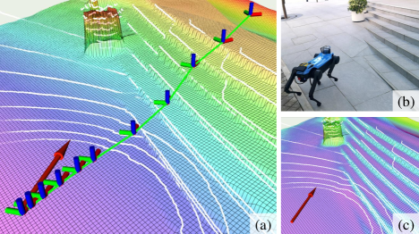
Figure 1: We present an online neural dense elevation mapping approach that recovers detailed urban terrain structures from sparse and noisy $16$-channel LiDAR observations (a)(b), while additionally providing the terrain reconstruction uncertainty (c). The framework can further benefit the downstream locomotion and navigation tasks, especially for legged robots.

To solve these issues, some approaches improve the mapping results based on the prior knowledge of terrain features, especially in urban environments [2, 3, 6, 1]. Due to the strong features recovery capabilities, Generative Adversarial Networks (GANs) are adopted for image inpainting [7, 8, 9] and 2D occupancy map completion [10, 11]. While image inpainting tasks focus more on visual rationality, directly using the generated maps in robotic applications may cause danger due to the absence of solid observations in the occluded regions. Therefore, providing the map reconstruction uncertainty is essential for the robust performance of the downstream tasks.

We present a neural urban terrain reconstruction framework for online end-to-end elevation mapping with measurable uncertainties using sparse LiDAR observations (Fig. 1). We design a novel approach to pre-process the point cloud frames. It maintains a group of statistical point features to represent the height distribution of points at each cell, enabling robust and efficient integration of new and history point frames. A Bayesian-GAN model is trained to generate dense elevation maps with minute details from the noisy and sparse point features based on the prior knowledge of urban terrain structures. The model additionally provides the reconstruction uncertainty for each grid, which can further improve the robustness of various downstream tasks. Compared with the state-of-the-art approaches [6, 12, 1], our approach provides robust dense reconstruction results with minute terrain details and uncertainty estimations while introducing less computational burden. Our main contributions include:

• We propose a novel framework for robust online neural terrain reconstruction to generate dense elevation maps from noisy and sparse LiDAR observations.

• We design a novel points pre-processing approach to represent and maintain the point features with a high data utilization rate and computational efficiency.

• We develop a Bayesian-GAN model that recovers the urban terrain structures with minute details and provides the pixel-wise reconstruction uncertainty.

• We conduct extensive experiments on our approach for high-quality terrain mapping with real-time performance on an AGX Xavier, demonstrating its benefits to downstream robotic tasks.

II Related Work

II-A Scene Representation Requirements in Downstream Tasks

Robotic applications adopt various terrain representation approaches to fulfill their requirements in specific scenarios. Existing approaches perform global path planning on meshes [13, 14, 15], Signed Distance Fields (SDFs) [16, 17, 18], and Neural Radiance Fields (NeRFs) [19, 20]. To achieve online local path planning in complex 3D scenarios, Frey et al. [21] use occupancy voxels to build volumetric traversability maps for quadrupedal robots. However, generating high-resolution voxels for detailed scene representation still brings a heavy burden to onboard devices. As legged robots concern more about the ground conditions, elevation maps are more widely adopted in their applications with online mapping requirements including motion planning [22, 23, 24, 25, 26] and navigation [27, 28, 29, 30, 31].

II-B 3D Scene Reconstruction Approaches

Extensive research has been conducted on 3D scene reconstruction in the past decades. Truncated Signed Distance Fields (TSDFs) are widely used for detailed structure representation, which can be further transformed into Euclidean Signed Distance Fields (ESDFs) as proposed in Voxblox [32] or VDBFusion [33] for navigation. NeRFs are constructed using multi-view images [34, 35, 36] and adopted to represent large-scale urban environments [2, 3]. However, they normally require intensive observation for better performance and introduce a high computation burden to mobile devices. This limits their applications with online local mapping requirements such as locomotion, local path planning, and exploration.

Some approaches describe the volumetric occupancy or terrain height to simplify the calculation. Hornung et al. [37] propose OctoMap for probabilistic 3D occupancy estimation. Jia et al. [38] develop an accelerator for real-time OctoMap building on embedded platforms. Stepanas et al. [39] adopt GPU for online occupancy map generation. As mentioned before, elevation maps are widely used as more efficient representations of terrain features. Fankhauser et al. [4, 5] present a robot-centric probabilistic elevation mapping approach that also returns the mapping uncertainty. Miki et al. [6] implement a GPU pipeline for efficient elevation mapping while supporting various post-processing functions. However, these approaches normally fail to recover dense and detailed terrain features due to occlusions and the inaccuracy of sensors and pose estimations. Our approach provides online neural dense elevation mapping with uncertainty estimations. Different from the uncertainty in [4, 5], our approach additionally considers the uncertainty from map completion, which leads to a more robust performance of downstream tasks.

II-C Scene Completion and Map Inpainting

Various map inpainting and scene completion methods leverage data-driven approaches or the prior information of terrain structure to solve the occlusion problem and optimize the reconstruction results. Existing works use learning-based approaches for 2D occupancy maps inpainting [40, 11], or for 3D semantic scene completion [41, 42]. Hoeller et al. [1] implement an online scene reconstruction method to generate occupancy voxels for structured terrains using a neural network.

Some recent work introduces real-time elevation map inpainting approaches. Given a raw elevation map, Miki et al. [6] apply inpainting filters and perform plane segmentation to recover the empty grids and extract geometric surfaces from the noisy map. Stölzle et al. [12] recover the occluded region on the raw map using a neural network. We present an end-to-end framework that efficiently pre-processes the sparse LiDAR observations to obtain the point features and then adopts a Bayesian-GAN model for real-time local dense elevation mapping. By using the robust point features representation approach and leveraging the strong generation capabilities of the proposed model, our approach maintains better details of complex terrain structures than [26] and [12].

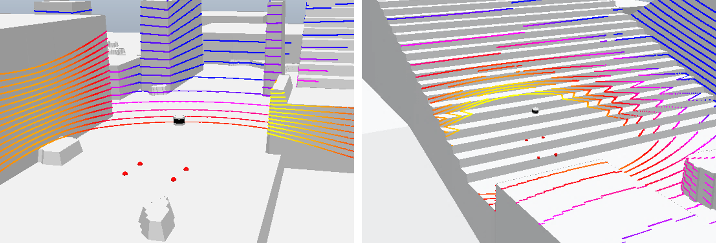
Figure 2: Examples of the simulation environment for dataset collection. The generated maps contain diverse types of urban terrains. A LiDAR with 16 channels is simulated to observe the environment, whose pose changes with the local topography considering the robot’s foot configuration (red balls).

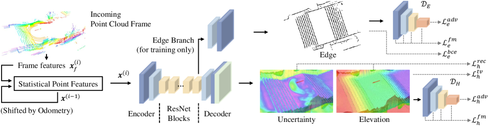
Figure 3: The proposed elevation mapping pipeline. It first pre-processes the observed sparse point clouds to update the maintained statistical point features. A Bayesian-GAN model then encodes the current point features to generate the elevation map and the pixel-wise reconstruction uncertainty while simultaneously returning a binary edge map for multitask learning in the training phase. Two discriminators are adopted to guide the learning of elevation map and edge map generation using adversarial loss $\mathcal{L}^{adv}$ and feature matching loss $\mathcal{L}^{fm}$.

III Approach

This section explains our problem formulation and illustrates how we design the dataset generation environment, data pre-processing approach, network architecture, and training objectives in detail.

III-A Problem Formulation

We focus on an online mapping scenario, where the robot continuously observes the surrounding static environment during its motion and receives sparse 3D point clouds from a LiDAR. The local terrain features are represented as robot-centric grid maps $\mathbf{y}_{h}$, where each grid cell on the 2D plane contains a height value of the corresponding location. Our elevation mapping process is to obtain dense maps of height estimations $\mathbf{\hat{y}}_{h}$ that recover the terrain features given the noisy and sparse observations $\mathbf{P}$ from sequential LiDAR frames and the robot motion estimates $\mathbf{e}$.

Generating dense elevation maps to represent detailed terrain features is a heavily ill-posed problem due to the observation inaccuracy and occlusions. Therefore, our approach specifically concerns the terrain reconstruction problem in urban environments, which holds the prior knowledge that the terrains are structured with sharp edges, flat surfaces, or smooth slopes. We take the advantage of the GAN models to learn the urban structures for terrain feature recovery and map generation. The point cloud frame $\mathbf{P}^{(i)}$ at time $i$ is processed to update the maintained point features $\mathbf{x}^{(i)}$ which is a multi-channel pseudo image containing the statistical features of the previous point clouds. Then a GAN-based inpainting model can be modified for dense map generation. The concept of Bayesian learning [43] is additionally introduced to measure the terrain reconstruction uncertainty for better training performance and more robust behaviors of the downstream tasks.

III-B Dataset Generation

To generate the dataset for training, we prepare multiple maps with various urban terrain features and simulate a $16$-channel LiDAR to observe the environment (Fig. 2). The maps contain regions of flat grounds, stairs, slopes, corridors, as well as irregular obstacles with various shapes and height values. The LiDAR is placed $0.50$m above the ground, which adopts the configuration of a Jueying Mini [44] quadrupedal robot (Fig. 1(b)). The ground truth height maps $\mathbf{y}_{h}$ are $5$m $\times$ $5$m patches with a resolution of $0.04$m centered around the position of the robot. We also generate the ground truth binary edge maps $\mathbf{y}_{e}$ using the Canny edge detector as done in [43] for multitask learning [45] which will be further explained in Section III-D.

The environment settings and observations are extensively augmented, which is essential to reduce the sim-to-real gap [1]. In each step, we move the LiDAR forward along a predefined trajectory around the global map center with a random linear velocity in $[0.0,1.0]$m/s. We also calculate the robot’s footprint positions according to the robot configuration and the local topography to obtain the corresponding LiDAR poses which are then slightly perturbed to simulate the body vibrations from locomotion. When a new point cloud is received, we add small random values in $[-0.02,0.02]$m on the coordinate of each point to mimic the sensory noise. The robot odometry in each step is also perturbed with random translations in $[-0.02,0.02]$m and rotations in $[-0.04,0.04]$rad to simulate the inaccuracy from pose estimation.

We define a grid cell inside the mapping region around the robot to be observed if at least one data point is found at that cell during the robot motion. Since the observations right after initialization are too sparse for a meaningful terrain reconstruction, we calculate the “observation rate” of a patch, which is the number of observed grids divided by the total number of grids in that patch, to filter out invalid data frames. The data frame will be dropped if the observation rate of the local patch is less than $25\%$. The final dataset contains $30$k valid data with an average observation rate of $60\%$.

III-C Point Features Representation

Due to the sparsity of LiDAR observations, it is difficult to recover detailed terrain structures from single LiDAR frames. One trivial solution is to use a buffer that replaces the old point cloud with the new frame and processes all the frames inside to obtain the network input in each step. However, this approach drops the history data to save memory and repeatedly processes a large number of points, which results in a low data utilization rate and computation efficiency. Hoeller et.al [1] adopts a recurrent structure to continuously refine the previous reconstruction results. Nevertheless, this approach may introduce the potential risk of accumulating the network reconstruction errors.

We design a robust data pre-processing approach that represents the distributions of the point height values in individual grids as they reflect the terrain structures. For example, the height values of points on the flat ground gather around the height of the surface, which approximately follows a Gaussian distribution. While on a vertical surface, the points may distribute uniformly from the upper to the lower boundary of the edge. In this case, we adopt Gaussian models to represent the point distribution properties and calculate the statistical features (denoted in upper case) for points in each grid as the network input. The maintained point features $\mathbf{x}^{(i)}$ for individual grids at time $i$ contains the number of points $C^{(i)}$, the mean and variance of observed height values $E^{(i)}(Z)$ and $Var^{(i)}(Z)$, as well as the mean and variance of the maximum and the minimum height overtime $E^{(i)}(Z_{max})$, $Var^{(i)}(Z_{max})$ and $E^{(i)}(Z_{min})$, $Var^{(i)}(Z_{min})$.

When we receive a new point cloud frame $\mathbf{P}^{(i+1)}$, we first rasterize the points inside the local mapping region and extract features (in lower case) for this single frame. The frame features $\mathbf{x}_{f}^{(i)}$ contain the number of points $c^{(i+1)}$, the sum of height values $\sum z^{(i+1)}$, the sum of the squared height values $\sum(z^{2})^{(i+1)}$, as well as the maximum and minimum height values $z_{max}^{(i+1)}$ and $z_{min}^{(i+1)}$ of each grid. The empty grids are filled with zeros. Next, the maintained point features $\mathbf{x}^{(i)}$ are transformed to be aligned with the current body position and can be easily updated using the frame features $\mathbf{x}_{f}^{(i)}$ based on the relationship $Var(z)=E(z^{2})-E^{2}(z)$. For instance, to update the mean of the height values:

$$C^{(i+1)}=C^{(i)}+c^{(i+1)},$$ (1)

$$E^{(i+1)}(Z)=\frac{C^{(i)}\times E^{(i)}(Z)+\sum z^{(i+1)}}{C^{(i+1)}},$$ (2)

and the variance:

$$E^{(i)}(Z^{2})=Var^{(i)}(Z)+(E^{2})^{(i)}(Z),$$ (3)

$$\sum(Z^{2})^{(i+1)}=C^{(i)}\times E^{(i)}(Z^{2})+\sum(z^{2})^{(i+1)},$$ (4)

$$Var^{(i+1)}(Z)=\frac{\sum(Z^{2})^{(i+1)}}{C^{(i+1)}}-(E^{2})^{(i+1)}(Z).$$ (5)

The mean and the variance values of $Z_{max}$ and $Z_{min}$ are obtained in the same way.

Our approach only pre-processes a single LiDAR frame in each step and the maintained point features are updated with simple rules. This achieves high memory and computational efficiency on mobile devices. Although combining multiple LiDAR frames suffers from sensory noise and odometry inaccuracy, the maintained point distributions will converge to stable states as the number of observations increases assuming that the odometry drifts in an acceptable range in a local mapping scenario. This also improves the stability of neural map generation. One side effect is that the influence of new frames will gradually decrease as the number of points accumulates. Therefore, we append a final step of the update that decays the point count $C^{(i+1)}$ of a grid with a factor $\gamma$ and limits the number of points with $C_{max}$ if there are new points observed at that grid:

$$C^{(i+1)}=\min(C_{max},\ \gamma C^{(i)}+c^{(i+1)}),$$ (6)

where we set the maximum point count $C_{max}=100$ and $\gamma=0.90$ to encourage the updates using new data frames.

III-D Network Architecture

One of the major objectives in our network design is to recover the detailed terrain structures with high-quality edges because edges contain important terrain features that are quite essential to improve the safety and efficiency of downstream tasks. As explained in [7], traditional image inpainting pipelines suffer from blurry or artifacts due to the difficulties in recovering the high-frequency component. In this case, they present EdgeConnect which sequentially adopts an edge generator and an image completion network to separately conquer the edge recovery and image inpainting. We reference the architecture of EdgeConnect while adopting multitask learning [45] for simultaneous edge generation and elevation mapping. This assists the model to maintain high-frequency components in the bottleneck features while achieving higher inference speed compared with the serial structure of EdgeConnect.

Fig. 3 presents the pipeline and network architecture of our approach. The maintained point features $\mathbf{x}^{(i)}$ are first passed into convolutional layers for encoding, which are then down-sampled before entering six ResNet blocks for feature extraction. Each ResNet block contains a dilated convolutional layer for larger receptive fields and a normal convolutional layer for output. Two decoding blocks respectively up-sample the bottleneck features and generate the binary edges $\mathbf{\hat{y}}_{e}$ and height maps $\mathbf{\hat{y}}_{h}$. Based on the concept of Bayesian learning, the height map generation block also returns a log scale variance map $\log\boldsymbol{\sigma}$ as the reconstruction uncertainty, which is integrated into the reconstruction loss in Section III-E and jointly optimized with the height map. Two discriminators with convolutional layers $\mathcal{D}_{E}$ and $\mathcal{D}_{H}$ are implemented to guide the training of edge and height map generation. During deployment, only the height map branch in the generator is activated for fast inference. Because the network is fully convolutional, it can deal with different input sizes to adapt to the mapping requirements of various downstream tasks.

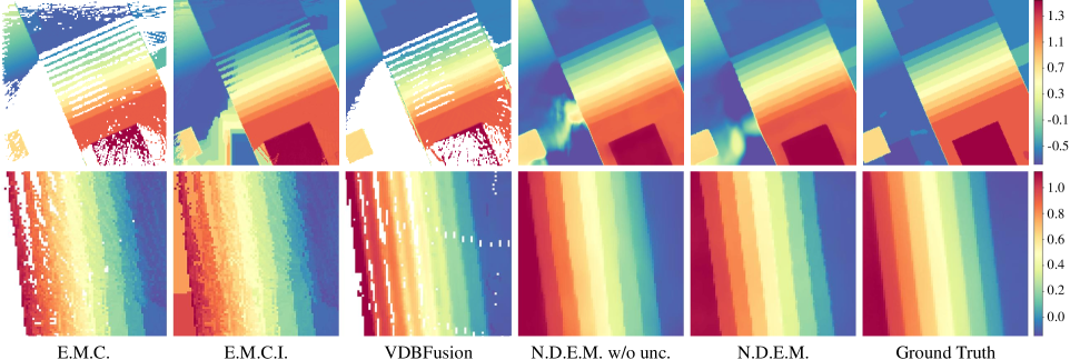
Figure 4: Visualized examples of the elevation mapping experiments in simulations (the first row, $8$m $\times$ $8$m) and on real-world stairs (the second row, $3.2$m $\times$ $3.2$m) using different approaches, where different colors indicate the height of steps. Our approach (N.D.E.M.) provides accurate dense elevation maps with high reconstruction quality and can recover detailed terrain structures even under noisy and sparse observations.

III-E Training Objectives

During the training process, the edge generation is optimized using a pixel-wise binary cross-entropy loss $\mathcal{L}_{e}^{bce}$ that is clipped afterward for numerical stability:

$$\mathcal{L}_{e}^{bce}=-\sum\left(\mathbf{y}_{e}\log\mathbf{\hat{y}}_{e}+(1-\mathbf{y}_{e})\log(1-\mathbf{\hat{y}}_{e})\right).$$ (7)

For height map generation, we use the heteroscedastic model in [43] to formulate our reconstruction loss $\mathcal{L}_{h}^{rec}$ and measure the data-dependent reconstruction uncertainty, where L1 norm is adopted due to its robustness to outlying residuals:

$$\mathcal{L}_{h}^{rec}=\sum\frac{\sqrt{2}}{\boldsymbol{\sigma}}||\mathbf{y}_{h}-\mathbf{\hat{y}}_{h}||+\log\boldsymbol{\sigma}.$$ (8)

Provided the prior information on structured urban terrains, we introduce the unsupervised total variant loss $\mathcal{L}_{h}^{tv}$ to obtain smooth planes and sharp edges in the generated height maps:

$$\mathcal{L}_{h}^{tv}=\sum\sum_{j,k}|\hat{y}_{(h)\,j+1,k}-\hat{y}_{(h)\,j,k}|+|\hat{y}_{(h)\,j,k+1}-\hat{y}_{(h)\,j,k}|,$$ (9)

where $j$, $k$ are map indices in rows and columns.

Both the edge and the height map generation additionally adopt the adversarial loss $\mathcal{L}^{adv}$ and the feature matching loss $\mathcal{L}^{fm}$ calculated from the respective discriminators. The generation adversarial loss is defined as:

$$\mathcal{L}^{adv}=\sum\log(1-\mathcal{D}(\mathbf{\hat{y}})).$$ (10)

Similar to [7], the feature matching loss is calculated by comparing the feature maps from multiple intermediate convolutional blocks $\mathcal{D}^{(l)}$ in the discriminators:

$$\mathcal{L}^{fm}=\sum||\mathcal{D}^{(l)}(\mathbf{y})-\mathcal{D}^{(l)}(\mathbf{\hat{y}})||.$$ (11)

The overall optimization objective of the generation model is the weighted sum of all the above terms, where the generated edge $\mathbf{\hat{y}}_{e}$, height map $\mathbf{\hat{y}}_{h}$, and log variance $\log\boldsymbol{\sigma}$ are jointly optimized:

$$\mathcal{L}^{total}=\mathbf{w}^{T}[\mathcal{L}^{bce}_{e},\mathcal{L}^{adv}_{e},\mathcal{L}^{fm}_{e},\mathcal{L}^{rec}_{h},\mathcal{L}^{tv}_{h},\mathcal{L}^{adv}_{h},\mathcal{L}^{fm}_{h}]^{T}.$$ (12)

IV Experiments

IV-A Implementation Details

IV-A1 Setup

We adopt CoppeliaSim [46] to build our environment and collect dataset for training and evaluation. In simulation experiments, we generate maps as in Fig. 2 containing various terrain features to collect an evaluation dataset containing around $2$k data frames using the same approach as illustrated in Section III-B. All the mapping approaches are evaluated using $5$m $\times$ $5$m patches.

For real-world experiments, we specifically focus on the mapping performance on stairs as it is one of the most challenging terrain reconstruction scenarios containing detailed structures, which is frequently used for mapping evaluation in [1, 6, 12], and the reconstruction quality of stairs can largely affect the downstream tasks. We control a Jueying Mini [44] quadrupedal robot to approach or walk up multiple stairs with various heights and steepness. The robot receives sparse point clouds at $10$Hz from a RoboSense RS-LiDAR-16 as the observation of the environment. The odometry information of the robot is obtained using a modified version of Normal Distribution Transform (NDT) [47] which continuously compare the current LiDAR frame with a local point cloud map containing $5$ nearest frames. All the mapping approaches are evaluated using $2$m $\times$ $2$m patches on stairs, where the same network model of our approach is used as in the simulation experiments.

To obtain the ground truth maps in the real world, we collect dense point clouds using multiple point frames from an Ouster OS1 LiDAR with 128 channels. The poses of these frames are globally optimized using FAST-LIO [48]. Next, we adopt VDBFusion [33] which performs well with dense input and accurate odometry information to reconstruct the terrain structures. We finally rasterize the results as the ground truth height maps. In each experiment, the relative transformation between the ground truth and the generated map origin is obtained by performing ICP on the initial sparse observation frame and the dense point cloud.

IV-A2 Baseline approaches

We compare the mapping performance of our approach (denoted as N.D.E.M.) with the CuPy implementation of elevation mapping [6] which provides the raw elevation maps (E.M.C.) and the results after an inpainting filter (E.M.C.I.). We also adopt VDBFusion to incrementally reconstruct the terrain using incoming sparse observations and rasterize the results for comparison. To show the improvement of introducing the uncertainty estimation, we additionally train a model without using Bayesian learning (N.D.E.M. w/o unc.).

IV-A3 Evaluation metrics

The mean absolute error (MAE) is widely adopted to measure the accuracy of pixel values. In addition, we introduce the mean gradient difference (MGD) which is the averaged L2 norm of the gradient differences between the ground truths and the generation results to measure the capability of maintaining minute details at flat surfaces and edges. As it is not quite meaningful to consider the accuracy of grids in a heavily occluded region, we mask a grid if the observation rate of a $1$m $\times$ $1$m patch around it is less than $50\%$ and obtain the masked results (mMAE and mMGD) to measure the reconstruction accuracy. We also calculate the peak signal-to-noise ratio (PSNR) and structural similarity index measure (SSIM) without applying the masks to further evaluate the noise level and visual similarity. For the approaches without a guarantee on dense mapping (E.M.C. and VDBFusion), we use bilinear interpolation on their results to fill in the empty region for calculation.

IV-B Simulation Results

Table I presents the mapping performance in the simulation experiments. Our approach achieves the highest mapping accuracy in height values and their gradients. Despite the sensory noises and odometry drifts in the observations, our approach can still recognize the terrain structure and generate high-quality maps. The high structural similarity also indicates the effectiveness of our GAN model in generating rational urban structures. By introducing Bayesian learning that integrates the uncertainty estimations in the reconstruction loss, our model (N.D.E.M.) achieves better learning performance (compared with N.D.E.M. w/o unc.).

TABLE I: Elevation Mapping Performance in Simulation

	mMAE $\downarrow$	mMGD $\downarrow$	PSNR $\uparrow$	SSIM $\uparrow$
E.M.C.	3.4350	0.7415	48.62	0.5619
E.M.C.I.	2.5650	0.5446	61.13	0.7441
VDBFusion	3.3989	0.6590	53.85	0.6303
N.D.E.M. w/o unc.	3.4329	0.4071	62.91	0.7259
N.D.E.M.	2.3327	0.3417	66.15	0.8005

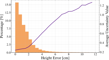
Figure 5: The percentage (orange bar plot) of different levels of error and the corresponding uncertainty (purple curve). Our approach provides high-quality mapping results that are accurate enough for various downstream tasks. The uncertainty estimations further reflect the confidence of our model on the generated maps.

To intuitively evaluate the accuracy of our approach on map generation and uncertainty estimations, we plot the percentage of different height error levels in simulations and the corresponding averaged uncertainty values $\boldsymbol{\sigma}$. The histogram in Fig. 5 shows the percentage of mMAE values among all the simulation results, which indicates that more than three-quarters of the grids have an error of less than $2$cm, and around half of the grids achieve an even higher accuracy ($<1$cm). The curve in Fig. 5 plots the change of uncertainty over the unmasked errors considering all the generated height values. It shows that the uncertainty values are close to being linearly proportional to the errors, which successfully reflects the confidence of our model on mapping results. The first row of Fig. 4 visualizes an example of the mapping results in simulation, where we use $8$m $\times$ $8$m patches containing multiple urban terrain features for qualitative evaluation. Our approach provides high-quality dense elevation maps in this complex scenario with detailed features of various kinds of terrains.

IV-C Real-world Performance

Table II shows the mapping performance on real-world stairs. Our approach still performs well with high accuracy while maintaining detailed terrain structures and high structural similarity. The filtering-based inpainting approach (E.M.C.I.) presents a worse performance than in simulation, probably because the robot travels longer linear distances in the real-world scenarios without looping back, which results in lower observation rates and the filter-based approach requires enough observations for satisfactory results. The VDBFusion has an acceptable performance at the expense of memory and computational efficiency as it incrementally constructs a global map, which may introduce a heavy burden to the mobile device.

TABLE II: Elevation Mapping Performance on Real-world Stairs

	mMAE $\downarrow$	mMGD $\downarrow$	PSNR $\uparrow$	SSIM $\uparrow$
E.M.C.	4.2591	0.7090	73.32	0.7657
E.M.C.I.	4.1782	0.7364	72.77	0.7526
VDBFusion	3.5930	0.5455	74.98	0.8186
N.D.E.M. w/o unc.	2.8889	0.4222	76.16	0.8678
N.D.E.M.	2.3868	0.3858	77.48	0.8889

We further visualize an example of the mapping results in a real-world scenario on a stair. As shown in the second row of Fig. 4, the traditional elevation mapping approach (E.M.C.) is quite sensitive to noises and the occluded regions are invalid. Although the inpainting filter assists to provide dense mapping results, it fails to recover the map structures from noises and the inpainting is inaccurate if there is not enough observation. The VDBFusion successfully reconstruct the stair structures for the first several steps. However, it still cannot provide dense results and the performance is unsatisfactory for the former steps. Our approach provides high-quality dense mapping results with minute stair structures, while the version with uncertainty estimations further improves the sharpness of edges.

IV-D Benefits to Downstream Tasks

We deploy a Python implementation of the proposed elevation mapping framework on an Nvidia Jetson AGX Xavier. The point cloud pre-processing and point features update are accelerated using GPU through CuPy element-wise kernels. It takes only around $1.2$ms to preprocess a point cloud frame from a LiDAR with $16$ channels and generate the network input. As the generation model is fully convolutional, it can deal with input feature maps of diverse sizes and generate maps of the corresponding shape. The model takes around $24$ms to generate $3.2$m $\times$ $3.2$m local patches for locomotion as done in [1] and uses $75$ms to generate $12$m $\times$ $12$m maps for cost-optimal navigation on complex terrains as required in [28]. The whole pipeline performs elevation mapping at $10$Hz, which achieves real-time performance on the mobile computation platform and saves computational resources for other robotic tasks.

We then conduct path planning on real-world stairs using the approach in [28] which requires dense elevation maps for optimal path planning on complex terrains. As shown in Fig. 6, both E.M.C.I. and our approach provide online dense elevation mapping when the robot approaches the stair. However, E.M.C.I. cannot recover detailed stair structures from extremely sparse observations, resulting in the failure of the planner to find a valid path. Our approach successfully reconstructs the stair once the LiDAR observes the steps. The strong capability of our approach in reconstructing urban terrain features at a glance assists the navigation and exploration tasks to achieve better performance.

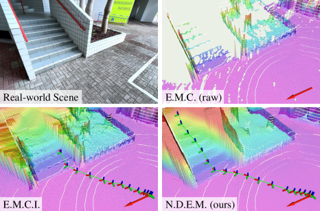
Figure 6: Our approach successfully recovers the structure of the real-world stair at a glance, presenting strong capabilities in urban terrain reconstruction with extremely sparse observation, which benefits various navigation and exploration applications.

Adopting the uncertainty estimations in the downstream tasks can help to ensure the safe and robust behaviors of the robot. Fig. 1(c) visualizes the uncertainty values on the real-world stairs. Our model returns a higher uncertainty at the edges of the stairs than the flat surfaces, which can assist the locomotion algorithms to step feet onto safe regions and prevent slips resulting from the terrain reconstruction inaccuracy. In addition, when there is a hole on the ground (Fig. 7), the inpainting filter (E.M.C.I.) [6] just fills in that region to make it a surface, resulting in potential danger to navigation tasks. Although our approach cannot provide accurate height values inside the hole due to occlusion, it returns high reconstruction uncertainty that can inform the navigation module for safe behaviors.

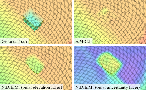
Figure 7: When there is a hole on the ground, rather than just fill in the hole as done by the filtering-based approach, our mapping module returns high uncertainty at the occluded region, informing the downstream tasks of the potential danger.

V Conclusion

We propose a learning-based dense elevation mapping framework for urban terrain reconstruction. It maintains high reconstruction quality and accuracy in both simulation and real-world scenarios. A GAN model is adopted to recognize and generate the terrain features in the occluded regions based on the prior knowledge of urban terrain. The proposed data pre-processing method and the map generation model show robust performance that can recover detailed terrain structures from sparse and noisy LiDAR observations, while also achieving high efficiency that can perform elevation mapping on mobile devices in real-time. By introducing the concept of Bayesian learning, the accuracy and generation quality of our model are further improved. The provided uncertainty estimations also have the potential to assist the downstream tasks for safer and more robust performance.

References

- [1] D. Hoeller, N. Rudin, C. Choy, A. Anandkumar, and M. Hutter, “Neural scene representation for locomotion on structured terrain,” IEEE Robotics and Automation Letters, vol. 7, no. 4, pp. 8667–8674, 2022.
- [2] K. Rematas, A. Liu, P. P. Srinivasan, J. T. Barron, A. Tagliasacchi, T. Funkhouser, and V. Ferrari, “Urban radiance fields,” in Proceedings of the IEEE/CVF Conference on Computer Vision and Pattern Recognition (CVPR), pp. 12932–12942, June 2022.
- [3] H. Guo, S. Peng, H. Lin, Q. Wang, G. Zhang, H. Bao, and X. Zhou, “Neural 3d scene reconstruction with the manhattan-world assumption,” in Proceedings of the IEEE/CVF Conference on Computer Vision and Pattern Recognition (CVPR), pp. 5511–5520, 2022.
- [4] P. Fankhauser, M. Bloesch, C. Gehring, M. Hutter, and R. Siegwart, “Robot-centric elevation mapping with uncertainty estimates,” in International Conference on Climbing and Walking Robots (CLAWAR), 2014.
- [5] P. Fankhauser, M. Bloesch, and M. Hutter, “Probabilistic terrain mapping for mobile robots with uncertain localization,” IEEE Robotics and Automation Letters, vol. 3, no. 4, pp. 3019–3026, 2018.
- [6] T. Miki, L. Wellhausen, R. Grandia, F. Jenelten, T. Homberger, and M. Hutter, “Elevation mapping for locomotion and navigation using gpu,” arXiv preprint arXiv:2204.12876, 2022.
- [7] K. Nazeri, E. Ng, T. Joseph, F. Qureshi, and M. Ebrahimi, “Edgeconnect: Structure guided image inpainting using edge prediction,” in Proceedings of the IEEE/CVF International Conference on Computer Vision (ICCV) Workshops, Oct 2019.
- [8] H. Liu, Z. Wan, W. Huang, Y. Song, X. Han, and J. Liao, “Pd-gan: Probabilistic diverse gan for image inpainting,” in Proceedings of the IEEE/CVF Conference on Computer Vision and Pattern Recognition (CVPR), pp. 9371–9381, June 2021.
- [9] W. Wang, L. Niu, J. Zhang, X. Yang, and L. Zhang, “Dual-path image inpainting with auxiliary gan inversion,” in Proceedings of the IEEE/CVF Conference on Computer Vision and Pattern Recognition (CVPR), pp. 11421–11430, June 2022.
- [10] K. Katyal, K. Popek, C. Paxton, J. Moore, K. Wolfe, P. Burlina, and G. D. Hager, “Occupancy map prediction using generative and fully convolutional networks for vehicle navigation,” arXiv preprint arXiv:1803.02007, 2018.
- [11] V. D. Sharma, J. Chen, A. Shrivastava, and P. Tokekar, “Occupancy map prediction for improved indoor robot navigation,” arXiv preprint arXiv:2203.04177, 2022.
- [12] M. Stölzle, T. Miki, L. Gerdes, M. Azkarate, and M. Hutter, “Reconstructing occluded elevation information in terrain maps with self-supervised learning,” IEEE Robotics and Automation Letters, vol. 7, no. 2, pp. 1697–1704, 2022.
- [13] D. S. Yershov and E. Frazzoli, “Asymptotically optimal feedback planning using a numerical hamilton-jacobi-bellman solver and an adaptive mesh refinement,” The International Journal of Robotics Research, vol. 35, no. 5, pp. 565–584, 2016.
- [14] S. Bhattacharya, “Towards optimal path computation in a simplicial complex,” The International Journal of Robotics Research, vol. 38, no. 8, pp. 981–1009, 2019.
- [15] S. Pütz, T. Wiemann, M. K. Piening, and J. Hertzberg, “Continuous shortest path vector field navigation on 3d triangular meshes for mobile robots,” in 2021 IEEE International Conference on Robotics and Automation (ICRA), pp. 2256–2263, IEEE, 2021.
- [16] H. Oleynikova, A. Millane, Z. Taylor, E. Galceran, J. Nieto, and R. Siegwart, “Signed distance fields: A natural representation for both mapping and planning,” in RSS 2016 workshop: geometry and beyond-representations, physics, and scene understanding for robotics, University of Michigan, 2016.
- [17] L. Gasser, A. Millane, V. Reijgwart, R. Bähnemann, and R. Siegwart, “Voxplan: A 3d global planner using signed distance function submaps,” in 2021 IEEE International Conference on Robotics and Automation (ICRA), pp. 7901–7907, IEEE, 2021.
- [18] Y. Wang, X. Zhang, Y. Liu, and Y. Zhuang, “2d topological map building by uavs for ground robot navigation,” in 2021 IEEE International Conference on Robotics and Biomimetics (ROBIO), pp. 663–668, IEEE, 2021.
- [19] M. Adamkiewicz, T. Chen, A. Caccavale, R. Gardner, P. Culbertson, J. Bohg, and M. Schwager, “Vision-only robot navigation in a neural radiance world,” IEEE Robotics and Automation Letters, vol. 7, no. 2, pp. 4606–4613, 2022.
- [20] M. Pantic, C. Cadena, R. Siegwart, and L. Ott, “Sampling-free obstacle gradients and reactive planning in neural radiance fields (nerf),” arXiv preprint arXiv:2205.01389, 2022.
- [21] J. Frey, D. Hoeller, S. Khattak, and M. Hutter, “Locomotion policy guided traversability learning using volumetric representations of complex environments,” arXiv preprint arXiv:2203.15854, 2022.
- [22] P. Fankhauser, M. Bjelonic, C. D. Bellicoso, T. Miki, and M. Hutter, “Robust rough-terrain locomotion with a quadrupedal robot,” in 2018 IEEE International Conference on Robotics and Automation (ICRA), pp. 5761–5768, IEEE, 2018.
- [23] C. Mastalli, I. Havoutis, M. Focchi, D. G. Caldwell, and C. Semini, “Motion planning for quadrupedal locomotion: Coupled planning, terrain mapping, and whole-body control,” IEEE Transactions on Robotics, vol. 36, no. 6, pp. 1635–1648, 2020.
- [24] F. Jenelten, T. Miki, A. E. Vijayan, M. Bjelonic, and M. Hutter, “Perceptive locomotion in rough terrain–online foothold optimization,” IEEE Robotics and Automation Letters, vol. 5, no. 4, pp. 5370–5376, 2020.
- [25] T. Miki, J. Lee, J. Hwangbo, L. Wellhausen, V. Koltun, and M. Hutter, “Learning robust perceptive locomotion for quadrupedal robots in the wild,” Science Robotics, vol. 7, no. 62, p. eabk2822, 2022.
- [26] F. Jenelten, R. Grandia, F. Farshidian, and M. Hutter, “Tamols: Terrain-aware motion optimization for legged systems,” IEEE Transactions on Robotics, pp. 1–19, 2022.
- [27] J. Guzzi, R. O. Chavez-Garcia, M. Nava, L. M. Gambardella, and A. Giusti, “Path planning with local motion estimations,” IEEE Robotics and Automation Letters, vol. 5, no. 2, pp. 2586–2593, 2020.
- [28] B. Yang, L. Wellhausen, T. Miki, M. Liu, and M. Hutter, “Real-time optimal navigation planning using learned motion costs,” in 2021 IEEE International Conference on Robotics and Automation (ICRA), pp. 9283–9289, IEEE, 2021.
- [29] L. Wellhausen and M. Hutter, “Rough terrain navigation for legged robots using reachability planning and template learning,” in 2021 IEEE/RSJ International Conference on Intelligent Robots and Systems (IROS), pp. 6914–6921, IEEE, 2021.
- [30] H. Hu, K. Zhang, A. H. Tan, M. Ruan, C. Agia, and G. Nejat, “A sim-to-real pipeline for deep reinforcement learning for autonomous robot navigation in cluttered rough terrain,” IEEE Robotics and Automation Letters, vol. 6, no. 4, pp. 6569–6576, 2021.
- [31] M. Mattamala, N. Chebrolu, and M. Fallon, “An efficient locally reactive controller for safe navigation in visual teach and repeat missions,” IEEE Robotics and Automation Letters, vol. 7, no. 2, pp. 2353–2360, 2022.
- [32] H. Oleynikova, Z. Taylor, M. Fehr, R. Siegwart, and J. Nieto, “Voxblox: Incremental 3d euclidean signed distance fields for on-board mav planning,” in 2017 IEEE/RSJ International Conference on Intelligent Robots and Systems (IROS), pp. 1366–1373, IEEE, 2017.
- [33] I. Vizzo, T. Guadagnino, J. Behley, and C. Stachniss, “Vdbfusion: Flexible and efficient tsdf integration of range sensor data,” Sensors, vol. 22, no. 3, p. 1296, 2022.
- [34] B. Mildenhall, P. P. Srinivasan, M. Tancik, J. T. Barron, R. Ramamoorthi, and R. Ng, “Nerf: Representing scenes as neural radiance fields for view synthesis,” in European conference on computer vision, pp. 405–421, Springer, 2020.
- [35] T. Chen, P. Wang, Z. Fan, and Z. Wang, “Aug-nerf: Training stronger neural radiance fields with triple-level physically-grounded augmentations,” in Proceedings of the IEEE/CVF Conference on Computer Vision and Pattern Recognition (CVPR), pp. 15191–15202, June 2022.
- [36] M. Tancik, V. Casser, X. Yan, S. Pradhan, B. Mildenhall, P. P. Srinivasan, J. T. Barron, and H. Kretzschmar, “Block-nerf: Scalable large scene neural view synthesis,” in Proceedings of the IEEE/CVF Conference on Computer Vision and Pattern Recognition (CVPR), pp. 8248–8258, June 2022.
- [37] A. Hornung, K. M. Wurm, M. Bennewitz, C. Stachniss, and W. Burgard, “Octomap: An efficient probabilistic 3d mapping framework based on octrees,” Autonomous robots, vol. 34, no. 3, pp. 189–206, 2013.
- [38] T. Jia, E.-Y. Yang, Y.-S. Hsiao, J. Cruz, D. Brooks, G.-Y. Wei, and V. J. Reddi, “Omu: A probabilistic 3d occupancy mapping accelerator for real-time octomap at the edge,” in 2022 Design, Automation & Test in Europe Conference & Exhibition (DATE), pp. 909–914, 2022.
- [39] K. Stepanas, J. Williams, E. Hernández, F. Ruetz, and T. Hines, “Ohm: Gpu based occupancy map generation,” arXiv preprint arXiv:2206.06079, 2022.
- [40] M. Wei, D. Lee, V. Isler, and D. Lee, “Occupancy map inpainting for online robot navigation,” in 2021 IEEE International Conference on Robotics and Automation (ICRA), pp. 8551–8557, IEEE, 2021.
- [41] S. Song, F. Yu, A. Zeng, A. X. Chang, M. Savva, and T. Funkhouser, “Semantic scene completion from a single depth image,” in 2017 IEEE Conference on Computer Vision and Pattern Recognition (CVPR), pp. 190–198, 2017.
- [42] J. Zhang, H. Zhao, A. Yao, Y. Chen, L. Zhang, and H. Liao, “Efficient semantic scene completion network with spatial group convolution,” in European Conference on Computer Vision, pp. 749–765, Springer, 2018.
- [43] A. Kendall, Geometry and uncertainty in deep learning for computer vision. PhD thesis, University of Cambridge, UK, 2019.
- [44] “Jueying Mini.” https://www.deeprobotics.cn/en/products_jy_301.html. Accessed: 2021-08-30.
- [45] R. Caruana, “Multitask learning,” Machine learning, vol. 28, no. 1, pp. 41–75, 1997.
- [46] E. Rohmer, S. P. N. Singh, and M. Freese, “Coppeliasim (formerly v-rep): a versatile and scalable robot simulation framework,” in Proc. of The International Conference on Intelligent Robots and Systems (IROS), 2013. www.coppeliarobotics.com.
- [47] M. Magnusson, The three-dimensional normal-distributions transform: an efficient representation for registration, surface analysis, and loop detection. PhD thesis, Örebro universitet, 2009.
- [48] W. Xu and F. Zhang, “Fast-lio: A fast, robust lidar-inertial odometry package by tightly-coupled iterated kalman filter,” IEEE Robotics and Automation Letters, vol. 6, no. 2, pp. 3317–3324, 2021.