Analysis of eight magnetic chemically peculiar stars with rotational modulation

Abstract

Since the end of 2018, the Transiting Exoplanet Survey Satellite (TESS) has provided stellar photometry to the astronomical community. We have used TESS data to study rotational modulation in the light curves of a sample of chemically peculiar stars with measured large-scale magnetic fields (mCP stars). In general, mCP stars show inhomogeneous distributions of elements in their atmospheres that lead to spectroscopic (line profile) and photometric (light curve) variations commensurate with the rotational period. We analyzed the available TESS data from 50 sectors for eight targets after post-processing them in order to minimize systematic instrumental trends. Analysis of the light curves allowed us to determine rotational periods for all eight of our targets. For each star, we provide a phase diagram calculated using the derived period from the light curves and from the available measurements of the disk-averaged longitudinal magnetic field $\langle B_{\rm z}\rangle$. In most cases, the phased light curve and $\langle B_{\rm z}\rangle$ measurements show consistent variability. Using our rotation periods, and global stellar parameters derived from fitting Balmer line profiles, and from Geneva and Strömgren-Crawford photometry, we determined the equatorial rotational velocities and calculated the respective critical rotational fractions $v_{\rm eq}/v_{\rm crit}$. We have shown from our sample that the critical rotational fraction decreases with stellar age, at a rate consistent with the magnetic braking observed in the larger population of mCP stars.

1 Introduction

Table 1: Stellar parameters collected from the literature and derived from our analysis of observed data for the ApBp stars studied in this work. Column (1) presents the HD number, column (2) shows the spectral type of each star inferred from recent studies. Columns (3), (4), (5), and (6) provide data for effective temperature and surface gravity collected from the TESS Input Catalog (TIC)¹ and derived from fitting the Balmer line profiles respectively. Column (7) and (8) present rotational periods extracted from the literature and derived from the analysis of light curves. Columns (9) and (10), and (11) and (12) show v$\sin{i}$ and radial velocity inferred from the literature and derived from fitting the Balmer line profiles, respectively.

Name	Spectral type	$T_{\rm eff}$ (K)		$\log{g}$		Period (d)		v$\sin{i}$ (km s-1)		vr (km s-1)
	SIMBAD	TIC1	This study	TIC1	This study	Published	This study	SIMBAD	This study	SIMBAD	This study
			Balmer		Balmer				Balmer		Balmer
HD10840	B92	11663$\pm$317	-	4.11$\pm$0.07	-	2.097679(7)6	2.0976858(2)	35.0$\pm$5.014	-	19.4$\pm$2.121	-
HD22920	B8II3	13800$\pm$200	13678$\pm$200	-	3.77$\pm$0.20	3.9472(1)7	3.947225(2)	37.0$\pm$5.015	33.0$\pm$5.0	18.0$\pm$4.015	18.0$\pm$3.0
HD24712	A9Vp4	7242$\pm$129	7290$\pm$200	4.18$\pm$0.08	4.06$\pm$0.20	12.461(1)8	12.45862(5)	6.6$\pm$0.616	9.0$\pm$3.0	23.2$\pm$0.422	22.0$\pm$2.0
HD38170	B95	10000$\pm$280	9470$\pm$200	3.80 $\pm$ 0.08	3.65$\pm$0.20	2.76618(4)9	2.766116(2)	65.0$\pm$9.017	65.0$\pm$3.0	36.3$\pm$0.622	33.0$\pm$2.0
HD63401	B95	-	13356$\pm$200	-	4.06$\pm$0.20	2.41(2)10	2.414474(1)	52.0$\pm$4.018	52.0$\pm$4.0	22.0$\pm$1.422	26.0$\pm$4.0
HD74521	A1Vp6	12188$\pm$146	10600$\pm$200	-	3.47$\pm$0.20	7.0501(2)11	7.05010(5)	19.0$\pm$4.619	18.0$\pm$3.0	27.5$\pm$1.422	24.0$\pm$3.0
HD77314	A25	9253$\pm$372	11437$\pm$200	3.69$\pm$0.10	3.99$\pm$0.20	2.86445(8)12	2.864325(1)	-	47.0$\pm$3.0	-	-4.0$\pm$1.0
HD86592	A05	8129 $\pm$145	7804$\pm$200	4.18$\pm$0.07	3.83$\pm$0.20	2.886713	2.88657(3)	16.2$\pm$2.020	27.0$\pm$5.0	12.7$\pm$0.320	13.0$\pm$1.0

Note: ¹Stassun et al. (2018, 2019), ²Renson & Manfroid (1992), ³Houk & Swift (1999), ⁴Abt & Morrell (1995), ⁵Cannon & Pickering (1993), ⁶Sikora et al. (2019c), ⁷Shultz et al. (2022), ⁸Bagnulo et al. (1995), ⁹David-Uraz et al. (2021), ¹⁰Hensberge et al. (1976), ¹¹Dukes & Adelman (2018), ¹²Bernhard et al. (2020), ¹³Babel & North (1997), ¹⁴Bailey & Landstreet (2013), ¹⁵Khalack & Poitras (2015), ¹⁶Sikora et al. (2019a), ¹⁷Royer et al. (2002), ¹⁸Bailey et al. (2014), ¹⁹Mathys (1995), ²⁰Babel & North (1997), ²¹Levato et al. (1996), ²²Gontcharov (2006)

Chemically peculiar (CP) stars on the upper main sequence (MS) are identified through abnormally strong absorption lines of some chemical elements. In particular ApBp stars, which were classified as CP2 by Preston (1974), are characterized by strong lines of metals such as Si, Cr, Fe, Sr, and rare earth elements. Such peculiarities that occur in stellar atmospheres might be the result of the competition between gravitational settling and radiative acceleration (Michaud, 1970), leading to a relative movement between the different ions of the plasma known as atomic diffusion (Alecian & Stift, 2010).

Preston (1974) mentioned that the group of magnetic ApBp stars shows relatively slow rotation compared to normal stars of A and B spectral types with the same effective temperatures. Magnetic fields detected in ApBp stars (e.g. Bychkov et al., 2003; Buysschaert et al., 2018; Shultz et al., 2022) are thought to have a fossil origin (Neiner et al., 2015) and are known to range in strength from a few hundred G up to a few tens of kG (Aurière et al., 2007; Shultz et al., 2019; Sikora et al., 2019b). The influence of magnetic fields in ApBp stars is quite significant. It prevents rotational mixing and therefore amplifies atomic diffusion (Alecian & Stift, 2010) producing an inhomogeneous redistribution of elements in stellar atmospheres. It is thought that the magnetic field stabilizes the stellar atmosphere, enabling diffusion to play a greater role as compared, for example, to Am stars (Michaud et al., 2015), which are generally not known to host strong, organized fields at their surface. The magnetic fields of most ApBp stars tend to be predominantly dipolar (Kochukhov et al., 2019).

In general, the rotational and magnetic dipole axes are not aligned in CP stars.To first order, the distribution of the abundance spots over the stellar surface is governed by the magnetic geometry (Alecian & Stift 2019, 2021). These spots result in flux redistribution which is translated to the appearance of brightness spots leading to the modulation of light curves by stellar rotation (Krtička et al., 2015). The description of abundance anomalies in ApBp stars is not an easy task considering that an element’s abundance shows both horizontal segregation and vertical stratification in their atmospheres (LeBlanc et al., 2015; Khalack et al., 2017; Khalack, 2018; Ndiaye et al., 2018; Khalack et al., 2020). The group of mCP stars exhibits variability of spectral line profiles (Krtička et al., 2015), surface brightness, and magnetic field measurements taken at different epochs, that all appear to be modulated by the stellar rotation period (Samus’ et al., 2017). Most CP stars have not been identified yet as magnetic since there are no high-quality polarimetric data with high enough signal-to-noise ratio (see for details Donati et al. 1997; Kochukhov et al. 2010, 2018) from which one can detect a significant magnetic field.

Our high-level project is aimed to build a sample of stars for which large, high-quality, high-resolution spectropolarimetric time series densely sampling the rotational period are possible to obtain. These requirements are applicable mainly for fairly bright stars considering that high-resolution spectropolarimetric observation are usually in high demand. We determined to use this spectropolarimetric data for detailed Magnetic Doppler Imaging studies (Kochukhov & Piskunov, 2002; Piskunov & Kochukhov, 2002) to investigate the impact of magnetic field strength and geometry on the horizontal and vertical abundance differentiation of chemical elements in the atmospheres of ApBp stars (see e.g. Alecian & Stift 2010; Kochukhov et al. 2011; Rusomarov et al. 2015; Silvester et al. 2017; Alecian & Stift 2019, 2021).We looked for relatively slowly rotating CP stars (P${}_{\textrm{rot}}$> 2 days and v$\sin{i}$< 65 km s^-1) which may possess a hydrodynamically stable atmosphere. We searched for bright stars ($V<8.0$ mag) with available high-resolution and high signal-to-noise spectra, which are required for the investigation of abundance stratification. A sample of eight objects was selected for this study based on the aforementioned criteria through the preliminary analysis of ApBp stars observed by TESS during the first cycle of its mission, which is referred to as the first year of observation (Kobzar et al., 2020). The main goal of our study is to confirm the rotation periods of these eight ApBp stars based on the photometric observations provided by the TESS mission, and on the available measurements of the mean longitudinal magnetic field determined in this study and extracted from literature (see Table 3).

Considering that the magnetic field structure in ApBp stars is stable over at least decades (Silvester et al., 2017; Shultz et al., 2018), the measurements of the mean longitudinal magnetic field collected for each selected target should vary on the same timescale as the light curve, which allows one to derive or to confirm the period of stellar rotation with high accuracy. In order to check the consistency of distribution of rotation and age with the one observed with the larger population of ApBp stars, our second goal is to determine global stellar parameters from Geneva and Strömgren-Crawford photometry, atmospheric parameters via spectroscopic measurement, and fundamental parameters via available evolutionary models. Results of this study provide the empirical foundation for a future analysis of abundance stratification which will help to understand how the redistribution of chemical elements is related to the stellar age, rotation, and magnetic field strength, etc.

Observations and data reduction are described in Section 2. Results obtained for individual stars from our sample are presented in Section 3. Discussion of the derived results and conclusions follow in Section 4, and summary is outlined in Section 5.

2 Observations, data reduction and methods

2.1 TESS data

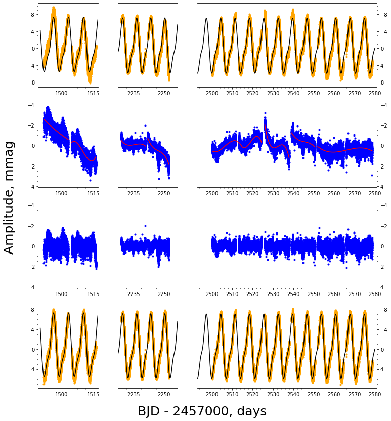
Figure 1: Outline of the detrending procedure of the TESS light curve (yellow) for the star HD 74521. The first panel from the top presents the original light curve where the green solid line describes harmonic model, the second panel shows the light curve pre-whitened with the inferred rotational frequency and its harmonic(s) where the red line the polynomial fit to the residuals, which is subtracted out to remove instrumental distortion, the third panel contains remaining noise with significantly reduced instrumental distortion, the fourth panel presents the final detrended light curve with green line harmonic model, removing the same polynomial fit as in the previous panel from the original light curve.

The Transiting Exoplanet Survey Satellite (TESS) space mission was launched on 2018 April 18 in order to detect exoplanets via high-precision photometry (Ricker et al., 2015). The data produced by this mission are extremely useful, as they allow the study of not only exoplanets, but variable stars as well. Here we are interested in CP stars that show rotational modulation and, in some cases (HD 24712), stellar pulsations (roAp type; Kurtz, 1978) in the presence of a magnetic field (Cunha et al., 2019; Holdsworth, 2021; Holdsworth et al., 2021). The observing plan for the primary TESS mission was to divide the celestial sphere into 26 sectors (with 24${}^{\circ}\times$96^∘ sky area covered by each sector), so that 13 sectors fall on each ecliptic hemisphere, and overlap near the ecliptic poles. The orbital period of the telescope around the Earth is 13.7 d (Gangestad et al., 2013), which corresponds exactly to half the length of the observation of each sector. One year of observation was dedicated to survey each hemisphere. The photometer works in two observing modes: full frame images (FFIs) from CCDs of each camera, whilst target pixel files (TPFs) collect data only from pixels encompassing pre-selected target stars. TESS accumulates data with a 30 min (FFIs) cadence for all stars, and with a 2 min (TPFs) cadence for approximately 200,000 objects that were accumulated from the accepted proposals for the primary mission observations (Stassun et al., 2018, 2019). After Cycle 2 the available modes have been expanded to 20 sec (TPFs) cadence and 10 min (FFIs) cadence observations.

We have used TESS data produced by the Science Processing Operations Center (SPOC) pipeline (Jenkins et al., 2016; Caldwell et al., 2020) and TESS light curves which are available from the Mikulski Archive for Space Telescopes (MAST) to carry out photometric analysis of selected ApBp stars that are expected to possess a significant magnetic field. We have selected a sample of eight relatively bright ApBp stars ($V<8.0$ mag) which show rotational modulation in their light curves with rotation periods longer than 2 d (see Table 1).

The selected ApBp stars possess relatively relatively low projected equatorial velocities ( $v\sin{i}<65$ km s^-1; see Table 1) that may indicate the presence of a hydrodynamically stable atmosphere. Fast rotation leads to mixing in the stellar atmosphere that affects or even destroys abundance stratification in the absence of a magnetic field (Michaud et al., 2015). Therefore, we selected for this study stars with rotation periods more than 2 d to ensure the hydrodynamic stability of their stellar atmosphere that is preferred for future analysis of abundance stratification. Knowledge of precise values of rotation periods will help carry out abundance analysis of these stars using Magnetic Doppler Imaging.

During the selection procedure we have used a database compiled by the TESS-AP procedure (Khalack et al., 2019, 2020) for stars observed by TESS with 2 min cadence. This procedure automatically performs a Fourier analysis of the light curves by employing the code period04 (Lenz & Breger, 2005) and collects stellar global parameters from the known astronomical databases (mainly from the TESS Input Catalogue (TIC; Stassun et al. 2018, 2019) and SIMBAD). The sample is not complete and includes only 8 interesting targets (see Table 1) selected to test our procedure for data reduction and analysis. Most of the selected targets have been observed in several sectors, which allowed us to effectively detrended their light curves and significantly reduce the instrumental distortions.

The instrumental distortions of a light curve are especially noticeable at the beginning and at the end of every 13.7 d segment of observations, corresponding to the TESS orbital period (see, for example, top panel of Fig. 1).

Since all the selected stars exhibit rotational modulation, the first step was to use the code period04 to detect and extract the rotational frequency and its dominant harmonics (no more than three frequencies in total) from the light curve using pre-whitening to obtain residuals with presumably only instrumental noise and distortions (see Fig. 1, second panel from the top). In general, the intervals for approximation were chosen as half the length of the observed sector or at the area between the gaps present in the light curve. It is worth emphasizing that at this stage one should choose carefully the intervals used for the polynomial fits, because an insufficient approximation leaves a significant amount of distortion. Meanwhile, an over-correction using a high-order polynomial (more than 3) introduces additional distortion to the light curve, which in turn may lead to a different value of the period of stellar rotation. Then, we approximated the instrumental distortions by a third-order polynomial with the aim to remove them and obtain residuals with random noise only (see Fig. 1, 3rd panel from the top). As the final step, the same polynomials were subtracted from the initial light curve to remove the instrumental distortions and obtain a light curve only with the rotational modulation, the remaining noise (see bottom panel at the Fig. 1), and also pulsation signals if present. A similar approach was used by Bowman et al. (2018) in the detrending of light curves of ApBp stars from the K2 mission.

We employed Monte Carlo simulations (Bevington, 1969) with the code period04 to determine the precision of defined frequencies which results in error bars of rotational periods. Error bars for the derived phases of the magnetic field measurements include the error of the period estimation. These error bars on the phase are small, given the tight constraints on the rotational periods and, in most cases, the relatively short intervals of time between the magnetic field measurements shown in the phase diagram plots and the time origin of the derived ephemerides.

2.2 Spectroscopy

For two stars (HD 22920 and HD 77314) we used unpolarized spectra obtained with the spectrograph HERMES (High-Efficiency and high-Resolution Mercator Echelle Spectrograph) at the Mercator telescope on La Palma.

The high-resolution fiber-fed prism-cross-dispersed echelle spectrograph HERMES covers the spectral domain from 3770 Å  to 9000 Å  in a single exposure with a resolution R = 85000 (Raskin et al., 2011), which is suited for abundance analysis. It is bench-mounted and kept in an environment with the pressure and temperature control to assure the stability of its work. With the HERMES spectrograph, we obtained spectra of HD 22920 and HD 77314 with a relatively high signal-to-noise ratio (SNR $\sim$ 300). The spectra were reduced using the dedicated data reduction pipeline HermesDRS (version 6.0) (Raskin et al., 2011), and used to derive effective temperature $T_{\rm eff}$, surface gravity $\log{g}$, radial velocity v_r and v$\sin{i}$ from analysis of Balmer line profiles (see Section 2.4 and Table 1).

2.3 Spectropolarimetry

The spectra have been obtained with the spectropolarimeter ESPaDOnS (Echelle SpectroPolarimetric Device for Observations of Stars) at the Canada-France-Hawaii Telescope (CFHT) and used to derive global stellar parameters (see Section 2.4) and to measure the mean longitudinal magnetic field $\langle B_{z}\rangle$ (see Section 2.5).

ESPaDOnS is capable of acquiring high resolution (R=65000) Stokes I and V spectra in the spectral domain from 3700 Å, to 10000 Å, with high SNR (in our case, spectra of targeted stars have SNR $>300$). The optical characteristics of this spectrograph, as well as its performances, were described by Donati et al. (2006) and Wade et al. (2016). The dedicated software package Libre-ESpRIT (Donati et al., 1997) was employed to reduce the obtained Stokes I spectra and the Stokes V circular polarisation spectra as well.

Two selected targets, HD 77314 and HD 86592, were monitored with dimaPol, a polarimeter module mounted at the entrance slit of the Cassegrain spectrograph installed on the 1.8-m Plaskett Telescope of the Dominion Astrophysical Observatory (DAO, Monin et al. 2015). It is used to carry out circular spectropolarimetry of magnetic stars with resolution R$\sim$10000 in a 280Å  wide spectral region centered on the $H_{\beta}$ Balmer line. By using Stokes V observations of the hydrogen $H_{\beta}$ line to measure the hemispherically averaged longitudinal magnetic field, dimaPol field measurements are less affected by rotational broadening than measurements based on metal lines, so that they are better suited to measure $\langle B_{z}\rangle$ in stars with relatively large values of v$\sin{i}$. For a description of the instrument and details of the typical data acquisition and reduction procedures see Monin et al. (2015).

2.4 Analysis of Balmer line profiles

We used the available high-resolution spectra of the selected targets to estimate their effective temperature and surface gravity, and to measure their radial velocities and v$\sin{i}$ values (see for detail Khalack & LeBlanc 2015). The Stokes I Balmer line profiles ($H_{\beta}$, $H_{\gamma}$, $H_{\delta}$, $H_{\epsilon}$, $H8$, $H9$, $H10$, $H11$, and sometimes $H12$) and the lines of metals located in the wings of Balmer lines were fitted by the theoretical profiles with the help of fitsb2 code (Napiwotzki et al., 2004) employing the grids of stellar atmosphere models (Husser et al., 2013) calculated using the phoenix-16 code (Hauschildt & Baron, 1999). The derived values of the global stellar parameters mostly fall into the range of estimation error bars compared to the previously published data (see Table 1) and to the results obtained in this study from the Geneva and Strömgren-Crawford photometry (see Table 2).

2.5 Measurements of the mean longitudinal magnetic field.

For each star, the measurements of the hemispherically averaged longitudinal magnetic field $\langle B_{\rm z}\rangle$ were extracted from the literature or derived from the analysis of available spectropolarimetric observations, and are presented in Table 3 and discussed in Section 3. The $\langle B_{\rm z}\rangle$ values have been derived from analysis of spectra obtained with different instruments (Donati et al., 2006; Bagnulo et al., 2015; Monin et al., 2015) and using different methods (Donati & Collier Cameron, 1997; Bagnulo et al., 2002; Kochukhov et al., 2010; Mathys, 2017), and may be inconsistent with each other. This information should be considered during analysis of $\langle B_{\rm z}\rangle$ variability with rotational phase.

We determined the mean longitudinal magnetic field $\langle B_{z}\rangle$ of HD 24712, HD 63401 and HD 74521 at the various epochs of observation by application of the moment technique to the Stokes I and V spectra of these stars that were observed with ESPaDOnS. The analysis procedure is as described by Mathys (2017). In short, in each spectrum, we measured the first order moments about the central wavelengths $\lambda_{0}$ of the Stokes V profiles of a set of selected diagnostic lines and performed a least-squares fit to derive the value of $\langle B_{z}\rangle$ from the slope of the linear dependence of these moments on the product of the effective Landé factors of the corresponding transitions by $\lambda_{0}^{2}$. We used the standard error of the longitudinal field that is derived from this least-squares analysis as an estimate of the uncertainty affecting the obtained value of $\langle B_{z}\rangle$. For HD 24712, we used Fe i lines as diagnostic lines, and for HD 74521, we employed Fe ii lines. Lines of these two ions were systematically used by Mathys (2017) for magnetic field determinations, on account of the fact that inhomogeneities in the distribution of iron over the surfaces of Ap stars tend to be moderate, so that measurements based on the analysis of Fe lines are mostly representative of the intensity and structure of the magnetic field itself. However, for HD 63401, whose $v\,\sin i$ is higher than for HD 24712 or HD 74521, the Fe lines proved ill-suited for magnetic field determination, so we used Si ii lines instead as diagnostic lines. Due to the highly non-uniform distribution of Si on the surface of HD 63401, these lines show considerable distortions, variable with rotation phase, which complicate their measurements. One should keep in mind that the derived $\langle B_{z}\rangle$ values are representative of the convolved contribution of the geometrical structure of the magnetic field and of the inhomogeneous distribution of Si.

Table 2: Stellar parameters derived from Strömgren-Crawford photometry ($T_{\rm eff}$ in column 2), from BC (log($L_{\star}$ in column 4), and from isochrone fitting for the studied stars (columns 3, 6, 8, 10). Data for stellar luminosity, radius and mass inferred from TIC 8 (Stassun et al., 2019) are shown for comparison in column 5, 7, 9 respectively. Data for the derived equatorial velocity are presented in the last two columns.

Name	$T_{\rm eff}$ (K)	$\log{g}$	log($L_{\star}$/ $L_{\sun}$)		$R$ ($R_{\sun}$)		$M_{\star}$ ($M_{\sun}$)		logAge	$v_{\rm eq}$ (km s-1)	$v_{\rm eq}/v_{\rm crit}$ ($\%$)
HD	This study	This study	This study	TIC	This study	TIC	This study	TIC	This study	This study	This study
	Photometry	Isochrone	BC cor.		Isochrone		Isochrone		Isochrone
10840	11489 $\pm$ 316	4.13(2)	1.97(3)	2.035(35)	2.452(3)	2.550(80)	2.923(1)	3.09(39)	8.224(3)	59.12(7)	12.40(2)
22920	13714 $\pm$ 386	3.91(2)	2.65(3)	2.424(320)	3.776(4)	-	4.152(1)	-	8.0734(4)	48.39(5)	10.57(2)
24712	7201 $\pm$ 290	4.16(6)	0.85(1)	0.863(15)	1.724(2)	1.715(70)	1.545(1)	1.63(27)	9.03(6)	7.00(1)	1.69(1)
38170	9493 $\pm$ 293	3.79(2)	1.94(3)	2.006(34)	3.463(3)	3.354(142)	2.6762(7)	2.56(35)	8.6324(3)	63.32(5)	16.50(2)
63401	13201 $\pm$ 380	4.15(2)	2.27(3)	-	2.617(3)	-	3.526(1)	-	7.946(2)	54.82(2)	10.82(2)
74521	10474 $\pm$ 285	3.80(2)	2.16(3)	-	3.657(3)	-	3.034(1)	-	8.4811(3)	26.24(2)	6.60(1)
86592	7716 $\pm$ 336	4.08(6)	1.10(1)	1.150(23)	2.003(3)	1.895(60)	1.7482(5)	1.981(300)	8.986(2)	35.10(5)	8.61(2)

For HD 77314 and HD 86592, the reported $\langle B_{z}\rangle$ measurements (see Table 3) have been obtained with dimaPol (Monin et al., 2015), which are less affected by considerable rotational broadening of this targets due to the designed qualities of this unique instrument (see Section 2.3).

The timestamps of flux and $\langle B_{\rm z}\rangle$ measurements were converted to the Barycentric Julian Date to use the same time units to plot the light curve and magnetic field phase diagrams. Since the rotation periods obtained from photometric observations were used to build a phase diagram for most stars, the zero phase for the magnetic and photometric data was set at the minimum closest to the beginning of the analysed light curve.

2.6 Geneva and Strömgren-Crawford photometry

Geneva and Strömgren-Crawford photometric indices were used to determine the effective temperature as the first step in evaluation of the luminosity by using the method of bolometric correction (BC) (Flower, 1996), and radius through stellar isochrone fitting (Sichevskij, 2017). The derived stellar parameters (see Table 2) were employed to determine the rotational rate $v_{\rm eq}/v_{\rm crit}$ for the stars described in this study.

For the Geneva photometry, the General Catalogue of Photometric Data by Paunzen (2015) was used. The values of $c1$, $m1$, and $(b-y)$ for the uvby$\beta$ photometry were taken from the Hauck & Mermilliod (1998) catalogue. Unfortunately, one star (HD77314) was left out of consideration because there are no data available for this object. To determine the value of $[u-b]$, we used the original formulae described by Strömgren (1966) as $[u-b]=[c1]+2[m1]$, where reddening free indices are calculated from $[m1]=m1+0.18(b-y)$ and $[c1]=c1-0.20(b-y)$. Then, we have used the formulae for variable $\theta_{\rm eff}$ specified for CP2 stars to calibrate the effective temperature

$$\theta_{\rm eff}=0.234(0.009)+0.213(0.008)[u-b]~{},$$ (1)

Netopil et al. (2008) (for the uvby$\beta$ photometry) and

$$\theta_{\rm eff}=0.835(0.028)+0.458(0.013)(B2-G)^{0}~{},$$ (2)

(Hauck & North, 1982) (for the Geneva photometry). Rufener (1988) reported that the standard deviation of colors in the Geneva photometry is around 0.001 mag. The final values of effective temperature are obtained from $\theta_{\rm eff}=5040/T_{\rm eff}$ (Napiwotzki et al., 1993).

The value of BC is calculated taking into account the coefficients from Flower (1996) and the effective temperature obtained from photometry. To derive stellar luminosity $\log(L/L_{\sun})$:

$$\log(L/L_{\sun})=-0.4[M_{V}-V_{\sun}-31.572+(BC_{V}-BC_{V,\sun})]$$ (3)

we have employed the $BC_{V,\sun}$ = $-0.08$ and the apparent magnitude of the Sun $V_{\sun}$ = $-26.75\pm 0.03$ which are introduced by Cox (2000) and later adjusted by Torres (2010). To determine the absolute magnitude $M_{V}$, we have used values of the derived parallax from Gaia EDR3 and apparent magnitude in V band from the Hipparcos catalogue.

The Stellar Isochrone Fitting Tool was used to estimate stellar age, radius and mass with the methods described by Sichevskij (2017). Parameters were determined from evolutionary track models of solar metallicity $Z=0.014$ (Bressan et al., 2012), according to the given temperature and luminosity. Using the following relation for the equatorial velocity (Netopil et al., 2017), where the stellar radius is expressed in the units of solar radius $R_{\sun}$,

$$v_{\rm eq}({\rm kms^{-1}})=50.579R(R_{\sun})/P_{\rm rot}({\rm d})$$ (4)

we are able to derive the critical rotational fraction $v_{\rm eq}/v_{\rm crit}$. Considering the formula provided for critical velocity $v_{\rm crit}$ by Georgy et al. (2013), we have derived the following expression for the rotation rate:

$$v_{\rm eq}/v_{\rm crit}=\frac{50.579R_{\rm eq}(R_{\sun})}{P_{\rm rot}}\sqrt{\frac{R_{\rm eq}(R_{\sun})}{GM_{\star}(M_{\sun})}}$$ (5)

where equatorial radius $R_{\rm eq}(R_{\sun})$, stellar mass $M_{\star}(M_{\sun})$ are expressed in respective solar units, and $G$ stands for the universal gravitational constant.

Summarising the procedure described above we have collected the data in Table 2 and compared them to the values extracted from the TIC 8 catalogue (Stassun et al., 2018, 2019). The age derived for each target is measured in years (see column 10 of Table 2). The combination of the stellar parameters derived from the analysis of Balmer line profiles, from Geneva and Strömgren-Crawford photometry (see Table 2), and from the literature (see Table 1) in most cases points to the same values considering estimation error bars. Three stars, HD 74521, HD 86592, and HD 10840 are exceptions. HD 74521 shows a large discrepancy between $\log{g}$ determined from isochrone fitting and the TIC, and for $T_{\rm eff}$ in values extracted from the TIC while values derived from Balmer lines and Strömgren-Crawford photometry matched. Discrepancy occurred also to the values $R$ and log($L_{\star}$/ $L_{\sun}$) considering their error-bars obtained for stars HD 10840 and HD 86592 from the TIC and from the isochrone fitting.

3 Results of analysis of individual stars

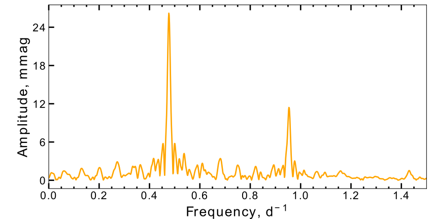
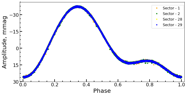
Figure 2: Periodogram (top panel) and phase diagram (bottom panel) built for the rotational period $\emph{P}=2.0976858$ d in HD 10840 using the reduced 2 min cadence light curve from the sectors 1 - 2 and 10 min cadence light curve from the sectors 28-29.

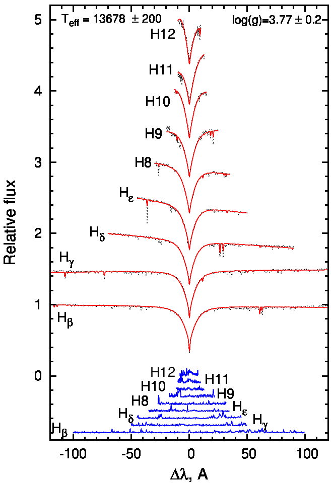
Figure 3: The synthetic spectra (thin dotted lines) are fitting well the Balmer line profiles (thick lines) observed by NARVAL for HD 22920 assuming $T_{\rm eff}=13700\pm 200$ K and $\log{g}=3.8\pm 0.2$ and metallicity $M=-0.5$. For the purpose of visual convenience, Balmer lines are shifted by 0.5. Difference between the synthetic and observed spectra is shown by blue lines below.

3.1 HD 10840 (TIC 231844926 = BM Hyi)

According to the catalog of Houk & Cowley (1975) HD 10840 is classified as a CP star of ApSi type and is on the boundary between the spectral types A and B taking into account its effective temperature $T_{\rm eff}=11600$ K and surface gravity $\log{g}=3.60$ (Bailey & Landstreet, 2013). Renson & Manfroid (1992) provided for this star a spectral type of B9. Levato et al. (1996) derived radial velocity v${}_{\rm r}=19.4\pm 2.1$ km s^-1 and v$\sin{i}<30$ km s^-1. Bailey & Landstreet (2013) determined its v$\sin{i}$ = 35$\pm$5 km s^-1.

Measurement of the mean longitudinal magnetic field of HD 10840 were obtained by Kochukhov & Bagnulo (2006) and Bagnulo et al. (2015). Kochukhov & Bagnulo (2006) used the method developed by Bagnulo et al. (2002) to derive the mean longitudinal magnetic field from analysis of circular polarisation detected in FORS1 spectra in the area of the Balmer line profiles. Bagnulo et al. (2015) employed the same method to analyze the same FORS1 spectrum of HD 10840, but taking into account the polarisation detected in the Balmer and metal line profiles (see Table 3). Bailey & Landstreet (2013) used a simple magnetic dipole model with the adopted field strength at the magnetic pole, $B_{\rm d}$=500 G, to fit the magnetically sensitive line profiles of Ti, Cr, Fe and Si found in the available spectra of HD 10840.

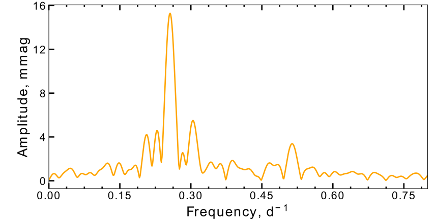
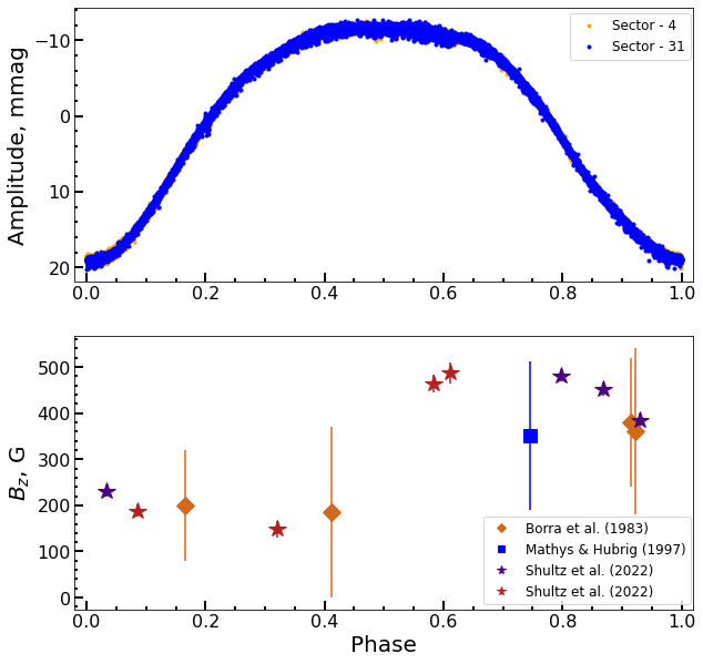
Figure 4: Periodogram (top panel) and phase diagram (middle panel) built for rotational period 3.947225 d of HD 22920 using the reduced light curve obtained from sectors 4 and 31. The bottom panel shows phase diagram built on the measurements of the mean longitudinal magnetic field taken from Borra et al. (1983) (brown diamonds), Mathys & Hubrig (1997) (blue squares). We show also the LSD measurements of the mean longitudinal magnetic field obtained by Shultz et al. (2022) from NARVAL (red stars) and ESPaDOnS (indigo stars) spectra.

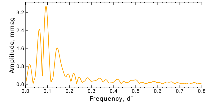
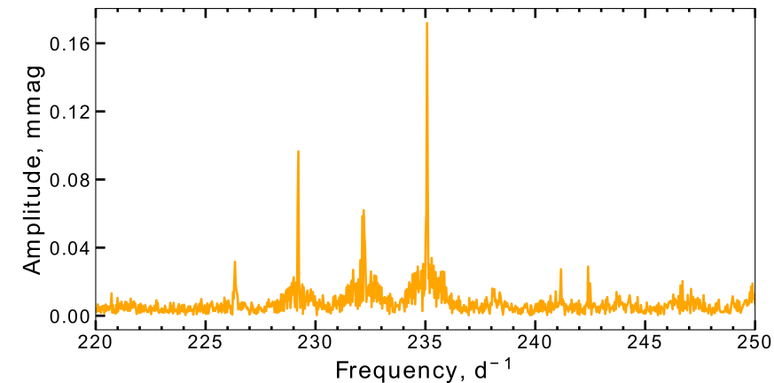
Figure 5: Discrete Fourier transform of the reduced light curve obtained by TESS for HD 24712 in the sector 5 and 31. Significant signals are detected at low frequencies (top panel) that correspond to stellar rotation, and at the high frequencies (bottom panel) that correspond to roAp pulsations.

The period $\emph{P}=2.097679(7)$ d of stellar rotation of HD 10840 was determined by Sikora et al. (2019c) from the analysis of photometric data obtained with the space telescope TESS in sectors 1-2. In our study, we measure a more precise value of the rotation period as $\emph{P}=2.0976858(2)$ d which is compatible with that from Sikora et al. (2019c). It was derived from the analysis of detrended light curves obtained for this star in sectors 1 and 2 with 2 min cadence and in sectors 28 and 29 with 10 min cadence.

The upper panel of Fig. 2 presents the low-frequency region of the discrete Fourier transform of the reduced light curve of HD 10840. From the Fourier analysis we identified a signal at $\nu=0.47671583(5)$ d^-1 and its first harmonic. In this case, the derived lower frequency, which appears to be the tallest peak, is identified as the frequency of stellar rotation.The lower panel of Fig. 2 shows the phase diagram built using the derived rotational period.

3.2 HD 22920 (TIC 301621458 = FY Eri)

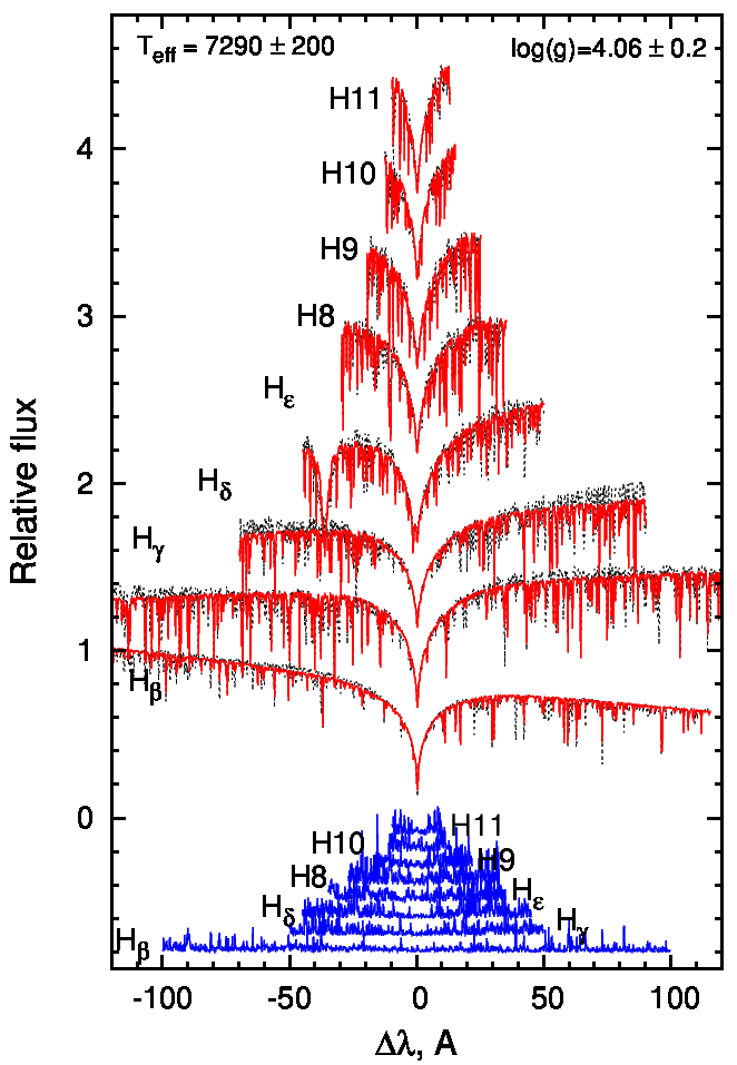
Figure 6: The same as in Fig. 3 but the best fit of Balmer line profiles in HD 24712 is obtained for $T_{\rm eff}=7300\pm 200$ K and $\log{g}=4.1\pm 0.2$.

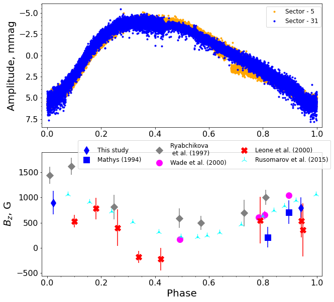
Figure 7: Phase diagram of HD 24712 is built using the derived rotational period $\emph{P}=12.24267$ d for the reduced light curve from the sector 5 and 31, and for the $\langle B_{\rm z}\rangle$ measurement from Wade et al. (2000) (pink circles), Mathys (1994) (blue squares), and Leone et al. (2000) (red cross).

HD 22920 was reported by Cowley et al. (1968) as a variable CP star of spectral type B8pSi, and the most recently determined spectral type is B8II (Houk & Swift, 1999). Leone & Manfre (1996) found for this star $T_{\rm eff}=13800$ K and $\log{g}=3.65$, which are close to the estimates of $T_{\rm eff}=13700$ K and $\log{g}=3.72$ obtained by Catanzaro et al. (1999) and to the results $T_{\rm eff}=13640$ K and $\log{g}=3.74$ derived by Khalack & LeBlanc (2015). From the recently obtained ESPaDOnS spectropolarimetric data, we measured the values of $T_{\rm eff}=13700\pm 200$ K and $\log{g}=3.8\pm 0.2$ from fitting Balmer line profiles with the help of the fitsb2 code (Napiwotzki et al., 2004) (see Fig. 3).

From the analysis of nine Balmer line profiles, Khalack & Poitras (2015) estimated $T_{\rm eff}$= 13640 K and $\log{g}$ = 3.72. The LTE model of the stellar atmosphere has been calculated by Khalack & Poitras (2015) employing the code PHOENIX (Hauschildt et al., 1997) for the derived effective temperature and $\log{g}$ to carry out the line profile simulations with the help of the zeeman code (Landstreet, 1982). This analysis demonstrated that HD 22920 has inhomogeneous abundance distribution of chemical elements in its atmosphere considering that it shows a variability of line profiles for the studied ions.

Mathys & Hubrig (1997) and Borra et al. (1983) analysed spectropolarimetric data obtained by using the Zeeman analyzer at Cassegrain Echelle Spectrograph (CASPEC) and photoelectric Pockels cell polarimeter respectively, and derived the mean longitudinal magnetic field in the different rotational phases of HD 22920 (see Table 3). Glagolevskij (2007) calculated the root-mean-square magnetic field (line-of-sight component) $<B_{\rm e}>=148\pm 50$ G and average surface magnetic field $B_{\rm s}=800$ G. Applying the least-squares deconvolution (LSD) method (Donati & Collier Cameron, 1997; Kochukhov et al., 2010) to the available ESPaDOnS and NARVAL spectra of HD 22920, Shultz et al. (2022) measured the mean longitudinal magnetic field (see Table 3) for an additional eight rotational phases and provided a precise value for the dipolar magnetic field $B_{\rm d}=1.6^{+1.1}_{-0.0}$ kG.

Bartholdi (1988) found that this star shows a periodic variability in Geneva 7-color photometry with $\emph{P}=3.95$ d. The value of this period was recently refined to $\emph{P}=3.9489(3)$ d from the MASCARA photometric survey (Bernhard et al., 2020), and to the period $\emph{P}=3.9472(1)$ d found by Shultz et al. (2022) via the fitting of $<B_{\rm z}>$ measurements. Based on our detrended light curve from sectors 4 and 31 we have determined the value of the rotation period to be $\emph{P}=3.947225(2)$ d for HD 22920 which is in good accordance with the result published by Shultz et al. (2022). The top panel of Fig. 4 shows the discrete Fourier transform of the reduced light curve at low frequencies for HD 22920. We have used the derived period to build a phase diagram of the light curve (see middle panel of Fig. 4) and magnetic field measurements (see bottom panel of Fig. 4). One can see from the bottom panel of Fig. 4 that the mean longitudinal magnetic field reaches its minimum at the phase $\varphi\simeq$ 0.3 when the light curve is close to its maximum, and increases to maximum field at the phase $\varphi\simeq$ 0.7 while the light curve is decreasing. It appears that the magnetic field influences the departure from horizontal uniformity of the chemical composition in stellar atmosphere of HD 22920, which in turn causes the observed rotational modulation of the light curve assuming the oblique rotator model.

3.3 HD 24712 (TIC 279485093 = DO Eri)

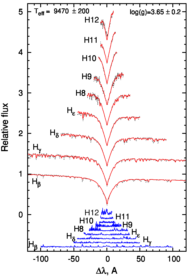
Figure 8: The same type of analysis as in Fig. 3 but the best fit of Balmer lines in HD 38170 is obtained for $T_{\rm eff}=9500\pm 200$ K and $\log{g}=3.65\pm 0.2$.

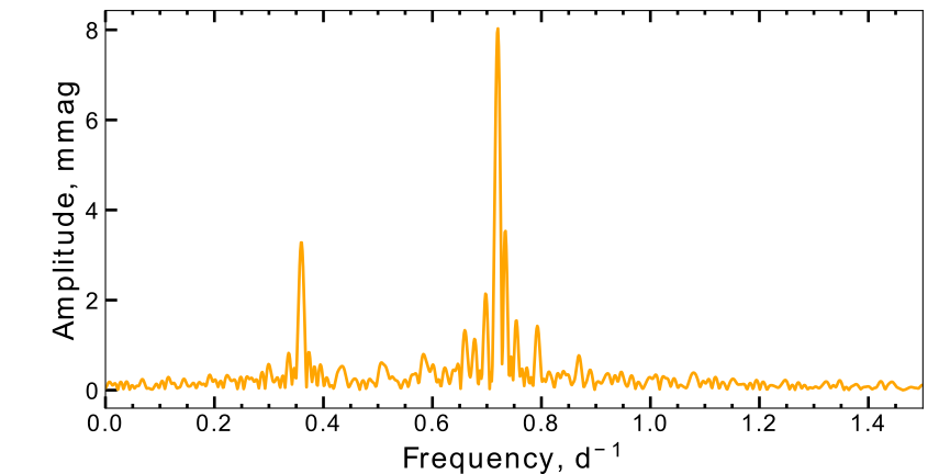
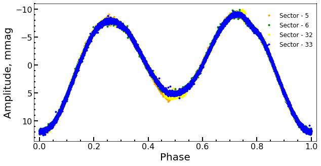
Figure 9: The same as at the Fig 2 but for HD 38170. The phase diagram is built using the rotational period $\emph{P}=2.766116$ d derived from the reduced light curve observed in the sector 5, 6, 32 and 33.

HD 24712 is one of the best-studied rapidly oscillating (roAp) chemically peculiar stars. Abt & Morrell (1995) determined that HD 24712 is a variable star of spectral type A9Vp SrEuCr. Preston (1972) measured for this star the values of v$\sin{i}=7.0$ km s^-1 and $i=40^{\circ}$. In the study of mCP stars Sikora et al. (2019a) derived measurements of v$\sin{i}=6.6\pm 0.6$ km s^-1 and $\log{g}=3.8\pm 1.0$ from spectroscopy. Ryabchikova et al. (1997) provide the values of $T_{\rm eff}=7250$ K and $\log{g}=4.2$ from the photometric and spectroscopic observations as well as magnetic measurements. Using available spectroscopic data we determine $T_{\rm eff}=7300\pm 200$ K, $\log{g}=4.1\pm 0.2$ from the analysis of Balmer line profiles (see Fig. 6) which are in a good accordance with the previously published data considering the estimated error bars.

Assuming the oblique rotator model, Preston (1972) derived a rotation period of $\emph{P}=12.448$ d from the EWs of metal lines. Later, Kurtz & Marang (1987) improved the estimation of the photometric rotational period to 12.4572(3) d. Using Fourier analysis for measurements of circular and linear polarisation, Bagnulo et al. (1995) derived the period of stellar rotation $\emph{P}=12.461(1)$ d which is in good accordance with the value obtained by Mathys (1991).

The extensive spectroscopic and polarimetric study of HD 24712 by Ryabchikova et al. (2007) determined the phase shifts for the different elements according to the pulsation peak between radial velocity and photometric data which allow estimation of the propagation of pulsation maximum. The available measurements of the mean longitudinal magnetic field starting from Preston (1972) up till now are presented in Table 3. Measurements of the mean longitudinal magnetic field were obtained with the CASPEC Zeeman analyzer by Mathys (1994) which measured the wavelength shifts between right and left circular polarizations. Leone et al. (2000) estimated the mean longitudinal magnetic field by using the same method applied to the polarimetric spectra obtained with the fiber-fed REOSC spectrograph of the Catania Astronomical Observatory. Wade et al. (2000) provided the mean longitudinal magnetic field derived with high-precision from LSD Stokes V profiles by using the MuSiCoS spectropolarimeter. Rusomarov et al. (2013) reported with high accuracy 15 new measurements of $<B_{\rm z}>$ (see Table 3) derived from analysis of LSD Stokes V profiles obtained for iron and rare earth elements by using HARPSpol’s polarimetric spectra. From available measurements, these authors determined the parameters for a model of inclined magnetic dipole and determined the rotational period $\emph{P}=12.45812(19)$ d. Rusomarov et al. (2015) used magnetic Doppler imaging to provide a detailed magnetic field topology where dipolar components play a key role with a small impact from high-order harmonics.

Unlike the other stars in our sample, the detrending procedure for HD 24712 was applied separately to each sector. Since the star demonstrates not only rotational modulation but also pulsations inherent to the roAp subclass, we performed prewhitening of high-order frequencies of stellar pulsation as well. From Fourier analysis of TESS photometric data combined from Sectors 5 and 31, we detected a signal at the frequency (and its first harmonic) that correspond to the period of rotation $\emph{P}=12.45862(5)$ d. The period determined in this article appears to be larger by 2 $\sigma$ than to the value obtained by Rusomarov et al. (2015). The top panel in Fig. 5 shows a significant signal detected at the low frequencies of the discrete Fourier transform of the reduced light curve. High-frequency roAp oscillations were discovered in HD 24712 by Kurtz (1981), with the p-mode pulsation period being 6.15 min. We have detected p-mode pulsations at high frequencies (see bottom panel in Fig. 5) and we determined the pulsation period $\emph{P}=6.1257(1)$ min corresponding to the strongest signal. From the analysis of three frequencies having the most significant amplitudes at the following frequencies 235.07495 d^-1, 232.19730 d^-1, 229.20934 d^-1, we estimated the average separation to be about 2.93281 d^-1.

3.4 HD 38170 (TIC 140288359 = WZ Col)

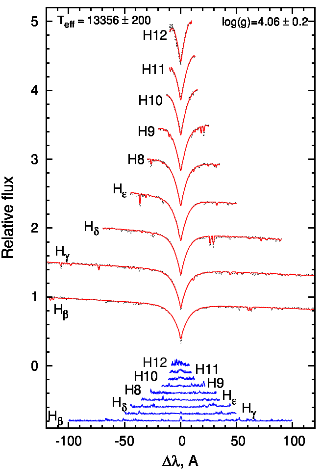
Figure 10: The same type of analysis as in Fig. 3 except for the synthetic lines of the star HD 63401 were used the value of $T_{\rm eff}=13400\pm 200$ K and $\log{g}=4.1\pm 0.2$.

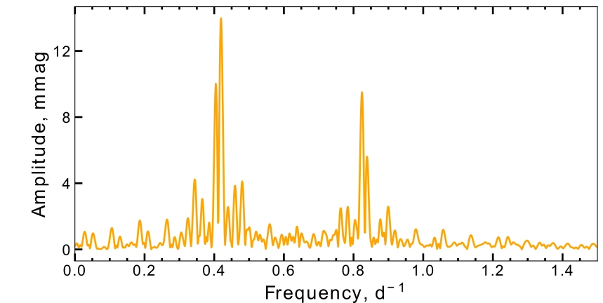
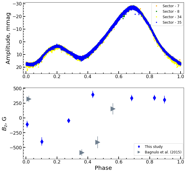
Figure 11: The same as at the Fig 4 but for HD 63401. Phase diagram is built using the derived rotational period $\emph{P}=2.414474$ for the reduced light curve from the sectors 7,8, and 34,35 and for $<B_{\rm z}>$ measurements from Bagnulo et al. (2015) (black triangles).

HD 38170 has been identified as a CP star with the spectral class B9 by Cannon & Pickering (1993). The radial velocity has been obtained in many studies and the values are clustered around 35 km s^-1, but the most recent measurement $36.3\pm 0.6$ km s^-1 has been provided by Gontcharov (2006). From the Fourier transform analysis of line profiles, Royer et al. (2002) derived v$\sin{i}$ = $65\pm 9$ km s^-1. Zorec & Royer (2012) derived a stellar mass of $M=3.07\pm 0.05(M_{\sun})$, fractional age on the main sequence $0.89\pm 0.04$, and other fundamental parameters, such as $T_{\rm eff}$ = $10000\pm 257$ K and log$(L_{\star}/L_{\sun})=2.17\pm 0.03$, from Strömgren-Crawford photometry. Similar mass $M=2.8\pm 0.1(M_{\sun})$ and age $394^{+10}_{-17}$ Myr, which corresponds to log(Age) = $8.60^{+0.02}_{-0.04}$ yr, were obtained by David-Uraz et al. (2021) for HD 38170. From the analysis of Balmer line profiles we determined $T_{\rm eff}=9500\pm 200$ K and $\log{g}=3.65\pm 0.2$ (see Fig. 8).

David-Uraz et al. (2021) confirmed that HD 38170 is a magnetic CP star via direct detection in Stokes V profiles obtained with ESPaDOnS (see Table 3) and calculated its dipolar magnetic strength as $B_{\rm d}=254^{+78}_{-49}$ G by applying a Bayesian analysis on LSD profiles (Petit & Wade, 2012). From the TESS first year observations David-Uraz et al. (2021) determined the rotation period $\emph{P}=2.76618(4)$ d and measured v$\sin{i}=57\pm 5$ km s^-1. The global stellar parameters obtained in this study for HD 38170 are quite similar to those presented by David-Uraz et al. (2021) considering estimation error bars, except for the mass that is different by more than 1 $\sigma$ (see Table 2).

From the TESS observations we were able to identify the rotational period for HD 38170. From Fourier transform analysis (see Fig. 9) we defined a signal at the low-frequency region that may be interpreted as the first harmonic. We have detrended the light curve of this star obtained by TESS in sectors 5, 6, 32 and 33, and phased it with the period of stellar rotation (see the lower panel of Fig. 9). On the phase diagram, one can clearly see two maxima that most probably appear due to the presence of abundance spots in the stellar atmosphere of HD 38170. Contrary to the case of HD 10840 (see Subsection 3.1), the highest peak for HD 38170 is found at larger frequency (second one).The rotational period 2.766116(2) d determined for this frequency is consistent with the result derived by David-Uraz et al. (2021).

3.5 HD 63401 (TIC 175604551 = OX Pup)

Figure 12: The same as in Fig. 3 but for best fit of Balmer lines in HD 74521 obtained for $T_{\rm eff}=10600\pm 200$ K and $\log{g}=3.5\pm 0.2$.

Figure 13: The same as at the Fig 4 but for HD 74521. Phase diagram is built using the derived rotational period $\emph{P}=7.05010$ d for the reduced light curve from the sectors 7, 34 and 44 to 46 and for the $\langle B_{\rm z}\rangle$ measurements from Bohlender et al. (1993) (green pentagons), Mathys (1994) (blue squares and diamonds (private)) and Leone (2007) (red stars).

The star HD 63401 was classified as a variable star of spectral type B9 (Cannon & Pickering, 1993). Bailey et al. (2014) provided for HD 63401, $T_{\rm eff}=13500\pm 500$ K which was previously mentioned by Landstreet et al. (2007), and derived $\log{g}=4.2\pm 0.2$ and v$\sin{i}=52\pm 4$ km s^-1 from the analysis of two FEROS spectra. The radial velocity v${}_{\rm r}=22.0\pm 1.4$ km s^-1 (see Table 1) was derived for HD 63401 by Gontcharov (2006). We report for HD 63401 similar stellar parameters $T_{\rm eff}=13400\pm 200$ K, $\log{g}=4.1\pm 0.2$, v${}_{\rm r}=26\pm 2$ km s^-1 and v$\sin{i}=52\pm 4$ km s^-1 obtained from the fitting of Balmer line profiles in the available ESPaDOnS spectra (see Fig. 10).

Glagolevskij (2007) studied HD 63401 and determined the mean longitudinal magnetic field (line-of-sight component) $<B_{\rm e}>=70\pm 50$ G and the root-mean-square magnetic field $B_{\rm rms}=400$ G. Landstreet et al. (2007) derived the value $B_{\rm rms}=365$ G, which is in good accordance with the result obtained by Glagolevskij (2007). Bagnulo et al. (2015) used polarimetric spectra obtained with the spectrograph FORS1, and measured the mean longitudinal magnetic field from the analysis of circular polarisation in the Balmer line profiles and metal lines (see first column in Table 3).

The period of stellar rotation $2.41\pm 0.02$ d was derived from the analysis of the light curves observed at ESO, with the ESO 50 cm telescope and the Danish 50 cm telescope, and reported for the first time by Hensberge et al. (1976). From the available photometric TESS data, we confirm the value of the above period. The top panel of the Fig. 11 presents the discrete Fourier transform of the reduced light curve observed by TESS in sectors 7, 8, 34 and 35. The significant signals detected at low frequency and its first harmonic may be caused by stellar rotation with the period $\emph{P}=2.414474(1)$ d. In the middle panel in Fig. 11, we show the phased light curve with period of rotation determined from reduced TESS data. Looking for a precise period of rotation, we applied Fourier transform to combined $<B_{\rm z}>$ measurements from published data (Bagnulo et al., 2015) and this study in the vicinity of the fundamental rotational frequency determined from the TESS data. This attempt to obtain a more precise period was motivated by the observed phase shift between two $<B_{\rm z}>$ datasets when folded with the period derived from TESS data (see bottom panel in Fig. 11). In result, the proper phasing of magnetic field measurements using the photometric period was unsuccessful.

3.6 HD 74521 (TIC 443995718 = BI Cnc)

Figure 14: The same type of analysis as in Fig. 3 except for the synthetic lines of the star HD 77314 were used the value of $T_{\rm eff}=11400\pm 200$ K and $\log{g}=4.0\pm 0.2$.

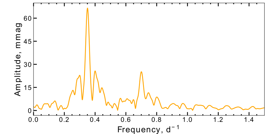
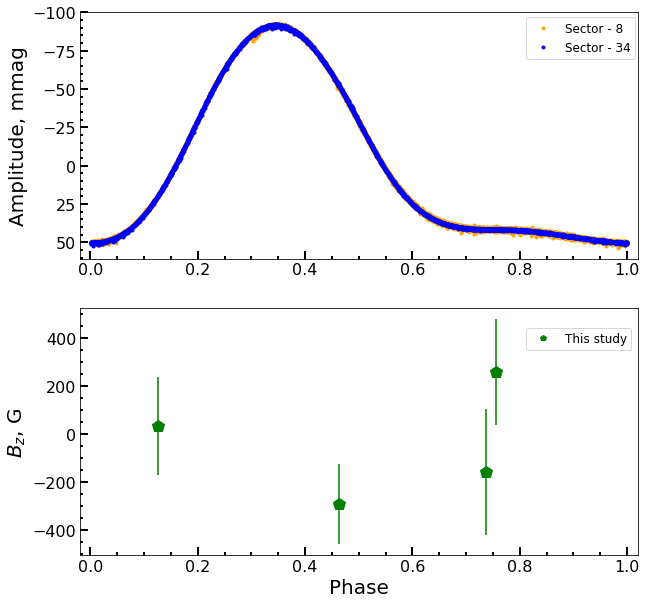
Figure 15: The same as at the Fig 4 but for HD 77314. The phase diagram is built using the derived rotational period $\emph{P}=2.864325$ for the reduced light curve from the sectors 8 and 34 and for $<B_{\rm z}>$ DAO longitudinal magnetic field measurements (green pentagons).

Abt & Morrell (1995) provided the spectral type A1Vp for HD 74521 with HgMnSiEu strong lines and CaMg weak lines, and v$\sin{i}=10$ km s^-1. Royer et al. (2002) used Fourier transform analysis of line profiles in the range 420-460 nm to combine the set of rotational velocities for Ap stars on the basis of the previous study of Abt & Morrell (1995), and derived for HD 74521 v$\sin{i}=18.0\pm 0.9$ km s^-1, and Mathys (1995) determined v$\sin{i}=19.0\pm 4.6$ km s^-1. Gontcharov (2006) provided the value of radial velocity v${}_{\rm r}=27.5\pm 1.4$ km s^-1. Wraight et al. (2012) provided for HD 74521 an effective temperature of $T_{\rm eff}=10789\pm 500$ K. Our estimates of $T_{\rm eff}=10600\pm 200$ K derived from the fitting of Balmer lines (see Fig. 12) and $T_{\rm eff}=10500\pm 300$ K inferred from the Strömgren-Crawford photometry (see Table 2) are consistent with the results of Wraight et al. (2012) considering the estimated uncertainties. Also, from the analysis of Balmer line profiles we have obtained v$\sin{i}=18\pm 3$ km s^-1 and v${}_{\rm r}=24\pm 3$ km s^-1 which are in good accordance with the previously published data taking into account the estimation error bars (see Table 1).

HD 74521 was investigated as a mCP star since Stepien (1968) who measured the period of stellar rotation to be $\emph{P}=5.43$ d. During the last decades, many rotation periods were derived for HD 74521 from terrestrial and space observations. Recent measurements have been obtained by Leone (2007) as $\emph{P}=7.0486(5)$ d, $\emph{P}=6.91(1)$ d by Wraight et al. (2012) and $\emph{P}=7.0501(2)$ d by Dukes & Adelman (2018).

TESS has carried out observations of HD 74521 in sectors 7, 34 and 44 to 46, which provide a valuable time baseline of almost 3 yr. From the discrete Fourier transform of the reduced light curve, we confirm the value of the rotational period to be $\emph{P}=7.05010(5)$ d. The top panel of Fig. 13 shows a significant signal at $\nu=0.1418419(1)$ d^-1 that is related to stellar rotation. The middle and bottom panels of Fig. 13 present a phase diagram. The measurements of the mean longitudinal magnetic field are taken from Bohlender et al. (1993), Mathys (1994) and Leone (2007). The mean longitudinal magnetic field was measured with the Pockels cell polarimeter and the CASPEC Zeeman analyzer respectively. Leone (2007) measured the mean longitudinal magnetic field across the whole spectrum and through Balmer lines obtained with the spectropolarimeter ISIS. New three $<B_{\rm z}>$ measurements were derived for this object using high-resolution spectropolarimetric data recently obtained with ESPaDOnS. Even though the mean longitudinal magnetic field is consistently detected at the level of several hundred G, different $<B_{\rm z}>$ datasets show systematic differences with very low or approaching zero variability in each.

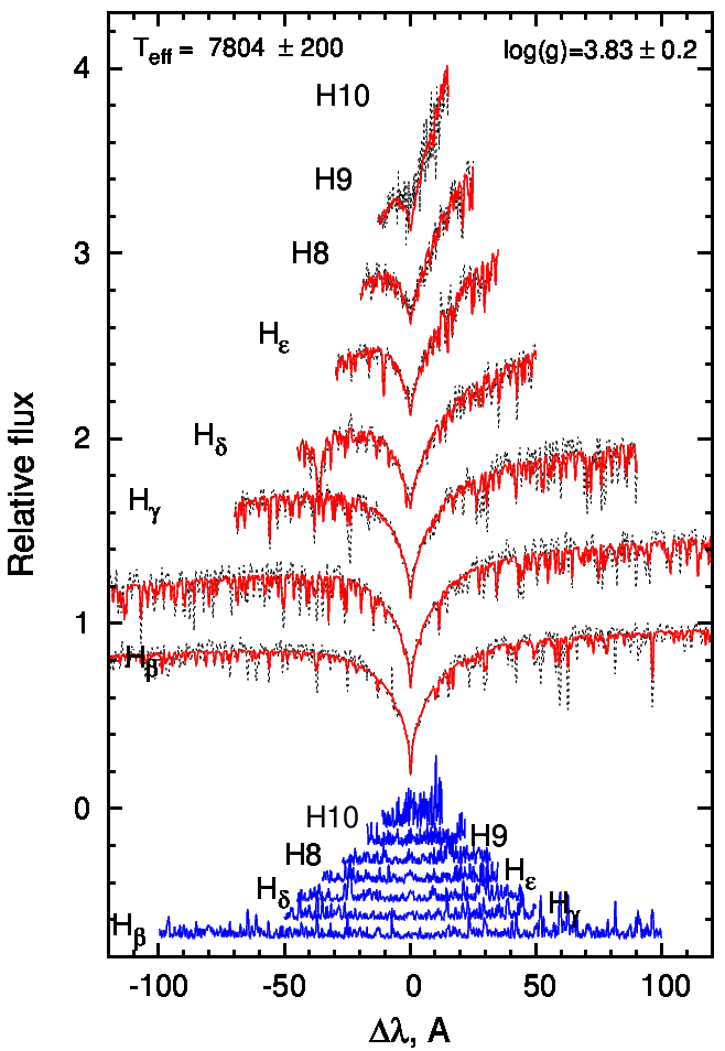
Figure 16: The same as in Fig. 3 but for best fit of Balmer lines in HD 86592 obtained for $T_{\rm eff}=7800\pm 200$ K and $\log{g}=3.8\pm 0.2$.

3.7 HD 77314 (TIC 270487298 = NP Hya)

HD 77314 is a CP star of spectral type A2 (Cannon & Pickering, 1993), or alternative type ApSrCrEu (Houk & Swift, 1999). The TESS input catalogue (TIC) provides the effective temperature $T_{\rm eff}=9253\pm 372$ K and surface gravity $\log{g}=3.69\pm 0.10$ (Stassun et al., 2018, 2019). From the fitting of Balmer line profiles in the HERMES spectra (see Fig 14) we have derived $T_{\rm eff}=11400\pm 200$ K and $\log{g}=4.0\pm 0.2$ (see Tables 1, 2). As there was no data available in the Geneva and Strömgren-Crawford photometry catalogs, we could not confirm any of the above data, which are in stark disagreement.

From the extensive study of rotational periods from MASCARA data, Bernhard et al. (2020) derived the rotation period of $\emph{P}=2.86445(8)$ d which is in a good accordance with the period of $\emph{P}=2.8646$ d presented in the International Variable Star Index of the American Association of Variable Star Observers (VSX; Watson et al., 2006). From the discrete Fourier transform of the detrended light curve observed in sectors 8 (2 min cadence) and 34 (10 min cadence) (see top panel Fig 15) we have detected the signals in the low-frequency region that most probably correspond to the rotation period $\emph{P}=2.864325(1)$ d which deviates from the period determined by Bernhard et al. (2020) by more than 1 $\sigma$. In the bottom panels of Fig 15, we provide the phase diagram built with this period for the light curve and for the measurements of the mean longitudinal magnetic field. Considering the obtained error bars the derived $\langle B_{\rm z}\rangle$ measurements do not appear to differ significantly from zero. We need to use Stokes I and V spectra with higher signal to noise ratio for HD 77314 (e.g. from ESPaDOnS) to measure its magnetic field with high precision.

3.8 HD 86592 (TIC 332654682 = V359 Hya)

Houk & Smith-Moore (1988) determined the spectral type of HD 86592 as ApSrEuCr. In this study, the effective temperature $T_{\rm eff}=7800\pm 200$ K and surface gravity $\log{g}=3.8\pm 0.2$ are estimated for HD 86592 from the fitting of Balmer line profiles observed with HERMES (see Fig. 16). Considering the estimated uncertainties these data are consistent with the values of $T_{\rm eff}=7955\pm 95$ K and $\log{g}=4.28\pm 0.18$ from Kordopatis et al. (2013) and to our estimates of $T_{\rm eff}=7700\pm 300$ K and $\log{g}=4.08\pm 0.06$ obtained for this star from the Geneva photometry (see Table 2).

The presence of a strong magnetic field did not allow Babel & North (1997) to estimate the value of rotational velocity from individual line profiles, therefore, they used the correlation dip and derived the values v${}_{\rm r}=12.7\pm 0.3$ km s^-1 and v$\sin{i}=16\pm 2$ km s^-1 for HD 86592. Our estimate of the radial velocity v${}_{\rm r}=13\pm 1$ km s^-1 is in a good accordance with the published value, while v$\sin{i}=27\pm 5$ km s^-1 appears to be overestimated due to the magnetic widening of line profiles and other line broadening factors. The study of magnetic fields of cool CP stars leads Babel & North (1997) to discover the square of the quadratic magnetic field $\sqrt{\langle B^{2}\rangle}$ = 15.5-16.1 kG by the method described in Mathys (1995) applied to ELODIE spectr.

From the analysis of the discrete Fourier transform of the detrended light curve observed by TESS in sectors 8 and 35 we have derived for HD 86592 a rotation period of $\emph{P}=2.88657(3)$ d (top panel in Fig. 17). The obtained period coincides with the period P= 2.8867 d provided by Babel & North (1997) from photometric measurements carried out in the Geneva system. In the middle and bottom panels of Fig. 17, we provide the light curve and the measurements of the mean longitudinal magnetic field phased with the period of stellar rotation $\emph{P}=2.88657(3)$ d derived for in this study. The available measurements of $\langle B_{\rm z}\rangle$ have been obtained with the help of the dimaPol spectropolarimeter and resulted in the period $\emph{P}=2.887318(2)$ d which is very close to the one derived from the TESS photometry. In the bottom panel of Fig. 17, one can see that the mean longitudinal magnetic field reaches a probable extremum at the phase $\varphi=0.3$ which is quite close to the maximum of the reduced light curve ($\varphi=0.4$).

4 Discussion

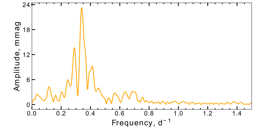
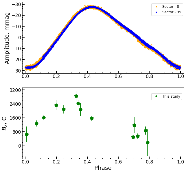
Figure 17: The same as at the Fig. 4 but for HD 86592. Phase diagram is built using the derived rotational period $\emph{P}=2.88657$ for the reduced light curve from the sectors 8 and 35 and for $<B_{\rm z}>$ DAO longitudinal magnetic field measurements(green pentagons).

We carried out analysis of eight Ap stars with the purpose to determine rotation periods from the recently conducted observations with the NASA TESS space telescope and confirm the existence of rotational modulation by comparing phased light curve with the magnetic field measurements phased, with the same period. Thus we have collected all available data for each star from the MAST database up to 50 sectors. We have also collected all available measurements of the mean longitudinal magnetic field $\langle B_{\rm z}\rangle$ for each star (see Table 3), and phased them according to the derived period. Based on the obtained data and the detrended light curves one can admit that the periods derived in this study coincide with those previously mentioned in the literature (see Fig. 18). Nevertheless in most cases, our results are obtained with a much higher precision provided by much larger timescale of analyzed data.

To illustrate the diversity of the global stellar parameters we built Hertzsprung Russell (see top panel of Fig. 19) and Kiel (see bottom panel of Fig. 19) diagrams for 7 targets from our sample by using their derived values of effective temperature and luminosity from Geneva and Strömgren-Crawford photometry and $\log{g}$ from the analysis of Balmer line profiles. We used evolutionary curves of solar metallicity $Z=0.014$ without rotation for stars with 1.5-5.0 $M_{\sun}$ (Bressan et al., 2012), also $\log{g}$ for evolutionary curves were calculated by using formulae derived by Netopil et al. (2017). HD 77314 was not included in the HR diagram and HD 10840 was not included in the Kiel diagram because of absence of observational data required to derive stellar parameters used to build these diagrams. Nevertheless, position of studied stars on these diagrams is consistent with evolutionary tracks of (Bressan et al., 2012) calculated for the same stellar mass, with exception of HD 22920 shifted towards a lower mass level in the Kiel diagram (see Fig 19).

Strong dipolar magnetic fields of fossil origin influence rotational rate in massive, hot OB type stars and causes a loss of angular momentum. Keszthelyi et al. (2020) studied evolutionary models of magnetic stars with dipolar magnetic fields, implementing a magnetic braking formula calibrated from the magnetohydrodynamic simulation (Ud-Doula et al., 2009). The derived evolutionary model that accounts for magnetic braking was tested on the experimental measurements (Shultz et al., 2018) and exhibits rotational spin down of Bp stars. Therefore, we aspire to test whether the ages and periods determined in this study are consistent with those derived for a much larger sample. We used an extensive sample of 100 objects to look for a relation between the fractional main-sequence age ${\tau}_{\mathrm{TAMS}}$ and the rotational rate $v_{\rm eq}/v_{\rm crit}$ by employing data from the studies of rotational properties of ApBp stars by Sikora et al. (2019a, b) (45 objects) and by Shultz et al. (2018, 2019) (48 objects), plus seven stars from this study for which we derived their age (see Tab. 2). Fractional main-sequence ages ${\tau}_{\mathrm{TAMS}}$ for the objects from this study were derived from evolutionary tracks provided by Bressan et al. (2012). Fig. 20 presents a dependence of the rotational period (top panel) and v$\sin{i}$ (bottom panel) on the fractional main-sequence age. While the derived periods of stellar rotation seem to increase with the fractional age (see top panel of Fig. 20), the measured values of v$\sin{i}$ show a tendency to decrease with ${\tau}_{\mathrm{TAMS}}$ (see bottom panel of Fig. 20). These data argue in favour of loss of the angular momentum by the magnetic ApBp stars with their age even if some targets from our sample possess different rotational periods at the similar ${\tau}_{\mathrm{TAMS}}$.

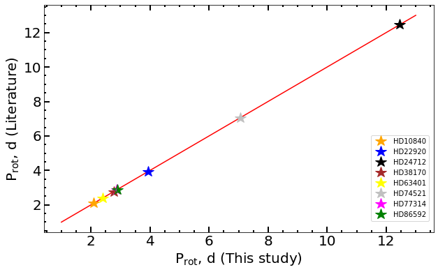
Figure 18: P${}_{\textrm{rot}}$ presented in this study vs P${}_{\textrm{rot}}$ extracted from literature (see Table 1). Red solid line of $x=y$ represents consistency of derived results. Uncertainties are smaller than the used symbols considering the high precision of period estimates.

A dependence of the critical rotational fraction $v_{\rm eq}/v_{\rm crit}$ on the fractional age of studied object at the main sequence ${\tau}_{\mathrm{TAMS}}$ is presented in Fig. 21. Based on the available stellar parameters we determined $v_{\rm eq}/v_{\rm crit}$ for every star in the sample (see Equation 5). This figure shows clearly a decrease of the critical rotational fraction $v_{\rm eq}/v_{\rm crit}$ with the fractional age. The obtained value of the slope stands at -12.0$\pm$ 3.4 which appears to be statistically significant at the 3 $\sigma$-level. We have presented the prediction interval that describes deviation of our estimates of rotational rates from their least square linear approximation. The data may overcome the confidence interval (Cosma, 2019), nevertheless, in our case, only HD 38170 and HD 24712 deviate further from the confidence interval (see pink area in Fig. 21) which proves that the distribution of rotation in our sample is consistent with that observed in the broader population of ApBp stars. The derived decrease of the ratio $v_{\rm eq}/v_{\rm crit}$ with the fractional age seems to be statistically significant (though does not explain much of variation of the data) with the values $p<0.05$ and ${R}^{2}$ = 0.12, and means that younger magnetic ApBp stars rotate faster than older ones on the main sequence.

Our finding is in a good agreement with the works of Abt (1979) and Wolff (1981) arguing that the magnetic ApBp stars start losing their angular momentum after they reach the main sequence. Recent studies of Shultz et al. (2019) have confirmed a slow down of stellar rotation of early Bp stars with age and demonstrated that a sample of Ap stars Sikora et al. (2019a, b) behave in a similar fashion, which is associated with magnetospheric braking.

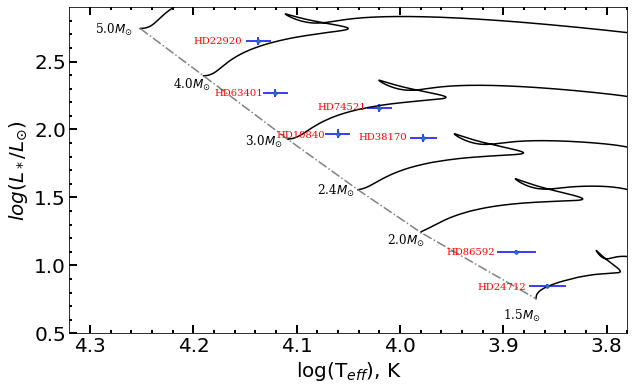
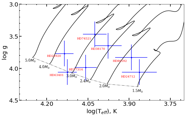
Figure 19: Hertzsprung–Russell diagram (top panel) and Kiel diagram (bottom panel) built for 7 stars from the studied sample. Evolutionary tracks are calculated for stars of 1.5-5.0 $M_{\sun}$ assuming solar metallicity without rotation (the continuous lines) starting from the zero age main sequence (dotted line) (Bressan et al., 2012)

A similar increase of rotational period for ApBp stars with their MS age has been found by Kochukhov & Bagnulo (2006) from the analysis of a sample of 194 objects. This trend appears to be significant for the massive CP stars ($M_{\star}>2M_{\sun}$) and for the low mass objects ($M_{\star}\leq 2M_{\sun}$) which is consistent with our results (see top panel in Fig. 20). Kochukhov & Bagnulo (2006) have reported that for the ApBp stars with $M_{\star}>3M_{\sun}$ the observed increase of rotational period can be explained by the changes of the moment of inertia, while for the group ApBp stars with masses withing $2M_{\sun}<M_{\star}\leq 3M_{\sun}$ this trend may be partially caused by the loss of the angular momentum. Similar results for the massive CP stars ($M_{\star}>3M_{\sun}$) have been also obtained by Hubrig et al. (2007). During investigation of an extensive sample of CP2 and CP4 stars, Netopil et al. (2017) deduced that the angular momentum of CP stars is conserved throughout their main sequence life. These authors noted however that the theoretical change of period with surface gravity $\log{g}$, which is used as the evolutionary parameter (North, 1998), is moderate and cannot account for the significant distribution of rotational periods observed in ApBp stars, especially for the most slowly rotating ones which is consistent with the results of Kochukhov & Bagnulo (2006). Netopil et al. (2017) emphasized that the very-slowly rotating ApBp stars and most of the slowly rotating ApBp stars possess a relatively strong magnetic field implying the crucial role of magnetic field in the slowing-down the rotation of these objects.

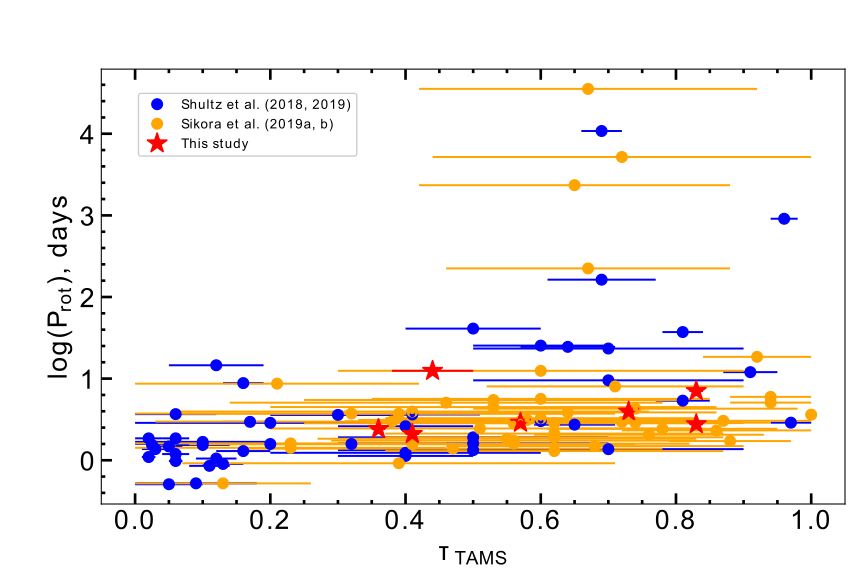
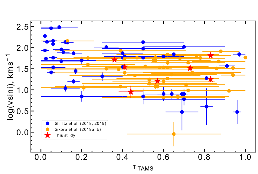
Figure 20: Rotational period (upper panel) and v$\sin{i}$ (lower panel) as a function of fractional age for the sample selected for this study (red stars, see Tab. 2) and for the samples of ApBp stars analysed by Sikora et al. (2019a, b) (orange filled circles) and Shultz et al. (2018, 2019) (blue filled circles).

5 Summary

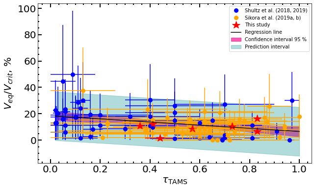
Figure 21: Rotational rates $v_{\rm eq}/v_{\rm crit}$ as a function of fractional age for the seven studied stars (red stars, see Tab.2) and for the ApBp stars reported in Sikora et al. (2019a, b) (orange filled circles) and Shultz et al. (2018, 2019) (blue filled circles).

In this paper, we aimed to test the detrending methods applied to the light curves with rotational modulation provided by TESS for a sample of magnetic ApBp stars with a fairly wide range of global stellar parameters (see Tables 1 & 2). One of our selected targets, HD 24712, does show high-overtone stellar pulsations of roAp type. Discrete Fourier transform of the detrended light curves and available measurements of the mean longitudinal magnetic field (see Table 3) allowed us to derive with high-precision periods of stellar rotation for the selected targets, which are in a good accordance with the previously published data (see. Section 3). Analysis of the stellar global parameters derived from the fitting of Balmer line profiles (see Tables 1) and from the Strömgren-Crawford photometry (see Tables 2) in combination with the analysis of data from Sikora et al. (2019a, b) and Shultz et al. (2018, 2019) resulted in detection of clear decrease of the rotational rate $v_{\rm eq}/v_{\rm crit}$ with the fractional main-sequence age ${\tau}_{\mathrm{TAMS}}$ (see Fig. 21) indicating the loss of angular momentum of ApBp stars with their evolution on the main sequence (Abt, 1979; Wolff, 1981). Considering that our sample contains a considerable number of intermediate mass ApBp stars the found indications of the angular momentum loss are consistent with the arguments for a such possibility expressed by Kochukhov & Bagnulo (2006) and Netopil et al. (2017). The sample analysed in this study includes 100 ApBp stars and is smaller comparing to the samples used by the aforementioned two groups (Kochukhov & Bagnulo, 2006; Netopil et al., 2017). As a part of MOBSTER collaboration we aim to verify our result by expanding significantly the sample of magnetic CP stars with rotational modulation towards low and intermediate mass ($M_{\star}\leq 3M_{\sun}$) objects by using the photometric data obtained from TESS and hopefully from the space telescope PLATO as well.

Data Availability Statement

The data underlying this article are available in the article and in its online supplementary material. The TESS data were extracted from the MAST archive https://archive.stsci.edu. ESPaDOnS spectra used in this article are available at the CFHT archive maintained by the CADC https://www.cadc-ccda.hia-iha.nrc-cnrc.gc.ca/en/cfht.

Appendix A Magnetic field measurements

Table 3: Mean longitudinal magnetic field measurements for eight ApBp stars for this study.

Name (HD)	Epoch of	BJD	$\langle B_{\rm z}\rangle$ G	BJD	$\langle B_{\rm z}\rangle$ G	BJD	$\langle B_{\rm z}\rangle$ G
	zero phase
10840	2458323.56575	Bagnulo et al. (2015)
		2453184.834907	-174$\pm$42
22920	2458409.05852	Borra et al. (1983)		Shultz et al. (2022) (NARVAL)		Shultz et al. (2022) (ESPaDOnS)
		2443736.889	380$\pm$140	2458395.67899	487.13 $\pm$ 22.66	2456557.94247	230.78 $\pm$ 11.64
		2443737.877	200$\pm$120	2458386.64070	148.42 $\pm$ 17.39	2456560.95704	481.11 $\pm$ 12.22
		2443738.847	185$\pm$185	2458387.67402	463.73 $\pm$ 19.67	2456675.70610	451.58 $\pm$ 14.66
		2443740.864	360$\pm$180	2458389.66201	188.29 $\pm$ 13.15	2457437.76397	383.64 $\pm$ 15.52
		Mathys & Hubrig (1997)
		2448847.874	351$\pm$162
24712	2458441.95096	Ryabchikova et al. (1997)		Leone et al. (2000)		Rusomarov et al. (2013)
		2445534.924	1440 $\pm$ 170	2451115.558	540$\pm$335	2455200.719667	742 $\pm$ 6
		2445535.919	1620 $\pm$ 170	2451117.540	530$\pm$125	2455201.735957	946 $\pm$ 7
		2445537.907	810 $\pm$ 240	2451118.528	780$\pm$210	2455202.661397	1064 $\pm$ 7
		2445540.929	590 $\pm$ 190	2451119.522	400$\pm$360	2455203.670667	1059 $\pm$ 6
		2445541.912	500 $\pm$ 140	2451120.514	-180$\pm$120	2455204.656307	912 $\pm$ 6
		2445543.916	690 $\pm$ 260	2451121.520	-225$\pm$220	2455205.681177	720 $\pm$6
		2445544.908	1000$\pm$ 150	2451215.301	355$\pm$530	2455206.656887	512 $\pm$ 5
				2451238.257	550$\pm$460	2455209.652957	219 $\pm$ 3
		Mathys (1994)		Wade et al. (2000)		2455210.670757	305 $\pm$ 4
		2447189.549	212$\pm$202	2450857.334	610$\pm$ 43	2455211.669147	465 $\pm$ 5
		2447190.529	709$\pm$236	2451192.316	1043$\pm$ 58	2455212.667537	640 $\pm$ 6
		This study (ESPaDOnS)		2451193.421	653$\pm$ 86	2455213.671667	837 $\pm$ 6
		2456559.958	798 $\pm$ 20	2451197.362	172$\pm$ 42	2455421.896510	251 $\pm$ 3
		2456560.973	897 $\pm$ 25			2455606.535706	321 $\pm$ 4
						2455607.554866	223 $\pm$ 3
38170	2458438.05343	David-Uraz et al. (2021)
		2458741.145913	-6$\pm$25
		2458743.146673	105$\pm$14
63401	2458491.71207	Bagnulo et al. (2015)		This study (ESPaDOnS)
		2452678.529602	-589$\pm$53	2455521.6568	308$\pm$65
		2453002.556151	153$\pm$95	2457108.2348	-109$\pm$58
		2453004.731597	-414$\pm$101	2457109.2598	396$\pm$60
		2453399.628828	322$\pm$55	2457110.2218	339$\pm$49
				2457111.2948	-47$\pm$23
				2457112.2818	338$\pm$54
				2457113.2938	-400$\pm$70
74521	2458491.78360	Bohlender et al. (1993)		Mathys (1994)		Leone (2007)
		2446834.679	770$\pm$140	2446894.528	967$\pm$121	2453718.717	1032$\pm$ 30
		2446835.715	640$\pm$140	2446895.485	850$\pm$128	2453719.710	794$\pm$ 28
		2446836.750	580$\pm$140	2447279.531	398$\pm$190	This study (ESPaDOnS)
		2446837.703	500$\pm$160	2447280.529	418$\pm$156	2457435.932	528$\pm$ 23
		2446894.616	200$\pm$300	2447281.465	603$\pm$107	2458437.606	541$\pm$ 25
						2458457.643	538$\pm$ 26
77314	2458519.36909	This study (dimaPol)
		2455261.87680	-159$\pm$263
		2455264.79807	259$\pm$220
		2455580.93253	35$\pm$205
		2456678.93416	-291$\pm$167
86592	2458573.33597	This study (dimaPol)		This study (dimaPol)		This study (dimaPol)
		2456355.84065	187$\pm$755	2457088.84276	551$\pm$159	2458561.81803	664$\pm$447
		2456992.07270	2323$\pm$297	2457089.84700	1281$\pm$174	2458562.81450	2080$\pm$359
		2456995.09549	2098$\pm$247	2457090.87518	1579$\pm$143	2458563.81851	1190$\pm$449
		2457084.84742	2421$\pm$181	2457465.83889	2852$\pm$294	2458569.79994	873$\pm$238
		2457085.87101	505$\pm$248	2457476.78068	1613$\pm$121

References

- Abt (1979) Abt H. A., 1979, ApJ, 230, 485
- Abt & Morrell (1995) Abt H. A., Morrell N. I., 1995, ApJS, 99, 135
- Alecian & Stift (2010) Alecian G., Stift M. J., 2010, A&A, 516, A53
- Alecian & Stift (2019) Alecian G., Stift M. J., 2019, MNRAS, 482, 4519
- Alecian & Stift (2021) Alecian G., Stift M. J., 2021, MNRAS, 504, 1370
- Aurière et al. (2007) Aurière M., et al., 2007, A&A, 475, 1053
- Babel & North (1997) Babel J., North P., 1997, A&A, 325, 195
- Bagnulo et al. (1995) Bagnulo S., Landi Degl’Innocenti E., Landolfi M., Leroy J. L., 1995, A&A, 295, 459
- Bagnulo et al. (2002) Bagnulo S., Szeifert T., Wade G. A., Landstreet J. D., Mathys G., 2002, A&A, 389, 191
- Bagnulo et al. (2015) Bagnulo S., Fossati L., Landstreet J. D., Izzo C., 2015, A&A, 583, A115
- Bailey & Landstreet (2013) Bailey J. D., Landstreet J. D., 2013, A&A, 551, A30
- Bailey et al. (2014) Bailey J. D., Landstreet J. D., Bagnulo S., 2014, A&A, 561, A147
- Bartholdi (1988) Bartholdi P., 1988, in Halbwachs J. L., Jasniewicz G., Egret D., eds, Détection et Classification des Étoiles Variables. pp 77–83
- Bernhard et al. (2020) Bernhard K., Hümmerich S., Paunzen E., 2020, MNRAS, 493, 3293
- Bevington (1969) Bevington P. R., 1969, Data reduction and error analysis for the physical sciences. McGraw-Hill (New York)
- Bohlender et al. (1993) Bohlender D. A., Landstreet J. D., Thompson I. B., 1993, A&A, 269, 355
- Borra et al. (1983) Borra E. F., Landstreet J. D., Thompson I., 1983, ApJS, 53, 151
- Bowman et al. (2018) Bowman D. M., Buysschaert B., Neiner C., Pápics P. I., Oksala M. E., Aerts C., 2018, A&A, 616, A77
- Bressan et al. (2012) Bressan A., Marigo P., Girardi L., Salasnich B., Dal Cero C., Rubele S., Nanni A., 2012, MNRAS, 427, 127
- Buysschaert et al. (2018) Buysschaert B., Neiner C., Martin A. J., Aerts C., Bowman D. M., Oksala M. E., Van Reeth T., 2018, MNRAS, 478, 2777
- Bychkov et al. (2003) Bychkov V. D., Bychkova L. V., Madej J., 2003, A&A, 407, 631
- Caldwell et al. (2020) Caldwell D. A., et al., 2020, Research Notes of the American Astronomical Society, 4, 201
- Cannon & Pickering (1993) Cannon A. J., Pickering E. C., 1993, VizieR Online Data Catalog, p. III/135A
- Catanzaro et al. (1999) Catanzaro G., Leone F., Catalano F. A., 1999, A&AS, 134, 211
- Cosma (2019) Cosma R., 2019, The Truth about Linear Regression
- Cowley et al. (1968) Cowley A. P., Cowley C. R., Hiltner W. A., Jaschek M., Jaschek C., 1968, PASP, 80, 746
- Cox (2000) Cox A. N., 2000, Allen’s astrophysical quantities
- Cunha et al. (2019) Cunha M. S., et al., 2019, MNRAS, 487, 3523
- David-Uraz et al. (2021) David-Uraz A., et al., 2021, MNRAS, 504, 4841
- Donati & Collier Cameron (1997) Donati J. F., Collier Cameron A., 1997, MNRAS, 291, 1
- Donati et al. (1997) Donati J. F., Semel M., Carter B. D., Rees D. E., Collier Cameron A., 1997, MNRAS, 291, 658
- Donati et al. (2006) Donati J. F., Catala C., Landstreet J. D., Petit P., 2006, in Casini R., Lites B. W., eds, Astronomical Society of the Pacific Conference Series Vol. 358, Solar Polarization 4. p. 362
- Dukes & Adelman (2018) Dukes Robert J. J., Adelman S. J., 2018, PASP, 130, 044202
- Flower (1996) Flower P. J., 1996, ApJ, 469, 355
- Gangestad et al. (2013) Gangestad J. W., Henning G. A., Persinger R. y. R., Ricker G. R., 2013, arXiv e-prints, p. arXiv:1306.5333
- Georgy et al. (2013) Georgy C., Ekström S., Granada A., Meynet G., Mowlavi N., Eggenberger P., Maeder A., 2013, A&A, 553, A24
- Glagolevskij (2007) Glagolevskij Y. V., 2007, Astrophysical Bulletin, 62, 244
- Gontcharov (2006) Gontcharov G. A., 2006, Astronomy Letters, 32, 759
- Hauck & Mermilliod (1998) Hauck B., Mermilliod M., 1998, A&AS, 129, 431
- Hauck & North (1982) Hauck B., North P., 1982, A&A, 114, 23
- Hauschildt & Baron (1999) Hauschildt P. H., Baron E., 1999, Journal of Computational and Applied Mathematics, 109, 41
- Hauschildt et al. (1997) Hauschildt P. H., Baron E., Allard F., 1997, ApJ, 483, 390
- Hensberge et al. (1976) Hensberge H., De Loore C., Zuiderwijk E. J., Hammerschlag-Hensberge G., 1976, A&A, 48, 383
- Holdsworth (2021) Holdsworth D. L., 2021, Frontiers in Astronomy and Space Sciences, 8, 31
- Holdsworth et al. (2021) Holdsworth D. L., et al., 2021, MNRAS, 506, 1073
- Houk & Cowley (1975) Houk N., Cowley A. P., 1975, University of Michigan Catalogue of two-dimensional spectral types for the HD stars. Volume I. Declinations -90_ to -53_°0.
- Houk & Smith-Moore (1988) Houk N., Smith-Moore M., 1988, Michigan Catalogue of Two-dimensional Spectral Types for the HD Stars. Volume 4, Declinations -26°.0 to -12°.0.
- Houk & Swift (1999) Houk N., Swift C., 1999, Michigan Spectral Survey, 5, 0
- Hubrig et al. (2007) Hubrig S., North P., Schöller M., 2007, Astronomische Nachrichten, 328, 475
- Husser et al. (2013) Husser T. O., Wende-von Berg S., Dreizler S., Homeier D., Reiners A., Barman T., Hauschildt P. H., 2013, A&A, 553, A6
- Jenkins et al. (2016) Jenkins J. M., et al., 2016, in Chiozzi G., Guzman J. C., eds, Society of Photo-Optical Instrumentation Engineers (SPIE) Conference Series Vol. 9913, Software and Cyberinfrastructure for Astronomy IV. p. 99133E, doi:10.1117/12.2233418
- Keszthelyi et al. (2020) Keszthelyi Z., et al., 2020, MNRAS, 493, 518
- Khalack (2018) Khalack V., 2018, MNRAS, 477, 882
- Khalack & LeBlanc (2015) Khalack V., LeBlanc F., 2015, AJ, 150, 2
- Khalack & Poitras (2015) Khalack V., Poitras P., 2015, in New Windows on Massive Stars. pp 383–384
- Khalack et al. (2017) Khalack V., Gallant G., Thibeault C., 2017, MNRAS, 471, 926
- Khalack et al. (2019) Khalack V., et al., 2019, MNRAS, 490, 2102
- Khalack et al. (2020) Khalack V., LeBlanc F., Kobzar O., 2020, in Stellar Magnetism: A Workshop in Honour of the Career and Contributions of John D. Landstreet. pp 201–208 (arXiv:2003.02936)
- Kobzar et al. (2020) Kobzar O., et al., 2020, in Wade G., Alecian E., Bohlender D., Sigut A., eds, Vol. 11, Stellar Magnetism: A Workshop in Honour of the Career and Contributions of John D. Landstreet. pp 214–218 (arXiv:2003.05337)
- Kochukhov & Bagnulo (2006) Kochukhov O., Bagnulo S., 2006, A&A, 450, 763
- Kochukhov & Piskunov (2002) Kochukhov O., Piskunov N., 2002, A&A, 388, 868
- Kochukhov et al. (2010) Kochukhov O., Makaganiuk V., Piskunov N., 2010, A&A, 524, A5
- Kochukhov et al. (2011) Kochukhov O., Rivinius T., Oksala M. E., Romanyuk I., 2011, in Neiner C., Wade G., Meynet G., Peters G., eds, Vol. 272, Active OB Stars: Structure, Evolution, Mass Loss, and Critical Limits. pp 166–171, doi:10.1017/S1743921311010192
- Kochukhov et al. (2018) Kochukhov O., Johnston C., Alecian E., Wade G. A., BinaMIcS Collaboration 2018, MNRAS, 478, 1749
- Kochukhov et al. (2019) Kochukhov O., Shultz M., Neiner C., 2019, A&A, 621, A47
- Kordopatis et al. (2013) Kordopatis G., et al., 2013, AJ, 146, 134
- Krtička et al. (2015) Krtička J., Mikulášek Z., Lüftinger T., Jagelka M., 2015, A&A, 576, A82
- Kurtz (1978) Kurtz D. W., 1978, Information Bulletin on Variable Stars, 1436, 1
- Kurtz (1981) Kurtz D. W., 1981, Information Bulletin on Variable Stars, 1915, 1
- Kurtz & Marang (1987) Kurtz D. W., Marang F., 1987, MNRAS, 229, 285
- Landstreet (1982) Landstreet J. D., 1982, ApJ, 258, 639
- Landstreet et al. (2007) Landstreet J. D., Bagnulo S., Andretta V., Fossati L., Mason E., Silaj J., Wade G. A., 2007, A&A, 470, 685
- LeBlanc et al. (2015) LeBlanc F., Khalack V., Yameogo B., Thibeault C., Gallant I., 2015, MNRAS, 453, 3766
- Lenz & Breger (2005) Lenz P., Breger M., 2005, Communications in Asteroseismology, 146, 53
- Leone (2007) Leone F., 2007, MNRAS, 382, 1690
- Leone & Manfre (1996) Leone F., Manfre M., 1996, A&A, 315, 526
- Leone et al. (2000) Leone F., Catanzaro G., Catalano S., 2000, A&A, 355, 315
- Levato et al. (1996) Levato H., Malaroda S., Morrell N., Solivella G., Grosso M., 1996, A&AS, 118, 231
- Mathys (1991) Mathys G., 1991, A&AS, 89, 121
- Mathys (1994) Mathys G., 1994, A&AS, 108, 547
- Mathys (1995) Mathys G., 1995, A&A, 293, 746
- Mathys (2017) Mathys G., 2017, A&A, 601, A14
- Mathys & Hubrig (1997) Mathys G., Hubrig S., 1997, A&AS, 124, 475
- Michaud (1970) Michaud G., 1970, ApJ, 160, 641
- Michaud et al. (2015) Michaud G., Alecian G., Richer J., 2015, Atomic Diffusion in Stars, doi:10.1007/978-3-319-19854-5.
- Monin et al. (2015) Monin D., Bohlender D., Hardy T., Saddlemyer L., 2015, in Nagendra K. N., Bagnulo S., Centeno R., Jesús Martínez González M., eds, None Vol. 305, Polarimetry. pp 191–194, doi:10.1017/S1743921315004755
- Napiwotzki et al. (1993) Napiwotzki R., Schoenberner D., Wenske V., 1993, A&A, 268, 653
- Napiwotzki et al. (2004) Napiwotzki R., et al., 2004, in Hilditch R. W., Hensberge H., Pavlovski K., eds, Astronomical Society of the Pacific Conference Series Vol. 318, Spectroscopically and Spatially Resolving the Components of the Close Binary Stars. pp 402–410 (arXiv:astro-ph/0403595)
- Ndiaye et al. (2018) Ndiaye M. L., LeBlanc F., Khalack V., 2018, MNRAS, 477, 3390
- Neiner et al. (2015) Neiner C., Mathis S., Alecian E., Emeriau C., Grunhut J., BinaMIcS MiMeS Collaborations 2015, in Polarimetry. pp 61–66 (arXiv:1502.00226), doi:10.1017/S1743921315004524
- Netopil et al. (2008) Netopil M., Paunzen E., Maitzen H. M., North P., Hubrig S., 2008, A&A, 491, 545
- Netopil et al. (2017) Netopil M., Paunzen E., Hümmerich S., Bernhard K., 2017, MNRAS, 468, 2745
- North (1998) North P., 1998, A&A, 334, 181
- Paunzen (2015) Paunzen E., 2015, A&A, 580, A23
- Petit & Wade (2012) Petit V., Wade G. A., 2012, MNRAS, 420, 773
- Piskunov & Kochukhov (2002) Piskunov N., Kochukhov O., 2002, A&A, 381, 736
- Preston (1972) Preston G. W., 1972, ApJ, 175, 465
- Preston (1974) Preston G. W., 1974, ARA&A, 12, 257
- Raskin et al. (2011) Raskin G., et al., 2011, A&A, 526, A69
- Renson & Manfroid (1992) Renson P., Manfroid J., 1992, A&A, 263, 161
- Ricker et al. (2015) Ricker G. R., et al., 2015, Journal of Astronomical Telescopes, Instruments, and Systems, 1, 014003
- Royer et al. (2002) Royer F., Grenier S., Baylac M. O., Gómez A. E., Zorec J., 2002, A&A, 393, 897
- Rufener (1988) Rufener F., 1988, Catalogue of stars measured in the Geneva Observatory photometric system : 4 : 1988
- Rusomarov et al. (2013) Rusomarov N., et al., 2013, A&A, 558, A8
- Rusomarov et al. (2015) Rusomarov N., Kochukhov O., Ryabchikova T., Piskunov N., 2015, A&A, 573, A123
- Ryabchikova et al. (1997) Ryabchikova T. A., Landstreet J. D., Gelbmann M. J., Bolgova G. T., Tsymbal V. V., Weiss W. W., 1997, A&A, 327, 1137
- Ryabchikova et al. (2007) Ryabchikova T., et al., 2007, A&A, 462, 1103
- Samus’ et al. (2017) Samus’ N. N., Kazarovets E. V., Durlevich O. V., Kireeva N. N., Pastukhova E. N., 2017, Astronomy Reports, 61, 80
- Shultz et al. (2018) Shultz M. E., et al., 2018, MNRAS, 475, 5144
- Shultz et al. (2019) Shultz M. E., et al., 2019, MNRAS, 490, 274
- Shultz et al. (2022) Shultz M. E., et al., 2022, arXiv e-prints, p. arXiv:2201.05512
- Sichevskij (2017) Sichevskij S. G., 2017, Astronomy Reports, 61, 193
- Sikora et al. (2019a) Sikora J., Wade G. A., Power J., Neiner C., 2019a, MNRAS, 483, 2300
- Sikora et al. (2019b) Sikora J., Wade G. A., Power J., Neiner C., 2019b, MNRAS, 483, 3127
- Sikora et al. (2019c) Sikora J., et al., 2019c, MNRAS, 487, 4695
- Silvester et al. (2017) Silvester J., Kochukhov O., Rusomarov N., Wade G. A., 2017, MNRAS, 471, 962
- Stassun et al. (2018) Stassun K. G., et al., 2018, AJ, 156, 102
- Stassun et al. (2019) Stassun K. G., et al., 2019, VizieR Online Data Catalog, p. J/AJ/156/102
- Stepien (1968) Stepien K., 1968, ApJ, 154, 945
- Strömgren (1966) Strömgren B., 1966, ARA&A, 4, 433
- Torres (2010) Torres G., 2010, AJ, 140, 1158
- Ud-Doula et al. (2009) Ud-Doula A., Owocki S. P., Townsend R. H. D., 2009, MNRAS, 392, 1022
- Wade et al. (2000) Wade G. A., Donati J. F., Landstreet J. D., Shorlin S. L. S., 2000, MNRAS, 313, 851
- Wade et al. (2016) Wade G. A., et al., 2016, MNRAS, 456, 2
- Watson et al. (2006) Watson C. L., Henden A. A., Price A., 2006, Society for Astronomical Sciences Annual Symposium, 25, 47
- Wolff (1981) Wolff S. C., 1981, ApJ, 244, 221
- Wraight et al. (2012) Wraight K. T., Fossati L., Netopil M., Paunzen E., Rode-Paunzen M., Bewsher D., Norton A. J., White G. J., 2012, MNRAS, 420, 757
- Zorec & Royer (2012) Zorec J., Royer F., 2012, A&A, 537, A120