Bayesian Parameterization of Continuum Battery Models from Featurized Electrochemical Measurements Considering Noise
Zusammenfassung
keywords:
Introduction
Batteries are essential for the decarbonization of heavy industry and electricity supply. With their high specific energy density, Li-ion batteries are crucial for efficiently electrifying personal transport, freight transport, and aviation. These applications require materials with optimal energy density, efficiency, and safety. Theoretical electrochemists use physics-based continuum battery models 1 to aid in the search for optimal materials. Physics-based models can predict battery operation and failure modes from material properties rather than artificial fit parameters 2. The parameterization of these models is crucial to verify and enhance them. Since the amount of data grows faster than experts can analyze it, such parameterization should be automated. Parameterization of physics-based battery models may reveal the material properties of a battery from non-destructive measurements. Non-destructive measurements are essential since specific material properties change during the lifetime of a battery. Ageing effects include the formation of a Solid-Electrolyte Interphace (SEI) 3 and Lithium plating 4. Tracking these mechanisms is imperative for modelling them. Non-destructive measurements of physical battery parameters usually require special experimental setups. Examples are the Galvanostatic Intermittent Titration Technique (GITT) to measure transport properties 5, Staircase GITT to measure reaction kinetics 6, Electrochemical Impedance Spectroscopy (EIS) to measure the electrode-electrolyte interfacial kinetics 7, or Nuclear Magnetic Resonance (NMR) to measure ionic transport in the electrolyte 8, 9. Associated analytical formulas may extract the physical properties of a battery. However, these formulas seldomly adapt well to slight variations in operating conditions, as demonstrated by Horner et al. 10 in the case of GITT. This traditional approach often requires some manual fine-tuning. Recent efforts are devoted to developing automated parameterization methods. Automated algorithms based on physics-based models can cope with less handpicked input. In this case, the task is to match the simulated model to the experimental data. Usually, this will involve repeated model evaluations by an optimization algorithm. Commonly used optimizers for battery models are Least Squares 11, Monte Carlo 12, and Genetic Algorithms 13, 14. All of these have a stochastical element for efficiency but do not give error bars for their parameterizations. Bayesian algorithms such as Kalman Filters 15, 16 and Markov-Chain Monte Carlo 17 simultaneously provide the optimal parameters and their uncertainty. Another method of adding error bars is to repeat the parameterization with artificial noise in the data that mimics the original noise 18. For best results, multiple approaches to parameterization have to be combined 19. Model substitution is a technique primarily employed by data scientists to accelerate parameterization. There, a Neural Network or other stochastical classifier gets fitted to a physics-based model and is then used instead in an optimizer 20, 21, 22, 23. Imaging techniques also give essential input parameters for spatially resolved simulations and have to concern themselves with the uncertainty propagation from imaging to simulation outcome 24, 25, 26, 27, 28. The State-of-Health estimation of degradation modes may also benefit from a physical understanding of the degradation processes involved 29. Bayesian algorithms directly match model simulations to experimental data and to the uncertainty in that data. The considerable noise in battery characterization measurements is thus well handled in Bayesian algorithms. To the best of our knowledge, only two distinct types of Bayesian algorithms are in use for the simultaneous estimation of parameters of continuum battery models and their uncertainty. On the one hand, there are Dual Kalman Filters (DKF) 15, 16, which estimate the state of the simulated battery over time and can also optimize the model parameters. The high flexibility of DKF estimations has a drawback: DKFs have to be tuned perfectly and require an increased effort for integration with the model simulation. Otherwise, their results are technically correct but physically unreasonable. On the other hand, there are Markov-Chain Monte Carlo (MCMC) algorithms 17, which run tens of thousands of simulations to find the one that fits the experiment the best. Stability is thus enhanced at the cost of run-time, so only simplified battery models that simulate in milliseconds are currently used 17, 11. Uncertainty Quantification (UQ), i.e., estimation of the precision of parameter fits, is a significant advantage of Bayesian algorithms. Predicting battery performance and failure modes relies heavily on the accuracy of the model parameters. However, the precision with which a parameter is identifiable in a given measurement gets often neglected 30, 31, 32. In other words, it is then doubtful that the measurement uniquely identifies the fit parameters. For example, Escalante et al. 33 apply Bayesian inference to charge-discharge cycles and find that they are barely suitable for battery model parameterization. Especially in the presented case of a partial Differential-Algebraic Equation model, parameterizing it is an „inverse problem“. „Inverse problems“ are ill-posed in that they admit a family of infinitely many approximate solutions rather than one unambiguous one, as „direct problems“ do. With Bayesian algorithms, these many solutions can be ranked systematically by their assigned probabilities and parameter interdependencies can be formally analyzed via their correlations. Still, it is important to keep the number of estimated model parameters small. Systematic model parameterizations 11, 34, 35, 13 are crucial for the reproducibility and transferability of the results. Further theoretical and experimental developments may build upon such reusable prior work. This article introduces a new Bayesian algorithm, called EP-BOLFI, for the automated estimation of model parameters by applying it to continuum battery models. Our algorithm requires one order of magnitude fewer simulations and is more stable than the MCMC approach, requiring only a consumer-grade computer. Our algorithm is independent of the battery model and the experiment, so different battery models can be examined quickly for identifiability from any measurement. Battery modelling experts can input their expertise to improve the parameterization by segmenting the data into „features“. Other than taking segments of the raw data, using the parameters of fitting functions on the data as features can improve weighting of the information contained in the data. While we deliberately do not automate the feature selection, it is possible to automatically select from a set of candidate fitting functions 36. We briefly show the battery model’s equations we apply our algorithm to as an example in Subsection Physics-Based Battery Models. We give a short introduction to the Bayesian idea in general in Subsection Introduction to the Bayesian Principle (for Likelihood-Free Inference). A deeper understanding of the two Bayesian algorithms we use follows, namely Expectation Propagation 37 in Subsection Expectation Propagation and a specific Bayesian Optimization implementation 38 in Subsection Bayesian Optimization (for Likelihood-Free Inference). We compare our algorithm with the state of the art in Bayesian parameterization, namely MCMC, in Section Validation of EP-BOLFI performance. The properties of the lithium-ion battery we measured, the selection of the unknown parameters we fit and the setup of the battery model we fit are in Section Experimental. We then show the application of these algorithms to full-cell GITT measurements in Section Results from full-cell GITT data. A discussion of the results of our algorithm follows in Section Discussions. We conclude this paper with our findings in Section Conclusion.Theory
Physics-Based Battery Models
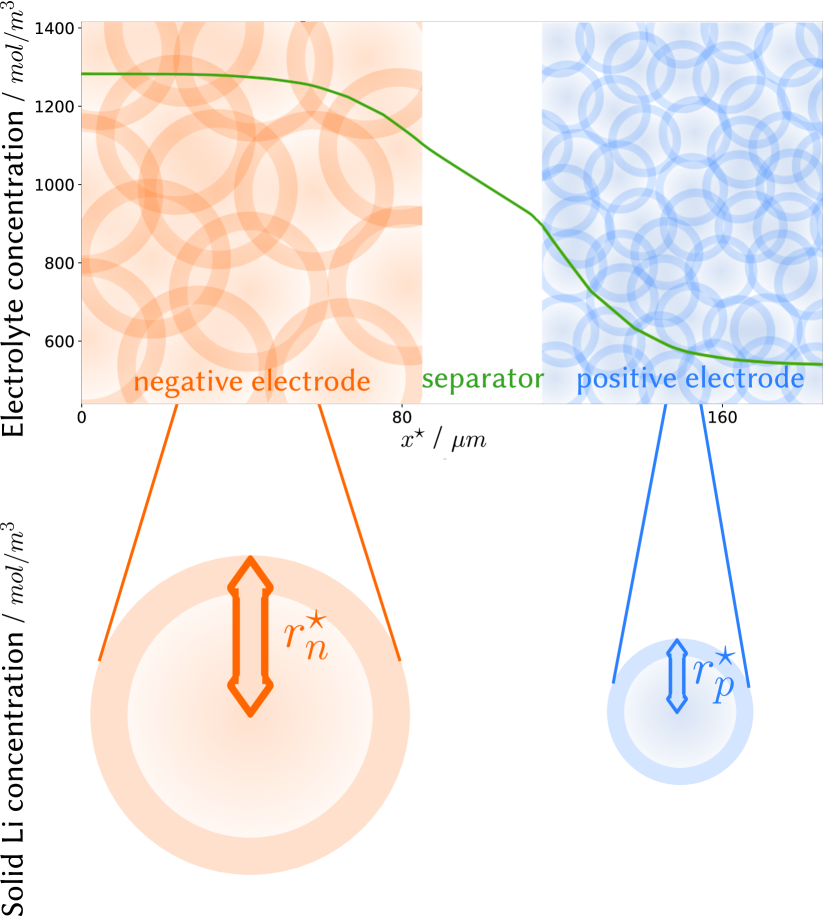 Abbildung 1: Schema of a battery cell as represented by the DFN model in table 1. All particles at the same place in -direction are averaged into one representative particle.
Tabelle 1: 1D+1D physics-based continuum battery model equations
Abbildung 1: Schema of a battery cell as represented by the DFN model in table 1. All particles at the same place in -direction are averaged into one representative particle.
Tabelle 1: 1D+1D physics-based continuum battery model equationsferential-Algebraic Equations (DAE). Solving partial DAEs on a microstructure-resolving 3D grid requires high-performance computers. Volume-averaged 3D model simulations still take a couple of days 39. Hence, volume-averaged 1D+1D models 1 have been developed as a suitable compromise between accuracy and speed. In this paper we will use the Doyle-Fuller-Newman (DFN) 1D+1D model. There are further simplifications down to 1D, especially the Single Particle Model (SPM) and the SPM with electrolyte modification (SPMe) 40. However, we found that these cannot accurately describe the GITT experiments which represent the main example in this article. 1D+1D models 1 represent a battery on the cell level: porous anode, porous separator, and porous cathode. Inside this porous structure, the ionically conducting electrolyte is modelled as a continuum. The electrodes are simplified to a cluster of spherical, homogenous particles in which intercalated lithium diffuses. These representative particles are separated by electrolyte and not in direct contact. 1D+1D models are still too costly to evaluate for parameter identification schemes that require hundreds of thousands of simulations. For example, Aitio et al. 17 instead use an asymptotically simplified model, the Single-Particle Model with electrolyte (SPMe) 40. The SPMe consists of ordinary differential equations (ODE) only. These ODEs simulate in milliseconds, but the SPMe gives inaccurate results at currents over . In table 1 we summarize the common ancestor of all 1D+1D models, the Doyle-Fuller-Newman (DFN) model 41, in a non-dimensionalized form laid out by Marquis et al. 40. Figure 1 visualizes the level of detail the DFN describes: all material properties and dynamics are assumed to be homogenous perpendicular to the line between the current collectors. Along this line, the DFN describes lithium(-ion) concentrations and potentials in the electrodes and the electrolyte. The DFN model parameters are summarized in Table 5 and Table 6. The boundary conditions and initial conditions that complete the DAE system are stated in the SI Section LABEL:SI-sec:boundary_conditions.
Introduction to the Bayesian Principle (for Likelihood-Free Inference)
 Abbildung 2: Monte Carlo algorithm for Bayes’ Theorem. is a placeholder for „data“ and is a placeholder for „model parameters“.
Updating prior knowledge given new evidence: this is the central idea behind any Bayesian algorithm. The preconditioning of estimation problems with prior knowledge enables Bayesian algorithms to require far fewer data points than empirical approaches. Some standard textbooks for Bayesian inference are References 42, 43, 44.
„Probability“ in the Bayesian context describes the level of uncertainty in the data rather than randomness. The result of any Bayesian algorithm is a probability distribution providing a range of estimates with their respective „probabilities“ to be the correct estimate. The estimated probability distribution also includes information about how the estimated model parameters influence the measurement individually and collectively 42, 43, 44.
Here we describe the basic Bayesian algorithm, which we outline in Figure 2. Firstly, transform the prior knowledge about the range of probable model parameters into a probability distribution , called Prior or „belief“. Secondly, take random samples from the Prior and calculate the so-called Likelihood for each parameter sample. The Likelihood represents the „Likelihood“ for each model simulation to match the experimental data. A simple approximation for the Likelihood is a Gaussian distribution with the simulation-experiment agreement as its expectation value and some variance 17. Finally, multiply the Likelihood with the Prior and normalize the result into a probability distribution , called Posterior. The third step is eq. 2, called Bayes’ Theorem. Bayes’ Theorem ensures that the Posterior reasonably updates the prior belief about probable parameter candidates 42, 43, 44,
(2)
In the following, we abbreviate „parameter“ as and „data“ as , as shown in Figure 2. Bayes’ Theorem then reads as .
The performance of a Bayesian algorithm crucially depends on the quality of the Likelihood approximation. A rough approximation of a Likelihood with a Gaussian 17 might lead to slow convergence or wrong estimates. And in the case of 1D+1D models without analytic solutions, a better Likelihood cannot be derived. However, the approximation that the Posterior is Gaussian is usually justified if the estimated parameters are identifiable from the data, given the Central Limit Theorem 42, 43, 44.
Likelihood-Free Inference (LFI), also called Approximate Bayes-
Abbildung 2: Monte Carlo algorithm for Bayes’ Theorem. is a placeholder for „data“ and is a placeholder for „model parameters“.
Updating prior knowledge given new evidence: this is the central idea behind any Bayesian algorithm. The preconditioning of estimation problems with prior knowledge enables Bayesian algorithms to require far fewer data points than empirical approaches. Some standard textbooks for Bayesian inference are References 42, 43, 44.
„Probability“ in the Bayesian context describes the level of uncertainty in the data rather than randomness. The result of any Bayesian algorithm is a probability distribution providing a range of estimates with their respective „probabilities“ to be the correct estimate. The estimated probability distribution also includes information about how the estimated model parameters influence the measurement individually and collectively 42, 43, 44.
Here we describe the basic Bayesian algorithm, which we outline in Figure 2. Firstly, transform the prior knowledge about the range of probable model parameters into a probability distribution , called Prior or „belief“. Secondly, take random samples from the Prior and calculate the so-called Likelihood for each parameter sample. The Likelihood represents the „Likelihood“ for each model simulation to match the experimental data. A simple approximation for the Likelihood is a Gaussian distribution with the simulation-experiment agreement as its expectation value and some variance 17. Finally, multiply the Likelihood with the Prior and normalize the result into a probability distribution , called Posterior. The third step is eq. 2, called Bayes’ Theorem. Bayes’ Theorem ensures that the Posterior reasonably updates the prior belief about probable parameter candidates 42, 43, 44,
(2)
In the following, we abbreviate „parameter“ as and „data“ as , as shown in Figure 2. Bayes’ Theorem then reads as .
The performance of a Bayesian algorithm crucially depends on the quality of the Likelihood approximation. A rough approximation of a Likelihood with a Gaussian 17 might lead to slow convergence or wrong estimates. And in the case of 1D+1D models without analytic solutions, a better Likelihood cannot be derived. However, the approximation that the Posterior is Gaussian is usually justified if the estimated parameters are identifiable from the data, given the Central Limit Theorem 42, 43, 44.
Likelihood-Free Inference (LFI), also called Approximate Bayes-
ian Computation (ABC), is a class of algorithms that approximate the unknown Likelihood from model evaluations. The shape of the Likelihood in LFI algorithms results from a Machine Learning procedure on simulated data samples, e.g., Cross-Validation 45. Instead of a Likelihood, LFI algorithms only need to know the discrepancy measure between a simulated measurement and an experiment. The added flexibility enables one to try out different models freely 46. In contrast to DKFs, the discrepancy measure in LFI algorithms may encompass the whole experimental data rather than only one point in a time series at a time. The difference to MCMC methods such as the Metropolis-Hastings algorithm used by Aitio et al. 17 is that the quality of parameter guesses is judged by the approximated Likelihood rather than by the Posterior. Using the Posterior like Metropolis-Hastings may result in confirmation bias since it mixes the Prior into evaluating the quality of parameter fits. The following sections present the two LFI algorithms we employ to minimize the required number of model simulations. Despite the improved generality and accuracy of our approach, we achieve a reduction rather than an increase in computational load compared to Metropolis-Hastings.
Expectation Propagation
Expectation Propagation (EP) was developed by Minka in his PhD thesis 47 and later revisited in a paper 48. EP has uses for training neural networks 49, object detection 50, speech recognition 51, and signal processing 52. We present Barthelmé et al.’s adaptation of EP to Likelihood-Free Inference (LFI) 37 using BOLFI as LFI algorithm (see Subsection Bayesian Optimization (for Likelihood-Free Inference) for BOLFI). For further reading, we recommend the general introduction to EP in 53, Chapter 3.6. The great advantage of EP for LFI is splitting the data into multiple segments or discrete features. These features give the sampling algorithm within EP the more straightforward task of matching one part of the data at a time. EP is proven to work accurately and efficiently based on its two core principles. First, the moments of the approximated Posterior converge to the moments of the actual Posterior. Examples of moments for probability distributions are the expectation value and the variance. Formally, moment-matching is only guaranteed if Posteriors get selected from an exponential family. Further details are summarized in the SI Section LABEL:SI-sec:expfam. Second, EP efficiently optimizes multiple measurement parts together by iterating through them. From now on, we call these measurement parts „features“ and denote them with . EP searches the optimal parameter set for each feature in the range of probable candidates for the other features. Examples of possible features range from measurements in time to characteristic values, like decay rates. The user sets up EP with the following two inputs 37. One is a functional definition of the features in simulation and data, which defines the cost function. The other is a Prior , which represents the initial belief for every vector of parameter values and defines the „initial value“ of the Bayesian algorithm. Additionally, one may pre-define the Likelihood sites for each of the features, but for initialization „uninformative Priors“ are appropriate. The EP algorithm then expresses the Posterior as the product of the Prior and each Likelihood site, as shown in eq. 3. (3)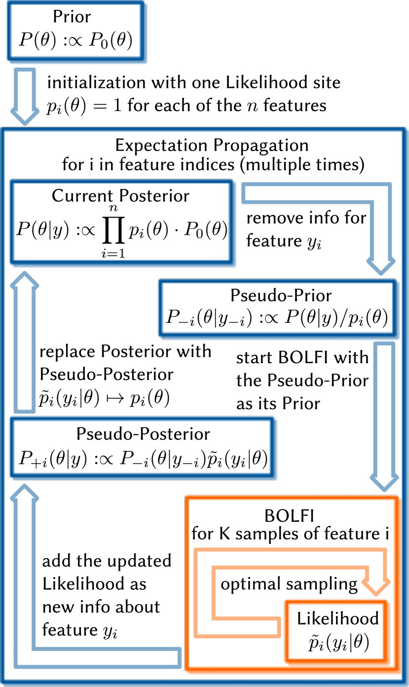 Abbildung 3: Iterative Expectation Propagation (EP) algorithm. Choose a random feature , create a search space by omitting the factor for in , sample that search space to obtain a local Posterior and replace with it. BOLFI is presented in Subsection Bayesian Optimization (for Likelihood-Free Inference) and is our choice for the LFI algorithm inside EP.
The procedure for EP 37 factorizes the simulation and data into individual features. EP then iterates through all features multiple times. For each feature, BOLFI optimizes the model parameters to fit this feature. The result of BOLFI is a more precise probability distribution of the model parameters. EP utilizes this result to update its distribution of probable model parameters for all features. EP uses the new Posterior as input for next feature optimization.
The algorithm of EP 37 iterates through the features of the whole data until a stop criterion is met, as shown in Figure 3. After initialization of the current Posterior with the Prior and the initial Likelihood sites, there are four steps in each iteration. Firstly, produce a „Pseudo-Prior“ by omitting the corresponding Likelihood site from the current Posterior. Secondly, use an LFI algorithm like BOLFI to compute an approximation to the Likelihood of the selected feature. We introduce BOLFI in Subsection Bayesian Optimization (for Likelihood-Free Inference). Thirdly, produce a „Pseudo-Posterior“ by replacing with the updated . BOLFI basically takes the Pseudo-Prior as its Prior, approximates a Likelihood, and outputs the Pseudo-Posterior as its Posterior, i.e., the product of Pseudo-Prior and approximated Likelihood. Finally, replace the current Posterior with the Pseudo-Posterior for the next iteration and start the next iteration.
There is one caveat inherent in the capability to run multiple loops through all features. At the step where replaces , more precisely a projection of replaces . The projection to a certain type of probability distribution ensures that the replacement results in a Pseudo-Posterior that retains its type of probability distribution. In our case, all involved quantities , and , and hence, , are normal distributions. Any multi-modality in before projection gets lost and only results in a wider normal distribution after projection that smooths over the multiple modes.
In the algorithm description above, we omit dampening for clarity. With a dampening parameter , dampening is introduced to EP by linearly interpolating between prior to each site update and in terms of their so-called „natural parameters“. 37 We show the detailed formula in the SI Section LABEL:SI-sec:EP.
The advantage of subdividing the discrepancy between experiment and simulation into features is the reduced number of simulations needed for convergence. Any LFI algorithm must decide which of the sample simulations it should include in the Likelihood approximation. The more complex the Likelihood is, the more samples the LFI algorithm ultimately discards due to the so-called „curse of dimensionality“. With each additional „dimension of complexity“, the computational effort to deal with it grows exponentially. By „dimension of complexity“, we refer to the effective dimension of the information in the data. For example, suppose a set of fitting functions describe the data up to noise. Then, the information contained has a dimension not larger than the number of fit parameters rather than the number of data points. Using a subset of the whole discrepancy with a lower dimension gives a much higher chance of any random sample being close to the optimum of this subset 37.
The sequential handling of the features further reduces the computational complexity. Each fitted feature, i.e., updated , preconditions the estimation task much like the Prior does at the beginning of every Bayesian algorithm. Hence, EP takes no unnecessary samples that contradict an already fitted feature. This preconditioning is most efficient when the features are uncorrelated, which gives an upper limit on the sensible number of features.
Minka 47 has proven that EP converges in the sense of minimizing the so-called Kullback-Leibler Divergence (KLD). KLD is not an actual distance metric for distributions, but its second derivative gives a pragmatic approximation of the usually used Fisher Information Metric (FIM) 54. EP converges on the mean of the posterior with quadratic speed when the posterior tends to a normal distribution, as stated in Barthelmé et al. 37. Here, is the total number of simulation samples.
Abbildung 3: Iterative Expectation Propagation (EP) algorithm. Choose a random feature , create a search space by omitting the factor for in , sample that search space to obtain a local Posterior and replace with it. BOLFI is presented in Subsection Bayesian Optimization (for Likelihood-Free Inference) and is our choice for the LFI algorithm inside EP.
The procedure for EP 37 factorizes the simulation and data into individual features. EP then iterates through all features multiple times. For each feature, BOLFI optimizes the model parameters to fit this feature. The result of BOLFI is a more precise probability distribution of the model parameters. EP utilizes this result to update its distribution of probable model parameters for all features. EP uses the new Posterior as input for next feature optimization.
The algorithm of EP 37 iterates through the features of the whole data until a stop criterion is met, as shown in Figure 3. After initialization of the current Posterior with the Prior and the initial Likelihood sites, there are four steps in each iteration. Firstly, produce a „Pseudo-Prior“ by omitting the corresponding Likelihood site from the current Posterior. Secondly, use an LFI algorithm like BOLFI to compute an approximation to the Likelihood of the selected feature. We introduce BOLFI in Subsection Bayesian Optimization (for Likelihood-Free Inference). Thirdly, produce a „Pseudo-Posterior“ by replacing with the updated . BOLFI basically takes the Pseudo-Prior as its Prior, approximates a Likelihood, and outputs the Pseudo-Posterior as its Posterior, i.e., the product of Pseudo-Prior and approximated Likelihood. Finally, replace the current Posterior with the Pseudo-Posterior for the next iteration and start the next iteration.
There is one caveat inherent in the capability to run multiple loops through all features. At the step where replaces , more precisely a projection of replaces . The projection to a certain type of probability distribution ensures that the replacement results in a Pseudo-Posterior that retains its type of probability distribution. In our case, all involved quantities , and , and hence, , are normal distributions. Any multi-modality in before projection gets lost and only results in a wider normal distribution after projection that smooths over the multiple modes.
In the algorithm description above, we omit dampening for clarity. With a dampening parameter , dampening is introduced to EP by linearly interpolating between prior to each site update and in terms of their so-called „natural parameters“. 37 We show the detailed formula in the SI Section LABEL:SI-sec:EP.
The advantage of subdividing the discrepancy between experiment and simulation into features is the reduced number of simulations needed for convergence. Any LFI algorithm must decide which of the sample simulations it should include in the Likelihood approximation. The more complex the Likelihood is, the more samples the LFI algorithm ultimately discards due to the so-called „curse of dimensionality“. With each additional „dimension of complexity“, the computational effort to deal with it grows exponentially. By „dimension of complexity“, we refer to the effective dimension of the information in the data. For example, suppose a set of fitting functions describe the data up to noise. Then, the information contained has a dimension not larger than the number of fit parameters rather than the number of data points. Using a subset of the whole discrepancy with a lower dimension gives a much higher chance of any random sample being close to the optimum of this subset 37.
The sequential handling of the features further reduces the computational complexity. Each fitted feature, i.e., updated , preconditions the estimation task much like the Prior does at the beginning of every Bayesian algorithm. Hence, EP takes no unnecessary samples that contradict an already fitted feature. This preconditioning is most efficient when the features are uncorrelated, which gives an upper limit on the sensible number of features.
Minka 47 has proven that EP converges in the sense of minimizing the so-called Kullback-Leibler Divergence (KLD). KLD is not an actual distance metric for distributions, but its second derivative gives a pragmatic approximation of the usually used Fisher Information Metric (FIM) 54. EP converges on the mean of the posterior with quadratic speed when the posterior tends to a normal distribution, as stated in Barthelmé et al. 37. Here, is the total number of simulation samples.
Bayesian Optimization (for Likelihood-Free Inference)
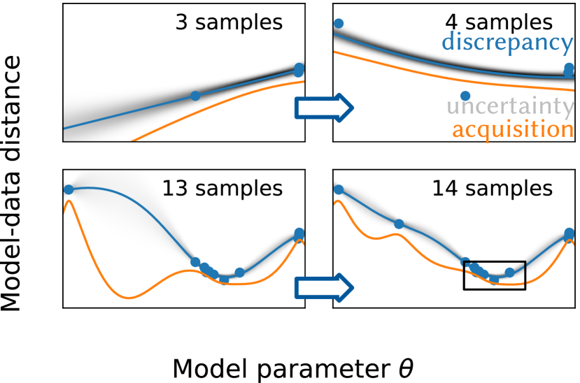 Abbildung 4: BOLFI sampling paradigm. A Gaussian Process approximates the relationship between the model-data distance and the model parameters, labelled as „discrepancy“ with „uncertainty“. An „acquisition“ function can be calculated from this Gaussian Process. The minimum of the „acquisition“ function gives the most informative next sample. Circles indicate the sample points. The black border in the bottom right plot indicates the cutout presented in Figure 5a.
Bayesian Optimization for Likelihood-Free Inference (BOLFI) was developed by Gutmann et al. 38. Applications of their algorithm include the fields of cosmology 55, ecology 56, genetics 57, and neurobiology 58. We use an implementation of BOLFI by Lintusaari et al. in the software ELFI 59. For further reading, we recommend the introduction to BOLFI in 60. To the best of our knowledge, we are the first to combine BOLFI with Expectation Propagation.
Bayesian Optimization takes the idea of preconditioning an estimation task with a Prior one step further: this class of algorithms utilizes each sample to optimize the choice of the following sample. This short-circuiting of the usual Bayesian recipe allows for the active selection of the most informative following sample, where standard Bayesian algorithms draw samples randomly. Figure 4 visualizes how BOLFI „explores“ the parameter search space before „exploiting“ the region where BOLFI expects the optimal parameter set. A sample is chosen by minimizing its „acquisition“ function in eq. 5. To this aim, a Gaussian Process is trained on the preceding simulation samples and acts as a fast surrogate for the intractable discrepancy-parameter relationship to enable this minimization.
BOLFI works best for low sample numbers. This is because it involves the inversion of a matrix with rank equal to the sample size at each sample. Expectation Propagation helps in this respect as it keeps the sample size small. Each feature update resets the samples to 0 and provides a more precise Prior for the next iteration. While this resolves the most significant weakness of BOLFI, it requires that the form of the current Posterior does not change over multiple site updates. Here, we limit ourselves to Gaussian distributions. The transformations can limit the parameters to positive numbers by taking the logarithm or to an interval by taking the tangent. Please note that any proper probability distribution can be optimized with BOLFI.
For each feature with index , the algorithm of BOLFI 38 starts with a user-defined number of (quasi-)random samples from the Prior. To achieve optimal integration efficiency, these samples stem from a Sobol sequence 61. These samples and the deviations between simulation and experiment constitute the data that BOLFI trains a surrogate function on. Here, is the current feature of the experimental data and is the simulated feature for the parameter set . For illustration, Figure 4 shows as blue dots over , where the blue line labelled „discrepancy“ would be that surrogate function.
The training points are assumed to follow a Gaussian Process with parabolic mean function. From this model, BOLFI applies a filter to this Gaussian Process to calculate the approximation to the model-simulation discrepancy ,
(4)
where is adjusted automatically. We show the derivation of this Posterior in the SI Section LABEL:SI-sec:BOLFI.
and constitute a differentiable surrogate function for the intractable model-simulation discrepancy function
Abbildung 4: BOLFI sampling paradigm. A Gaussian Process approximates the relationship between the model-data distance and the model parameters, labelled as „discrepancy“ with „uncertainty“. An „acquisition“ function can be calculated from this Gaussian Process. The minimum of the „acquisition“ function gives the most informative next sample. Circles indicate the sample points. The black border in the bottom right plot indicates the cutout presented in Figure 5a.
Bayesian Optimization for Likelihood-Free Inference (BOLFI) was developed by Gutmann et al. 38. Applications of their algorithm include the fields of cosmology 55, ecology 56, genetics 57, and neurobiology 58. We use an implementation of BOLFI by Lintusaari et al. in the software ELFI 59. For further reading, we recommend the introduction to BOLFI in 60. To the best of our knowledge, we are the first to combine BOLFI with Expectation Propagation.
Bayesian Optimization takes the idea of preconditioning an estimation task with a Prior one step further: this class of algorithms utilizes each sample to optimize the choice of the following sample. This short-circuiting of the usual Bayesian recipe allows for the active selection of the most informative following sample, where standard Bayesian algorithms draw samples randomly. Figure 4 visualizes how BOLFI „explores“ the parameter search space before „exploiting“ the region where BOLFI expects the optimal parameter set. A sample is chosen by minimizing its „acquisition“ function in eq. 5. To this aim, a Gaussian Process is trained on the preceding simulation samples and acts as a fast surrogate for the intractable discrepancy-parameter relationship to enable this minimization.
BOLFI works best for low sample numbers. This is because it involves the inversion of a matrix with rank equal to the sample size at each sample. Expectation Propagation helps in this respect as it keeps the sample size small. Each feature update resets the samples to 0 and provides a more precise Prior for the next iteration. While this resolves the most significant weakness of BOLFI, it requires that the form of the current Posterior does not change over multiple site updates. Here, we limit ourselves to Gaussian distributions. The transformations can limit the parameters to positive numbers by taking the logarithm or to an interval by taking the tangent. Please note that any proper probability distribution can be optimized with BOLFI.
For each feature with index , the algorithm of BOLFI 38 starts with a user-defined number of (quasi-)random samples from the Prior. To achieve optimal integration efficiency, these samples stem from a Sobol sequence 61. These samples and the deviations between simulation and experiment constitute the data that BOLFI trains a surrogate function on. Here, is the current feature of the experimental data and is the simulated feature for the parameter set . For illustration, Figure 4 shows as blue dots over , where the blue line labelled „discrepancy“ would be that surrogate function.
The training points are assumed to follow a Gaussian Process with parabolic mean function. From this model, BOLFI applies a filter to this Gaussian Process to calculate the approximation to the model-simulation discrepancy ,
(4)
where is adjusted automatically. We show the derivation of this Posterior in the SI Section LABEL:SI-sec:BOLFI.
and constitute a differentiable surrogate function for the intractable model-simulation discrepancy function
. Following the initial regression to the Sobol quasi-random samples, further samples are generated from the surrogate in eq. 4 in the following manner, called „lower confidence bound selection criterion“ 38. The next sample gets taken as the minimum value of the so-called acquisition function (5) where is a sufficiently large scaling factor that grows logarithmically with . 38 Figure 4 shows a visualization of the acquisition function, where is represented by the blue line and is the width of the grey-shaded region around that blue line, while the orange line represents the acquisition function itself. The minimum of the acquisition function approximates the parameter set with the highest chances of generating a simulation closest to the experiment. Hence, BOLFI generates samples sequentially and optimally to minimize the remaining uncertainty in the Likelihood estimation. After finishing the acquisition of samples, the final surrogate in eq. 4 forms the basis for the Likelihood approximation, as shown in Figure 5. In the Likelihood-Free Inference (LFI) framework, the approximation to the Likelihood is the probability that the discrepancy surrogate falls below a threshold value : (6) The threshold value is arbitrary in most LFI algorithms, but BOLFI infers it from the surrogate itself as . With the probability density function of the Gaussian surrogate, can be calculated as (7a) (7b) where is the cumulative distribution function of a standard normal variable, (8) Simultaneously regressing and sampling from the sampling distribution reduces the number of required samples by several orders of magnitude. 38
 Abbildung 5: Calculation of the Likelihood approximation in BOLFI. is defined in eq. 6. (a) Cutout of Figure 4 at 14 samples, zoomed in on the minimum of the discrepancy surrogate. The threshold is visualized as a green line. (b) The Likelihood is the integral of the discrepancy surrogate beneath the threshold.
Validation of EP-BOLFI performance
Tabelle 2: Performance comparison between MCMC 17 and EP-BOLFI. The estimation results refer to one standard deviation. true initial std. Aitio et al. (MCMC), EP-BOLFI EP-BOLFI EP-BOLFI parameter value deviation simulations sim. sim. sim. / / - / / / Our reference for state-of-the-art automated battery model parameterization is the work of Aitio et al. 17. They create two types of synthetic data with an SPMe model, multimodal sinusoidal excitations at eleven SOCs denoted „excitation-point case“ and a discharge with a superimposed small unimodal sinusoidal excitation denoted „wide-excursion case“. Aitio et al. fit five parameters with an MCMC algorithm: the electrolyte and solid diffusivities , , the cation transference number , and the variance of the white noise superimposed on the synthetic measurement. In the wide-excursion case, MCMC fits the parameters nicely. However, the MCMC algorithm finds a wide range of inconsistent values in the excitation-point case 17. We apply our EP-BOLFI algorithm to the same synthetic data with the same SPMe model as Aitio et al. 17. Aitio et al. take the -distance of the voltage as the cost function. For the EP-BOLFI algorithm, we preprocess the voltage response and define features. For the excitation-point cases, we perform a Fast Fourier Transform on the current input and voltage output to calculate the impedance for each mode as features. For the wide-excursion case, we use the -distances of four voltage curve segments as features. The results for the wide-excursion case are shown in Table 2. We observe that EP-BOLFI reaches a similar accuracy to that in Aitio et al. 17 with about 12 times less simulations, depending on the model parameter. Between and simulations for EP-BOLFI we observe an order of magnitude increase in accuracy, and at simulations all but are as accurately or even more accurateley estimated as by MCMC. The comparison of EP-BOLFI to MCMC in Aitio et al. 17 for the excitation-point case is shown in the SI Table LABEL:SI-tab:comparison. Across all excitation points, EP-BOLFI with simulations vastly outperforms the MCMC approach in terms of stability and accuracy. EP has the potential to deal with the data at all excitation points at once. Hence, we perform an additional experiment, collating the four excitation points 1, 2, 3 and 7 with the smallest uncertainties. While that leads to overfitting, the number of simulations required to reach convergence even shrinks to . This demonstrates that the computation time of EP scales favourably with the dimension of the data 37.Experimental
Experimental setup and a priori known parameters
Tabelle 3: The missing battery parameters and how we procure them. For the symbols, cf. Table 5. parameter source value A priori assumed parameters value for NMC-111 62 1.07 value for graphite 62 10.67 symmetry assumption 0.5 Subsection Measurement of the OCV curves GITT measurement 63 [0.0, 1.0] our GITT measurement [3.0, 5.0] scaling factor, cf. eq. 9 62 scaling factor, cf. eq. 9 62 scaling factor, cf. eq. 9 64 scaling factor, cf. eq. 9 64 Subsection Parameters fitted with EP-BOLFI EP-BOLFI fit TBD EP-BOLFI fit TBD EP-BOLFI fit TBD EP-BOLFI fit TBD EP-BOLFI fit TBD EP-BOLFI fit TBD EP-BOLFI fit TBD The full cell GITT data got measured at BASF. Here, we list the parameters known before starting our estimation algorithms, following the checklist in 65. The only points in that checklist we do not fulfill are „specifications of used materials“ and „coulombic efficiency“. The GITT measurement protocol consists of repeating sets of -, -, - and - pulses with occasional - pulses each 25% SOC (State-Of-Charge). corresponds to a theoretical capacity of . The rest periods at zero current between the pulses were , with the exception of the pulses, which were enclosed in rests. The GITT experiment was conducted at 25 °C. The minimum and maximum operating voltage of the cell are and , respectively. The GITT data spans from SOC 25% to 100%, i.e., 25% discharged to 100% discharged. The cell contains the following materials. The negative electrode mostly consists of graphite with 95.7% active material and is slightly overbalanced. The separator is Celgard 2500 with thickness. The positive electrode is 94% NCM-851005 with 3% Solef 5130, 2% SFG 6L and 1% Super C 65. The electrolyte is LiPF6 in EC:DEC 3:7 with 2% VS as SEI former. Here, we list the geometric parameters and the electrolyte properties. The cell is a square pouch cell. The cross-sectional areas are , , and for the negative electrode, separator, and positive electrode, respectively. The porosities are roughly 0.27, 0.55, and 0.29 for the negative electrode, separator, and positive electrode, respectively. The porosities of the electrodes were approximated by comparing their density with the bulk densities of graphite at and NCM-851005 at (times 94%), respectively. The porosity of the separator and its Bruggeman coefficient of 3.6 were taken from Patel et al. 66. The thicknesses of the electrodes are and for the negative and positive electrodes, respectively. Both thicknesses were calculated from densities and areal mass loadings, i.e. the mass of active material per cross-sectional area of the respective current collector. The areal mass loadings of the negative and positive electrode are and , respectively. Thus, the electrolyte volume is about and the volumetric ratio of electrolyte to active material is about 0.737. The electrolyte has cation transference number , thermodynamical factor , diffusivity , and conductivity . We take the a priori electrolyte parameters from Nyman et al. 67, even though they characterized EC:EMC 3:7, not EC:DEC 3:7. We neglect this disparity, since our focus is to demonstrate our parameterization procedure. We consider the cation transference number unknown with known error bounds and tie the thermodynamical factor to it as . At this point, we fixed most parameters. We discuss the remaining unknown parameters listed in Table 3 in the next subsections. We shortly discuss the few unknown parameters with negligible impact here. The electronic conductivities of the electrodes are from Danner et al. 62; there, the electrode materials were graphite and NMC-111. We accept the potential error due to the different materials, since the electronic conductivities typically only account for a static IR drop of up to at current . The charge-transfer coefficients, also known as asymmetry factors, are set to , i.e., we make the standard assumption that the charge-transfer reactions are symmetric.Measurement of the OCV curves
The Open-Cell Voltage (OCV) has by far the most significant effect on the overall operating cell voltage, typically about to . The minor voltage losses described by the equations in table 1 are due to the limiting transport processes and reactions the so-called „overpotential“. The overpotential is typically around . Hence, before we analyze cell processes via the overpotential, we need to know the OCV of the cell with high precision 68. The most precise measurement of the OCV is possible with GITT, with a voltage error of 63. Still, measurements at low constant current get often misused as „quasi-OCV“ (qOCV) measurements 30, 34. Chen et al. 31 demonstrate how constant-current curves exhibit significant deviations from OCV at high or low charge and between voltage plateaus, even at low current. Hence, we do not use qOCV measurements. We use the physics-inspired OCV model of Birkl et al. 63, as it assigns an SOC range to incomplete OCV data in an informed and automatic way. This SOC range will approximate the maximally lithiated and de-lithiated states of the positive electrode at SOCs 0 and 1, respectively. We denote that SOC range as „positive electrode SOC“ or . Likewise, we refer to the maximally lithiated and de-lithiated states of the negative electrode when we assign the „negative electrode SOC“ or . We fit the OCV curve of the positive electrode given the OCV curve of the negative electrode in Subsection Extracting positive electrode OCV from full-cell GITT. The maximum intercalation concentrations were fitted to the CC-CV and GITT data at the same time.Parameters fitted with EP-BOLFI
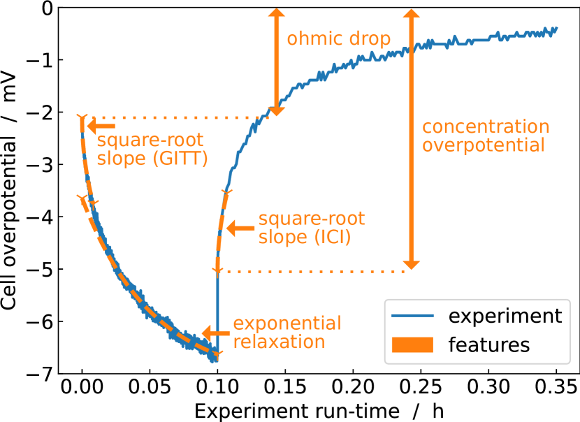 Abbildung 6: The five features for Expectation Propagation in the experimental data at each GITT pulse.
We now have seven model parameters of interest that we can fit to the GITT data, summarized in eq. 9. These are the model parameters that appear independently from unknown properties in our physics-based model,
(9)
For simplicity, we assume that these parameters are independent from electrolyte concentrations and location within the cell. We ignore the concentration dependence of the cation transference number 69. We assume that the Bruggeman coefficients are spatially constant. Spatially and concentration resolved measurements are required to parameterize these heterogeneities.
GITT measurements give us information about SOC dependence. The functional form of the exchange-current density
Abbildung 6: The five features for Expectation Propagation in the experimental data at each GITT pulse.
We now have seven model parameters of interest that we can fit to the GITT data, summarized in eq. 9. These are the model parameters that appear independently from unknown properties in our physics-based model,
(9)
For simplicity, we assume that these parameters are independent from electrolyte concentrations and location within the cell. We ignore the concentration dependence of the cation transference number 69. We assume that the Bruggeman coefficients are spatially constant. Spatially and concentration resolved measurements are required to parameterize these heterogeneities.
GITT measurements give us information about SOC dependence. The functional form of the exchange-current density
is an active topic of research 70, 71, 72, 73. Likewise, the active material diffusivities depend on electrode SOC 74. Hence, there are three parameters of interest that do not depend on SOC, namely , , and , and four that do depend on SOC, namely , , and . Therefore, we fit all seven parameters of interest in eq. 9 once to a pair of GITT pulses with different C-rates. Then, we hold the three SOC-independent parameters constant, and fit only the four SOC-dependent ones to all other GITT pulses. We also miss the geometric parameters for the electrode particles to correctly scale the active material diffusivities and the exchange-current densities . However, their absolute values can be corrected when the specific surface areas and particle radii get measured. Without loss of generality, we assume the specific surface area 64. Analogously, the particle radii are just a scaling factor in our model. We arbitrarily take the particle radii from a battery of Danner et al. 62. For Expectation Propagation, we reduce the experimental data to discrete features as visualized in Figure 6. The five features we fit are the voltage directly after the current has been shut off (concentration overpotential), the relaxation times during the discharge pulses, the ohmic voltage drop, and the GITT and ICI (Intermittent Current Interruption) square-root slopes 75 during discharge pulses and rest periods, respectively. We use the following fit function to obtain the square-root slopes and the offsets of the square-root segments : (10) where refers to the start of the current pulse or the start of the rest phase. The square-root function fitted to the current pulse gives the ohmic voltage drop as and the GITT square-root slope as . The square-root function fitted to the rest phase gives the concentration overpotential as and the ICI square-root slope as . To get the relaxation time , we use the following fit function on the current pulse: (11) where refers to the start of the current pulse. While our current pulses are too short to fulfill the requirements for ICI as an analytical formula, we will later see that our „incomplete“ ICI square root slopes still give valuable information. We omit the exponential relaxation at rest as a feature since it is difficult to fit uniquely 76, 69. This is discussed in Section Discussions. We omit and from the exponential fit function in eq. 11 as features, as they are less consistently fitted than the concentration overpotential, which contains much of the same information. The analysis of GITT and ICI with approximate formulas introduces some inaccuracy as discussed by Geng et al. 77. EP-BOLFI fits the whole DFN model directly to the experimentally observed square root slopes. A detailed discussion for the complementary relevance of both GITT and ICI features is performed in the SI Section LABEL:SI-sec:features. We emphasize that one might also use simple time segments of the data with their -distance as features for EP-BOLFI if no better preprocessing step is known. The features we chose have less interdependence than -segments, accelerating the computations and making the results more interpretable. As we can see in Figure 6, we capture the main information of the raw voltage curve in the five features. We choose normal distributions for the Bruggeman coefficient priors and the cation transference number, and log-normal distributions for the priors of all other parameters of interest. We motivate the log-normal distributions with the Arrhenius relation: reaction rates and diffusivities may be modelled as a reaction following an Arrhenius relation, and hence are log-normally distributed if the corresponding activation energies are normally distributed. In the spirit of Laplace approximations 78, a good approximation of the true distributions close to the true estimate is sufficient, even for global optimization. The bounds of the prior and posterior 95% confidence intervals and the most likely estimates are listed in Table 4.
Computational details
We employ the helpful checklist from Mistry et al. 79 to ensure that we include every aspect of sensitivity of numerical inputs. The filled-in checklist is in the SI Table LABEL:SI-tab:checklist in the SI Section LABEL:SI-sec:checklist. We discretize the 1D+1D model equations in table 1 with Spectral Volumes 80 and solve them with CasADi 81 interfaced through PyBaMM 82. Compared to Finite Volumes and the ode15s solver in MATLAB, our simulations run 20 times faster. The Spectral Volumes mesh is of order 8 in the electrolyte and the negative electrode particles and of order 20 in the positive electrode particles. For the electrolyte mesh, 2 Spectral Volumes are in the negative electrode, and 1 Spectral Volume each is in the separator and the positive electrode. We check for mesh independence by running a simulation with orders 16 and 40 instead of 8 and 20, respectively: the features change by no more than 0.2%. The timesteps are at most , and reducing them to at most changes the features by no more than 2%. Whenever we fit a parameterized function to data points, we use the trust-region algorithm for constrained optimization implemented in SciPy. The OCV model 63 we use gives the electrode SOC as a function of its OCV. Since the 1D+1D model equations in table 1 require the inverse function, we invert OCV model fits numerically and fit a spline to the inverse. Compared to direct spline fits to data, we retain the model-informed smoothing of the data and the estimation of the SOC range. Our algorithm can consider the uncertainties of all model parameters if the simulator function randomly samples them. Hence, we included the uncertainties of the SOC-independent fit parameters , and in the parameterization of the individual GITT pulses. For the initial fit of the SOC-dependent parameters, we choose the final GITT pulse in the dataset. The final GITT pulse corresponds to the most extreme SOC and, therefore, the largest overpotential, ideal for an initial fit. The SOC-dependent parameters and vary over two to four orders of magnitude, respectively. To allow for this parameter variability from one GITT pulse to the next, we magnify the error bars of the SOC-dependent parameters of one fit before we use them as Prior for the next fit. We limit the lower and upper bounds the priors could take to for the exchange-current densities and to [1e-14, 1e-10] for the electrode diffusivities. This limiter prevents the fit parameters from diverging into regions with infinite exchange-current density or instant diffusion. The error bars are then magnified to span at least half of the lower and upper bounds in the log scale. We fit the seven parameters of interest in eq. 9 to GITT data in Subsection Extracting model parameters with EP-BOLFI from GITT with our EP-BOLFI algorithm. We estimate parameters with warm-up samples and samples in total for BOLFI for each individual feature update, respectively. The pseudo-posteriors are estimated with an effective sample size of for , respectively, by the No-U-Turn-Sampler 83, a Markov-Chain Monte-Carlo sampler implemented in ELFI 59. We set up 4 EP iterations in both cases. We set the EP dampening parameter such that the total dampenings at the end are . For validation of our novel EP-BOLFI algorithm, we repeat the estimation procedures with one difference. We replace the measured data with synthetic simulated data for the most likely fit parameters. The better a given parameter is identifiable from the features, the closer the verification run would be to the first results. With this validation, we also make sure that EP-BOLFI converged, such that we can be sure that invisible non-identifiability issues arise purely from model and data. The total time for the estimation of seven parameters of interest with simulations on our office PC with an Intel Core i7-6700 at 4.00 GHz x 8 is about 20 hours. Of that, roughly twelve hours is the simulation time for simulations of two GITT pulses. The total time for the estimation of the four SOC-dependent parameters of interest with simulations for each pulse is about 120 minutes on our PC. Of that, roughly 80 minutes is the simulation time for simulations of one GITT pulse.Results from full-cell GITT data
Before we describe the application of EP-BOLFI to GITT data, we have to identify the OCV of the positive electrode in Subsection Extracting positive electrode OCV from full-cell GITT. The application of EP-BOLFI is then presented in Subsection Extracting model parameters with EP-BOLFI from GITT.Extracting positive electrode OCV from full-cell GITT
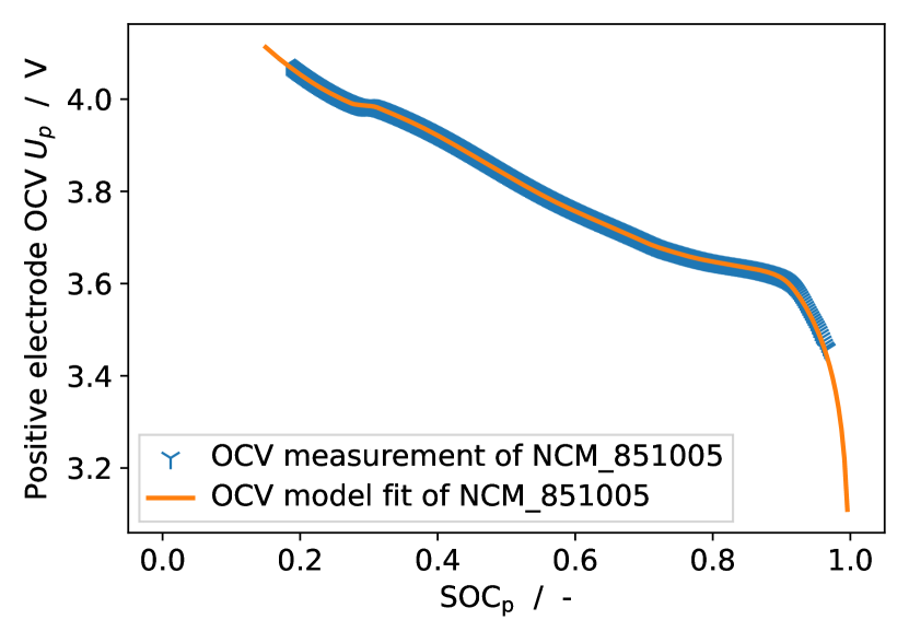 Abbildung 7: The model fit 63 of the OCV curve of the positive NCM-851005 electrode that we obtain by adding the OCV curve of the negative electrode to the GITT data. The root-mean-square-error is and the mean absolute error is .
We want to obtain the open-circuit voltage (OCV) of the positive electrode. Since we do not have half-cell data, our estimation relies on our approximate knowledge of the OCV of the negative electrode 63.
As a first step, we determine the cell balancing, i.e., the negative electrode SOC as a function of the positive electrode SOC. To find the cell balancing, we determine an approximate second derivative of from the data. We obtain that by shifting the CC curves by the CV step against each other, adding them, and subtracting the GITT curve two times. The derivation of this preprocessing step and the utilized data are laid out in the SI Section LABEL:SI-sec:OCV_preprocessing.
We compare the second derivative of to that of a known graphite OCV curve 63 in the SI Section LABEL:SI-sec:OCV_preprocessing. Though being a rough approximation, we can identify the peak positions of the second derivative. We find that the negative electrode SOC ranges from 3% to 84% over the SOC range of the positive electrode.
Taking into account this cell balance, we obtain from the sum of and the cell OCV from GITT data in Figure 7. We find that the cell capacity is . The OCV model of Birkl et al. 63 with eight phases gets fitted to the SOC range and we trust its extrapolation to the SOC range . We ignore OCV hysteresis effects 63 and only consider the discharge direction from now on.
Abbildung 7: The model fit 63 of the OCV curve of the positive NCM-851005 electrode that we obtain by adding the OCV curve of the negative electrode to the GITT data. The root-mean-square-error is and the mean absolute error is .
We want to obtain the open-circuit voltage (OCV) of the positive electrode. Since we do not have half-cell data, our estimation relies on our approximate knowledge of the OCV of the negative electrode 63.
As a first step, we determine the cell balancing, i.e., the negative electrode SOC as a function of the positive electrode SOC. To find the cell balancing, we determine an approximate second derivative of from the data. We obtain that by shifting the CC curves by the CV step against each other, adding them, and subtracting the GITT curve two times. The derivation of this preprocessing step and the utilized data are laid out in the SI Section LABEL:SI-sec:OCV_preprocessing.
We compare the second derivative of to that of a known graphite OCV curve 63 in the SI Section LABEL:SI-sec:OCV_preprocessing. Though being a rough approximation, we can identify the peak positions of the second derivative. We find that the negative electrode SOC ranges from 3% to 84% over the SOC range of the positive electrode.
Taking into account this cell balance, we obtain from the sum of and the cell OCV from GITT data in Figure 7. We find that the cell capacity is . The OCV model of Birkl et al. 63 with eight phases gets fitted to the SOC range and we trust its extrapolation to the SOC range . We ignore OCV hysteresis effects 63 and only consider the discharge direction from now on.
Extracting model parameters with EP-BOLFI from GITT
Tabelle 4: The prior 95% bounds and posterior standard deviation bounds for the 7-parameter estimation, including the most likely estimate. Parameter prior bounds posterior estimate [1.0, 100.0] 12.3, [10.2, 14.8] [1.0, 100.0] 36.3, [29.9, 44.0] [1e-14, 1e-10] (1.19, [0.82, 1.73])e-11 [1e-14, 1e-10] (0.82, [0.56, 1.22])e-11 [0.2, 0.4] 0.349, [0.343, 0.355] [1.8, 4.2] 2.72, [2.64, 2.81] [1.8, 4.2] 3.06, [2.99, 3.13]
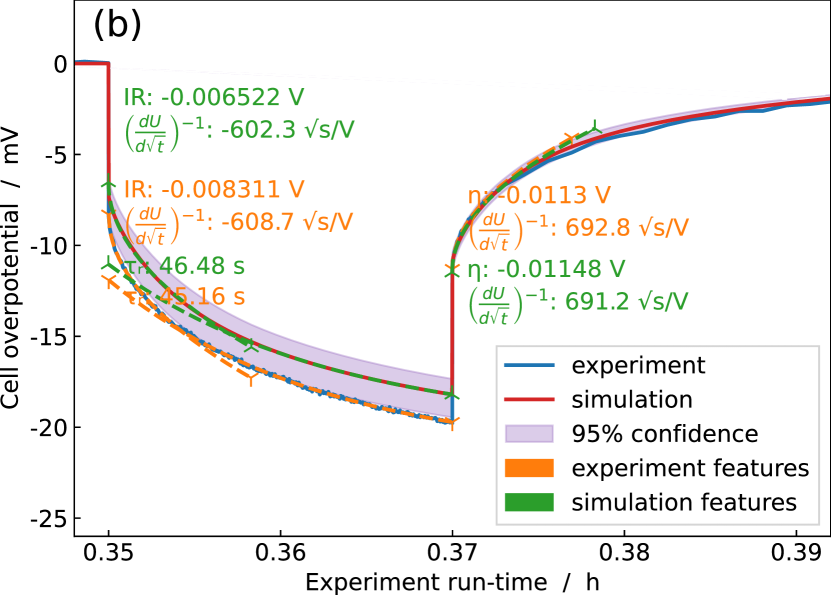
 Abbildung 9: The correlation matrix of the estimation result for 7 model parameters from two GITT pulses.
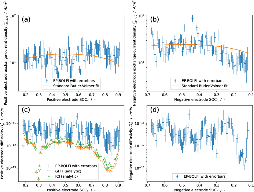 Abbildung 10: (a) , (b) , (c) and (d) estimates with error bars corresponding to one standard deviation of the logarithmic parameters. The comparison to a standard Butler-Volmer fit (see eq. 1h) shows that we can not use the results for and . However, if other parameters have been fitted correctly, their uncertainty then considers that and are effectively unknown. The results for are similar to those with half-cell GITT data from Schmalstieg et al. 84, Figure 7, apart from the wrong scaling. For , we plot the results of the analytic formulas for GITT and ICI for comparison. For and we plot the corresponding OCV curves of their respective electrode.
 Abbildung 11: Summary plots where the circles indicate the mean and the bars indicate plus-minus one standard deviation. (a) The relative comparison of the verification run with the original fit parameters in log-space. We fit the DFN model to itself for each GITT pulse estimation to see if it identifies the same parameters. (b) The relative deviation of the fitted simulated features to the experimental features. We see that all features but the exponential relaxation time get close to the 2% accuracy with which we simulate the features.
With the procedure laid out in Subsection Computational details, we fit seven parameters to GITT pulses 66 () and 67 () in the data. We choose these pulses since the OCV curves of both electrodes have significant gradients there, which improves the sensitivity of our experimental data to electrode diffusivities 75. Our prior bounds are based on the LiionDB database 85 and an order-of-magnitude estimate of the exchange-current densities and active material diffusivities. We show the fitting results as estimates and 95% confidence intervals in Table 4.
In Figure 8, we depict the five fit features in the experiment and how we predict them in the simulation. The good agreement between features in simulation and data at low and high current verifies our optimization. The square-root GITT and ICI features have an excellent agreement. However, there is a significant difference in fit quality between low () and high () current for the exponential relaxation. We discuss that electrode heterogeneity can explain this mismatch (see Section Discussions). We find direct relationships between features and parameters below; thus, the excellent fit of most of the features gives insights on its own. Figure 8a is a good example to illustrate our featurization approach. If we had optimized the model for the time series, the simulation would cut across the voltage measurements, matching neither short-term nor long-term processes in the battery.
We now discuss the correlation matrix, i.e., the covariance matrix normalized by the variances. In Figure 9, the correlation matrix indicates how a parameter change affects the estimates of the other parameters. Each matrix entry shows how the (lack of) knowledge of some parameters influences the accuracy of the other parameters. Correlations close to 0 indicate that the two parameters are not coupled in the data as interpreted by our model. Note that the two exchange-current densities are correlated with each other in our full cell examination. We see correlations between the SOC-independent model parameters and the SOC-dependent ones, especially between the diffusivity of the positive electrode and both Bruggeman coefficients. We rerun the estimation procedure twice with different initial random seeds to validate that these correlations are consistent properties of model and data rather than numerical artefacts. The corresponding data are in the accompanying GitHub repository. These correlations demonstrate the benefit of estimating all seven parameters together, namely that we obtain a consistent parameter set.
Next, we fit all GITT pulses with only the SOC-dependent four parameters , , and under consideration of the remaining uncertainty of , and . In Figure 10, we plot the optimal estimates and error bars corresponding to one standard deviation of the logarithmic parameters as a function of electrode SOC. Please note that we define „electrode SOC“ by the theoretical minimum and maximum lithiation of an electrode. The error bars in Figure 10 show us how precise the parameters are estimated in each GITT pulse.
We compare the exchange-current densities in Figure 10a and Figure 10b with the standard SOC-dependence of the Butler-Volmer rate in eq. 1h 71. One reason for the large error bars is that the two exchange-current densities primarily act as interchangeable resistances. In the SI Figure LABEL:SI-fig:joint_resistance, we plot their joint resistance. Since it is not much smoother and has large error bars, we can conclude that there are more identifiability issues than just the interchangeability of the two exchange-current densities. The low identifiability is not surprising, as GITT was not designed with measuring exchange-current densities in mind. Both exchange-current densities are visible in measurements on much smaller timescales 6 than the GITT pulses used here, which means that they mostly collectively show up as a contribution to the ohmic drop.
The diffusivities in Figure 10c and Figure 10d are smoother functions of SOC. The error bars are still more prominent than in a half-cell setup, for which GITT was initially designed 5. We attribute the larger error bars to a limited discernability of the two electrodes in the data. To discuss the results for , we plot the results of the analytic formulas for the GITT and ICI methods 75 for in Figure 10c. We show these formulas in the SI Eq. 8.37. These formulas neglect the influence of the negative electrode and the electrolyte; hence, there is no equivalent formula for . We instead compare with a measurement by Schmalstieg et al. 84.
The results for in Figure 10c have fairly small error bars and seem to be rather constant, in contrast to the analytical GITT and ICI formulas. The analytical formulas have especially large deviations from our results in the regions around and . At the positive electrode OCV curve has a very flat plateau that impedes the analytic formula and introduces large uncertainty to it. At the low diffusivity of the negative electrode at corresponding may disturb the analytical formulas. EP-BOLFI, instead, produces consistent estimates for both diffusivities and can even distinguish between the two electrodes. Hence, the prediction of the uncertainty displayed in Figure 10c gives us further information about the completeness of the experimental data and the predictability of the model parameters.
The results for in Figure 10d exhibit slightly smaller error bars than those for and reproduce the literature data of Schmalstieg et al. 84 well. They observe the same shape of the diffusivity curve in a half-cell with graphite, especially the dip around . Kang et al. 86 perform a detailed analysis of the possible sources of uncertainty, such as the duration or intensity of the current pulses.
Please note that we can not determine the absolute magnitude of the estimates for and , as they depend on the unknown particle radius and , respectively. We emphasize that we can identify and separately, as indicated by their weak correlation in Figure 9 and their agreement with expected behaviours. We achieve this even though we measured a full cell and do not know the electrolyte properties perfectly.
In Figure 11a we verify how reliable our parameterization result is. For this purpose, we create synthetic data from a DFN model with the parameters we fitted to the experimental data (see Figure 8). We apply EP-BOLFI to this SOC-dependent synthetic data in a verification run. We depict here the relative deviation between the true and estimated parameters in this verification run. As the fitted probability distributions are log-normal, we observe the relative deviations on a log-scale. We confirm that the solid diffusivities are identifiable within 1% accuracy. Notably, the exchange-current densities show a much larger variability in accuracy, matching their erratic behaviour in 10ab. We conclude that the diffusivities in Figure 10cd can be trusted at most SOC, while the exchange currents in Figure 10ab are not clearly identifiable from GITT. We also verify that the model justifies the limitation to a Gaussian Posterior with only one mode since multiple distant sets of equally optimal parameters would result in far poorer accuracy.
In Figure 11b, we verify that the parameterization accurately reproduced the experimental data. For that, we collect the deviations between features in the experimental data to the features in the fitted simulated data. We see that all features were fitted well except for the exponential relaxation time . We conclude that is an unreliable feature in our GITT dataset with the DFN model.
In the SI Section LABEL:SI-sec:sensitivity, we perform a complementary sensitivity analysis on the DFN model at the fitted parameters at each GITT pulse. Based on these sensitivities, we can identify parameters that appear to be fitted well in Figure 11a, but depend on unreliable features in Figure 11b. As we can see in the SI Figure LABEL:SI-fig:sensitivities, and both depend on all features but the ohmic resistance, with being more sensitive to the concentration overpotential than . We find that all four SOC-dependent parameters also have a consistently high sensitivity to the exponential relaxation time , which we just ruled out as a reliable feature. Despite that sensitivity, EP-BOLFI automatically ignored in favour of fitting the parameters more consistently with other features. We conclude that we can nicely estimate and accurately from our GITT dataset because they are sensitive to the square-root features and the concentration overpotential.
Abbildung 11: Summary plots where the circles indicate the mean and the bars indicate plus-minus one standard deviation. (a) The relative comparison of the verification run with the original fit parameters in log-space. We fit the DFN model to itself for each GITT pulse estimation to see if it identifies the same parameters. (b) The relative deviation of the fitted simulated features to the experimental features. We see that all features but the exponential relaxation time get close to the 2% accuracy with which we simulate the features.
With the procedure laid out in Subsection Computational details, we fit seven parameters to GITT pulses 66 () and 67 () in the data. We choose these pulses since the OCV curves of both electrodes have significant gradients there, which improves the sensitivity of our experimental data to electrode diffusivities 75. Our prior bounds are based on the LiionDB database 85 and an order-of-magnitude estimate of the exchange-current densities and active material diffusivities. We show the fitting results as estimates and 95% confidence intervals in Table 4.
In Figure 8, we depict the five fit features in the experiment and how we predict them in the simulation. The good agreement between features in simulation and data at low and high current verifies our optimization. The square-root GITT and ICI features have an excellent agreement. However, there is a significant difference in fit quality between low () and high () current for the exponential relaxation. We discuss that electrode heterogeneity can explain this mismatch (see Section Discussions). We find direct relationships between features and parameters below; thus, the excellent fit of most of the features gives insights on its own. Figure 8a is a good example to illustrate our featurization approach. If we had optimized the model for the time series, the simulation would cut across the voltage measurements, matching neither short-term nor long-term processes in the battery.
We now discuss the correlation matrix, i.e., the covariance matrix normalized by the variances. In Figure 9, the correlation matrix indicates how a parameter change affects the estimates of the other parameters. Each matrix entry shows how the (lack of) knowledge of some parameters influences the accuracy of the other parameters. Correlations close to 0 indicate that the two parameters are not coupled in the data as interpreted by our model. Note that the two exchange-current densities are correlated with each other in our full cell examination. We see correlations between the SOC-independent model parameters and the SOC-dependent ones, especially between the diffusivity of the positive electrode and both Bruggeman coefficients. We rerun the estimation procedure twice with different initial random seeds to validate that these correlations are consistent properties of model and data rather than numerical artefacts. The corresponding data are in the accompanying GitHub repository. These correlations demonstrate the benefit of estimating all seven parameters together, namely that we obtain a consistent parameter set.
Next, we fit all GITT pulses with only the SOC-dependent four parameters , , and under consideration of the remaining uncertainty of , and . In Figure 10, we plot the optimal estimates and error bars corresponding to one standard deviation of the logarithmic parameters as a function of electrode SOC. Please note that we define „electrode SOC“ by the theoretical minimum and maximum lithiation of an electrode. The error bars in Figure 10 show us how precise the parameters are estimated in each GITT pulse.
We compare the exchange-current densities in Figure 10a and Figure 10b with the standard SOC-dependence of the Butler-Volmer rate in eq. 1h 71. One reason for the large error bars is that the two exchange-current densities primarily act as interchangeable resistances. In the SI Figure LABEL:SI-fig:joint_resistance, we plot their joint resistance. Since it is not much smoother and has large error bars, we can conclude that there are more identifiability issues than just the interchangeability of the two exchange-current densities. The low identifiability is not surprising, as GITT was not designed with measuring exchange-current densities in mind. Both exchange-current densities are visible in measurements on much smaller timescales 6 than the GITT pulses used here, which means that they mostly collectively show up as a contribution to the ohmic drop.
The diffusivities in Figure 10c and Figure 10d are smoother functions of SOC. The error bars are still more prominent than in a half-cell setup, for which GITT was initially designed 5. We attribute the larger error bars to a limited discernability of the two electrodes in the data. To discuss the results for , we plot the results of the analytic formulas for the GITT and ICI methods 75 for in Figure 10c. We show these formulas in the SI Eq. 8.37. These formulas neglect the influence of the negative electrode and the electrolyte; hence, there is no equivalent formula for . We instead compare with a measurement by Schmalstieg et al. 84.
The results for in Figure 10c have fairly small error bars and seem to be rather constant, in contrast to the analytical GITT and ICI formulas. The analytical formulas have especially large deviations from our results in the regions around and . At the positive electrode OCV curve has a very flat plateau that impedes the analytic formula and introduces large uncertainty to it. At the low diffusivity of the negative electrode at corresponding may disturb the analytical formulas. EP-BOLFI, instead, produces consistent estimates for both diffusivities and can even distinguish between the two electrodes. Hence, the prediction of the uncertainty displayed in Figure 10c gives us further information about the completeness of the experimental data and the predictability of the model parameters.
The results for in Figure 10d exhibit slightly smaller error bars than those for and reproduce the literature data of Schmalstieg et al. 84 well. They observe the same shape of the diffusivity curve in a half-cell with graphite, especially the dip around . Kang et al. 86 perform a detailed analysis of the possible sources of uncertainty, such as the duration or intensity of the current pulses.
Please note that we can not determine the absolute magnitude of the estimates for and , as they depend on the unknown particle radius and , respectively. We emphasize that we can identify and separately, as indicated by their weak correlation in Figure 9 and their agreement with expected behaviours. We achieve this even though we measured a full cell and do not know the electrolyte properties perfectly.
In Figure 11a we verify how reliable our parameterization result is. For this purpose, we create synthetic data from a DFN model with the parameters we fitted to the experimental data (see Figure 8). We apply EP-BOLFI to this SOC-dependent synthetic data in a verification run. We depict here the relative deviation between the true and estimated parameters in this verification run. As the fitted probability distributions are log-normal, we observe the relative deviations on a log-scale. We confirm that the solid diffusivities are identifiable within 1% accuracy. Notably, the exchange-current densities show a much larger variability in accuracy, matching their erratic behaviour in 10ab. We conclude that the diffusivities in Figure 10cd can be trusted at most SOC, while the exchange currents in Figure 10ab are not clearly identifiable from GITT. We also verify that the model justifies the limitation to a Gaussian Posterior with only one mode since multiple distant sets of equally optimal parameters would result in far poorer accuracy.
In Figure 11b, we verify that the parameterization accurately reproduced the experimental data. For that, we collect the deviations between features in the experimental data to the features in the fitted simulated data. We see that all features were fitted well except for the exponential relaxation time . We conclude that is an unreliable feature in our GITT dataset with the DFN model.
In the SI Section LABEL:SI-sec:sensitivity, we perform a complementary sensitivity analysis on the DFN model at the fitted parameters at each GITT pulse. Based on these sensitivities, we can identify parameters that appear to be fitted well in Figure 11a, but depend on unreliable features in Figure 11b. As we can see in the SI Figure LABEL:SI-fig:sensitivities, and both depend on all features but the ohmic resistance, with being more sensitive to the concentration overpotential than . We find that all four SOC-dependent parameters also have a consistently high sensitivity to the exponential relaxation time , which we just ruled out as a reliable feature. Despite that sensitivity, EP-BOLFI automatically ignored in favour of fitting the parameters more consistently with other features. We conclude that we can nicely estimate and accurately from our GITT dataset because they are sensitive to the square-root features and the concentration overpotential.
Discussions
We gain three benefits from our Bayesian method, EP-BOLFI. The first benefit is universality; treating the model as a black box allows us to change the equations and fit parameters arbitrarily. The second benefit is global optimization, i.e., the thorough exploration of the range of feasible parameters. The third benefit is that we consistently estimate both the fit parameters and their uncertainty with only one algorithm. State-of-the-art battery parameterization most often requires a complicated calculation of the parameter-output-gradient 18, 24. For example, Sethurajan et al. 18 and Zhao et al. 24 conduct microscopic imaging of electrolyte concentration profiles. They then apply gradient-based iterative optimization to diffusion equations to extract electrolyte properties. While this specialization produces fantastic results, adapting their algorithm to other battery parameters or differential equations would warrant a new paper. With our algorithm, you only need to update the simulator and the feature definitions. The „exploration“ aspect of BOLFI ensures that it evenly minimizes the remaining uncertainty across the whole parameter search space. A gradient-based approach would be limited to the estimate „closest“ to the initial guess. Repeating the gradient-based optimization from various starting points can alleviate this locality problem, but it quickly becomes infeasible with a growing number of estimated parameters. The Bayesian analysis of Sethurajan et al. 18 and Zhao et al. 24 is preceded by a gradient-based optimization. EP-BOLFI is stable enough not to require this step, drastically cutting down on the implementation effort while incorporating a more expansive parameter space into the uncertainty estimate. The comparable computation time for the simulations and the EP-BOLFI algorithm shows a considerable cost to optimizing the samples. Compared to Aitio et al. 17, we require at least 12 times fewer samples for the estimation of five parameters. Hence, we significantly reduce the computation time and enable the simultaneous estimation of more than four parameters. The primary use of our technique is model parameterization, i.e., it tunes the model for predictive simulations, e.g., for a digital twin. Depending on the sophistication of the model, its parameters might be very close to the actual material properties. Thus, we may also characterize the battery non-destructively multiple times over its lifetime. Established characterization techniques usually require separate setups with Li-metal electrodes or destructive disassembly 5, 8, 31. Our results for are comparable to those of a half-cell GITT measurement 84, indicating that we extract the actual electrode property rather than some effective cell parameter. We believe that directly fitting continuum models includes significant coupled effects that analytic approximations can not describe. For example, the analytical formulas for GITT date back to 1977 5, and are only accurate for electrodes whose Open-Circuit Voltage (OCV) is locally describable by a Nernst equation. Modern electrode materials feature OCV curves with plateaus and kinks that severely impact GITT measurements, as we saw in Subsection Extracting model parameters with EP-BOLFI from GITT in Figure 10c. Our approach is less sensitive to this problem, as seen in Figure 10c. Our focus is salvaging CC-CV and GITT measurements and other organically grown measurement protocols such as WLTP since they constitute most of the experimental data available. Hence, our algorithm can also deal with raw data that is simply divided into multiple time segments, where their respective -distances between measurement and data would be the features. Such a segmentation reproduces the total -distance while utilizing the benefits of Expectation Propagation. The result is a better global -fit with less computational cost. This flexibility alleviates the dependence on data that is generated specifically for optimal parameter estimation performance 87. We can optimize a fitting procedure itself using the results of our algorithm. By studying the itemized correlation matrices for each feature, we can select the feature set with the clearest distinguishability between fit parameters. An analysis of the individual identifiability of each fit parameter is possible with either the diagonal of the covariance matrix or an interval analysis with the corresponding 95% confidence intervals. The poor agreement between model and data exponential relaxation times at rest is likely due to the artificial homogeneity of the DFN model. The spatial heterogeneities of a battery cell significantly impact its performance and are best captured by microstructure-resolved modelling 88, 12. The link between exponential relaxation times at rest and heterogeneity has been discussed by Kirk et al. 89. They propose at least a multi-particle 1D+1D model, the MP-DFN, that incorporates the different length scales of the electrode particles.Conclusion
Our newly developed algorithm EP-BOLFI is an optimizer that only requires the to-be-optimized model while minimizing the algorithm setup and the model evaluations. At the same time, the results of EP-BOLFI grant further insight into the data and the measurement uncertainty. EP-BOLFI and the data we applied it to are freely available. The GitHub repository containing the algorithm and the data is linked in Section Code availability. We show that EP-BOLFI is more robust than MCMC, while simultaneously being an order of magnitude faster. The segmentation into expert-informed features allows the algorithm to reliably match the model to the parts of the data that it can actually reproduce. We successfully parameterize a DFN model to a real full-cell GITT experiment while treating the model as a black box. „Black box“ refers to the fact that EP-BOLFI does not require a pre-calculated gradient of the model-data discrepancy with the model parameters. Our results extract both electrode diffusivities, which would not be possible with the analytical GITT formula. The non-destructive parameterization of models for the SEI 90, double-layers 91, and plating 4 might be possible with our algorithm. We expect to elucidate important correlations between these effects. EP-BOLFI allows to combine different measurement techniques for parameterisation. For example, Electrochemical Impedance Spectroscopy (EIS) can distinguish processes occurring at different time scales like reaction kinetics. This is a deficiency of GITT, as shown in this article. EP-BOLFI could fit EIS and GITT measurements simultaneously and determine a greater parameter set. An adaptation of our algorithm to faster simulators or more parallel processing power may swap out BOLFI for Robust Optimization Monte Carlo (ROMC) 92, implemented in ELFI 59. For fitting a large number of features, EP may be (partially) parallelized. The EP features can be updated iteratively or in parallel. But they can alternatively be updated in a in-between manner, where one can still reap some of the benefits of iterative preconditioning while utilizing more parallel processing power 37.Code availability
The bytecode of the presented EP-BOLFI optimization algorithm and the code which we use to create the figures is available at the following GitHub repository:https://github.com/YannickNoelStephanKuhn/EP-BOLFI.
The source code of EP-BOLFI will be available at that same GitHub repository at a later date. The experimental data is there as well in the „Releases“ section. Tabelle 5: Physical battery parameters and their non-dimensionalizations. s: active material phase. e: electrolyte. se: electrolyte-electrode interface. n/p: negative/positive electrode. s: separator. ∗: dimensional symbol. or : arbitrary reference parameter. Parameters Units Description Non-dimensionalization Spatial and temporal discretization Thickness of the cell Thickness of cell component Spatial coordinate through the cell Radius of electrode particles Radial coordinate through a particle Discharge timescale Time since beginning of experiment Electrolyte variables Electrolyte concentration Electrolyte potential Electrolyte ionic current density Molar ionic flux Electrode variables Concentration of intercalated lithium Electrode potential Electrolyte-Electrode interface reaction variables Electrode electronic current density Reaction overpotential Intercalation reaction current density Operating conditions Current density applied to the battery Temperature of the cell Electrolyte parameters Electrolyte diffusivity Electrolyte ionic conductivity – Cation transference number – – Thermodynamic factor – Electrode parameters – Electrode porosity – – Electrode Bruggeman coefficient – Electrode active material diffusivity Electrode electronic conductivity Electrode surface area to volume ratio Open-Cell Voltage (OCV) Electrolyte-Electrode interface reaction variables – Reaction symmetry factors – – Charge transfer numbers – Exchange-current density Tabelle 6: Scalings used for non-dimensionalization. Symbol Units Description Definition Discharge timescale Electrolyte transport timescale – Ratio of electrolyte transport and discharge timescales – Ratio of electrolyte and electrode concentration – Ratio of thermal voltage to ionic resistance Particle transport timescale – Ratio of partical transport and discharge timescales – Maximum electrode through maximum positive electrode concentration Intercalation reaction timescale – Ratio of reaction to discharge timescale
Acknowledgements
This work was supported by the German Aerospace Center (DLR). The authors thank BASF for providing the experimental data. The authors acknowledge support by the Helmholtz Association through grant no KW-BASF-6 (Initiative and Networking Fund as part of the funding measure „ZeDaBase-Batteriezelldatenbank“). This work contributes to the research performed at CELEST (Center for Electrochemical Energy Storage Ulm-Karlsruhe).Conflict of Interest
The authors declare no conflict of interest.ORCID
Yannick KuhnBirger Horstmann
Arnulf Latz
Keywords:
Literatur
- [1] A. Latz, J. Zausch, J. Power Sources 2011, 196, 3296.
- [2] K. D. Fong, J. Self, B. D. McCloskey, K. A. Persson, Macromol. 2021, 54, 2575.
- [3] F. Single, B. Horstmann, A. Latz, Phys. Chem. Chem. Phys. 2016, 18, 17810.
- [4] S. Hein, T. Danner, A. Latz, ACS Appl. Energy Mater. 2020, 3, 8519.
- [5] W. Weppner, R. A. Huggins, J. Electrochem. Soc. 1977, 124, 1569.
- [6] C. Heubner, M. Schneider, A. Michaelis, J. Electroanal. Chem. 2016, 767, 18.
- [7] N. Meddings, M. Heinrich, F. Overney, J. S. Lee, V. Ruiz, E. Napolitano, S. Seitz, G. Hinds, R. Raccichini, M. Gaberšček, J. Park, J. Power Sources 2020, 480, 228742.
- [8] A. K. Sethurajan, S. A. Krachkovskiy, I. C. Halalay, G. R. Goward, B. Protas, J. Phys. Chem. B 2015, 119, 12238.
- [9] M. Gouverneur, J. Kopp, L. V. Wüllen, M. Schönhoff, Phys. Chem. Chem. Phys. 2015, 17, 30680.
- [10] J. S. Horner, G. Whang, D. S. Ashby, I. V. Kolesnichenko, T. N. Lambert, B. S. Dunn, A. A. Talin, S. A. Roberts, ACS Appl. Energy Mater. 2021, 4, 11460.
- [11] A. M. Bizeray, J. H. Kim, S. R. Duncan, D. A. Howey, IEEE Trans. Control Syst. Technol. 2019, 27, 1862.
- [12] L. J. Bolay, T. Schmitt, S. Hein, O. S. Mendoza-Hernandez, E. Hosono, D. Asakura, K. Kinoshita, H. Matsuda, M. Umeda, Y. Sone, A. Latz, B. Horstmann, J. Power Sources Adv. 2022, 14, 100083.
- [13] J. C. Forman, S. J. Moura, J. L. Stein, H. K. Fathy, J. Power Sources 2012, 210, 263.
- [14] W. Li, I. Demir, D. Cao, D. Jöst, F. Ringbeck, M. Junker, D. U. Sauer, Energy Storage Mater. 2022, 44, 557.
- [15] G. L. Plett, J. Power Sources 2006, 161, 1369.
- [16] G. L. Plett, J. Power Sources 2004, 134, 277.
- [17] A. Aitio, S. G. Marquis, P. Ascencio, D. Howey, IFAC-PapersOnLine 2020, 53, 12497.
- [18] A. Sethurajan, S. Krachkovskiy, G. Goward, B. Protas, J. Comput. Chem. 2019, 40, 740.
- [19] L. Xu, X. Lin, Y. Xie, X. Hu, Energy Storage Mater. 2022, 45, 952.
- [20] T. Yamanaka, Y. Takagishi, T. Yamaue, J. Electrochem. Soc. 2020, 167, 100516.
- [21] A. Bills, S. Sripad, W. L. Fredericks, M. Guttenberg, D. Charles, E. Frank, V. Viswanathan, ChemRxiv 2020.
- [22] G. Houchins, V. Viswanathan, J. Chem. Phys. 2020, 153.
- [23] W. Li, J. Zhang, F. Ringbeck, D. Jöst, L. Zhang, Z. Wei, D. U. Sauer, J. Power Sources 2021, 506, 230034.
- [24] H. Zhao, R. D. Braatz, M. Z. Bazant, J. Comput. Phys. 2021, 436.
- [25] M. C. Krygier, T. LaBonte, C. Martinez, C. Norris, K. Sharma, L. N. Collins, P. P. Mukherjee, S. A. Roberts, Nat. Commun. 2021, 12, 1.
- [26] F. Biebl, T. Cvjetkovic, J. oliver Schwarz, E. Glatt, A. Grießer, C. Wagner, A. Wiegmann, Conf. Ind. Comput. Tomogr. 2019, pages 1–4.
- [27] O. Furat, D. P. Finegan, D. Diercks, F. Usseglio-Viretta, K. Smith, V. Schmidt, J. Power Sources 2021, 483, 229148.
- [28] J. Scharf, M. Chouchane, D. P. Finegan, B. Lu, C. Redquest, M. cheol Kim, W. Yao, A. A. Franco, D. Gostovic, Z. Liu, M. Riccio, F. Zelenka, J.-M. Doux, Y. S. Meng, Nat. Nanotechnol. 2022, 17, 446.
- [29] C. R. Birkl, M. R. Roberts, E. McTurk, P. G. Bruce, D. A. Howey, J. Power Sources 2017, 341, 373.
- [30] S. Tang, Z. Wang, H. Guo, J. Wang, X. Li, G. Yan, Solid State Ionics 2019, 343, 115083.
- [31] C.-H. Chen, F. B. Planella, K. O’Regan, D. Gastol, W. D. Widanage, E. Kendrick, J. Electrochem. Soc. 2020, 167, 080534.
- [32] A. Maheshwari, M. A. Dumitrescu, M. Destro, M. Santarelli, J. Power Sources 2016, 307, 160.
- [33] J. M. Escalante, S. Sahu, J. M. Foster, B. Protas, Electrochem. Soc. 2021, 168, 110519.
- [34] S. Park, D. Kato, Z. Gima, R. Klein, S. Moura, J. Electrochem. Soc. 2018, 165, A1309.
- [35] J. Zhao, M. Cano, J. J. Giner-Casares, R. Luque, G. Xu, Energy Environ. Sci. 2020, 13, 2618.
- [36] P. Gasper, K. Gering, E. Dufek, K. Smith, J. Electrochem. Soc. 2021, 168, 020502.
- [37] S. Barthelmé, N. Chopin, V. Cottet, Handbook of Approximate Bayesian Computation, Chapman and Hall/CRC, 1st editio edition 2018.
- [38] M. U. Gutmann, J. Corander, J. Mach. Learn. Res. 2016, 17, 1.
- [39] T. Schmitt, A. Latz, B. Horstmann, Electrochim. Acta 2020, 333, 135491.
- [40] S. G. Marquis, V. Sulzer, R. Timms, C. P. Please, S. J. Chapman, J. Electrochem. Soc. 2019, 166, A3693.
- [41] M. Doyle, T. F. Fuller, J. Newman, J. Electrochem. Soc. 1993, 140, 1526.
- [42] M. van Oijen, Bayesian Compendium, Springer International Publishing, 1st ed. 20 edition 2020.
- [43] A. Gelman, J. Hill, Likelihood and Bayesian inference and computation, Springer Berlin Heidelberg, 2nd ed. 20 edition 2010.
- [44] S. Subair, C. Thron, Implementations and Applications of Machine Learning, volume 782, Springer International Publishing, 1st ed. 20 edition 2020.
- [45] M. Stone, J. R. Stat. Soc. B 1974, 36, 111.
- [46] M. Sunnåker, A. G. Busetto, E. Numminen, J. Corander, M. Foll, C. Dessimoz, PLoS Comput. Biol. 2013, 9.
- [47] T. P. Minka, MIT 2001, pages 1–75.
- [48] T. P. Minka, Proc. Conf. Uncertainty AI, 17th 2013, pages 362–369.
- [49] M. Courbariaux, Y. Bengio, J. P. David, Adv. Neural Inf. Process. Syst. 2015, 2015-Janua, 3123.
- [50] W. Nam, P. Dollár, J. H. Han, Adv. Neural Inf. Process. Syst. 2014, 1, 424.
- [51] G. E. Dahl, M. Ranzato, A. R. Mohamed, G. Hinton, Adv. Neural Inf. Process. Syst., 24th 2010, pages 1–9.
- [52] H. A. Loeliger, J. Dauwels, J. Hu, S. Korl, L. Ping, F. R. Kschischang, Proc. IEEE 2007, 95, 1295.
- [53] J. Bilmes, Univ. Calif., Berkeley 1998, pages 1–281.
- [54] S. Kullback, R. A. Leibler, Ann. Math. Stat. 1951, 22, 79.
- [55] J. Alsing, T. Charnock, S. Feeney, B. Wandelt, Mon. Not. R. Astron. Soc. 2019, 488, 4440.
- [56] I. Fer, R. Kelly, P. R. Moorcroft, A. D. Richardson, E. M. Cowdery, M. C. Dietze, Biogeosciences 2018, 15, 5801.
- [57] B. J. Arnold, M. U. Gutmann, Y. H. Grad, S. K. Sheppard, J. Corander, M. Lipsitch, W. P. Hanage, bioRxiv, Genet. 2018, 208, 1247.
- [58] A. Kangasrääsiö, K. Athukorala, A. Howes, J. Corander, S. Kaski, A. Oulasvirta, Conf. Hum. Factors Comput. Syst. Proc. 2017, 2017-May, 1295.
- [59] J. Lintusaari, H. Vuollekoski, A. Kangasrääsiö, K. Skytén, M. Järvenpää, P. Marttinen, M. U. Gutmann, A. Vehtari, J. Corander, S. Kaski, J. Mach. Learn. Res. 2018, 19, 1.
- [60] J. Lintusaari, M. U. Gutmann, R. Dutta, S. Kaski, J. Corander, Syst. Biol. 2017, 66, e66.
- [61] I. M. Sobol’, USSR Comput. Math. Math. Phys. 1967, 7, 86.
- [62] T. Danner, M. Singh, S. Hein, J. Kaiser, H. Hahn, A. Latz, J. Power Sources 2016, 334, 191.
- [63] C. R. Birkl, E. McTurk, M. R. Roberts, P. G. Bruce, D. A. Howey, J. Electrochem. Soc. 2015, 162, A2271.
- [64] A. Mistry, S. Trask, A. Dunlop, G. Jeka, B. Polzin, P. P. Mukherjee, V. Srinivasan, J. Electrochem. Soc. 2021, 168, 070536.
- [65] Y.-K. Sun, ACS Energy Lett. 2021, 6, 2187.
- [66] K. K. Patel, J. M. Paulsen, J. Desilvestro, J. Power Sources 2003, 122, 144.
- [67] A. Nyman, M. Behm, G. Lindbergh, Electrochim. Acta 2008, 53, 6356.
- [68] S. Huang, J. M. Cole, Sci. Data 2020, 7, 1.
- [69] J. Landesfeind, H. A. Gasteiger, J. Electrochem. Soc. 2019, 166, A3079.
- [70] A. M. Colclasure, R. J. Kee, Electrochim. Acta 2010, 55, 8960.
- [71] A. Latz, J. Zausch, Electrochim. Acta 2013, 110, 358.
- [72] R. Kurchin, V. Viswanathan, J. Chem. Phys. 2020, 153.
- [73] D. Fraggedakis, M. McEldrew, R. B. Smith, Y. Krishnan, Y. Zhang, P. Bai, W. C. Chueh, Y. Shao-Horn, M. Z. Bazant, Electrochim. Acta 2021, 367, 137432.
- [74] F. Xing, S. Ma, L. Zhang, J. Phys. Chem. C 2020, 124, 10832.
- [75] Y.-C. Chien, H. Liu, A. S. Menon, W. R. Brant, D. Brandell, M. J. Lacey, ChemRxiv 2021, pages 1–8.
- [76] H. K. Bergstrom, K. D. Fong, B. D. McCloskey, J. Electrochem. Soc. 2021, 168, 060543.
- [77] Z. Geng, Y. C. Chien, M. J. Lacey, T. Thiringer, D. Brandell, Electrochim. Acta 2022, 404, 1.
- [78] J. K. Kruschke, Bayesian data analysis, volume 1, Taylor & Francis, third edit edition 2010.
- [79] A. Mistry, A. Verma, S. Sripad, R. Ciez, V. Sulzer, F. B. Planella, R. Timms, Y. Zhang, R. Kurchin, P. Dechent, W. Li, S. Greenbank, Z. Ahmad, D. Krishnamurthy, A. M. F. Jr., K. Tenny, P. Patel, D. J. Robles, P. Gasper, A. Colclasure, A. Baskin, C. D. Scown, V. R. Subramanian, E. Khoo, S. Allu, D. Howey, S. DeCaluwe, S. A. Roberts, V. Viswanathan, ACS Energy Lett. 2021, 6, 3831.
- [80] Z. J. Wang, J. Comput. Phys. 2002, 178, 210.
- [81] J. A. Andersson, J. Gillis, G. Horn, J. B. Rawlings, M. Diehl, Math. Program. Comput. 2019, 11, 1.
- [82] V. Sulzer, S. G. Marquis, R. Timms, M. Robinson, S. J. Chapman, J. Open Res. Software 2021, 9, 1.
- [83] M. D. Hoffman, A. Gelman, J. Mach. Learn. Res. 2014, 15, 1593.
- [84] J. Schmalstieg, C. Rahe, M. Ecker, D. U. Sauer, J. Electrochem. Soc. 2018, 165, A3799.
- [85] A. A. Wang, S. E. J. O’Kane, F. B. Planella, J. L. Houx, K. O’Regan, M. Zyskin, J. Edge, C. W. Monroe, S. J. Cooper, D. A. Howey, E. Kendrick, J. M. Foster, Prog. Energy 2022, 4, 032004.
- [86] S. D. Kang, W. C. Chueh, J. Electrochem. Soc. 2021, 168, 120504.
- [87] Q. Lai, H. J. Ahn, Y. J. Kim, Y. N. Kim, X. Lin, Appl. Energy 2021, 295, 117034.
- [88] G. B. Less, J. H. Seo, S. Han, A. M. Sastry, J. Zausch, A. Latz, S. Schmidt, C. Wieser, D. Kehrwald, S. Fell, J. Electrochem. Soc. 2012, 159, A697.
- [89] T. L. Kirk, C. P. Please, S. J. Chapman, J. Electrochem. Soc. 2021, 168, 060554.
- [90] F. Single, B. Horstmann, A. Latz, J. Phys. Chem. C 2019, 123, 27327.
- [91] J. Lück, A. Latz, Phys. Chem. Chem. Phys. 2019, 21, 14753.
- [92] B. Ikonomov, M. U. Gutmann, Proc. Mach. Learn. Res. 2019, 108, 2819.
Introduction
Batteries are essential for the decarbonization of heavy industry and electricity supply. With their high specific energy density, Li-ion batteries are crucial for efficiently electrifying personal transport, freight transport, and aviation. These applications require materials with optimal energy density, efficiency, and safety.
Theoretical electrochemists use physics-based continuum battery models 1 to aid in the search for optimal materials. Physics-based models can predict battery operation and failure modes from material properties rather than artificial fit parameters 2. The parameterization of these models is crucial to verify and enhance them. Since the amount of data grows faster than experts can analyze it, such parameterization should be automated.
Parameterization of physics-based battery models may reveal the material properties of a battery from non-destructive measurements. Non-destructive measurements are essential since specific material properties change during the lifetime of a battery. Ageing effects include the formation of a Solid-Electrolyte Interphace (SEI) 3 and Lithium plating 4. Tracking these mechanisms is imperative for modelling them.
Non-destructive measurements of physical battery parameters usually require special experimental setups. Examples are the Galvanostatic Intermittent Titration Technique (GITT) to measure transport properties 5, Staircase GITT to measure reaction kinetics 6, Electrochemical Impedance Spectroscopy (EIS) to measure the electrode-electrolyte interfacial kinetics 7, or Nuclear Magnetic Resonance (NMR) to measure ionic transport in the electrolyte 8, 9. Associated analytical formulas may extract the physical properties of a battery. However, these formulas seldomly adapt well to slight variations in operating conditions, as demonstrated by Horner et al. 10 in the case of GITT.
This traditional approach often requires some manual fine-tuning. Recent efforts are devoted to developing automated parameterization methods. Automated algorithms based on physics-based models can cope with less handpicked input. In this case, the task is to match the simulated model to the experimental data. Usually, this will involve repeated model evaluations by an optimization algorithm. Commonly used optimizers for battery models are Least Squares 11, Monte Carlo 12, and Genetic Algorithms 13, 14. All of these have a stochastical element for efficiency but do not give error bars for their parameterizations. Bayesian algorithms such as Kalman Filters 15, 16 and Markov-Chain Monte Carlo 17 simultaneously provide the optimal parameters and their uncertainty. Another method of adding error bars is to repeat the parameterization with artificial noise in the data that mimics the original noise 18. For best results, multiple approaches to parameterization have to be combined 19. Model substitution is a technique primarily employed by data scientists to accelerate parameterization. There, a Neural Network or other stochastical classifier gets fitted to a physics-based model and is then used instead in an optimizer 20, 21, 22, 23. Imaging techniques also give essential input parameters for spatially resolved simulations and have to concern themselves with the uncertainty propagation from imaging to simulation outcome 24, 25, 26, 27, 28. The State-of-Health estimation of degradation modes may also benefit from a physical understanding of the degradation processes involved 29.
Bayesian algorithms directly match model simulations to experimental data and to the uncertainty in that data. The considerable noise in battery characterization measurements is thus well handled in Bayesian algorithms. To the best of our knowledge, only two distinct types of Bayesian algorithms are in use for the simultaneous estimation of parameters of continuum battery models and their uncertainty. On the one hand, there are Dual Kalman Filters (DKF) 15, 16, which estimate the state of the simulated battery over time and can also optimize the model parameters. The high flexibility of DKF estimations has a drawback: DKFs have to be tuned perfectly and require an increased effort for integration with the model simulation. Otherwise, their results are technically correct but physically unreasonable. On the other hand, there are Markov-Chain Monte Carlo (MCMC) algorithms 17, which run tens of thousands of simulations to find the one that fits the experiment the best. Stability is thus enhanced at the cost of run-time, so only simplified battery models that simulate in milliseconds are currently used 17, 11.
Uncertainty Quantification (UQ), i.e., estimation of the precision of parameter fits, is a significant advantage of Bayesian algorithms. Predicting battery performance and failure modes relies heavily on the accuracy of the model parameters. However, the precision with which a parameter is identifiable in a given measurement gets often neglected 30, 31, 32. In other words, it is then doubtful that the measurement uniquely identifies the fit parameters. For example, Escalante et al. 33 apply Bayesian inference to charge-discharge cycles and find that they are barely suitable for battery model parameterization. Especially in the presented case of a partial Differential-Algebraic Equation model, parameterizing it is an „inverse problem“. „Inverse problems“ are ill-posed in that they admit a family of infinitely many approximate solutions rather than one unambiguous one, as „direct problems“ do. With Bayesian algorithms, these many solutions can be ranked systematically by their assigned probabilities and parameter interdependencies can be formally analyzed via their correlations. Still, it is important to keep the number of estimated model parameters small. Systematic model parameterizations 11, 34, 35, 13 are crucial for the reproducibility and transferability of the results. Further theoretical and experimental developments may build upon such reusable prior work.
This article introduces a new Bayesian algorithm, called EP-BOLFI, for the automated estimation of model parameters by applying it to continuum battery models. Our algorithm requires one order of magnitude fewer simulations and is more stable than the MCMC approach, requiring only a consumer-grade computer. Our algorithm is independent of the battery model and the experiment, so different battery models can be examined quickly for identifiability from any measurement. Battery modelling experts can input their expertise to improve the parameterization by segmenting the data into „features“. Other than taking segments of the raw data, using the parameters of fitting functions on the data as features can improve weighting of the information contained in the data. While we deliberately do not automate the feature selection, it is possible to automatically select from a set of candidate fitting functions 36.
We briefly show the battery model’s equations we apply our algorithm to as an example in Subsection Physics-Based Battery Models. We give a short introduction to the Bayesian idea in general in Subsection Introduction to the Bayesian Principle (for Likelihood-Free Inference). A deeper understanding of the two Bayesian algorithms we use follows, namely Expectation Propagation 37 in Subsection Expectation Propagation and a specific Bayesian Optimization implementation 38 in Subsection Bayesian Optimization (for Likelihood-Free Inference). We compare our algorithm with the state of the art in Bayesian parameterization, namely MCMC, in Section Validation of EP-BOLFI performance. The properties of the lithium-ion battery we measured, the selection of the unknown parameters we fit and the setup of the battery model we fit are in Section Experimental. We then show the application of these algorithms to full-cell GITT measurements in Section Results from full-cell GITT data. A discussion of the results of our algorithm follows in Section Discussions. We conclude this paper with our findings in Section Conclusion.
Theory
Physics-Based Battery Models

| electrolyte cation flux | (1a) | ||||
| electrolyte cation source | (1b) | ||||
| electrolyte cation molar flux | (1c) | ||||
| electrolyte cation diffusion | (1d) | ||||
| electrode electronic flux | (1e) | ||||
| electrode electronic source | (1f) | ||||
| electrode lithium diffusion | (1g) | ||||
| interface reaction current density | (1h) | ||||
| interface overpotential | (1i) | ||||
Physics-based continuum battery models consist of partial Dif-
ferential-Algebraic Equations (DAE). Solving partial DAEs on a microstructure-resolving 3D grid requires high-performance computers. Volume-averaged 3D model simulations still take a couple of days 39. Hence, volume-averaged 1D+1D models 1 have been developed as a suitable compromise between accuracy and speed.
In this paper we will use the Doyle-Fuller-Newman (DFN) 1D+1D model. There are further simplifications down to 1D, especially the Single Particle Model (SPM) and the SPM with electrolyte modification (SPMe) 40. However, we found that these cannot accurately describe the GITT experiments which represent the main example in this article.
1D+1D models 1 represent a battery on the cell level: porous anode, porous separator, and porous cathode. Inside this porous structure, the ionically conducting electrolyte is modelled as a continuum. The electrodes are simplified to a cluster of spherical, homogenous particles in which intercalated lithium diffuses. These representative particles are separated by electrolyte and not in direct contact.
1D+1D models are still too costly to evaluate for parameter identification schemes that require hundreds of thousands of simulations. For example, Aitio et al. 17 instead use an asymptotically simplified model, the Single-Particle Model with electrolyte (SPMe) 40. The SPMe consists of ordinary differential equations (ODE) only. These ODEs simulate in milliseconds, but the SPMe gives inaccurate results at currents over .
In table 1 we summarize the common ancestor of all 1D+1D models, the Doyle-Fuller-Newman (DFN) model 41, in a non-dimensionalized form laid out by Marquis et al. 40. Figure 1 visualizes the level of detail the DFN describes: all material properties and dynamics are assumed to be homogenous perpendicular to the line between the current collectors. Along this line, the DFN describes lithium(-ion) concentrations and potentials in the electrodes and the electrolyte. The DFN model parameters are summarized in Table 5 and Table 6. The boundary conditions and initial conditions that complete the DAE system are stated in the SI Section LABEL:SI-sec:boundary_conditions.
Introduction to the Bayesian Principle (for Likelihood-Free Inference)
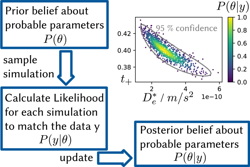
Updating prior knowledge given new evidence: this is the central idea behind any Bayesian algorithm. The preconditioning of estimation problems with prior knowledge enables Bayesian algorithms to require far fewer data points than empirical approaches. Some standard textbooks for Bayesian inference are References 42, 43, 44.
„Probability“ in the Bayesian context describes the level of uncertainty in the data rather than randomness. The result of any Bayesian algorithm is a probability distribution providing a range of estimates with their respective „probabilities“ to be the correct estimate. The estimated probability distribution also includes information about how the estimated model parameters influence the measurement individually and collectively 42, 43, 44.
Here we describe the basic Bayesian algorithm, which we outline in Figure 2. Firstly, transform the prior knowledge about the range of probable model parameters into a probability distribution , called Prior or „belief“. Secondly, take random samples from the Prior and calculate the so-called Likelihood for each parameter sample. The Likelihood represents the „Likelihood“ for each model simulation to match the experimental data. A simple approximation for the Likelihood is a Gaussian distribution with the simulation-experiment agreement as its expectation value and some variance 17. Finally, multiply the Likelihood with the Prior and normalize the result into a probability distribution , called Posterior. The third step is eq. 2, called Bayes’ Theorem. Bayes’ Theorem ensures that the Posterior reasonably updates the prior belief about probable parameter candidates 42, 43, 44,
| (2) |
In the following, we abbreviate „parameter“ as and „data“ as , as shown in Figure 2. Bayes’ Theorem then reads as .
The performance of a Bayesian algorithm crucially depends on the quality of the Likelihood approximation. A rough approximation of a Likelihood with a Gaussian 17 might lead to slow convergence or wrong estimates. And in the case of 1D+1D models without analytic solutions, a better Likelihood cannot be derived. However, the approximation that the Posterior is Gaussian is usually justified if the estimated parameters are identifiable from the data, given the Central Limit Theorem 42, 43, 44.
Likelihood-Free Inference (LFI), also called Approximate Bayes-
ian Computation (ABC), is a class of algorithms that approximate the unknown Likelihood from model evaluations. The shape of the Likelihood in LFI algorithms results from a Machine Learning procedure on simulated data samples, e.g., Cross-Validation 45. Instead of a Likelihood, LFI algorithms only need to know the discrepancy measure between a simulated measurement and an experiment. The added flexibility enables one to try out different models freely 46.
In contrast to DKFs, the discrepancy measure in LFI algorithms may encompass the whole experimental data rather than only one point in a time series at a time. The difference to MCMC methods such as the Metropolis-Hastings algorithm used by Aitio et al. 17 is that the quality of parameter guesses is judged by the approximated Likelihood rather than by the Posterior. Using the Posterior like Metropolis-Hastings may result in confirmation bias since it mixes the Prior into evaluating the quality of parameter fits.
The following sections present the two LFI algorithms we employ to minimize the required number of model simulations. Despite the improved generality and accuracy of our approach, we achieve a reduction rather than an increase in computational load compared to Metropolis-Hastings.
Expectation Propagation
Expectation Propagation (EP) was developed by Minka in his PhD thesis 47 and later revisited in a paper 48. EP has uses for training neural networks 49, object detection 50, speech recognition 51, and signal processing 52. We present Barthelmé et al.’s adaptation of EP to Likelihood-Free Inference (LFI) 37 using BOLFI as LFI algorithm (see Subsection Bayesian Optimization (for Likelihood-Free Inference) for BOLFI). For further reading, we recommend the general introduction to EP in 53, Chapter 3.6.
The great advantage of EP for LFI is splitting the data into multiple segments or discrete features. These features give the sampling algorithm within EP the more straightforward task of matching one part of the data at a time.
EP is proven to work accurately and efficiently based on its two core principles. First, the moments of the approximated Posterior converge to the moments of the actual Posterior. Examples of moments for probability distributions are the expectation value and the variance. Formally, moment-matching is only guaranteed if Posteriors get selected from an exponential family. Further details are summarized in the SI Section LABEL:SI-sec:expfam.
Second, EP efficiently optimizes multiple measurement parts together by iterating through them. From now on, we call these measurement parts „features“ and denote them with . EP searches the optimal parameter set for each feature in the range of probable candidates for the other features. Examples of possible features range from measurements in time to characteristic values, like decay rates.
The user sets up EP with the following two inputs 37. One is a functional definition of the features in simulation and data, which defines the cost function. The other is a Prior , which represents the initial belief for every vector of parameter values and defines the „initial value“ of the Bayesian algorithm. Additionally, one may pre-define the Likelihood sites for each of the features, but for initialization „uninformative Priors“ are appropriate. The EP algorithm then expresses the Posterior as the product of the Prior and each Likelihood site, as shown in eq. 3.
| (3) |

The procedure for EP 37 factorizes the simulation and data into individual features. EP then iterates through all features multiple times. For each feature, BOLFI optimizes the model parameters to fit this feature. The result of BOLFI is a more precise probability distribution of the model parameters. EP utilizes this result to update its distribution of probable model parameters for all features. EP uses the new Posterior as input for next feature optimization.
The algorithm of EP 37 iterates through the features of the whole data until a stop criterion is met, as shown in Figure 3. After initialization of the current Posterior with the Prior and the initial Likelihood sites, there are four steps in each iteration. Firstly, produce a „Pseudo-Prior“ by omitting the corresponding Likelihood site from the current Posterior. Secondly, use an LFI algorithm like BOLFI to compute an approximation to the Likelihood of the selected feature. We introduce BOLFI in Subsection Bayesian Optimization (for Likelihood-Free Inference). Thirdly, produce a „Pseudo-Posterior“ by replacing with the updated . BOLFI basically takes the Pseudo-Prior as its Prior, approximates a Likelihood, and outputs the Pseudo-Posterior as its Posterior, i.e., the product of Pseudo-Prior and approximated Likelihood. Finally, replace the current Posterior with the Pseudo-Posterior for the next iteration and start the next iteration.
There is one caveat inherent in the capability to run multiple loops through all features. At the step where replaces , more precisely a projection of replaces . The projection to a certain type of probability distribution ensures that the replacement results in a Pseudo-Posterior that retains its type of probability distribution. In our case, all involved quantities , and , and hence, , are normal distributions. Any multi-modality in before projection gets lost and only results in a wider normal distribution after projection that smooths over the multiple modes. In the algorithm description above, we omit dampening for clarity. With a dampening parameter , dampening is introduced to EP by linearly interpolating between prior to each site update and in terms of their so-called „natural parameters“. 37 We show the detailed formula in the SI Section LABEL:SI-sec:EP.
The advantage of subdividing the discrepancy between experiment and simulation into features is the reduced number of simulations needed for convergence. Any LFI algorithm must decide which of the sample simulations it should include in the Likelihood approximation. The more complex the Likelihood is, the more samples the LFI algorithm ultimately discards due to the so-called „curse of dimensionality“. With each additional „dimension of complexity“, the computational effort to deal with it grows exponentially. By „dimension of complexity“, we refer to the effective dimension of the information in the data. For example, suppose a set of fitting functions describe the data up to noise. Then, the information contained has a dimension not larger than the number of fit parameters rather than the number of data points. Using a subset of the whole discrepancy with a lower dimension gives a much higher chance of any random sample being close to the optimum of this subset 37.
The sequential handling of the features further reduces the computational complexity. Each fitted feature, i.e., updated , preconditions the estimation task much like the Prior does at the beginning of every Bayesian algorithm. Hence, EP takes no unnecessary samples that contradict an already fitted feature. This preconditioning is most efficient when the features are uncorrelated, which gives an upper limit on the sensible number of features.
Minka 47 has proven that EP converges in the sense of minimizing the so-called Kullback-Leibler Divergence (KLD). KLD is not an actual distance metric for distributions, but its second derivative gives a pragmatic approximation of the usually used Fisher Information Metric (FIM) 54. EP converges on the mean of the posterior with quadratic speed when the posterior tends to a normal distribution, as stated in Barthelmé et al. 37. Here, is the total number of simulation samples.
Bayesian Optimization (for Likelihood-Free Inference)

Bayesian Optimization for Likelihood-Free Inference (BOLFI) was developed by Gutmann et al. 38. Applications of their algorithm include the fields of cosmology 55, ecology 56, genetics 57, and neurobiology 58. We use an implementation of BOLFI by Lintusaari et al. in the software ELFI 59. For further reading, we recommend the introduction to BOLFI in 60. To the best of our knowledge, we are the first to combine BOLFI with Expectation Propagation.
Bayesian Optimization takes the idea of preconditioning an estimation task with a Prior one step further: this class of algorithms utilizes each sample to optimize the choice of the following sample. This short-circuiting of the usual Bayesian recipe allows for the active selection of the most informative following sample, where standard Bayesian algorithms draw samples randomly. Figure 4 visualizes how BOLFI „explores“ the parameter search space before „exploiting“ the region where BOLFI expects the optimal parameter set. A sample is chosen by minimizing its „acquisition“ function in eq. 5. To this aim, a Gaussian Process is trained on the preceding simulation samples and acts as a fast surrogate for the intractable discrepancy-parameter relationship to enable this minimization.
BOLFI works best for low sample numbers. This is because it involves the inversion of a matrix with rank equal to the sample size at each sample. Expectation Propagation helps in this respect as it keeps the sample size small. Each feature update resets the samples to 0 and provides a more precise Prior for the next iteration. While this resolves the most significant weakness of BOLFI, it requires that the form of the current Posterior does not change over multiple site updates. Here, we limit ourselves to Gaussian distributions. The transformations can limit the parameters to positive numbers by taking the logarithm or to an interval by taking the tangent. Please note that any proper probability distribution can be optimized with BOLFI.
For each feature with index , the algorithm of BOLFI 38 starts with a user-defined number of (quasi-)random samples from the Prior. To achieve optimal integration efficiency, these samples stem from a Sobol sequence 61. These samples and the deviations between simulation and experiment constitute the data that BOLFI trains a surrogate function on. Here, is the current feature of the experimental data and is the simulated feature for the parameter set . For illustration, Figure 4 shows as blue dots over , where the blue line labelled „discrepancy“ would be that surrogate function.
The training points are assumed to follow a Gaussian Process with parabolic mean function. From this model, BOLFI applies a filter to this Gaussian Process to calculate the approximation to the model-simulation discrepancy ,
| (4) |
where is adjusted automatically. We show the derivation of this Posterior in the SI Section LABEL:SI-sec:BOLFI.
and constitute a differentiable surrogate function for the intractable model-simulation discrepancy function
. Following the initial regression to the Sobol quasi-random samples, further samples are generated from the surrogate in eq. 4 in the following manner, called „lower confidence bound selection criterion“ 38. The next sample gets taken as the minimum value of the so-called acquisition function
| (5) |
where is a sufficiently large scaling factor that grows logarithmically with . 38 Figure 4 shows a visualization of the acquisition function, where is represented by the blue line and is the width of the grey-shaded region around that blue line, while the orange line represents the acquisition function itself.
The minimum of the acquisition function approximates the parameter set with the highest chances of generating a simulation closest to the experiment. Hence, BOLFI generates samples sequentially and optimally to minimize the remaining uncertainty in the Likelihood estimation.
After finishing the acquisition of samples, the final surrogate in eq. 4 forms the basis for the Likelihood approximation, as shown in Figure 5. In the Likelihood-Free Inference (LFI) framework, the approximation to the Likelihood is the probability that the discrepancy surrogate falls below a threshold value :
| (6) |
The threshold value is arbitrary in most LFI algorithms, but BOLFI infers it from the surrogate itself as . With the probability density function of the Gaussian surrogate, can be calculated as
| (7a) | ||||
| (7b) | ||||
where is the cumulative distribution function of a standard normal variable,
| (8) |
Simultaneously regressing and sampling from the sampling distribution reduces the number of required samples by several orders of magnitude. 38
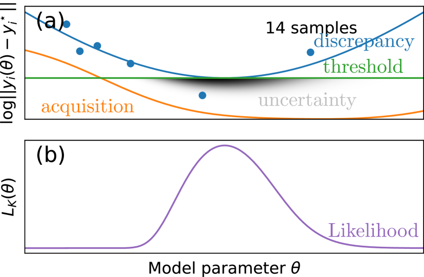
Validation of EP-BOLFI performance
| true | initial std. | Aitio et al. (MCMC), | EP-BOLFI | EP-BOLFI | EP-BOLFI | |
|---|---|---|---|---|---|---|
| parameter | value | deviation | simulations | sim. | sim. | sim. |
| / | ||||||
| / - | ||||||
| / | ||||||
| / | ||||||
| / |
Our reference for state-of-the-art automated battery model parameterization is the work of Aitio et al. 17. They create two types of synthetic data with an SPMe model, multimodal sinusoidal excitations at eleven SOCs denoted „excitation-point case“ and a discharge with a superimposed small unimodal sinusoidal excitation denoted „wide-excursion case“. Aitio et al. fit five parameters with an MCMC algorithm: the electrolyte and solid diffusivities , , the cation transference number , and the variance of the white noise superimposed on the synthetic measurement. In the wide-excursion case, MCMC fits the parameters nicely. However, the MCMC algorithm finds a wide range of inconsistent values in the excitation-point case 17.
We apply our EP-BOLFI algorithm to the same synthetic data with the same SPMe model as Aitio et al. 17. Aitio et al. take the -distance of the voltage as the cost function. For the EP-BOLFI algorithm, we preprocess the voltage response and define features. For the excitation-point cases, we perform a Fast Fourier Transform on the current input and voltage output to calculate the impedance for each mode as features. For the wide-excursion case, we use the -distances of four voltage curve segments as features.
The results for the wide-excursion case are shown in Table 2. We observe that EP-BOLFI reaches a similar accuracy to that in Aitio et al. 17 with about 12 times less simulations, depending on the model parameter. Between and simulations for EP-BOLFI we observe an order of magnitude increase in accuracy, and at simulations all but are as accurately or even more accurateley estimated as by MCMC.
The comparison of EP-BOLFI to MCMC in Aitio et al. 17 for the excitation-point case is shown in the SI Table LABEL:SI-tab:comparison. Across all excitation points, EP-BOLFI with simulations vastly outperforms the MCMC approach in terms of stability and accuracy.
EP has the potential to deal with the data at all excitation points at once. Hence, we perform an additional experiment, collating the four excitation points 1, 2, 3 and 7 with the smallest uncertainties. While that leads to overfitting, the number of simulations required to reach convergence even shrinks to . This demonstrates that the computation time of EP scales favourably with the dimension of the data 37.
Experimental
Experimental setup and a priori known parameters
| parameter | source | value |
|---|---|---|
| A priori assumed parameters | ||
| value for NMC-111 62 | 1.07 | |
| value for graphite 62 | 10.67 | |
| symmetry assumption | 0.5 | |
| Subsection Measurement of the OCV curves | ||
| GITT measurement 63 | [0.0, 1.0] | |
| our GITT measurement | [3.0, 5.0] | |
| scaling factor, cf. eq. 9 62 | ||
| scaling factor, cf. eq. 9 62 | ||
| scaling factor, cf. eq. 9 64 | ||
| scaling factor, cf. eq. 9 64 | ||
| Subsection Parameters fitted with EP-BOLFI | ||
| EP-BOLFI fit | TBD | |
| EP-BOLFI fit | TBD | |
| EP-BOLFI fit | TBD | |
| EP-BOLFI fit | TBD | |
| EP-BOLFI fit | TBD | |
| EP-BOLFI fit | TBD | |
| EP-BOLFI fit | TBD | |
The full cell GITT data got measured at BASF. Here, we list the parameters known before starting our estimation algorithms, following the checklist in 65. The only points in that checklist we do not fulfill are „specifications of used materials“ and „coulombic efficiency“.
The GITT measurement protocol consists of repeating sets of -, -, - and - pulses with occasional - pulses each 25% SOC (State-Of-Charge). corresponds to a theoretical capacity of . The rest periods at zero current between the pulses were , with the exception of the pulses, which were enclosed in rests. The GITT experiment was conducted at 25 °C. The minimum and maximum operating voltage of the cell are and , respectively. The GITT data spans from SOC 25% to 100%, i.e., 25% discharged to 100% discharged.
The cell contains the following materials. The negative electrode mostly consists of graphite with 95.7% active material and is slightly overbalanced. The separator is Celgard 2500 with thickness. The positive electrode is 94% NCM-851005 with 3% Solef 5130, 2% SFG 6L and 1% Super C 65. The electrolyte is LiPF6 in EC:DEC 3:7 with 2% VS as SEI former.
Here, we list the geometric parameters and the electrolyte properties. The cell is a square pouch cell. The cross-sectional areas are , , and for the negative electrode, separator, and positive electrode, respectively. The porosities are roughly 0.27, 0.55, and 0.29 for the negative electrode, separator, and positive electrode, respectively. The porosities of the electrodes were approximated by comparing their density with the bulk densities of graphite at and NCM-851005 at (times 94%), respectively. The porosity of the separator and its Bruggeman coefficient of 3.6 were taken from Patel et al. 66. The thicknesses of the electrodes are and for the negative and positive electrodes, respectively. Both thicknesses were calculated from densities and areal mass loadings, i.e. the mass of active material per cross-sectional area of the respective current collector. The areal mass loadings of the negative and positive electrode are and , respectively. Thus, the electrolyte volume is about and the volumetric ratio of electrolyte to active material is about 0.737. The electrolyte has cation transference number , thermodynamical factor , diffusivity , and conductivity . We take the a priori electrolyte parameters from Nyman et al. 67, even though they characterized EC:EMC 3:7, not EC:DEC 3:7. We neglect this disparity, since our focus is to demonstrate our parameterization procedure. We consider the cation transference number unknown with known error bounds and tie the thermodynamical factor to it as .
At this point, we fixed most parameters. We discuss the remaining unknown parameters listed in Table 3 in the next subsections. We shortly discuss the few unknown parameters with negligible impact here. The electronic conductivities of the electrodes are from Danner et al. 62; there, the electrode materials were graphite and NMC-111. We accept the potential error due to the different materials, since the electronic conductivities typically only account for a static IR drop of up to at current . The charge-transfer coefficients, also known as asymmetry factors, are set to , i.e., we make the standard assumption that the charge-transfer reactions are symmetric.
Measurement of the OCV curves
The Open-Cell Voltage (OCV) has by far the most significant effect on the overall operating cell voltage, typically about to . The minor voltage losses described by the equations in table 1 are due to the limiting transport processes and reactions the so-called „overpotential“. The overpotential is typically around . Hence, before we analyze cell processes via the overpotential, we need to know the OCV of the cell with high precision 68.
The most precise measurement of the OCV is possible with GITT, with a voltage error of 63. Still, measurements at low constant current get often misused as „quasi-OCV“ (qOCV) measurements 30, 34. Chen et al. 31 demonstrate how constant-current curves exhibit significant deviations from OCV at high or low charge and between voltage plateaus, even at low current. Hence, we do not use qOCV measurements.
We use the physics-inspired OCV model of Birkl et al. 63, as it assigns an SOC range to incomplete OCV data in an informed and automatic way. This SOC range will approximate the maximally lithiated and de-lithiated states of the positive electrode at SOCs 0 and 1, respectively. We denote that SOC range as „positive electrode SOC“ or . Likewise, we refer to the maximally lithiated and de-lithiated states of the negative electrode when we assign the „negative electrode SOC“ or .
We fit the OCV curve of the positive electrode given the OCV curve of the negative electrode in Subsection Extracting positive electrode OCV from full-cell GITT. The maximum intercalation concentrations were fitted to the CC-CV and GITT data at the same time.
Parameters fitted with EP-BOLFI

We now have seven model parameters of interest that we can fit to the GITT data, summarized in eq. 9. These are the model parameters that appear independently from unknown properties in our physics-based model,
| (9) |
For simplicity, we assume that these parameters are independent from electrolyte concentrations and location within the cell. We ignore the concentration dependence of the cation transference number 69. We assume that the Bruggeman coefficients are spatially constant. Spatially and concentration resolved measurements are required to parameterize these heterogeneities.
GITT measurements give us information about SOC dependence. The functional form of the exchange-current density
is an active topic of research 70, 71, 72, 73. Likewise, the active material diffusivities depend on electrode SOC 74. Hence, there are three parameters of interest that do not depend on SOC, namely , , and , and four that do depend on SOC, namely , , and . Therefore, we fit all seven parameters of interest in eq. 9 once to a pair of GITT pulses with different C-rates. Then, we hold the three SOC-independent parameters constant, and fit only the four SOC-dependent ones to all other GITT pulses.
We also miss the geometric parameters for the electrode particles to correctly scale the active material diffusivities and the exchange-current densities . However, their absolute values can be corrected when the specific surface areas and particle radii get measured. Without loss of generality, we assume the specific surface area 64. Analogously, the particle radii are just a scaling factor in our model. We arbitrarily take the particle radii from a battery of Danner et al. 62.
For Expectation Propagation, we reduce the experimental data to discrete features as visualized in Figure 6. The five features we fit are the voltage directly after the current has been shut off (concentration overpotential), the relaxation times during the discharge pulses, the ohmic voltage drop, and the GITT and ICI (Intermittent Current Interruption) square-root slopes 75 during discharge pulses and rest periods, respectively. We use the following fit function to obtain the square-root slopes and the offsets of the square-root segments :
| (10) |
where refers to the start of the current pulse or the start of the rest phase. The square-root function fitted to the current pulse gives the ohmic voltage drop as and the GITT square-root slope as . The square-root function fitted to the rest phase gives the concentration overpotential as and the ICI square-root slope as . To get the relaxation time , we use the following fit function on the current pulse:
| (11) |
where refers to the start of the current pulse. While our current pulses are too short to fulfill the requirements for ICI as an analytical formula, we will later see that our „incomplete“ ICI square root slopes still give valuable information. We omit the exponential relaxation at rest as a feature since it is difficult to fit uniquely 76, 69. This is discussed in Section Discussions. We omit and from the exponential fit function in eq. 11 as features, as they are less consistently fitted than the concentration overpotential, which contains much of the same information.
The analysis of GITT and ICI with approximate formulas introduces some inaccuracy as discussed by Geng et al. 77. EP-BOLFI fits the whole DFN model directly to the experimentally observed square root slopes. A detailed discussion for the complementary relevance of both GITT and ICI features is performed in the SI Section LABEL:SI-sec:features. We emphasize that one might also use simple time segments of the data with their -distance as features for EP-BOLFI if no better preprocessing step is known. The features we chose have less interdependence than -segments, accelerating the computations and making the results more interpretable. As we can see in Figure 6, we capture the main information of the raw voltage curve in the five features.
We choose normal distributions for the Bruggeman coefficient priors and the cation transference number, and log-normal distributions for the priors of all other parameters of interest. We motivate the log-normal distributions with the Arrhenius relation: reaction rates and diffusivities may be modelled as a reaction following an Arrhenius relation, and hence are log-normally distributed if the corresponding activation energies are normally distributed. In the spirit of Laplace approximations 78, a good approximation of the true distributions close to the true estimate is sufficient, even for global optimization. The bounds of the prior and posterior 95% confidence intervals and the most likely estimates are listed in Table 4.
Computational details
We employ the helpful checklist from Mistry et al. 79 to ensure that we include every aspect of sensitivity of numerical inputs. The filled-in checklist is in the SI Table LABEL:SI-tab:checklist in the SI Section LABEL:SI-sec:checklist.
We discretize the 1D+1D model equations in table 1 with Spectral Volumes 80 and solve them with CasADi 81 interfaced through PyBaMM 82. Compared to Finite Volumes and the ode15s solver in MATLAB, our simulations run 20 times faster. The Spectral Volumes mesh is of order 8 in the electrolyte and the negative electrode particles and of order 20 in the positive electrode particles. For the electrolyte mesh, 2 Spectral Volumes are in the negative electrode, and 1 Spectral Volume each is in the separator and the positive electrode. We check for mesh independence by running a simulation with orders 16 and 40 instead of 8 and 20, respectively: the features change by no more than 0.2%. The timesteps are at most , and reducing them to at most changes the features by no more than 2%.
Whenever we fit a parameterized function to data points, we use the trust-region algorithm for constrained optimization implemented in SciPy. The OCV model 63 we use gives the electrode SOC as a function of its OCV. Since the 1D+1D model equations in table 1 require the inverse function, we invert OCV model fits numerically and fit a spline to the inverse. Compared to direct spline fits to data, we retain the model-informed smoothing of the data and the estimation of the SOC range.
Our algorithm can consider the uncertainties of all model parameters if the simulator function randomly samples them. Hence, we included the uncertainties of the SOC-independent fit parameters , and in the parameterization of the individual GITT pulses.
For the initial fit of the SOC-dependent parameters, we choose the final GITT pulse in the dataset. The final GITT pulse corresponds to the most extreme SOC and, therefore, the largest overpotential, ideal for an initial fit. The SOC-dependent parameters and vary over two to four orders of magnitude, respectively. To allow for this parameter variability from one GITT pulse to the next, we magnify the error bars of the SOC-dependent parameters of one fit before we use them as Prior for the next fit. We limit the lower and upper bounds the priors could take to for the exchange-current densities and to [1e-14, 1e-10] for the electrode diffusivities. This limiter prevents the fit parameters from diverging into regions with infinite exchange-current density or instant diffusion. The error bars are then magnified to span at least half of the lower and upper bounds in the log scale.
We fit the seven parameters of interest in eq. 9 to GITT data in Subsection Extracting model parameters with EP-BOLFI from GITT with our EP-BOLFI algorithm. We estimate parameters with warm-up samples and samples in total for BOLFI for each individual feature update, respectively. The pseudo-posteriors are estimated with an effective sample size of for , respectively, by the No-U-Turn-Sampler 83, a Markov-Chain Monte-Carlo sampler implemented in ELFI 59. We set up 4 EP iterations in both cases. We set the EP dampening parameter such that the total dampenings at the end are .
For validation of our novel EP-BOLFI algorithm, we repeat the estimation procedures with one difference. We replace the measured data with synthetic simulated data for the most likely fit parameters. The better a given parameter is identifiable from the features, the closer the verification run would be to the first results. With this validation, we also make sure that EP-BOLFI converged, such that we can be sure that invisible non-identifiability issues arise purely from model and data.
The total time for the estimation of seven parameters of interest with simulations on our office PC with an Intel Core i7-6700 at 4.00 GHz x 8 is about 20 hours. Of that, roughly twelve hours is the simulation time for simulations of two GITT pulses. The total time for the estimation of the four SOC-dependent parameters of interest with simulations for each pulse is about 120 minutes on our PC. Of that, roughly 80 minutes is the simulation time for simulations of one GITT pulse.
Results from full-cell GITT data
Before we describe the application of EP-BOLFI to GITT data, we have to identify the OCV of the positive electrode in Subsection Extracting positive electrode OCV from full-cell GITT. The application of EP-BOLFI is then presented in Subsection Extracting model parameters with EP-BOLFI from GITT.
Extracting positive electrode OCV from full-cell GITT

We want to obtain the open-circuit voltage (OCV) of the positive electrode. Since we do not have half-cell data, our estimation relies on our approximate knowledge of the OCV of the negative electrode 63.
As a first step, we determine the cell balancing, i.e., the negative electrode SOC as a function of the positive electrode SOC. To find the cell balancing, we determine an approximate second derivative of from the data. We obtain that by shifting the CC curves by the CV step against each other, adding them, and subtracting the GITT curve two times. The derivation of this preprocessing step and the utilized data are laid out in the SI Section LABEL:SI-sec:OCV_preprocessing.
We compare the second derivative of to that of a known graphite OCV curve 63 in the SI Section LABEL:SI-sec:OCV_preprocessing. Though being a rough approximation, we can identify the peak positions of the second derivative. We find that the negative electrode SOC ranges from 3% to 84% over the SOC range of the positive electrode.
Taking into account this cell balance, we obtain from the sum of and the cell OCV from GITT data in Figure 7. We find that the cell capacity is . The OCV model of Birkl et al. 63 with eight phases gets fitted to the SOC range and we trust its extrapolation to the SOC range . We ignore OCV hysteresis effects 63 and only consider the discharge direction from now on.
Extracting model parameters with EP-BOLFI from GITT
| Parameter | prior bounds | posterior estimate |
|---|---|---|
| [1.0, 100.0] | 12.3, [10.2, 14.8] | |
| [1.0, 100.0] | 36.3, [29.9, 44.0] | |
| [1e-14, 1e-10] | (1.19, [0.82, 1.73])e-11 | |
| [1e-14, 1e-10] | (0.82, [0.56, 1.22])e-11 | |
| [0.2, 0.4] | 0.349, [0.343, 0.355] | |
| [1.8, 4.2] | 2.72, [2.64, 2.81] | |
| [1.8, 4.2] | 3.06, [2.99, 3.13] |
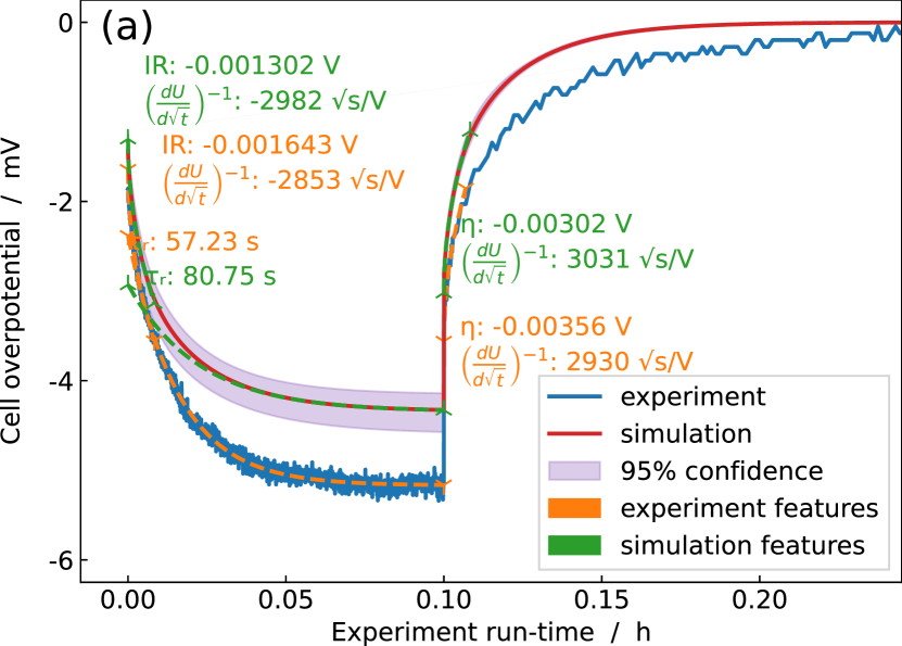

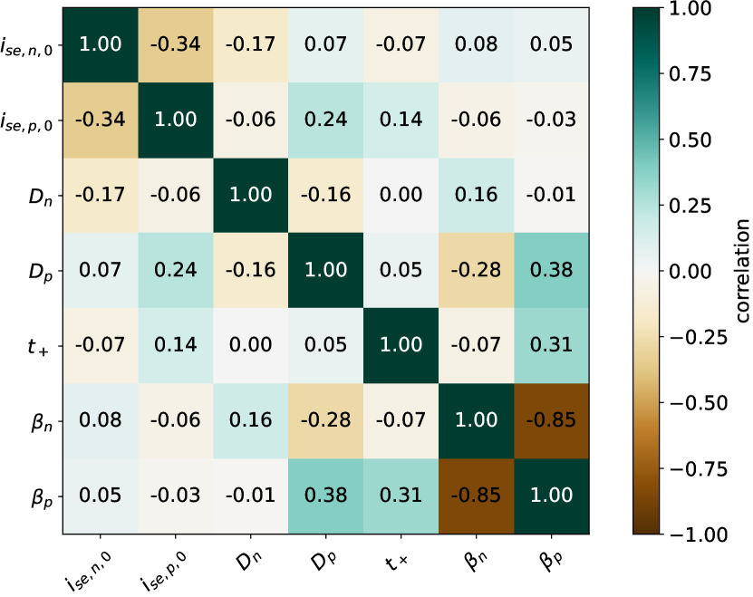

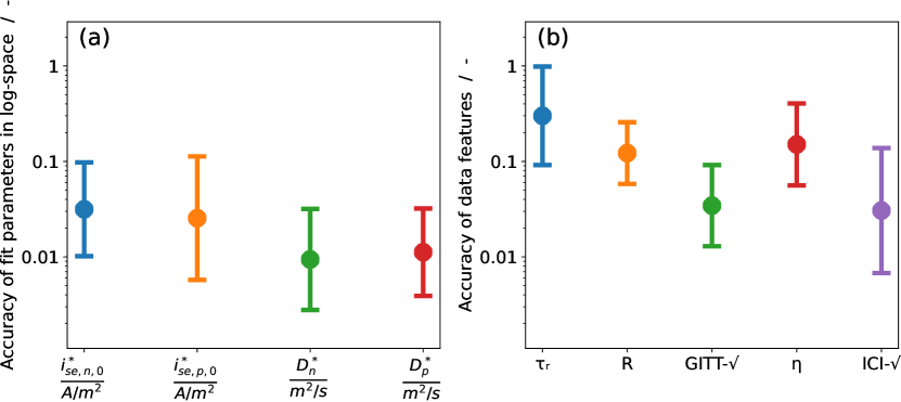
With the procedure laid out in Subsection Computational details, we fit seven parameters to GITT pulses 66 () and 67 () in the data. We choose these pulses since the OCV curves of both electrodes have significant gradients there, which improves the sensitivity of our experimental data to electrode diffusivities 75. Our prior bounds are based on the LiionDB database 85 and an order-of-magnitude estimate of the exchange-current densities and active material diffusivities. We show the fitting results as estimates and 95% confidence intervals in Table 4.
In Figure 8, we depict the five fit features in the experiment and how we predict them in the simulation. The good agreement between features in simulation and data at low and high current verifies our optimization. The square-root GITT and ICI features have an excellent agreement. However, there is a significant difference in fit quality between low () and high () current for the exponential relaxation. We discuss that electrode heterogeneity can explain this mismatch (see Section Discussions). We find direct relationships between features and parameters below; thus, the excellent fit of most of the features gives insights on its own. Figure 8a is a good example to illustrate our featurization approach. If we had optimized the model for the time series, the simulation would cut across the voltage measurements, matching neither short-term nor long-term processes in the battery.
We now discuss the correlation matrix, i.e., the covariance matrix normalized by the variances. In Figure 9, the correlation matrix indicates how a parameter change affects the estimates of the other parameters. Each matrix entry shows how the (lack of) knowledge of some parameters influences the accuracy of the other parameters. Correlations close to 0 indicate that the two parameters are not coupled in the data as interpreted by our model. Note that the two exchange-current densities are correlated with each other in our full cell examination. We see correlations between the SOC-independent model parameters and the SOC-dependent ones, especially between the diffusivity of the positive electrode and both Bruggeman coefficients. We rerun the estimation procedure twice with different initial random seeds to validate that these correlations are consistent properties of model and data rather than numerical artefacts. The corresponding data are in the accompanying GitHub repository. These correlations demonstrate the benefit of estimating all seven parameters together, namely that we obtain a consistent parameter set.
Next, we fit all GITT pulses with only the SOC-dependent four parameters , , and under consideration of the remaining uncertainty of , and . In Figure 10, we plot the optimal estimates and error bars corresponding to one standard deviation of the logarithmic parameters as a function of electrode SOC. Please note that we define „electrode SOC“ by the theoretical minimum and maximum lithiation of an electrode. The error bars in Figure 10 show us how precise the parameters are estimated in each GITT pulse.
We compare the exchange-current densities in Figure 10a and Figure 10b with the standard SOC-dependence of the Butler-Volmer rate in eq. 1h 71. One reason for the large error bars is that the two exchange-current densities primarily act as interchangeable resistances. In the SI Figure LABEL:SI-fig:joint_resistance, we plot their joint resistance. Since it is not much smoother and has large error bars, we can conclude that there are more identifiability issues than just the interchangeability of the two exchange-current densities. The low identifiability is not surprising, as GITT was not designed with measuring exchange-current densities in mind. Both exchange-current densities are visible in measurements on much smaller timescales 6 than the GITT pulses used here, which means that they mostly collectively show up as a contribution to the ohmic drop.
The diffusivities in Figure 10c and Figure 10d are smoother functions of SOC. The error bars are still more prominent than in a half-cell setup, for which GITT was initially designed 5. We attribute the larger error bars to a limited discernability of the two electrodes in the data. To discuss the results for , we plot the results of the analytic formulas for the GITT and ICI methods 75 for in Figure 10c. We show these formulas in the SI Eq. 8.37. These formulas neglect the influence of the negative electrode and the electrolyte; hence, there is no equivalent formula for . We instead compare with a measurement by Schmalstieg et al. 84.
The results for in Figure 10c have fairly small error bars and seem to be rather constant, in contrast to the analytical GITT and ICI formulas. The analytical formulas have especially large deviations from our results in the regions around and . At the positive electrode OCV curve has a very flat plateau that impedes the analytic formula and introduces large uncertainty to it. At the low diffusivity of the negative electrode at corresponding may disturb the analytical formulas. EP-BOLFI, instead, produces consistent estimates for both diffusivities and can even distinguish between the two electrodes. Hence, the prediction of the uncertainty displayed in Figure 10c gives us further information about the completeness of the experimental data and the predictability of the model parameters.
The results for in Figure 10d exhibit slightly smaller error bars than those for and reproduce the literature data of Schmalstieg et al. 84 well. They observe the same shape of the diffusivity curve in a half-cell with graphite, especially the dip around . Kang et al. 86 perform a detailed analysis of the possible sources of uncertainty, such as the duration or intensity of the current pulses.
Please note that we can not determine the absolute magnitude of the estimates for and , as they depend on the unknown particle radius and , respectively. We emphasize that we can identify and separately, as indicated by their weak correlation in Figure 9 and their agreement with expected behaviours. We achieve this even though we measured a full cell and do not know the electrolyte properties perfectly.
In Figure 11a we verify how reliable our parameterization result is. For this purpose, we create synthetic data from a DFN model with the parameters we fitted to the experimental data (see Figure 8). We apply EP-BOLFI to this SOC-dependent synthetic data in a verification run. We depict here the relative deviation between the true and estimated parameters in this verification run. As the fitted probability distributions are log-normal, we observe the relative deviations on a log-scale. We confirm that the solid diffusivities are identifiable within 1% accuracy. Notably, the exchange-current densities show a much larger variability in accuracy, matching their erratic behaviour in 10ab. We conclude that the diffusivities in Figure 10cd can be trusted at most SOC, while the exchange currents in Figure 10ab are not clearly identifiable from GITT. We also verify that the model justifies the limitation to a Gaussian Posterior with only one mode since multiple distant sets of equally optimal parameters would result in far poorer accuracy.
In Figure 11b, we verify that the parameterization accurately reproduced the experimental data. For that, we collect the deviations between features in the experimental data to the features in the fitted simulated data. We see that all features were fitted well except for the exponential relaxation time . We conclude that is an unreliable feature in our GITT dataset with the DFN model.
In the SI Section LABEL:SI-sec:sensitivity, we perform a complementary sensitivity analysis on the DFN model at the fitted parameters at each GITT pulse. Based on these sensitivities, we can identify parameters that appear to be fitted well in Figure 11a, but depend on unreliable features in Figure 11b. As we can see in the SI Figure LABEL:SI-fig:sensitivities, and both depend on all features but the ohmic resistance, with being more sensitive to the concentration overpotential than . We find that all four SOC-dependent parameters also have a consistently high sensitivity to the exponential relaxation time , which we just ruled out as a reliable feature. Despite that sensitivity, EP-BOLFI automatically ignored in favour of fitting the parameters more consistently with other features. We conclude that we can nicely estimate and accurately from our GITT dataset because they are sensitive to the square-root features and the concentration overpotential.
Discussions
We gain three benefits from our Bayesian method, EP-BOLFI. The first benefit is universality; treating the model as a black box allows us to change the equations and fit parameters arbitrarily. The second benefit is global optimization, i.e., the thorough exploration of the range of feasible parameters. The third benefit is that we consistently estimate both the fit parameters and their uncertainty with only one algorithm.
State-of-the-art battery parameterization most often requires a complicated calculation of the parameter-output-gradient 18, 24. For example, Sethurajan et al. 18 and Zhao et al. 24 conduct microscopic imaging of electrolyte concentration profiles. They then apply gradient-based iterative optimization to diffusion equations to extract electrolyte properties. While this specialization produces fantastic results, adapting their algorithm to other battery parameters or differential equations would warrant a new paper. With our algorithm, you only need to update the simulator and the feature definitions.
The „exploration“ aspect of BOLFI ensures that it evenly minimizes the remaining uncertainty across the whole parameter search space. A gradient-based approach would be limited to the estimate „closest“ to the initial guess. Repeating the gradient-based optimization from various starting points can alleviate this locality problem, but it quickly becomes infeasible with a growing number of estimated parameters.
The Bayesian analysis of Sethurajan et al. 18 and Zhao et al. 24 is preceded by a gradient-based optimization. EP-BOLFI is stable enough not to require this step, drastically cutting down on the implementation effort while incorporating a more expansive parameter space into the uncertainty estimate.
The comparable computation time for the simulations and the EP-BOLFI algorithm shows a considerable cost to optimizing the samples. Compared to Aitio et al. 17, we require at least 12 times fewer samples for the estimation of five parameters. Hence, we significantly reduce the computation time and enable the simultaneous estimation of more than four parameters.
The primary use of our technique is model parameterization, i.e., it tunes the model for predictive simulations, e.g., for a digital twin. Depending on the sophistication of the model, its parameters might be very close to the actual material properties. Thus, we may also characterize the battery non-destructively multiple times over its lifetime. Established characterization techniques usually require separate setups with Li-metal electrodes or destructive disassembly 5, 8, 31. Our results for are comparable to those of a half-cell GITT measurement 84, indicating that we extract the actual electrode property rather than some effective cell parameter.
We believe that directly fitting continuum models includes significant coupled effects that analytic approximations can not describe. For example, the analytical formulas for GITT date back to 1977 5, and are only accurate for electrodes whose Open-Circuit Voltage (OCV) is locally describable by a Nernst equation. Modern electrode materials feature OCV curves with plateaus and kinks that severely impact GITT measurements, as we saw in Subsection Extracting model parameters with EP-BOLFI from GITT in Figure 10c. Our approach is less sensitive to this problem, as seen in Figure 10c.
Our focus is salvaging CC-CV and GITT measurements and other organically grown measurement protocols such as WLTP since they constitute most of the experimental data available. Hence, our algorithm can also deal with raw data that is simply divided into multiple time segments, where their respective -distances between measurement and data would be the features. Such a segmentation reproduces the total -distance while utilizing the benefits of Expectation Propagation. The result is a better global -fit with less computational cost. This flexibility alleviates the dependence on data that is generated specifically for optimal parameter estimation performance 87.
We can optimize a fitting procedure itself using the results of our algorithm. By studying the itemized correlation matrices for each feature, we can select the feature set with the clearest distinguishability between fit parameters. An analysis of the individual identifiability of each fit parameter is possible with either the diagonal of the covariance matrix or an interval analysis with the corresponding 95% confidence intervals.
The poor agreement between model and data exponential relaxation times at rest is likely due to the artificial homogeneity of the DFN model. The spatial heterogeneities of a battery cell significantly impact its performance and are best captured by microstructure-resolved modelling 88, 12. The link between exponential relaxation times at rest and heterogeneity has been discussed by Kirk et al. 89. They propose at least a multi-particle 1D+1D model, the MP-DFN, that incorporates the different length scales of the electrode particles.
Conclusion
Our newly developed algorithm EP-BOLFI is an optimizer that only requires the to-be-optimized model while minimizing the algorithm setup and the model evaluations. At the same time, the results of EP-BOLFI grant further insight into the data and the measurement uncertainty. EP-BOLFI and the data we applied it to are freely available. The GitHub repository containing the algorithm and the data is linked in Section Code availability.
We show that EP-BOLFI is more robust than MCMC, while simultaneously being an order of magnitude faster. The segmentation into expert-informed features allows the algorithm to reliably match the model to the parts of the data that it can actually reproduce. We successfully parameterize a DFN model to a real full-cell GITT experiment while treating the model as a black box. „Black box“ refers to the fact that EP-BOLFI does not require a pre-calculated gradient of the model-data discrepancy with the model parameters. Our results extract both electrode diffusivities, which would not be possible with the analytical GITT formula.
The non-destructive parameterization of models for the SEI 90, double-layers 91, and plating 4 might be possible with our algorithm. We expect to elucidate important correlations between these effects.
EP-BOLFI allows to combine different measurement techniques for parameterisation. For example, Electrochemical Impedance Spectroscopy (EIS) can distinguish processes occurring at different time scales like reaction kinetics. This is a deficiency of GITT, as shown in this article. EP-BOLFI could fit EIS and GITT measurements simultaneously and determine a greater parameter set.
An adaptation of our algorithm to faster simulators or more parallel processing power may swap out BOLFI for Robust Optimization Monte Carlo (ROMC) 92, implemented in ELFI 59. For fitting a large number of features, EP may be (partially) parallelized. The EP features can be updated iteratively or in parallel. But they can alternatively be updated in a in-between manner, where one can still reap some of the benefits of iterative preconditioning while utilizing more parallel processing power 37.
Code availability
The bytecode of the presented EP-BOLFI optimization algorithm and the code which we use to create the figures is available at the following GitHub repository:
https://github.com/YannickNoelStephanKuhn/EP-BOLFI.
The source code of EP-BOLFI will be available at that same GitHub repository at a later date. The experimental data is there as well in the „Releases“ section.
| Parameters | Units | Description | Non-dimensionalization |
| Spatial and temporal discretization | |||
| Thickness of the cell | |||
| Thickness of cell component | |||
| Spatial coordinate through the cell | |||
| Radius of electrode particles | |||
| Radial coordinate through a particle | |||
| Discharge timescale | |||
| Time since beginning of experiment | |||
| Electrolyte variables | |||
| Electrolyte concentration | |||
| Electrolyte potential | |||
| Electrolyte ionic current density | |||
| Molar ionic flux | |||
| Electrode variables | |||
| Concentration of intercalated lithium | |||
| Electrode potential | |||
| Electrolyte-Electrode interface reaction variables | |||
| Electrode electronic current density | |||
| Reaction overpotential | |||
| Intercalation reaction current density | |||
| Operating conditions | |||
| Current density applied to the battery | |||
| Temperature of the cell | |||
| Electrolyte parameters | |||
| Electrolyte diffusivity | |||
| Electrolyte ionic conductivity | |||
| – | Cation transference number | – | |
| – | Thermodynamic factor | – | |
| Electrode parameters | |||
| – | Electrode porosity | – | |
| – | Electrode Bruggeman coefficient | – | |
| Electrode active material diffusivity | |||
| Electrode electronic conductivity | |||
| Electrode surface area to volume ratio | |||
| Open-Cell Voltage (OCV) | |||
| Electrolyte-Electrode interface reaction variables | |||
| – | Reaction symmetry factors | – | |
| – | Charge transfer numbers | – | |
| Exchange-current density | |||
| Symbol | Units | Description | Definition |
|---|---|---|---|
| Discharge timescale | |||
| Electrolyte transport timescale | |||
| – | Ratio of electrolyte transport and discharge timescales | ||
| – | Ratio of electrolyte and electrode concentration | ||
| – | Ratio of thermal voltage to ionic resistance | ||
| Particle transport timescale | |||
| – | Ratio of partical transport and discharge timescales | ||
| – | Maximum electrode through maximum positive electrode concentration | ||
| Intercalation reaction timescale | |||
| – | Ratio of reaction to discharge timescale |
Acknowledgements
This work was supported by the German Aerospace Center (DLR). The authors thank BASF for providing the experimental data. The authors acknowledge support by the Helmholtz Association through grant no KW-BASF-6 (Initiative and Networking Fund as part of the funding measure „ZeDaBase-Batteriezelldatenbank“). This work contributes to the research performed at CELEST (Center for Electrochemical Energy Storage Ulm-Karlsruhe).
Conflict of Interest
The authors declare no conflict of interest.
ORCID
Yannick Kuhn ![]() https://orcid.org/0000-0002-9019-2290
https://orcid.org/0000-0002-9019-2290
Birger Horstmann ![]() https://orcid.org/0000-0002-1500-0578
https://orcid.org/0000-0002-1500-0578
Arnulf Latz ![]() https://orcid.org/0000-0003-1449-8172
https://orcid.org/0000-0003-1449-8172
Keywords:
Literatur
- [1] A. Latz, J. Zausch, J. Power Sources 2011, 196, 3296.
- [2] K. D. Fong, J. Self, B. D. McCloskey, K. A. Persson, Macromol. 2021, 54, 2575.
- [3] F. Single, B. Horstmann, A. Latz, Phys. Chem. Chem. Phys. 2016, 18, 17810.
- [4] S. Hein, T. Danner, A. Latz, ACS Appl. Energy Mater. 2020, 3, 8519.
- [5] W. Weppner, R. A. Huggins, J. Electrochem. Soc. 1977, 124, 1569.
- [6] C. Heubner, M. Schneider, A. Michaelis, J. Electroanal. Chem. 2016, 767, 18.
- [7] N. Meddings, M. Heinrich, F. Overney, J. S. Lee, V. Ruiz, E. Napolitano, S. Seitz, G. Hinds, R. Raccichini, M. Gaberšček, J. Park, J. Power Sources 2020, 480, 228742.
- [8] A. K. Sethurajan, S. A. Krachkovskiy, I. C. Halalay, G. R. Goward, B. Protas, J. Phys. Chem. B 2015, 119, 12238.
- [9] M. Gouverneur, J. Kopp, L. V. Wüllen, M. Schönhoff, Phys. Chem. Chem. Phys. 2015, 17, 30680.
- [10] J. S. Horner, G. Whang, D. S. Ashby, I. V. Kolesnichenko, T. N. Lambert, B. S. Dunn, A. A. Talin, S. A. Roberts, ACS Appl. Energy Mater. 2021, 4, 11460.
- [11] A. M. Bizeray, J. H. Kim, S. R. Duncan, D. A. Howey, IEEE Trans. Control Syst. Technol. 2019, 27, 1862.
- [12] L. J. Bolay, T. Schmitt, S. Hein, O. S. Mendoza-Hernandez, E. Hosono, D. Asakura, K. Kinoshita, H. Matsuda, M. Umeda, Y. Sone, A. Latz, B. Horstmann, J. Power Sources Adv. 2022, 14, 100083.
- [13] J. C. Forman, S. J. Moura, J. L. Stein, H. K. Fathy, J. Power Sources 2012, 210, 263.
- [14] W. Li, I. Demir, D. Cao, D. Jöst, F. Ringbeck, M. Junker, D. U. Sauer, Energy Storage Mater. 2022, 44, 557.
- [15] G. L. Plett, J. Power Sources 2006, 161, 1369.
- [16] G. L. Plett, J. Power Sources 2004, 134, 277.
- [17] A. Aitio, S. G. Marquis, P. Ascencio, D. Howey, IFAC-PapersOnLine 2020, 53, 12497.
- [18] A. Sethurajan, S. Krachkovskiy, G. Goward, B. Protas, J. Comput. Chem. 2019, 40, 740.
- [19] L. Xu, X. Lin, Y. Xie, X. Hu, Energy Storage Mater. 2022, 45, 952.
- [20] T. Yamanaka, Y. Takagishi, T. Yamaue, J. Electrochem. Soc. 2020, 167, 100516.
- [21] A. Bills, S. Sripad, W. L. Fredericks, M. Guttenberg, D. Charles, E. Frank, V. Viswanathan, ChemRxiv 2020.
- [22] G. Houchins, V. Viswanathan, J. Chem. Phys. 2020, 153.
- [23] W. Li, J. Zhang, F. Ringbeck, D. Jöst, L. Zhang, Z. Wei, D. U. Sauer, J. Power Sources 2021, 506, 230034.
- [24] H. Zhao, R. D. Braatz, M. Z. Bazant, J. Comput. Phys. 2021, 436.
- [25] M. C. Krygier, T. LaBonte, C. Martinez, C. Norris, K. Sharma, L. N. Collins, P. P. Mukherjee, S. A. Roberts, Nat. Commun. 2021, 12, 1.
- [26] F. Biebl, T. Cvjetkovic, J. oliver Schwarz, E. Glatt, A. Grießer, C. Wagner, A. Wiegmann, Conf. Ind. Comput. Tomogr. 2019, pages 1–4.
- [27] O. Furat, D. P. Finegan, D. Diercks, F. Usseglio-Viretta, K. Smith, V. Schmidt, J. Power Sources 2021, 483, 229148.
- [28] J. Scharf, M. Chouchane, D. P. Finegan, B. Lu, C. Redquest, M. cheol Kim, W. Yao, A. A. Franco, D. Gostovic, Z. Liu, M. Riccio, F. Zelenka, J.-M. Doux, Y. S. Meng, Nat. Nanotechnol. 2022, 17, 446.
- [29] C. R. Birkl, M. R. Roberts, E. McTurk, P. G. Bruce, D. A. Howey, J. Power Sources 2017, 341, 373.
- [30] S. Tang, Z. Wang, H. Guo, J. Wang, X. Li, G. Yan, Solid State Ionics 2019, 343, 115083.
- [31] C.-H. Chen, F. B. Planella, K. O’Regan, D. Gastol, W. D. Widanage, E. Kendrick, J. Electrochem. Soc. 2020, 167, 080534.
- [32] A. Maheshwari, M. A. Dumitrescu, M. Destro, M. Santarelli, J. Power Sources 2016, 307, 160.
- [33] J. M. Escalante, S. Sahu, J. M. Foster, B. Protas, Electrochem. Soc. 2021, 168, 110519.
- [34] S. Park, D. Kato, Z. Gima, R. Klein, S. Moura, J. Electrochem. Soc. 2018, 165, A1309.
- [35] J. Zhao, M. Cano, J. J. Giner-Casares, R. Luque, G. Xu, Energy Environ. Sci. 2020, 13, 2618.
- [36] P. Gasper, K. Gering, E. Dufek, K. Smith, J. Electrochem. Soc. 2021, 168, 020502.
- [37] S. Barthelmé, N. Chopin, V. Cottet, Handbook of Approximate Bayesian Computation, Chapman and Hall/CRC, 1st editio edition 2018.
- [38] M. U. Gutmann, J. Corander, J. Mach. Learn. Res. 2016, 17, 1.
- [39] T. Schmitt, A. Latz, B. Horstmann, Electrochim. Acta 2020, 333, 135491.
- [40] S. G. Marquis, V. Sulzer, R. Timms, C. P. Please, S. J. Chapman, J. Electrochem. Soc. 2019, 166, A3693.
- [41] M. Doyle, T. F. Fuller, J. Newman, J. Electrochem. Soc. 1993, 140, 1526.
- [42] M. van Oijen, Bayesian Compendium, Springer International Publishing, 1st ed. 20 edition 2020.
- [43] A. Gelman, J. Hill, Likelihood and Bayesian inference and computation, Springer Berlin Heidelberg, 2nd ed. 20 edition 2010.
- [44] S. Subair, C. Thron, Implementations and Applications of Machine Learning, volume 782, Springer International Publishing, 1st ed. 20 edition 2020.
- [45] M. Stone, J. R. Stat. Soc. B 1974, 36, 111.
- [46] M. Sunnåker, A. G. Busetto, E. Numminen, J. Corander, M. Foll, C. Dessimoz, PLoS Comput. Biol. 2013, 9.
- [47] T. P. Minka, MIT 2001, pages 1–75.
- [48] T. P. Minka, Proc. Conf. Uncertainty AI, 17th 2013, pages 362–369.
- [49] M. Courbariaux, Y. Bengio, J. P. David, Adv. Neural Inf. Process. Syst. 2015, 2015-Janua, 3123.
- [50] W. Nam, P. Dollár, J. H. Han, Adv. Neural Inf. Process. Syst. 2014, 1, 424.
- [51] G. E. Dahl, M. Ranzato, A. R. Mohamed, G. Hinton, Adv. Neural Inf. Process. Syst., 24th 2010, pages 1–9.
- [52] H. A. Loeliger, J. Dauwels, J. Hu, S. Korl, L. Ping, F. R. Kschischang, Proc. IEEE 2007, 95, 1295.
- [53] J. Bilmes, Univ. Calif., Berkeley 1998, pages 1–281.
- [54] S. Kullback, R. A. Leibler, Ann. Math. Stat. 1951, 22, 79.
- [55] J. Alsing, T. Charnock, S. Feeney, B. Wandelt, Mon. Not. R. Astron. Soc. 2019, 488, 4440.
- [56] I. Fer, R. Kelly, P. R. Moorcroft, A. D. Richardson, E. M. Cowdery, M. C. Dietze, Biogeosciences 2018, 15, 5801.
- [57] B. J. Arnold, M. U. Gutmann, Y. H. Grad, S. K. Sheppard, J. Corander, M. Lipsitch, W. P. Hanage, bioRxiv, Genet. 2018, 208, 1247.
- [58] A. Kangasrääsiö, K. Athukorala, A. Howes, J. Corander, S. Kaski, A. Oulasvirta, Conf. Hum. Factors Comput. Syst. Proc. 2017, 2017-May, 1295.
- [59] J. Lintusaari, H. Vuollekoski, A. Kangasrääsiö, K. Skytén, M. Järvenpää, P. Marttinen, M. U. Gutmann, A. Vehtari, J. Corander, S. Kaski, J. Mach. Learn. Res. 2018, 19, 1.
- [60] J. Lintusaari, M. U. Gutmann, R. Dutta, S. Kaski, J. Corander, Syst. Biol. 2017, 66, e66.
- [61] I. M. Sobol’, USSR Comput. Math. Math. Phys. 1967, 7, 86.
- [62] T. Danner, M. Singh, S. Hein, J. Kaiser, H. Hahn, A. Latz, J. Power Sources 2016, 334, 191.
- [63] C. R. Birkl, E. McTurk, M. R. Roberts, P. G. Bruce, D. A. Howey, J. Electrochem. Soc. 2015, 162, A2271.
- [64] A. Mistry, S. Trask, A. Dunlop, G. Jeka, B. Polzin, P. P. Mukherjee, V. Srinivasan, J. Electrochem. Soc. 2021, 168, 070536.
- [65] Y.-K. Sun, ACS Energy Lett. 2021, 6, 2187.
- [66] K. K. Patel, J. M. Paulsen, J. Desilvestro, J. Power Sources 2003, 122, 144.
- [67] A. Nyman, M. Behm, G. Lindbergh, Electrochim. Acta 2008, 53, 6356.
- [68] S. Huang, J. M. Cole, Sci. Data 2020, 7, 1.
- [69] J. Landesfeind, H. A. Gasteiger, J. Electrochem. Soc. 2019, 166, A3079.
- [70] A. M. Colclasure, R. J. Kee, Electrochim. Acta 2010, 55, 8960.
- [71] A. Latz, J. Zausch, Electrochim. Acta 2013, 110, 358.
- [72] R. Kurchin, V. Viswanathan, J. Chem. Phys. 2020, 153.
- [73] D. Fraggedakis, M. McEldrew, R. B. Smith, Y. Krishnan, Y. Zhang, P. Bai, W. C. Chueh, Y. Shao-Horn, M. Z. Bazant, Electrochim. Acta 2021, 367, 137432.
- [74] F. Xing, S. Ma, L. Zhang, J. Phys. Chem. C 2020, 124, 10832.
- [75] Y.-C. Chien, H. Liu, A. S. Menon, W. R. Brant, D. Brandell, M. J. Lacey, ChemRxiv 2021, pages 1–8.
- [76] H. K. Bergstrom, K. D. Fong, B. D. McCloskey, J. Electrochem. Soc. 2021, 168, 060543.
- [77] Z. Geng, Y. C. Chien, M. J. Lacey, T. Thiringer, D. Brandell, Electrochim. Acta 2022, 404, 1.
- [78] J. K. Kruschke, Bayesian data analysis, volume 1, Taylor & Francis, third edit edition 2010.
- [79] A. Mistry, A. Verma, S. Sripad, R. Ciez, V. Sulzer, F. B. Planella, R. Timms, Y. Zhang, R. Kurchin, P. Dechent, W. Li, S. Greenbank, Z. Ahmad, D. Krishnamurthy, A. M. F. Jr., K. Tenny, P. Patel, D. J. Robles, P. Gasper, A. Colclasure, A. Baskin, C. D. Scown, V. R. Subramanian, E. Khoo, S. Allu, D. Howey, S. DeCaluwe, S. A. Roberts, V. Viswanathan, ACS Energy Lett. 2021, 6, 3831.
- [80] Z. J. Wang, J. Comput. Phys. 2002, 178, 210.
- [81] J. A. Andersson, J. Gillis, G. Horn, J. B. Rawlings, M. Diehl, Math. Program. Comput. 2019, 11, 1.
- [82] V. Sulzer, S. G. Marquis, R. Timms, M. Robinson, S. J. Chapman, J. Open Res. Software 2021, 9, 1.
- [83] M. D. Hoffman, A. Gelman, J. Mach. Learn. Res. 2014, 15, 1593.
- [84] J. Schmalstieg, C. Rahe, M. Ecker, D. U. Sauer, J. Electrochem. Soc. 2018, 165, A3799.
- [85] A. A. Wang, S. E. J. O’Kane, F. B. Planella, J. L. Houx, K. O’Regan, M. Zyskin, J. Edge, C. W. Monroe, S. J. Cooper, D. A. Howey, E. Kendrick, J. M. Foster, Prog. Energy 2022, 4, 032004.
- [86] S. D. Kang, W. C. Chueh, J. Electrochem. Soc. 2021, 168, 120504.
- [87] Q. Lai, H. J. Ahn, Y. J. Kim, Y. N. Kim, X. Lin, Appl. Energy 2021, 295, 117034.
- [88] G. B. Less, J. H. Seo, S. Han, A. M. Sastry, J. Zausch, A. Latz, S. Schmidt, C. Wieser, D. Kehrwald, S. Fell, J. Electrochem. Soc. 2012, 159, A697.
- [89] T. L. Kirk, C. P. Please, S. J. Chapman, J. Electrochem. Soc. 2021, 168, 060554.
- [90] F. Single, B. Horstmann, A. Latz, J. Phys. Chem. C 2019, 123, 27327.
- [91] J. Lück, A. Latz, Phys. Chem. Chem. Phys. 2019, 21, 14753.
- [92] B. Ikonomov, M. U. Gutmann, Proc. Mach. Learn. Res. 2019, 108, 2819.
Entry for the Table of Contents
![[Uncaptioned image]](/html/2208.03289/assets/x31.png) We introduce a computer algorithm that incorporates the experience of battery researchers to extract information from experimental data reproducibly. This enables the fitting of complex models that take up to a few minutes to simulate. For validation, we process full-cell GITT measurements to characterize the diffusivities of both electrodes non-destructively.
We introduce a computer algorithm that incorporates the experience of battery researchers to extract information from experimental data reproducibly. This enables the fitting of complex models that take up to a few minutes to simulate. For validation, we process full-cell GITT measurements to characterize the diffusivities of both electrodes non-destructively.