Multilevel Importance Sampling for McKean-Vlasov Stochastic Differential Equation

Abstract

This work combines multilevel Monte Carlo methods with importance sampling (IS) to estimate rare event quantities that can be expressed as the expectation of a Lipschitz observable of the solution to the McKean-Vlasov stochastic differential equation. We first extend the double loop Monte Carlo (DLMC) estimator, introduced in this context in our other work (Ben Rached et al., 2022), to the multilevel setting. We formulate a novel multilevel DLMC (MLDLMC) estimator, and perform a comprehensive work-error analysis yielding new and improved complexity results. Crucially, we also devise an antithetic sampler to estimate level differences that guarantees reduced work complexity for the MLDLMC estimator compared with the single level DLMC estimator. To tackle rare events, we apply the same single level IS scheme, obtained via stochastic optimal control in (Ben Rached et al., 2022), over all levels of the MLDLMC estimator. Combining IS and MLDLMC not only reduces computational complexity by one order, but also drastically reduces the associated constant, when compared to the single level DLMC estimator without IS. We illustrate effectiveness of proposed MLDLMC estimator on the Kuramoto model from statistical physics with Lipschitz observables, confirming reduced complexity from $\order{\mathrm{TOL}_{r}^{-4}}$ for the single level DLMC estimator to $\order{\mathrm{TOL}_{r}^{-3}}$ while providing feasible estimation for rare event quantities up to the prescribed relative error tolerance $\mathrm{TOL}_{r}$.

Keywords: McKean-Vlasov stochastic differential equation, importance sampling, multilevel Monte Carlo, decoupling approach, double loop Monte Carlo.
2010 Mathematics Subject Classification 60H35. 65C30. 65C05. 65C35.

1 Introduction

We consider estimating rare event quantities expressed as an expectation of some observable of the solution to the McKean-Vlasov stochastic differential equation (MV-SDE). In particular, we develop a computationally efficient multilevel Monte Carlo (MLMC) estimator for $\mathbb{E}\left[G(X(T))\right]$, where $G:\mathbb{R}^{d}\rightarrow\mathbb{R}$ is a Lipschitz rare event observable and $X:[0,T]\crossproduct\Omega\rightarrow\mathbb{R}^{d}$ is the MV-SDE process up to finite terminal time $T$. MV-SDEs are a special class of SDEs whose drift and diffusion coefficients are a function of the law of the solution itself (McKean, 1966). Such equations arise from the mean-field behavior of stochastic interacting particle systems, which are used in diverse applications (Haji-Ali, 2012; Erban and Haskovec, 2012; Acebron et al., 2005; Sivashinsky, 1977; Dobramysl et al., 2016; Bush et al., 2011). There is significant recent literature on analysis (Haji-Ali et al., 2021; Mishura and Veretennikov, 2016; Buckdahn et al., 2017; Crisan and McMurray, 2018) and numerical treatment (Haji-Ali and Tempone, 2018; dos Reis et al., 2022; Szpruch et al., 2019; Crisan and McMurray, 2019) of MV-SDEs. MV-SDEs are often approximated using stochastic $P$-particle systems, which are a set of $P$ coupled $d$-dimensional SDEs and these systems approach a mean-field limit as the number of particles tends to infinity (Sznitman, 1991). The associated Kolmogorov backward equation (KBE) is $P\times d$-dimensional, and hence one uses Monte Carlo (MC) methods to approximate expectations associated with particle systems. MC methods using Euler-Maruyama time-discretized particle systems for bounded, Lipschitz drift/diffusion coefficients have been proposed previously for smooth, non-rare observables with $\order{\mathrm{TOL}^{-4}}$ complexity for prescribed error tolerance $\mathrm{TOL}$ (Li et al., 2022; Haji-Ali and Tempone, 2018).

The MLMC method was introduced as an improvement to MC methods for SDEs (Giles, 2008). MLMC is based on generalized control variates and improves MC efficiency when an approximation for the solution is computed based on a discretization parameter (Giles, 2015). Most MLMC simulations are performed in the cheaper, coarse levels, with relatively few simulations applied in the costlier, fine levels. MLMC application to particle systems has also been widely investigated (Haji-Ali and Tempone, 2018; Rosin et al., 2014; Szpruch and Tse, 2019; Bujok et al., 2015). In particular, an MLMC estimator with a partitioning sampler achieved work complexity $\order{\mathrm{TOL}^{-3}}$ for smooth observables and bounded, Lipschitz drift/diffusion coefficients (Haji-Ali and Tempone, 2018). However, MC and MLMC methods become extremely expensive in the context of rare events, due to blowing up of the constant associated with estimator complexity as the event becomes rarer (Kroese et al., 2013). This motivates using importance sampling (IS) as a variance reduction technique to overcome failure of standard MC and MLMC methods under the rare event regime (Kroese et al., 2013).

The IS for MV-SDEs problem has been studied in (dos Reis et al., 2018; Ben Rached et al., 2022). The decoupling approach developed in (dos Reis et al., 2018) defines a modified, decoupled MV-SDE with coefficients computed using a realization of the MV-SDE law estimated beforehand by a stochastic particle system. Change of measure is applied to the decoupled MV-SDE, decoupling IS from the law estimation. Large deviations and the Pontryagin principle were employed to obtain a deterministic, time-dependent control that minimizes a proxy for the variance. Our recent work (Ben Rached et al., 2022) employed the same decoupling approach to first define a double loop Monte Carlo (DLMC) estimator and then employ stochastic optimal control theory to derive a time- and pathwise-dependent IS control that minimizes variance of the IS estimator. We subsequently developed an adaptive DLMC algorithm with $\order{\mathrm{TOL}^{-4}}$ complexity, which is the same as that for the MC estimator for non-rare observables in (Haji-Ali and Tempone, 2018), while also enabling feasible estimates for rare event probabilities. Such IS scheme development using stochastic optimal control theory has been proposed in various contexts, including standard SDEs (Hartmann et al., 2017, 2018; Zhang et al., 2014), stochastic reaction networks (Ben Hammouda et al., 2021), and discrete time continuous space Markov chains (Ben Amar et al., 2022; Dupuis and Wang, 2004).

This paper combines IS with MLMC to reduce relative estimator variance in the rare event regime by extending our results in (Ben Rached et al., 2022) to the multilevel setting. Combining IS with MLMC has been previously explored in various contexts, including standard SDEs (Ben Alaya et al., 2022; Kebaier and Lelong, 2018; Fang and Giles, 2019), and stochastic reaction networks (Ben Hammounda et al., 2020). However, the current work represents, to the best of our knowledge, the first attempt to combine IS with MLMC for MV-SDEs. We extend the DLMC estimator from (Ben Rached et al., 2022) to the multilevel setting by introducing a multilevel DLMC (MLDLMC) estimator along with a detailed error and complexity analysis. We boost MLDLMC estimator efficiency by developing a highly correlated, antithetic sampler for level differences (Haji-Ali and Tempone, 2018; Giles and Szpruch, 2014). We obtain reduced work complexity using MLDLMC compared with single level DLMC for MV-SDEs. We then propose an IS scheme for this estimator based on single level variance reduction using stochastic optimal control theory (Ben Rached et al., 2022) to tackle rare events, and apply the obtained IS control on all levels. Contributions from this paper can be summarized as follows.

• This paper extends the single level DLMC estimator introduced in (Ben Rached et al., 2022) to the multilevel setting and proposes an MLDLMC estimator for the decoupling approach (dos Reis et al., 2018) for MV-SDEs. We include detailed discussion on the proposed estimator’s bias and variance, and devise a complexity theorem, showing improved complexity compared with single level DLMC. We also formulate a robust MLDLMC algorithm to adaptively determine optimal parameters.

• We develop naive and antithetic correlated samplers for level differences in the MLDLMC estimator. Numerical simulations confirm increased variance convergence rates for level difference estimators using the antithetic sampler compared with the naive model, subsequently leading to improved MLDLMC estimator complexity.

• This paper proposes combining an IS scheme with the MLDLMC estimator to handle rare events. We employ the same time- and pathwise-dependent IS control developed in (Ben Rached et al., 2022) for single level estimator for all levels in the MLDLMC estimator. Numerical simulations confirmed significant MLDLMC estimator variance reduction due to this IS scheme, improving $\order{\mathrm{TOL}^{-4}}$ complexity, obtained in (Ben Rached et al., 2022) for the Kuramoto model with Lipschitz observables; to $\order{\mathrm{TOL}^{-3}}$ in the multilevel setting (Haji-Ali and Tempone, 2018), while allowing feasible rare event quantity estimation up to the prescribed error tolerance $\mathrm{TOL}$.

The remainder of this paper is structured as follows. Section 2 introduces the MV-SDE and associated notation, motivating MC methods to estimate expectations associated with its solution and set forth the problem to be solved. Section 3 introduces the decoupling approach for MV-SDEs (dos Reis et al., 2018). We also state the optimal IS control for the decoupled MV-SDE, derived using stochastic optimal control, and introduce the single level DLMC estimator with IS from our other work (Ben Rached et al., 2022). Section 4 introduces the novel MLDLMC estimator, develops an antithetic sampler for it, and derives new complexity results for the estimator. We subsequently introduce the proposed IS scheme combined with MLDLMC, and developed an adaptive MLDLMC algorithm that feasibly estimates rare event quantities associated with MV-SDEs. Section 5 applies the proposed methods to the Kuramoto model from statistical physics and provides numerical verification for all assumptions made in this work and the derived rates of work complexity for the MLDLMC estimator for two different observables.

2 The McKean-Vlasov Stochastic Differential Equation

Consider the probability space $\{\Omega,\mathcal{F},\{\mathcal{F}_{t}\}_{t\geq 0},P\}$, where $\mathcal{F}_{t}$ is the filtration of a standard Wiener process $\{W(t):t\in[0,T]\}$. For functions $b:\mathbb{R}^{d}\crossproduct\mathbb{R}\longrightarrow\mathbb{R}^{d}$, $\sigma:\mathbb{R}^{d}\crossproduct\mathbb{R}\longrightarrow\mathbb{R}^{d\crossproduct d}$, $\kappa_{1}:\mathbb{R}^{d}\crossproduct\mathbb{R}^{d}\longrightarrow\mathbb{R}$ and $\kappa_{2}:\mathbb{R}^{d}\crossproduct\mathbb{R}^{d}\longrightarrow\mathbb{R}$, consider the following Itô SDE for stochastic process $X:[0,T]\times\Omega\rightarrow\mathbb{R}^{d}$

$$\differential X(t) =b\left(X(t),\int_{\mathbb{R}^{d}}\kappa_{1}(X(t),x)\mu_{t}(\differential x)\right)\differential t$$ (1)

$$\qquad+\sigma\left(X(t),\int_{\mathbb{R}^{d}}\kappa_{2}(X(t),x)\mu_{t}(\differential x)\right)\differential W(t),\quad t>0$$

$$X(0) =x_{0}\sim\mu_{0}\in\mathcal{P}(\mathbb{R}^{d}),$$

where $W:[0,T]\crossproduct\Omega\longrightarrow\mathbb{R}^{d}$ is a standard $d$-dimensional Wiener process with mutually independent components; $\mu_{t}\in\mathcal{P}(\mathbb{R}^{d})$ is the distribution of $X(t)$, where $\mathcal{P}(\mathbb{R}^{d})$ is the probability measure space over $\mathbb{R}^{d}$; and $x_{0}\in\mathbb{R}^{d}$ is a random initial state with distribution $\mu_{0}\in\mathcal{P}(\mathbb{R}^{d})$. Functions $b(\cdot)$ and $\sigma(\cdot)$ are called drift and diffusion functions/coefficients, respectively. Solution existence and uniqueness to (1) has been proved (Haji-Ali et al., 2021; Mishura and Veretennikov, 2016; Crisan and Xiong, 2010; Sznitman, 1991; Hammersley et al., 2021), under certain differentiability and boundedness conditions on $b,\sigma,\kappa_{1},\kappa_{2}$. Time evolution of $\mu_{t}$ is given by the multi-dimensional Fokker-Planck PDE,

$$-\frac{\partial\mu(s,x;t,y)}{\partial s}-\sum_{i=1}^{d}\frac{\partial}{\partial x_{i}}\left(b_{i}\left(x,\int_{\mathbb{R}^{d}}\kappa_{1}(x,z)\mu(s,z;t,y)\differential z\right)\mu(s,x;t,y)\right)$$

$$+\sum_{i=1}^{d}\sum_{j=1}^{d}\frac{1}{2}\frac{\partial^{2}}{\partial x_{i}\partial x_{j}}\Bigg{(}\Bigg{.}\sum_{k=1}^{d}\sigma_{ik}\sigma_{jk}\left(x,\int_{\mathbb{R}^{d}}\kappa_{2}(x,z)\mu(s,z;t,y)\differential z\right)$$

$$\qquad\mu(s,x;t,y)\Bigg{.}\Bigg{)}=0,\quad(s,x)\in(t,\infty)\crossproduct\mathbb{R}^{d}$$ (2)

$$\mu(t,x;t,y)=\delta_{y}(x),$$

where $\mu(s,x;t,y)$ denotes the conditional distribution of $X(s)$ given that $X(t)=y$; and $\delta_{y}(\cdot)$ denotes the Dirac measure at $y$. (2) is a non-linear integral differential PDE with non-local terms. Solving such an equation numerically up to relative error tolerances can be cumbersome, particularly in higher dimensions ($d\gg 1$).

A strong approximation to the MV-SDE solution can be obtained by solving a system of $P$ exchangeable Itô SDEs, also known as an interacting stochastic particle system, with pairwise interaction kernels comprising $P$ particles (Sznitman, 1991). For $p=1,\ldots,P$, we have the following SDE for the process $X^{P}_{p}:[0,T]\crossproduct\Omega\rightarrow\mathbb{R}^{d}$,

$$\differential X^{P}_{p}(t) =b\left(X^{P}_{p}(t),\frac{1}{P}\sum_{j=1}^{P}\kappa_{1}(X^{P}_{p}(t),X^{P}_{j}(t))\right)\differential t$$

$$\qquad+\sigma\left(X^{P}_{p}(t),\frac{1}{P}\sum_{j=1}^{P}\kappa_{2}(X^{P}_{p}(t),X^{P}_{j}(t))\right)\differential W_{p}(t),\quad t>0$$ (3)

$$X^{P}_{p}(0) =(x_{0})_{p}\sim\mu_{0}\in\mathcal{P}(\mathbb{R}^{d}),$$

where $\{(x_{0})_{p}\}_{p=1}^{P}$ are independent and identically distributed (iid) random variables sampled from the initial distribution $\mu_{0}$; $\{W_{p}(t)\}_{p=1}^{P}$ are mutually independent $d$-dimensional Wiener processes, also independent of $\{(x_{0})_{p}\}_{p=1}^{P}$. Equation (2) approximates the mean-field distribution $\mu_{t}$ from (1) by an empirical distribution based on the $\{X^{P}_{p}(t)\}_{p=1}^{P}$,

$$\mu_{t}(\differential x)\approx\mu_{t}^{P}(\differential x)=\frac{1}{P}\sum_{j=1}^{P}\delta_{X^{P}_{j}(t)}(\differential x),$$ (4)

where particles $\{X^{P}_{p}(t)\}_{p=1}^{P}$ are identically distributed, but not mutually independent due to pairwise interaction kernels in the drift and diffusion coefficients.

Strong convergence of particle systems has been proven for a broad class of drift and diffusion coefficients (Haji-Ali et al., 2021; Bossy and Talay, 1997, 1996; Méléard, 1996). The high dimensionality of the Fokker-Planck equation, satisfied by the particle system’s joint probability density, motivates the use of MC methods, which do not suffer from the curse of dimensionality.

2.1 Example: fully connected Kuramoto model for synchronized oscillators

This work focuses on a simple, one-dimensional example of the MV-SDE (1) called the Kuramoto model, which is used to describe synchronization in statistical physics to help model behavior of large sets of coupled oscillators. It has widespread applications in chemical and biological systems (Acebron et al., 2005), neuroscience (Cumin and Unsworth, 2007), and oscillating flame dynamics (Sivashinsky, 1977). In particular, the Kuramoto model is a system of $P$ fully connected, synchronized oscillators whose state at time $t$ can be expressed as

$$\{X^{P}_{p}(t)\}_{t\geq 0},\quad p=1,\ldots,P.$$

Consider the following Itô SDE for the process $X_{p}^{P}:[0,T]\crossproduct\Omega\rightarrow\mathbb{R}$,

$$\differential X^{P}_{p}(t) =\left(\nu_{p}+\frac{1}{P}\sum_{q=1}^{P}\sin\left(X^{P}_{p}(t)-X^{P}_{q}(t)\right)\right)\differential t+\sigma\differential W_{p}(t),\quad t>0$$ (5)

$$X^{P}_{p}(0) =(x_{0})_{p}\sim\mu_{0}\in\mathcal{P}(\mathbb{R}),$$

where $\{\nu_{p}\}_{p=1}^{P}$ are iid random variables sampled from a prescribed distribution; diffusion $\sigma\in\mathbb{R}$ is constant; $\{(x_{0})_{p}\}_{p=1}^{P}$ are iid random variables sampled from a prescribed distribution $\mu_{0}$; $\{W_{p}(t)\}_{p=1}^{P}$ are mutually independent one-dimensional Wiener processes; and $\{\nu_{p}\}_{p=1}^{P},\{(x_{0})_{p}\}_{p=1}^{P},\{W_{p}(t)\}_{p=1}^{P}$ are mutually independent. This coupled particle system reaches the mean-field limit as the number of oscillators tends to infinity. In this limit, each particle behaves according to the following MV-SDE,

$$\differential X(t) =\left(\nu+\int_{\mathbb{R}}\sin(X(t)-x)\mu_{t}(\differential x)\right)\differential t+\sigma\differential W(t),\quad t>0$$ (6)

$$X(0) =x_{0}\sim\mu_{0}\in\mathcal{P}(\mathbb{R}),$$

where $X(t)$ denotes the state of each particle; $\nu$ is a random variable sampled from some prescribed distribution; and $\mu_{t}$ is the density of $X(t)$ at time $t$. This example is used throughout this work as a test case for the proposed MC algorithms.

2.2 Problem setting

Let $T>0$ be some finite terminal time and $\{X:[0,T]\crossproduct\Omega\rightarrow\mathbb{R}^{d}\}$ denote the MV-SDE (1) process. Let $G:\mathbb{R}^{d}\longrightarrow\mathbb{R}$ be a given Lipschitz scalar observable function. Our objective is to build a computationally efficient MLMC estimator $\mathcal{A}_{\textrm{MLMC}}$ for $\mathbb{E}\left[G(X(T))\right]$ with given tolerance $\mathrm{TOL}>0$ that satisfies

$$\mathbb{P}\left[\absolutevalue{\mathcal{A}_{\textrm{MLMC}}-\mathbb{E}\left[G(X(T))\right]}<\mathrm{TOL}\right]>1-\nu,$$ (7)

where $\nu$ is the confidence level.

It is often relevant that the MLMC estimator satisfies a relative error tolerance $\mathrm{TOL}_{r}$ rather than global error tolerance $\mathrm{TOL}$ when dealing with rare event quantities, where $\mathrm{TOL}=\mathrm{TOL}_{r}\times\mathbb{E}\left[G(X(T))\right]$. The high-dimensionality of the KBE corresponding to the stochastic particle system (2) makes numerical solutions of $\mathbb{E}\left[G(X(T))\right]$ up to some $\mathrm{TOL}_{r}$ computationally infeasible. This further motivates employing MC methods to overcome the curse of dimensionality. Moreover, combining MC with variance reduction techniques, such as IS, is required to produce feasible rare event estimates.

In our other work (Ben Rached et al., 2022), we introduced the DLMC estimator, based on a decoupling approach (dos Reis et al., 2018) to provide a simple IS scheme implementation that minimizes estimator variance. The current paper extends the DLMC estimator to the multilevel setting, achieving complexity better than $\order{\mathrm{TOL}^{-4}}$ from the single level DLMC estimator. Section 3 introduces the decoupling approach for MV-SDEs, associated notation, and the IS scheme for decoupled MV-SDE before introducing the MLDLMC estimator.

3 Importance Sampling for Single Level Estimator of decoupled MV-SDE

The decoupling approach was developed for IS in MV-SDEs (dos Reis et al., 2018), where the idea is to approximate the law for the MV-SDE (1) empirically, use that as input to define the decoupled MV-SDE, and subsequently apply a measure change to the decoupled MV-SDE. Essentially, we decouple the MV-SDE law computation and the change in probability measure required for IS. Thus, the MV-SDE is converted into a standard SDE with random coefficients, for which change of measure can be introduced, as shown in (Ben Rached et al., 2022). We first introduce the general decoupling approach scheme.

3.1 Decoupling approach for MV-SDEs

The decoupling approach in (Ben Rached et al., 2022; dos Reis et al., 2018) comprises the following steps.

1. Since we do not have direct access to the MV-SDE law $\{\mu_{t}:t\in[0,T]\}$, we approximate it using the empirical measure $\{\mu_{t}^{P}:t\in[0,T]\}$ from (4) using $\{X^{P}_{p}(t):t\in[0,T]\}_{p=1}^{P}$ particles from (2).

2. Given $\{\mu_{t}^{P}:t\in[0,T]\}$, we define the decoupled MV-SDE for the process $\bar{X}^{P}:[0,T]\times\Omega\rightarrow\mathbb{R}^{d}$ as

   $$\begin{split}&\differential\bar{X}^{P}(t)=b\left(\bar{X}^{P}(t),\frac{1}{P}\sum_{j=1}^{P}\kappa_{1}(\bar{X}^{P}(t),X^{P}_{j}(t))\right)\differential t\\ &\qquad+\sigma\left(\bar{X}^{P}(t),\frac{1}{P}\sum_{j=1}^{P}\kappa_{2}(\bar{X}^{P}(t),X^{P}_{j}(t))\right)\differential\bar{W}(t),\quad t\in[0,T]\\ &\bar{X}^{P}(0)=\bar{x}_{0}\sim\mu_{0},\quad\bar{x}_{0}\in\mathbb{R}^{d},\end{split}$$ (8)

   where superscript $P$ indicates that the drift and diffusion functions in (8) are computed using $\{\mu_{t}^{P}:t\in[0,T]\}$ derived from the stochastic $P$-particle system; drift and diffusion coefficients $b$ and $\sigma$ are the same as defined in Section 2; $\{\bar{W}(t):t\in[0,T]\}$ is a standard $d$-dimensional Wiener process that is independent of Wiener processes $\{W_{p}(t)\}_{p=1}^{P}$ used in (2); and $\bar{x}_{0}\in\mathbb{R}^{d}$ is a random initial state sampled from $\mu_{0}$ as defined in (1) and independent from $\{(x_{0})_{p}\}_{p=1}^{P}$ used in (2). Thus, (8) is a standard SDE with random coefficients.

3. Introduce a copy space (see (dos Reis et al., 2018)) to distinguish the decoupled MV-SDE (8) from the stochastic $P$-particle system. Suppose (2) is defined on the probability space $(\Omega,\mathcal{F},\mathbb{P})$. Define a copy space $(\bar{\Omega},\bar{\mathcal{F}},\bar{\mathbb{P}})$; and hence define (8) on the product space $(\Omega,\mathcal{F},\mathbb{P})\crossproduct(\bar{\Omega},\bar{\mathcal{F}},\bar{\mathbb{P}})$.

   Thus, $\mathbb{P}$ is a probability measure induced by $\{\mu_{t}^{P}:t\in[0,T]\}$ randomness and $\bar{\mathbb{P}}$ is the measure due to Wiener process randomness driving (8) conditioned on $\{\mu_{t}^{P}:t\in[0,T]\}$.

4. Re-express and approximate the quantity of interest as

   $$\mathbb{E}\left[G(X(T))\right] \approx\mathbb{E}_{\mathbb{P}\otimes\bar{\mathbb{P}}}\left[G(\bar{X}^{P}(T))\right]$$

   $$=\mathbb{E}_{\mathbb{P}}\left[\mathbb{E}_{\bar{\mathbb{P}}}\left[G(\bar{X}^{P}(T))\mid\{\mu_{t}^{P}:t\in[0,T]\}\right]\right]\cdot$$ (9)

   where we omitted the probability measure above to simplify the notation; $\mathbb{E}\left[G(\bar{X}^{P}(T))\right]$ means the expectation is taken with respect to all randomness sources in the decoupled MV-SDE (8). First, we estimate the inner expectation $\mathbb{E}\left[G(\bar{X}^{P}(T))\mid\{\mu_{t}^{P}:t\in[0,T]\}\right]$, and then estimate the outer expectation using MC sampling over different $\mu^{P}_{t}$ realizations.

Inner expectation $\mathbb{E}_{\bar{\mathbb{P}}}\left[G(\bar{X}^{P}(T))\mid\{\mu_{t}^{P}:t\in[0,T]\}\right]$ is obtained using the KBE for the decoupled MV-SDE (8). Obtaining an analytical solution to the KBE is not always possible and conventional numerical methods do not handle relative error tolerances, which are relevant in the rare event regime. Even if we were able to solve the KBE accurately, we would still need to solve it multiple times for each empirical law realization, which could quickly become a bottleneck. This motivates MC methods coupled with IS, even for the one-dimensional case, to estimate nested expectation in the rare events regime.

3.2 Optimal IS control for decoupled MV-SDE

Our previous paper (Ben Rached et al., 2022) derived an optimal measure change for the decoupled MV-SDE that minimizes single level MC estimator variance based on stochastic optimal control theory. Therefore, the current section only states the important results. First, we formulate the Hamilton-Jacobi-Bellman (HJB) control PDE that provides optimal control for the decoupled MV-SDE.

Proposition 1 (HJB PDE for decoupled MV-SDE (Ben Rached et al., 2022)).

Let $\{\bar{X}^{P}(t):t\in[0,T]\}$ satisfy (8). Consider following Itô SDE for the controlled process $\{\bar{X}^{P}_{\zeta}:[0,T]\crossproduct\Omega\rightarrow\mathbb{R}^{d}\}$ with control $\zeta(t,x):[t,T]\crossproduct\mathbb{R}^{d}\rightarrow\mathbb{R}^{d}$,

$$\begin{split}\differential\bar{X}^{P}_{\zeta}(t)&=\Bigg{(}\Bigg{.}b\left(\bar{X}^{P}_{\zeta}(t),\frac{1}{P}\sum_{j=1}^{P}\kappa_{1}(\bar{X}^{P}_{\zeta}(t),X^{P}_{j}(t))\right)\\ &+\sigma\left(\bar{X}^{P}_{\zeta}(t),\frac{1}{P}\sum_{j=1}^{P}\kappa_{2}(\bar{X}^{P}_{\zeta}(t),X^{P}_{j}(t))\right)\zeta(t,\bar{X}^{P}_{\zeta}(t))\Bigg{.}\Bigg{)}\differential t\\ &+\sigma\left(\bar{X}^{P}_{\zeta}(t),\frac{1}{P}\sum_{j=1}^{P}\kappa_{2}(\bar{X}^{P}_{\zeta}(t),X^{P}_{j}(t))\right)\differential W(t),\quad 0<t<T\\ \bar{X}^{P}_{\zeta}(0)&=\bar{X}^{P}(0)=\bar{x}_{0}\sim\mu_{0}.\end{split}$$ (10)

Employ (2) to approximate $\mu^{P}_{t}$ in (8) and (10), and define the value function $u(t,x)$ that minimizes the second moment (see (Ben Rached et al., 2022) for derivation) as

$$u(t,x) =\min_{\zeta\in\mathcal{Z}}\mathbb{E}\Bigg{[}\Bigg{.}G^{2}(\bar{X}_{\zeta}^{P}(T))\exp{-\int_{t}^{T}\norm{\zeta(s,\bar{X}_{\zeta}^{P}(s))}^{2}-2\int_{t}^{T}\langle\zeta(s,\bar{X}_{\zeta}^{P}(s)),\differential W(s)\rangle}$$

$$\qquad\mid\bar{X}_{\zeta}^{P}(t)=x,\{\mu_{t}^{P}:t\in[0,T]\}\Bigg{.}\Bigg{]}\cdot$$ (11)

Assume $u(t,x)$ is bounded, smooth, and non-zero throughout its domain. Define a new function $\gamma(t,x)$, such that

$$u(t,x)=\exp{-2\gamma(t,x)}\cdot$$ (12)

Then $\gamma(t,x)$ satisfies the non-linear HJB equation

$$\begin{split}&\frac{\partial\gamma}{\partial t}+\langle b\left(x,\frac{1}{P}\sum_{j=1}^{P}\kappa_{1}(x,X^{P}_{j}(t))\right),\nabla\gamma\rangle+\frac{1}{2}\nabla^{2}\gamma:\left(\sigma\sigma^{T}\right)\left(x,\frac{1}{P}\sum_{j=1}^{P}\kappa_{2}(x,X^{P}_{j}(t))\right)\\ &-\frac{1}{4}\norm{\sigma^{T}\nabla\gamma\left(x,\frac{1}{P}\sum_{j=1}^{P}\kappa_{2}(x,X^{P}_{j}(t))\right)}^{2}=0,\quad(t,x)\in[0,T)\crossproduct\mathbb{R}^{d}\\ &\gamma(T,x)=-\log\absolutevalue{G(x)},\quad x\in\mathbb{R}^{d},\end{split}$$ (13)

with optimal control

$$\zeta^{*}(t,x)=-\sigma^{T}\left(x,\frac{1}{P}\sum_{j=1}^{P}\kappa_{2}(x,X^{P}_{j}(t))\right)\nabla\gamma\left(t,x\right),$$ (14)

which minimizes the second moment.

Proof.

See Appendix B in (Ben Rached et al., 2022). ∎

In proposition 1, $\langle\cdot,\cdot\rangle$ is the Euclidean dot product between two $\mathbb{R}^{d}$ vectors; $\nabla\cdot$ is the gradient vector of a scalar function; $\nabla^{2}\cdot$ is the Laplacian matrix of a scalar function; $\cdot:\cdot$ is the Frobenius inner product between two matrix-valued functions; and $\norm{\cdot}$ is the Euclidean norm of $\mathbb{R}^{d}$ vector. The previous paper (Ben Rached et al., 2022) showed that (13) leads to a zero variance estimator, provided $G(\cdot)$ does not change sign. Thus, the linear KBE can be recovered using the transformation $u(t,x)=v^{2}(t,x)$ to obtain the control PDE

$$\begin{split}&\frac{\partial v}{\partial t}+\langle b\left(x,\frac{1}{P}\sum_{j=1}^{P}\kappa_{1}(x,X^{P}_{j}(t))\right),\nabla v\rangle\\ &\qquad+\frac{1}{2}\nabla^{2}v:\left(\sigma\sigma^{T}\right)\left(x,\frac{1}{P}\sum_{j=1}^{P}\kappa_{2}(x,X^{P}_{j}(t))\right)=0,\quad(t,x)\in[0,T)\crossproduct\mathbb{R}^{d}\\ &v(T,x)=\absolutevalue{G(x)},\quad x\in\mathbb{R}^{d},\end{split}$$ (15)

with optimal control

$$\zeta^{*}(t,x)=\sigma^{T}\left(x,\frac{1}{P}\sum_{j=1}^{P}\kappa_{2}(x,X^{P}_{j}(t))\right)\nabla\log v(t,x)\cdot$$ (16)

We would require realizing the empirical law from the stochastic $P$-particle system (2) to obtain the control using (15) and (16). In practice, we obtain a time-discretized version of the empirical law using Euler-Maruyama scheme. To avoid computing the optimal control for each $\{\mu_{t}^{P}:t\in[0,T]\}$ realization in DLMC, we independently obtain a sufficiently accurate empirical law realization using large $\bar{P}$ and $\bar{N}$ time steps (see (Ben Rached et al., 2022), Algorithm 2). This was motivated by $\mu^{\bar{P}|\bar{N}}$ convergence to the MV-SDE law $\{\mu_{t}:t\in[0,T]\}$ as $\bar{P},\bar{N}$ tends to infinity. Section 5 confirms that the deterministic control so obtained is sufficient to ensure variance reduction in the proposed estimator.

Remark 1.

This paper solves the one-dimensional ($d=1$) KBE arising from the Kuramoto model (5) numerically using finite differences and extends the solution to the whole domain using linear interpolation. Model reduction techniques (Hartmann et al., 2016, 2015) or solving the minimization problem (1) using stochastic gradient methods (Hartmann et al., 2017) are appropriate for higher-dimensional ($d\gg 1$) problems. This is left for potential future work.

3.3 Single level DLMC estimator with IS

We briefly outline the single level DLMC estimator for a given IS control $\zeta$ obtained from (16) (see (Ben Rached et al., 2022) for more details).

1. Obtain discretized empirical law with $P$ particles and $N_{1}$ time steps using the Euler-Maruyama time discretization of (2). Consider time discretization $0=t_{0}<t_{1}<t_{2}<\ldots<t_{N_{1}}=T$ of time domain $[0,T]$ with $N_{1}$ equal time steps, i.e., $t_{n}=n\times\Delta t_{1},\quad n=0,1,\ldots,N_{1}$ and $\Delta t_{1}=T/{N_{1}}$. Let $X_{p}^{P|N_{1}}$ be the time-discretized version for particle $X_{p}^{P}$ corresponding to (2).

2. Define the discrete law obtained from the time-discretized particle system by $\mu^{P|N_{1}}$ as

   $$\mu^{P|N_{1}}(t_{n})=\frac{1}{P}\sum_{j=1}^{P}\delta_{X_{j}^{P|N_{1}}(t_{n})},\quad\forall n=0,\ldots,N_{1}\cdot$$ (17)

   Then define a time-continuous extension of the empirical law by extending the time-discrete stochastic particle system to all $t\in[0,T]$ using the continuous-time Euler extension.

3. Given the approximate law $\mu^{P|N_{1}}$ from (17) and control $\zeta:[0,T]\times\mathbb{R}^{d}\rightarrow\mathbb{R}^{d}$, we generate sample paths $\{\bar{X}^{P|N_{1}}_{\zeta}(t):t\in[0,T]\}$ of the controlled decoupled MV-SDE (10).

4. Let $\{\bar{X}^{P|N_{1}|N_{2}}_{\zeta}(\bar{t}_{n})\}_{n=1}^{N_{2}}$ be the time-discretized version of $\{\bar{X}^{P|N_{1}}_{\zeta}(t):t\in[0,T]\}$ using Euler-Maruyama scheme with $N_{2}$ time steps; where $P$, $N_{1}$, and $N_{2}$ are discretization parameters. Consider a new time discretization $0=\bar{t}_{0}<\bar{t}_{1}<\bar{t}_{2}<\ldots<\bar{t}_{N_{2}}=T$ for the time domain $[0,T]$ with $N_{2}$ equal time steps; i.e., $\bar{t}_{n}=n\times\Delta t_{2},\quad n=0,1,\ldots,N_{2}$ and $\Delta t_{2}=\frac{T}{N_{2}}$.

5. Thus, we can express the quantity of interest with IS as

   $$\mathbb{E}\left[G(\bar{X}^{P|N_{1}|N_{2}}(T))\right]=\mathbb{E}\left[G(\bar{X}_{\zeta}^{P|N_{1}|N_{2}}(T))\mathbb{L}^{P|N_{1}|N_{2}}\right],$$ (18)

   where the likelihood factor $\mathbb{L}^{P|N_{1}|N_{2}}$ (see (Ben Rached et al., 2022) for detailed derivation) is

   $$\mathbb{L}^{P|N_{1}|N_{2}}=\prod_{n=0}^{N_{2}-1}\exp{-\frac{1}{2}\Delta t_{2}\norm{\zeta(\bar{t}_{n},\bar{X}_{\zeta}^{P|N_{1}|N_{2}}(\bar{t}_{n}))}^{2}-\sqrt{\Delta t_{2}}\langle\epsilon_{n},\zeta(\bar{t}_{n},\bar{X}^{P|N_{1}|N_{2}}_{\zeta}(\bar{t}_{n}))\rangle}\cdot$$ (19)

   and $\{\epsilon_{n}\}_{n=0}^{N_{2}-1}\sim\mathcal{N}(0,\mathbb{I}_{d})$ are iid random vectors that characterize Wiener increments used in the time-discretized decoupled MV-SDE.

6. Let $M_{1}$ be the number of realizations of $\mu^{P|N_{1}}$ in the DLMC estimator, and $M_{2}$ be the number of sample paths for the decoupled MV-SDE for each $\mu^{P|N_{1}}$. Then, the single level DLMC estimator $\mathcal{A}_{\textrm{MC}}$ in (Ben Rached et al., 2022) can be defined as

   $$\mathcal{A}_{\textrm{MC}}=\frac{1}{M_{1}}\sum_{m_{1}=1}^{M_{1}}\frac{1}{M_{2}}\sum_{m_{2}=1}^{M_{2}}G\left(\left(\bar{X}_{\zeta}^{P|N_{1}|N_{2}}(T)\right)^{(m_{1},m_{2})}\right)\left(\mathbb{L}^{P|N_{1}|N_{2}}\right)^{(m_{1},m_{2})}\cdot$$ (20)

Remark 2.

We showed previously that the DLMC estimator (20) has an optimal complexity $\order{\mathrm{TOL}_{r}^{-4}}$ for estimating rare event probabilities up to the prescribed relative error tolerance $\mathrm{TOL}_{r}$ (Ben Rached et al., 2022). This is the same complexity as the MC estimator for smooth, non-rare observables based on particle system approximation introduced in (Haji-Ali and Tempone, 2018). However, this DLMC estimator (20) also handles rare event probabilities feasibly.

Section 4 extends this estimator to the multilevel setting to obtain better complexity.

4 Multilevel Double Loop Monte Carlo Estimator with Importance Sampling

4.1 MLDLMC estimator for decoupled MV-SDE

Three discretization parameters ($P$, $N_{1}$, $N_{2}$) were used to approximate the solution for the decoupled MV-SDE. For MLMC purposes, we introduce parameter (level) $\ell$ that defines all the discretization parameters at once. Thus, we define the following hierarchy for $\ell=0,1,\ldots,L$,

$$P_{\ell} =P_{0}\crossproduct\tau^{\ell},$$

$$(N_{1})_{\ell} =(N_{2})_{\ell}=N_{\ell}=N_{0}\crossproduct\tau^{\ell}\cdot$$ (21)

Let $G=G(X(T))$ and its corresponding discretization at level $\ell$, $G_{\ell}=G(\bar{X}^{P_{\ell}|N_{\ell}|N_{\ell}}(T))$, where $X:[0,T]\crossproduct\Omega\rightarrow\mathbb{R^{d}}$ is the MV-SDE process (1) and $\bar{X}^{P_{\ell}|N_{\ell}|N_{\ell}}$ satisfies (8). The MLMC concept (Giles, 2015) uses a telescoping sum for level $L\in\mathbb{N}$,

$$\mathbb{E}[G_{L}]=\sum_{\ell=0}^{L}\mathbb{E}[G_{\ell}-G_{\ell-1}]\quad,G_{-1}=0\cdot$$ (22)

The current work approximates each expectation in (22) independently using DLMC, creating the MLDLMC estimator

$$\mathcal{A}_{\textrm{MLMC}}=\sum_{\ell=0}^{L}\frac{1}{M_{1,\ell}}\sum_{i=1}^{M_{1,\ell}}\frac{1}{M_{2,\ell}}\sum_{j=1}^{M_{2,\ell}}(G_{\ell}-\mathcal{G}_{\ell-1})(\omega_{1:P_{\ell}}^{(\ell,i)},\tilde{\omega}^{(\ell,j)})\cdot$$ (23)

where $\omega_{1:P_{\ell}}$ refers to the $P_{\ell}$ underlying sets of random variables used to estimate $\mu^{P_{\ell}|N_{\ell}}$, and $\tilde{\omega}$ denotes the set of random variables used in (8) for the given $\mu^{P_{\ell}|N_{\ell}}$ realization. We choose $\mathcal{G}_{\ell-1}$ such that $\mathcal{G}_{-1}=0$ and $\mathbb{E}\left[\mathcal{G}_{\ell-1}\right]=\mathbb{E}\left[G_{\ell-1}\right]$, ensuring $\mathbb{E}\left[\mathcal{A}_{\textrm{MLMC}}\right]=\mathbb{E}\left[G_{L}\right]$. Samples of $G_{\ell}(\omega_{1:P_{\ell}}^{(\ell,i)},\tilde{\omega}^{(\ell,j)})$ and $\mathcal{G}_{\ell-1}(\omega_{1:P_{\ell}}^{(\ell,i)},\tilde{\omega}^{(\ell,j)})$ must be sufficiently correlated to ensure the MLDLMC estimator has better work complexity than single level DLMC. We explore two correlated samplers, motivated by the MLMC estimators in (Haji-Ali and Tempone, 2018).

1. Naive Sampler. We use the first $P_{\ell-1}$ sets of random variables out of the total $P_{\ell}$ sets to obtain empirical law $\mu_{\ell-1}=\mu^{P_{\ell-1}|N_{\ell-1}}$ to generate a sample of $\mathcal{G}_{\ell-1}$ using (2). Given $\mu_{\ell-1}$, we solve (8) at level $\ell-1$ using the same $\tilde{\omega}$ as for level $\ell$ and compute the quantity of interest,

   $$\mathcal{G}_{\ell-1}(\omega_{1:P_{\ell}}^{(\ell,i)},\tilde{\omega}^{(\ell,j)})=\bar{\mathcal{G}}_{\ell-1}(\omega_{1:P_{\ell}}^{(\ell,i)},\tilde{\omega}^{(\ell,j)})=G_{\ell-1}(\omega_{1:P_{\ell-1}}^{(\ell,i)},\tilde{\omega}^{(\ell,j)})\cdot$$ (24)

2. Antithetic Sampler. We split the $P_{\ell}$ sets of random variables into $\tau$ iid groups of size $P_{\ell-1}$ each, and then to generate a sample of $\mathcal{G}_{\ell-1}$, we use each group to independently simulate (2) and obtain empirical law $\mu^{(a)}_{\ell-1}$ for $a=1,\ldots,\tau$. Given $\mu^{(a)}_{\ell-1}$, we solve (8) at level $\ell-1$ independently for each $a$ using the same $\tilde{\omega}$ as for level $\ell$. The quantity of interest is computed for each group, and then averaged over the $\tau$ groups,

   $$\mathcal{G}_{\ell-1}(\omega_{1:P_{\ell}}^{(\ell,i)},\tilde{\omega}^{(\ell,j)})=\hat{\mathcal{G}}_{\ell-1}(\omega_{1:P_{\ell}}^{(\ell,i)},\tilde{\omega}^{(\ell,j)})=\frac{1}{\tau}\sum_{a=1}^{\tau}G_{\ell-1}(\omega_{(a-1)P_{\ell-1}+1:aP_{\ell-1}}^{(\ell,i)},\tilde{\omega}^{(\ell,j)})\cdot$$ (25)

Section 5 numerically investigates the effects of these two correlation schemes on variance convergence for level differences.

4.1.1 Error analysis

We wish to build an efficient MLDLMC estimator that satisfies (7). We can bound the global error of $\mathcal{A}_{\textrm{MLMC}}$ as

$$\absolutevalue{\mathbb{E}\left[G\right]-\mathcal{A}_{\textrm{MLMC}}}\leq\underbrace{\absolutevalue{\mathbb{E}\left[G\right]-\mathbb{E}\left[G_{L}\right]}}_{=\epsilon_{b}\text{, Bias}}+\underbrace{\absolutevalue{\mathbb{E}\left[G_{L}\right]-\mathcal{A}_{\textrm{MLMC}}}}_{=\epsilon_{s}\text{, Statistical Error}}\cdot$$ (26)

and we impose more restrictive error constraints than (7),

$$\epsilon_{b}\leq\theta\mathrm{TOL},$$ (27)

$$\mathbb{P}\left[\epsilon_{s}\leq(1-\theta)\mathrm{TOL}\right]\leq\nu,$$ (28)

for a given tolerance splitting parameter $\theta\in(0,1)$. We make the following assumption for the bias,

Assumption 1 (MLDLMC Bias).

There exists constant $\tilde{\alpha}>0$ such that

$$\epsilon_{b}=\absolutevalue{\mathbb{E}\left[G\right]-\mathbb{E}\left[G_{\ell}\right]}\lesssim\tau^{-\tilde{\alpha}\ell}\cdot$$

where $\lesssim$ indicates that there exists a constant $C$, independent of $\ell$, such that $\epsilon_{b}=\absolutevalue{\mathbb{E}\left[G\right]-\mathbb{E}\left[G_{\ell}\right]}\leq C\tau^{-\tilde{\alpha}\ell}$; and constant $\tilde{\alpha}$ is the bias convergence rate with respect to level $\ell$. Section 5 verifies this assumption and determines $\tilde{\alpha}$ numerically for the Kuramoto model. Assumption 1 was motivated from the DLMC estimator bias in (Ben Rached et al., 2022), where we choose level $L$ to satisfy bias constraint (27).

From the Lindeberg-Feller Central Limit Theorem (Ash and Doléans-Dade, 2000) for MLMC estimators, the statistical error constraint (28) can be re-expressed to obtain a constraint on the proposed MLDLMC estimator variance,

$$\mathrm{Var}\left[\mathcal{A}_{\textrm{MLMC}}\right]\leq\left(\frac{(1-\theta)\mathrm{TOL}}{C_{\nu}}\right)^{2},$$ (29)

where $C_{\nu}$ is the $\left(1-\frac{\nu}{2}\right)$-quantile for the standard normal distribution. The proposed estimator variance can be expressed as

$$\mathrm{Var}\left[\mathcal{A}_{\textrm{MLMC}}\right]=\sum_{\ell=0}^{L}\frac{1}{M_{1,\ell}}\mathrm{Var}\left[\frac{1}{M_{2,\ell}}\sum_{j=1}^{M_{2,\ell}}\left(\Delta G_{\ell}\right)^{(1,j)}\right],$$ (30)

where $(\Delta G_{\ell})^{(i,j)}=(G_{\ell}-\mathcal{G}_{\ell-1})(\omega_{1:P_{\ell}}^{(\ell,i)},\tilde{\omega}^{(\ell,j)})$. Using the law of total variance,

$$\text{Var}[\mathcal{A}_{\textrm{MLMC}}] =\sum_{\ell=0}^{L}\frac{1}{M_{1,\ell}}\left(\underbrace{\text{Var}[\mathbb{E}[\Delta G_{\ell}\mid\{\mu_{\ell},\mu_{\ell-1}\}]]}_{=V_{1,\ell}}+\frac{1}{M_{2,\ell}}\underbrace{\mathbb{E}[\text{Var}[\Delta G_{\ell}\mid\{\mu_{\ell},\mu_{\ell-1}\}]]}_{V_{2,\ell}}\right)$$

$$=\sum_{\ell=0}^{L}\left(\frac{V_{1,\ell}}{M_{1,\ell}}+\frac{V_{2,\ell}}{M_{1,\ell}M_{2,\ell}}\right)\cdot$$ (31)

where laws $\{\mu_{\ell},\mu_{\ell-1}\}$ are coupled by the same sets of random variables $\omega_{1:P_{\ell}}^{(\ell,\cdot)}$ as in the naive (24) and antithetic (25) samplers; and we make the following assumptions on $V_{1,\ell}$ and $V_{2,\ell}$.

Assumption 2 (MLDLMC variance).

There exist constants $\tilde{w}>0$, $\tilde{s}>0$ such that,

$$V_{1,\ell} =\text{Var}[\mathbb{E}[\Delta G_{\ell}\mid\{\mu_{\ell},\mu_{\ell-1}\}]]\lesssim\tau^{-\tilde{w}\ell},$$ (32)

$$V_{2,\ell} =\mathbb{E}[\text{Var}[\Delta G_{\ell}\mid\{\mu_{\ell},\mu_{\ell-1}\}]]\lesssim\tau^{-\tilde{s}\ell}\cdot$$ (33)

Here constants $\tilde{w}$ and $\tilde{s}$ are the convergence rates for $V_{1,\ell}$ and $V_{2,\ell}$, respectively, with respect to $\ell$. Section 5 determines these constants numerically for the Kuramoto model.

4.1.2 Complexity analysis

We can express the total work for the proposed MLDLMC estimator from the single level DLMC estimator (20),

$$\text{Work}[\mathcal{A}_{\textrm{MLMC}}]\lesssim\sum_{\ell=0}^{L}\left(M_{1,\ell}P_{\ell}^{1+\gamma_{p}}N_{\ell}^{\gamma_{n}}+M_{1,\ell}M_{2,\ell}P_{\ell}^{\gamma_{p}}N_{\ell}^{\gamma_{n}}\right)\cdot$$ (34)

where $\gamma_{p}$ is the work rate to compute the empirical measure in the drift and diffusion coefficients, and $\gamma_{n}$ is the work rate for the time discretization scheme.

Let some level $L$ satisfy bias constraint (27). We wish to compute optimal parameters $\{M_{1,\ell}$,$M_{2,\ell}\}_{\ell=0}^{L}$ that satisfy (29), which can be posed as the optimization problem

$$\min_{\{M_{1,\ell},M_{2,\ell}\}_{\ell=0}^{L}} \sum_{\ell=0}^{L}\left(M_{1,\ell}P_{\ell}^{1+\gamma_{p}}N_{\ell}^{\gamma_{n}}+M_{1,\ell}M_{2,\ell}P_{\ell}^{\gamma_{p}}N_{\ell}^{\gamma_{n}}\right)$$ (35)

s.t. $$C_{\nu}^{2}\left(\sum_{\ell=0}^{L}\left(\frac{V_{1,\ell}}{M_{1,\ell}}+\frac{V_{2,\ell}}{M_{1,\ell}M_{2,\ell}}\right)\right)\approx(1-\theta)^{2}\mathrm{TOL}^{2}$$

Solution to (35) in $\mathbb{R}^{+}$ using the Lagrangian multiplier method $\forall\ell=0,\ldots,L$ is given as,

$$\mathcal{M}_{1,\ell} =\frac{C_{\nu}^{2}}{(1-\theta)^{2}\mathrm{TOL}^{2}}\frac{\sqrt{V_{1,\ell}}}{\sqrt{P_{\ell}^{1+\gamma_{p}}N_{\ell}^{\gamma_{n}}}}\left(\sum_{j=0}^{L}\sqrt{P_{j}^{\gamma_{p}}N_{j}^{\gamma_{n}}}(\sqrt{V_{1,j}P_{j}}+\sqrt{V_{2,j}})\right),$$

$$\tilde{\mathcal{M}}_{\ell} =\mathcal{M}_{1,\ell}\mathcal{M}_{2,\ell}=\frac{C_{\nu}^{2}}{(1-\theta)^{2}\mathrm{TOL}^{2}}\frac{\sqrt{V_{2,\ell}}}{\sqrt{P_{\ell}^{\gamma_{p}}N_{\ell}^{\gamma_{n}}}}\left(\sum_{j=0}^{L}\sqrt{P_{j}^{\gamma_{p}}N_{j}^{\gamma_{n}}}(\sqrt{V_{1,j}P_{j}}+\sqrt{V_{2,j}})\right)\cdot$$ (36)

In practice, we only use natural numbers for $\{M_{1,\ell},M_{2,\ell}\}_{\ell=0}^{L}$. Hence, we use following quasi-optimal solution to (35).

$$M_{1,\ell}=\lceil\mathcal{M}_{1,\ell}\rceil,\quad M_{2,\ell}=\left\lceil\frac{\tilde{\mathcal{M}}_{\ell}}{\lceil\mathcal{M}_{1,\ell}\rceil}\right\rceil\cdot$$ (37)

With this, we can obtain optimal work for the proposed MLDLMC estimator using (37).

Theorem 1 (Optimal MLDLMC complexity).

Let $G_{\ell}$ be an approximation for the random variable $G$, for every $\ell\in\mathbb{N}$; and $G^{(i,j)}$ be a sample of $G$ with corresponding approximation $G_{\ell}^{(i,j)}$. Consider the MLDLMC estimator (23) with $G_{-1}^{(i,j)}=0$ and constants $\tau$, $\tilde{\alpha}$, $\tilde{w}$, $\tilde{s}$, $\gamma_{p}$, and $\gamma_{n}>0$ such that $\tilde{\alpha}\geq\frac{1}{2}\min(\tilde{w},1+\tilde{s},1+\gamma_{p}+\gamma_{n})$. Let Assumptions 1 and 2 hold. Then for any $\mathrm{TOL}<1/e$, there exists $L$ and sequences $\{M_{1,\ell}\}_{\ell=0}^{L}$ and $\{M_{2,\ell}\}_{\ell=0}^{L}$ such that

$$\mathbb{P}[\absolutevalue{\mathcal{A}_{\textrm{MLMC}}(L)-G}\geq\mathrm{TOL}]\leq 1-\nu,$$ (38)

and

$$\text{Work}[\mathcal{A}_{\textrm{MLMC}}]\lesssim\mathrm{TOL}^{-2-\max\left(0,\frac{1+\gamma_{n}+\gamma_{p}-\tilde{w}}{\tilde{\alpha}},\frac{\gamma_{n}+\gamma_{p}-\tilde{s}}{\tilde{\alpha}}\right)}(\log\mathrm{TOL}^{-1})^{2\crossproduct\mathbbm{1}_{\{\min(\tilde{w},1+\tilde{s})=1+\gamma_{p}+\gamma_{n}\}}}\cdot$$ (39)

Proof.

See Appendix A. ∎

Remark 3 (Kuramoto model).

Assume $\gamma_{p}=1$ corresponds to a naive empirical mean estimation method and $\gamma_{n}=1$ corresponds to the Euler-Maruyama scheme with uniform time grid with time step $\frac{T}{N_{\ell}}$. Then $\tilde{\alpha}=1$ due to weak convergence rates with respect to $P_{\ell}$ (Ben Rached et al., 2022; Haji-Ali et al., 2021) and $N_{\ell}$ using the Euler-Maruyama scheme (Kloeden and Platen, 1992). We obtain better complexity than $\order{\mathrm{TOL}^{-4}}$ for the single level DLMC estimator when $\tilde{s}+1\geq\tilde{w}$ and $\tilde{w}>1$. For this example with $G(x)=\cos(x)$, using the antithetic sampler ensures $\{\tilde{w},\tilde{s}\}=\{2,2\}$, leading to $\order{\mathrm{TOL}^{-3}}$ complexity. In contrast, the naive sampler gives $\{\tilde{w},\tilde{s}\}=\{1,1\}$ leading to $\order{\mathrm{TOL}^{-4}}$ complexity, i.e., the same as the single level DLMC estimator. Section 5 shows these outcomes numerically.

Remark 4.

In many applications, the variance and second moments of the level differences in the MLDLMC estimator are of the same order. In this case, one can show that $V_{1,\ell}\leq\mathbb{E}\left[\mathbb{E}\left[\Delta G^{2}_{\ell}\mid\{\mu_{\ell},\mu_{\ell-1}\}\right]\right]\approx V_{2,\ell}$, implying $\tilde{w}\geq\tilde{s}$.

Section 4.2 devises an IS scheme for the proposed MLDLMC estimator to tackle rare events associated with MV-SDEs.

4.2 IS scheme for the MLDLMC estimator for decoupled MV-SDE

We propose the following concept to couple IS with the proposed MLDLMC estimator. We obtain one IS control $\zeta$ by solving the same KBE (15) as in Section 3 using one realization of the stochastic particle system with large number of particles $\bar{P}$ and time steps $\bar{N}$, and apply the same control across all levels $\ell=0,\ldots,L$ in the proposed MLDLMC estimator (23).

Thus, we can rewrite the quantity of interest as

$$\mathbb{E}\left[G_{L}\right]=\sum_{\ell=0}^{L}\mathbb{E}\left[G_{\ell}-G_{\ell-1}\right]=\sum_{\ell=0}^{L}\mathbb{E}\left[G^{\zeta}_{\ell}\mathbb{L}_{\ell}-G^{\zeta}_{\ell-1}\mathbb{L}_{\ell-1}\right],$$ (40)

where

$$G_{\ell}^{\zeta} =G(\bar{X}^{P_{\ell}|N_{\ell}|N_{\ell}}_{\zeta}(T)),$$ (41)

$$\mathbb{L}_{\ell} =\prod_{n=0}^{N_{\ell}-1}\exp{-\frac{1}{2}\Delta t_{\ell}\norm{\zeta(t_{n,\ell},\bar{X}^{P_{\ell}|N_{\ell}|N_{\ell}}_{\zeta}(t_{n,\ell}))}^{2}-\langle\Delta W(t_{n,\ell}),\zeta(t_{n,\ell},\bar{X}^{P_{\ell}|N_{\ell}|N_{\ell}}_{\zeta}(t_{n,\ell}))\rangle};$$ (42)

$\{\bar{X}^{P_{\ell}|N_{\ell}|N_{\ell}}_{\zeta}(t_{n,\ell})\}_{n=0}^{N_{\ell}}$ is the time-discretized controlled, decoupled MV-SDE sample path at level $\ell$ (see Section 3.3); $\mathbb{L}_{\ell}$ is the likelihood factor at level $\ell$; $\Delta t_{\ell}=\frac{T}{N_{\ell}}$ is the uniform time step of Euler-Maruyama scheme for the decoupled MV-SDE at level $\ell$; and $\{\Delta W(t_{n,\ell})\}_{n=0}^{N_{\ell}}$ are the Wiener increments used to couple levels $\ell$ and $\ell-1$ for the decoupled MV-SDE.

We define the proposed MLDLMC estimator with IS as

$$\mathbb{E}\left[G_{L}\right]\approx\mathcal{A}^{\textrm{IS}}_{\textrm{MLMC}}=\sum_{\ell=0}^{L}\frac{1}{M_{1,\ell}}\sum_{i=1}^{M_{1,\ell}}\frac{1}{M_{2,\ell}}\sum_{j=1}^{M_{2,\ell}}(G^{IS}_{\ell}-\mathcal{G}^{IS}_{\ell-1})(\omega_{1:P_{\ell}}^{(\ell,i)},\tilde{\omega}^{(\ell,j)}),$$ (43)

where $G^{IS}_{\ell}(\omega_{1:P_{\ell}}^{(\ell,i)},\tilde{\omega}^{(\ell,j)})=G^{\zeta}_{\ell}\mathbb{L}_{\ell}(\omega_{1:P_{\ell}}^{(\ell,i)},\tilde{\omega}^{(\ell,j)})$.

This is a natural extension to the IS scheme developed previously (Ben Rached et al., 2022). Since optimal control $\zeta$ minimizes single level estimator variance, we also expect variance reduction for the level differences estimator. Optimally, however, we need to look for a control that minimizes variance of the level differences at each level of the MLDLMC estimator, which we leave to a future work.

Algorithm 1 implements the proposed IS scheme in level differences estimator for the proposed MLDLMC method, and can be easily modified for any other correlated sampler, such as the naive sampler.

We would like to build an adaptive MLDLMC algorithm similar to the single level algorithm presented previously (Ben Rached et al., 2022). The bias for level $L$ can be approximated using Richardson extrapolation (Lemaire and Pagés, 2013),

$$\absolutevalue{\mathbb{E}\left[G\right]-\mathbb{E}\left[G_{L}\right]}\approx\left(1-\tau^{-\tilde{\alpha}}\right)^{-1}\absolutevalue{\mathbb{E}\left[G_{L+1}-G_{L}\right]}\cdot$$ (44)

We can then use Algorithm 1 to obtain a DLMC estimation of the bias. A DLMC algorithm (see Appendix B) with appropriately chosen $M_{1},M_{2}$ also provides empirical estimates for $V_{1,\ell},V_{2,\ell}$ on each level to compute the optimal number of samples as in (37). The heuristic estimate for the proposed quantity of interest $\mathbb{E}\left[G(X(T))\right]$ should be continuously updated since we work with relative error tolerances. Hence, we propose the adaptive MLDLMC Algorithm 2 for rare event observables in the MV-SDE context.

Inputs: $\ell,M_{1},M_{2},\zeta(\cdot,\cdot)$;

for $m_{1}=1,\ldots,M_{1}$ do

       Generate $\mu_{\ell}(\omega_{1:P_{\ell}}^{(\ell,m_{1})})$ using (17);

       for $a=1,\ldots,\tau$ do

             Generate $\mu_{\ell-1}^{(a)}(\omega_{(a-1)P_{\ell-1}+1:aP_{\ell-1}}^{(\ell,m_{1})})$ using (17);

       end for

      for $m_{2}=1,\ldots,M_{2}$ do

             Given $\mu_{\ell}(\omega_{1:P_{\ell}}^{(\ell,m_{1})})$ and $\zeta(\cdot,\cdot)$, generate sample path of (8) at level $\ell$ with $\tilde{\omega}^{(\ell,m_{2})}$;

             Compute $G_{\ell}^{IS}(\omega_{1:P_{\ell}}^{(\ell,m_{1})},\tilde{\omega}^{(\ell,m_{2})})$;

             for $a=1,\ldots,\tau$ do

                   Given $\mu_{\ell-1}^{(a)}(\omega_{(a-1)P_{\ell-1}+1:aP_{\ell-1}}^{(\ell,m_{1})})$ and $\zeta(\cdot,\cdot)$, generate sample path of $\eqref{eqn:decoupled_mvsde}$ at level $\ell-1$ with $\tilde{\omega}^{(\ell,m_{2})}$;

                   Compute $G_{\ell-1}^{IS}(\omega_{(a-1)P_{\ell-1}+1:aP_{\ell-1}}^{(\ell,m_{1})},\tilde{\omega}^{(\ell,m_{2})})$;

                  

             end for

            $\hat{\mathcal{G}}_{\ell-1}^{IS}(\omega_{1:P_{\ell}}^{(\ell,m_{1})},\tilde{\omega}^{(\ell,m_{2})})=\frac{1}{\tau}\sum_{a=1}^{\tau}G_{\ell-1}^{IS}(\omega_{(a-1)P_{\ell-1}+1:aP_{\ell-1}}^{(\ell,m_{1})},\tilde{\omega}^{(\ell,m_{2})})$;

            

       end for

      $\Delta G_{\ell}^{(m_{1},m_{2})}=(G_{\ell}^{IS}-\hat{\mathcal{G}}_{\ell-1}^{IS})(\omega_{1:P_{\ell}}^{(\ell,m_{1})},\tilde{\omega}^{(\ell,m_{2})})$;

      

end for

Approximate $\mathbb{E}\left[G_{\ell}-G_{\ell-1}\right]$ by $\frac{1}{M_{1}}\sum_{m_{1}=1}^{M_{1}}\frac{1}{M_{2}}\sum_{m_{2}=1}^{M_{2}}\Delta G_{\ell}^{(m_{1},m_{2})}$;

Algorithm 1 IS scheme to estimate $\mathbb{E}\left[\Delta G_{\ell}\right]$ using antithetic sampler

Input: $P_{0},N_{0},\mathrm{TOL}_{r},\zeta(\cdot,\cdot)$,$\{\bar{M}_{1},\bar{M}_{2}\}$,$\{\tilde{M}_{1},\tilde{M}_{2}\}$;

Estimate $\bar{G}=\mathbb{E}\left[G_{0}\right]$ with $P_{0},N_{0},\bar{M}_{1},\bar{M}_{2},\zeta(\cdot,\cdot)$ using Algorithm 1;

Estimate and store $V_{1,0}$,$V_{2,0}$ with $P_{0},N_{0},\bar{M}_{1},\bar{M}_{2},\zeta(\cdot,\cdot)$ using Algorithm 3 (see Appendix B);

Set $L=1$;

while Bias $>\theta\mathrm{TOL}_{r}\bar{G}$ do

       $P_{L}=P_{0}\crossproduct 2^{L},\quad N_{L}=N_{0}\crossproduct 2^{L}$;

       Estimate and store $V_{1,L},V_{2,L}$ with $P_{L},N_{L},\tilde{M}_{1},\tilde{M}_{2},\zeta(\cdot,\cdot)$ using Algorithm 3;

       Compute optimal $\{M_{1,\ell},M_{2,\ell}\}_{\ell=0}^{L}$ using (37);

       Estimate bias using (44) with $P_{L+1},N_{L+1},\hat{M}_{1},\hat{M}_{2},\zeta(\cdot,\cdot)$ using (45) and Algorithm 1;

       Reevaluate $\bar{G}=\mathbb{E}[G_{0}]+\sum_{\ell=1}^{L}\mathbb{E}[\Delta G_{\ell}]$ with $\{M_{1,\ell},M_{2,\ell}\}_{\ell=0}^{L},\zeta(\cdot,\cdot)$ using Algorithm 1 for each $\ell$;

       $L\longleftarrow L+1$;

end while

$\mathcal{A}_{\textrm{MLMC}}=\bar{G}$.

Algorithm 2 Adaptive MLDLMC algorithm with IS

The IS control $\zeta(\cdot,\cdot)$ in Algorithm 2 is obtained by generating one realization of the empirical law $\mu^{\bar{P}\mid\bar{N}}$ with some large $\bar{P},\bar{N}$ and then numerically solving the control equation (15) given $\mu^{\bar{P}\mid\bar{N}}$. Algorithm 2 also defines some external parameters $\{\tilde{M}_{1}$, $\tilde{M}_{2}\}$, $\{\bar{M}_{1},\bar{M}_{2}\}$, and $\{\hat{M}_{1},\hat{M}_{2}\}$, chosen appropriately to ensure robust estimates for $V_{1,\ell},V_{2,\ell}$ and bias.

• We use $\bar{M}_{1}$ and $\bar{M}_{2}$ number of samples to obtain the required quantity of interest at level $\ell=0$ to help quantify error tolerance; and the same $\bar{M}_{1}$ and $\bar{M}_{2}$ to estimate $V_{1,0}$ and $V_{2,0}$ using Algorithm 3 at level $\ell=0$.

• $V_{1,\ell}$ and $V_{2,\ell}$ are estimated for the first three levels $\ell=1,2,3$ using Algorithm 3 with $\tilde{M}_{1}$, $\tilde{M}_{2}$. Subsequent levels $\ell>3$ are estimated by extrapolation using Assumption 2.

• Bias for level $L$ is estimated for levels $\ell=1,2$ using Algorithm 1 with $\hat{M}_{1}$ and $\hat{M}_{2}$.

  $$\hat{M}_{1} =\max(M_{1,L},100)$$

  $$\hat{M}_{2} =\max(M_{2,L},50)$$ (45)

  Estimated and extrapolated bias from the last two levels are compared, taking the maximum of three values, to further ensure bias estimate robustness at higher levels.

5 Numerical Results

This section provides numerical evidence for the assumptions and work complexity defined in Section 4. The results outlined below focus on the Kuramoto model with the following choices: $\sigma=0.4$, $T=1$, $(x_{0})_{p}\sim\mathcal{N}(0,0.2)$, and $\nu_{p}\sim\mathcal{U}(-0.2,0.2)$ for all $p=1,\ldots,P$. We also fix parameters $\tau=2$, $\theta=0.5$, and $\nu=0.95$. Work rates $\gamma_{p}=1$ and $\gamma_{n}=1$ are explained in Remark 3. We set the hierarchies for MLDLMC as

$$P_{\ell}=5\times 2^{\ell},\quad N_{\ell}=4\times 2^{\ell}\cdot$$ (46)

We implemented the proposed MLDLMC method for non-rare and rare event observables, and investigated computational complexity compared with the single level DLMC estimator.

5.1 Objective function $G(x)=\cos(x)$

We implemented the proposed MLDLMC algorithm for the non-rare observable $G(x)=\cos(x)$. IS is not required in this case since this is not a rare event observable, i.e., $\zeta(t,x)=0,\forall(t,x)\in[0,T]\crossproduct\mathbb{R}^{d}$.

First, we numerically verify Assumptions 1 and 2 to determine constants $\tilde{\alpha},\tilde{w},\tilde{s}$ for the Kuramoto model. Figure 1 shows estimated bias (44) using Algorithm 1, and $V_{1,\ell}$ and $V_{2,\ell}$ with respect to $\ell$ using Algorithm 3. Thus, Assumptions 1 and 2 are verified with $\tilde{\alpha}=1$ and $\{\tilde{w},\tilde{s}\}=\{1,1\}$ for the naive sampler (24) and $\{\tilde{w},\tilde{s}\}=\{2,2\}$ for the antithetic sampler (25). Improved variance convergence rates for the antithetic sampler implies $\order{\mathrm{TOL}^{-3}}$ complexity for the proposed MLDLMC estimator, compared with $\order{\mathrm{TOL}^{-4}}$ for the naive sampler (see Theorem 1). Thus, we use the antithetic sampler in the proposed adaptive Algorithm 2.

(a) Assumption 1: DLMC bias estimator using Algorithm 1 with inputs $M_{1}=10^{3}$ and $M_{2}=10^{3}$ with respect to level $\ell$

(b) Assumption 2: DLMC estimator for $V_{1,\ell}$ using Algorithm 3 with inputs $M_{1}=10^{2}$ and $M_{2}=10^{4}$ with respect to level $\ell$

(c) Assumption 2: DLMC estimate for $V_{2,\ell}$ using Algorithm 3 with inputs $M_{1}=10^{2}$ and $M_{2}=10^{4}$ with respect to level $\ell$

Figure 1: Convergence rates of level differences for the Kuramoto model with $G(x)=\cos{x}$

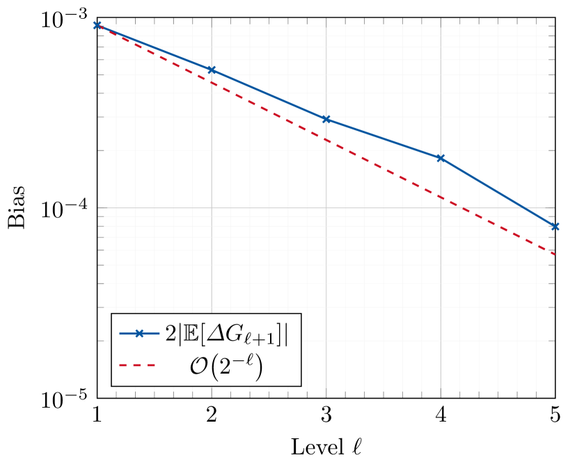
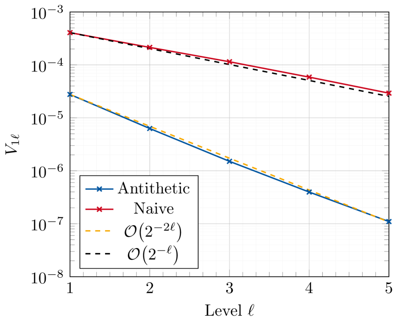
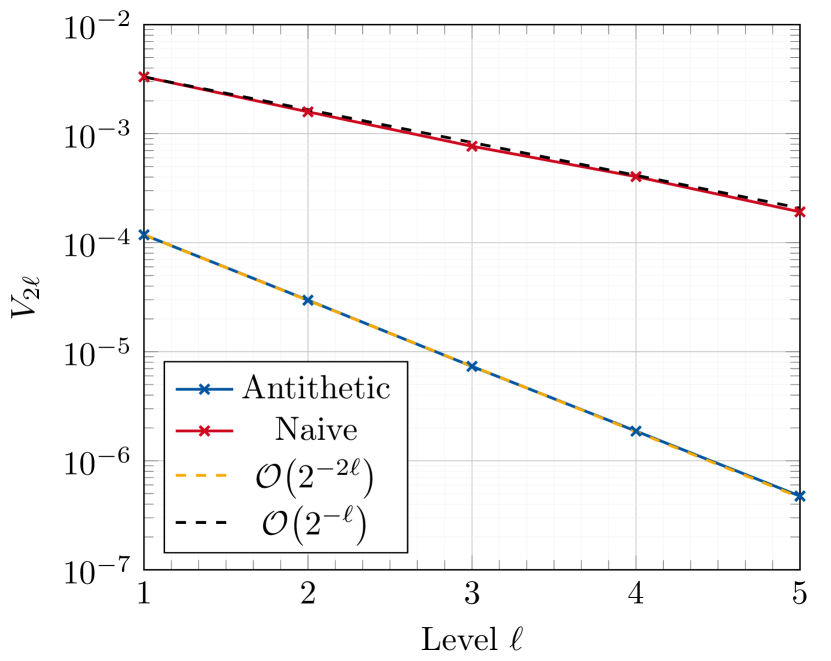
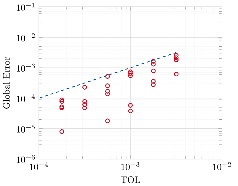
Figure 2 shows the results of Algorithm 2 in this setting to numerically verify complexity rates obtained from Theorem 1. We used $\bar{M}_{1}=10^{3}$,$\bar{M}_{2}=10^{2}$,$\tilde{M}_{1}=50$,$\tilde{M}_{2}=10^{3}$. To reduce work overload, we first used $\hat{M}_{1}=10^{3}$,$\hat{M}_{2}=10^{2}$ for levels $\ell=1,2$ and then (45) for all subsequent levels.

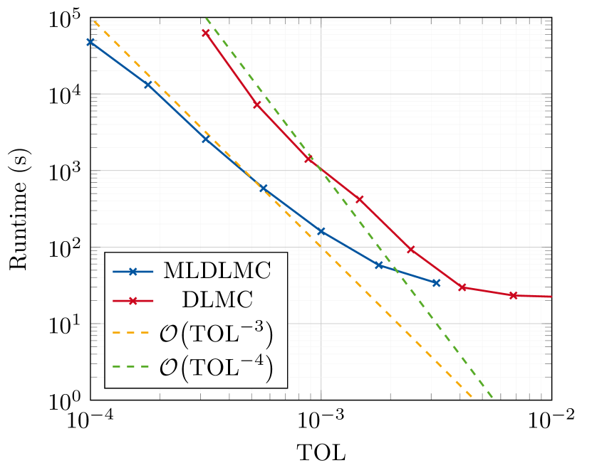
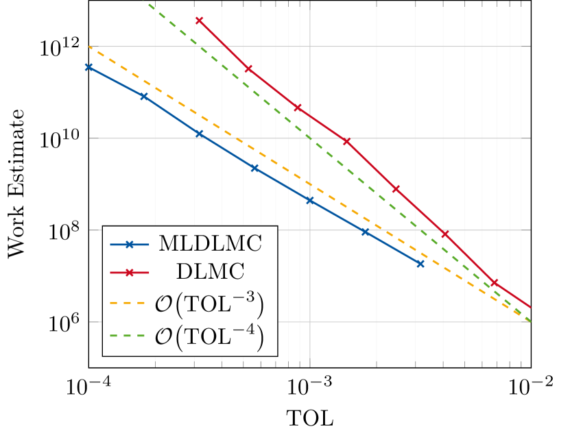
Figure 2(a) shows exact MLDLMC estimator error, estimated using a reference MLDLMC approximation with $\mathrm{TOL}=10^{-4}$, for separate Algorithm 2 runs for different prescribed error tolerances $\mathrm{TOL}$. The adaptive algorithm successfully satisfies the proposed MLDLMC estimator error constraints.

Figure 2(b) shows Algorithm 2 computational runtime for various error tolerances. The runtimes in Figure 2(b) include the cost of estimating the bias, $V_{1,\ell}$ and $V_{2,\ell}$. Runtimes for sufficiently small tolerances follow the predicted $\order{\mathrm{TOL}^{-3}}$ rate from Theorem 1.

Figure 2(c) shows estimated MLDLMC estimator computational work for various $\mathrm{TOL}$. Figures 2(b) and 2(c) clearly verify that the proposed MLDLMC estimator with antithetic sampler outperforms the single level DLMC estimator, achieving one order complexity reduction from $\order{\mathrm{TOL}^{-4}}$ to $\order{\mathrm{TOL}^{-3}}$.

(a) Global error with respect to tolerance $\mathrm{TOL}$

(b) Computational runtime with respect to tolerance $\mathrm{TOL}$

(c) Computational work estimate with respect to tolerance $\mathrm{TOL}$

Figure 2: Algorithm 2 applied to Kuramoto model for $G(x)=\cos{x}$.

5.2 Rare event objective function

We implemented the proposed MLDLMC algorithm with IS for the one-dimensional Kuramoto model with Lipschitz rare event observable $G(x)=\Psi(x-K)$ for large threshold $K\in\mathbb{R}$, where

$$\Psi(x)=\begin{cases}0&,\quad x<-0.5\\ 0.5+x&,\quad-0.5<x<0.5\\ 1&,\quad x>0.5\end{cases}\cdot$$ (47)

For the results shown, $K=2.5$ corresponds to expectation $\approx 3\times 10^{-3}$. We use the IS scheme introduced in Section 4.2 with IS control $\zeta$ obtained by solving (15) numerically using finite differences and linear interpolation throughout the domain. We first verify variance reduction in level difference estimators using $\zeta$ that minimizes single level estimator variance through two numerical experiments.

Experiment 1 investigated variance reduction on the conditional DLMC estimator of $\mathbb{E}\left[\Delta G_{\ell}\mid\mu^{\bar{P}|\bar{N}}\right]$. To generate Figure 3(a), $\mu^{\bar{P}|\bar{N}}$ was obtained with $\bar{P}=200$ particles and $\bar{N}=100$ time-steps. We used this law to both obtain IS control $\zeta$ and as an input to all decoupled MV-SDE realizations, and used Algorithm 1 for $\ell=3$ to estimate $\mathbb{E}\left[\Delta G_{\ell}\mid\mu^{\bar{P}|\bar{N}}\right]$.

Figure 3(a) compares sample means and squared coefficients of variation for the DLMC estimator with and without IS with respect to the number of sample paths $M$. Results verify that $\mathbb{E}\left[\Delta G_{\ell}\mid\mu^{\bar{P}|\bar{N}}\right]$ estimates with and without IS converge to the same value, whereas the squared coefficient of variation reduces approximately 100 fold with IS.

In experiment 2, we verify variance reduction for the DLMC estimator for $\mathbb{E}\left[\Delta G_{\ell}\right]$ with IS. To generate Figure 3(b), we used $\bar{P}=1000$ particles and $\bar{N}=100$ time steps to obtain $\mu^{\bar{P}|\bar{N}}$ to define IS control $\zeta$, and Algorithm 1 with $\ell=3$, $M_{1}=10^{3}$. The results verify estimator convergence with and without IS with significantly reduced squared coefficient of variation (approximately one order of magnitude) with IS.

(a) DLMC estimator for $\mathbb{E}\left[\Delta G_{3}\mid\mu^{\bar{P}|\bar{N}}\right]$ with and without IS (Left) sample mean; and (Right) squared coefficient of variation, with respect to number of sample paths $M$

(b) DLMC estimator for $\mathbb{E}\left[\Delta G_{3}\right]$ with and without IS (Left) sample mean; and (Right) squared coefficient of variation, with respect to number of sample paths in inner loop $M_{2}$.

Figure 3: Variance reduction in DLMC estimator for level differences using IS on Kuramoto model for $G(x)=\Psi(x-K)$

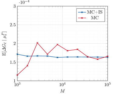
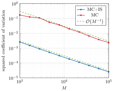
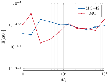
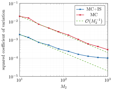
Figure 4 numerically corroborates Assumptions 1 and 2 to determine constants $\tilde{\alpha}$, $\tilde{w}$, and $\tilde{s}$ for the Kuramoto model with $G(x)=\Psi(x-K)$. The results verify Assumptions 1 and 2 with $\tilde{\alpha}=1$ and $\{\tilde{w},\tilde{s}\}=\{2,1\}$ for the antithetic sampler in (25). These rates imply $\order{\mathrm{TOL}^{-3}}$ complexity of the proposed MLDLMC estimator with IS.

(a) Assumption 1 for $G(x)=\Psi(x-K)$: DLMC bias estimator using Algorithm 1 with inputs $M_{1}=10^{2}$ and $M_{2}=10^{4}$ with respect to $\ell$

(b) Assumption 2 for $G(x)=\Psi(x-K)$: DLMC estimator for $V_{1,\ell}$ using Algorithm 3 with inputs $M_{1}=10^{2}$ and $M_{2}=10^{4}$ with respect to $\ell$

(c) Assumption 2 for $G(x)=\Psi(x-K)$: DLMC estimator for $V_{2,\ell}$ using Algorithm 3 with inputs $M_{1}=10^{2}$ and $M_{2}=10^{4}$ with respect to $\ell$.

Figure 4: Convergence rates of level differences using antithetic estimator for Kuramoto model with $G(x)=\Psi(x-K)$

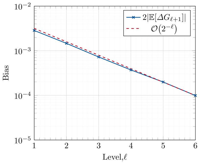
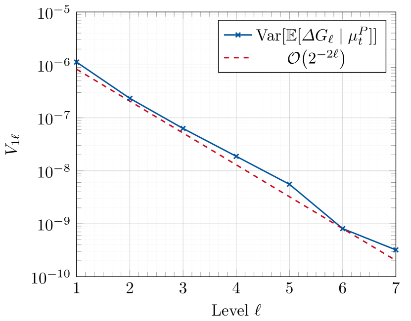
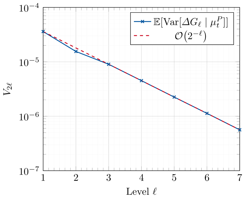
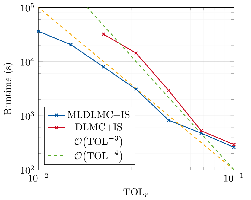
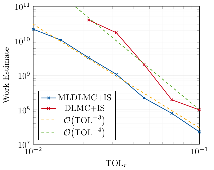
Figure 5 shows the results of Algorithm 2 in this setting and numerically verifies complexity rates obtained in Theorem 1. We used $\bar{P}=1000$ particles and $\bar{N}=100$ time steps to estimate $\mu^{\bar{P}|\bar{N}}$ to obtain IS control $\zeta$. We used $\bar{M}_{1}=10^{3}$,$\bar{M}_{2}=10^{2}$,$\tilde{M}_{1}=50$,$\tilde{M}_{2}=10^{3}$. To reduce work overload, we first used $\hat{M}_{1}=10^{3}$,$\hat{M}_{2}=10^{2}$ for levels $\ell=1,2$ and then (45) for all subsequent levels.

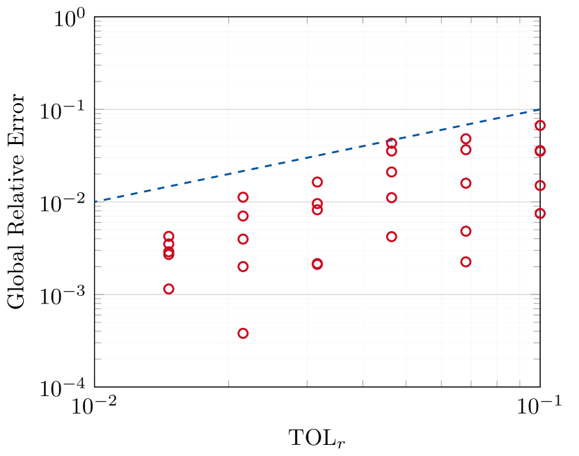
We observe that $K=2.5$ corresponds to an expected value $\approx 3.2\times 10^{-3}$. Figure 5(a) shows exact error for the proposed MLDLMC estimator, estimated using a reference MLDLMC approximation with $\mathrm{TOL}_{r}=1\%$, for multiple Algorithm 2 runs with various prescribed relative error tolerances.

The runtimes in Figure 5(b) includes estimation time of the bias, $V_{1,\ell}$ and $V_{2,\ell}$. Figure 5(b) confirms that computational runtime closely follows the predicted theoretical rate $\order{\mathrm{TOL}_{r}^{-3}}$ for small relative tolerances. Figure 5(c) shows computational work estimate for the MLDLMC estimator over prescribed $\mathrm{TOL}_{r}$ values. Figures 5(b) and 5(c) both show $\order{\mathrm{TOL}_{r}^{-3}}$ complexity for the MLDLMC estimator with IS and antithetic sampler, achieving one order complexity reduction compared with the single level DLMC estimator with the same IS scheme.

(a) Global error with respect to relative tolerance $\mathrm{TOL}_{r}$

(b) Computational runtime with respect to relative tolerance $\mathrm{TOL}_{r}$

(c) Computational work estimate with respect to relative tolerance $\mathrm{TOL}_{r}$

Figure 5: Algorithm 2 applied to Kuramoto model for $G(x)=\Psi(x-K)$ with $K=2.5$

6 Conclusion

This paper has shown both theoretically and numerically under certain assumptions, which could be verified numerically, the improvement of MLDLMC compared with single level DLMC estimator when used to approximate rare event quantities of interest that can be expressed as an expectation of some Lipschitz observable of the solution to stochastic particle systems in the mean field limit. We used the single level IS scheme introduced in our other work (Ben Rached et al., 2022) for all level difference estimators in the proposed MLDLMC estimator and verified substantial variance reduction numerically. The proposed novel MLDLMC estimator achieved $\order{\mathrm{TOL}_{r}^{-3}}$ complexity for the treated example; one order less than the single level DLMC estimator for prescribed relative error tolerance $\mathrm{TOL}_{r}$. Integrating the IS scheme ensured the associated constant also reduced significantly compared with the MLMC estimator for smooth, non-rare observables introduced in (Haji-Ali and Tempone, 2018).

Future study should include extending the IS scheme to higher-dimensional problems, using model reduction techniques or stochastic gradient based learning methods to solve the associated higher-dimensional stochastic optimal control problems. The IS scheme could be further improved by solving an optimal control problem that minimizes level difference estimator variance rather than the single level DLMC estimator. The MLDLMC algorithm could be optimized with respect to finding optimal parameters $\tau$ and $\theta$ (Haji-Ali et al., 2016b) or integrating a continuation MLMC algorithm (Collier et al., 2014). The present analysis could be extended to numerically handle non-Lipschitz rare event observables, such as the indicator function to compute rare event probabilities. Multiple discretization parameters for the decoupled MV-SDE ($P,N_{1},N_{2}$) suggest extending the current work to a multi-index Monte Carlo (Haji-Ali et al., 2016a; Haji-Ali and Tempone, 2018) setting to further reduce complexity.

Appendix A Proof for Theorem 1

For given level $L\in\mathbb{N}$, (37) provides the optimal number of samples to satisfy the variance constraint (29) for the proposed MLDLMC estimator. We bound the MLDLMC estimator (23) work as

$$\text{Work}[\mathcal{A}_{\textrm{MLMC}}] \lesssim\sum_{\ell=0}^{L}\left({M_{1,\ell}}P_{\ell}^{1+\gamma_{p}}N_{\ell}^{\gamma_{n}}+{M_{1,\ell}M_{2,\ell}}P_{\ell}^{\gamma_{p}}N_{\ell}^{\gamma_{n}}\right)$$

$$\lesssim\sum_{\ell=0}^{L}\left({(\mathcal{M}_{1,\ell}+1)}P_{\ell}^{1+\gamma_{p}}N_{\ell}^{\gamma_{n}}+{(\mathcal{M}_{1,\ell}+1)\left(\frac{\tilde{\mathcal{M}}_{\ell}}{\lceil\mathcal{M}_{1,\ell}\rceil}+1\right)}P_{\ell}^{\gamma_{p}}N_{\ell}^{\gamma_{n}}\right)$$

$$\leq\underbrace{\sum_{\ell=0}^{L}\left(\mathcal{M}_{1,\ell}P_{\ell}^{1+\gamma_{p}}N_{\ell}^{\gamma_{n}}+\tilde{\mathcal{M}}_{\ell}P_{\ell}^{\gamma_{p}}N_{\ell}^{\gamma_{n}}\right)}_{=W_{1},\text{objective function of \eqref{eqn:mldlmc_optim}}}$$

$$+\underbrace{\sum_{\ell=0}^{L}\left(P_{\ell}^{1+\gamma_{p}}N_{\ell}^{\gamma_{n}}+P_{\ell}^{\gamma_{p}}N_{\ell}^{\gamma_{n}}\right)}_{W_{2},\text{cost of one realization per level}}+\underbrace{{\sum_{\ell=0}^{L}\mathcal{M}_{1,\ell}P_{\ell}^{\gamma_{p}}N_{\ell}^{\gamma_{n}}}}_{=W_{3}}+\underbrace{{\sum_{\ell=0}^{L}\frac{\tilde{\mathcal{M}}_{\ell}}{\lceil\mathcal{M}_{1,\ell}\rceil}P_{\ell}^{\gamma_{p}}N_{\ell}^{\gamma_{n}}}}_{=W_{4}}\cdot$$ (48)

Since $P_{\ell}>1$ and $\gamma_{p}>0$, $W_{3}$ is always dominated by the first term in $W_{1}$, i.e. $\sum_{\ell=0}^{L}\mathcal{M}_{1,\ell}P_{\ell}^{1+\gamma_{p}}N_{\ell}^{\gamma_{n}}$. We now analyze each term individually.

Substituting (36) in $W_{1}$,

$$W_{1}=\frac{C_{\nu}^{2}}{(1-\theta)^{2}\mathrm{TOL}^{2}}\left(\sum_{\ell=0}^{L}\sqrt{P_{\ell}^{\gamma_{p}}N_{\ell}^{\gamma_{n}}}(\sqrt{V_{1,\ell}P_{\ell}}+\sqrt{V_{2,\ell}})\right)^{2}\cdot$$ (49)

Selecting level $L$ that satisfies (27) and using Assumption 1,

$$\absolutevalue{\mathbb{E}[G-G_{L}]}\leq C_{b}\tau^{-\tilde{\alpha}L}\approx\theta\mathrm{TOL}\cdot$$ (50)

and hence,

$$L=\left\lceil\frac{1}{\tilde{\alpha}}\log(\frac{C_{b}}{\theta}\mathrm{TOL}^{-1})\right\rceil\cdot$$ (51)

Using the hierarchies (21) and Assumption 2 in (48),

$$W_{1}\lesssim{\mathrm{TOL}^{-2}\left(\sum_{\ell=0}^{L}\tau^{\frac{1+\gamma_{p}+\gamma_{n}-\tilde{w}}{2}\ell}+\tau^{\frac{\gamma_{p}+\gamma_{n}-\tilde{s}}{2}\ell}\right)^{2}}\cdot$$ (52)

Since there are two terms in the summation in (52), we have two different cases as follows.

• Case 1: $\tilde{s}+1\geq\tilde{w}$, i.e., the first term dominates. $W_{1}$ can be expressed as

  $$W_{1}\lesssim{\mathrm{TOL}^{-2}\left(\sum_{\ell=0}^{L}\tau^{\frac{1+\gamma_{p}+\gamma_{n}-\tilde{w}}{2}\ell}\right)^{2}},$$ (53)

  and simplified using (51) and the sum of a geometric series,

  $$W_{1}\lesssim\begin{cases}{\mathrm{TOL}^{-2}}&\quad,{\tilde{w}>1+\gamma_{p}+\gamma_{n}}\\ {\mathrm{TOL}^{-2}(\log\mathrm{TOL}^{-1})^{2}}&\quad,{\tilde{w}=1+\gamma_{p}+\gamma_{n}}\\ {\mathrm{TOL}^{-2-\left(\frac{1+\gamma_{p}+\gamma_{n}-\tilde{w}}{\tilde{\alpha}}\right)}}&\quad,{\tilde{w}<1+\gamma_{p}+\gamma_{n}}\end{cases},$$ (54)

  which can be expressed more compactly as

  $$W_{1}\lesssim{\mathrm{TOL}^{-2-\max\left(0,\frac{1+\gamma_{p}+\gamma_{n}-\tilde{w}}{\tilde{\alpha}}\right)}(\log\mathrm{TOL}^{-1})^{2\crossproduct\mathbbm{1}_{\{\tilde{w}=1+\gamma_{p}+\gamma_{n}\}}}}\cdot$$ (55)

• Case 2: $\tilde{s}+1<\tilde{w}$, i.e., the second term dominates. Express $W_{1}$ as

  $$W_{1}\lesssim{\mathrm{TOL}^{-2}\left(\sum_{\ell=0}^{L}\beta^{\frac{\gamma_{p}+\gamma_{n}-\tilde{s}}{2}\ell}\right)^{2}},$$ (56)

  and simplify using the sum of a geometric series,

  $$W_{1}\lesssim\begin{cases}{\mathrm{TOL}^{-2}}&\quad,{\tilde{s}>\gamma_{p}+\gamma_{n}}\\ {\mathrm{TOL}^{-2}(\log\mathrm{TOL}^{-1})^{2}}&\quad,{\tilde{s}=\gamma_{p}+\gamma_{n}}\\ {\mathrm{TOL}^{-2-\left(\frac{\gamma_{p}+\gamma_{n}-\tilde{s}}{\tilde{\alpha}}\right)}}&\quad,{\tilde{s}<\gamma_{p}+\gamma_{n}}\end{cases},$$ (57)

  which can be expressed more compactly as

  $$W_{1}\lesssim{\mathrm{TOL}^{-2-\max\left(0,\frac{\gamma_{p}+\gamma_{n}-\tilde{s}}{\tilde{\alpha}}\right)}(\log\mathrm{TOL}^{-1})^{2\crossproduct\mathbbm{1}_{\{\tilde{s}=\gamma_{p}+\gamma_{n}\}}}}\cdot$$ (58)

  In this case also, $W_{1}$ is of higher order than $W_{3}$ since we know that $W_{3}$ is of lower order than the first term in $W_{1}$. Hence, $W_{3}$ is always of lower order than $W_{1}$.

Using (21), we get for $W_{2}$,

$$W_{2} \lesssim{\mathrm{TOL}^{-\left(\frac{1+\gamma_{p}+\gamma_{n}}{\tilde{\alpha}}\right)}}\cdot$$ (59)

Next, we look at $W_{4}$.

$$W_{4} =\sum_{\ell=0}^{L}\frac{\tilde{\mathcal{M}}_{\ell}}{\lceil\mathcal{M}_{1,\ell}\rceil}P_{\ell}^{\gamma_{p}}N_{\ell}^{\gamma_{n}}$$

$$\leq\sum_{\ell=0}^{L}\frac{\tilde{\mathcal{M}}_{\ell}}{\max\{1,\mathcal{M}_{1,\ell}\}}P_{\ell}^{\gamma_{p}}N_{\ell}^{\gamma_{n}}$$

$$=\sum_{\ell=0}^{L}\min\{\tilde{\mathcal{M}}_{\ell}P_{\ell}^{\gamma_{p}}N_{\ell}^{\gamma_{n}},\frac{\tilde{\mathcal{M}}_{\ell}}{\mathcal{M}_{1,\ell}}P_{\ell}^{\gamma_{p}}N_{\ell}^{\gamma_{n}}\}$$

$$\leq\sum_{\ell=0}^{L}\tilde{\mathcal{M}}_{\ell}P_{\ell}^{\gamma_{p}}N_{\ell}^{\gamma_{n}}\cdot$$ (60)

This is of the same order or less than that of $W_{1}$. Now we still need to ensure the complexity order of $W_{1}$ is greater than that of $W_{2}$ for the proposed MLDLMC method to be feasible. Comparing (59) to $W_{1}$ for the different cases, the following condition ensures $W_{1}$ is the dominant term

$$\tilde{\alpha}\geq\frac{1}{2}\min(\tilde{w},1+\tilde{s},1+\gamma_{p}+\gamma_{n})\cdot$$ (61)

Thus, (61) along with (55), (58) complete the proof.

Appendix B Estimating $V_{1,\ell},V_{2,\ell}$ for adaptive MLDLMC

Inputs: $\ell,M_{1},M_{2},\zeta(\cdot,\cdot)$;

for $m_{1}=1,\ldots,M_{1}$ do

       Generate $\mu_{\ell}(\omega_{1:P_{\ell}}^{(\ell,m_{1})})$ using (17);

       for $a=1,\ldots,\tau$ do

             Generate $\mu_{\ell-1}^{(a)}(\omega_{(a-1)P_{\ell-1}+1:aP_{\ell-1}}^{(\ell,m_{1})})$ using (17);

       end for

      for $m_{2}=1,\ldots,M_{2}$ do

             Given $\mu_{\ell}(\omega_{1:P_{\ell}}^{(\ell,m_{1})})$ and $\zeta(\cdot,\cdot)$, generate sample path of (8) at level $\ell$ with $\tilde{\omega}^{(\ell,m_{2})}$;

             Compute $G_{\ell}^{IS}(\omega_{1:P_{\ell}}^{(\ell,m_{1})},\tilde{\omega}^{(\ell,m_{2})})$;

             for $a=1,\ldots,\tau$ do

                   Given $\mu_{\ell-1}^{(a)}(\omega_{(a-1)P_{\ell-1}+1:aP_{\ell-1}}^{(\ell,m_{1})})$ and $\zeta(\cdot,\cdot)$, generate sample path of $\eqref{eqn:decoupled_mvsde}$ at level $\ell-1$ with $\tilde{\omega}^{(\ell,m_{2})}$;

                   Compute $G_{\ell-1}^{IS}(\omega_{(a-1)P_{\ell-1}+1:aP_{\ell-1}}^{(\ell,m_{1})},\tilde{\omega}^{(\ell,m_{2})})$;

                  

             end for

            $\hat{\mathcal{G}}_{\ell-1}^{IS}(\omega_{1:P_{\ell}}^{(\ell,m_{1})},\tilde{\omega}^{(\ell,m_{2})})=\frac{1}{\tau}\sum_{a=1}^{\tau}G_{\ell-1}^{IS}(\omega_{(a-1)P_{\ell-1}+1:aP_{\ell-1}}^{(\ell,m_{1})},\tilde{\omega}^{(\ell,m_{2})})$;

            

       end for

      $\Delta G_{\ell}^{(m_{1},m_{2})}=(G_{\ell}^{IS}-\hat{\mathcal{G}}_{\ell-1}^{IS})(\omega_{1:P_{\ell}}^{(\ell,m_{1})},\tilde{\omega}^{(\ell,m_{2})})$;

       Approximate $\mathbb{E}\left[\Delta G_{\ell}\mid\{\mu_{\ell},\mu_{\ell-1}\}(\omega_{1:P_{\ell}}^{(\ell,m_{1})})\right]$ by $\frac{1}{M_{2}}\sum_{m_{2}=1}^{M_{2}}\Delta G_{\ell}^{(m_{1},m_{2})}$;

       Approximate $\mathrm{Var}\left[\Delta G_{\ell}\mid\{\mu_{\ell},\mu_{\ell-1}\}(\omega_{1:P_{\ell}}^{(\ell,m_{1})})\right]$ by sample variance of $\left\{\Delta G_{\ell}^{(m_{1},m_{2})}\right\}_{m_{2}=1}^{M_{2}}$ ;

      

end for

Approximate $V_{1,\ell}$ by sample variance of $\left\{\mathbb{E}\left[\Delta G_{\ell}\mid\{\mu_{\ell},\mu_{\ell-1}\}(\omega_{1:P_{\ell}}^{(\ell,m_{1})})\right]\right\}_{m_{1}=1}^{M_{1}}$;

Approximate $V_{2,\ell}$ by $\frac{1}{M_{1}}\sum_{m_{1}=1}^{M_{1}}\mathrm{Var}\left[\Delta G_{\ell}\mid\{\mu_{\ell},\mu_{\ell-1}\}(\omega_{1:P_{\ell}}^{(\ell,m_{1})})\right]$.

Algorithm 3 Estimating $V_{1,\ell}$ and $V_{2,\ell}$ for adaptive MLDLMC

References

- Acebron et al. (2005) J.A Acebron, L.L. Bonilla, J.P Vicente, F. Ritort, and R. Spigler. The Kuramoto model: A simple paradigm for synchronization phenomena. Reviews of Modern Physics, 77(1):137–185, 2005. doi: https://doi.org/10.1103/RevModPhys.77.137.
- Ash and Doléans-Dade (2000) R.B. Ash and C. Doléans-Dade. Probability and Measure Theory, volume 23. Harcourt/Academic Press, San Diego, 2000.
- Ben Alaya et al. (2022) M. Ben Alaya, K. Hajji, and A. Kebaier. Adaptive importance sampling for multilevel Monte Carlo Euler method. Stochastics, pages 1–25, 2022. doi: https://doi.org/10.1080/17442508.2022.2084338.
- Ben Amar et al. (2022) E. Ben Amar, N Ben Rached, A.L. Haji-Ali, and R. Tempone. Efficient importance sampling algorithm applied to the performance analysis of wireless communication systems estimation. arXiv Preprint:2201.01340, 2022. doi: https://doi.org/10.48550/arxiv.2201.01340.
- Ben Hammouda et al. (2021) C. Ben Hammouda, N. Ben Rached, R. Tempone, and S. Wiechert. Efficient importance sampling via stochastic optimal control for stochastic reaction networks. arXiv Preprint:2110.14335, 2021. doi: https://doi.org/10.48550/arxiv.2110.14335.
- Ben Hammounda et al. (2020) C. Ben Hammounda, N. Ben Rached, and R. Tempone. Importance sampling for a robust and efficient multilevel Monte Carlo estimator for stochastic reaction netowrks. Statistics and Computing, 30:1665–1689, 2020. doi: https://doi.org/10.1007/s11222-020-09965-3.
- Ben Rached et al. (2022) N. Ben Rached, A.L. Haji-Ali, S.M. Subbiah Pillai, and R. Tempone. Single level importance sampling for McKean-Vlasov stochastic differential equation. arXiv Preprint:2207.06926, 2022. doi: https://doi.org/10.48550/arxiv.2207.06926.
- Bossy and Talay (1996) M. Bossy and D. Talay. Convergence rate for the approximation of the limit law of weakly interacting particles: application to the Burgers equation. Annals of Applied Probability, 6(3):818–861, 1996. doi: https://doi.org/10.1214/aoap/1034968229.
- Bossy and Talay (1997) M. Bossy and D. Talay. A stochastic particle method for the McKean-Vlasov and the Burgers equation. Mathematics of Computation, 66(217):157–192, 1997. URL http://www-sop.inria.fr/members/Denis.Talay/fichiers-pdf/bossy-talay-mathcomp.pdf.
- Buckdahn et al. (2017) R. Buckdahn, J. Li, S. Peng, and C. Rainer. Mean-field stochastic differential equations and associated PDEs. The Annals of Probability, 45(2):824–878, 2017. doi: https://doi.org/10.1214/15-AOP1076.
- Bujok et al. (2015) K. Bujok, B.M. Hambly, and C. Reisinger. Multilevel simulation of functionals of Bernoulli random variables with application to basket credit derivatives. Methodology and Computing in Applied Probability, 17(3):579–604, 2015. doi: https://doi.org/10.1007/s11009-013-9380-5.
- Bush et al. (2011) N. Bush, B.M. Hambly, H.Haworth, and L. Jin. Stochastic evolution equations in portfolio credit modelling. SIAM Journal of Financial Mathematics, 2(1):627–664, 2011. doi: http://dx.doi.org/10.1137/100796777.
- Collier et al. (2014) N. Collier, Haji-Ali.A.L., F. Nobile, E. von Schwerin, and R. Tempone. A continuation multilevel Monte Carlo algorithm. BIT Numerical Mathematics, 55(2):399–432, 2014. doi: https://doi.org/10.1007/s10543-014-0511-3.
- Crisan and McMurray (2018) D. Crisan and E. McMurray. Smoothing properties of McKean–Vlasov SDEs. Probability Theory and Related Fields, 171(1):97–148, 2018. doi: https://doi.org/10.1007/s00440-017-0774-0.
- Crisan and McMurray (2019) D. Crisan and E. McMurray. Cubature on Wiener space for McKean–Vlasov SDEs with smooth scalar interaction. The Annals of Applied Probability, 29(1):130–177, 2019.
- Crisan and Xiong (2010) D. Crisan and J. Xiong. Approximate McKean-Vlasov representations for a class of SPDEs. Stochastics, 82(1):53–68, 2010. doi: https://doi.org/10.1080/17442500902723575.
- Cumin and Unsworth (2007) D. Cumin and C.P. Unsworth. Generalising the Kuramoto model for the study of neuronal synchronisation in the brain. Physica D: Nonlinear Phenomena, 226(2):181–196, 2007. doi: https://doi.org/10.1016/j.physd.2006.12.004.
- Dobramysl et al. (2016) U. Dobramysl, S. Rudiger, and R. Erban. Particle-based multiscale modeling of calcium puff dynamics. Multiscale Modeling and Simulation, 14(3):997–1016, 2016. doi: https://doi.org/10.1137/15M1015030.
- dos Reis et al. (2018) G. dos Reis, G. Smith, and P. Tankov. Importance sampling for McKean-Vlasov SDEs. arXiv Preprint:1803.09320, 2018. doi: https://doi.org/10.48550/arxiv.1803.09320.
- dos Reis et al. (2022) G. dos Reis, S. Engelhardt, and G. Smith. Simulation of McKean–Vlasov SDEs with super-linear growth. IMA Journal of Numerical Analysis, 42(1):874–922, 2022. doi: https://doi.org/10.1093/imanum/draa099.
- Dupuis and Wang (2004) P. Dupuis and H. Wang. Importance sampling, large deviations, and differential games. Stochastics: An International Journal of Probability and Stochastic Processes, 76(6):481–508, 2004. doi: https://doi.org/10.1080/10451120410001733845.
- Erban and Haskovec (2012) R. Erban and J. Haskovec. From individual to collective behaviour of coupled velocity jump processes: a locust example. Kinetic and Related Models, 5(4):817–842, 2012. doi: https://doi.org/10.3934/krm.2012.5.817.
- Fang and Giles (2019) W. Fang and M.B. Giles. Multilevel Monte Carlo method for ergodic SDEs without contractivity. Journal of Mathematical Analysis and Applications, 476:149–176, 2019. doi: https://doi.org/10.1016/j.jmaa.2018.12.032.
- Giles (2008) M.B. Giles. Multilevel Monte Carlo path simulation. Operations Research, 56(3):607–617, 2008. doi: https://doi.org/10.1287/opre.1070.0496.
- Giles (2015) M.B. Giles. Multilevel Monte Carlo methods. Acta Numerica, 24(1):259–328, 2015. doi: https://doi.org/10.1017/S096249291500001X.
- Giles and Szpruch (2014) M.B. Giles and L. Szpruch. Antithetic multilevel Monte Carlo estimation for multi-dimensional SDEs without Lévy area simulation. The Annals of Applied Probability, 24(4):1585–1620, 2014. doi: https://doi.org/10.1214/13-aap957.
- Haji-Ali (2012) A.L. Haji-Ali. Pedestrian flow in the mean field limit. KAUST Research Repository, 2012. doi: https://doi.org/10.25781/KAUST-N103E.
- Haji-Ali and Tempone (2018) A.L. Haji-Ali and R. Tempone. Multilevel and multi-index Monte Carlo methods for the McKean-Vlasov equation. Statistics and Computing, 28(4):923–935, 2018. doi: https://doi.org/10.1007/s11222-017-9771-5.
- Haji-Ali et al. (2016a) A.L. Haji-Ali, F. Nobile, and R. Tempone. Multi-index Monte Carlo: When sparsity meets sampling. Numerical Mathematics, 132(1):767–806, 2016a. doi: https://doi.org/10.1007/s00211-015-0734-5.
- Haji-Ali et al. (2016b) A.L. Haji-Ali, F. Nobile, E. von Schwerin, and R. Tempone. Optimization of mesh hierarchies in multilevel Monte Carlo samplers. Stochastics and Partial Differential Equations Analysis and Computations, 4:76–112, 2016b. doi: https://doi.org/10.1007/s40072-015-0049-7.
- Haji-Ali et al. (2021) A.L. Haji-Ali, H. Hoel, and R. Tempone. A simple approach to proving the existence, uniqueness, and strong and weak convergence rates for a broad class of McKean-Vlasov equations. arXiv Preprint:2101.00886, 2021. doi: https://doi.org/10.48550/arxiv.2101.00886.
- Hammersley et al. (2021) W. Hammersley, D. Siska, and L. Szpruch. Weak existence and uniqueness for McKean-Vlasov SDEs with common noise. The Annals of Probability, 49(2):527–555, 2021. doi: https://doi.org/10.1214/20-AOP1454.
- Hartmann et al. (2015) C. Hartmann, C. Schütte, and W. Zhang. Projection-based algorithms for optimal control and importance sampling of diffusions. 2015.
- Hartmann et al. (2016) C. Hartmann, C. Schütte, and W. Zhang. Model reduction algorithms for optimal control and importance sampling of diffusions. Nonlinearity, 29(8):2298 – 2326, 2016. doi: https://doi.org/10.1088/0951-7715/29/8/2298.
- Hartmann et al. (2017) C. Hartmann, L. Richter, C. Schütte, and W. Zhang. Variational characterization of free energy: Theory and algorithms. Entropy, 2017. doi: https://doi.org/10.3390/e19110626.
- Hartmann et al. (2018) C. Hartmann, C. Schütte, M. Weber, and W. Zhang. Importance sampling in path space for diffusion processes with slow-fast variables. Probability Theory and Related Fields, 170:177–228, 2018. doi: https://doi.org/10.1007/s00440-017-0755-3.
- Kebaier and Lelong (2018) A. Kebaier and J. Lelong. Coupling importance sampling and multilevel Monte Carlo using sample average approximation. Methodology and Computing in Applied Probability, 20:611–641, 2018. doi: https://doi.org/10.1007/s11009-017-9579-y.
- Kloeden and Platen (1992) P.E. Kloeden and E. Platen. Numerical Solution of Stochastic Differential Equations. Springer, Berlin, 1992. doi: https://doi.org/10.1007/978-3-662-12616-5.
- Kroese et al. (2013) D. Kroese, T. Taimre, and Z.I. Botev. Handbook of Monte Carlo Methods. Wiley, 2013.
- Lemaire and Pagés (2013) V. Lemaire and G. Pagés. Multilevel Richardson-Romberg extrapolation. arXiv Preprint:1401.1177, 2013. doi: https://doi.org/10.3150/2F16-bej822.
- Li et al. (2022) Y. Li, X. Mao, Q. Song, F. Wu, and G. Yin. Strong convergence of Euler-Maruyama schemes for McKean-Vlasov stochastic differential equations under local Lipschitz conditions of state variables. IMA Journal of Numerical Analysis, 2022. doi: https://doi.org/10.1093/imanum/drab107.
- McKean (1966) H.P. McKean. A class of Markov processes associated with nonlinear parabolic equations. Proceedings of the National Academy of Sciences of the United States of America, 56(6):1907–1911, 1966. doi: https://doi.org/10.1073/pnas.56.6.1907.
- Méléard (1996) S. Méléard. Asymptotic behaviour of some interacting particle systems; McKean-Vlasov and Boltzmann models. In D. Talay and L. Tubaro, editors, Probabilistic Models for Nonlinear Partial Differential Equations, volume 1627, pages 42–95. Springer, 1996. doi: https://doi.org/10.1007/BFb0093177.
- Mishura and Veretennikov (2016) Y.S. Mishura and A.Y. Veretennikov. Existence and uniqueness theorems for solutions of McKean–Vlasov stochastic equations. arXiv Preprint:1603.02212, 2016. doi: https://doi.org/10.48550/arxiv.1603.02212.
- Rosin et al. (2014) M.S. Rosin, L.F. Ricketson, A.M. Dimits, R.E. Caflisch, and B.I. Cohen. Multilevel Monte Carlo simulation of Coulomb collisions. Journal of Computational Physics, 274:140–157, 2014. doi: https://doi.org/10.1016/j.jcp.2014.05.030.
- Sivashinsky (1977) G.I. Sivashinsky. Diffusional-thermal theory of cellular flames. Combustion Science and Technology, 15(3-4):137–146, 1977. doi: https://doi.org/10.1080/00102207708946779.
- Sznitman (1991) A.S. Sznitman. Topics in propagation of chaos. Ecole d’Eté de Probabilités de Saint-Flour XIX — 1989, 1464:165–251, 1991. doi: https://doi.org/10.1007/BFb0085169.
- Szpruch and Tse (2019) L. Szpruch and A. Tse. Antithetic multilevel particle system sampling method for McKean-Vlasov SDEs. arXiv Preprint:1903.07063, 2019. doi: https://doi.org/10.1214/20-aap1614.
- Szpruch et al. (2019) L. Szpruch, S. Tan, and A. Tse. Iterative multilevel particle approximation for McKean–Vlasov SDEs. The Annals of Applied Probability, 29(4):2230–2265, 2019. doi: https://doi.org/10.1214/18-AAP1452.
- Zhang et al. (2014) W. Zhang, H. Wang, C. Hartmann, M. Weber, and C. Schütte. Applications of the cross-entropy method to importance sampling and optimal control of diffusions. SIAM Journal on Scientific Computing, 36:A2654–A2672, 01 2014. doi: http://dx.doi.org/10.1137/14096493X.