Giant oscillations of diffusion in ac-driven periodic systems

Abstract

We revisit the problem of diffusion in a driven system consisting of an inertial Brownian particle moving in a symmetric periodic potential and subjected to a symmetric time-periodic force. We reveal parameter domains in which diffusion is normal in the long time limit and exhibits intriguing giant damped quasiperiodic oscillations as a function of the external driving amplitude. As the mechanism behind this effect we identify the corresponding oscillations of difference in the number of locked and running trajectories which carries the leading contribution to the diffusion coefficient. Our findings can be verified experimentally in a multitude of physical systems including colloidal particles, Josephson junction or cold atoms dwelling in optical lattices, to name only a few.

Processes occurring at the micro and nano-world are strongly influenced by thermal fluctuations whose intensity is determined by temperature of the system. A typical example is Brownian motion of a classical particle with erratic and unpredictable trajectories that are commonly characterized by a diffusion coefficient which in equilibrium is proportional to temperature. Because the ac-driven systems are out of equilibrium there can exist certain domains of the system parameters in which unexpected behaviour is encountered. In this work, we study a paradigmatic model of diffusion phenomena in nonequilibrium statistical physics that for decades has been applied to classical systems. We identify parameter regimes in which diffusion is normal in the long time limit, however, its dependence on the system parameter exhibits intriguing giant damped quasi-periodic oscillations. Our findings can be corroborated experimentally in various systems including, among others, colloidal systems, Josephson junctions and cold atoms dwelling in optical lattices.

I Introduction

Processes and phenomena in systems far from equilibrium can exhibit unexpected and unusual properties. They are ubiquitous in Nature ranging from the microscale to the macroscale. We quote only a few simplest and popular examples intensively studied in physics: stochastic benzi1981 ; gammaitoni1998 or coherence pikovsky1997 ; lindner2004 resonance, ratchet effect hanggi2009 ; actrat2017 , absolute negative mobility machura2007 ; nagel2008 ; slapik2019 ; spiechowicz2019njp , anomalous transport and anomalous diffusion klages2008 ; metzler2014 ; marchenko2014 ; spiechowicz2016njp ; marchenko2017 ; spiechowicz2017chaos ; marchenko2018 ; marchenko2019 . Diffusion plays a key role in numerous processes in physics, chemistry, biology and engineering. Moreover, this concept is exploited in sociology, politics and culture as a measure of spread of ideas, values, concepts, knowledge, practices, behaviors, materials, symbols and so on socjology . For normal diffusion described by the Einstein relation for a Brownian particle, the diffusion coefficient $D$ depends only on two parameters: it monotonically increases with increasing temperature $T$ and decreases when the friction coefficient grows. However, under nonequilibrium conditions, the dependence of $D$ on the system parameters may be surprising and non-monotonic. There are many scenarios to move systems out of equilibrium. One of the simplest way is to apply a constant force. The next is to use a time periodic perturbation. Recently, the great interest has been attracted to active fluctuations marchetti2013 ; spiechowicz2014pre ; bechinger2016 which appear e.g. in living cells where energy is provided in the form of biochemical reactions that drives active cellular processes gnesotto2018 . In such systems diffusion can be normal, however even then it is usually non-Gaussian wang2012 ; metzler2017 ; bialas2020 or it simply is anomalous metzler2014 , i.e. exhibits subdiffusive or superdiffusive behaviour. In the paper, we consider the case when the applied time periodic force continually supplies energy to the system and drives it far from thermodynamic equilibrium. We study diffusion and its dependence on the amplitude of this external driving. We find parameter regimes where the diffusion coefficient exhibits intriguing giant damped quasi-periodic oscillations.

The paper is organized as follows. In Sec. II, we formulated the model in terms of the Langevin equation. In Sec. III, we define quantifiers used to characterize the diffusion process. Sec. IV contains a description of simulations. In Sec. V we present the main result of the paper, i.e. the dependence of the diffusion coefficient on the amplitude of the ac-driving and explain its origin. The last section provides summary.

II Description of the model

We study a relatively simple model of a system in a nonequilibrium state. It is a classical Brownian particle of mass $M$ subjected to a one-dimensional, spatially periodic potential $U(x)$ and driven by an unbiased and symmetric time-periodic force $F(t)$. Its dynamics can be described by the Langevin equation in the form spiechowicz2016njp

$$M\ddot{x}+\Gamma\dot{x}=-U^{\prime}(x)+F(t)+\sqrt{2\Gamma k_{B}T}\,\xi(t),$$ (1)

where the dot and the prime denotes differentiation with respect to time $t$ and the particle coordinate $x$, respectively. The parameter $\Gamma$ is the friction coefficient. The potential $U(x)$ is assumed to be symmetric of spatial period $L$ and the barrier height $2\Delta U$ reading

$$U(x)=U(x+L)=-\Delta U\cos{\left(\frac{2\pi}{L}x\right)}.$$ (2)

The external ac-driving force of amplitude $A$ and angular frequency $\Omega$ has the simplest harmonic form

$$F(t)=A\sin{(\Omega t)}.$$ (3)

Thermal equilibrium fluctuations due to interaction of the particle with its environment of temperature $T$ are modelled as $\delta$-correlated Gaussian white noise of zero-mean value,

$$\langle\xi(t)\rangle=0,\quad\langle\xi(t)\xi(s)\rangle=\delta(t-s),$$ (4)

where the bracket $\langle\cdot\rangle$ denotes an average over white noise realizations (ensemble average). The noise intensity $2\Gamma k_{B}T$ in Eq. (1) follows from the fluctuation-dissipation theorem kubo1966 , where $k_{B}$ is the Boltzmann constant. If $A=0$ the stationary state is a thermal equilibrium state. If $A\neq 0$, then the external force $F(t)$ drives the system away from the equilibrium state.

There are several physical systems risken that can be modelled by Eq. (1). One can mention the semiclassical dynamics of the phase difference across a Josephson junction and its variations including e.g. the SQUIDs kautz1996 ; spiechowicz2015chaos ; blackburn2016 as well as the dynamics of cold atoms dwelling in optical lattices denisov2014 ; lutz2013 ; kindermann2017 .

The model given by Eq. (1) has been studied for decades and used for analysis of various noisy phenomena in both deterministic regular and chaotic regimes. We refer the interested reader to the review paper kautz1996 and references therein. Yet, there still remain new phenomena to be uncovered for this system, which in turn carry the potential for new applications. As recent examples we can quote a non-monotonic temperature dependence of a diffusion coefficient in normal diffusion regimes spiechowicz2016njp ; spiechowicz2017chaos ; marchenko2018 and transient, yet extended time-dependent anomalous diffusion spiechowicz2016scirep ; spiechowicz2017scirep ; spiechowicz2019chaos , to name but a few.

Now, we transform Eq. (1) to its dimensionless form. To this aim we use the following scales as characteristic units of length and time

$$\hat{x}=2\pi\frac{x}{L},\quad\hat{t}=\frac{t}{\tau_{0}},\quad\tau_{0}=\frac{L}{2\pi}\sqrt{\frac{M}{\Delta U}}.$$ (5)

Under such a procedure Eq. (1) assumes the form

$$\ddot{\hat{x}}+\gamma\dot{\hat{x}}=-\sin{\hat{x}}+a\sin(\omega\hat{t})+\sqrt{2\gamma Q}\hat{\xi}(\hat{t}).$$ (6)

In this scaling the dimensionless mass $m=1$ and the remaining four dimensionless parameters read

$$\gamma=\frac{\tau_{0}}{\tau_{1}},\quad a=\frac{1}{2\pi}\frac{L}{\Delta U}A,\quad\omega=\tau_{0}\Omega,\quad Q=\frac{k_{B}T}{\Delta U},$$ (7)

where the second characteristic time is $\tau_{1}=M/\Gamma$. It has the physical interpretation of the relaxation time for the velocity of the free Brownian particle. On the other hand, the characteristic time $\tau_{0}$ is related to the period of small oscillations inside the potential $U(x)$ wells.

The rescaled potential of the period $L=2\pi$ is $\hat{U}(\hat{x})=U((L/2\pi)\hat{x})/\Delta U=-\cos{\hat{x}}$ and the corresponding potential force is $-\hat{U}^{\prime}(\hat{x})=-\sin\hat{x}$. The rescaled thermal noise is $\hat{\xi}(\hat{t})=(L/2\pi\Delta U)\xi(t)=(L/2\pi\Delta U)\xi(\tau_{0}\hat{t})$ and has the same statistical properties as $\xi(t)$; i.e., $\langle\hat{\xi}(\hat{t})\rangle=0$ and $\langle\hat{\xi}(\hat{t})\hat{\xi}(\hat{s})\rangle=\delta(\hat{t}-\hat{s})$. The dimensionless noise intensity $Q$ is the ratio of thermal energy and half of the activation energy the particle needs to overcome the nonrescaled potential barrier. From now on we shall stick to these dimensionless variables. In order to simplify the notation further we omit the hat-notation in Eq. (6).

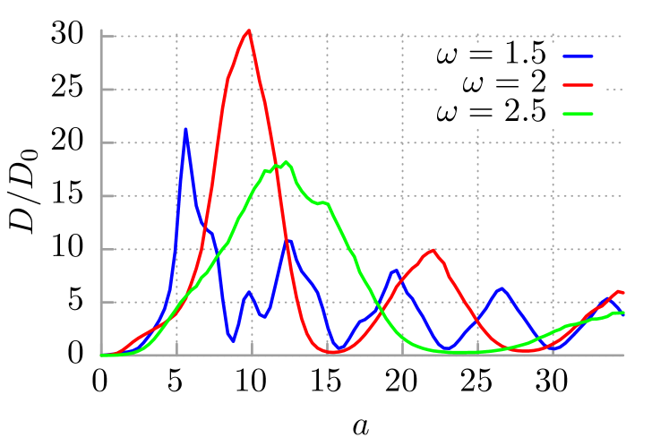
Figure 1: The rescaled diffusion coefficient $D/D_{0}$, where $D_{0}=Q/\gamma$ is free thermal diffusion, as a function of the amplitude $a$ of the ac-driving for selected values of its frequency $\omega$. Other parameters are: $\gamma=0.03$ and temperature $Q=0.5$

III Quantifiers used for analysis of diffusion

Diffusion is characterized by the mean square deviation (variance) of the particle position $x(t)$, namely,

$$\langle\Delta x^{2}(t)\rangle=\langle\left[x(t)-\langle x(t)\rangle\right]^{2}\rangle=\langle x^{2}(t)\rangle-\langle x(t)\rangle^{2}.$$ (8)

Here and below $\langle\cdot\rangle$ stands for the average over thermal noise realizations as well as over initial coordinates $x(0)$ and velocities $v(0)=\dot{x}(0)$ of the Brownian particle. For normal diffusion regime $\langle\Delta x^{2}(t)\rangle$ is a linear function of time and the diffusion coefficient can be defined by the relation spiechowicz2016scirep

$$D=\lim_{t\to\infty}\frac{\langle\Delta x^{2}(t)\rangle}{2t}.$$ (9)

As we will demonstrate the spread of position trajectories measured by the diffusion coefficient can be determined by behavior of the particle velocity. A relevant quantity characterizing transport of the Brownian particle is time averaged velocity

$$\overline{v}=\lim_{t\to\infty}\frac{1}{t}\int_{0}^{t}ds\,\dot{x}(s).$$ (10)

Since the system given by Eq. (6) is symmetric and unbiased a preferential direction of motion is forbidden in the long time limit. Consequently, the ensemble and time averaged velocity must vanish for both zero and non-zero temperature regimes denisov2014

$$\langle\overline{v}\rangle\equiv 0.$$ (11)

The latter is mandatory for the deterministic variant of dynamics which may be non-ergodic and therefore sensitive to the specific choice of starting position and velocity of the particle spiechowicz2016scirep . However, for any non-zero temperature $Q>0$ the system is ergodic and initial conditions do not affect properties of the system in the long time stationary regime. Due to the above condition the spread of time averaged velocity can be quantified solely by its second moment, i.e.

$$\sigma_{\overline{v}}^{2}=\langle\overline{v}^{2}\rangle-\langle\overline{v}\rangle^{2}\equiv\langle\overline{v}^{2}\rangle.$$ (12)

Figure 2: The rescaled diffusion coefficient $D/D_{0}$ (panel (a)) and the variance of the time averaged velocity $\sigma_{\overline{v}}^{2}$ (panel (b)) for the fixed frequency $\omega=2$. Other parameters are the same as in Fig. 1.

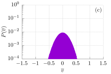
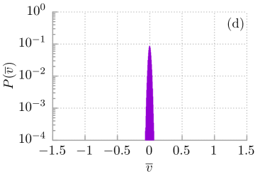
Figure 3: The probability distributions $P(\overline{v})$ for the time averaged velocity $\overline{v}$ of the Brownian particle in the deterministic limit of vanishing temperature $Q=0$ and noisy dynamics $Q=0.5$ are depicted in left and right panels, respectively. Upper plots ((a) and (c)) represent the first maximum ($a=9.8$) in diffusion oscillations whereas bottom ones ((b) and (d)) correspond to the first minimum ($a=15.3$). Other parameters are the same as in Fig. 2.

IV Description of the simulations

The complexity of stochastic dynamics determined by Eq. (6) with three-dimensional phase space $\{x,y=\dot{x},z=\omega t\}$ is rooted in the four-dimensional parameter space $\{\gamma,a,\omega,Q\}$. The Fokker-Planck equation corresponding to Eq. (6) cannot be solved analytically and for this reason we had to resort to comprehensive numerical simulations. All calculations have been done using a Compute Unified Device Architecture (CUDA) environment implemented on a modern desktop Graphics Processing Unit (GPU). This proceeding allowed for a speedup of factor of the order $10^{3}$ times as compared to present day Central Processing Unit (CPU) method spiechowicz2015cpc . The Langevin equation (6) were integrated using a second order predictor-corrector scheme platen with the time step $h=10^{-2}$. The quantities characterizing diffusive behaviour of the system were averaged over the ensemble of $N=2^{14}=16384$ trajectories, each starting with different initial conditions $x(0)$ and $v(0)$ distributed uniformly over the intervals $[0,2\pi]$ and $[-2,2]$, respectively. Under the assumption of asymptotic normality of the estimator of the mean of the quantities characterizing diffusive behavior of our system, we obtain that the statistical error of the Monte Carlo simulation is of the order of $\approx 10^{-2}$, which seems adequate for our purposes. The time span of simulations read $10^{6}$ periods $2\pi/\omega$ of the external driving $a\cos{(\omega t)}$ and was extensive enough to reach the long time limit indicated by the stationarity of diffusion coefficient.

V Oscillations of the diffusion coefficient

The spatially periodic potential and the ac-driving are reflection symmetric with respect to coordinate and time, respectively. Therefore in the long time limit the averaged particle velocity is zero $\langle\overline{v}\rangle=0$ and no directed transport can be generated in the studied system. Moreover, for non-zero temperature $Q>0$ the diffusion is normal in the long time limit and therefore its coefficient $D$ is well-defined (i.e. it has a finite value larger than zero). In some regimes of the parameter space $D$ can render a non-trivial behavior. E.g. the Einstein relation fails and non-monotonic temperature dependence of the diffusion coefficient can be detected. Because the ac-driving takes the system out of thermal equilibrium the influence of its parameters $a$ and $\omega$ on $D$ is expected to be particularly interesting. In Fig. 1 we depict the dependence of the rescaled diffusion coefficient $D/D_{0}$ on the ac-driving amplitude $a$, where $D_{0}$ corresponds to free thermal diffusion $D_{0}=Q/\gamma$. One can notice there two distinctive features, namely, (i) this quantity exhibits giant damped quasiperiodic oscillations as $a$ increases and (ii) the maximal value of $D$ is several decades larger than the Einstein diffusion coefficient $D_{0}$. E.g. for $\omega=2$, the nonequilibrium diffusion coefficient is $D\approx 30D_{0}$. Similar oscillations of diffusion has been observed in other systems. In Ref. peter-epl, , the overdamped Brownian particle moves in a sawtooth potential and is driven by a time-periodic piecewise constant driving force. The diffusion coefficient is also periodically damped with respect to the ”tilting time” (the time when the driving force is non-zero) and the maximal amplification is $D\approx 14D_{0}$. In Ref. march-prl, , the overdamped limit of the dynamics (6) was considered and the authors found oscillations of diffusion with its maximal value reading $D\approx D_{0}$. These results should be contrasted with giant variability of the latter quantity reported here in which it changes by two orders of magnitude for the full inertial dynamics characterized by the term $M\ddot{x}$ in Eq. (1).

Let us now explain the mechanism of the observed oscillatory diffusive behavior. For this purpose we first consider a fixed set of parameters with $\omega=2$ for which this effect is the most prominent, see Fig. 2. We present there the rescaled diffusion coefficient $D/D_{0}$ (panel (a)) together with the variance $\sigma_{\overline{v}}^{2}$ (panel (b)) of the time averaged velocity as a function of the ac-driving amplitude $a$. Unexpectedly, the behavior of $D/D_{0}$ and $\sigma^{2}_{\overline{v}}$ is very similar. The subsequent maxima and minima are located at the same value of the amplitude, $a_{1}=9.8,a_{2}=15.3,a_{3}=22,a_{4}=28.2$. The reader can conclude that the magnitude of $D/D_{0}$ is strictly related to the spread of time averaged velocity measured by the variance $\sigma_{\overline{v}}^{2}$. Larger fluctuations of time averaged velocity lead to greater span of particle trajectories and consequently to superior diffusion coefficient. We note that the difference in $\sigma_{\overline{v}}^{2}$ corresponding to the first maximum ($a=9.8$) and minimum ($a=15.3$) is notable and equals almost two orders of magnitude.

In the next step we consider deterministic $Q=0$ and noisy dynamics $Q=0.5$ for two values of the ac-driving amplitude $a$ characterizing the first maximum ($a=9.8$) and subsequent minimum ($a=15.3$). In Fig. 3 we present the corresponding probability distributions $P(\overline{v})$ for the time averaged velocity $\overline{v}$ of the Brownian particle. In the deterministic case $Q=0$, there are two classes of trajectories in this parameter regime, namely, the running solutions (the motion is unbounded in space) and the locked solutions (the particle is trapped in the potential well). We note that for the noisy dynamics with $Q=0.5$ fluctuations of time averaged velocity are much larger for the first maximum ($a=9.8$) than for the subsequent minimum ($a=15.3$). This observation confirms the result presented in Fig. 2. In left panels of Fig. 3 we depict the same characteristics but now for the deterministic system with $Q=0$. The reader can detect there the multistable dynamics: the locked states with $\overline{v}=0$ coexist with a family of running ones $\overline{v}\neq 0$. Since the system given by Eq. (6) is symmetric and the directed transport must vanish $\langle\overline{v}\rangle\equiv 0$ the running solutions can occur only in pairs $\overline{v}=\pm\overline{v}_{i}$.

A typical single trajectory of the noisy system with $Q>0$ contains: (i) extended periods when the particle is locked in one or several potential wells and (ii) time intervals when it is running. Therefore non-zero thermal noise activates transitions between the states coexisting for the deterministic system. For such multistable velocity dynamics there are three contributions to spread of trajectories of the system and consequently to the diffusion coefficient $D$. The first, which is the leading one, comes from the spread associated with relative distance between the locked and running trajectories. The second and third parts correspond to thermally driven spread of trajectories following the locked and running solutions, respectively. The magnitude of these three contributions are related to stationary probabilities $p_{0}$ and $p_{r}$ of the particle to reside onto the locked and running trajectories, respectively. In the noisy case with dimensionless temperature $Q=0.5$ (which is rather ”high” temperature) the given particle trajectory is classified as the locked if the corresponding time average velocity $\overline{v}\approx 0$. In the case $\overline{v}\neq 0$ it is categorized as the running one. It allows to reformulate the diffusion coefficient $D$ in terms of them. It is expected to be maximal when the share of the first contribution associated with the spread between the locked and running solutions is peaked.

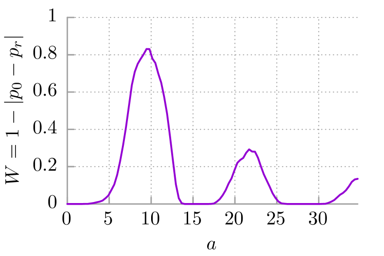
Figure 4: The quantifier $W=1-|p_{0}-p_{r}|$ characterizing the difference in number of locked and running trajectories is depicted as a function of the ac-driving amplitude $a$. Other parameters are the same as in Fig. 2.

To this aim, let us define the quantifier $W=1-|p_{0}-p_{r}|$ which describes the difference in number of locked and running trajectories. If $W\neq 0$ then these two classes of solutions coexist. When $p_{0}=p_{r}$ the quantifier is maximal $W=1$. It corresponds to the situation in which locked and running trajectories are equiprobable. In Fig. 4 we depict $W$ as a function of the ac-driving amplitude $a$. The reader can observe that the maxima of this curve are exactly at the same points as the corresponding ones for the diffusion coefficient $D$, c.f. Fig. 1 for $\omega=2$. Moreover, the second maximum is significantly smaller than the first one and this fact is translated into the minor second maximum in the dependence of diffusion coefficient $D$. Therefore we can conclude that the giant damped quasiperiodic diffusion oscillations observed in Fig. 1 can be characterized by the quantifier $W$ which describes the share of the spread of trajectories coming from the relative distance between the locked and running trajectories.

VI Conclusions

In this work we revisited the problem of diffusion in driven periodic system. As a particular instance we picked a paradigmatic model of the Brownian particle dwelling in a periodic potential and subjected to an external time periodic force. Since the latter takes the analyzed system out of equilibrium it is expected to possess the impact on its diffusive properties. Indeed, in this work we detected a peculiar effect of giant damped quasiperiodic diffusion oscillations controlled by the amplitude of external driving force. As a mechanism of this phenomenon we identified the corresponding oscillations of difference in the number of of locked and running solutions which carries the leading contribution to the spread of system trajectories, time averaged velocities and consequently also to the diffusion coefficient.

Our findings can be viewed as another manifestation of the impact of the dynamics in the velocity subspace onto the kinetics in the coordinate subspace. Recently it has been discovered that similar interplay may be also modus operandi of fluctuation-induced dynamical localization spiechowicz2017scirep ; spiechowicz2019chaos causing anomalous diffusion in systems which at the first glance should not react in this way. The problem how the directed transport influences the diffusive behavior is largely unexplored and therefore we expect new instances of it to appear in the near future, including also the experimental ones. It is facilitated by the fact that the considered system has a multitude of physical realizations risken with Josephson junctions and cold atoms dwelling in optical lattices. E.g., for a system consisting of a resistively and capacitively shunted Josephson junction device, the coordinate $x(t)$ corresponds to the phase difference $\phi(t)$ between the macroscopic wave functions of the Cooper pairs on both sides of the Josephson junction and the velocity $v(t)$ corresponds to the voltage $V(t)$ across the junction. Because it would be difficult to measure diffusion of the phase instead of it experimentalists can measure the voltage fluctuations from which they can extract information on diffusion of the phase. Finally, our findings can be used for control of diffusion according to the procotol presented in Fig. 2: if large diffusion is desired one has to find a value of the amplitude $a$ (here $a=9.8)$ which maximizes $D$. In turn, if one needs to reduce diffusion the suitable value of $a$ (here $a=15.3$) should be matched to minimalize the diffusion coefficient. Moreover, at the maximum $D_{max}\approx 30D_{0}>D_{0}$ and at the minimum $D_{min}\approx 0.3D_{0}<D_{0}$, i.e. $D_{max}\approx 100D_{min}$ and one can control diffusion over the range of two orders of magnitude.

References

References

- (1) R. Benzi, A. Sutera and A. Vulpiani, J. Phys. A.: Math. Gen. 14, L453 (1981)
- (2) L. Gammaitoni, P. Hänggi, P. Jung and F. Marchesoni, Rev. Mod. Phys. 70, 223 (1998)
- (3) A. Pikovsky and J. Kurths, Phys. Rev. Lett. 78, 775 (1997)
- (4) B. Lindner, J. Garcia-Ojalvo, A. Neiman and L. Schimansky-Geier, Phys. Rep. 392, 321 (2004)
- (5) P. Hänggi, F. Marchesoni, Rev. Mod. Phys. 81, 387 (2009)
- (6) C. J. Olson Reichhardt, C. Reichhardt, Annu. Rev. Condens. Matter Phys. 8, 51 (2017)
- (7) L. Machura, M. Kostur, P. Talkner, J. Łuczka and P. Hänggi, Phys. Rev. Lett. 98, 040601 (2007)
- (8) J. Nagel, D. Speer, T. Gaber, A. Sterck, R. Eichhorn, P. Reimann, K. Ilin, M. Siegel, D. Koelle and R. Kleiner, Phys. Rev. Lett. 100, 217001 (2008)
- (9) A. Slapik, J. Łuczka, P. Hänggi, J. Spiechowicz, Phys. Rev. Lett. 122, 070602 (2019)
- (10) J. Spiechowicz, P. Hänggi and J. Łuczka, New J. Phys. 21, 083029 (2019)
- (11) R. Klages, G. Radons and I. M. Sokolov, Anomalous Transport: Foundations and Applications (Wiley-VCH, 2008)
- (12) R. Metzler, J. H. Jeon, A. G. Cherstvy and E. Barkai, Phys. Chem. Chem. Phys. 16, 24128 (2014)
- (13) I. G. Marchenko and I. I. Marchenko, Europhys. Lett. 100, 50005 (2012)
- (14) J. Spiechowicz, P. Talkner, P. Hänggi and J. Łuczka, New J. Phys. 18, 123029 (2016)
- (15) I. G. Marchenko, I. I. Marchenko, V. I. Tkachenko, JETP Letters 106, 242 (2017)
- (16) J. Spiechowicz, M. Kostur and J. Łuczka, Chaos 27, 023111 (2017)
- (17) I. G. Marchenko, I. I. Marchenko and A. V. Zhiglo, Phys. Rev. E 97, 012121 (2018)
- (18) I. G. Marchenko, I. I. Marchenko and V. I. Tkachenko, JETP Letters 109, 671 (2019)
- (19) A. Crossman, Understanding Diffusion in Sociology. ThoughtCo, Feb. 16, (2021); web-link: thoughtco.com/cultural-diffusion-definition-3026256
- (20) M. C. Marchetti, J. F. Joanny, S. Ramaswamy, T. B. Liverpool, J. Prost, M. Rao and R. A. Simha, Rev. Mod. Phys. 85, 1143 (2013)
- (21) J. Spiechowicz, P. Hänggi and J. Łuczka, Phys. Rev. E 90, 032104 (2014)
- (22) C. Bechinger, R. Di Leonardo, H. Löwen, C. Reichhardt, G. Volpe and G. Volpe, Rev. Mod. Phys. 88, 045006 (2016)
- (23) F. S. Gnesotto, F. Mura, J. Gladrow and C. P. Broedersz, Rep. Prog. Phys. 81, 066601 (2018)
- (24) B. Wang, J. Kuo, S. C. Bae, and S. Granick, Nat. Mater. 11, 481 (2012)
- (25) A. V. Chechkin, F. Seno, R. Metzler, and I. M. Sokolov, Phys. Rev. X 7, 021002 (2017)
- (26) K. Bialas, J. Łuczka, P. Hänggi, and J. Spiechowicz, Phys. Rev. E 102, 042121 (2020)
- (27) R. Kubo, Rep. Prog. Phys. 29, 255 (1966)
- (28) R. L. Kautz, Rep. Prog. Phys. 59, 935 (1996)
- (29) J. Spiechowicz and J. Łuczka J Chaos 25, 053110 (2015)
- (30) J. A. Blackburn, M. Cirillo, N. Gronbech-Jensen, Phys. Rep. 611, 120 2016)
- (31) S. Denisov, S. Flach, and P. Hänggi, Phys. Rep. 538, 77 (2014)
- (32) E. Lutz and F. Renzoni, Nat. Phys. 9, 615 (2013)
- (33) F. Kindermann et al., Nat. Phys. 13, 137 (2017)
- (34) J. Spiechowicz, J. Łuczka, P. Hänggi, Sci. Rep. 6, 30948 (2016)
- (35) J. Spiechowicz, M. Kostur and Ł. Machura, Comp. Phys. Commun. 191, 140 (2015)
- (36) E. Platen and N. Bruti-Liberati, Numerical Solution of Stochastic Differential Equations with Jumps in Finance, (Springer, 2011)
- (37) M. Schreier, P. Reimann, P. Hänggi and E. Pollak, Europhys. Lett. 44, 416 (1998)
- (38) M. Borromeo and F. Marchesoni, Phys. Rev. Lett. 99, 150605 (2007)
- (39) J. Spiechowicz and J. Łuczka, Sci. Rep. 7, 16451 (2017)
- (40) J. Spiechowicz and J. Łuczka, Chaos 29, 013105 (2019)
- (41) H. Risken, The Fokker-Planck Equation: Methods of Solution and Applications (Springer, 1996)