Robust Interaction-Enhanced Sensing via Antisymmetric Rabi Spectroscopy

Abstract

Atomic spectroscopy, an essential tool for frequency estimation, is widely used in quantum sensing. Atom-atom interaction can be used to generate entanglement for achieving quantum enhanced sensing. However, atom-atom interaction always induces collision shift, which brings systematic error in determining the resonance frequency. Contradiction between utilizing atom-atom interaction and suppressing collision shift generally exists in atomic spectroscopy. Here, we propose an antisymmetric Rabi spectroscopy protocol without collision shift in the presence of atom-atom interactions. We analytically find that the antisymmetric point can be used for determining the resonance frequency. For small Rabi frequency, our antisymmetric Rabi spectroscopy with slight atom-atom interaction can provide better measurement precision than the conventional Rabi spectroscopy. With stronger atom-atom interaction and Rabi frequency, the spectrum resolution can be dramatically improved and the measurement precision may even beat the standard quantum limit. Moreover, unlike the quantum-enhanced Ramsey interferometry via spin squeezing, our scheme is robust against detection noises. Our antisymmetric Rabi spectroscopy protocol has promising applications in various practical quantum sensors such as atomic clocks and atomic magnetometers.

Introduction. – Atomic spectroscopy, the basis for precise measurement of transition frequencies, has been extensively applied in fundamental sciences as well as high-precision sensors [1]. Most quantum sensors employ a pair of discrete energy levels relevant to the physical quantity to be measured. By using atomic spectroscopy to determine the transition frequency, one can estimate the physical quantity to be measured [2] and build various practical quantum sensors such as atomic clocks [3, 4, 5], magnetometers [6, 7, 8], gyroscopes [9] and gravimeters [10]. On one hand, atom-atom interaction can be used to generate the desired entanglement for improving the measurement precision from the standard quantum limit (SQL) to the Heisenberg limit (HL) [11, 12, 13, 14, 15]. On the other hand, in atomic spectroscopy [16, 17, 18, 19], atom-atom interaction always results in collision shift [20] which brings systematic error in determining the resonance frequency [21]. Many schemes have been developed to suppress the influences of atom-atom collisions [22, 23, 24].

Generally, in high-precision quantum sensing via atomic spectroscopy, there is a contradiction between utilizing atom-atom interaction and suppressing collision shift. To achieve high-precision Ramsey spectroscopy, one can use atom-atom interaction to prepare the desired entanglement and then turn off atom-atom interaction for interrogation. In this way, the collision shift can be small, but it requires precise time-dependent manipulation of atom-atom interactions. In Rabi spectroscopy, the coupling field and the atom-atom interaction coexist. It has been demonstrated that one may achieve a Rabi spectroscopy towards the HL with two correlated ions [25]. However, in such a protocol, the system should be split into two orthogonal subspaces with different parities as different probes, which adds additional complexity to the existing Rabi protocols. Therefore, it starves for an efficient spectroscopy protocol without collision shift and meanwhile one can utilize atom-atom interactions to improve the measurement precision beyond the SQL.

In this Letter, we propose a robust interaction-enhanced frequency estimation protocol via antisymmetric Rabi spectroscopy. Instead of preparing all atoms in the lower level for the conventional Rabi spectroscopy, our protocol inputs an equal superposition state of the two sensor levels before applying the coupling field for implementing Rabi oscillation. We analytically find that the Rabi spectrum becomes exactly antisymmetric with respect to the detuning in the presence of atom-atom interactions. This means the absence of collision shift in our protocol theoretically. In practice, the desired input state can be generated by applying a short $\pi/2$ pulse and the antisymmetric point can still appear even under atom-atom interaction. For small Rabi frequency, our protocol with slight atom-atom interaction can offer better measurement precision. More importantly, the measurement precision can be improved beyond the SQL by using stronger atom-atom interaction and Rabi frequency. Compared to the spin-squeezing-enhanced Ramsey spectroscopy protocol, our scheme is much more robust against detection noises.

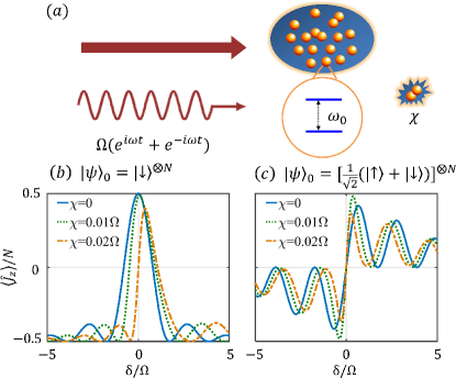
Figure 1: (Color online) (a) Schematic of a quantum sensor via Rabi oscillation. A laser field interacts with an ensemble of interacting atoms. $\Omega$ denotes the Rabi frequency, $\omega$ is the laser frequency, $\omega_{0}$ is the atomic transition frequency to be measured, and $\chi$ denotes the atom-atom interaction. (b) The final population difference versus the detuning $\delta$ for the initial state $|\psi\rangle_{0}=|\pi,0\rangle_{SCS}$. (c) The final population difference versus the detuning $\delta$ for the initial state $|\psi\rangle_{0}=|\pi/2,0\rangle_{SCS}$, which can be realized by applying a short $\pi/2$ pulse along $y$ axis on $|\pi,0\rangle_{SCS}$. Here, the atom number $N=100$ and the total evolution time $T$ satisfying $\Omega T=\pi$. The blue (solid), green (dashed) and orange (dash-dotted) lines are the results with $\chi=0$, $0.01\Omega$ and $0.02\Omega$, respectively.

Conventional Rabi oscillation in an atomic ensemble. – We consider an ensemble of $N$ two-level atoms, which can be regraded as identical pseudospin-$\frac{1}{2}$ particles obeying a collective spin $\hat{J}$ with $\hat{J}_{x}=\sum_{n=1}^{N}\sigma_{x}^{(n)}$, $\hat{J}_{y}=\sum_{n=1}^{N}\sigma_{y}^{(n)}$, and $\hat{J}_{z}=\sum_{n=1}^{N}\sigma_{z}^{(n)}$. Here $\sigma_{x,y,z}^{(n)}$ denotes the Pauli matrices for the $n$-th atom. In the Schwinger representation, $\hat{J_{x}}=\frac{1}{2}(\hat{a}^{{\dagger}}\hat{b}+\hat{b}^{{\dagger}}\hat{a})$, $\hat{J_{y}}=\frac{i}{2}(\hat{a}^{{\dagger}}\hat{b}-\hat{b}^{{\dagger}}\hat{a})$, $\hat{J_{z}}=\frac{1}{2}(\hat{b}^{{\dagger}}\hat{b}-\hat{a}^{{\dagger}}\hat{a})$ , where $\hat{a}$ and $\hat{b}$ are the annihilation operators for atoms in $\left|\uparrow\right\rangle$ and $\left|\downarrow\right\rangle$, respectively. These collective spin operators obey the general angular momentum commutation relations $[\hat{J_{i}},\hat{J_{j}}]=i\hbar\epsilon_{ijk}\hat{J_{k}}$ with $i,j,k=x,y,z$ and $\epsilon_{ijk}$ the Levi-Civita symbol. Thus, an arbitrary state can be expressed by $|\Psi\rangle=\sum_{m=-N/2}^{N/2}C_{m}|J,m\rangle$, where $|J,m\rangle$ is the Dicke basis denoting $(N/2-m)$ atoms in $\left|\uparrow\right\rangle$ and $(N/2+m)$ atoms in $\left|\downarrow\right\rangle$.

A well-known spectroscopic method for frequency estimation is implementing Rabi oscillations. In a non-interacting atomic ensemble driven by an external coupling field, its Rabi oscillations obey the Hamiltonian $\hat{H}=\omega_{0}\hat{J_{z}}+\Omega(e^{i\omega t}+e^{-i\omega t})\hat{J_{x}}$, where $\omega_{0}$ is the atomic transition frequency, $\omega$ is the frequency of the coupling field, and $\Omega$ is the Rabi frequency. For simplicity we set $\hbar=1$ hereafter. In the rotating-frame with rotating-wave approximation (RWA), the Hamiltonian becomes

$$\hat{H}_{R}=\Omega\hat{J_{x}}+\delta\hat{J_{z}},$$ (1)

where the detuning $\delta=\omega_{0}-\omega$. Without atom-atom interactions, the system state can be described by a spin coherent state (SCS) $\left|\theta,\phi\right\rangle_{SCS}=\left(\cos\theta/2\left|\uparrow\right\rangle+e^{i\phi}\sin\theta/2\left|\downarrow\right\rangle\right)^{\otimes N}$, in which all atoms are in the same quantum state. Conventionally, one prepare an initial SCS $\left|\psi\right\rangle_{0}=\left|\pi,0\right\rangle_{SCS}=\left(\left|\downarrow\right\rangle\right)^{\otimes N}$ with all atoms in $\left|\downarrow\right\rangle$. Then, the initial state evolves according to $\left|\psi(t)\right\rangle=e^{-i\hat{H}_{R}t}\left|\pi,0\right\rangle_{SCS}$. At time $T$, we have the half population difference

$$\langle\hat{J_{z}}(T)\rangle=-\frac{N}{2}\frac{\delta^{2}+\Omega^{2}\cos(\sqrt{\Omega^{2}+\delta^{2}}T)}{\Omega^{2}+\delta^{2}},$$ (2)

which is a symmetric function with respect to $\delta=0$. In practice, one would choose $\Omega T=\pi$ and measure the half population difference $\langle\hat{J_{z}}(T)\rangle$. It attains the maximum at $\delta=0$ so that can be used as the frequency locking signal, see the blue solid line in Fig. 1 (b).

Taking into account the atom-atom interaction, the original Hamiltonian becomes $\hat{H}^{\prime}=\omega_{0}\hat{J_{z}}+\chi\hat{J}_{z}^{2}+\Omega(e^{i\omega t}+e^{-i\omega t})\hat{J_{x}}$, where $\chi$ characterizes the strength of effective atom-atom interaction [see Fig. 1 (a)]. In the rotating-frame with RWA, the Hamiltonian reads

$$\hat{H}_{R}^{\prime}=\Omega\hat{J_{x}}+\chi\hat{J}_{z}^{2}+\delta\hat{J_{z}}.$$ (3)

When $\chi$ is non-negligible, the atomic collision causes a frequency shift and the locking signal is no longer symmetric with $\delta=0$. For example, when $\chi=0.01\Omega$, an obvious frequency shift can be observed, see the green dashed line in Fig. 1 (b). While for $\chi=0.02\Omega$, the frequency shift is larger and the lineshape also distorted, see the orange dash-dotted line in Fig. 1 (b).

In the conventional Rabi spectroscopy, the atom-atom interaction always induces a collision shift that decreasing the accuracy for estimating the transition frequency. Besides, since the maximum is around $\delta=0$, its signal slope equals zero and the standard deviation $\Delta\delta$ at this point is diverged. In general, it is necessary to find out two symmetric points (with respect to $\delta=0$) to determine the on-resonance point. These limit the performances of the Rabi spectroscopy. Below, we analytically analyze the quantum sensing via antisymmetric Rabi spectroscopy and demonstrate how to achieve better frequency estimation at the on-resonance point $\delta=0$.

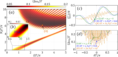
Figure 2: (Color online) (a) The measurement precision $\Delta\omega_{0}$ at the on-resonance point versus the Rabi frequency $\Omega$ and the atom-atom interaction $\chi$ for a fixed evolution time $T=1$. (b) The enlarged area of the dotted box in (a). (c) The scaled population difference $\langle\hat{J_{z}}(T)\rangle/N$ and (d) the measurement precision $\Delta\omega_{0}$ versus the detuning $\delta$ for the points I (green circle, $\Omega=\pi,\chi=0$), II (blue triangle, $\Omega=\pi,\chi=0.4\pi/N$) and III (orange square, $\Omega=3\pi,\chi=6\pi/N$). Here, the total atom number $N=100$ and the initial state $|\psi\rangle_{0}=|\pi/2,0\rangle_{SCS}$.

Antisymmetric Rabi spectroscopy. – Let’s turn back to the non-interacting case ($\chi=0$). For the Rabi oscillation from an arbitrary initial state $|\psi\rangle_{0}$, we analytically obtain its half population difference $\langle\hat{J}_{z}(T)\rangle$ at time $T$,

$$\langle\hat{J}_{z}(T)\rangle=\langle\psi(T)|\hat{J_{z}}|\psi(T)\rangle=_{0}\!\!\langle\psi|e^{i\hat{H}_{R}T}\hat{J_{z}}e^{-i\hat{H}_{R}T}|\psi\rangle_{0}$$

$$=\langle\hat{J_{x}}\rangle_{0}\left(\sum_{k=1}^{\infty}\frac{1}{(2k)!}x_{2k}\right)+\langle\hat{J_{y}}\rangle_{0}\left(\sum_{k=1}^{\infty}\frac{1}{(2k-1)!}y_{2k-1}\right)$$

$$~{}~{}+\langle\hat{J_{z}}\rangle_{0}\left(1+\sum_{k=1}^{\infty}\frac{1}{(2k)!}z_{2k}\right)$$

$$=\langle\hat{J_{x}}\rangle_{0}X(\Omega,\delta,T)\!+\!\langle\hat{J_{y}}\rangle_{0}Y(\Omega,\delta,T)\!+\!\langle\hat{J_{z}}\rangle_{0}Z(\Omega,\delta,T),$$ (4)

where $y_{1}=\Omega T$, $x_{2k}=y_{2k-1}(\delta T)$, $z_{2k}=-y_{2k-1}(\Omega T)$ and $y_{2k-1}=-(\delta T)x_{2k}+(\Omega T)z_{2k}$ for $k>1$. The sums $X(\Omega,\delta,T)=\frac{\Omega\delta}{\Omega^{2}+\delta^{2}}\left[1-\cos(\sqrt{\Omega^{2}+\delta^{2}}T)\right]$, $Y(\Omega,\delta,T)=\frac{\Omega\sin(\sqrt{\Omega^{2}+\delta^{2}}T)}{\sqrt{\Omega^{2}+\delta^{2}}}$, and $Z(\Omega,\delta,T)=\frac{\delta^{2}+\Omega^{2}\cos(\sqrt{\Omega^{2}+\delta^{2}}T)}{\Omega^{2}+\delta^{2}}$ can be analytically calculated, see more details [26]. If $|\psi\rangle_{0}=|\pi,0\rangle_{SCS}$, we have $\langle\hat{J_{z}}\rangle_{0}=-\frac{N}{2}$ and $\langle\hat{J_{x}}\rangle_{0}=\langle\hat{J_{y}}\rangle_{0}=0$ and Eq. (Robust Interaction-Enhanced Sensing via Antisymmetric Rabi Spectroscopy) gives Eq. (2).

According to Eq. (Robust Interaction-Enhanced Sensing via Antisymmetric Rabi Spectroscopy), one can analytically give the relation between the half population difference $\langle\hat{J}_{z}(T)\rangle$ and the detuning $\delta$ for any initial state $|\psi\rangle_{0}$. Since $X(\Omega,\delta,t)=-X(\Omega,-\delta,t)$, $Y(\Omega,\delta,t)=Y(\Omega,-\delta,t)$ and $Z(\Omega,\delta,t)=Z(\Omega,-\delta,t)$, we find that, when $\langle\hat{J_{z}}\rangle_{0}=\langle\hat{J_{y}}\rangle_{0}=0$, the half population difference $\langle\hat{J}_{z}(T)\rangle=\frac{\Omega\delta}{\Omega^{2}+\delta^{2}}\left[1-\cos(\sqrt{\Omega^{2}+\delta^{2}}T)\right]\langle\hat{J_{x}}\rangle_{0}$ is exactly antisymmetric with respect to $\delta=0$. For an example, inputting the initial state $|\psi\rangle_{0}=|\pi/2,0\rangle_{SCS}$ whose $\langle\hat{J_{x}}\rangle_{0}=\frac{N}{2}$ and $\langle\hat{J_{z}}\rangle_{0}=\langle\hat{J_{y}}\rangle_{0}=0$, we have

$$\langle\hat{J}_{z}(T)\rangle=\frac{N}{2}\frac{\Omega\delta}{\Omega^{2}+\delta^{2}}\left[1-\cos(\sqrt{\Omega^{2}+\delta^{2}}T)\right].$$ (5)

Eq. (5) is an antisymmetric function of $\delta$ for arbitrary $\Omega$ and $T$, see the blue solid line in Fig. 1 (c). The measurement precision can be calculated as

$$\Delta\omega_{0}=\frac{\Delta\hat{J}_{z}}{|\partial\langle\hat{J}_{z}\rangle/\partial\omega_{0}|}=\frac{\Delta\hat{J}_{z}}{|\partial\langle\hat{J}_{z}\rangle/\partial\delta|}.$$ (6)

Compared to the conventional Rabi spectroscopy with $|\psi\rangle_{0}=|\pi,0\rangle_{SCS}$, the slope of the signal at on-resonance point $\delta=0$ becomes sharp and the corresponding measurement precision becomes high [19, 27].

Amazingly, in the presence of atom-atom interaction, there is no collision shift in the antisymmetric Rabi spectroscopy. We find that the frequency locking signal is always antisymmetric with respect to $\delta=0$ in the presence of $\chi$, see Fig. 1 (c). Since the antisymmetry of the signal preserves with $\chi$, the antisymmetric point has no collision shift theoretically and can be used as the on-resonance point.

The key for antisymmetric Rabi spectroscopy originates the symmetry of Hamiltonian (3) [28, 29, 30]. Under the transformation $\hat{a}(\hat{b})\rightarrow\hat{b}(\hat{a})$, we have $\hat{J}_{x}\rightarrow\hat{J}_{x}$ and $\hat{J}_{z}\rightarrow-\hat{J}_{z}$. The first two terms $\Omega\hat{J_{x}}$ and $\chi\hat{J}_{z}^{2}$, which have even parity symmetry, are invariant under the transformation of exchanging $\left|\uparrow\right\rangle$ and $\left|\downarrow\right\rangle$. The last term $\delta\hat{J_{z}}$, which has odd parity symmetry, changes according to $\delta\hat{J}_{z}\rightarrow-\delta\hat{J}_{z}$ when $\left|\uparrow\right\rangle\rightarrow\left|\downarrow\right\rangle$. For an initial state $|\psi\rangle_{0}=\sum_{m=-J}^{J}C_{m}(0)|J,m\rangle$ with $C_{m}(0)=C_{-m}(0)$ (e.g. $|\psi\rangle_{0}=|\pi/2,0\rangle_{SCS}$), when $\delta=0$, the evolved state will always possess even parity symmetry (that is $C_{m}(t)=C_{-m}(t)$) [26]. Thus, the half population difference $\langle\hat{J}_{z}(t)\rangle=\sum_{m=-J}^{J}m|C_{m}(t)|^{2}=0$ at the on-resonance point $\delta=0$. However, if $\delta\neq 0$, $\delta\hat{J}_{z}$ and $-\delta\hat{J}_{z}$ rotate along opposite directions, which results in the antisymmetry property $\langle\hat{J}_{z}(\delta,t)\rangle=-\langle\hat{J}_{z}(-\delta,t)\rangle$.

Theoretically, one can write the time-evolution in the interaction picture

$$i\frac{d}{dt}|\psi(t)\rangle^{I}=\hat{H}_{I}|\psi(t)\rangle^{I},$$ (7)

where $\hat{H}_{I}=e^{i\hat{H}_{0}t}\Omega\hat{J}_{x}e^{-i\hat{H}_{0}t}=\frac{\Omega}{2}\left(\hat{J}_{+}^{I}+\hat{J}_{-}^{I}\right)$ with $H_{0}=\chi\hat{J}_{z}^{2}+\delta\hat{J}_{z}$ and $\hat{J}_{\pm}^{I}=\hat{J}_{\pm}e^{i\chi t}e^{\pm i(\delta t+2\chi t\hat{J}_{z})}$. $|\psi(t)\rangle^{I}=e^{i\hat{H}_{0}t}|\psi(t)\rangle=\sum_{m=-N/2}^{N/2}C_{m}^{I}(t)|J,m\rangle$ with $|\psi(t)\rangle=\sum_{m=-N/2}^{N/2}C_{m}(t)|J,m\rangle$. Substituting $|\psi(t)\rangle^{I}$ into Eq. (S31), one can find ${C}_{m}^{I}(\delta,t)={C}_{-m}^{I}(-\delta,t)$ and the population difference $\langle\hat{J}_{z}(\pm\delta,t)\rangle=\pm\sum_{m=-J}^{J}m|C_{m}^{I}(\delta,t)|^{2}$ if $C_{m}(0)=C_{-m}(0)$ (see the detailed proof [26]). Thus spectrum is antisymmetric versus the detuning.

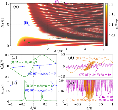
Figure 3: (Color online) (a) The measurement precision $\Delta\omega_{0}$ at the on-resonance point versus the evolution time $T$ and the atom-atom interaction $\chi$ for a fixed Rabi frequency $\Omega$. Here, $\Omega=1$. (b) The scaled population difference $\langle\hat{J_{z}}(T)\rangle/N$ and (c) the measurement precision $\Delta\omega_{0}$ versus the detuning $\delta$ for the points I (green circle, $T=\pi,\chi=1/N$), II (blue triangle, $T=\pi,\chi=5/N$). (d) The scaled population difference $\langle\hat{J_{z}}(T)\rangle/N$ and (e) the measurement precision $\Delta\omega_{0}$ versus the detuning $\delta$ for the points III (orange square, $T=3\pi,\chi=2/N$), IV (purple reversed triangle, $T=3\pi,\chi=10/N$). Here, the total atom number $N=100$ and the initial state $|\psi\rangle_{0}=|\pi/2,0\rangle_{SCS}$.

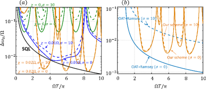
Figure 4: (Color online) The robustness against detection noises. Here, $\sigma$ characterizes the detection noise strength. (a) The measurement precision $\Delta\omega_{0}$ versus the evolution time $T$ for a fixed Rabi frequency $\Omega=1$ without and with detection noises. The solid and dashed lines correspond to our scheme with $\sigma=0$ and $\sigma=\sqrt{N}$, respectively. The black solid line denotes the standard quantum limit. (b) Comparison between our scheme and the Ramsey scheme with spin squeezing. For the Ramsey scheme, we consider the optimal squeezing with $T_{p}=3^{1/6}N^{-2/3}/\chi$ and the interrogation time $T_{R}=T-T_{p}$. Here, for both our scheme and the Ramsey scheme, $\Omega=1$ and $\chi=2/N$ with the total atom number $N=100$.

Interaction-enhanced sensing via antisymmetric Rabi spectroscopy.– We choose the non-entangled SCS $|\psi\rangle_{0}=|\pi/2,0\rangle_{SCS}$ as the input state. First, for sensors based on Rabi spectroscopy, such as optical lattice clocks [31, 20, 32, 33, 34, 35], our antisymmetric Rabi spectroscopy with slight atom-atom interaction can enhance the measurement precision. In Fig. 2 (b), the measurement precision at the on-resonance point with atom-atom interaction (point II, $\chi=0.004\pi$ with $N=100$) is better than the one without atom-atom interaction (point I, $\chi=0$) in the same condition of $\Omega T=\pi$. The scaled half population difference with atom-atom interaction exhibits sharper slope at the antisymmetric point, resulting in the better measurement precision, see Fig. 2 (c) and (d).

Second, for a fixed evolution time $T=1$, as Rabi frequency $\Omega$ and atom-atom interaction $\chi$ increase, the measurement precision at the on-resonance point may be further enhanced. For example with $\Omega T=3\pi$ and $\chi=0.06\pi$ [the point III in Fig. 2 (a)], the measurement precision is much higher than the ones of points I and II in Fig. 2 (b). The signal $\langle\hat{J}_{z}(T)\rangle$ exhibits a series of oscillations around the on-resonance point resulting in high resolution and measurement precision, as shown in Fig. 2 (c) and (d). Further, we fix Rabi frequency $\Omega=1$ and show how the measurement precision depends on atom-atom interaction $\chi$ and evolution time $T$, see Fig. 3 (a). For a fixed $\chi$, the measurement precision oscillates with evolution time and there exists an optimal evolution time $T$. The dependences of $\Delta\omega_{0}$ on $T$ with different $\chi$ are also shown in Fig. 4 (a).

Despite atom-atom interaction can enhance the measurement precision, however $\chi$ cannot be too large. When $\chi$ is large, $\chi\hat{J}_{z}^{2}$ dominates the Hamiltonian (3) the final population difference will become nearly independent on detuning and the measurement precision becomes bad dramatically. For example with $\Omega T=\frac{\pi}{2}$, the strong $\chi$ flattens $\langle\hat{J}_{z}(T)\rangle$ versus $\delta$ and the measurement precision decreases a lot, see Fig. 3 (b) and (c). While for $\Omega T=3\pi$, although there have small oscillations, $\langle\hat{J}_{z}(T)\rangle$ with strong $\chi$ versus $\delta$ also becomes flat and the measurement precision becomes low, see Fig. 3 (d) and (e).

Robustness against imperfect state preparation and detection noises. – To implement the antisymmetric Rabi spectroscopy, one needs to prepare the input SCS $|\psi\rangle_{0}=|\pi/2,0\rangle_{SCS}=e^{i\frac{\pi}{2}\hat{J}_{y}}|\psi\rangle_{0}=|\pi,0\rangle_{SCS}$, which can be easily prepared by a short $\pi/2$ pulse along $y$ axis onto the state of all atoms in $\left|\downarrow\right\rangle$. We find that even under imperfect $e^{i\frac{1+\epsilon}{2}\pi\hat{J}_{y}}$ pulse with $|\epsilon|=0.1$, it can still keep work [26]. Taking into account the atom-atom interaction, as long as the Rabi frequency of $\pi/2$ pulse $\Omega_{pul}\sim\frac{N^{2}\chi}{2}$, the antisymmetric signal can be observed (more details in [26]).

In practice, the detection may become imperfect due to the presence of unavoidable detection noises. Considering the Gaussian detection noise $\sigma^{2}$, the variance of the population difference becomes $\Delta^{2}\tilde{J}_{z}=\Delta^{2}\hat{J}_{z}+\sigma^{2}$ and according to Eq. (S24) the measurement precision is $\Delta\omega_{0}={\Delta\tilde{J}_{z}}/{|\partial\langle\hat{J}_{z}(T)\rangle/\partial\omega_{0}|}$. In Fig. 4 (a), we show the robustness against detection noise within our scheme for $N=100$. Even under the shot noise $\sigma=\sqrt{N}=10$, the signals with $\chi$ change little compared to the ones of $\sigma=0$, which indicates the strong robustness against detection noise. This is because the atom-atom interaction in our scheme simultaneously magnifies the quantum fluctuation and the slope of the signal. When the quantum fluctuation submerges the classical noise, our scheme may achieve excellent robustness against noises [36, 37, 38].

Our antisymmetric Rabi spectrum can exhibit better robustness against detection noises than the Ramsey scheme with spin squeezing [39, 40, 41]. To compare with our scheme, we consider the input state of the Ramsey spectroscopy is an optimal spin squeezed state generated by one-axis twisting (OAT) during $T_{p}=3^{1/6}N^{-2/3}/\chi$ [42]. To make optimal measurement, a rotation $e^{i\alpha\hat{J}_{x}}$ with $\alpha$ the optimal rotation angle has to be applied [43, 44]. Then the state undergoes phase accumulation within a duration of $T_{R}$. To compare under the same temporal resource, we set $T_{R}=T-T_{p}$. Finally, a $\pi/2$ pulse along $x$ axis is applied and the population difference measurement is performed. Unlike Ramsey schemes whose measurement precision increases with interrogation time, the measurement precision in our scheme oscillates with the evolution time and we can find the optimal $T$ numerically. However, with detection noise ($\sigma=\sqrt{N}$) the measurement precision in Ramsey scheme decreases dramatically while ours remains almost the same. Our scheme does not need to prepare specific entangled state and to perform nonlinear detection [45, 36, 37, 46], which is much simpler compared to the protocols of Ramsey interferometry with other entangled states [47, 48].

Summary and discussions.– We have presented a novel protocol for achieving robust interaction-enhanced sensing via antisymmetric Rabi spectroscopy. The antisymmetric Rabi spectroscopy have many advantages compared with the conventional ones: (i) It has no collision shift in the presence of atom-atom interaction; (ii) Its measurement precision can be improved by using atom-atom interaction; and (iii) It is robust against detection noise. Our scheme does not require large modification to the existing experimental setups. It can be easily realized with state-of-the-art techniques in Bose-condensed atomic systems [49, 50, 51, 52], cavity systems with light-mediated interactions [45, 53, 54, 55, 56], trapped ions [57] and etc (The detailed results based on realistic experiments are shown in [26]). Our work revolutionizes the Rabi spectroscopy with higher resolution, measurement precision and robustness, which offers a new way for high-precision frequency measurement.

Appendix A I. Derivation of the half population difference Eq. (4)

In order to analytically calculate $\langle\hat{J}_{z}(T)\rangle=\langle\psi(T)|\hat{J_{z}}|\psi(T)\rangle=_{0}\!\!\langle\psi|e^{i\hat{H}_{R}T}\hat{J_{z}}e^{-i\hat{H}_{R}T}|\psi\rangle_{0}$, we can make use of the formula $e^{\hat{A}}\hat{B}e^{-\hat{A}}=\sum_{n=0}^{\infty}\frac{1}{n!}\left[\hat{A}^{(n)},\hat{B}\right]$. For Hamiltonian (1), we have

$$\left[\hat{H}_{R}^{(0)},\hat{J}_{z}\right]=\hat{J}_{z},$$ (S1)

$$\left[\hat{H}_{R}^{(1)},\hat{J}_{z}\right]=\left[\hat{H}_{R},\hat{J}_{z}\right]=\Omega T\hat{J}_{z},$$ (S2)

$$\left[\hat{H}_{R}^{(2)},\hat{J}_{z}\right]=\left[\hat{H}_{R},\Omega t\hat{J}_{z}\right]=-(\Omega t)^{2}\hat{J}_{z}+(\Omega T)(\delta T)\hat{J}_{x}.$$ (S3)

When proceeding to higher order, we find that $\left[\hat{H}_{R}^{(n)},\hat{J}_{z}\right]$ will only contain the linear operators of $\hat{J}_{x}$, $\hat{J}_{y}$, and $\hat{J}_{z}$. Thus, we assume $\left[\hat{H}_{R}^{(n)},\hat{J}_{z}\right]=x_{n}\hat{J}_{x}+y_{n}\hat{J}_{y}+z_{n}\hat{J}_{z}$. Then, we have

$$\left[\hat{H}_{R}^{(n+1)},\hat{J}_{z}\right]=\left[\left[\hat{H}_{R}^{(n)},\hat{J}_{z}\right],\hat{J}_{z}\right]$$ (S4)

$$= -(\delta T)y_{n}\hat{J}_{x}+(\Omega Tz_{n}-\delta Tx_{n})\hat{J}_{y}-(\Omega Ty_{n})\hat{J}_{z}.$$

The coefficients satisfy

$$x_{n+1} = (\delta T)y_{n},$$ (S5)

$$z_{n+1} = -(\Omega T)y_{n},$$ (S6)

$$y_{n+1} = -(\delta T)x_{n}+(\Omega T)z_{n}.$$ (S7)

From Eqs. (S1)-(S3), we have $x_{0}=0,x_{1}=0,x_{2}=(\Omega T)(\delta T)$; $y_{0}=0,y_{1}=\Omega t,y_{2}=0$; $z_{0}=1,z_{1}=0,z_{2}=-(\Omega T)^{2}$. Using the recursive relations between these coefficients, we obtain

$$x_{2n+2} = -(\Omega^{2}+\delta^{2})T^{2}x_{2n},x_{2n+1}=0$$ (S8)

$$z_{2n+2} = -(\Omega^{2}+\delta^{2})T^{2}z_{2n},z_{2n+1}=0$$ (S9)

$$y_{2n+3} = -(\Omega^{2}+\delta^{2})T^{2}y_{2n+1},y_{2n}=0$$ (S10)

with $n=0,1,2,...$. Thus, we can analytically give the expressions for the coefficients as

$$x_{2n+2} = (-1)^{n}\frac{\Omega\delta}{\Omega^{2}+\delta^{2}}\left(\sqrt{\Omega^{2}+\delta^{2}}T\right)^{2n+2},$$ (S11)

$$z_{2n+2} = (-1)^{n}\frac{\Omega^{2}}{\Omega^{2}+\delta^{2}}\left(\sqrt{\Omega^{2}+\delta^{2}}T\right)^{2n+2},$$ (S12)

$$y_{2n+1} = (-1)^{n}\frac{\Omega}{\sqrt{\Omega^{2}+\delta^{2}}}\left(\sqrt{\Omega^{2}+\delta^{2}}T\right)^{2n+1}.$$ (S13)

Finally, we can analytically obtain the sums for the coefficients,

$$X(\Omega,\delta,T) = \sum_{k=1}^{\infty}\frac{x_{2k}}{(2k)!}$$ (S14)

$$= \frac{\Omega\delta}{\Omega^{2}+\delta^{2}}\!\left[1-\cos(\sqrt{\Omega^{2}+\delta^{2}}T)\right],$$

$$Y(\Omega,\delta,T) = \sum_{k=1}^{\infty}\frac{y_{2k-1}}{(2k-1)!}$$ (S15)

$$= \frac{\Omega\sin(\sqrt{\Omega^{2}+\delta^{2}}T)}{\sqrt{\Omega^{2}+\delta^{2}}},$$

$$Z(\Omega,\delta,T) = \sum_{k=0}^{\infty}\frac{z_{2k}}{(2k)!}$$ (S16)

$$= \frac{\delta^{2}+\Omega^{2}\cos(\sqrt{\Omega^{2}+\delta^{2}}T)}{\Omega^{2}+\delta^{2}}.$$

Thus, we get the final result of Eq. (3) for arbitrary initial state,

$$\langle\hat{J}_{z}(T)\rangle=X\langle\hat{J_{x}}\rangle_{0}+Y\langle\hat{J_{y}}\rangle_{0}+Z\langle\hat{J_{z}}\rangle_{0},$$ (S17)

with $X=X(\Omega,\delta,T)$, $Y=Y(\Omega,\delta,T)$, $Z=Z(\Omega,\delta,T)$.

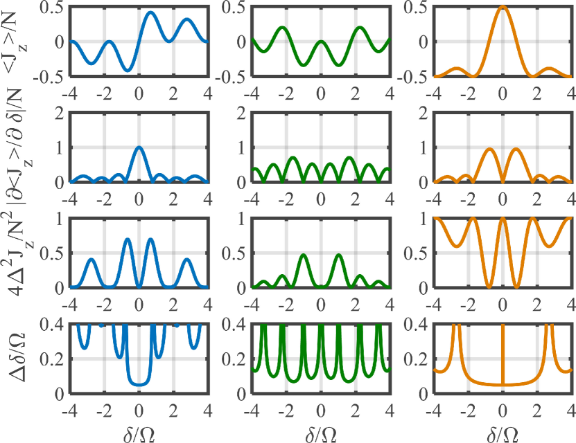
Figure S1: The first, second and third column represent the results with initial state $|\psi\rangle_{0}=|\pi/2,0\rangle_{SCS},|\pi/2,\pi/2\rangle_{SCS}$, and $|\pi,0\rangle_{SCS}$, respectively. The first, second, third and fourth row respectively correspond to the population difference, absolute slope of the population difference, variance of population difference and the measurement precision versus detuning. Here, atom number $N=100$, $\Omega T=\pi$.

Appendix B II. Measurement precisions for noninteracting systems

Below we show how to calculate measurement precisions for noninteracting systems (i.e. $\chi=0$). Given $\delta$ and $\Omega$, we first need to analytically obtain the expressions of $\langle\hat{J}_{z}^{2}(T)\rangle$. It is easy to find that $\langle\hat{J}_{z}^{2}(T)\rangle=\langle\psi(T)|\hat{J}_{z}^{2}|\psi(T)\rangle=_{0}\!\!\langle\psi|e^{i\hat{H}_{R}T}\hat{J_{z}^{2}}e^{-i\hat{H}_{R}T}|\psi\rangle_{0}=_{0}\!\!\langle\psi|e^{i\hat{H}_{R}T}\hat{J_{z}}e^{-i\hat{H}_{R}T}e^{i\hat{H}_{R}T}\hat{J_{z}}e^{-i\hat{H}_{R}T}|\psi\rangle_{0}$. Thus,

$$\langle\hat{J}_{z}^{2}(T)\rangle = {}_{0}\langle\psi|\left(X\hat{J}_{x}+Y\hat{J}_{y}+Z\hat{J}_{z}\right)^{2}|\psi\rangle_{0}$$ (S18)

$$= XX\langle\hat{J_{x}^{2}}\rangle_{0}+YY\langle\hat{J_{y}^{2}}\rangle_{0}+ZZ\langle\hat{J_{z}^{2}}\rangle_{0}$$

$$+ XY\langle\{\hat{J_{x}},\hat{J_{y}}\}\rangle_{0}+YZ\langle\{\hat{J_{y}},\hat{J_{z}}\}\rangle_{0}$$

$$+ XZ\langle\{\hat{J_{x}},\hat{J_{z}}\}\rangle_{0},$$

where $XX=X^{2}(\Omega,\delta,T)$, $YY=Y^{2}(\Omega,\delta,T)$, $ZZ=Z^{2}(\Omega,\delta,T)$, $XY=X(\Omega,\delta,T)Y(\Omega,\delta,T)$, $YZ=Y(\Omega,\delta,T)Z(\Omega,\delta,T)$, $XZ=X(\Omega,\delta,T)Z(\Omega,\delta,T)$, and $\{\star,\bullet\}=\star\bullet+\bullet\star$ denotes the anti-commutator. According to Eqs. (S17) and (S18), we can explicitly write the expression,

$$\Delta\hat{J}_{z}=\sqrt{\langle\hat{J}_{z}^{2}(T)\rangle-\langle\hat{J}_{z}(T)\rangle^{2}}.$$ (S19)

Besides, the deviation $\partial\langle\hat{J}_{z}(T)\rangle/\partial\delta$ can also be analytically obtained, which reads

$$\frac{\partial\langle\hat{J}_{z}(T)\rangle}{\partial\delta}=X^{\prime}\langle\hat{J_{x}}\rangle_{0}+Y^{\prime}\langle\hat{J_{y}}\rangle_{0}+Z^{\prime}\langle\hat{J_{z}}\rangle_{0},$$ (S20)

with

$$X^{\prime} = \frac{\Omega}{\Omega^{2}+\delta^{2}}\left[1-\cos(\sqrt{\Omega^{2}+\delta^{2}}T)\right]+\frac{\delta^{2}\Omega T}{(\Omega^{2}+\delta^{2})^{3/2}}\left[\sin(\sqrt{\Omega^{2}+\delta^{2}}T)\right]$$ (S21)

$$-\frac{2\delta^{2}\Omega}{(\Omega^{2}+\delta^{2})^{2}}\left[1-\cos(\sqrt{\Omega^{2}+\delta^{2}}T)\right],$$

$$Y^{\prime} = \frac{\delta\Omega T}{\Omega^{2}+\delta^{2}}\cos(\sqrt{\Omega^{2}+\delta^{2}}T)-\frac{\delta\Omega}{(\Omega^{2}+\delta^{2})^{3/2}}\sin(\sqrt{\Omega^{2}+\delta^{2}}T),$$ (S22)

$$Z^{\prime} = \frac{2\delta}{\Omega^{2}+\delta^{2}}+\frac{2\delta^{3}}{(\Omega^{2}+\delta^{2})^{2}}-\frac{\delta\Omega^{2}T}{(\Omega^{2}+\delta^{2})^{3/2}}\sin(\sqrt{\Omega^{2}+\delta^{2}}T)$$ (S23)

$$-\frac{2\delta\Omega^{2}}{(\Omega^{2}+\delta^{2})^{2}}\cos(\sqrt{\Omega^{2}+\delta^{2}}T).$$

Finally, according to Eqs. (S17) - (S25),

$$\Delta\delta=\frac{\Delta\hat{J}_{z}}{|\partial\langle\hat{J}_{z}(T)\rangle/\partial\delta|}$$ (S24)

can also be analytically expressed. Since $\delta=\omega_{0}-\omega$, the standard deviation $\Delta\omega_{0}=\Delta\delta$ mathematically. For convenience, we calculate the measurement precision $\Delta\omega_{0}$ by $\Delta\delta$ instead.

Appendix C III. Analytical analysis on antisymmetric locking signal for noninteracting systems

Below we analyze the antisymmetric locking signal for noninteracting systems. From Eqs. (S14) - (S17), one can easily find that $X(\Omega,\delta,T)=-X(\Omega,-\delta,T)$, $Y(\Omega,\delta,T)=Y(\Omega,-\delta,T)$ and $Z(\Omega,\delta,T)=Z(\Omega,-\delta,T)$ so that $\langle\hat{J}_{z}(\delta,T)\rangle=-\langle\hat{J}_{z}(-\delta,T)\rangle$ if $\langle\hat{J_{y}}\rangle_{0}=\langle\hat{J_{z}}\rangle_{0}=0$. For example, if the initial state is $|\psi\rangle_{0}=|\pi/2,0\rangle_{SCS}$, $\langle\hat{J_{x}}\rangle_{0}=\frac{N}{2}$ and $\langle\hat{J_{z}}\rangle_{0}=\langle\hat{J_{y}}\rangle_{0}=0$, the final population difference $\langle\hat{J}_{z}(T)\rangle$ is antisymmetric with $\delta=0$. While for $|\psi\rangle_{0}=|\pi/2,\pi/2\rangle_{SCS}$ and $|\psi\rangle_{0}=|\pi,0\rangle_{SCS}$ (both with $\langle\hat{J_{x}}\rangle_{0}=0$), the final population difference $\langle\hat{J}_{z}(T)\rangle$ is symmetric with $\delta=0$. The comparisons with these three different initial states are shown in the first row of Fig. S1.

From Eq. (S25), we can plot the absolute slope of population difference $|\partial\langle\hat{J}_{z}(T)\rangle/\partial\delta|$ versus detuning, see the second row of Fig. S1. There is a peak at $\delta=0$ for $|\psi\rangle_{0}=|\pi/2,0\rangle_{SCS}$, while the slope equals 0 for both $|\psi\rangle_{0}=|\pi/2,\pi/2\rangle_{SCS}$ and $|\psi\rangle_{0}=|\pi,0\rangle_{SCS}$.

From Eq. (S19), we can also plot the variance of population difference $\Delta^{2}\hat{J}_{z}$ versus detuning, see the third row of Fig. S1. Finally, according to Eq. (S24), we can analytically obtain the measurement precision $\Delta\delta$ versus detuning, see the last row of Fig. S1. It is obviously shown that, only $|\psi\rangle_{0}=|\pi/2,0\rangle_{SCS}$ can achieve high-precision measurement at the locking point $\delta=0$, while for $|\psi\rangle_{0}=|\pi/2,\pi/2\rangle_{SCS}$ and $|\psi\rangle_{0}=|\pi,0\rangle_{SCS}$, the measurement precisions are diverged.

The slope of the signal at the locking point $\delta=0$ can be analytically written as

$$\frac{\partial\langle\hat{J}_{z}(T)\rangle}{\partial\delta}|_{\delta=0}=\frac{N}{2}\frac{1-\cos\Omega T}{\Omega}.$$ (S25)

When $\Omega T=\pi$, $\frac{\partial\langle\hat{J}_{z}(T)\rangle}{\partial\delta}|_{\delta=0}=N/\Omega$ attains its maximum, which indicates the high sensitivity for frequency locking. At the locking point $\delta=0$, $\Delta\delta\propto 1/\sqrt{N}$, which exhibits the SQL scaling.

Appendix D IV. Analytical analysis on antisymmetric locking signal for interacting systems

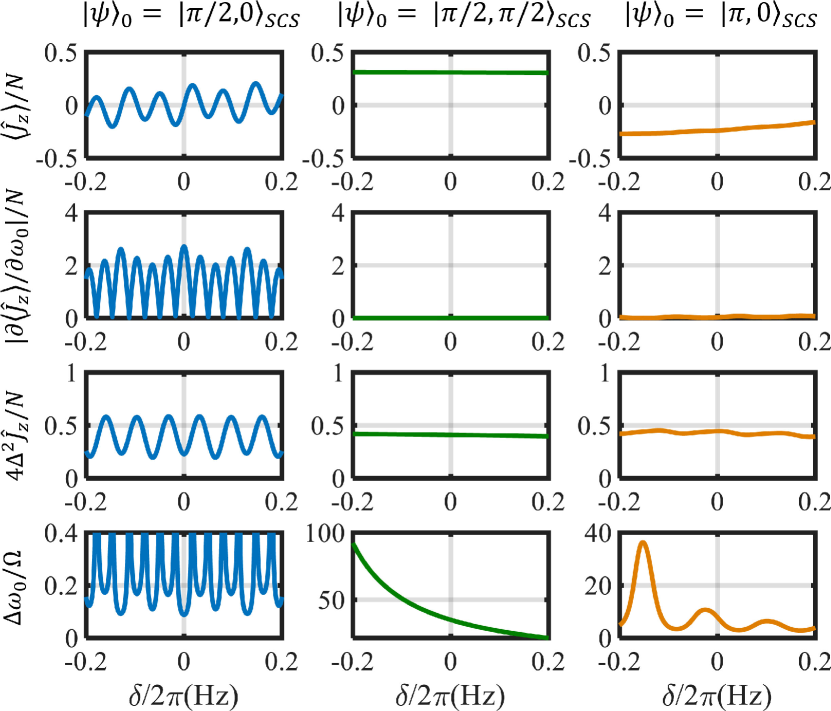
Figure S2: The first, second and third column represents the results with initial state $|\psi\rangle_{0}=|\pi/2,0\rangle_{SCS},|\pi/2,\pi/2\rangle_{SCS}$, and $|\pi,0\rangle_{SCS}$, respectively. The first, second, third and fourth row respectively correspond to the population difference, absolute slope of the population difference, variance of population difference and the measurement precision versus detuning. Here, atom number $N=100$, $\chi=2\pi\times 0.063$ Hz, $\Omega=2\pi\times 3.15$ Hz, and $T=0.198/\chi=0.5$ s.

In this section, we illustrate the mathematical analysis on the antisymmetric locking signal $\langle\hat{J}_{z}(\delta,T)\rangle$ (versus $\delta$) when atom-atom interaction is taken into account.

In the Schrodinger picture, the final state evolved from the initial state $|\psi\rangle_{0}$ at time $T$ can be calculated as

$$|\psi(T)\rangle_{f}=e^{i\hat{H}_{R}^{\prime}T}=e^{-i(\chi\hat{J}_{z}^{2}+\Omega\hat{J_{x}}+\delta\hat{J}_{z})T}|\psi\rangle_{0}.$$ (S26)

In order to analytically analyze the principle of Rabi spectroscopy in the presence of atom-atom interaction, we work in the interaction picture. In the reference of $\hat{H}_{0}=\chi\hat{J}_{z}^{2}+\delta\hat{J}_{z}$, we have the Hamiltonian

$$\hat{H}_{I} = e^{i\hat{H}_{0}t}\Omega\hat{J}_{x}e^{-i\hat{H}_{0}t}$$ (S27)

$$= \frac{\Omega}{2}e^{i(\chi\hat{J_{z}^{2}}+\delta\hat{J_{z}})t}\left(\hat{J}_{+}+\hat{J}_{-}\right)e^{-i(\chi\hat{J_{z}^{2}}+\delta\hat{J_{z}})t}$$

$$= \frac{\Omega}{2}\left(\hat{J}_{+}^{I}+\hat{J}_{-}^{I}\right),$$

where $\hat{J}_{\pm}^{I}=e^{i(\chi\hat{J_{z}^{2}}+\delta\hat{J_{z}})t}\hat{J}_{\pm}e^{-i(\chi\hat{J_{z}^{2}}+\delta\hat{J_{z}})t}$. Since $\frac{d}{dt}\hat{J}_{\pm}^{I}=i\left[\chi\hat{J_{z}^{2}}+\delta\hat{J_{z}},\hat{J}_{\pm}^{I}\right]$, $\left[\hat{J}_{z},\hat{J}_{\pm}\right]=\pm\hat{J}_{\pm}$, and $\left\{\hat{J}_{z},\hat{J}_{\pm}\right\}=\hat{J}_{\pm}\left(2\hat{J}_{z}\pm 1\right)$, we have

$$\frac{d}{dt}\hat{J}_{\pm}^{I} = i\left[\chi\hat{J_{z}^{2}}+\delta\hat{J_{z}},\hat{J}_{\pm}^{I}\right]$$ (S28)

$$= i\chi\left[\hat{J_{z}^{2}},\hat{J}_{\pm}^{I}\right]+i\delta\left[\hat{J_{z}},\hat{J}_{\pm}^{I}\right]$$

$$= \pm i\chi\left\{\hat{J}_{z},\hat{J}_{\pm}^{I}\right\}+i\delta\left[\hat{J_{z}},\hat{J}_{\pm}^{I}\right]$$

$$= \pm i\hat{J}_{\pm}^{I}\left[\chi\left(2\hat{J}_{z}\pm 1\right)+\delta\right].$$

Therefore, the rasing and lowering operators in the interaction picture can be given as

$$\hat{J}_{\pm}^{I}=\hat{J}_{\pm}e^{i\chi t}e^{\pm i(\delta t+2\chi t\hat{J}_{z})}.$$ (S29)

The state in interaction picture can be expanded in terms of Dicke basis, i.e.,

$$|\psi(t)\rangle^{I}=\sum_{m=-N/2}^{N/2}C_{m}^{I}(t)|J,m\rangle,$$ (S30)

where $|\psi(t)\rangle^{I}=e^{i\hat{H}_{0}t}|\psi(t)\rangle$ with $|\psi(t)\rangle=\sum_{m=-N/2}^{N/2}C_{m}(t)|J,m\rangle$ the evolved state in Schrodinger picture. Hence, $C_{m}^{I}(t)=e^{i(\chi m^{2}+\delta m)t}C_{m}(t)$ and $C_{m}^{I}(0)=C_{m}(0)$.

The time-evolution in interaction picture obeys

$$i\frac{d}{dt}|\psi(t)\rangle^{I}=\hat{H}_{I}|\psi(t)\rangle^{I}=\frac{\Omega}{2}\left(\hat{J}_{+}^{I}+\hat{J}_{-}^{I}\right)|\psi(t)\rangle^{I}.$$ (S31)

Owing to the relations $\hat{J}_{+}|J,m\rangle=\sqrt{(J-m)(J+m+1)}|J,m+1\rangle=\lambda_{m}^{+}|J,m+1\rangle$ and $\hat{J}_{-}|J,m\rangle=\sqrt{(J+m)(J-m+1)}|J,m-1\rangle=\lambda_{m}^{-}|J,m-1\rangle$, we can get the equations for the coefficients $C_{m}^{I}(t)$. For a given $C_{m}^{I}(t)$, the equation reads

$$i\dot{C}_{m}^{I}(t) = \frac{\Omega}{2}e^{i\chi t}\left[\lambda_{m-1}^{+}C_{m-1}^{I}(t)e^{i\delta t+2i\chi t(m-1)}+\lambda_{m+1}^{-}C_{m+1}^{I}(t)e^{-i\delta t-2i\chi t(m+1)}\right]$$ (S32)

$$= \frac{\Omega}{2}e^{-i\chi t}\left[\lambda_{m-1}^{+}C_{m-1}^{I}(t)e^{i\delta t+2i\chi tm}+\lambda_{m+1}^{-}C_{m+1}^{I}(t)e^{-i\delta t-2i\chi tm}\right].$$

Since $\lambda_{m}^{+}=\lambda_{-m}^{-}$, we also have

$$i\dot{C}_{-m}^{I}(t) = \frac{\Omega}{2}e^{-i\chi t}\left[\lambda_{-m-1}^{+}C_{-m-1}^{I}(t)e^{i\delta t-2i\chi tm}+\lambda_{-m+1}^{-}C_{-m+1}^{I}(t)e^{-i\delta t+2i\chi tm}\right]$$ (S33)

$$= \frac{\Omega}{2}e^{-i\chi t}\left[\lambda_{m-1}^{+}C_{-(m-1)}^{I}(t)e^{-i\delta t+2i\chi tm}+\lambda_{m+1}^{-}C_{-(m+1)}^{I}(t)e^{i\delta t-2i\chi tm}\right].$$

In the following, we verify the antisymmetry property of $\langle\hat{J}_{z}(T)\rangle$ versus $\delta=0$. For fixed $\Omega$ and $\chi$ at time $t$, ${C}_{m}^{I}(\delta,t)$ is dependent on $\delta$. According to Eqs. (S32) and (S33), we have

$$i\dot{C}_{m}^{I}(\delta,t) = \frac{\Omega}{2}e^{-i\chi t}\left[\lambda_{m-1}^{+}C_{m-1}^{I}(t)e^{i\delta t+2i\chi tm}+\lambda_{m+1}^{-}C_{m+1}^{I}(t)e^{-i\delta t-2i\chi tm}\right],$$ (S34)

$$i\dot{C}_{-m}^{I}(-\delta,t) = \frac{\Omega}{2}e^{-i\chi t}\left[\lambda_{m-1}^{+}C_{-(m-1)}^{I}(t)e^{i\delta t+2i\chi tm}+\lambda_{m+1}^{-}C_{-(m+1)}^{I}(t)e^{-i\delta t-2i\chi tm}\right].$$ (S35)

If the coefficients of the initial state $|\psi(0)\rangle=|\psi\rangle_{0}=\sum_{m=-N/2}^{N/2}C_{m}(0)|J,m\rangle$ satisfy the condition

$$C_{m}(0)=C_{-m}(0)$$ (S36)

for arbitrary $m$, we can immediately find that $\dot{C}_{m}^{I}(\delta,t)=\dot{C}_{-m}^{I}(-\delta,t)$ and therefore

$${C}_{m}^{I}(\delta,t)={C}_{-m}^{I}(-\delta,t).$$ (S37)

At time $T$, the final population difference

$$\langle\hat{J}_{z}(T)\rangle = {}^{I}\!\langle\psi(T)|\hat{J}_{z}^{I}|\psi(T)\rangle^{I}=^{I}\!\!\langle\psi(T)|\hat{J}_{z}|\psi(T)\rangle^{I}$$ (S38)

$$= \sum_{m=-J}^{J}m|C_{m}^{I}(T)|^{2}.$$

For $\delta$, $\langle\hat{J}_{z}(\delta,T)\rangle=\sum_{m=-J}^{J}m|C_{m}^{I}(\delta,T)|^{2}$. While for $-\delta$, $\langle\hat{J}_{z}(-\delta,T)\rangle=\sum_{m=-J}^{J}m|C_{m}^{I}(-\delta,T)|^{2}=\sum_{m=-J}^{J}-m|C_{-m}^{I}(-\delta,T)|^{2}=-\sum_{m=-J}^{J}m|C_{m}^{I}(\delta,T)|^{2}$. Thus, we finally prove that

$$\langle\hat{J}_{z}(\delta,T)\rangle=-\langle\hat{J}_{z}(-\delta,T)\rangle.$$ (S39)

We choose the initial state as $|\psi\rangle_{0}=|\pi/2,0\rangle_{SCS}=\sum_{m=-J}^{J}(\frac{1}{2})^{2J}\sqrt{\frac{(2J)!}{(J+m)!(J-m)!}}|J,m\rangle$ in the main text which satisfies the condition (S36), thus we always get the antisymmetric locking signal for arbitrary final time $T$. For comparison, we also show the population difference versus detuning with initial states $|\psi\rangle_{0}=|\pi/2,\pi/2\rangle_{SCS}$, and $|\pi,0\rangle_{SCS}$. For these two initial states, $C_{m}(0)$ does not always equal to $C_{-m}(0)$, thus the population difference is neither antisymmetric nor symmetric with respect to $\delta=0$, see the first row in Fig. S2. The absolute slope of the population difference, variance of population difference and the measurement precision versus detuning are also shown in the last three rows of Fig. S2.

Appendix E V. Realization of $\pi/2$ pulse for preparing the initial state

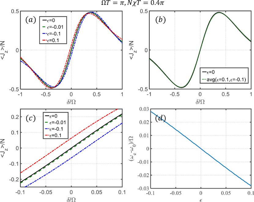
Figure S3: The locking signal versus detuning with imperfect $\pi/2$ pulse for $\Omega T=\pi$ and $N\chi T=0.4\pi$. The deviation to a perfect $\pi/2$ is characterized by $\epsilon$. (a) The scaled population difference versus detuning under different $\pi/2$ pulse with $\epsilon=0,-0.01,-0.1,0.1$. (b) The average signal $\frac{1}{2}(\langle\hat{J}_{z}(\delta,\epsilon)\rangle+\langle\hat{J}_{z}(\delta,-\epsilon)\rangle)$ with $\epsilon=0.1$, in comparison with the perfect signal. (c) The enlarged area of (a). (d) The shift of antisymmetric point versus deviation $\epsilon$. Here, we choose $N=100$, $\Omega=1$.

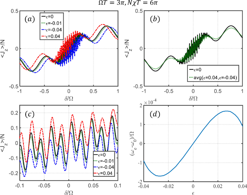
Figure S4: The locking signal versus detuning with imperfect $\pi/2$ pulse for $\Omega T=3\pi$ and $N\chi T=6\pi$. The deviation to a perfect $\pi/2$ is characterized by $\epsilon$. (a) The scaled population difference versus detuning under different $\pi/2$ pulse with $\epsilon=0,-0.01,-0.04,0.04$. (b) The average signal $\frac{1}{2}(\langle\hat{J}_{z}(\delta,\epsilon)\rangle+\langle\hat{J}_{z}(\delta,-\epsilon)\rangle)$ with $\epsilon=0.04$, in comparison with the perfect signal. (c) The enlarged area of (a). (d) The shift of antisymmetric point versus deviation $\epsilon$. Here, we choose $N=100$, $\Omega=1$.

To generate the input state $|\psi\rangle_{0}=|\pi/2,0\rangle_{SCS}$ for Rabi spectroscopy in our scheme, it is necessary to apply a $\pi/2$ pulse along $y$ axis onto the state of all atoms in $|\downarrow\rangle$. First, we consider the imperfect $\pi/2$ pulse without atom-atom interaction and detuning, which can be characterized by

$$e^{i(\frac{1+\epsilon}{2})\pi\hat{J}_{y}},$$ (S40)

where $\epsilon$ is the deviation from $\pi/2$. This kind of imperfection mainly comes from the imprecise control of pulse duration. To better compare with the results in the main text, here we choose $N=100$ for numerical simulation, see Fig. S3 and S4.

When $\epsilon=0$, it is a perfect $\pi/2$ pulse along $y$ axis. Thus, the results for $\epsilon=0$ are consistent with the previous ones. When $\epsilon\neq 0$, the signal of $\langle\hat{J}_{z}\rangle$ will deviate from the perfect one. In Fig. S3 (a) and (c), for $\Omega T=\pi$ and $\chi T=0.4\pi/N$, the signal deviation is not obvious even under $\epsilon=\pm 0.1$. We show the shift of antisymmetric point $\omega_{e}-\omega_{0}$ versus $\epsilon$ in Fig. S3 (d). Here, $\omega_{e}$ is the antisymmetric point using imperfect pulse with $\epsilon$ and $\omega_{0}$ is the exact antisymmetric point with perfect pulse. The shift is only $|\omega_{e}-\omega_{0}|\sim 0.03\Omega$ even with $\epsilon=\pm 0.1$. While for $\Omega T=3\pi$ and $\chi T=6\pi/N$, the signal deviation is still small when $\epsilon=\pm 0.04$, see Fig. S4 (a) and (c). The shift is only $|\omega_{e}-\omega_{0}|\sim 0.0002\Omega$ in the range of $\epsilon\in[-0.04,0.04]$, see Fig. S4 (d).

However, one can find that the deviations for $\pm\epsilon$ are antisymmetric with respect to $0$, i.e., $\langle\hat{J}_{z}(\delta,\epsilon)\rangle-\langle\hat{J}_{z}(\delta,\epsilon=0)\rangle=-(\langle\hat{J}_{z}(\delta,-\epsilon)\rangle-\langle\hat{J}_{z}(\delta,\epsilon=0)\rangle)$, as can be seen in Fig. S3 (d) and Fig. S4 (d). Therefore, the average signal $\frac{1}{2}(\langle\hat{J}_{z}(\delta,\epsilon)\rangle+\langle\hat{J}_{z}(\delta,-\epsilon)\rangle)$ becomes antisymmetric with respect to $\delta=0$, see Figs. S3 (b) and S4 (b). For nonzero $\chi$, the mean signal differs from the perfect one depending on $\epsilon$ and $\chi$. However, the antisymmetry will still possess. Thus in practice, one can scan the pulse duration to obtain the condition for perfect $\pi/2$ pulse ($\epsilon=0$) by analyzing the antisymmetry of the signal. The influences of the imperfect pulse can be easily eliminated in experiments.

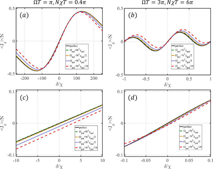
Figure S5: The final scaled half population difference $\langle\hat{J}_{z}\rangle/N$ versus detuning $\delta$ with different imperfect $\pi/2$ pulses. (a) $\Omega T=\pi$, $\chi T=0.4\pi/N$. (b) $\Omega T=3\pi$, $\chi T=6\pi/N$. (c) and (d) are the enlarged region (near on-resonance) of (a) and (b), respectively. Here, we choose $\chi=1$, $\chi_{pul}=\chi$, $N=100$. The black lines are the results with perfect $\pi/2$ pulse. Imperfect $\pi/2$ pulses are chosen with Rabi frequency $\Omega_{pul}=N^{2}\chi_{pul},N^{2}\chi_{pul}/2,N^{2}\chi_{pul}/5,N^{2}\chi_{pul}/10$ and pulse duration $t_{pul}=\frac{\pi}{2\Omega_{pul}}$.

In realistic experiments, even the duration of the pulse can be controlled precisely, the atom-atom interaction and the detuning may also affect the $\pi/2$ pulse. In the following, we take into account the atom-atom interaction and detuning when applying the $\pi/2$ pulse. The Hamiltonian for generating the $\pi/2$ pulse can be written as

$$H_{pul}=\chi_{pul}\hat{J}_{z}^{2}+\delta\hat{J}_{z}-\Omega_{pul}\hat{J}_{y},$$ (S41)

where $\chi_{pul}$ and $\Omega_{pul}$ denote the atom-atom interaction strength and the Rabi frequency during the pulse, respectively. Here, the detuning $\delta$ for $\pi/2$ pulse is the same as the one used in the following Rabi oscillation. Ideally, if no atom-atom interaction ($\chi_{pul}=0$) and on-resonant with $\delta=0$, a perfect input state can be prepared $|\pi/2,0\rangle_{SCS}=e^{i\frac{\pi}{2}\hat{J}_{y}}|\pi,0\rangle_{SCS}$ under the condition $\Omega_{pul}t_{pul}=\frac{\pi}{2}$ with $t_{pul}$ the duration of the pulse.

Taking into account $\chi_{pul}$ and $\delta$, the prepared state after the pulse can be expressed as

$$|\psi\rangle_{pul}=e^{-iH_{pul}t_{pul}}=e^{-i(\chi_{pul}\hat{J}_{z}^{2}+\delta\hat{J}_{z}-\Omega_{pul}\hat{J}_{y})t_{pul}}|\pi,0\rangle_{SCS}.$$ (S42)

Since

$$e^{-i(\chi_{pul}\hat{J}_{z}^{2}+\delta\hat{J}_{z}-\Omega_{pul}\hat{J}_{y})t_{pul}}=e^{-i(\chi_{pul}\hat{J}_{z}^{2}+\delta\hat{J}_{z})t_{pul}}e^{i\Omega_{pul}\hat{J}_{y})t_{pul}}e^{-\frac{\chi_{pul}\Omega_{pul}t_{pul}^{2}}{2}[\hat{J}_{z}^{2},\hat{J}_{y}]-\frac{\delta\Omega_{pul}t_{pul}^{2}}{2}[\hat{J}_{z},\hat{J}_{y}]}...,$$ (S43)

If $t_{pul}$ is sufficiently small, Eq. (S43) can be approximated as

$$e^{-i(\chi_{pul}\hat{J}_{z}^{2}+\delta\hat{J}_{z}-\Omega_{pul}\hat{J}_{y})t_{pul}}\approx e^{-i(\chi_{pul}\hat{J}_{z}^{2}+\delta\hat{J}_{z})t_{pul}}e^{i\Omega_{pul}\hat{J}_{y})t_{pul}}.$$ (S44)

Applying a $\pi/2$ pulse with $\Omega_{pul}t_{pul}=\frac{\pi}{2}$,

$$e^{-i(\chi_{pul}\hat{J}_{z}^{2}+\delta\hat{J}_{z}-\Omega_{pul}\hat{J}_{y})t_{pul}}\approx e^{-i\frac{\pi\chi_{pul}}{2\Omega_{pul}}\hat{J}_{z}^{2}-i\frac{\pi\delta}{2\Omega_{pul}}\hat{J}_{z}}e^{i\frac{\pi}{2}\hat{J}_{y}}.$$ (S45)

Since $e^{-i\frac{\pi\chi_{pul}}{2\Omega_{pul}}\hat{J}_{z}^{2}-i\frac{\pi\delta}{2\Omega_{pul}}\hat{J}_{z}}|\frac{N}{2},m\rangle=e^{-i\frac{\pi\chi_{pul}}{2\Omega_{pul}}m^{2}-i\frac{\pi\delta}{2\Omega_{pul}}m}|\frac{N}{2},m\rangle$, when $\frac{\pi\chi_{pul}}{2\Omega_{pul}}(\frac{N}{2})^{2}+\frac{\pi\delta}{2\Omega_{pul}}\frac{N}{2}\rightarrow 0$, $e^{-i\frac{\pi\chi_{pul}}{2\Omega_{pul}}\hat{J}_{z}^{2}-i\frac{\pi\delta}{2\Omega_{pul}}\hat{J}_{z}}|\frac{N}{2},m\rangle\approx\hat{I}|\frac{N}{2},m\rangle=|\frac{N}{2},m\rangle$ for all $m$. Therefore, the condition for realizing the $\pi/2$ pulse is

$$\Omega_{pul}\gg\frac{\pi N^{2}\chi_{pul}+2\pi\delta N}{8}.$$ (S46)

Thus the prepared state after applying $\pi/2$ pulse becomes

$$|\psi\rangle_{pul}=e^{-iH_{pul}t_{pul}}\approx e^{i\frac{\pi}{2}\hat{J}_{y}}|\pi,0\rangle_{SCS}=|\pi/2,0\rangle_{SCS},$$ (S47)

which is the desired SCS input state. If the $\pi/2$ pulse is perfect, the final signal $\langle\hat{J}_{z}(T)\rangle$ is exactly antisymmetric with detuning $\delta$ that can be used for determining the on-resonance frequency.

We find numerically that if the Rabi frequency

$$\Omega_{pul}\sim N^{2}\chi_{pul}/2,$$ (S48)

the $\pi/2$ pulse is nearly perfect and the antisymmetric spectrum can still be preserved. In Fig. S5, we show the final signal versus detuning using the input state prepared by $\pi/2$ pulse of different $\Omega_{pul}$. Here, we assume $\chi_{pul}=\chi=1$ for simulation. For both cases using $\Omega T=\pi,N\chi T=0.4\pi$ and $\Omega T=3\pi,N\chi T=6\pi$ for Rabi oscillation, the $\pi/2$ pulse satisfying Eq. (S46) can work well. When $\Omega_{pul}=N^{2}\chi_{pul}$, the obtained signal is nearly the same with the perfect one. As $\Omega_{pul}$ decreases, the signal begins to deviate and gradually becomes not antisymmetric with $\delta$. Despite the antisymmetry breaks down, the zero point $\langle\hat{J}_{z}(t)\rangle=0$ can still be used for frequency locking since the deviation is tiny, see the case of $\Omega_{pul}=0.1N^{2}\chi_{pul}$ in Fig. S5 (c) and (d).

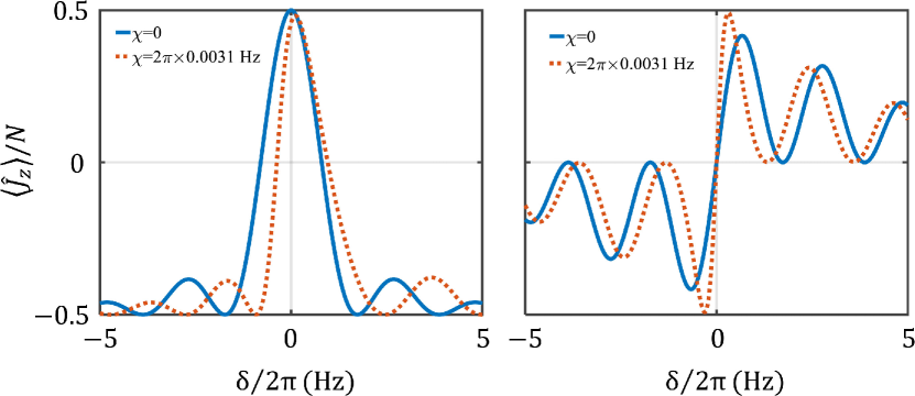
Figure S6: The conventional Rabi spectroscopy (left) and anti-symmetric Rabi spectroscopy (right) in the presence of atom-atom interaction. Here, the atom number $N=400$, Rabi frequency $\Omega=2\pi\times 1$ Hz and $T=0.5$ s. The blue (solid) and orange (dotted) lines are the results of $\chi=0$ and $\chi=2\pi\times 0.0031$ Hz.

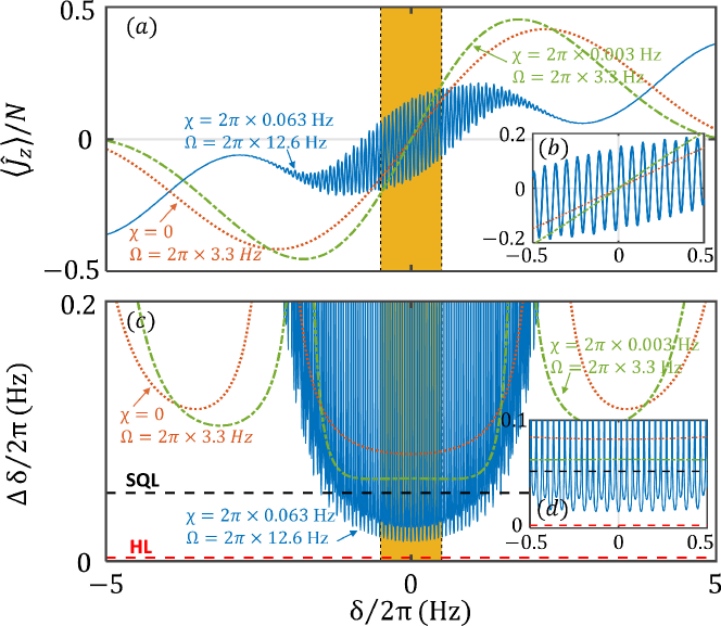
Figure S7: (a) The scaled population difference $\langle\hat{J}_{z}(T)\rangle/N$ versus the detuning $\delta$ and (c) the measurement precision $\Delta\omega_{0}$ versus $\delta$ for individual atoms ($\chi=0$) with $\Omega=2\pi\times 3.3$ Hz, $T=0.1516$ s satisfying the optimal condition $\Omega T=\pi$ and interacting atoms (strong atom-atom interaction $\chi=2\pi\times 0.0063$ Hz with $\Omega=2\pi\times 12.6$ Hz, $T=0.1516$ s ; background atom-atom interaction $\chi=2\pi\times 0.0003$ Hz with $\Omega=2\pi\times 3.3$ Hz, $T=0.1516$ s. (b) and (d) are the insets for the enlarged orange shaded region in (a) and (c), respectively. Here, the total atom number $N=400$ with a perfect initial state $|\psi\rangle_{0}=|\pi/2,0\rangle_{SCS}$.

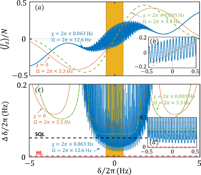
Figure S8: Simulation results with using imperfect $\pi/2$ pulse for input state preparation. Here, $\Omega_{pul}=2\pi\times 600$ Hz with $t_{pul}=0.416$ ms. The atom-atom interaction is the same during the whole spectroscopy $\chi_{pul}=\chi$. (a) The scaled population difference $\langle\hat{J}_{z}(T)\rangle/N$ versus the detuning $\delta$ and (c) the measurement precision $\Delta\omega_{0}$ versus $\delta$ for individual atoms ($\chi=0$) with $\Omega=2\pi\times 3.3$ Hz, $T=0.1516$ s satisfying the optimal condition $\Omega T=\pi$ and interacting atoms (strong atom-atom interaction $\chi=2\pi\times 0.0063$ Hz with $\Omega=2\pi\times 12.6$ Hz, $T=0.1516$ s ; background atom-atom interaction $\chi=2\pi\times 0.0003$ Hz with $\Omega=2\pi\times 3.3$ Hz, $T=0.1516$ s. (b) and (d) are the insets for the enlarged orange shaded region in (a) and (c), respectively. Here, the total atom number $N=400$.

Appendix F VI. Experimental feasibility via Bose condensed atoms

In the following, we take the system of Bose condensed atoms for an example [49]. Another example in collective cavity-QED system is shown in the next section. We compare the locking signals using our scheme with and without atom-atom interaction.

A Bose-Einstein condensate of ⁸⁷Rubidium has been considered as a promising candidate to create coherent spin squeezing based on two hyperfine states [49, 44, 58]. The $|F,m_{F}\rangle=|1,1\rangle$ and $|2,-1\rangle$ states in the lower and upper hyperfine manifold are suitable states for the high-precision measurement experiment. They fulfill the two major requirements: the tunability of interspecies interactions and their Zeeman energy shifts are to first order common mode with respect to magnetic fields.

The two states are coupled by a two-photon transition comprising of two frequencies in microwave regime and radio-frequency regime, respectively. The Rabi frequency strength is controlled by the intensity of the electromagnetic radiation. In the typical Bose condensed atomic system of ⁸⁷Rb with atom number $N=400$, for the chosen hyperfine states, the background effective scattering length (in the absence of magnetic field) is given as $a_{aa}+a_{bb}-2a_{ab}\approx 0.5a_{B}$ resulting in a nonlinearity $\chi\approx 2\pi\times 0.0031$ Hz. The Rabi frequency can be changed from 0 to $2\pi\times 600$ Hz.

F.1 A. Comparison between conventional and antisymmetric Rabi spectroscopy

For the conventional Rabi spectroscopy, to achieve better measurement precision, the Rabi frequency should be small. Here, we choose $\Omega=2\pi\times 1$ Hz with $T=0.5$ s for simulation. Considering the background atom-atom interaction, the spectrum has a small shift and the lineshape is no longer symmetric with $\delta=0$, see Fig. S6 (a). This collision shift is harmful for accurately determining the resonance frequency. In contrast, using the antisymmetric Rabi spectroscopy, the spectrum is always antisymmetric with $\delta=0$, see Fig. S6 (b). The resonance point will not alter when atom-atom interaction is taken into account. Other results for tunable atom-atom interaction are shown in Fig. 2 and Fig. 3 in the main text, in which the measurement precision can reach beyond SQL with suitably chosen atom-atom interaction $\chi$, Rabi frequency $\Omega$ and evolution time $T$.

F.2 B. Interaction-enhanced sensing via antisymmetric Rabi spectroscopy

We choose $\chi=2\pi\times 0.063$ Hz, which is a typical atom-atom interaction strength for one-axis twisting with the total atom number $N\approx 400$ in experiment [49, 59]. The Rabi frequency is chosen as $\Omega=N\chi/2=2\pi\times 12.6$ Hz, which is the optimal condition for twist-and-turn dynamics [60, 61, 62] whose Hamiltonian is similar to Eq. (3) in the main text. For $N=400$, we numerically find the optimal evolution time $T=0.06/\chi\approx 0.1516$ s. In comparison with the one via non-interacting atoms, we choose $T=0.1516$ s and $\Omega=2\pi\times 3.3$ Hz which satisfy the optimal condition $\Omega T=\pi$. Meanwhile, we also consider the case with background atom-atom interaction $\chi=2\pi\times 0.003$.

As shown in Fig. S7 (a) and (b), in the presence of background atom-atom interaction, the measurement precision can be improved compared to the non-interacting case. While with stronger atom-atom interaction and Rabi frequency ($\chi=2\pi\times 0.063$ and $\Omega=2\pi\times 12.6$), the locking signal with oscillates dramatically (especially near $\delta=0$). Unlike the conventional Rabi spectroscopy, the resolution of the antisymmetric Rabi spectroscopy can be greatly enhanced in the presence of atom-atom interaction. The slope at the on-resonance point is much sharper which indicates better sensitivity for frequency locking. In Fig. S7 (c) and (d), the measurement precisions are shown. Here, for the same evolution time $T$, the measurement precision with $\chi>0$ is much better than the ones with $\chi=0$. With optimized $\chi$ and $\Omega$, the measurement precision can surpass the SQL, $(\Delta\omega_{0})_{SQL}\propto 1/(\sqrt{N}T)$.

F.3 C. Influences of imperfect $\pi/2$ pulse for preparing the initial state

To obtain the desired input state for antisymmetric Rabi spectroscopy, one needs to use a short $\pi/2$ pulse with large Rabi frequency $\Omega_{pul}$. In this experimental system, the Rabi frequency can be up to $\Omega_{pul}=2\pi\times 600$ Hz. For small atom-atom interaction $\chi=2\pi\times 0.003$ Hz, $\Omega_{pul}=2\pi\times 600$ Hz is much larger than $N^{2}\chi$, which satisfies the condition (S46), see the dashed line in Fig. S8 (a) and (b). Thus, the signal is exactly antisymmetric with $\delta$ and the measurement precision is the same with the perfect one, see the dashed lines in Fig. S8 (c) and (d). For strong atom-atom interaction $\chi=2\pi\times 0.063$ Hz, despite the Rabi frequency $\Omega_{pul}=2\pi\times 600$ Hz does not meet the strong Rabi frequency condition (S46), we find that it is sufficient to observe the antisymmetric signal and the shift of the antisymmetric point is small. As shown in Fig. S8 (a), the blue solid line becomes not exactly antisymmetric with respect to detuning. Looking closer in the vicinity of the on-resonance point, there appears a shift compared to the perfect one. However, this shift is extremely small, which merely affect the accuracy of determining the on-resonance frequency. Besides, the measurement precision hardly change compared to the perfect one. Thus, the antisymmetric Rabi spectroscopy is experimentally feasible with state-of-the-art techniques via Bose condensed atoms.

Appendix G VII. Experimental feasibility via collective Cavity-QED system

Figure S9: (a) The final population difference at time $T$ versus $\delta$ and (b) the measurement precision versus $T$ at $\delta=0$ with individual atoms ($\chi=0$) and interacting atoms ($\chi=2\pi\times 10$ Hz). For $\chi=2\pi\times 10$ Hz, we choose $\Omega=2\pi\times 3500$ Hz, $T=0.636$ ms. For $\chi=0$, we choose $\Omega=2\pi\times 785$ Hz, $T=0.636$ ms under the optimal condition $\Omega T=\pi$. (c) is the enlarged orange shaded region in (b).(d) The final population difference at time $T$ versus $\delta$ and (e) the measurement precision versus $T$ at $\delta=0$ using our scheme and Ramsey scheme with spin squeezed state generated via one-axis twisting. For the latter scheme, we consider optimal squeezing with $T_{p}=3^{1/6}N^{-2/3}/\chi$ and the Ramsey interrogation time $T_{R}=T-T_{p}$. For both schemes, $\chi=2\pi\times 10$ Hz, $T=0.636$ ms. (f) is the enlarged orange shaded region in (e). Here, atom number $N=700$.

Our scheme can also be applied to other many-body quantum systems, such as the collective cavity-QED system. For the atomic ensemble in an optical cavity [54, 53, 55], the one-axis twisting can be generated by quantum non-demolition measurements and cavity-mediated spin interaction. In Ref. [56], the spin squeezed states created by quantum non-demolition measurements and cavity-mediated spin interaction are demonstrated, which provides an ideal platform for achieving the quantum enhanced measurement via antisymmetric Rabi spectroscopy.

In this kind of experimental systems, the interaction strength $\chi$ can be easily tuned via tuning the detuning of the probe laser. Thus, for the input state preparation stage, one can use a small $\chi_{pul}$ to achieve a perfect $\pi/2$ pulse with $\Omega_{pul}\gg N^{2}\chi_{pul}$. Then, one can use a large $\chi$ for implementing the Rabi oscillations to realize the interaction-enhanced sensing via antisymmetric Rabi spectroscopy.

In the experiment [56], the one-axis twisting strength can be up to $\chi_{OAT}\approx 2\pi\times 10$ Hz with atom number $N\approx 700$. Thus, in our simulation for implementing Rabi oscillations, we choose $\chi=2\pi\times 10$ Hz and $N=700$. With Rabi frequency $\Omega=N\chi/2=2\pi\times 3500$ Hz, the optimal evolution time can be numerically obtained as $T=0.636$ ms. Under the same evolution time, we choose $\Omega=2\pi\times 785$ Hz in the case of $\chi=0$ for comparison. Besides, we also compare the results of using Ramsey spectroscopy with optimal one-axis twisting spin squeezed state. The results are shown in Fig. S9, which are similar with the ones in Bose condensed atomic system. According to these results, our protocol can also greatly improves the resolution of the spectrum and the frequency measurement precision in the collective cavity-QED systems.

References

• Degen et al. [2017] C. L. Degen, F. Reinhard,  and P. Cappellaro, “Quantum sensing,” Rev. Mod. Phys. 89, 035002 (2017).
• Kitching et al. [2011] John Kitching, Svenja Knappe,  and Elizabeth A. Donley, “Atomic sensors – a review,” IEEE Sensors Journal 11, 1749–1758 (2011).
• Diddams et al. [2004] S. A. Diddams, J. C. Bergquist, S. R. Jefferts,  and C. W. Oates, “Standards of Time and Frequency at the Outset of the 21st Century,” Science 306, 1318–1324 (2004).
• Oelker et al. [2019] E. Oelker, R. B. Hutson, C. J. Kennedy, L. Sonderhouse, T. Bothwell, A. Goban, D. Kedar, C. Sanner, J. M. Robinson, G. E. Marti, D. G. Matei, T. Legero, M. Giunta, R. Holzwarth, F. Riehle, U. Sterr,  and J. Ye, “Demonstration of 4.8 x 10⁻¹⁷ stability at 1 s for two independent optical clocks,” Nature Photonics 13, 714–719 (2019).
• Orenes et al. [2021] Daniel Benedicto Orenes, Robert J. Sewell, Jérôme Lodewyck,  and Morgan W. Mitchell, “Improving Short-Term Stability in Optical Lattice Clocks by Quantum Nondemolition Measurements,” Phys. Rev. Lett. 128, 153201 (2021).
• Baumgart et al. [2016] I. Baumgart, J.-M. Cai, A. Retzker, M. B. Plenio,  and Ch Wunderlich, “Ultrasensitive Magnetometer using a Single Atom,” Phys. Rev. Lett. 116, 240801 (2016).
• Smullin et al. [2009] S. J. Smullin, I. M. Savukov, G. Vasilakis, R. K. Ghosh,  and M. V. Romalis, “Low-noise high-density alkali-metal scalar magnetometer,” Phys. Rev. A 80, 033420 (2009).
• Shi et al. [2018] Hao Shi, Ma Jie, Xiaofeng Li, Jie Liu, Chao Li,  and Shougang Zhang, “A quantum-based microwave magnetic field sensor,” Sensors 18, 3288 (2018).
• Simpson et al. [1963] J. H. Simpson, J. T. Fraser,  and I. A. Greenwood, “An optically pumped nuclear magnetic resonance gyroscope,” IEEE Transactions on Aerospace 1, 1107–1110 (1963).
• Szigeti et al. [2021] Stuart S Szigeti, Onur Hosten,  and Simon A. Haine, “Improving cold-atom sensors with quantum entanglement: Prospects and challenges,” Applied Physics Letters 118, 140501 (2021).
• Giovannetti et al. [2006] Vittorio Giovannetti, Seth Lloyd,  and Lorenzo Maccone, “Quantum metrology,” Phys. Rev. Lett. 96, 010401 (2006).
• Lee [2006] Chaohong Lee, “Adiabatic mach-zehnder interferometry on a quantized bose-josephson junction,” Phys. Rev. Lett. 97, 150402 (2006).
• Huang et al. [2014] Jiahao Huang, Shuyuan Wu, Honghua Zhong,  and Chaohong Lee, Quantum Metrology with Cold Atoms, Vol. 2 (2014) pp. 365–415.
• Pezzè et al. [2018] Luca Pezzè, Augusto Smerzi, Markus K. Oberthaler, Roman Schmied,  and Philipp Treutlein, “Quantum metrology with nonclassical states of atomic ensembles,” Rev. Mod. Phys. 90, 035005 (2018).
• Lu et al. [2019] Bo Lu, Cheng-Yin Han, Min Zhuang, Yong-Guan Ke, Jia-Hao Huang,  and Chao-Hong Lee, “Non-gaussian entangled states and quantum metrology with ultracold atomic ensemble,” Acta Physica Sinica 68, 040306 (2019).
• Rabi et al. [1938] I I Rabi, S Millman, P Kusch,  and J R Zacharias, “The molecular beam resonance method for measuring nuclear magnetic moments,” Phys. Rev 53, 318 (1938).
• Ramsey [1949] Norman F. Ramsey, “A new molecular beam resonance method,” Physical Review 76, 996–996 (1949).
• Ramsey [1950] Norman F. Ramsey, “A molecular beam resonance method with separated oscillating fields,” Physical Review 78, 695–699 (1950).
• Ramsey [1980] Norman F. Ramsey, “The method of successive oscillatory fields,” Physics Today 33, 25–30 (1980).
• Ludlow et al. [2015] Andrew D Ludlow, Martin M Boyd, Jun Ye, Ekkehard Peik,  and P. O. Schmidt, “Optical atomic clocks,” Rev. Mod. Phys. 87, 637–701 (2015).
• Kokkelmans et al. [1997] S. J. J. M. F. Kokkelmans, B. J. Verhaar, K. Gibble,  and D. J. Heinzen, “Predictions for laser-cooled rb clocks,” Phys. Rev. A 56, R4389–R4392 (1997).
• Szymaniec et al. [2007] K. Szymaniec, W. Chałupczak, E. Tiesinga, C. J. Williams, S. Weyers,  and R. Wynands, “Cancellation of the Collisional Frequency Shift in Caesium Fountain Clocks,” Phys. Rev. Lett. 98, 153002 (2007).
• Yu and Pethick [2010] Zhenhua Yu and C. J. Pethick, “Clock shifts of optical transitions in ultracold atomic gases,” Phys. Rev. Lett. 104, 010801 (2010).
• Lee et al. [2016] Sangkyung Lee, Chang Yong Park, Won Kyu Lee,  and Dai Hyuk Yu, “Cancellation of collisional frequency shifts in optical lattice clocks with Rabi spectroscopy,” New Journal of Physics 18 (2016).
• Shaniv et al. [2018] Ravid Shaniv, Tom Manovitz, Yotam Shapira, Nitzan Akerman,  and Roee Ozeri, “Toward heisenberg-limited rabi spectroscopy,” Phys. Rev. Lett. 120, 243603 (2018).
• [26] See Supplemental Material for details on: (i) Derivation of the half population difference Eq. (4), (ii) Measurement precisions for noninteracting systems, (iii) Analytical analysis on antisymmetric locking signal for noninteracting systems, (iv) Analytical analysis on antisymmetric locking signal for interacting systems, (v) Influences of imperfect $\pi/2$ pulse for preparing the initial state, (vi) Experimental feasibility via Bose condensed atoms, and (vii) Experimental feasibility via collective Cavity-QED system.
• Sanner et al. [2018] Christian Sanner, Nils Huntemann, Richard Lange, Christian Tamm,  and Ekkehard Peik, “Autobalanced ramsey spectroscopy,” Phys. Rev. Lett. 120, 53602 (2018).
• Lee [2009] Chaohong Lee, “Universality and anomalous mean-field breakdown of symmetry-breaking transitions in a coupled two-component bose-einstein condensate,” Phys. Rev. Lett. 102, 070401 (2009).
• Trenkwalder et al. [2016] A. Trenkwalder, G. Spagnolli, G. Semeghini, S. Coop, M. Landini, P. Castilho, L. Pezzè, G. Modugno, M. Inguscio, A. Smerzi,  and M. Fattori, “Quantum phase transitions with parity-symmetry breaking and hysteresis,” Nature Physics 12, 826–829 (2016).
• Zhuang et al. [2020] Min Zhuang, Jiahao Huang, Yongguan Ke,  and Chaohong Lee, “Symmetry-protected quantum adiabatic evolution in spontaneous symmetry-breaking transitions,” Annalen der Physik 532, 1900471 (2020).
• Takamoto et al. [2005] Masao Takamoto, Feng-Lei Hong, Ryoichi Higashi,  and Hidetoshi Katori, “An optical lattice clock,” Nature 435, 321–324 (2005).
• Norcia et al. [2019] Matthew A. Norcia, Aaron W. Young, William J. Eckner, Eric Oelker, Jun Ye,  and Adam M. Kaufman, “Seconds-scale coherence on an optical clock transition in a tweezer array,” Science 366, 93–97 (2019).
• Yin et al. [2022] Mo-Juan Yin, Xiao-Tong Lu, Ting Li, Jing-Jing Xia, Tao Wang, Xue-Feng Zhang,  and Hong Chang, “Floquet engineering hz-level rabi spectra in shallow optical lattice clock,” Phys. Rev. Lett. 128, 073603 (2022).
• Liu et al. [2017] Hui Liu, Xi Zhang, Kun-Liang Jiang, Jin-Qi Wang, Qiang Zhu, Zhuan-Xian Xiong, Ling-Xiang He,  and Bao-Long Lyu, “Realization of closed-loop operation of optical lattice clock based on 171yb*,” Chinese Physics Letters 34, 020601 (2017).
• Luo et al. [2020] Limeng Luo, Hao Qiao, Di Ai, Min Zhou, Shuang Zhang, Sheng Zhang, Changyue Sun, Qichao Qi, Chengquan Peng, Taoyun Jin, Wei Fang, Zhiqiang Yang, Tianchu Li, Kun Liang,  and Xinye Xu, “Absolute frequency measurement of an yb optical clock at the 10-16 level using international atomic time,” Metrologia 57, 065017 (2020).
• Nolan et al. [2017] Samuel P. Nolan, Stuart S. Szigeti,  and Simon A. Haine, “Optimal and robust quantum metrology using interaction-based readouts,” Phys. Rev. Lett. 119, 193601 (2017).
• Haine [2018] Simon A. Haine, “Using interaction-based readouts to approach the ultimate limit of detection-noise robustness for quantum-enhanced metrology in collective spin systems,” Phys. Rev. A 98, 030303 (2018).
• Huang et al. [2018a] Jiahao Huang, Min Zhuang,  and Chaohong Lee, “Non-gaussian precision metrology via driving through quantum phase transitions,” Phys. Rev. A 97, 032116 (2018a).
• Wineland et al. [1992] D. J. Wineland, J. J. Bollinger, W. M. Itano, F. L. Moore,  and D. J. Heinzen, “Spin squeezing and reduced quantum noise in spectroscopy,” Phys. Rev. A 46, R6797–R6800 (1992).
• Wineland et al. [1994] D. J. Wineland, J. J. Bollinger, W. M. Itano,  and D. J. Heinzen, “Squeezed atomic states and projection noise in spectroscopy,” Phys. Rev. A 50, 67–88 (1994).
• Louchet-Chauvet et al. [2010] Anne Louchet-Chauvet, Jürgen Appel, Jelmer J. Renema, Daniel Oblak, Niels Kjaergaard,  and Eugene S. Polzik, “Entanglement-assisted atomic clock beyond the projection noise limit,” New Journal of Physics 12, 065032 (2010).
• Kitagawa and Ueda [1993] Masahiro Kitagawa and Masahito Ueda, “Squeezed spin states,” Phys. Rev. A 47, 5138–5143 (1993).
• Ma et al. [2011] Jian Ma, Xiaoguang Wang, C.P. Sun,  and Franco Nori, “Quantum spin squeezing,” Physics Reports 509, 89–165 (2011).
• Gross [2012] Christian Gross, “Spin squeezing, entanglement and quantum metrology with bose-einstein condensates,” Journal of Physics B 45, 103001 (2012).
• Davis et al. [2016] Emily Davis, Gregory Bentsen,  and Monika Schleier-Smith, “Approaching the heisenberg limit without single-particle detection,” Phys. Rev. Lett. 116, 053601 (2016).
• Huang et al. [2018b] Jiahao Huang, Min Zhuang, Bo Lu, Yongguan Ke,  and Chaohong Lee, “Achieving heisenberg-limited metrology with spin cat states via interaction-based readout,” Phys. Rev. A 98, 012129 (2018b).
• Hosten et al. [2016] Onur Hosten, Nils J. Engelsen, Rajiv Krishnakumar,  and Mark A. Kasevich, “Measurement noise 100 times lower than the quantum-projection limit using entangled atoms,” Nature 529, 505–508 (2016).
• Li et al. [2021] Jinyang Li, Gregório R. M. da Silva, Schuyler Kain, Gour Pati, Renu Tripathi,  and Selim M. Shahriar, “Spin Squeezing Induced Enhancement of Sensitivity of an Atomic Clock using Coherent Population Trapping,”   (2021)arXiv:2112.08013 .
• Gross et al. [2010] C. Gross, T. Zibold, E. Nicklas, J. Estève,  and M. K. Oberthaler, “Nonlinear atom interferometer surpasses classical precision limit,” Nature 464, 1165–1169 (2010).
• Riedel et al. [2010] Max F. Riedel, Pascal Böhi, Yun Li, Theodor W. Hänsch Signnsch, Alice Sinatra,  and Philipp Treutlein, “Atom-chip-based generation of entanglement for quantum metrology,” Nature 464, 1170–1173 (2010).
• Ockeloen et al. [2013] Caspar F. Ockeloen, Roman Schmied, Max F. Riedel,  and Philipp Treutlein, “Quantum metrology with a scanning probe atom interferometer,” Phys. Rev. Lett. 111, 143001 (2013).
• Strobel et al. [2014] Helmut Strobel, Wolfgang Muessel, Daniel Linnemann, Tilman Zibold, David B. Hume, L. Pezze, Augusto Smerzi,  and Markus K. Oberthaler, “Fisher information and entanglement of non-gaussian spin states,” Science 345, 424–427 (2014).
• Colombo et al. [2022] Simone Colombo, Edwin Pedrozo-Peñafiel, Albert F. Adiyatullin, Zeyang Li, Enrique Mendez, Chi Shu,  and Vladan Vuletić, “Time-reversal-based quantum metrology with many-body entangled states,” Nature Physics  (2022), 10.1038/s41567-022-01653-5.
• Pedrozo-Peñafiel et al. [2020] Edwin Pedrozo-Peñafiel, Simone Colombo, Chi Shu, Albert F. Adiyatullin, Zeyang Li, Enrique Mendez, Boris Braverman, Akio Kawasaki, Daisuke Akamatsu, Yanhong Xiao,  and Vladan Vuletić, “Entanglement on an optical atomic-clock transition,” Nature 588, 414–418 (2020).
• Li et al. [2022] Zeyang Li, Boris Braverman, Simone Colombo, Chi Shu, Akio Kawasaki, Albert F. Adiyatullin, Edwin Pedrozo-Peñafiel, Enrique Mendez,  and Vladan Vuletić, “Collective spin-light and light-mediated spin-spin interactions in an optical cavity,” PRX Quantum 3, 020308 (2022).
• Greve et al. [2022] Graham P Greve, Chengyi Luo, Baochen Wu,  and James K Thompson, “Entanglement-enhanced matter-wave interferometry in a high-finesse cavity,” Nature 610, 472–477 (2022).
• Gilmore et al. [2021] Kevin A. Gilmore, Matthew Affolter, Robert J. Lewis-Swan, Diego Barberena, Elena Jordan, Ana Maria Rey,  and John J. Bollinger, “Quantum-enhanced sensing of displacements and electric fields with two-dimensional trapped-ion crystals,” Science 373, 673–678 (2021).
• Gross [2010] Christian Gross, “Spin squeezing and non-linear atom interferometry with bose-einstein condensates,” PhD dissertation  (2010).
• Juliá-Díaz et al. [2012] B. Juliá-Díaz, E. Torrontegui, J. Martorell, J. G. Muga,  and A. Polls, “Fast generation of spin-squeezed states in bosonic josephson junctions,” Phys. Rev. A 86, 063623 (2012).
• Muessel et al. [2015] W. Muessel, H. Strobel, D. Linnemann, T. Zibold, B. Juliá-Díaz,  and M. K. Oberthaler, “Twist-and-turn spin squeezing in bose-einstein condensates,” Phys. Rev. A 92, 023603 (2015).
• Mirkhalaf et al. [2018] Safoura S. Mirkhalaf, Samuel P. Nolan,  and Simon A. Haine, “Robustifying twist-and-turn entanglement with interaction-based readout,” Phys. Rev. A 97, 053618 (2018).
• Sorelli et al. [2019] Giacomo Sorelli, Manuel Gessner, Augusto Smerzi,  and Luca Pezzè, “Fast and optimal generation of entanglement in bosonic josephson junctions,” Phys. Rev. A 99, 022329 (2019).