Dynamics of a massive superfluid vortex in $r^{k}$ confining potentials

Abstract

We study the motion of a superfluid vortex in condensates having different background density profiles, ranging from parabolic to uniform. The resulting effective point-vortex model for a generic power-law potential $\propto r^{k}$ can be experimentally realized with recent advances in optical-trapping techniques. Our analysis encompasses both empty-core and filled-core vortices. In the latter case, the vortex acquires a mass due to the presence of distinguishable atoms located in its core. The axisymmetry allows us to reduce the coupled dynamical equations of motion to a single radial equation with an effective potential $V_{\rm eff}$. In many cases, $V_{\rm eff}$ has a single minimum, where the vortex precesses uniformly. The dynamics of the vortex and the localized massive core arises from the dependence of the energy on the radial position of the vortex and from the $r^{k}$ trap potential. We find that a positive vortex with small mass orbits in the positive direction, but the sense of precession can reverse as the core mass increases. Early experiments and theoretical studies on two-component vortices found some qualitatively similar behavior.

I Introduction

Superfluid vortices have been of great interest ever since Feynman’s seminal article in 1955 Feynman (1955). The creation of ultracold atomic Bose-Einstein condensates (BECs) in 1995 Pethick and Smith (2008); Pitaevskii and Stringari (2016) broadened the original focus on liquid ⁴He to include many new possibilities. The first BEC vortex was in a two-component condensate with two trapped hyperfine states of ⁸⁷Rb Matthews et al. (1999); Anderson et al. (2000), although most subsequent experiments Madison et al. (2000); Raman et al. (2001); Leanhardt et al. (2002); Scherer et al. (2007); Kwon et al. (2016) studied simpler one-component BECs.

In these mixtures, each component had its own resonant frequency and could be imaged separately, allowing nondestructive visualization of the large filled core, whose radius was larger than the optical resolution of the imaging system. Consequently, it was feasible to study the precession of two-component vortices in real time Anderson et al. (2000). In contrast, the empty core of a one-component vortex typically has a radius smaller than the wavelength of the imaging light and is observable only after free expansion by turning off the trap. Various methods subsequently allowed direct real-time observation of precession of a one-component vortex, the most direct visualizing the dynamics through expansion of successive small fractions of the condensate Freilich et al. (2010); Serafini et al. (2017). Collisions between vortices have also been studied in great detail Kwon et al. (2021); Richaud et al. (2022). Soon after the first experiments, theoretical studies used a time-dependent variational Lagrangian to study the precession of one-component and two-component vortices Lundh and Ao (2000); McGee and Holland (2001), although little detailed comparison was made with the experiments.

Various theoretical works have studied the dynamics of massive vortices over the last few years Richaud et al. (2020); Griffin et al. (2020); Richaud et al. (2021); Ruban (2022); Doran et al. (2022). In these systems, the vortex in component $a$ surrounds a localized massive core in component $b$, assuming interaction constants that would strongly favor phase separation of the two components in a uniform system. Our previous works focused on motion in a two-dimensional flat trap with a circular boundary Richaud et al. (2020, 2021). Here we extend our model to include a trap with a power-law potential $r^{k}$. For simplicity, we study a single vortex in a Thomas-Fermi condensate $a$. This model allows us to interpolate between the usual harmonic trap with $k=2$ and the flat trap Navon et al. (2021); Zou et al. (2021) in the limit $k\to\infty$.

The precession of an off-center vortex around the axis of an harmonic trap requires a non-trivial theoretical description (see Ref. Groszek et al. (2018) and references therein) due to the spatially-varying condensate’s density profile. Several works over the past twenty years considered models which included different features, like image vortices and core sizes that depend on the local density Jackson et al. (1999); Lundh and Ao (2000); Svidzinsky and Fetter (2000a, b); Kim and Fetter (2004); McGee and Holland (2001); Anglin (2002); Sheehy and Radzihovsky (2004); Jezek and Cataldo (2008); dos Santos (2016); Esposito et al. (2017); Biasi et al. (2017). Our model incorporates both features. For small $k$ (especially the harmonic trap with $k=2$), we find that the vortex precession rate can decrease and even reverse direction as the localized core mass increases. It is notable that earlier experimental and theoretical studies Anderson et al. (2000); McGee and Holland (2001) each found evidence of such reversal of precession, even though these studies were near the onset of bulk phase separation.

In our previous study of a single vortex in a flat potential with a circular boundary (see Sec. II.A of Ref. Richaud et al. (2021)), the Lagrangian for a vortex with a massive localized core had a term linear in the vortex velocity along with the usual kinetic energy that is quadratic in the vortex velocity. This linear term is familiar from the Lagrangian of a massive point particle in an external electromagnetic field. For this system in a flat trap, there is an effective uniform magnetic field $\bm{B}=-2\pi n_{a}\hbar\hat{\bm{z}}$, where $n_{a}$ is the two-dimensional number density of the background component. Our present analysis includes a nonuniform $r^{k}$ trapping potential, and the effective magnetic field also becomes nonuniform. More importantly, the corresponding effective vector potential $\bm{A}$ now appears in the Hamiltonian as a synthetic gauge field that depends explicitly on the choice of trap potential. This formulation generalizes the familiar Hamiltonian for massless vortices (see, for example Sec. 157 of Ref. Lamb (1945)).

The paper is structured as follows: Section II relies on the Thomas-Fermi model in a power-law trap to find the condensate density for a single-component BEC. This result allows us to obtain a time-dependent variational Lagrangian, based on a trial function describing a single quantized vortex in a power-law potential, along with its opposite-sign image outside the condensate. The Lagrangian characterizes the dynamics of a single vortex, which here yields uniform circular precession. Section III adds the massive localized core to obtain the Lagrangian for a massive point vortex. In addition to the usual kinetic energy of the core mass, it also has a term linear in the vortex velocity. We discuss the analogy with the electromagnetic Lagrangian for a charged particle and find the associated synthetic vector potential and synthetic magnetic field. The dynamics of a single massive point vortex typically involves uniform circular precession along with small stable oscillations around the local minimum in the effective potential. In some cases, however, this minimum disappears, and the vortex moves to the outer boundary. Positive massless vortices precess in the positive direction around the trap center, but we find that as their mass increases the precession frequency can reverse sign. We end with conclusions and outlook in Sec. IV.

II Thomas-Fermi model for single-component BEC

A single-component BEC is described, at the mean-field level, by the familiar Gross-Pitaevskii (GP) model

$$i\hbar\frac{\partial\Psi_{a}}{\partial t}=\!\!\left(\!-\frac{\hbar^{2}\nabla^{2}}{2m_{a}}+V_{\rm tr}+g_{aa}|\Psi_{a}|^{2}\!\right)\Psi_{a},$$ (1)

where $g_{aa}=2\sqrt{2\pi}\hbar^{2}a_{aa}/(m_{a}d_{z})$ represents the effective interaction in the quasi-2D system, $a_{aa}$ being the component-$a$ s-wave scattering length, $m_{a}$ its atomic mass, and $d_{z}$ the harmonic-oscillator length along the $z$-direction Hadzibabic and Dalibard (2011). Our analysis thus focuses on an effective 2D system (lying on the $xy$ plane), as the possible degrees of freedom along the $z$-axis are assumed to be frozen due to the strong confinement along that direction.

In the strongly-interacting Thomas-Fermi (TF) regime, for any axisymmetric potential $V_{\rm tr}(r)$, the TF condensate density $n_{a}(r)$ satisfies

$$\mu_{a}=V_{\rm tr}(r)+g_{aa}n_{a}(r).$$ (2)

Here $\mu_{a}=g_{aa}n_{0}$ is the chemical potential of the $a$ component, and $n_{0}=n_{a}(0)$ is the density at the center of the trap. If $n_{a}(r)$ vanishes at the TF radius $R$, then Eq. (2) implies that $g_{aa}n_{0}=V_{\rm tr}(R)$. For a power-law potential $\propto r^{k}$ with $k>1$, the trap potential can be rewritten as

$$V_{\rm tr}(r)=g_{aa}n_{0}(r/R)^{k}.$$ (3)

By construction, the TF density $n_{a}(r)=n_{0}[1-(r/R)^{k}]$ vanishes at the TF radius. The total number of particles is $N_{a}=\int d^{2}r\,n_{a}(r)$, with the resulting $k$-dependent central density

$$n_{0}=\frac{k+2}{k}\frac{N_{a}}{\pi R^{2}},$$ (4)

where the numerical factor $(k+2)/k$ varies smoothly in going from a harmonic trap ($k=2$) to a flat trap ($k\to\infty$).

II.1 Time-dependent variational Lagrangian

To study the dynamics of a vortex in a power-law trap, we rely on the time-dependent variational Lagrangian, which has proved valuable in many aspects of BEC physics Pérez-García et al. (1996), instead of the more complete GP equation (1). In this approach, one takes a trial wave function $\Psi_{a}(\bm{r},\bm{\rho})$ for the $a$ component that depends on the vortex position $\bm{\rho}$ as a time-dependent parameter, where we use $\bm{r}=(r,\theta)$ as a general coordinate and $\bm{\rho}=(\rho,\phi)$ for the position of the vortex. Use the trial function $\Psi_{a}$ to evaluate the Lagrangian $L_{a}=T_{a}-E_{a}$ for the $a$ component, where

$$T_{a}[\Psi_{a}]=\frac{i\hbar}{2}\int d^{2}r\left(\Psi_{a}^{*}\frac{\partial\Psi_{a}}{\partial t}-\frac{\partial\Psi_{a}^{*}}{\partial t}\Psi_{a}\right)$$ (5)

and

$$E_{a}[\Psi_{a}]=\int d^{2}r\left(\frac{\hbar^{2}}{2m_{a}}|\bm{\nabla}\Psi_{a}|^{2}+V_{\rm tr}|\Psi_{a}|^{2}+\frac{g_{aa}}{2}|\Psi_{a}|^{4}\right)$$ (6)

depend on the coordinate of the vortex $\bm{\rho}$ through $\Psi_{a}$.

We use the TF model, with $\sqrt{n_{a}(r)}$ as the amplitude of the trial function $\Psi_{a}$. We assume a single vortex at $\bm{\rho}$ with dimensionless charge $q=\pm 1$ and an opposite-charge image vortex at $\bm{\rho}^{\prime}=\bm{\hat{\rho}}R^{2}/\rho$ outside the condensate. This image is necessary for a flat trap and it facilitates the comparison for general values of $k$. Let $S(\bm{r},\bm{\rho})$ be the angle between the vector $\bm{r}-\bm{\rho}$ and the $\hat{\bm{x}}$ axis. We choose the trial function

$$\Psi_{a}(\bm{r})=\sqrt{n_{a}(r)}\,e^{iq[S(\bm{r},\bm{\rho})-S(\bm{r},\bm{\rho}^{\prime})]}$$ (7)

which includes the phase of the vortex and its image. Unless otherwise specified, we will assume that $q=+1$ in the following. We remark that the assumed density profile $n_{a}(r)$ does not include spatial density variations arising from the presence of the vortex. This is justified because vortex cores in atomic BECs have a radius of the order of the component-$a$ healing length $\xi_{a}=\hbar/\sqrt{2m_{a}g_{aa}n_{0}}$, and the latter is generally much smaller than the TF radius $R$ Pethick and Smith (2008); Pitaevskii and Stringari (2016).

The evaluation of $T_{a}$ and $E_{a}$ follows as in Ref. Kim and Fetter (2004). With our trial function (7), we find

$$T_{a}=\hbar q\,\dot{\bm{\rho}}\times\hat{\bm{z}}\cdot\int d^{2}r\,n_{a}(r)\frac{\bm{r}-\bm{\rho}}{|\bm{r}-\bm{\rho}|^{2}}$$ (8)

plus a similar term for the image vortex at $\bm{\rho}^{\prime}$. The integral in (8) is a vector that must lie along $\hat{\bm{\rho}}$ by symmetry, so that

$$T_{a}=\hbar q\,\dot{\bm{\rho}}\times\hat{\bm{z}}\cdot\hat{\bm{\rho}}\int d^{2}r\,n_{a}(r)\frac{r\cos\theta^{\prime}-\rho}{r^{2}-2r\rho\cos\theta^{\prime}+\rho^{2}},$$

where $\theta^{\prime}=\theta-\phi$. The angular integral gives $-(2\pi/\rho)\Theta(\rho-r)$ where $\Theta$ is a unit step function that vanishes for $r>\rho$. A straightforward calculation gives

$$T_{a}(\rho,\dot{\phi})=-q\hbar\pi n_{0}R^{2}\,\dot{\phi}\,\tau(\tilde{\rho})$$ (9)

where $\tilde{\rho}=\rho/R$ is the dimensionless scaled radial vortex position and

$$\tau(\rho)=2\int_{0}^{\rho}rdr\,(1-r^{k})=\rho^{2}-\frac{2\rho^{k+2}}{k+2}$$ (10)

is a dimensionless function of $\rho$. We now drop the tilde and treat $\rho$ as dimensionless. By construction, note that $0\leq\tau(\rho)<1$ and

$$\frac{\tau^{\prime}(\rho)}{\rho}=\frac{2n_{a}(\rho)}{n_{0}}=2(1-\rho^{k}).$$ (11)

A similar analysis for the contribution of the image vortex gives $\dot{\phi}$ multiplied by a constant because the image vortex lies outside the condensate. Since this contribution is a perfect time derivative, we can ignore it and retain only Eq. (9).

The remaining term is the incremental energy of the vortex in Eq. (6). With our TF trial function, $E_{a}$ is the kinetic-energy density of the vortex and its image integrated over the condensate density

$$E_{a}=\frac{1}{2}\int d^{2}r\,m_{a}n_{a}(r)\left|\bm{v}(\bm{r}-\bm{\rho})-\bm{v}(\bm{r}-\bm{\rho}^{\prime})\right|^{2},$$ (12)

where

$$\bm{v}(\bm{r}-\bm{\rho})=\hat{\bm{z}}\times\frac{\bm{r}-\bm{\rho}}{|\bm{r}-\bm{\rho}|^{2}}=\hat{\bm{z}}\times\bm{\nabla}\ln|\bm{r}-\bm{\rho}|$$ (13)

is the dimensionless flow velocity of a vortex at $\bm{\rho}$, and $\bm{v}(\bm{r}-\bm{\rho}^{\prime})$ is the corresponding flow velocity of the image vortex at $\bm{\rho}^{\prime}$. Here, the last form uses the alternative representation involving the stream function $\chi(\bm{r}-\bm{\rho})=\ln|\bm{r}-\bm{\rho}|$.

The stream function gives the total flow velocity as $\bm{v}(\bm{r})=(\hbar/m_{a})\,\hat{\bm{z}}\times\left[\bm{\nabla}\chi(\bm{r}-\bm{\rho})-\bm{\nabla}\chi(\bm{r}-\bm{\rho}^{\prime})\right]$. We follow Kim and Fetter (2004) and find

$$E_{a}(\rho)=\frac{\hbar^{2}\pi n_{0}}{m_{a}}\epsilon(\rho),$$ (14)

where

$$\epsilon(\rho) = \ln\left(\frac{1-\rho^{2}}{\delta(\rho)}\right)+\frac{\rho^{k}}{2}\ln\left(\frac{\delta(\rho)^{2}}{2\rho^{2}}\right)$$ (15)

$$+ \frac{\rho^{k}}{2}\left\{H_{k/2}+H_{-k-2}+(-1)^{k}\left[\hat{B}_{-1}-\hat{B}_{-1/\rho}\right]\right.$$

$$+ \left.B_{\rho}(-k-1,0)+\frac{2\rho^{2}}{k+2}\left[2\hat{F}(\rho^{2})-\rho^{2}\hat{F}(\rho^{4})\right]\right\}$$

$$+ \frac{1}{2\rho^{k}}\left\{\hat{B}_{\rho^{2}}-\hat{B}_{\rho}+(-1)^{k}\left[\hat{B}_{-\rho}-\hat{B}_{-\rho^{2}}\right]\right\}$$

with $\rho$ again dimensionless. Here $H_{n}$ denotes the harmonic number, $B_{\rho}(k,\alpha)$ is the incomplete beta function [and we often used the shorthand notation $\hat{B}_{\rho}\equiv B_{\rho}(k+2,0)$],

$$\hat{F}(\rho)={}_{2}F_{1}\left(1,\textstyle\frac{k}{2}+1,\frac{k}{2}+\frac{1}{2};\rho\right)$$

is a hypergeometric function.

Here we use a density-dependent cutoff at the vortex core $\delta(\rho)=\delta_{0}\sqrt{n_{0}/n_{a}(\rho)}$ with $\delta_{0}$ a constant of order $\xi_{0}/R\approx 0.01$. Such a cutoff ensures the convergence of the integral (12), as it effectively excludes a neighborhood of radius $\delta$ centered at $\bm{\rho}$ where the background TF density $n_{a}$ is finite and the quantity $\left|\bm{v}(\bm{r}-\bm{\rho})-\bm{v}(\bm{r}-\bm{\rho}^{\prime})\right|^{2}$ features a non-integrable singularity Kim and Fetter (2004). In the spirit of Ref. McGee and Holland (2001), the specific functional dependence assumed for $\delta(\rho)$ mimics that of the condensate healing length $\xi$. This dependence incorporates the radial dependence of the vortex characteristic width into the variational model and has a nontrivial impact on the ensuing massless vortex dynamics.

II.2 Dynamical motion of a massless vortex

It is now convenient to introduce dimensionless variables, with $R$ as the length scale, $m_{a}R^{2}/\hbar$ as the time scale and $\hbar^{2}\pi n_{0}/m_{a}$ as the energy scale. In this way we have the very simple dimensionless Lagrangian for the pure $a$-component vortex

$$L_{a}(\rho,\dot{\phi})=-q\tau(\rho)\dot{\phi}-\epsilon(\rho).$$ (16)

This Lagrangian conserves the angular momentum $l=\partial L_{a}/\partial\dot{\phi}=-q\tau(\rho)$, so that the vortex precesses at fixed $\rho$. Note that by construction a massless positive vortex has always $l<0$. The precession rate $\dot{\phi}$ follows from $\partial L_{a}/\partial\rho=-q\tau^{\prime}(\rho)\dot{\phi}-\epsilon^{\prime}(\rho)=0$ with the dimensionless angular speed

$$\Omega=\dot{\phi}=-\frac{\epsilon^{\prime}(\rho)}{{2q\rho(1-\rho^{k})}}.$$ (17)

The quantity $\epsilon^{\prime}(\rho)$ is always negative (see Fig. 1) while $\rho(1-\rho^{k})$ is positive. As such, a massless vortex precesses in the same sense as its circulation $q$.

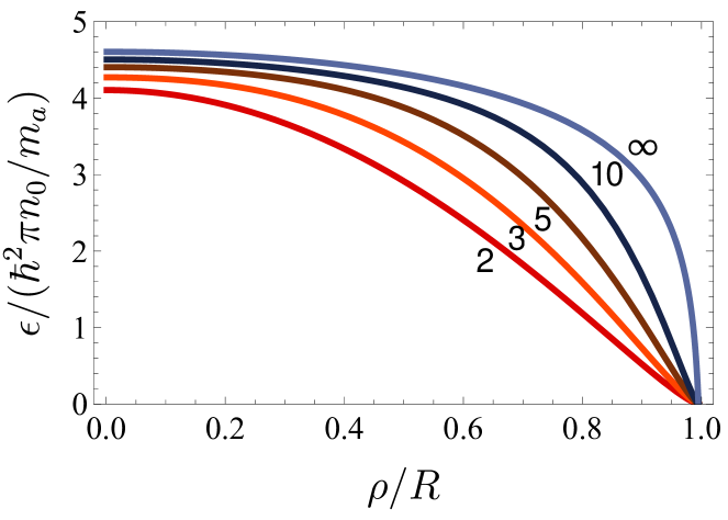
Figure 1: Dimensionless function $\epsilon(\rho)$ defined in Eq. (15) for different values of $k$ (given by the numbers next to the lines).

For a flat potential ($k\to\infty$), we have $\epsilon_{\infty}=\ln(1-\rho^{2})$, reproducing the usual result Richaud et al. (2020, 2021)

$$\Omega_{\infty}=\frac{\hbar\,q}{m_{a}R^{2}}\,\frac{1}{1-\rho^{2}},$$ (18)

now rewritten in conventional units. For the harmonic potential with $k=2$, we have

$$\epsilon_{2}=(1-\rho^{2})\left[\frac{(1+\rho^{2})\ln(1-\rho^{2})}{2\rho^{2}}-\ln\delta(\rho)\right],$$ (19)

where the vortex-core cutoff $\delta(\rho)$ depends on the condensate density and is scaled with $R$.

Figure 2 shows the precession rate of a vortex in a single-component BEC for selected integer values of $k$ as a function of the vortex position $\rho$. The solid curves show Eq. (17) for the massive point vortex model studied here. The dots show the results from the time-dependent Gross-Pitaevskii equation (solved using variants of algorithms we employed in Ref. Richaud et al. (2021)). The close overlap between lines and dots confirms the accuracy of the time-dependent variational Lagrangian formalism.

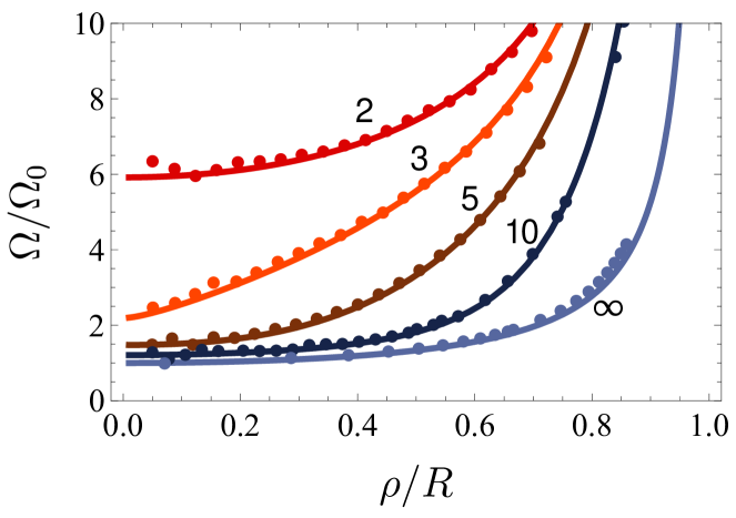
Figure 2: Dimensionless precession frequency $\Omega/\Omega_{0}$ [where $\Omega_{0}=\hbar/(m_{a}R^{2})$] for a vortex located at distance $\rho$ from the center of a single-component BEC in a power-law $r^{k}$ trap. Solid lines are the analytic predictions of Eq. (17), while dots show results from the full time-dependent GP equation. The numbers next to the lines denote the corresponding value of $k$.

For comparison with the study of the dynamics of a massive point vortex, which will be discussed in Sec. III, it is valuable to rewrite Eq. (16) in vector form

$$L_{a}=q\frac{\tau(\rho)}{\rho}\,\dot{\bm{\rho}}\times\hat{\bm{\rho}}\cdot\hat{\bm{z}}-\epsilon(\rho).$$ (20)

The corresponding canonical momentum

$$\bm{p}_{a}=\frac{\partial L_{a}}{\partial\dot{\bm{\rho}}}=q\frac{\tau(\rho)}{\rho}\hat{\bm{\rho}}\times\hat{\bm{z}}=-q\frac{\tau(\rho)}{\rho}\hat{\bm{\phi}}$$ (21)

is in the azimuthal direction, as expected for uniform circular motion. Note that the angular momentum is $\bm{l}=\bm{\rho}\times\bm{p}_{a}=-q\tau(\rho)\hat{\bm{z}}$, as found earlier.

The dynamics for this massless vortex follows from $\dot{\bm{p}}_{a}=\partial L_{a}/\partial\bm{\rho}$, which gives

$$\dot{\bm{p}}_{a}=q\left(\frac{\tau(\rho)}{\rho^{2}}-\frac{\tau^{\prime}(\rho)}{\rho}\right)\left(\dot{\bm{\rho}}\cdot\hat{\bm{\phi}}\right)\,\hat{\bm{\rho}}-\epsilon^{\prime}(\rho)\hat{\bm{\rho}}.$$ (22)

For uniform circular motion at fixed $\rho$, we note that $d\hat{\bm{\phi}}/dt=-\dot{\phi}\,\hat{\bm{\rho}}$ and a combination with Eq. (21) gives

$$\dot{\bm{p}}_{a}=q\frac{\tau(\rho)}{\rho}\dot{\phi}\,\hat{\bm{\rho}}=q\frac{\tau(\rho)}{\rho^{2}}\left(\dot{\bm{\rho}}\cdot\hat{\bm{\phi}}\right)\hat{\bm{\rho}},$$ (23)

so that some terms cancel. As a result, we find

$$0=\left[-2q(1-\rho^{k})\left(\dot{\bm{\rho}}\times\hat{\bm{z}}\cdot\hat{\bm{\rho}}\right)-\epsilon^{\prime}(\rho)\right]\hat{\bm{\rho}}.$$ (24)

The last term is the “force” arising from the negative gradient of the energy $\epsilon(\rho)$. In this picture, the vortex moves to ensure that the total force vanishes, which is precisely the “Magnus” effect. The resulting precession frequency reproduces the result given in Eq. (17), which follows more directly from the Lagrangian dynamics.

III Massive point vortex model

In the presence of a second component-$b$, the binary condensate obeys two coupled GP equations:

$$i\hbar\frac{\partial\Psi_{i}}{\partial t}=\!\!\left(\!-\frac{\hbar^{2}\nabla^{2}}{2m_{i}}+V_{\rm tr}+\sum_{j=a,b}g_{ij}|\Psi_{j}|^{2}\!\right)\Psi_{i},\;i=a,b$$ (25)

where $g_{ij}=\sqrt{2\pi}\hbar^{2}a_{ij}/(m_{ij}d_{z})$ represents the effective interactions in the quasi-2D system, with $a_{ij}$ being the intra- and inter-component $s$-wave scattering lengths and $m_{ij}=(m_{i}^{-1}+m_{j}^{-1})^{-1}$ are the reduced atomic masses Hadzibabic and Dalibard (2011). In the immiscible regime $g_{ab}>\sqrt{g_{aa}g_{bb}}$, the coupled equations (25) admit solutions where vortices are present in component-$a$ and wavepackets of $b$-particles are trapped within the vortices’ cores. The dynamics of these composite objects (which we term “massive vortices”) can be conveniently described with an effective particle-like model Richaud et al. (2020, 2021) which allows one to bypass the numerical solution of the GP equations (25).

In our model for a massive point vortex, the total Lagrangian is the previous $L_{a}$ for the $a$ component augmented by the Lagrangian $L_{b}$ for the $b$ component. We remark that the presence of $N_{b}\ll N_{a}$ atoms within the vortex core does not significantly change its shape and width (see Ref. Richaud et al. (2020) for the case of a ${}^{23}{\mathrm{Na}}-{}^{39}\mathrm{K}$ mixture and Ref. Richaud et al. (2022) for the case of a ${}^{87}{\mathrm{Rb}}-{}^{41}\mathrm{K}$ mixture), so that Eq. (7) remains valid. As discussed in detail in Ref. Richaud et al. (2021), $L_{b}$ is proportional to $N_{b}$, with a kinetic term $\frac{1}{2}N_{b}m_{b}\dot{\bm{\rho}}^{2}$. The new feature here is the trap potential, so that $L_{b}=\frac{1}{2}N_{b}m_{b}\dot{\bm{\rho}}^{2}-N_{b}V_{\rm tr}(\rho)$. With our dimensionless variables, $L_{b}$ is

$$L_{b}=\textstyle{\frac{1}{2}}{\mathfrak{m}}\dot{\bm{\rho}}^{2}-\nu\rho^{k}=\textstyle{\frac{1}{2}}{\mathfrak{m}}(\dot{\rho}^{2}+\rho^{2}\dot{\phi}^{2})-\nu\rho^{k},$$ (26)

where ${\mathfrak{m}}=M_{b}/M_{a}=N_{b}m_{b}/(N_{a}m_{a})$ is the ratio of the total $b$ mass to the total $a$ mass, and $\nu=N_{b}g_{aa}m_{a}/(\hbar^{2}\pi)$. Note that $\nu$ is proportional to the product $N_{b}g_{aa}$ and independent of $n_{0}$.

Our massive point-vortex model is expected to describe correctly the dynamics of a single massive vortex (and also a few massive vortices) as long as the component-$b$ atoms remain localized in the component-$a$ vortex cores, and as long as the $b$-atoms do not significantly alter the typical core size of component-$a$ bare vortices so that their cores remain much smaller than the TF radius $R$. The assumed immiscibility of the two components ensures the first condition, and the second one holds provided that $g_{aa}N_{a}$ is substantially larger than both $g_{ab}N_{b}$ and $g_{bb}N_{b}$. Note that the ratio $g_{bb}/g_{aa}$ does not enter the effective point-like model explicitly.

III.1 Total Lagrangian for massive point vortex

In this way the Lagrangian $L$ for a single massive point vortex becomes

$$L=\textstyle{\frac{1}{2}}{\mathfrak{m}}(\dot{\rho}^{2}+\rho^{2}\dot{\phi}^{2})-q\tau(\rho)\dot{\phi}-\epsilon(\rho)-\nu\rho^{k},$$ (27)

here written in coordinate form. It is helpful also to rewrite $L$ in vector form as

$$L={\textstyle{\frac{1}{2}}}{\mathfrak{m}}\dot{\bm{\rho}}^{2}+q\bm{A}(\rho)\cdot\dot{\bm{\rho}}-\epsilon(\rho)-\nu\rho^{k},$$ (28)

where

$$\bm{A}(\bm{\rho})=-\frac{\tau(\rho)}{\rho}\hat{\bm{\phi}}.$$ (29)

The Lagrangian has an unusual structure with a term linear in the velocity $\dot{\bm{\rho}}$ in addition to the usual quadratic term proportional to the inertial mass.

Such a Lagrangian is reminiscent of the Lagrangian $L_{\rm em}$ for a charged particle at $\bm{\rho}$ in an external electromagnetic field

$$L_{\rm em}={\textstyle{\frac{1}{2}}}{\mathfrak{m}}\dot{\bm{\rho}}^{2}+q\dot{\bm{\rho}}\cdot\bm{A}-q\,\Phi,$$ (30)

where $q$ is the charge, $\bm{A}$ is the vector potential and $\Phi$ is the scalar potential. The first two terms of Eqs. (28) and (30) are the same. The third term of Eq. (28) arises from the energy (12) of the vortex and its image. It is quadratic in the vortex charge and hence proportional to $q^{2}$, which here is simply $1$. The last term in (28) is the trap potential and hence independent of $q$.

Equation (28) gives the canonical momentum

$$\bm{p}=\frac{\partial L}{\partial\dot{\bm{\rho}}}={\mathfrak{m}}\dot{\bm{\rho}}+q\bm{A}.$$ (31)

The corresponding Hamiltonian

$$H=\frac{\left(\bm{p}-q\bm{A}\right)^{2}}{2{\mathfrak{m}}}+\epsilon+\nu\rho^{k}$$ (32)

is independent of $t$, so that $H$ is constant (here, it is the energy, expressed in Hamiltonian variables $\bm{p}$ and $\bm{\rho}$).

Equation (32) identifies $\bm{A}$ in (29) as a synthetic (or artificial) gauge field acting on the massive vortex. Note that $\tau$ appearing in $\bm{A}$ involves an integral over the TF density $n_{a}(\rho)$. Although we here study a power-law trap, other more general cylindrically symmetric TF densities could in principle be generated Zou et al. (2021), leading to different forms for $\tau(\rho)$ and hence for $\bm{A}$.

The corresponding synthetic magnetic field is

$$\bm{B}(\bm{\rho})=\bm{\nabla}\times\bm{A}(\bm{\rho})=-2\pi\hbar n_{a}(\rho)\hat{\bm{z}},$$ (33)

here expressed in conventional units. It is nonuniform except for a flat trap ($k\to\infty$), but the total flux obtained as $\int d^{2}\rho\,B_{\rm eff}(\bm{\rho})=-2\pi\hbar N_{a}$ is independent of $k$.

III.2 Dynamics of a massive point vortex

Equation (31) shows that the canonical momentum has an extra term proportional to the synthetic gauge field $\bm{A}$. An important consequence is the presence of synthetic angular momentum, even for a massless vortex in a flat potential with a circular boundary, as noted in Sec. II.A of Richaud et al. (2021). In the present case of a massive point vortex, we now show that its angular momentum has the usual term proportional to the mass and the angular velocity, but it also includes a second term arising from the synthetic gauge field. Similar contributions are common in electromagnetism Purcell (1985); Jackson (1998).

Since $L$ is independent of $\phi$, the angular momentum $l=\partial L/\partial\dot{\phi}$ of the massive vortex is conserved, with

$$l={\mathfrak{m}}\rho^{2}\dot{\phi}-q\tau(\rho).$$ (34)

Unlike the massless case, the angular momentum of a massive vortex can now have either sign. This unusual feature arises from the synthetic gauge field $\bm{A}=-[\tau(\rho)/\rho]\hat{\bm{\phi}}$. Here, the synthetic contribution is negative for a positive vortex, so that the total angular momentum can be negative for a vortex precessing uniformly in the positive direction. In addition, the angular momentum $l$ can vanish even for a precessing vortex, again owing to the synthetic contribution.

The associated radial motion follows directly as

$${\mathfrak{m}}\ddot{\rho}=\frac{\partial L}{\partial\rho}={\mathfrak{m}}\rho\dot{\phi^{2}}-q\tau^{\prime}(\rho)\dot{\phi}-\epsilon^{\prime}(\rho)-k\nu\rho^{k-1}.$$ (35)

Some manipulation gives the energy equation

$$\frac{1}{2}{\mathfrak{m}}\dot{\rho}^{2}+V_{\rm eff}(\rho)=\hbox{constant},$$ (36)

with the effective potential

$$V_{\rm eff}(\rho)=\frac{[l+q\tau(\rho)]^{2}}{2{\mathfrak{m}}\rho^{2}}+\epsilon(\rho)+\nu\rho^{k}.$$ (37)

Equation (36) expresses the conservation of energy in Lagrangian variables $\dot{\bm{\rho}}$ and $\bm{\rho}$, which are generally more useful than the Hamiltonian variables. In particular, the general radial dynamical equation becomes

$${\mathfrak{m}}\ddot{\rho}=-V_{\rm eff}^{\prime}(\rho),$$ (38)

balancing the Newtonian acceleration ${\mathfrak{m}}\ddot{\rho}$ and the force $-V^{\prime}_{\rm eff}(\rho)$.

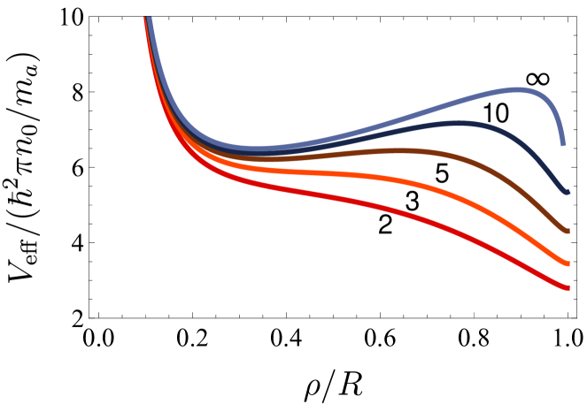
Figure 3: Plot of the effective potential (37) as a function of the radial distance $\rho$, here shown for several values of $k$ and fixed $l=\mathfrak{m}=0.1$ and $\nu=1$. The numbers next to the lines denote the corresponding value of $k$.

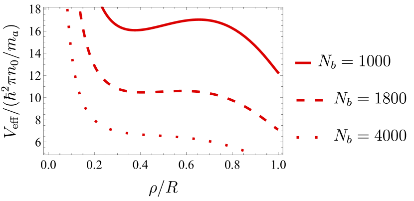
Figure 4: Plot of the effective potential (37) as a function of the radial distance $\rho$, here expressed for several values of $N_{b}$ and fixed $k=2$, $l=0.1$, $\mathfrak{m}=1.5\times 10^{-5}N_{b}$, $\nu=2.5\times 10^{-4}N_{b}$.

In many cases, $V_{\rm eff}(\rho)$ has a single local minimum at a position $\rho_{0}$ that depends on the parameters $l$, ${\mathfrak{m}}$, and $\nu$. Figure 3 shows that the presence of the minimum depends sensitively on $k$. For a given mass ratio $\mathfrak{m}$ the flat trap ($k\to\infty$) has a local minimum, but the latter disappears when $k$ decreases beyond a critical value. The minimum also disappears as the number $N_{b}$ of atoms in the core increases, as shown in Fig. 4.

For small $\mathfrak{m}\ll 1$, we can ignore the last two terms of (37) and focus on the first term. If $l$ is also small, the minimum occurs at small $\rho_{0}\approx\sqrt{l}$, confirming that there is always a local minimum, as expected from the behavior for a pure $a$ condensate.

If the effective potential has a local minimum at $\rho_{0}$, a massive point vortex at this radial distance from the origin precesses uniformly at a rate obtained by setting the right side of Eq. (35) to zero. The resulting precession frequency $\Omega$ now satisfies a quadratic equation

$${\mathfrak{m}}\rho_{0}\Omega^{2}-q\tau^{\prime}(\rho_{0})\Omega-\epsilon^{\prime}(\rho_{0})-k\nu\rho_{0}^{k-1}=0.$$ (39)

The first and last terms arise from the presence of the vortex mass, since both ${\mathfrak{m}}$ and $\nu$ are proportional to $N_{b}$. In contrast, the second and third terms are just those studied in the previous section, including both the Magnus effect and the variational energy $\epsilon(\rho)$. Thus Eq. (39) includes all the physics inherent in our combined Lagrangian $L=L_{a}+L_{b}$.

For small $N_{b}$, both ${\mathfrak{m}}$ and $\nu$ are small, and the first and last terms in (39) become negligible. In this limit, the single root of Eq. (39) reproduces Eq. (17) for a massless vortex.

As $N_{b}$ increases, however, Eq. (39) has two finite solutions; a massive point vortex at a given radial distance $\rho_{0}$ then has two distinct modes with different precession frequencies. With positive $q$, the larger root

$$\Omega_{+}=\frac{\tau^{\prime}(\rho_{0})+\sqrt{\tau^{\prime}(\rho_{0})^{2}+4{\mathfrak{m}}\rho_{0}\left[\epsilon^{\prime}(\rho_{0})+k\nu\rho_{0}^{k-1}\right]}}{2{\mathfrak{m}}\rho_{0}}$$ (40)

diverges for small mass ratio ${\mathfrak{m}}\ll 1$.

In contrast, the smaller root $\Omega_{-}$ is more physically significant because it remains finite for small $\mathfrak{m}$

$$\Omega_{-}=\frac{2\left[-\epsilon^{\prime}(\rho_{0})-k\nu\rho_{0}^{k-1}\right]}{\tau^{\prime}(\rho_{0})+\sqrt{\tau^{\prime}(\rho_{0})^{2}+4{\mathfrak{m}}\rho_{0}\left[\epsilon^{\prime}(\rho_{0})+k\nu\rho_{0}^{k-1}\right]}}.$$ (41)

The denominator of Eq. (41) is generally positive (as discussed below, it can be complex, which implies instability). In contrast, the numerator can have either sign, depending on the vortex position $\rho_{0}$ and the dimensionless parameter $\nu$, which depends linearly on $N_{b}$. The quantity $-\epsilon^{\prime}(\rho_{0})$ is positive (see Fig. 1), but $-k\nu\rho_{0}^{k-1}$ is negative. For small $N_{b}$ and $\nu$, the energy term with $-\epsilon^{\prime}$ dominates and the positive massive vortex precesses in the positive sense. For larger $\nu$, however, the derivative of the trap potential dominates, and a positive vortex now precesses in the negative direction.

Figure 5 illustrates this situation for several integer values of $k$. Ruban Ruban (2022) independently found similar behavior for $k=2$ with a hydrodynamic model based on two coupled GP equations. In our model of a massive point vortex, the effect is most pronounced for the harmonic trap ($k=2$), and is absent for the flat trap ($k\to\infty$), as found in Ref. Richaud et al. (2021).

It is notable that the JILA two-component experiment with two hyperfine states of ⁸⁷Rb (see Fig. 2 of Anderson et al. (2000)) and the associated theoretical analysis (see Fig. 4 of  McGee and Holland (2001)) both found examples with negative precession frequencies, although it is not clear that they arose from the same mechanism. In the experiment, the three interaction constants here are nearly equal, so that these results are definitely not in the regime of a well-localized core state. It would be desirable to have additional experiments with two different atoms, such as our proposed ²³Na and ³⁹K mixture.

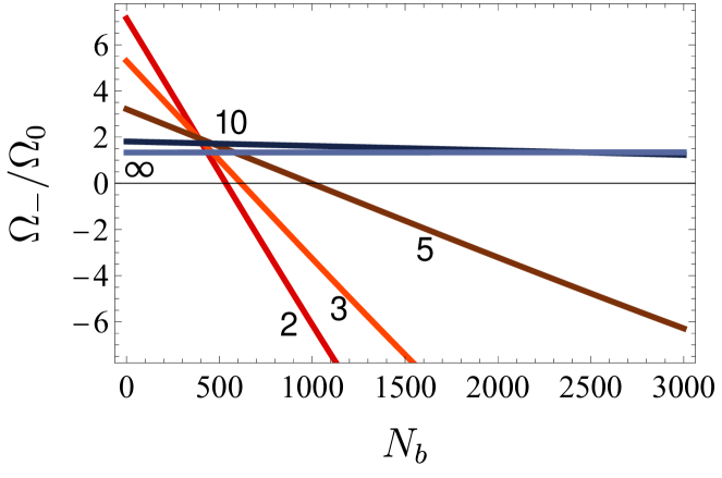
Figure 5: The precession frequency $\Omega_{-}$ [see Eq. (41)] is positive for small core masses, but it can vanish and become negative as the number $N_{b}$ of component-$b$ core atoms increases. Here $\mathfrak{m}=3\times 10^{-6}N_{b}$, $\nu=10^{-2}N_{b}$ and $\Omega_{0}=\hbar/(m_{a}R^{2})$, which are typical values for a vortex in a BEC composed of $6\times 10^{5}$ ²³Na atoms (pancake-shaped, with $R\sim 50~{}\mu$m and $d_{z}\sim 1~{}\mu$m), with the vortex mass provided by $N_{b}$ ³⁹K atoms (see Ref. Richaud et al. (2019) for additional details about the tunability of intra- and interspecies coupling strengths in this specific Bose-Bose mixture). The numbers next to the lines denote the corresponding value of $k$.

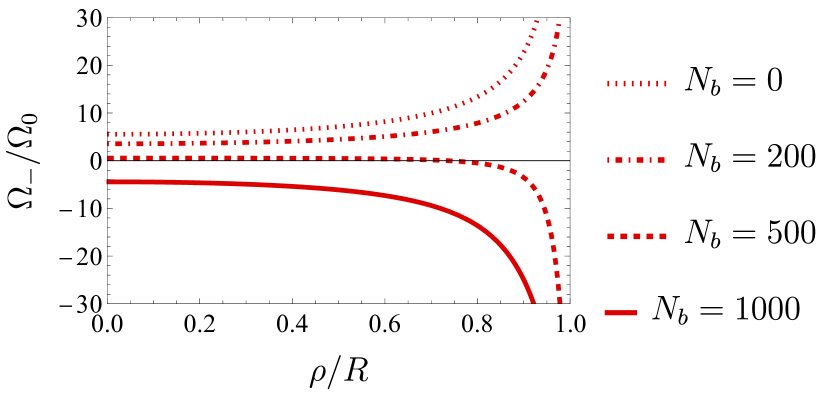
Figure 6: The precession frequency $\Omega_{-}$ [see Eq. (41)] for $k=2$. It is positive for small core masses, but it can vanish and become negative as the number $N_{b}$ of component-$b$ core atoms increases. We employ the same microscopic model parameters used in Fig. 5, which yield $\mathfrak{m}=3\times 10^{-6}N_{b}$ and $\nu=10^{-2}N_{b}$. The normalization frequency $\Omega_{0}$ reads $\Omega_{0}=\hbar/(m_{a}R^{2})$.

The connection between the two roots $\Omega_{\pm}$ and the single local minimum $\rho_{0}$ may be understood by starting from parameters $\mathfrak{m},l$ and $\nu$ that give a clear minimum such as the upper curve in Fig. 4. These values then yield $\Omega_{\pm}$ from Eqs. (40) and (41). Use these frequencies to find the corresponding angular momenta $l_{\pm}$ from (34). One of the solutions is the same as the input in finding the minimum of $V_{\rm eff}(\rho_{0})$, but the other solution gives a second distinct $V_{\rm eff}(\rho_{0})$. Although both effective potential curves have minima at the same $\rho_{0}$, they have different $l_{\pm}$ and therefore different detailed shapes.

Equation (39) has real coefficients, so that its roots are either real or complex conjugates, depending on the sign of the discriminant

$${\cal D}=\tau^{\prime}(\rho_{0})^{2}+4{\mathfrak{m}}\rho_{0}\left[\epsilon^{\prime}(\rho_{0})+k\nu\rho_{0}^{k-1}\right].$$ (42)

The quantity $\epsilon^{\prime}(\rho_{0})$ is negative and $k\nu\rho_{0}^{k-1}$ is positive, so that their sum can have either sign. The two roots $\Omega_{\pm}$ are usually real, but, depending on the assumed values for the parameter $g_{aa}$ and the mass ratio $\mathfrak{m}$, they can become complex-conjugate pairs, indicating that the vortex will not precess but instead drift to the outer boundary. In Ref. Richaud et al. (2021) we found that $\cal D$ in a flat trap was negative for $2{\mathfrak{m}}>1-\rho_{0}^{2}$ , and we here generalize the discussion for general $k$.

III.3 Stability of uniform precession for massive vortex

If $V_{\rm eff}(\rho)$ has a local minimum at $\rho_{0}$, then the stability of the uniform precession follows by expanding around the minimum, with $\rho=\rho_{0}+\delta$. Since $V_{\rm eff}^{\prime}(\rho_{0})$ vanishes at a local minimum, the leading terms from Eq. (38) become

$${\mathfrak{m}}\ddot{\delta}+V_{\rm eff}^{\prime\prime}(\rho_{0})\,\delta=0.$$ (43)

This equation describes a simple harmonic oscillator with squared frequency

$$\omega^{2}=\frac{V_{\rm eff}^{\prime\prime}(\rho_{0})}{\mathfrak{m}},$$ (44)

where the local curvature $V_{\rm eff}^{\prime\prime}(\rho_{0})$ serves as an effective spring constant.

An equivalent procedure is to expand the pair of Euler-Lagrange equations for $\rho$ and $\phi$ around the stable precessing motion, with $\rho=\rho_{0}+\delta\rho$ and $\phi=\Omega t+\delta\phi$. For example, the linearized form of Eq. (34) gives

$$\left[2{\mathfrak{m}}\rho_{0}\Omega-q\tau^{\prime}(\rho_{0})\right]\delta\rho+{\mathfrak{m}}\rho_{0}^{2}\delta\dot{\phi}=0.$$ (45)

With harmonic time dependence $\propto e^{-i\omega t}$, it is clear that the two perturbations $\delta\rho$ and $\delta\phi$ are out of phase because of the relative factor $i$. A combination with the linearized form of the other dynamical equation (35) readily gives the same oscillation frequency as in Eq. (44). Figure 7 shows typical perturbed trajectories for both signs of the precession frequency $\Omega_{-}$.

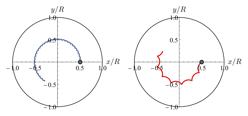
Figure 7: Perturbed uniform circular orbits of a positive vortex for $k=\infty$ (left panel) and $k=2$ (right panel). Black dots correspond to the initial positions. The precession frequency, given by Eq. (41), is positive in the first case and negative in the second. The frequency of small-amplitude radial oscillations is given by Eq. (44). Here we used $\mathfrak{m}=0.03$, $\nu=10$ and $\delta_{0}=0.005$.

Figures 3 and 4 indicate that the effective potential resembles a cubic curve with a single local minimum and a single local maximum. The local minimum (maximum) is stable (unstable) with positive (negative) curvature. As the parameters vary, the two stationary points can merge and form a single inflection point, which signals the onset of instability. Beyond this point, the radial position obeys the simple Newtonian dynamical equation ${\mathfrak{m}}\ddot{\rho}=-V_{\rm eff}^{\prime}(\rho)$. In this case, the vortex will move to the outer boundary of the condensate.

IV Conclusions and Outlook

In this paper, we constructed a two-dimensional Lagrangian $L=L_{a}+L_{b}$ for a massive point vortex in a power-law trap potential $\propto r^{k}$. Our model assumes a singly quantized vortex in condensate $a$ surrounding a localized condensate $b$ that provides an inertial mass. The power-law potential allows an interpolation between the harmonic trap ($k=2$) and the flat trap with a rigid circular boundary ($k\to\infty$). For an empty-core vortex in the pure $a$ component, the model Lagrangian $L_{a}$ leads to first-order dynamical equations with uniform circular precession for all values of $k$.

To include the inertial effect of the core, we added the Lagrangian $L_{b}$ derived in Richaud et al. (2021), now generalized to the power-law trap. The total Lagrangian for the vortex coordinate $\bm{\rho}=(\rho,\phi)$ is axisymmetric and therefore conserves the total angular momentum $l$. Unusually, $l$ includes not only the usual Newtonian inertial part $\propto\bm{\rho}\times\dot{\bm{\rho}}=\rho^{2}\dot{\phi}$ but also a contribution from a synthetic gauge field associated with the vortex. It is notable that synthetic gauge fields have served to create massless vortices Lin et al. (2009), whereas here we identify a (density-dependent) synthetic gauge field that acts on a massive point vortex. DMDs (digital micromirror devices) Zou et al. (2021) allow experiments with almost arbitrary condensate shapes, including time periodic structures. The corresponding time-periodic synthetic gauge fields could combine superfluid vortex dynamics with Floquet physics Eckardt (2017) and Thouless pumping Ozawa et al. (2019).

Manipulation of the coupled dynamical equations for $\rho$ and $\phi$ leads to an effective potential $V_{\rm eff}(\rho)$ and an explicit radial dynamical equation ${\mathfrak{m}}\ddot{\rho}=-V_{\rm eff}^{\prime}(\rho)$, where ${\mathfrak{m}}=M_{b}/M_{a}$ is the mass ratio. For small enough values of $\mathfrak{m}$ and $l$, $V_{\rm eff}(\rho)$ has a single local minimum, where stable uniform circular motion can occur. For larger $\mathfrak{m}$, however, the local minimum disappears and the vortex spirals outward to the trap edge.

We studied the precession of a massive vortex for various values of the parameters in the Lagrangian such as the mass ratio ${\mathfrak{m}}=M_{b}/M_{a}$, the coupling strength $\nu=N_{b}g_{aa}m_{a}/(\hbar^{2}\pi)$ between the vortex and the trap, and the exponent $k$ of the trap potential. For a flat potential ($k\rightarrow\infty$), a positive massive vortex always precesses in the positive sense, independent of the number $N_{b}$ of $b$-component atoms which provide its mass. For finite $k$, however, the precession can reverse direction with increasing $N_{b}$. The effect is stronger for smaller $k$ and therefore should be most easily observable in the usual case of harmonic trapping ($k=2$).

As noted toward the end of Sec. III.B, the early JILA experiment Anderson et al. (2000) detected several two-component vortices that precessed in the reverse direction. These experiments relied on two hyperfine states of ⁸⁷Rb, where the interaction constants $g_{jk}$ are nearly identical. In contrast, our model assumes different atomic species ²³Na and ³⁹K with the conditions $g_{aa}g_{bb}\ll g_{ab}^{2}$ to be deep in the phase-separated regime and $g_{aa}N_{a}\gg g_{ab}N_{b},\,g_{bb}N_{b}$ to ensure that the size of a vortex in component $a$ is barely modified by the $b$ impurities in its core. It would be very interesting to study vortices in two-component systems with small core radii and perhaps detect the reversal of precession as the minority component increases.

References

- Feynman (1955) R. P. Feynman, in Progress in Low Temperature Physics, Vol. 1 (Elsevier, North-Holland, Amsterdam, 1955) pp. 17–53.
- Pethick and Smith (2008) C. J. Pethick and H. Smith, Bose-Einstein Condensation in Dilute Gases (Cambridge University Press, Cambridge, 2008) 2nd ed.
- Pitaevskii and Stringari (2016) L. Pitaevskii and S. Stringari, Bose-Einstein Condensation and Superfluidity (Oxford University Press, Oxford, 2016) 2nd ed.
- Matthews et al. (1999) M. R. Matthews, B. P. Anderson, P. C. Haljan, D. S. Hall, C. E. Wieman, and E. A. Cornell, Vortices in a Bose-Einstein Condensate, Phys. Rev. Lett. 83, 2498 (1999).
- Anderson et al. (2000) B. P. Anderson, P. C. Haljan, C. E. Wieman, and E. A. Cornell, Vortex Precession in Bose-Einstein Condensates: Observations with Filled and Empty Cores, Phys. Rev. Lett. 85, 2857 (2000).
- Madison et al. (2000) K. W. Madison, F. Chevy, W. Wohlleben, and J. Dalibard, Vortex Formation in a Stirred Bose-Einstein Condensate, Phys. Rev. Lett. 84, 806 (2000).
- Raman et al. (2001) C. Raman, J. R. Abo-Shaeer, J. M. Vogels, K. Xu, and W. Ketterle, Vortex Nucleation in a Stirred Bose-Einstein Condensate, Phys. Rev. Lett. 87, 210402 (2001).
- Leanhardt et al. (2002) A. E. Leanhardt, A. Görlitz, A. P. Chikkatur, D. Kielpinski, Y. Shin, D. E. Pritchard, and W. Ketterle, Imprinting Vortices in a Bose-Einstein Condensate using Topological Phases, Phys. Rev. Lett. 89, 190403 (2002).
- Scherer et al. (2007) D. R. Scherer, C. N. Weiler, T. W. Neely, and B. P. Anderson, Vortex Formation by Merging of Multiple Trapped Bose-Einstein Condensates, Phys. Rev. Lett. 98, 110402 (2007).
- Kwon et al. (2016) W. J. Kwon, J. H. Kim, S. W. Seo, and Y. Shin, Observation of von Kármán Vortex Street in an Atomic Superfluid Gas, Phys. Rev. Lett. 117, 245301 (2016).
- Freilich et al. (2010) D. V. Freilich, D. M. Bianchi, A. M. Kaufman, T. K. Langin, and D. S. Hall, Real-Time Dynamics of Single Vortex Lines and Vortex Dipoles in a Bose-Einstein Condensate, Science 329, 1182 (2010).
- Serafini et al. (2017) S. Serafini, L. Galantucci, E. Iseni, T. Bienaimé, R. N. Bisset, C. F. Barenghi, F. Dalfovo, G. Lamporesi, and G. Ferrari, Vortex Reconnections and Rebounds in Trapped Atomic Bose-Einstein Condensates, Phys. Rev. X 7, 021031 (2017).
- Kwon et al. (2021) W. Kwon, G. Del Pace, K. Xhani, L. Galantucci, A. Muzi Falconi, M. Inguscio, F. Scazza, and G. Roati, Sound emission and annihilations in a programmable quantum vortex collider, Nature 600, 64 (2021).
- Richaud et al. (2022) A. Richaud, G. Lamporesi, M. Capone, and A. Recati, Mass-driven vortex collisions in flat superfluids, arXiv preprint arXiv:2209.00493 (2022).
- Lundh and Ao (2000) E. Lundh and P. Ao, Hydrodynamic approach to vortex lifetimes in trapped Bose condensates, Phys. Rev. A 61, 063612 (2000).
- McGee and Holland (2001) S. A. McGee and M. J. Holland, Rotational dynamics of vortices in confined Bose-Einstein condensates, Phys. Rev. A 63, 043608 (2001).
- Richaud et al. (2020) A. Richaud, V. Penna, R. Mayol, and M. Guilleumas, Vortices with massive cores in a binary mixture of Bose-Einstein condensates, Phys. Rev. A 101, 013630 (2020).
- Griffin et al. (2020) A. Griffin, V. Shukla, M.-E. Brachet, and S. Nazarenko, Magnus-force model for active particles trapped on superfluid vortices, Phys. Rev. A 101, 053601 (2020).
- Richaud et al. (2021) A. Richaud, V. Penna, and A. L. Fetter, Dynamics of massive point vortices in a binary mixture of Bose-Einstein condensates, Phys. Rev. A 103, 023311 (2021).
- Ruban (2022) V. P. Ruban, Direct and Reverse Precession of a Massive Vortex in a Binary Bose-Einstein Condensate, JETP Lett. 115, 415 (2022).
- Doran et al. (2022) R. Doran, A. W. Baggaley, and N. G. Parker, Vortex Solutions in a Binary Immiscible Bose-Einstein Condensate, arXiv:2207.12913 (2022).
- Navon et al. (2021) N. Navon, R. P. Smith, and Z. Hadzibabic, Quantum gases in optical boxes, Nat. Phys. 17, 1334 (2021).
- Zou et al. (2021) Y.-Q. Zou, É. Le Cerf, B. Bakkali-Hassani, C. Maury, G. Chauveau, P. C. M. Castilho, R. Saint-Jalm, S. Nascimbene, J. Dalibard, and J. Beugnon, Optical control of the density and spin spatial profiles of a planar Bose gas, J. Phys. B: At. Mol. Opt. Phys. 54, 08LT01 (2021).
- Groszek et al. (2018) A. J. Groszek, D. M. Paganin, K. Helmerson, and T. P. Simula, Motion of vortices in inhomogeneous Bose-Einstein condensates, Phys. Rev. A 97, 023617 (2018).
- Jackson et al. (1999) B. Jackson, J. F. McCann, and C. S. Adams, Vortex line and ring dynamics in trapped Bose-Einstein condensates, Phys. Rev. A 61, 013604 (1999).
- Svidzinsky and Fetter (2000a) A. A. Svidzinsky and A. L. Fetter, Stability of a Vortex in a Trapped Bose-Einstein Condensate, Phys. Rev. Lett. 84, 5919 (2000a).
- Svidzinsky and Fetter (2000b) A. A. Svidzinsky and A. L. Fetter, Dynamics of a vortex in a trapped Bose-Einstein condensate, Phys. Rev. A 62, 063617 (2000b).
- Kim and Fetter (2004) J.-K. Kim and A. L. Fetter, Dynamics of a single ring of vortices in two-dimensional trapped Bose-Einstein condensates, Phys. Rev. A 70, 043624 (2004).
- Anglin (2002) J. R. Anglin, Vortices near surfaces of Bose-Einstein condensates, Phys. Rev. A 65, 063611 (2002).
- Sheehy and Radzihovsky (2004) D. E. Sheehy and L. Radzihovsky, Vortices in spatially inhomogeneous superfluids, Phys. Rev. A 70, 063620 (2004).
- Jezek and Cataldo (2008) D. M. Jezek and H. M. Cataldo, Vortex velocity field in inhomogeneous media: A numerical study in Bose-Einstein condensates, Phys. Rev. A 77, 043602 (2008).
- dos Santos (2016) F. E. A. dos Santos, Hydrodynamics of vortices in Bose-Einstein condensates: A defect-gauge field approach, Phys. Rev. A 94, 063633 (2016).
- Esposito et al. (2017) A. Esposito, R. Krichevsky, and A. Nicolis, Vortex precession in trapped superfluids from effective field theory, Phys. Rev. A 96, 033615 (2017).
- Biasi et al. (2017) A. Biasi, P. Bizoń, B. Craps, and O. Evnin, Exact lowest-Landau-level solutions for vortex precession in Bose-Einstein condensates, Phys. Rev. A 96, 053615 (2017).
- Lamb (1945) H. Lamb, Hydrodynamics (Dover, New York, 1945) Chap. 7, 6th ed.
- Hadzibabic and Dalibard (2011) Z. Hadzibabic and J. Dalibard, Two-dimensional Bose fluids: An atomic physics perspective, La Rivista del Nuovo Cimento 34, 389 (2011).
- Pérez-García et al. (1996) V. M. Pérez-García, H. Michinel, J. I. Cirac, M. Lewenstein, and P. Zoller, Low Energy Excitations of a Bose-Einstein Condensate: A Time-Dependent Variational Analysis, Phys. Rev. Lett. 77, 5320 (1996).
- Purcell (1985) E. M. Purcell, Electricity and Magnetism, 2nd Edition (McGraw-Hill, New York, 1985) p. 450.
- Jackson (1998) J. D. Jackson, Classical Electrodynamics, 3rd Edition (Wiley, Hoboken, 1998) p. 350.
- Richaud et al. (2019) A. Richaud, A. Zenesini, and V. Penna, The mixing-demixing phase diagram of ultracold heteronuclear mixtures in a ring trimer, Sci. Rep. 9, 6908 (2019).
- Lin et al. (2009) Y.-J. Lin, R. L. Compton, K. Jiménez-García, J. V. Porto, and I. B. Spielman, Synthetic magnetic fields for ultracold neutral atoms, Nature 462, 628 (2009).
- Eckardt (2017) A. Eckardt, Colloquium: Atomic quantum gases in periodically driven optical lattices, Rev. Mod. Phys. 89, 011004 (2017).
- Ozawa et al. (2019) T. Ozawa, H. M. Price, A. Amo, N. Goldman, M. Hafezi, L. Lu, M. C. Rechtsman, D. Schuster, J. Simon, O. Zilberberg, and I. Carusotto, Topological photonics, Rev. Mod. Phys. 91, 015006 (2019).