Almost-Orthogonal Layers for Efficient General-Purpose Lipschitz Networks

Abstract

It is a highly desirable property for deep networks to be robust against small input changes. One popular way to achieve this property is by designing networks with a small Lipschitz constant. In this work, we propose a new technique for constructing such Lipschitz networks that has a number of desirable properties: it can be applied to any linear network layer (fully-connected or convolutional), it provides formal guarantees on the Lipschitz constant, it is easy to implement and efficient to run, and it can be combined with any training objective and optimization method. In fact, our technique is the first one in the literature that achieves all of these properties simultaneously.

Our main contribution is a rescaling-based weight matrix parametrization that guarantees each network layer to have a Lipschitz constant of at most $1$ and results in the learned weight matrices to be close to orthogonal. Hence we call such layers almost-orthogonal Lipschitz (AOL).

Experiments and ablation studies in the context of image classification with certified robust accuracy confirm that AOL layers achieve results that are on par with most existing methods. Yet, they are simpler to implement and more broadly applicable, because they do not require computationally expensive matrix orthogonalization or inversion steps as part of the network architecture.

We provide code at https://github.com/berndprach/AOL.

Keywords Lipschitz networks, orthogonality, robustness

1 Introduction

Deep networks are often the undisputed state of the art when it comes to solving computer vision tasks with high accuracy. However, the resulting systems tend to be not very robust, e.g., against small changes in the input data. This makes them untrustworthy for safety-critical high-stakes tasks, such as autonomous driving or medical diagnosis.

A typical example of this phenomenon are adversarial examples [1]: imperceptibly small changes to an image can drastically change the outputs of a deep learning classifier when chosen in an adversarial way. Since their discovery, numerous methods were developed to make networks more robust against adversarial examples. However, in response a comparable number of new attack forms were found, leading to an ongoing cat-and-mouse game. For surveys on the state of research, see, e.g., [2, 3, 4].

A more principled alternative is to create deep networks that are robust by design, for example, by restricting the class of functions they can represent. Specifically, if one can ensure that a network has a small Lipschitz constant, then one knows that small changes to the input data will not result in large changes to the output, even if the changes are chosen adversarially.

A number of methods for designing such Lipschitz networks have been proposed in the literature, which we discuss in Section 3. However, all of them have individual limitations. In this work, we introduce the AOL (for almost-orthogonal Lipschitz) method. It is the first method for constructing Lipschitz networks that simultaneously meets all of the following desirable criteria:

Generality. AOL is applicable to a wide range of network architectures, in particular most kinds of fully-connected and convolutional layers. In contrast, many recent methods work only for a restricted set of layer types, such as only fully-connected layers or only convolutional layers with non-overlapping receptive fields.

Formal guarantees. AOL provably guarantees a Lipschitz constant $1$. This is in contrast to methods that only encourage small Lipschitz constants, e.g., by regularization.

Efficiency. AOL causes only a small computational overhead at training time and none at all at prediction time. This is in contrast to methods that embed expensive iterative operations such as matrix orthogonalization or inversion steps into the network layers.

Modularity. AOL can be treated as a black-box module and combined with arbitrary training objective functions and optimizers. This is in contrast to methods that achieve the Lipschitz property only when combined with, e.g., specific loss-rescaling or projection steps during training.

AOL’s name stems from the fact that the weight matrices it learns are approximately orthogonal. In contrast to prior work, this property is not enforced explicitly, which would incur a computational cost. Instead, almost-orthogonal weight matrices emerge organically during network training. The reason is that AOL’s rescaling step relies on an upper bound to the Lipschitz constant that is tight for parameter matrices with orthogonal columns. During training, matrices without that property are put at the disadvantage of resulting in outputs of smaller dynamic range. As a consequence, orthogonal matrices are able to achieve smaller values of the loss and are therefore preferred by the optimizer.

2 Notation and Background

A function $f:\mathbb{R}^{n}\to\mathbb{R}^{m}$ is called $L$-Lipschitz continuous with respect to norms $\|.\|_{\mathbb{R}^{n}}$ and $\|.\|_{\mathbb{R}^{m}}$, if it fulfills

$$\|f(x)-f(y)\|_{\mathbb{R}^{m}}\leq L\|x-y\|_{\mathbb{R}^{n}},$$ (1)

for all $x$ and $y$, where $L$ is called the Lipschitz constant. In this work we only consider Lipschitz-continuity with respect to the Euclidean norm, $\|.\|_{2}$, and mainly for $L=1$. For conciseness of notation, we refer to such 1-Lipschitz continuous functions simply as Lipschitz functions.

For any linear (actually affine) function $f$, the Lipschitz property can be verified by checking if the function’s Jacobian matrix, $J_{f}$, has spectral norm $\|J_{f}\|_{\text{spec}}$ less or equal to $1$, where

$$[J_{f}]_{ij}=\frac{\partial f_{i}}{\partial x_{j}}\qquad\text{and}\qquad\|M\|_{\text{spec}}=\max_{\|v\|_{2}=1}\|Mv\|_{2}.$$ (2)

The spectral norm of a matrix $M$ can in fact be computed numerically as it is identical to the largest singular value of the matrix. This, however, typically requires iterative algorithms that are computationally expensive in high-dimensional settings. An exception is if $M$ is an orthogonal matrix, i.e. $M^{\top}M=I$, for $I$ the identity matrix. In that case we know that all its singular values are $1$ and $\|Mv\|_{2}=\|v\|_{2}$ for all $v$, so the corresponding linear transformation is Lipschitz.

Throughout this work we consider a deep neural network as a concatenation of linear layers (fully-connected or convolutional) alternating with non-linear activation functions. We then study the problem how to ensure that the resulting network function is Lipschitz.

It is known that computing the exact Lipschitz constant of a neural network is an NP-hard problem [5]. However, upper bounds can be computed more efficiently, e.g., by multiplying the individual Lipschitz constants of all layers.

3 Related work

The first attempts to train deep networks with small Lipschitz constant used ad-hoc techniques, such as weight clipping [6] or regularizing either the network gradients [7] or the individual layers’ spectral norms [8]. However, these techniques do not formally guarantee bounds on the Lipschitz constant of the trained network. Formal guarantees are provided by constructions that ensure that each individual network layer is Lipschitz. Combined with Lipschitz activation functions, such as ReLU, MaxMin or $\tanh$, this ensures that the overall network function is Lipschitz.

In the following, we discuss a number of prior methods for obtaining Lipschitz networks. A structured overview of their properties can be found in Table 1.

Table 1: Overview of the properties of different methods for learning Lipschitz networks. Columns indicate: E (efficiency): no internal iterative procedure required, scales well with the input size. F (formal guarantees): provides a guarantee about the Lipschitz constant of the trained network. G (generality): can be applied to fully-connected as well as convolutional layers. M (modularity): can be used with any training objective and optimization method.
$\sim$ symbols indicate that a property is partially fulfilled. Superscripts provide further explanations: ¹ requires a regularization loss. ² internal methods would have to be run to convergence. ³ iterative procedure that can be split between training steps. ⁴ requires matrix orthogonalization. ⁵ requires inversion of an input-sized matrix. ⁶ requires circular padding and full-image kernel size. ⁷ requires large kernel sizes to ensure orthogonality.

Method	E	F	G	M	Methodology
WGAN [6]	✓	✓	✓	✗	weight clipping
WGAN-GP [7]	✓	✗	✓	$\sim^{1}$	regularization
Parseval Networks [9]	✓	✗	✓	$\sim^{1}$	regularization
OCNN [10]	✓	✗	✓	$\sim^{1}$	regularization
SN [8]	✗	$\sim^{2}$	✓	✓	parameter rescaling
LCC [11]	✗	$\sim^{2}$	✓	✗	parameter rescaling
LMT [12]	$\sim^{3}$	✗	✓	✗	loss rescaling
GloRo [13]	$\sim^{3}$	$\sim^{2}$	✓	✗	loss rescaling
BCOP [14]	✗4	✓	✓	✓	explicit orthogonalization
GroupSort[15]	✗4	$\sim^{2}$	✗	✓	explicit orthogonalization
ONI [16]	✗	$\sim^{2}$	✓	✓	explicit orthogonalization
Cayley Convs [17]	$\sim^{5}$	✓	$\sim^{6}$	✓	explicit orthogonalization
SOP [18]	✗	$\sim^{2}$	$\sim^{7}$	✓	explicit orthogonalization
ECO [19]	✗4	✓	$\sim^{6}$	✓	explicit orthogonalization
AOL (proposed)	✓	✓	✓	✓	parameter rescaling

3.1 Bound-based methods

The Lipschitz property of a network layer could be achieved trivially: one simply computes the layer’s Lipschitz constant, or an upper bound, and divides the layer weights by that value. Applying such a step after training, however, does not lead to satisfactory results in practice, because the dynamic range of the network outputs is reduced by the product of the scale factors. This can be seen as a reduction of network capacity that prevents the network from fitting the training data well. Instead, it makes sense to incorporate the Lipschitz condition already at training time, such that the optimization can attempt to find weight matrices that lead to a network that is not only Lipschitz but also able to fit the data well.

The Lipschitz Constant Constraint (LCC) method [11] identifies all weight matrices with spectral norm above a threshold $\lambda$ after each weight update and rescales those matrices to have a spectral norm of exactly $\lambda$. Lipschitz Margin Training (LMT) [12] and Globally-Robust Neural Networks (GloRo) [13] approximate the overall Lipschitz constant from numeric estimates of the largest singular values of the layers’ weight matrices. They integrate this value as a scale factor into their respective loss functions.

In the context of deep learning, controlling only the Lipschitz constant of each layer separately has some drawbacks. In particular, the product of the individual Lipschitz constants might grossly overestimate the network’s actual Lipschitz constant. The reason is that the Lipschitz constant of a layer is determined by a single vector direction of maximal expansion. When concatenating multiple layers, their directions of maximal expansion will typically not be aligned, especially with in between nonlinear activations. As a consequence, the actual maximal amount of expansion will be smaller than the product of the per-layer maximal expansions. This causes the variance of the activations to shrink during the forward pass through the network, even though in principle a sequence of 1-Lipschitz operations could perfectly preserve it. Analogously, the magnitude of the gradient signal shrinks with each layer during the backwards pass of backpropagation training, which can lead to vanishing gradient problems.

3.2 Orthogonality-based method

A way to address the problems of variance-loss and vanishing gradients is to use network layers that encode orthogonal linear operations. These are 1-Lipschitz, so the overall network will also have that property. However, they are also isotropic, in the sense that they preserve data variance and gradient magnitude in all directions, not just a single one.

For fully-connected layers, it suffices to ensure that the weight matrices themselves are orthogonal. The GroupSort [15] architecture achieves this using classic results from numeric analysis [20]. The authors parameterize an orthogonal weight matrix as a specific matrix power series, which they embed in truncated form into the network architecture. Orthogonalization by Newton’s Iterations (ONI) [16] parameterizes orthogonal weight matrices as $\left(VV^{\top}\right)^{-1/2}V$ for a general parameter matrix $V$. As an approximate representation of the inverse operation the authors embed a number of steps of Newton’s method into the network. Both methods, GroupSort and ONI, have the shortcoming that their orthogonalization schemes require the application of iterative computation schemes which incur a trade-off between the approximation quality and the computational cost.

For convolutional layers, more involved constructions are required to ensure that the resulting linear transformations are orthogonal. In particular, enforcing orthogonal kernel matrices is not sufficient in general to ensure a Lipschitz constant of 1 when the convolutions have overlapping receptive fields.

Skew Orthogonal Convolutions (SOC) [18] parameterize orthogonal matrices as the matrix exponentials of skew-symmetric matrices. They embed a truncation of the exponential’s power series into the network and bound the resulting error. However, SOC requires a rather large number of iterations to yield good approximation quality, which leads to high computational cost.

Block Convolutional Orthogonal Parameterization (BCOP) [14] relies on a matrix decomposition approach to address the problem of orthogonalizing convolutional layers. The authors parameterize each convolution kernel of size $k\times k$ by a set of $2k-1$ convolutional matrices of size $1\times 2$ or $2\times 1$. These are combined with a final pointwise convolution with orthogonal kernel. However, BCOP also incurs high computation cost, because each of the smaller transforms requires orthogonalizing a corresponding parameter matrix.

Cayley Layers parameterize orthogonal matrices using the Cayley transform [21]. Naively, this requires the inversion of a matrix of size quadratic in the input dimensions. However, in [17] the author demonstrate that in certain situations, namely for full image size convolutions with circular padding, the computations can be performed more efficiently.

Explicitly Constructed Orthogonal Convolutions (ECO) [19] rely on a theorem that relates the singular values of the Jacobian of a circular convolution to the singular values of a set of much smaller matrices [22]. The authors derive a rather efficient parameterization that, however, is restricted to full-size dilated convolutions with non-overlapping receptive fields.

The main shortcomings of Cayley layers and ECO are their restriction to certain full-size convolutions. Those are incompatible with most well-performing network architectures for high-dimensional data, which use local kernel convolutions, such as $3\times 3$, and overlapping receptive fields.

3.3 Relation to AOL

The AOL method that we detail in Section 4 can be seen as a hybrid of bound-based and orthogonality-based approaches. It mathematically guarantees the Lipschitz property of each network layer by rescaling the corresponding parameter matrix (column-wise for fully-connected layers, channel-wise for convolutions). In contrast to other bound-based approaches it does not use a computationally expensive iterative approach to estimate the Lipschitz constant as precisely as possible, but it relies on a closed-form upper bound. The bound is tight for matrices with orthogonal columns. During training this has the effect that orthogonal parameter matrices are implicitly preferred by the optimizer, because they allow fitting the data, and therefore minimizing the loss, the best. Consequently, AOL benefits from the advantages of orthogonality-based approaches, such as preserving the variance of the activations and the gradient magnitude, without the other methods’ shortcomings of requiring difficult parameterizations and being restricted to specific layer types.

4 Almost-Orthogonal Lipschitz (AOL) Layers

In this section, we introduce our main contribution, almost-orthogonal Lipschitz (AOL) layers, which combine the advantages of rescaling and orthogonalization approaches. Specifically, we introduce a weight-dependent rescaling technique for the weights of a linear neural network layer that guarantees the layer to be 1-Lipschitz. It can be easily computed in closed form and is applicable to fully-connected as well as convolutional layers.

The main ingredient is the following theorem, which provides an elementary formula for controlling the spectral norm of a matrix by rescaling its columns.

Theorem 1.

For any matrix $P\in\mathbb{R}^{n\times m}$, define $D\in\mathbb{R}^{m\times m}$ as the diagonal matrix with $D_{ii}=\left(\sum_{j}\left|P^{\top}P\right|_{ij}\right)^{-1/2}$ if the expression in the brackets is non-zero, or $D_{ii}=0$ otherwise. Then the spectral norm of $PD$ is bounded by $1$.

Proof.

The upper bound of the spectral norm of $PD$ follows from an elementary computation. By definition of the spectral norm, we have

$$\|PD\|_{\text{spec}}^{2} =\max_{\|\vec{v}\|_{2}=1}\|PD\vec{v}\|_{2}^{2}=\max_{\|\vec{v}\|_{2}=1}\vec{v}^{\top}\!D^{\top}\!P^{\top}\!PD\vec{v}.$$ (3)

We observe that for any symmetric matrix $M\in\mathbb{R}^{n\times n}$ and any $w\in\mathbb{R}^{n}$:

$$\vec{w}^{T}M\vec{w} \leq\sum_{i,j=1}^{n}|M_{ij}||w_{i}||w_{j}|\leq\sum_{i,j=1}^{n}\frac{1}{2}|M_{ij}|(w_{i}^{2}+w_{j}^{2})=\sum_{i=1}^{n}\Big{(}\sum_{j=1}^{n}|M_{ij}|\Big{)}w_{i}^{2}$$ (4)

where the second inequality follows from the general relation $2ab\leq a^{2}+b^{2}$. Evaluating (4) for $M=P^{\top}\!P$ and $\vec{w}=D\vec{v}$, we obtain for all $\vec{v}$ with $\|\vec{v}\|_{2}=1$​​​

$$\vec{v}^{\top}\!D^{\top}\!P^{\top}\!PD\,\vec{v} \leq\sum_{i=1}^{n}\Big{(}\sum_{j=1}^{n}|P^{\top}P|_{ij}\Big{)}(D_{ii}v_{i})^{2}\leq\sum_{i=1}^{n}v_{i}^{2}=1$$ (5)

which proves the bound. ∎

Note that when $P$ has orthogonal columns of full rank, we have that $P^{\top}P$ is diagonal and $D=(P^{\top}P)^{-1/2}$, so $D^{\top}P^{\top}PD=I$, for $I$ the identity matrix. Consequently, (5) holds with equality and the bound in Theorem 1 is tight.

In the rest of this section, we demonstrate how Theorem 1 allows us to control the Lipschitz constant of any linear layer in a neural network.

4.1 Fully-Connected Lipschitz Layers

We first discuss the case of fully-connected layers.

Lemma 1 (Fully-Connected AOL Layers).

Let $P\in\mathbb{R}^{n\times m}$ be an arbitrary parameter matrix. Then, the fully-connected network layer

$$f(x)=Wx+b$$ (6)

is guaranteed to be 1-Lipschitz, when $W=PD$ for $D$ defined as in Theorem 1.

Proof.

The Lemma follows from Theorem 1, because the Lipschitz constant of $f$ is bounded by the spectral norm of its Jacobian matrix, which is simply $W$. ∎

Discussion.

Despite its simplicity, there are a number aspects of Lemma 1 that are worth a closer look. First, we observe that a layer of the form $f(x)=PDx+b$ can be interpreted in two ways, depending on how we (mentally) put brackets into the linear term. In the form $f(x)=P(Dx)+b$, we apply an arbitrary weight matrix to a suitably rescaled input vector. In the form $f(x)=(PD)x+b$, we apply a column-rescaling operation to the weight matrix before applying it to the unchanged input. The two views highlight different aspects of AOL. The first view reflects the flexibility and high capacity of learning with an arbitrary parameter matrix, with only an intermediate rescaling operation to prevent the growth of the Lipschitz constant. The second view shows that AOL layers can be implemented without any overhead at prediction time, because the rescaling factors can be absorbed in the parameter matrix itself, even preserving potential structural properties such as sparsity patterns.

As a second insight from Lemma 1 we obtain how AOL relates to prior methods that rely on orthogonal weight matrices. As derived after Theorem 1, if the parameter matrix, $P$, has orthogonal columns of full rank, then $W=PD$ is an orthogonal weight matrix. In particular, when $P$ is already an orthonormal matrix, then $D$ will be the identity matrix, and $W$ will be equal to $P$. Therefore, our method can express any linear map based on an orthonormal matrix, but it can also express other linear maps. If the columns of $P$ are approximately orthogonal, in the sense that $P^{\top}\!P$ is approximately diagonal, then the entries of $D$ are dominated by the diagonal entries of the product. The multiplication by $D$ acts mostly as a normalization of the length of the columns of $P$, and the resulting $W$ is an almost-orthogonal matrix.

Finally, observe that Lemma 1 does not put any specific numeric or structural constraints on the parameter matrix. Consequently, there are no restrictions on the optimizer or objective function when training AOL-networks.

4.2 Convolutional Lipschitz Layers

An analog of Lemma 1 for convolutional layers can, in principle, be obtained by applying the same construction as above: convolutions are linear operations, so we could compute their Jacobian matrix and determine an appropriate rescaling matrix from it. However, this naive approach would be inefficient, because it would require working with matrices that are of a size quadratic in the number of input dimensions and channels. Instead, by a more refined analysis, we obtain the following result.

[Convolutional AOL Layers]lemconvlemma

Let $P\in\mathbb{R}^{k\times k\times c_{\text{I}}\times c_{\text{O}}}$, be a convolution kernel matrix, where $k\times k$ is the kernel size and $c_{\text{I}}$ and $c_{\text{O}}$ are the number of input and output channels, respectively. Then, the convolutional layer

$$f(x)=P*R(x)+b$$ (7)

is guaranteed to be 1-Lipschitz, where $R(x)$ is a channel-wise rescaling that multiplies each channel $c\in\{1,\dots,c_{I}\}$ of the input by

$$d_{c} =\Big{(}\sum_{i,j}\sum_{a=1}^{c_{\text{I}}}\Big{|}\sum_{b=1}^{c_{\text{O}}}P^{(a,b)}*P^{(c,b)}\Big{|}_{i,j}\Big{)}^{-1/2}.$$ (8)

We can equivalently write $f$ as $f(x)=W*x+b$, where $W=P*D$ with $D\in\mathbb{R}^{1\times 1\times c_{\text{I}}\times c_{\text{I}}}$ given by $D_{1,1}^{(c,c)}=d_{c}$, and $D_{1,1}^{(c_{1},c_{2})}=0$ for $c_{1}\neq c_{2}$.

The proof consists of an explicit derivation of the Jacobian of the convolution operation as a linear map, followed by an application of Theorem 1. The main step is the explicit demonstration that the diagonal rescaling matrix can in fact be bounded by a per-channel multiplication with the result of a self-convolution of the convolution kernel. The details can be found in the appendix.

Discussion.

We now discuss some favorable properties of Lemma 4.2. First, as in the fully-connected case, the rescaling operation again can be viewed either as acting on the inputs, or as acting on the parameter matrix. Therefore, the convolutional layer also combines the properties of high capacity and no overhead at prediction time. In fact, for $1\times 1$ convolutions, the construction of Lemma 4.2 reduces to the fully-connected situation of Lemma 1.

Second, computing the scaling factors is efficient, because the necessary operations scale only with the size of the convolution kernel regardless of the image size. The rescaling preserves the structure of the convolution kernel, e.g. sparsity patterns. In particular, this means that constructs such as dilated convolutions are automatically covered by Lemma 4.2 as well, as these can be expressed as ordinary convolutions with specific zero entries.

Furthermore, Lemma 4.2 requires no strong assumption on the padding type, and works as long as the padding itself is 1-Lipschitz. Also, the computation of the scale factors is easy to implement in all common deep learning frameworks using batch-convolution operations with the input channel dimension taking the role of the batch dimension.

5 Experiments

We compare our method to related work in the context of certified robust accuracy, where the goal is to solve an image classification task in a way that provably prevents adversarial examples [1]. Specifically, we consider an input $x$ as certifiably robustly classified by a model under input perturbations up to size $\epsilon$, if $x+\delta$ is correctly classified for all $\delta$ with $\|\delta\|\leq\epsilon$. Then the certified robust accuracy of a classifier is the proportion of the test set that is certifiably robustly classified.

Consider a function $f$ that generates a score for each class. Define the margin of $f$ at input $x$ with correct label $y$ as

$$M_{f}(x) =\big{[}f(x)_{y}-\max_{i\neq y}f(x)_{i}\big{]}_{+}\qquad\text{with}\qquad[\cdot]_{+}=\max\{\cdot,0\}.$$ (9)

Then the induced classifier, $C_{f}(x)=\operatorname{argmax}_{i}f(x)_{i}$, certifiably robustly classifies an input $x$ if $M_{f}(x)>\sqrt{2}L\epsilon$, where $L$ is the Lipschitz constant $L$ of $f$. This relation can be used to efficiently determine (a lower bound to) the certified robust accuracy of Lipschitz networks [12].

Following prior work in the field, we conduct experiments that evaluate the certified robust accuracy for different thresholds, $\epsilon$, on the CIFAR-10 as well as the CIFAR-100 dataset. We also provide ablation studies that illustrate that AOL can be used in a variety of network architectures, and that it indeed learns matrices that are approximately orthogonal. In the following we describe our experimental setup. Further details can be found in the appendix. All hyperparameters were determined on validation sets.

Architecture: Our main model architecture is loosely inspired by the ConvMixer architecture [23]: we first subdivide the input image into $4\times 4$ patches, which are processed by 14 convolutional layers, most of kernel size $3\times 3$. This is followed by 14 fully connected layers. We report results for three different model sizes, we will refer to the models as AOL-Small, AOL-Medium and AOL-Large. We use the MaxMin activation function [24, 15]. The full architectural details can be found in Table 2.

Other network architectures are discussed in an ablation study in Section 6.1.

Table 2: Patchwise architecture. For all layers we use zero padding to keep the size the same. For AOL-Small we set $w$ to $16$, and we choose $w=32$ and $w=48$ for AOL-Medium and AOL-Large. Furthermore, $l$ is the number of classes, and $l=10$ for CIFAR-10 and $l=100$ for CIFAR-100. Concatenation Pooling stacks all the inputs into a single vector, and First channels just selects the first channels and ignores the rest.

Layer name	Kernel size	Stride	Activation	Output size	Amount
Concatenation Pooling	$4\times 4$	$4\times 4$	-	$8\times 8\times 48$	$1$
AOL Conv	$1\times 1$	$1\times 1$	MaxMin	$8\times 8\times 192$	$1$
AOL Conv	$3\times 3$	$1\times 1$	MaxMin	$8\times 8\times 192$	$12$
AOL Conv	$1\times 1$	$1\times 1$	None	$8\times 8\times 192$	$1$
First Channels	-	-	-	$8\times 8\times w$	$1$
Flatten	-	-	-	$64w$	$1$
AOL FC	-	-	MaxMin	$64w$	$13$
AOL FC	-	-	None	$64w$	$1$
First Channels	-	-	-	$l$	$1$

Initialization: In order to ensure stable training we initialize the parameter matrices so that our bound is tight. In particular, for layers preserving the size between input and output (e.g. the $3\times 3$ convolutions) we initialize the parameter matrix so that the Jacobian is the identity matrix. For any other layers we initialize the parameter matrix so that it has random orthogonal columns.

Loss function: In order to train the network to achieve good certified robust accuracy we want the score of the correct class to be bigger than any other score by a margin. We use a loss function similar to the one proposed for Lipschitz-margin training [12] with a temperature parameter that helps encouraging a margin during training. Our loss function takes as input the model’s logit vector, $\vec{s}$, as well as a one-hot encoding $\vec{y}$ of the true label as input, and is given by

$$\mathcal{L}(\vec{s},\vec{y})=\operatorname{crossentropy}\Big{(}\vec{y},\ \operatorname{softmax}\big{(}\frac{\vec{s}-u\vec{y}}{t}\big{)}\Big{)}t,$$ (10)

for some offset $u$ and some temperature $t$. For our experiments, we use $u=\sqrt{2}$, which encourages the model to learn to classify the training data certifiably robustly to perturbations of norm $1$. Furthermore we use temperature $t=1/4$, which causes the gradient magnitude to stay close to $1$ as long as a training example is classified with margin less than $1/2$.

Optimization: We minimize the loss function (10) using SGD with Nesterov momentum of 0.9 for 1000 epochs. The batch size is 250. The learning rate starts at $10^{-3}$ and is reduced by a factor of $10$ at epochs $900,990$ and $999$. As data augmentation we use spatial transformations (rotations and flipping) as well as some color transformation. The details are provided in the appendix. For all AOL layers we also use weight decay with coefficient $5\times 10^{-4}$.

6 Results

The main results can be found in Table 3 and Table 4, where we compare the certified robust accuracy of our method to those reported in previous works on orthogonal networks and other networks with bounded Lipschitz constant. For methods that are presented in multiple variants, such as different networks depths, we include the variant for which the authors list results for large values of $\epsilon$.

Table 3: Experimental results: robust image classification on CIFAR-10 for AOL and methods from the literature. We report the standard accuracy on the test set as well as the certified robust accuracy under input perturbations up to size $\epsilon$ for different values of $\epsilon$. Results for concurrent unpublished works (ECO and SOC with Householder activations) are printed in italics. Standard CNN refers to our implementation of a simple convolutional network trained without enforcing any robustness, for details see the appendix.

Method	Standard	Certified Robust Accuracy
	Accuracy	$\epsilon=\frac{36}{255}$	$\epsilon=\frac{72}{255}$	$\epsilon=\frac{108}{255}$	$\epsilon=1$
Standard CNN	83.4%	0%	0%	0%	0%
BCOP Large [14]	72.2%	58.3%	-	-	-
GloRo 6C2F [13]	77.0%	58.4%	-	-	-
Cayley Large [17]	75.3%	59.2%	-	-	-
SOC-20 [18]	76.4%	61.9%	-	-	-
ECO-30 [19]	72.5%	55.5%	-	-	-
SOC-15 + CR [25]	76.4%	63.0%	48.5%	35.5%	-
AOL-Small	69.8%	62.0%	54.4%	47.1%	21.8%
AOL-Medium	71.1%	63.8%	56.1%	48.6%	23.2%
AOL-Large	71.6%	64.0%	56.4%	49.0%	23.7%

Table 4: Experimental results: robust image classification on CIFAR-100 for AOL and methods from the literature. We report the standard accuracy on the test set as well as the certified robust accuracy under input perturbations up to size $\epsilon$ for different values of $\epsilon$. Results for concurrent unpublished works (ECO and SOC with Householder activations) are printed in italics.

Method	Standard	Certified Robust Accuracy
	Accuracy	$\epsilon=\frac{36}{255}$	$\epsilon=\frac{72}{255}$	$\epsilon=\frac{108}{255}$	$\epsilon=1$
SOC-30 [18]	43.1%	29.2%	-	-	-
ECO-30 [19]	40.0%	25.4%	-	-	-
SOC+CR [25]	47.8%	34.8%	23.7%	15.8%	-
AOL-Small	42.4%	32.5%	24.8%	19.2%	6.7%
AOL-Medium	43.2%	33.7%	26.0%	20.2%	7.2%
AOL-Large	43.7%	33.7%	26.3%	20.7%	7.8%

The table shows that our proposed method achieves results comparable with the current state-of-the-art. For small robustness thresholds, it achieves certified robust accuracy slightly higher than published earlier methods, and compareable to the one reported in a concurrent preprint [25]. Focusing on (more realistic) medium or higher robustness thresholds, AOL achieves certified robust accuracy comparable to or even higher than all other methods. As a reference for future work, we also report values for an even higher robustness threshold than what appeared in the literature so far, $\epsilon=1$.

Another observation is that on the CIFAR-10 dataset the clean accuracy of AOL is somewhat below other methods. We attribute this to the fact that we mainly focused our training towards high robustness. The accuracy-robustness trade-off can in fact be influenced by the choice of margin at training time, see our ablation study in Section 6.1.

6.1 Ablation Studies

In this section we report on a number of ablation studies that shed light on specific aspect of AOL.

Generality: One of the main advantages of AOL is that it is not restricted to a specific architecture or a specific layer type. To demonstrate this, we present additional experiments for a broad range of other architectures. AOL-FC consists simply of $9$ fully connected layers. AOL-STD resembles a standard convolutional architecture, where the number of channels doubles whenever the resolution is reduced. AOL-ALT is another convolutional architecture that keeps the number of activations constant wherever possible in the network. AOL-DIL resembles the architectures used in [19] in that it uses large dilated convolutions instead of small local ones. It also uses circular padding. The details of the architectures are provided in the appendix.

The results (shown in the appendix) confirm that for any of these architectures, we can train AOL-based Lipschitz networks and achieve certified robust accuracy comparable to the results of earlier specialized methods.

Approximate Orthogonality: As a second ablation study, we demonstrate that AOL indeed learns almost-orthogonal weight matrices, thereby justifying its name. In order to do that, we evaluate $J^{\top}\!J$ for $J$ the Jacobian of an AOL convolution, and visualize it in Figure 1. More detailed results including a comparison to standard training are provided in the appendix.

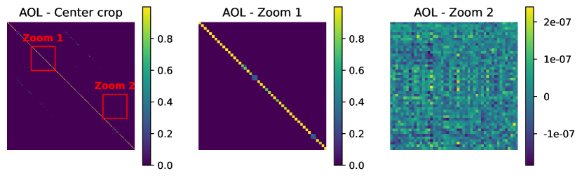
Figure 1: Evaluation of the orthogonality of the trained model. We consider the third layer of the AOL-Small model. It is a $3\times 3$ convolutions with input size $8\times 8\times 192$. We show a center crop of $J^{\top}J$, for $J$ the Jacobian, as well as two further crops. Note that most diagonal elements are close to $1$, and most off-diagonal elements are very close to $0$ (note the different color scale in the third subplot). This confirms that AOL did indeed learn an almost-orthogonal weight matrix. Best viewed in color and zoomed in.

Table 5: Experimental results for AOL-Small for different value of $u$ and $t$ in the loss function in Equation (10). We report the standard accuracy on the test set as well as the certified robust accuracy under input perturbations up to size $\epsilon$ for different values of $\epsilon$.

$u$	$t$	Standard	Certified robust accuracy
		Accuracy	$\epsilon=\frac{36}{255}$	$\epsilon=\frac{72}{255}$	$\epsilon=\frac{108}{255}$	$\epsilon=1$
$\sqrt{2}/16$	$1/64$	79.8%	45.3%	16.7%	3.3%	0.0%
$\sqrt{2}/4$	$1/16$	77.4%	63.0%	47.6%	33.0%	2.5%
$\sqrt{2}$	$1/4$	70.4%	62.6%	55.0%	47.9%	22.2%
$4\sqrt{2}$	$1$	59.8%	55.5%	50.9%	46.5%	30.8%
$16\sqrt{2}$	$4$	48.2%	45.2%	42.2%	39.4%	28.6%

Accuracy-Robustness Tradeoff: The loss function in Equation (10) allows trading off between clean accuracy and certified robust accuracy by changing the size of the enforced margin. We demonstrate this by an ablation study that varies the offset parameter $u$ in the loss function, and also scales $t$ proportional to $u$.

The results can be found in Table 5. One can see that using a small margin allows us to train an AOL Network with high clean accuracy, but decreases the certified robust accuracy for larger input perturbations, whereas choosing a higher offset allows us to reach state-of-the-art accuracy for larger input perturbations. Therefore, varying this offset gives us an easy way to prioritize the measure that is important for a specific problem.

7 Conclusion

In this work, we proposed AOL, a method for constructing deep networks that have Lipschitz constant of at most $1$ and therefore are robust against small changes in the input data. Our main contribution is a rescaling technique for network layers that ensures them to be 1-Lipschitz. It can be computed and trained efficiently, and is applicable to fully-connected and various types of convolutional layers. Training with the rescaled layers leads to weight matrices that are almost orthogonal without the need for a special parametrization and computationally costly orthogonalization schemes. We present experiments and ablation studies in the context of image classification with certified robustness. They show that AOL-networks achieve results comparable with methods that explicitly enforce orthogonalization, while offering the simplicity and flexibility of earlier bound-based approaches.

Appendix A Appendix

A.1 Proof of Lemma 4.2

We will proof the Lemma 4.2 here. Recall

*

Proof.

For the proof we will assume maximal padding of the input: We pad an input $x\in\mathbb{R}^{n\times n\times c_{\text{I}}}$ (with values independent of $x$) to a size of $(n+2k-2)\times(n+2k-2)\times c_{\text{I}}$, and then apply the convolution to the padded input. Then we obtain an output of size $(n+k-1)\times(n+k-1)\times c_{\text{O}}$. We will derive a rescaling of the input that ensures this convolution has a Lipschitz constant of $1$. Then, any convolution with a different kind of padding (such as same size or valid) can be considered as first doing a maximally padded convolution, followed by a center cropping operation. Since a cropping operation also has a Lipschitz constant of $1$, this also shows that convolutional layers with a different kind of padding have a Lipschitz constant of $1$.

Denote by $\tilde{x}$ the padded version of input $x$, with $\tilde{x}_{i+k-1,j+k-1}=x_{i,j}$. Then, the multi-channel, maximally padded convolution with a convolutional kernel $P\in\mathbb{R}^{k\times k\times c_{I}\times c_{O}}$ is given by

$$[P*x]^{b}_{i,j}=\sum_{p=0}^{k-1}\sum_{q=0}^{k-1}\sum_{a=1}^{c_{I}}P^{(a,b)}_{p,q}\tilde{x}^{a}_{i+p,j+q},$$ (11)

for $1\leq i,j\leq n+k-1$ and $1\leq b\leq c_{\text{O}}$.

We now consider the Jacobian $J$ of the linear map (from unpadded input to output) defined by Equation 11. It is a matrix of size $(n+k-1)^{2}c_{\text{O}}\times n^{2}c_{\text{I}}$, with entries given by

$$J^{(b,a)}_{(i_{2},j_{2}),(i_{1},j_{1})}=P^{(a,b)}_{(i_{1}-i_{2}+k-1),(j_{1}-j_{2}+k-1)},$$ (12)

for $1\leq i_{1},i_{2}\leq n$, $1\leq i_{2},j_{2}\leq n+k-1$, $1\leq a\leq c_{\text{I}}$ and $1\leq b\leq c_{\text{O}}$. Here, we define $P^{(a,b)}_{p,q}=0$ unless $0\leq p<n$ and $0\leq q<n$.

We can use that to obtain an expression for $J^{\top}J$ (writing $m=n+k-1$):

$$[J^{\top}J]^{(a_{1},a_{2})}_{(i_{1},j_{1}),(i_{2},j_{2})}$$ (13)

$$\qquad=\sum_{i=1}^{m}\sum_{j=1}^{m}\sum_{b=1}^{c_{\text{O}}}J^{(b,a_{1})}_{(i,j),(i_{1},j_{1})}J^{(b,a_{2})}_{(i,j),(i_{2},j_{2})}$$ (14)

$$\qquad=\sum_{i=1}^{m}\sum_{j=1}^{m}\sum_{b=1}^{c_{\text{O}}}P^{(a_{1},b)}_{(i_{1}-i+k-1),(j_{1}-j+k-1)}P^{(a_{2},b)}_{(i_{2}-i+k-1),(j_{2}-j+k-1)}$$ (15)

$$\qquad=\sum_{i=0}^{k-1}\sum_{j=0}^{k-1}\sum_{b=1}^{c_{\text{O}}}P^{(a_{1},b)}_{i,j}P^{(a_{2},b)}_{(i+i_{2}-i_{1}),(j+j_{2}-j_{1})}$$ (16)

$$\qquad=\left(\sum_{b=1}^{c_{\text{O}}}P^{(a_{1},b)}*P^{(a_{2},b)}\right)_{i_{2}-i_{1},j_{2}-j_{1}}.$$ (17)

We can now apply Theorem 1 (from the main paper) with $P=J$ together with Equation (17) in order to obtain the necessary rescaling: In order to guarantee the convolution to have Lipschitz constant $1$, we need to multiply input $x^{(c)}_{i_{2},j_{2}}$ by

$$\left(\sum_{i_{1}=1}^{n}\sum_{j_{1}=1}^{n}\sum_{a_{1}=1}^{c_{\text{I}}}\left|\sum_{b=1}^{c_{\text{O}}}P^{(a_{1},b)}*P^{(c,b)}\right|_{i_{2}-i_{1},j_{2}-j_{1}}\right)^{-1/2}.$$ (18)

A lower bound of this expression (that is tight for most values of $i_{2}$ and $j_{2}$) is given by

$$\left(\sum_{i=-k+1}^{k}\sum_{j=-k+1}^{k}\sum_{a=1}^{c_{\text{I}}}\left|\sum_{b=1}^{c_{\text{O}}}P^{(a,b)}*P^{(c,b)}\right|_{i,j}\right)^{-1/2}.$$ (19)

This value is independent of both $i_{2}$ and $j_{2}$, so this completes our proof for maximally padded convolutions. This also implies that convolutions with less padding have a Lipschitz constant of $1$ when the input is rescaled as described. ∎∎

Note that this proof requires padding independent of the input. However, for example for cyclic padding, the Jacobian is a doubly circuland matrix, and a very similar proof shows that our rescaling still works.

Also note that a result similar to equation (17), relating $J^{\top}J$ to a self-convolution, has been observed before by [10].

A.2 Comparison of the orthogonality

We will present a comparison of $J^{\top}J$ for $J$ the Jacobian of different layers. We consider three architectures: A standard convolutional architecture with standard convolutions (see Section A.4.1), the same architectures with AOL convolutions and (theoretically) an architecture with perfectly orthogonal Jacobian. We pick the third layer of this architecture. It is a convolution with kernel of size $3\times 3\times 32\times 32$, and input as well as output of size $32\times 32\times 32$. This results in a Jacobian $J$ of size $32\,768\times 32\,768$, and we calculate and visualize the values of a center crop of size $288\times 288$ of the matrix $J^{\top}J$. (See Figure 2.)

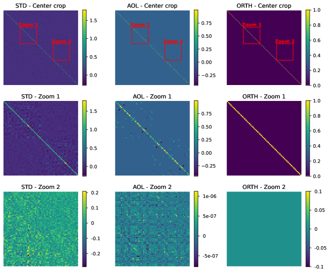
Figure 2: Evaluation of orthogonality of trained models. The first row shows a center crop of $J^{\top}J$, where $J$ is the Jacobian of the layer, as well as the location of the other two crops. Those are shown in the second and third row. Left column: Standard convolutional layer (STD). Center column: AOL-STD (AOL), Right column: (Perfectly) orthogonal layer (ORTH). Note the different color scales of different subplots. Best viewed in color and zoomed in.

One can see that for our AOL-STD architecture most off-diagonal elements are very close to $0$, whereas for the standard architecture they are not. Interestingly, for our architecture there are some off-diagonal elements that are clearly non-zero. This shows that the learning resulted in a few column pairs not being orthogonal, in line with our claim of almost-orthogonality.

A.3 Accuracies of different architectures

The results for different architectures using our proposed AOL layers are in Table 6.

Table 6: Experimental results for different architectures using AOL on CIFAR-10. We report the standard accuracy on the test set as well as the certified robust accuracy under input perturbations up to size $\epsilon$ for different values of $\epsilon$.

Method	Standard	Certified Robust Accuracy
	Accuracy	$\epsilon=\frac{36}{255}$	$\epsilon=\frac{72}{255}$	$\epsilon=\frac{108}{255}$	$\epsilon=1$
AOL-FC	67.9%	59.1%	51.1%	43.1%	17.6%
AOL-STD	65.0%	56.4%	48.2%	39.9%	15.8%
AOL-ALT	68.4%	60.3%	52.4%	44.8%	19.9%
AOL-DIL	62.7%	54.2%	46.0%	38.3%	14.9%

A.4 Further Architectures

We present the other architectures here that were used in the ablation studies.

A.4.1 Standard CNN:

In this Architecture the number of channels doubles whenever the spatial size is decreased. For details see Table 7.

Table 7: A relatively standard convolutional architecture for CIFAR-10. For all layers we use zero padding to keep the size the same. First channels just selects the first channels and ignores the rest.

Layer name	Filters	Kernel size	Stride	Activation	Output size	Amount
Conv	$32$	$3\times 3$	$1\times 1$	MaxMin	$32\times 32\times 32$	$4$
Conv	$64$	$2\times 2$	$2\times 2$	None	$16\times 16\times 64$	$1$
Conv	$64$	$3\times 3$	$1\times 1$	MaxMin	$16\times 16\times 64$	$4$
Conv	$128$	$2\times 2$	$2\times 2$	None	$8\times 8\times 128$	$1$
Conv	$128$	$3\times 3$	$1\times 1$	MaxMin	$8\times 8\times 128$	$4$
Conv	$256$	$2\times 2$	$2\times 2$	None	$4\times 4\times 256$	$1$
Conv	$256$	$3\times 3$	$1\times 1$	MaxMin	$4\times 4\times 256$	$4$
Conv	$512$	$2\times 2$	$2\times 2$	None	$2\times 2\times 512$	$1$
Conv	$512$	$3\times 3$	$1\times 1$	MaxMin	$2\times 2\times 512$	$4$
Conv	$1024$	$2\times 2$	$2\times 2$	None	$1\times 1\times 1024$	$1$
Conv	$1024$	$1\times 1$	$1\times 1$	None	$1\times 1\times 1024$	$1$
First Channels	-	-	-	-	$1\times 1\times 10$	$1$
Flatten	-	-	-	-	$10$	$1$

A.4.2 AOL-FC:

Architecture consisting of $9$ fully connected layers. For details see Table 8.

Table 8: Fully Connected Architecture. First channels just selects the first channels and ignores the rest.

Layer name	Activation	Output size	Amount
Flatten	-	3072	$1$
AOL FC	MaxMin	4096	$8$
AOL FC	None	4096	$1$
First Channels	-	$10$	$1$

A.4.3 AOL-STD:

This architecture is identical to the one in Table 7, only with standard convolutions replaced by AOL convolutions.

A.4.4 AOL-ALT:

Architecture that quadruples the number of channels whenever the spatial size is decreased in order to keep the number of activations constant for the first few layers. This is done until there are $1024$ channels, then the number of channels is kept at this value. For details see Table 9.

Table 9: Convolutional architecture. For all layers we use zero padding to keep the size the same. First channels just selects the first channels and ignores the rest.

Layer name	Filters	Kernel size	Stride	Activation	Output size	Amount
AOL Conv	$16$	$2\times 2$	$2\times 2$	MaxMin	$16\times 16\times 16$	$1$
AOL Conv	$16$	$3\times 3$	$1\times 1$	MaxMin	$16\times 16\times 16$	$4$
AOL Conv	$64$	$2\times 2$	$2\times 2$	MaxMin	$8\times 8\times 64$	$1$
AOL Conv	$64$	$3\times 3$	$1\times 1$	MaxMin	$8\times 8\times 64$	$4$
AOL Conv	$256$	$2\times 2$	$2\times 2$	MaxMin	$4\times 4\times 256$	$1$
AOL Conv	$256$	$3\times 3$	$1\times 1$	MaxMin	$4\times 4\times 256$	$4$
AOL Conv	$1024$	$2\times 2$	$2\times 2$	MaxMin	$2\times 2\times 1024$	$1$
AOL Conv	$1024$	$1\times 1$	$1\times 1$	MaxMin	$2\times 2\times 1024$	$4$
AOL Conv	$1024$	$1\times 1$	$1\times 1$	None	$2\times 2\times 1024$	$1$
First Channels	$256$	-	-	-	$2\times 2\times 256$	$1$
AOL Conv	$1024$	$2\times 2$	$2\times 2$	MaxMin	$1\times 1\times 1024$	$1$
AOL Conv	$1024$	$1\times 1$	$1\times 1$	MaxMin	$1\times 1\times 1024$	$4$
AOL Conv	$1024$	$1\times 1$	$1\times 1$	None	$1\times 1\times 1024$	$1$
First Channels	$10$	-	-	-	$1\times 1\times 10$	$1$
Flatten	-	-	-	-	$10$	$1$

A.4.5 AOL-DIL

We use an architecture similar to the one used by ECO. For that, we just replace each $3\times 3$ convolution in the architecture in Table 7 with a strided AOL convolution.

A.5 Data augmentation

We use data augmentation in all our experiments. We first do some color augmentation of the images, followed by some spatial transformations. For the color augmentation, we first adjust the hue of the image (by a random factor with delta in $[-0.02,0.02]$), then we adjust the saturation of the image (by a factor in $[.3,2]$), then we adjust the brightness of the image (by a random factor with delta in $[-0.1,0.1]$), and finally we adjust the contrast of the image (by a factor in $[.5,2]$). After this we clip the pixel values so they are in $[0.,1.]$. For the spatial transformations, we first apply a random rotation, with a maximal rotation of $5$ degrees. Then we apply a random shift of up to $10\%$ of the image size, and finally we flip the image with a probability of $50\%$. We rely on the tensorflow layers RandomRotation and RandomTranslation for the spatial transformations, and leave all hyperparameters such as the fill mode as the default values. All hyperparameters specifying the amount of augmentation were chosen based on visual inspection of the augmented training images.

References

- [1] Christian Szegedy, Wojciech Zaremba, Ilya Sutskever, Joan Bruna, Dumitru Erhan, Ian J. Goodfellow, and Rob Fergus. Intriguing properties of neural networks. In International Conference on Learning Representations (ICLR), 2014.
- [2] Anirban Chakraborty, Manaar Alam, Vishal Dey, Anupam Chattopadhyay, and Debdeep Mukhopadhyay. Adversarial attacks and defences: A survey. arXiv preprint arXiv:1810.00069, 2018.
- [3] Alex Serban, Erik Poll, and Joost Visser. Adversarial examples on object recognition: A comprehensive survey. ACM Computing Surveys (CSUR), 53(3):1–38, 2020.
- [4] Han Xu, Yao Ma, Hao-Chen Liu, Debayan Deb, Hui Liu, Ji-Liang Tang, and Anil K Jain. Adversarial attacks and defenses in images, graphs and text: A review. International Journal of Automation and Computing, 17(2):151–178, 2020.
- [5] Aladin Virmaux and Kevin Scaman. Lipschitz regularity of deep neural networks: analysis and efficient estimation. In Conference on Neural Information Processing Systems (NeurIPS), 2018.
- [6] Martin Arjovsky, Soumith Chintala, and Léon Bottou. Wasserstein generative adversarial networks. In International Conference on Machine Learing (ICML), 2017.
- [7] Ishaan Gulrajani, Faruk Ahmed, Martin Arjovsky, Vincent Dumoulin, and Aaron C Courville. Improved training of Wasserstein GANs. In Conference on Neural Information Processing Systems (NeurIPS), 2017.
- [8] Takeru Miyato, Toshiki Kataoka, Masanori Koyama, and Yuichi Yoshida. Spectral normalization for generative adversarial networks. In International Conference on Learning Representations (ICLR), 2018.
- [9] Moustapha Cissé, Piotr Bojanowski, Edouard Grave, Yann N. Dauphin, and Nicolas Usunier. Parseval networks: Improving robustness to adversarial examples. In International Conference on Machine Learing (ICML), 2017.
- [10] Jiayun Wang, Yubei Chen, Rudrasis Chakraborty, and Stella X. Yu. Orthogonal convolutional neural networks. In Conference on Computer Vision and Pattern Recognition (CVPR), 2020.
- [11] Henry Gouk, Eibe Frank, Bernhard Pfahringer, and Michael J Cree. Regularisation of neural networks by enforcing Lipschitz continuity. Machine Learning, 110(2):393–416, 2021.
- [12] Yusuke Tsuzuku, Issei Sato, and Masashi Sugiyama. Lipschitz-margin training: Scalable certification of perturbation invariance for deep neural networks. In Conference on Neural Information Processing Systems (NeurIPS), 2018.
- [13] Klas Leino, Zifan Wang, and Matt Fredrikson. Globally-robust neural networks. In International Conference on Machine Learing (ICML), 2021.
- [14] Bai Li, Changyou Chen, Wenlin Wang, and Lawrence Carin. Certified adversarial robustness with additive noise. In Conference on Neural Information Processing Systems (NeurIPS), 2019.
- [15] Cem Anil, James Lucas, and Roger B. Grosse. Sorting out Lipschitz function approximation. In International Conference on Machine Learing (ICML), 2019.
- [16] Lei Huang, Li Liu, Fan Zhu, Diwen Wan, Zehuan Yuan, Bo Li, and Ling Shao. Controllable orthogonalization in training DNNs. In Conference on Computer Vision and Pattern Recognition (CVPR), 2020.
- [17] Asher Trockman and J. Zico Kolter. Orthogonalizing convolutional layers with the Cayley transform. In International Conference on Learning Representations (ICLR), 2021.
- [18] Sahil Singla and Soheil Feizi. Skew orthogonal convolutions. In International Conference on Machine Learing (ICML), 2021.
- [19] Tan Yu, Jun Li, YUNFENG CAI, and Ping Li. Constructing orthogonal convolutions in an explicit manner. In International Conference on Learning Representations (ICLR), 2022. (to appear).
- [20] Å. Björck and C. Bowie. An iterative algorithm for computing the best estimate of an orthogonal matrix. SIAM Journal on Numerical Analysis, 1971.
- [21] Arthur Cayley. About the algebraic structure of the orthogonal group and the other classical groups in a field of characteristic zero or a prime characteristic. Journal für die reine und angewandte Mathematik, 1846.
- [22] Hanie Sedghi, Vineet Gupta, and Philip M. Long. The singular values of convolutional layers. In International Conference on Learning Representations (ICLR), 2019.
- [23] Asher Trockman and J Zico Kolter. Patches are all you need? arXiv preprint arXiv:2201.09792, 2022.
- [24] Artem N. Chernodub and Dimitri Nowicki. Norm-preserving orthogonal permutation linear unit activation functions (oplu). CoRR, 2016.
- [25] Sahil Singla, Surbhi Singla, and Soheil Feizi. Improved deterministic robustness on CIFAR-10 and CIFAR-100. In International Conference on Learning Representations (ICLR), 2022. (to appear).