A Lightweight Machine Learning Pipeline for LiDAR-simulation

Abstract

Virtual testing is a crucial task to ensure safety in autonomous driving, and sensor simulation is an important task in this domain. Most current LiDAR simulations are very simplistic and are mainly used to perform initial tests, while the majority of insights are gathered on the road. In this paper, we propose a lightweight approach for more realistic LiDAR simulation that learns a real sensor’s behavior from test drive data and transforms this to the virtual domain. The central idea is to cast the simulation into an image-to-image translation problem. We train our pix2pix based architecture on two real world data sets, namely the popular KITTI data set and the Audi Autonomous Driving Dataset which provide both, RGB and LiDAR images. We apply this network on synthetic renderings and show that it generalizes sufficiently from real images to simulated images. This strategy enables to skip the sensor-specific, expensive and complex LiDAR physics simulation in our synthetic world and avoids oversimplification and a large domain-gap through the clean synthetic environment.

1 INTRODUCTION

Even though Autonomous Driving (AD) and Advanced Driver Assistance Systems (ADAS) have been a major research areas for more than a decade, the adoption into practical driving systems is dragging on. With the lacking capabilities of current algorithms to adapt to unforeseen situations, a big challenge is testing the performance of such systems safely. A key part to achieve this vision is the realistic simulation of the car sensors such as cameras, LiDAR or RADAR. Simulating such sensors in a virtual environment is costly, in particular if the virtual sensors should suffer from the same physical limitations and imperfections as their real counterpart.

A typical approach are physical based simulations, which require extensive data about the sensor specifics and a careful implementation. A more desirable option is to learn the behavior of a particular sensor from recorded real test drive data and to transfer this to a virtual sensor. The process should be mostly automatic, in order to easily adapt the simulation to new models and types of sensors.

The core idea of this paper is to tackle the problem as an image-to-image translation task. In particular, we consider the simulation of LiDAR sensors, which send out light beams in a uniform cylindrical grid and measure the time of flight and thus the distance of the scene point visible in this particular direction. If there is no hit point (sky), the hit point absorbs the light (dark surfaces), or does not reflect back (mirroring surface) or multiple reflections interfere, no measurement is returned. Of course, the possibilities to learn sensor behavior strongly depend on the available test drive (and thus ground truth data).

Relevant for our purpose are a RGB camera stream and a synchronized stream of LiDAR points. Our concept is shown in Fig. 1: from recorded test drive data, we learn the transfer from RGB camera images to LiDAR images using the Pix2Pix architecture [Isola et al., 2018].

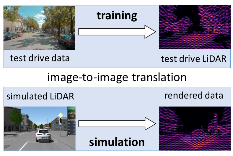
Figure 1: We learn the translation from real world RGB to LiDAR data from test drives. We use this learned mapping to derive LiDAR output from rendered RGB images.

Fig. 1 already shows a potential challenge of the approach: real and simulated RGB images still have significantly different characteristics. It is unclear, how much this gap between real and simulated imagery influences the outcome in the simulation. We thus examine other input image types, e.g. depth images, or segmentation images, where the real-2-sim gap might be smaller.

In this study, we explore variants of this idea and show that it is possible to learn a plausible LiDAR simulation solely from test drive data, in our case KITTI and A2D2. Our simulation runs in real-time and can thus be integrated in a virtual test drive system. We compare the different modalities of input images and ablate which are most suitable for our learned LiDAR simulation strategy. We evaluate our idea by examining how well ground truth LiDAR data can be reproduced with our approach, and how well we can predict real LiDAR measurements from synthetic rendered data using the second revision [Cabon et al., 2020] of the Virtual KITTI data set (VKITTI).

2 RELATED WORK

Simulation Environments

Many modern simulation environments like LGSVL [LG, 2021], CARLA [Dosovitskiy et al., 2017] or Intel Airsim [Shah et al., 2017] build on game engines to offer high quality graphics and profit from their development and communities. Additionally, there are different ADAS integrations, sensor configurations and simulation settings, e.g. weather or traffic, to support many use cases of automotive simulation. Other tools like VTD [VTD, 2021] or IPG Carmaker [Automotive, 2020] focus on supporting their own software stack and promise a more complete solution.

These environments also offer sensor simulations. Yet, existing LiDAR simulations are usually simplistic and not sufficient to test ADAS or autonomous vehicles, so we see potential for our approach here. To integrate our approach into these systems, we only need to get access to rendered RGB images, their depth buffer, or segmentation masks, so the integration of a new module that transfers these images to LiDAR sensor output is very simple.

Nvidia DRIVE Sim [NVIDIA, 2021] is different in this regard, as it builds on the direct cooperation with LiDAR companies to offer better integrations. However, while there exist relatively realistic physics based simulations, these are locked into the Nvidia ecosystem, so we see them as rather complementary to our accessible data based approach.

Furthermore, our approach makes it possible to learn the behavior of new LiDAR sensor boxes only based on test drive data, without knowing or tuning the internal physical parameters.

Data Sets

Many high quality data sets from test drives have emerged in recent years [Sun et al., 2020] [Uhrig et al., 2017] and the trend continues [Liao et al., 2021]. LiDAR data is very common to be included in these data sets, which makes them compatible with our approach. The usual representation format are LiDAR point clouds. For each such point, there is a position, an intensity value and a time stamp. Using the sensor orientation and offset between the RGB camera, it is possible to compute a 2D LiDAR projection. Often, this format is already included in the data sets directly or the necessary projection matrices are given. Notably, [Gaidon et al., 2016, Cabon et al., 2020] replicates KITTI scenes virtually with a semi-manual process, thereby providing ground truth data like depth and semantic segmentation. This allows us to compare how well our trained network is able to generalize between synthetic and real data on the same driving data sequences.

Image-to-image Translation

In a way, the 2D LiDAR projection can be interpreted as a special segmentation of the RGB image using two classes: visible by the LiDAR sensor and not visible. Consequently, the popular U-Net architecture [Ronneberger et al., 2015], using an encoder network, followed by a decoder network, immediately suggests itself. However, to simulate the actual LiDAR pattern in the projection, it is also important that unrealistic outputs are penalized. This can be achieved efficiently with General Adversarial Networks (GANs) [Goodfellow et al., 2014], where a discriminator is optimized that estimates whether an image is fake or not. Pix2pix [Isola et al., 2018] combines the strength of U-Nets and an adversarial loss and demonstrated success for very diverse image domains. There are also approaches that perform this task in an unpaired fashion [Zhu et al., 2020], but for the pipeline proposed in this paper, we can assume that paired images exist.

Building on pix2pix, pix2pixHD [Wang et al., 2018a] and SPADE [Park et al., 2019] have improved the quality of results via adapting the architecture more towards specific data domains.An alternative would be the direction of style transfer [Johnson et al., 2016]. Following this approach, one could use an average LiDAR projection and apply it to different images. Given the available data, which offers a specific LiDAR projection for each individual input image, image-to-image translation is a better fit for our purposes.

Learning based Sensor Simulation

A very interesting approach for LiDAR simulation is pseudo-LiDAR [Wang et al., 2018b]. It is similar in regard to how point clouds are generated based on RGB images and depth prediction networks. However, the end goal of this method is to improve image based object detection, while our pipeline is more general and generates realistic LiDAR data on purpose as an intermediate representation to be used to train various downstream applications.

On a conceptual level, we pursue the same approach as L2R GAN [Wang et al., 2020], but try to learn the mapping between camera images and camera LiDAR projections instead of the one between bird’s eye view LiDAR and radar images.

The closest approach to ours is LiDARsim [Manivasagam et al., 2020]. It also aims at realistic simulation of LiDAR leveraging real world data but use a physics based light simulation as foundation. To obtain realistic geometry, a virtual copy is reconstructed by merging multiple scans from test drives. Instead of directly predicting the LiDAR point distribution based on camera images, LiDARsim first uses ray casting in this virtual scene to create a perfect point cloud. Based on these and the LiDAR scans from the test data, the network then learns to drop rays from the ray casted point clouds for enhanced realism.

With our method, we try to achieve a more lightweight LiDAR simulation for situations where such preprocessing is not feasible. For direct integration into external simulation environments, a solution is required that does not dependend on high quality geometry data.

3 TRAINING AND SIMULATION

3.1 LiDAR Images

To learn and simulate the behaviour of LiDAR sensors, we map our problem to an image-to-image translation task. Therefore, we convert the LiDAR output to an image which we call LiDAR image. We notice that the problem of LiDAR simulation in a virtual environment is not the measured distance of a particular sample, as this can easily be determined by ray casting. Instead, we need to decide which LiDAR rays return an answer and which do not, e.g. due to absorption, specular reflection, or diffusion. We map this information to a LiDAR image, that tells us for a particular view direction, whether a ray in this direction is likely to return an answer.

To this end, we project the LiDAR point cloud into the camera view, which requires that we know the relative pose of LiDAR and camera and that the outputs of all devices are aligned temporally and have a timestamp. An example is shown in Fig. 2(b). The binary image shows, which regions are visible for the sensor, but also which problems arise when trying to predict them: Since camera and LiDAR sensor usually do not have the same optical center, the position of the projection varies with depth. A network has to predict depth implicitly to output dots at the proper position.

We thus blur the binary image with a simple Gaussian filter, as shown in Fig. 2(c), Note that we color coded the result for better visualization. The resulting map is denser, so (i) it better abstracts from the exact sample positions and (ii) the map is easier to predict. The size of the Gaussian filter is chosen such that gaps between neighboring dots are filled, but also such that invisible regions are not filled up wrongly. It depends on the scan pattern of the LiDAR and the image resolution, which we choose in turn depending on the horizontal and vertical distribution. In our examples, we use a Gaussian blur with $\sigma=8$ to make up for the sparsity in the A2D2 data set (image resolution $1920\times 1208$) and a rather small intervention for KITTI (image resolution $1242\times 375$), only using a small 5x5 custom kernel as shown in Fig. 2(c). There are also more elaborate ways of augmenting the data [Shorten and Khoshgoftaar, 2019], but the basic blurring we use is well suited for LiDAR data and resulted in a sufficient improvement of the training results.

The blurring also helps to hide another, more subtle inconsistency: usually, the camera frame rate is higher than that of the LiDAR. However, to get a full LiDAR pattern, we project all points from a single complete LiDAR scan to each camera frame. Additionally, each LiDAR sample comes from another time interval, resulting in a rolling shutter effect. By blurring and interpolating all this, we achieve a less sharp, but more consistent visibility mask. The LiDAR image also contains information about the scan pattern of the LiDAR, and can even be used to represent the result of multiple LiDAR sensors, as in the A2D2 dataset shown in Fig. 2(d).

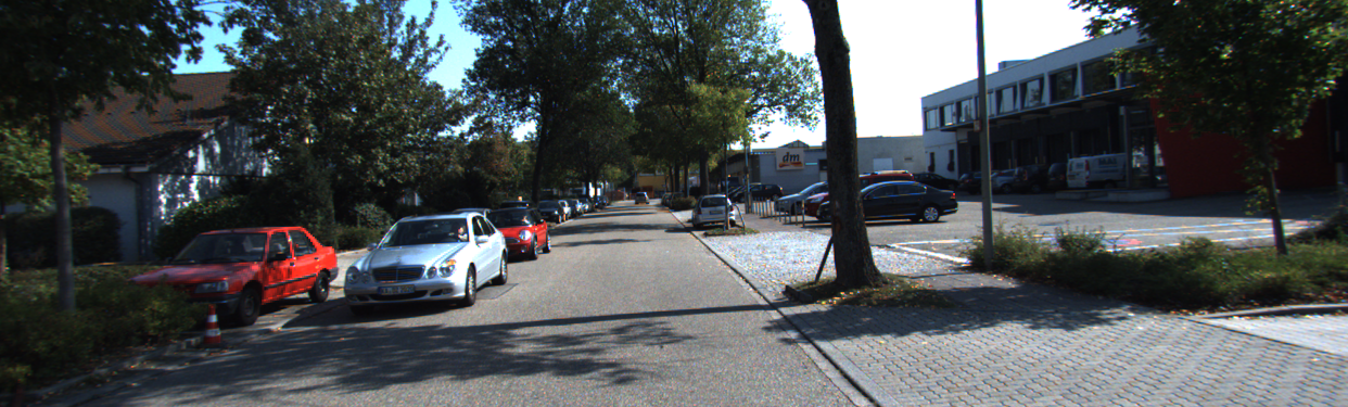
(a) RGB image from the KITTI data set.

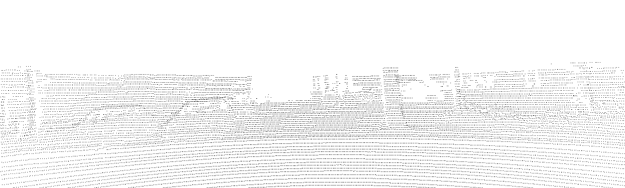
(b) LiDAR points projected into same view.

(c) Blurred and color coded LiDAR image.

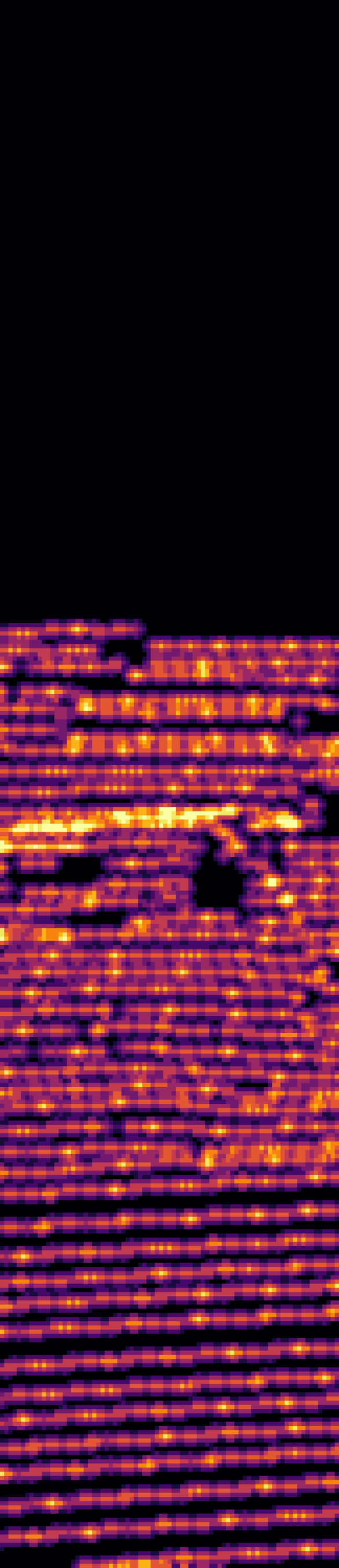
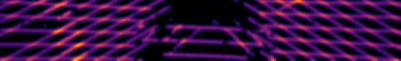
(d) LiDAR images from two different data sets (left: KITTI, right: A2D2 with five sensors resulting in a grid pattern)

Figure 2: LiDAR image generation

3.2 LiDAR Simulation

Our hypothesis is that an image-to-image translation of an RGB image to a LiDAR image should be well possible, since in an RGB image it is possible to detect LiDAR-critical regions, such as sky, far distances, or transparent/mirroring surfaces (e.g., windows). However, it is unclear how well the network trained on real data generalizes to rendered and thus much cleaner images.

We furthermore hypothesize that a translation to LiDAR images is also possible from depth images or from segmentation images. Such images are very simple to generate in a driving simulation, however these are not generally available as ground truth data for training and thus have to be derived (e.g. using depth estimation networks), or generated manually (e.g. segmentation masks).

In the following, we explore all these options, see Fig. 3. In particular, we describe how to generate the input data, how our image-to-image transformation is done, and how we integrated all this into a virtual test environment.

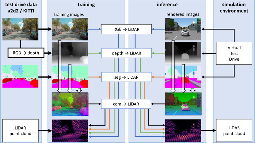
Figure 3: Overview over training and inference of our LiDAR simulation. We explore prediction of LiDAR point clouds based on RGB, depth and segmentation images separately and combined. We train on real RGB and LiDAR pairs and apply the learned mapping on rendered image to synthesize realistic LiDAR images.

3.3 Training Data

We use two data sets to generate our training data:

• KITTI: We use the training set [Weber et al., 2021] from the Segmenting and Tracking Every Pixel Evaluation benchmark, since it also includes segmentation data. We make a slight variation to the validation set and only include the sequences that are present in VKITTI. This results in roughly 6000 training and 2000 validation images

• A2D2: We leave about 20000 images for training and create a validation set from three different test drives, one in a urban setting, one on a highway and one on a country road making up 6000 images. In contrast to many other data sets, A2D2 uses five low resolution LiDAR sensors in tandem to achieve sufficient point density.

The KITTI and A2D2 dataset create different LiDAR patterns, which allows us to test our approach on different point layouts (see Fig. 2d). Our learning based approach overcomes the need to implement the physics of each sensor for implementation and enables to learn the sensor properties for a simulated environment.

As input to our image-to-image network we consider RGB camera images, depth images, and/or segmentation masks. Ground truth depth maps are usually not available, so we derive them using mono depth estimation [Ranftl et al., 2021]. If ground truth segmentation masks are not available, they can be estimated using segmentation networks, e.g. [Ranftl et al., 2021, Kirillov et al., 2019]. As forth option, we combine camera, depth, and segmentation images by merging a grey scale version of the camera image, depth, and segmentation label. To avoid the use of the same value for different semantic objects, the colors of the class labels are mapped to specific grey values. Overall, we follow the set of more than 50 different classes defined by A2D2. The color encoding also includes instance segmentation of up to four instances per class so that overlapping objects can be discerned.

3.4 Image-to-image Translation

Many different network architectures for image-to-image translation have been presented, our experiments have shown that pix2pix and even simpler encoder-decoder architectures like U-Nets [Ronneberger et al., 2015] deliver satisfying results as also shown by LiDARsim [Manivasagam et al., 2020]. We apply a widely used implementation which is based on a U-Net architecture and a convolutional PatchGAN classifier as proposed in the original pix2pix paper [Isola et al., 2018]. We leave the network architecture unchanged but omit the preprocessing step that crops and flips the pictures randomly. This step is problematic for LiDAR projections as they are dependent on the camera perspective and not necessarily symmetric.

Our experiments have shown that deviations in the basic parameters of the architecture only show little effect. For the presented results we used the following configuration: Adam optimizer with learning rate of $2*10^{-4}$ and $\beta_{1}=0.5$ and $\lambda=100$ for computing $\text{Generator Loss}=\text{Adversarial Loss}+\lambda*\text{L1 Loss}$.

3.5 Integration

Once training is completed, we integrate the learned LiDAR sensor network into our simulation environment and our network then predicts a LiDAR image, as shown in Fig. 3. To convert back to a LiDAR point cloud, a simple approach is to sample the map directly: (i) sample the visibility map, e.g. on a uniform grid, (ii) discard all points with small visibility, (iii) determine the remaining samples’ depth from the depth map, (iv) reproject the points into a 3D coordinate space.

The resulting point cloud mimics the behavior of the real sensor, in particular typically invisible points are missing, but the original LiDAR pattern is probably not represented well.

A more expensive, but also more precise solution is to generate virtual rays for the original LiDAR samples, compute their hit point by ray casting, and check the visibility of the hit point in the predicted LiDAR visibility map. This approach can also consider the car movement during a LiDAR scan and thus reproduce the rolling shutter effect.

4 EXPERIMENTS AND RESULTS

Overall, our implementation achieves a visually reasonable mapping between input image and LiDAR projection. The training on the data translates well to the test data sets and also generalizes on synthetic data to a sufficient degree.

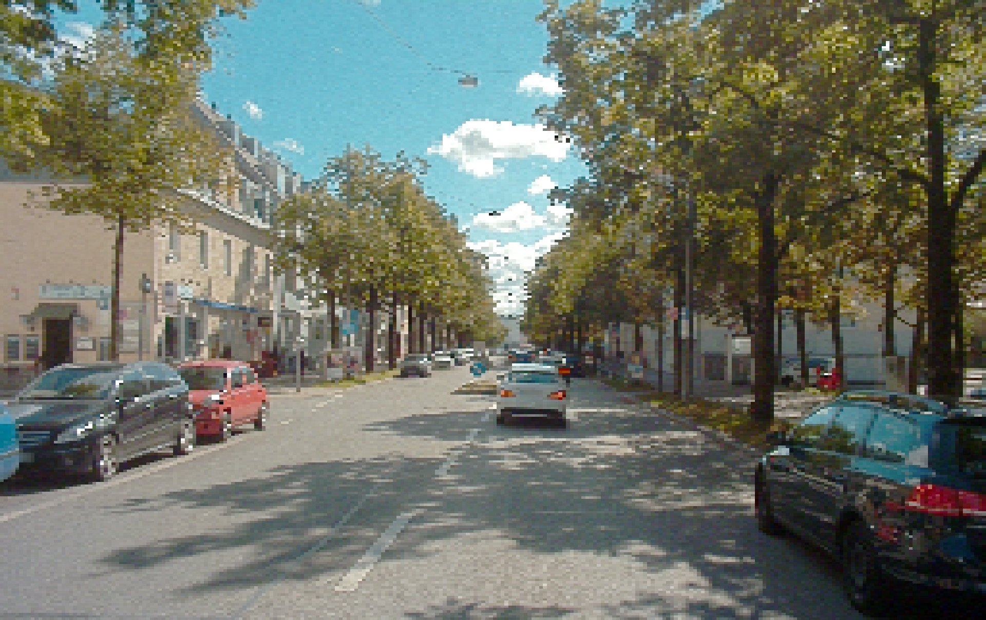
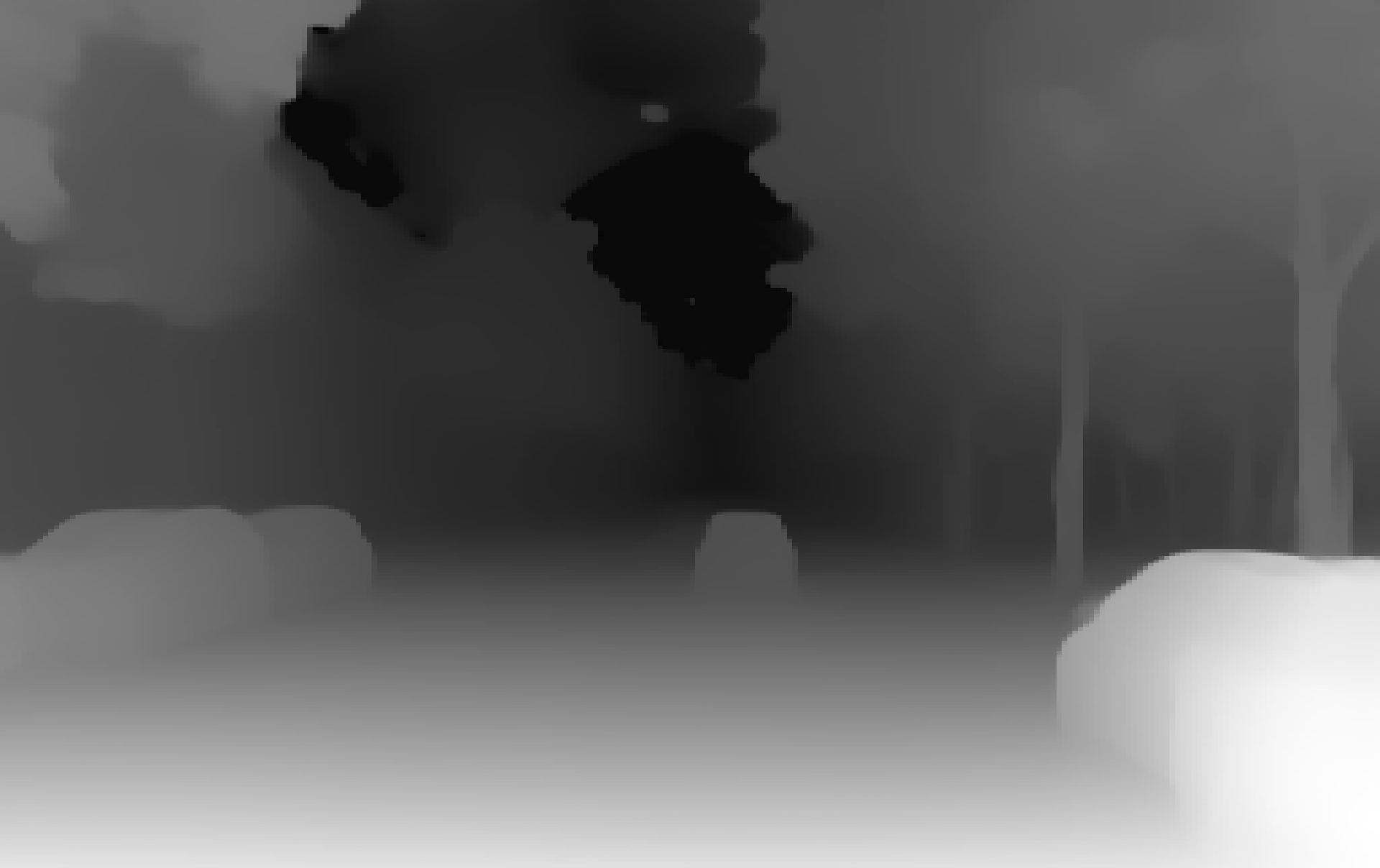
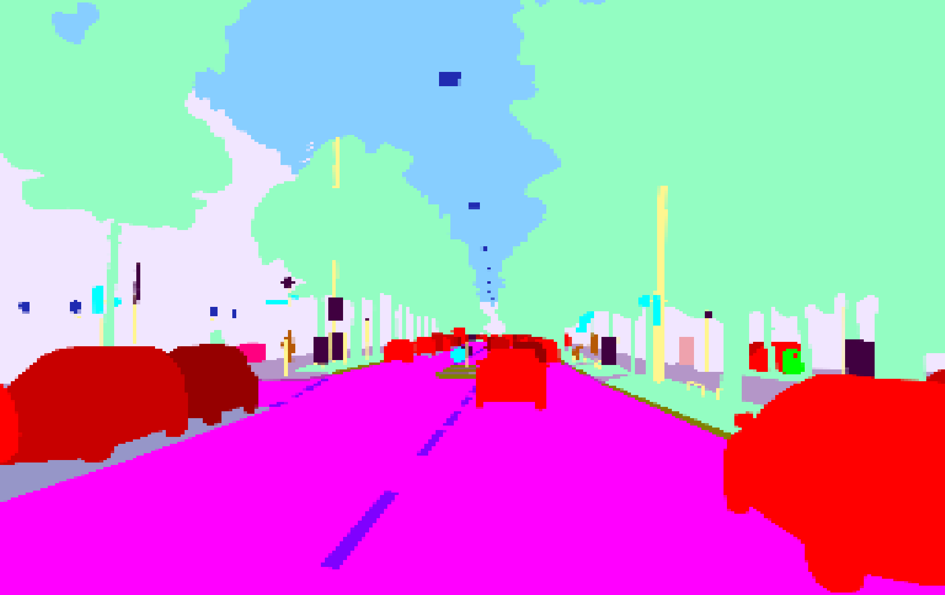
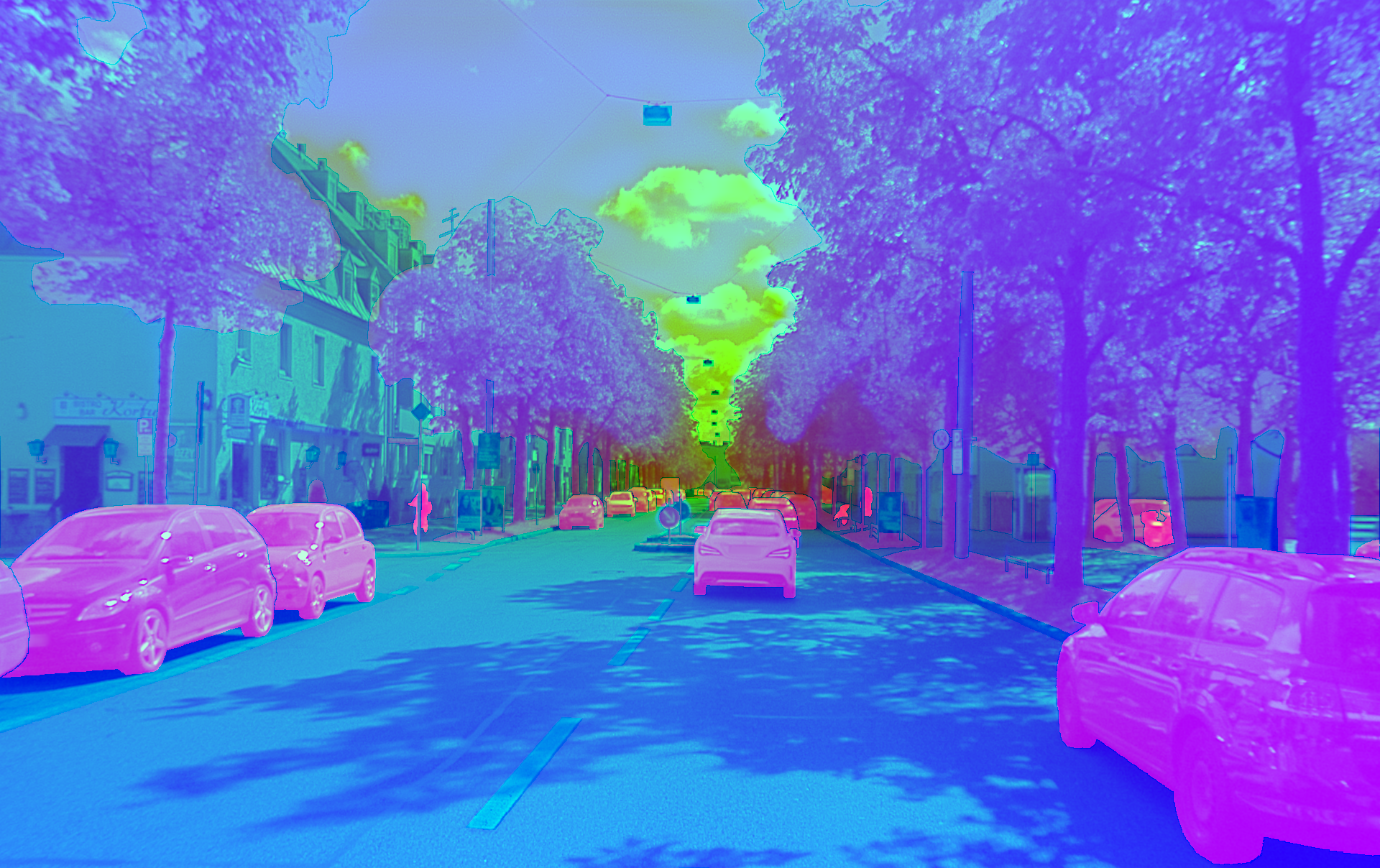
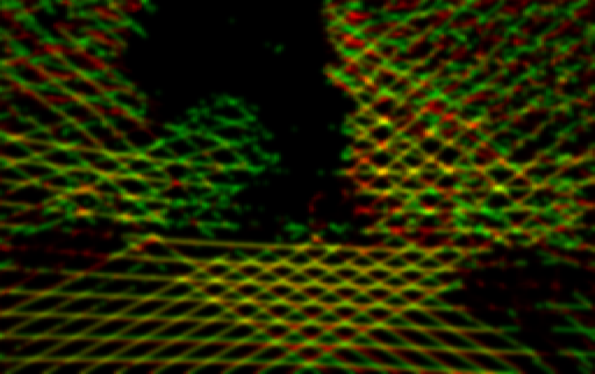
(a) Trained on Camera Images

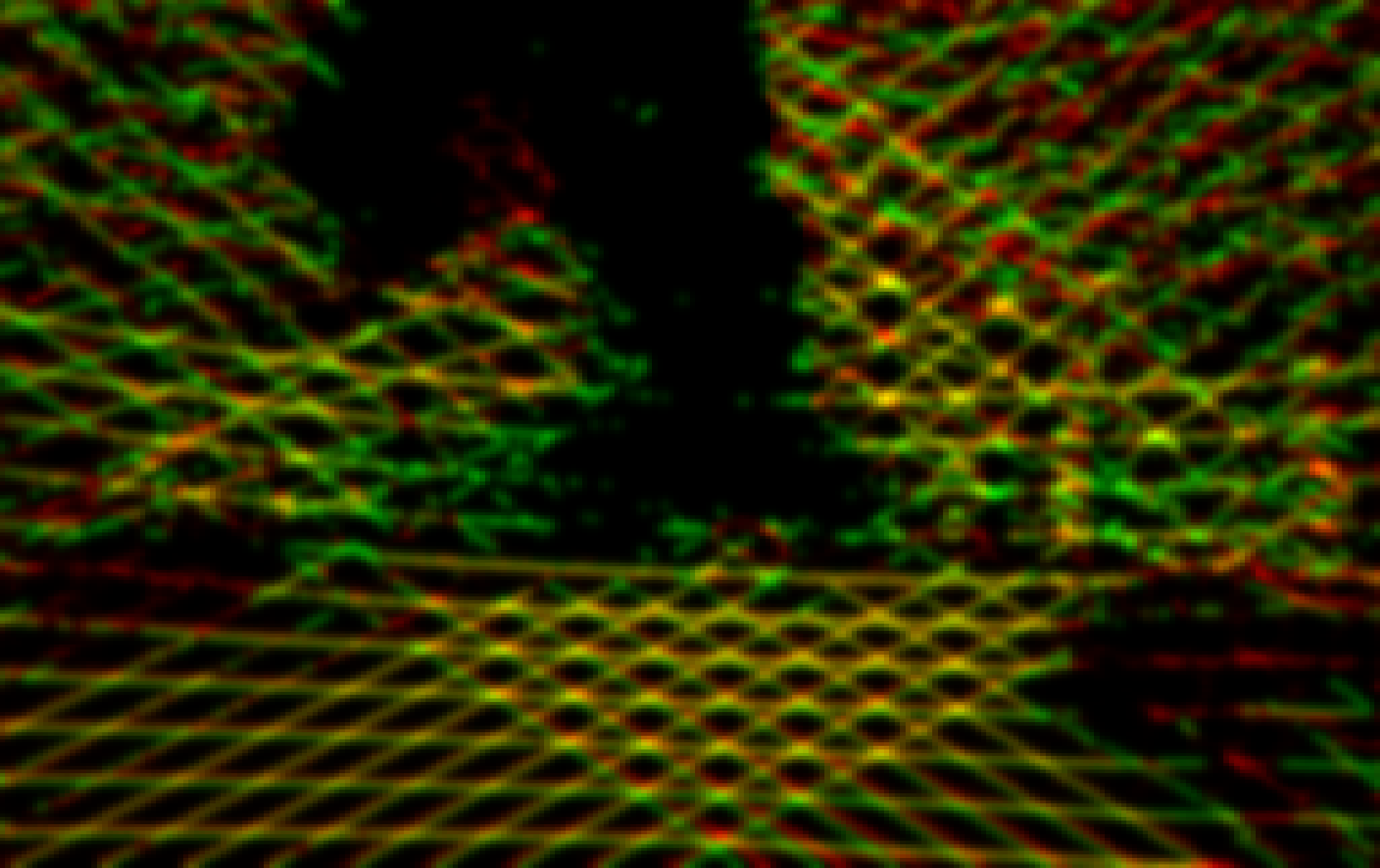
(b) Trained on Depth Maps                  

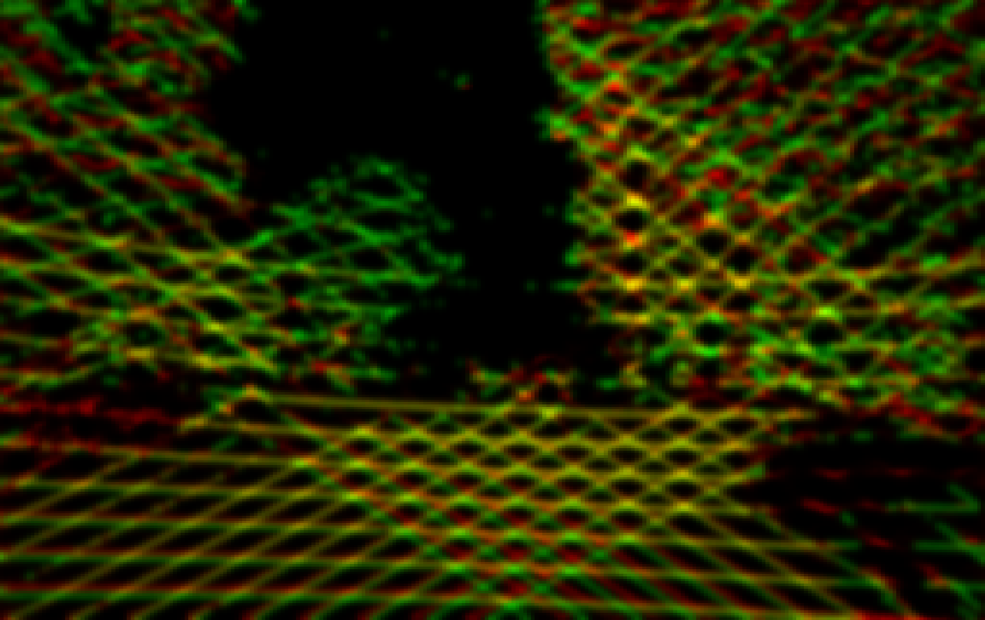
(c) Trained on Segmentation Maps

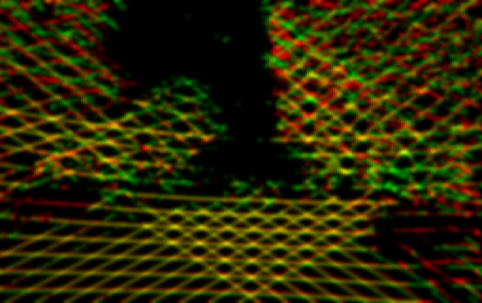
(d) Trained on Combined Images

Figure 4: Results on the A2D2 data set: lower image shows prediction (red) and ground truth (green), correctly predicted pixels are consequently yellow.

4.1 Qualitative Evaluation

Both, KITTI and A2D2 work with the same network configuration and only require different filter kernels to be applied as described in Section 3.3. Naturally, there are significant differences resulting from the different training data sets and sensor configurations; KITTI has higher LiDAR density, but a smaller upwards angle. This means that elevated objects like traffic lights or trees are often not detected correctly.

Due to the reduced number of training samples compared to A2D2, the KITTI results lack in visual quality. Concerning the sensor artifacts, we observe that the general projection pattern is acquired very well by the network. The points in the distance are also cut as limited by the sensor range but especially the variants without depth are less effective here. Individual objects, however, are harder to distinguish by eye and reflection effects are inconsistent. With a learning based approach, there is an upper limit to what is possible, given the available input. In reality, there are objects that appear very similar on camera but have very different reflection attributes.

4.2 Quantitative Evaluation

For training we have used an Nvidia RTX 3080. We use 32k training steps which can be completed in less than half an hour, so our pipeline can be trained quickly for new sensor configurations. Depending on the data set, the network has not necessarily seen every input picture once, but since consecutive frames are very similar, more training has shown no benefit in our experiments. Inference on the same GPU takes 17ms without any optimizations, which allows real-time LiDAR simulation.

To evaluate the quality of our results, we predict LiDAR images on real-world input from KITTI and A2D2 and compare these with ground truth LiDAR data. Depth images are estimated from the RGB images and as segmentation masks we use ground truth data from the data sets.

Table 1: Evaluation on KITTI, A2D2 and VKITTI: Errors on respective test set in percent.

	$L1$	$L1^{+}$	$L1^{-}$	$L2$
KITTI RGB	8.64	6.14	2.50	14.33
KITTI Depth	8.08	4.92	3.16	13.58
KITTI Sem	8.72	5.90	2.82	14.44
KITTI Com	8.63	4.96	3.67	14.36
A2D2 RGB	10.52	5.44	5.08	17.02
A2D2 Depth	10.22	5.36	4.86	16.63
A2D2 Sem	10.55	10.16	0.39	17.02
A2D2 Com	10.38	6.01	4.38	16.90
VKITTI RGB	8.33	4.28	4.05	14.06
VKITTI Depth	8.64	4.88	3.76	14.26
VKITTI Sem	8.26	3.94	4.32	13.89
VKITTI Com	8.39	4.71	3.68	13.98

We compute the $L1$ error ($L1=|A-B|$) where $A$ is the prediction and $B$ is the ground truth). Moreover, we define a positive error $L1^{+}=\max(A-B,0)$, where the network predicts points that are not present in the ground truth, and a negative error $L1^{-}=\max(B-A,0)$, where points are missing in the prediction. Additionally, we compute the $L2$ error.

The results in Tab. 1 show that the prediction results for RGB, depth, segmentation, and combined are relatively close. Prediction on KITTI data works better than for A2D2, which partly results from the larger black space in the LiDAR projections. Depth seems to work generally well, and since it is generated in any simulation anyhow, it looks like a good candidate for integration. However, one would have to examine closer, whether features important for the following task are well represented, e.g. car windows. The combined mode showed no advantage, however smarter ways to combine the three modalities might deliver better results.

Overall, the quality of images trained in a network like pix2pix cannot fully be estimated by pixel-wise errors. Small shifts in the LiDAR pattern, for example, result in large errors. Fig. 4 overlays the ground truth and the prediction, showing deviations between the different input types, most prominently in the distant parts, where a correct depth estimation becomes important.

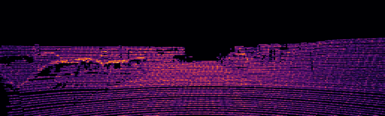
(a) Ground Truth LiDAR Image

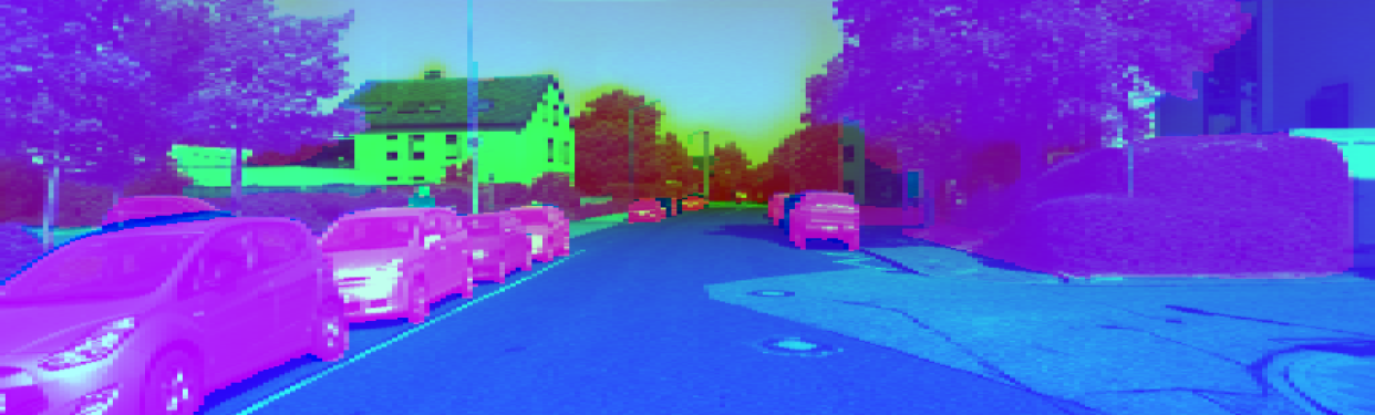
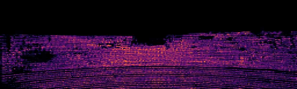
(b) KITTI Prediction from Combined Image

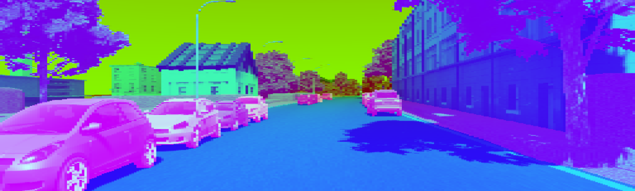
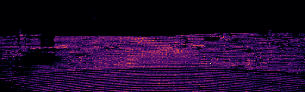
(c) VKITTI Prediction from Combined Image

Figure 5: Comparing Results on VKITTI and KITTI. The input image on top of (b) and (c) shows the combined image with RGB (grayscale), depth and segmentation in the color channels.

For an evaluation of the generalization of our method to synthetic data, we use paired data from KITTI and VKITTI. We use networks trained on real-world data and apply them to synthetic images from VKITTI. We predict LiDAR images and compare the results with the ground truth LiDAR data from KITTI as shown in Fig. 5. Results are shown in Tab. 1. Results of this comparison strongly depend on the deviation between KITTI and VKITTI data, however, our results still show good correspondence and a behavior comparable to real world data.

5 DISCUSSION

With our approach of trying to obtain typical and realistic LiDAR data, we accept a higher numerical error. The problem here is that there is no reference for a visual or numerical comparison to existing data based approaches. The quality of physics based simulation on the other hand depends not only on the implementation of the sensor system but also on the environment. Even LiDARsim already operates on the aggregated real world data geometry data, which makes a direct result based comparison unfeasible.

The consequence would be to use indirect measures, e.g. follow the sim-to-real approach and select appropriate machine learning algorithms that take point clouds as input and are trained on real data. This allows to compare the performance between using real and synthetic point cloud sources. A second option would be to augment training data for such a network with synthetic point clouds to reduce the need for real world data collection. But only a high quality virtual twin of an environment would allow a direct comparison. Especially the geometry ground truth data does not align closely enough in VKITTI (cf. Fig: 5), as the scene is here constructed from a predefined set of objects. We believe that finding ways to better measure realistic simulation will be an important task to achieve virtual testing of ADAS.

Based on the results of LiDAR simulation with pix2pix, experiments with other architectures become very interesting. However, these often make specific assumptions. So there is a need for an architecture that is also specialized for this task and can make better use of combined input data.

On the other hand, the quality of the training data is arguably even more important. There are developments that can significantly improve this: Better sensors and thus denser LiDAR scans would reduce the resolution discrepancy between camera images and LiDAR scans. Similarly, progress in 3d scene reconstruction can improve the data situation as well, but the issues with dynamic objects and movement in general currently can introduce further problems.

Given these possible developments, it is important to have a baseline for future performance comparisons, which our pipeline provides.

6 CONCLUSION

We have presented a pipeline for data based simulation of LiDAR sensor behaviour, that generalizes rather well for synthetic data inputs in simulation environments. While the general quality is not reliable enough for prediction of frame-accurate sensor artefacts, the LiDAR simulation is capable of reproducing them in general. We believe it is sufficient for many use cases, that analyse the performance of ADAS functions over many virtual road miles. With the rapid developments of LiDAR technology, better data sets will emerge naturally, while existing data sets can be enhanced with new data fusion techniques to exploit multiple consecutive frames.

REFERENCES

- Automotive, 2020 Automotive, I. (2020). CarMaker. Publisher: IPG Automotive GmbH.
- Cabon et al., 2020 Cabon, Y., Murray, N., and Humenberger, M. (2020). Virtual kitti 2.
- Dosovitskiy et al., 2017 Dosovitskiy, A., Ros, G., Codevilla, F., Lopez, A., and Koltun, V. (2017). CARLA: An Open Urban Driving Simulator. arXiv:1711.03938 [cs]. arXiv: 1711.03938.
- Gaidon et al., 2016 Gaidon, A., Wang, Q., Cabon, Y., and Vig, E. (2016). Virtual worlds as proxy for multi-object tracking analysis.
- Goodfellow et al., 2014 Goodfellow, I. J., Pouget-Abadie, J., Mirza, M., Xu, B., Warde-Farley, D., Ozair, S., Courville, A., and Bengio, Y. (2014). Generative adversarial networks.
- Isola et al., 2018 Isola, P., Zhu, J.-Y., Zhou, T., and Efros, A. A. (2018). Image-to-Image Translation with Conditional Adversarial Networks. arXiv:1611.07004 [cs]. arXiv: 1611.07004.
- Johnson et al., 2016 Johnson, J., Alahi, A., and Fei-Fei, L. (2016). Perceptual Losses for Real-Time Style Transfer and Super-Resolution. arXiv:1603.08155 [cs]. arXiv: 1603.08155.
- Kirillov et al., 2019 Kirillov, A., Wu, Y., He, K., and Girshick, R. B. (2019). Pointrend: Image segmentation as rendering. CoRR, abs/1912.08193.
- LG, 2021 LG (2021). LGSVL Simulator, https://www.lgsvlsimulator.com/.
- Liao et al., 2021 Liao, Y., Xie, J., and Geiger, A. (2021). KITTI-360: A novel dataset and benchmarks for urban scene understanding in 2d and 3d. arXiv.org, 2109.13410.
- Manivasagam et al., 2020 Manivasagam, S., Wang, S., Wong, K., Zeng, W., Sazanovich, M., Tan, S., Yang, B., Ma, W.-C., and Urtasun, R. (2020). LiDARsim: Realistic LiDAR Simulation by Leveraging the Real World. arXiv:2006.09348 [cs]. arXiv: 2006.09348.
- NVIDIA, 2021 NVIDIA (2021). Nvidia drive sim, https://developer.nvidia.com/drive/drive-sim.
- Park et al., 2019 Park, T., Liu, M.-Y., Wang, T.-C., and Zhu, J.-Y. (2019). Semantic image synthesis with spatially-adaptive normalization. In Proceedings of the IEEE Conference on Computer Vision and Pattern Recognition.
- Ranftl et al., 2021 Ranftl, R., Bochkovskiy, A., and Koltun, V. (2021). Vision transformers for dense prediction. ArXiv preprint.
- Ronneberger et al., 2015 Ronneberger, O., Fischer, P., and Brox, T. (2015). U-net: Convolutional networks for biomedical image segmentation.
- Shah et al., 2017 Shah, S., Dey, D., Lovett, C., and Kapoor, A. (2017). AirSim: High-Fidelity Visual and Physical Simulation for Autonomous Vehicles. arXiv:1705.05065 [cs]. arXiv: 1705.05065.
- Shorten and Khoshgoftaar, 2019 Shorten, C. and Khoshgoftaar, T. M. (2019). A survey on Image Data Augmentation for Deep Learning. Journal of Big Data, 6(1):60.
- Sun et al., 2020 Sun, P., Kretzschmar, H., Dotiwalla, X., Chouard, A., Patnaik, V., Tsui, P., Guo, J., Zhou, Y., Chai, Y., Caine, B., Vasudevan, V., Han, W., Ngiam, J., Zhao, H., Timofeev, A., Ettinger, S., Krivokon, M., Gao, A., Joshi, A., Zhao, S., Cheng, S., Zhang, Y., Shlens, J., Chen, Z., and Anguelov, D. (2020). Scalability in Perception for Autonomous Driving: Waymo Open Dataset. arXiv:1912.04838 [cs, stat]. arXiv: 1912.04838.
- Uhrig et al., 2017 Uhrig, J., Schneider, N., Schneider, L., Franke, U., Brox, T., and Geiger, A. (2017). Sparsity invariant cnns. In International Conference on 3D Vision (3DV).
- VTD, 2021 VTD (2021). Virtual Test Drive.
- Wang et al., 2020 Wang, L., Goldluecke, B., and Anklam, C. (2020). L2r gan: Lidar-to-radar translation. In Proceedings of the Asian Conference on Computer Vision (ACCV).
- Wang et al., 2018a Wang, T.-C., Liu, M.-Y., Zhu, J.-Y., Tao, A., Kautz, J., and Catanzaro, B. (2018a). High-resolution image synthesis and semantic manipulation with conditional gans. In Proceedings of the IEEE Conference on Computer Vision and Pattern Recognition.
- Wang et al., 2018b Wang, Y., Chao, W.-L., Garg, D., Hariharan, B., Campbell, M., and Weinberger, K. Q. (2018b). Pseudo-LiDAR from Visual Depth Estimation: Bridging the Gap in 3D Object Detection for Autonomous Driving. arXiv:1812.07179 [cs]. arXiv: 1812.07179.
- Weber et al., 2021 Weber, M., Xie, J., Collins, M., Zhu, Y., Voigtlaender, P., Adam, H., Green, B., Geiger, A., Leibe, B., Cremers, D., Osep, A., Leal-Taixe, L., and Chen, L.-C. (2021). Step: Segmenting and tracking every pixel. In Neural Information Processing Systems (NeurIPS) Track on Datasets and Benchmarks.
- Zhu et al., 2020 Zhu, J.-Y., Park, T., Isola, P., and Efros, A. A. (2020). Unpaired Image-to-Image Translation using Cycle-Consistent Adversarial Networks. arXiv:1703.10593 [cs]. arXiv: 1703.10593.