A Strengthened SDP Relaxation for Quadratic Optimization Over the Stiefel Manifold

Abstract

We study semidefinite programming (SDP) relaxations for the NP-hard problem of globally optimizing a quadratic function over the Stiefel manifold. We introduce a strengthened relaxation based on two recent ideas in the literature: (i) a tailored SDP for objectives with a block-diagonal Hessian; (ii) and the use of the Kronecker matrix product to construct SDP relaxations. Using synthetic instances on four problem classes, we show that, in general, our relaxation significantly strengthens existing relaxations, although at the expense of longer solution times.

Keywords: quadratically constrained quadratic programming, semidefinite programming, Stiefel manifold

1 Introduction

Given positive integers $n$ and $p$, the Stiefel manifold is the set of all real $n\times p$ matrices with orthonormal columns:

$$\operatorname{St}(n,p):=\{U\in\mathbb{R}^{n\times p}:U^{T}U=I_{p}\},$$

where $I_{p}$ denotes the $p\times p$ identity matrix. We study quadratic optimization over $\operatorname{St}(n,p)$:

$$\min\left\{u^{T}Hu+2\,g^{T}u:u=\operatorname{vec}(U),\ U\in\operatorname{St}(n,p)\right\},$$ (QPS)

where $u=\operatorname{vec}(U)$ is the vector formed by stacking the columns of $U$. Here, the data are the symmetric matrix $H\in\mathbb{R}^{np\times np}$ and column vector $g\in\mathbb{R}^{np}$. We recover $U$ from $u$ via the operator $U=\operatorname{mat}(u)$, which reassembles the subvectors of $u$.

(QPS) has many applications, including subspace tracking in signal processing and control, the orthogonal Procrustes problem and its generalizations, conjugate gradient for large eigenvalue problems, clustering for data mining, and electronic structures computation [5, 9, 12, 13, 14, 17, 19, 23, 24, 25].

For $p=1$, (QPS) is the well-known trust-region subproblem, which is polynomial-time solvable [20]. On the other hand, problem (QPS) is NP-hard for general $p$. In particular, [21] (page 303) discusses this computational complexity for the case $g\neq 0$ and $p=n$. Accordingly, many researchers have focused on iterative methods to obtain stationary points or local minimizers [1, 6] as well as convex relaxations of (QPS), e.g., via semidefinite programming, to obtain tight, valid lower bounds on its optimal value [2, 3, 11, 21, 22]. In this paper, we are interested in deriving strengthened SDP relaxations of (QPS).

As a quadratically constrained quadratic program, (QPS) has a standard semidefinite programming (SDP) relaxation, called the Shor relaxation, which we describe in Section 2 and denote as Shor. In a recent paper, Gilman et al. [15] studied instances of (QPS) with block-diagonal $H$, and they adapted the Shor relaxation to this block structure. In addition, they introduced a strengthening of the Shor relaxation, which proved to be extremely effective for solving block-diagonal instances. In Section 2, we further adapt their strengthening in a straightforward manner to the case of general $H$, and we refer to this relaxation as DiagSum.

Then we introduce an additional strengthening of DiagSum. We refer to this strengthening as Kron since it is based on the Kronecker-product idea introduced by Anstreicher [4]. In particular, Anstreicher showed how to derive a valid positive-semidefinite constraint for the Shor relaxation of a quadratic program, which also includes two linear matrix inequalities (LMIs), by considering the Kronecker product of the LMIs. In our case, we will use the Kronecker product of a single redundant LMI with itself. Full details are given in Section 2.3.

We test the strength of Kron relative to DiagSum and Shor on synthetic instances for four problem classes, one of which consists of block-diagonal $H$ similar to those considered in [15]. We show that Kron significantly strengthens Shor on all four problem classes. It also improves DiagSum on three of the four classes but does not show an improvement on the block-diagonal instances. One downside of Kron is that it requires significantly more time to solve than DiagSum and Shor. We report results and solution times in Section 3.

1.1 Notation and terminology

Our notation and terminology are largely standard. We use the index $i$ to range over the set $\{1,\ldots,n\}$, and the indices $j$ and $k$ each range over $\{1,\ldots,p\}$. In addition, we write

$$u_{j}:=U_{\cdot j}\quad\forall\ j=1,\ldots,p\quad\quad\Longrightarrow\quad\quad U=\begin{pmatrix}u_{1}&\cdots&u_{p}\end{pmatrix},\quad u=\begin{pmatrix}u_{1}\\ \vdots\\ u_{p}\end{pmatrix}.$$

Note that the $(i,j)$-th component of $U$ equals the $i$-th component of $u_{j}$, i.e., $U_{ij}=[u_{j}]_{i}$. For simplicity, we write $U_{ij}=u_{ji}$, and we use pairs $(j,i)$ as a two-dimensional coordinate system for accessing entries of vectors in $\mathbb{R}^{np}$ such as $u$. For example, $u_{ji}$ refers to the entry of $u$ at position $(j-1)n+i$.

2 Three SDP Relaxations

In this section, we introduce the three SDP relaxations of (QPS) mentioned in the Introduction: Shor, DiagSum, and Kron. Shor is derived directly from (QPS) using standard techniques from the semidefinite-programming literature. Then DiagSum adds a valid constraint to Shor, similar to [15], and finally we construct Kron by adding a new valid constraint to DiagSum. This new constraint is based on the Kronecker-product idea introduced in [4]. Hence, the relaxations are ordered in terms of increasing (or more precisely, non-decreasing) strength of their lower bounds on (QPS). Our conceptual contribution in this paper is the observation that the Kronecker-product idea applies in this setting, and we will show empirically in Section 3 that Kron significantly improves the strength of Shor and DiagSum in general.

2.1 The Shor relaxation

The Shor relaxation for (QPS), which we call Shor, is derived by relaxing the quadratic form

$${1\choose u}{1\choose u}^{T}=\begin{pmatrix}1\\ u_{1}\\ \vdots\\ u_{p}\end{pmatrix}\begin{pmatrix}1\\ u_{1}\\ \vdots\\ u_{p}\end{pmatrix}^{T}\in\mathbb{S}^{1+np}$$

to the positive semidefinite matrix

$$Y:=\begin{pmatrix}1&u^{T}\\ u&X\end{pmatrix}:=\begin{pmatrix}1&u_{1}^{T}&\cdots&u_{p}^{T}\\ u_{1}&X_{11}&\cdots&X_{1p}\\ \vdots&\vdots&\ddots&\vdots\\ u_{p}&X_{p1}&\cdots&X_{pp}\end{pmatrix}\in\mathbb{S}^{1+np}_{+}$$ (1)

Note that each rank-1 outer product $u_{j}u_{k}^{T}\in\mathbb{R}^{n\times n}$ is relaxed to $X_{jk}\in\mathbb{R}^{n\times n}$. We will use a 0 index to specify the first row and column of $Y$ as well as the $ji$-coordinate system described in Section 1.1 to access the remaining rows and columns of $Y$. For example,

$$Y_{00}=1,\quad\quad Y_{\cdot 0}={1\choose u},\quad\quad Y_{\cdot ji}=\begin{pmatrix}u_{ji}\\ [X_{1j}]_{\cdot i}\\ \vdots\\ [X_{pj}]_{\cdot i}\end{pmatrix}$$

In terms of $u=\operatorname{vec}(U)$, the constraints defining $U\in\operatorname{St}(n,p)$ are $u_{j}^{T}u_{j}=1$ for all $j$ and $u_{j}^{T}u_{k}=0$ for all $j\neq k$. Hence, Shor enforces $\operatorname{trace}(X_{jj})=1$ and $\operatorname{trace}(X_{jk})=0$. Moreover, the objective function $u^{T}Hu+2\,g^{T}u$ relaxes to $H\bullet X+2\,g^{T}u$, where $H\bullet X:=\operatorname{trace}(HX)$, yielding

$$\min\ \ H\bullet X+2\,g^{T}u$$

$$\operatorname{s.t.}\ \ \operatorname{trace}(X_{jj})=1\quad\forall\ j=1,\ldots,p$$ (Shor)

$$\operatorname{trace}(X_{jk})=0\quad\forall\ j\neq k$$

$$Y\succeq 0,$$

where the optimization variables $u,X,Y$ are related according to the definition (1).

2.2 The diagonal-sum relaxation

To state the relaxation DiagSum, which is based on [15], consider the implications

$$U^{T}U=I_{p}\quad\Longrightarrow\quad U^{T}U\preceq I_{p}\quad\Longleftrightarrow\quad\begin{pmatrix}I_{p}&U^{T}\\ U&I_{n}\end{pmatrix}\succeq 0\quad\Longleftrightarrow\quad UU^{T}\preceq I_{n},$$ (2)

where $I_{n}$ denotes the $n\times n$ identity matrix. The first implication follows by relaxing the Stiefel equation $U^{T}U=I_{p}$ to a matrix inequality, and the second and third implications follow by the Schur complement theorem. Then

$$\sum_{j=1}^{p}u_{j}u_{j}^{T}=UU^{T}\preceq I_{n}\quad\Longrightarrow\quad\sum_{j=1}^{p}X_{jj}\preceq I_{n},$$

and DiagSum is formed by adding this final linear matrix inequality to the Shor relaxation:

$$\min\ \ H\bullet X+2\,g^{T}u$$

$$\operatorname{s.t.}\ \ \operatorname{trace}(X_{jj})=1\quad\forall\ j=1,\ldots,p$$

$$\operatorname{trace}(X_{jk})=0\quad\forall\ j\neq k$$ (DiagSum)

$$Y\succeq 0$$

$$\sum_{j=1}^{p}X_{jj}\preceq I_{n}.$$

In fact, [15] studied instances of (QPS) for which $H$ is a block-diagonal matrix of the form $H:=\text{Diag}\left(H_{11},\ldots,H_{pp}\right)$ with each $H_{jj}\in\mathbb{S}^{n}$. In this case, the objective function simplifies to $\sum_{j=1}^{p}H_{jj}\bullet X_{jj}+2\,g^{T}u$. The precise form of the relaxation considered in [15] then dropped the off-diagonal $X_{jk}$, considered the weaker semidefinite conditions

$$\begin{pmatrix}1&u_{j}^{T}\\ u_{j}&X_{jj}\end{pmatrix}\succeq 0\quad\forall\ j=1,\ldots,p$$

corresponding to certain principal submatrices of $Y\succeq 0$, and enforced $\sum_{j=1}^{p}X_{jj}\preceq I_{n}$.

2.3 The Kronecker relaxation

To derive Kron, we observe that the Kronecker-product idea developed in [4] can be applied in this setting. Specifically, using (2) and the fact that the Kronecker product of positive semidefinite matrices is positive semidefinite, we see that

$$\begin{pmatrix}I_{p}&U^{T}\\ U&I_{n}\end{pmatrix}\succeq 0\quad\Longrightarrow\quad\begin{pmatrix}I_{p}&U^{T}\\ U&I_{n}\end{pmatrix}\otimes\begin{pmatrix}I_{p}&U^{T}\\ U&I_{n}\end{pmatrix}\succeq 0.$$ (3)

The resultant linear matrix inequality depends quadratically on $U$, and hence it can be linearized in the space of the lifted variable $Y$. Note that the size of the Kronecker-product matrix is $(n+p)^{2}\times(n+p)^{2}$.

To determine the precise form of the linearization, define the constant matrices

$$K_{ji}=e_{p+i}e_{j}^{T}+e_{j}e_{p+i}^{T}\in\mathbb{S}^{p+n}\quad\quad\forall\ \ (j,i)\in\{1,\ldots,p\}\times\{1,\ldots,n\}.$$

We then have the expression

$$\begin{pmatrix}I_{p}&U^{T}\\ U&I_{n}\end{pmatrix} =I_{p+n}+\sum_{i=1}^{n}\sum_{j=1}^{p}U_{ij}(e_{p+i}e_{j}^{T}+e_{j}e_{p+i}^{T})$$

$$=I_{p+n}+\sum_{j=1}^{p}\sum_{i=1}^{n}u_{ji}K_{ji}.$$

Hence,

$$\begin{pmatrix}I_{p}&U^{T}\\ U&I_{n}\end{pmatrix} \otimes\begin{pmatrix}I_{p}&U^{T}\\ U&I_{n}\end{pmatrix}=I_{p+n}\otimes I_{p+n}+$$

$$\sum_{j=1}^{p}\sum_{i=1}^{n}u_{ji}(I_{p+n}\otimes K_{ji}+K_{ji}\otimes I_{p+n})+\sum_{j=1}^{p}\sum_{i=1}^{n}\sum_{k=1}^{p}\sum_{l=1}^{n}u_{ji}u_{kl}K_{ji}\otimes K_{kl},$$

and so the quadratic linear matrix inequality introduced above linearizes to $M(u,X)\succeq 0$, where

$$M(u,X):=I_{(p+n)^{2}} +\sum_{j=1}^{p}\sum_{i=1}^{n}u_{ji}(I_{p+n}\otimes K_{ji}+K_{ji}\otimes I_{p+n})+$$

$$\sum_{j=1}^{p}\sum_{i=1}^{n}\sum_{k=1}^{p}\sum_{l=1}^{n}[X_{jk}]_{il}K_{ji}\otimes K_{kl}.$$

Adding $M(u,X)\succeq 0$ to DiagSum, we obtain the Kron relaxation

$$\min\ \ H\bullet X+2\,g^{T}u$$

$$\operatorname{s.t.}\ \ \operatorname{trace}(X_{jj})=1\quad\forall\ j=1,\ldots,p$$

$$\operatorname{trace}(X_{jk})=0\quad\forall\ j\neq k$$ (Kron)

$$Y\succeq 0$$

$$\sum_{j=1}^{p}X_{jj}\preceq I_{n}$$

$$M(u,X)\succeq 0.$$

2.3.1 Two variations

Before taking the Kronecker product in (3), we could also symmetrically permute one of the two matrices to

$$\begin{pmatrix}I_{n}&U\\ U^{T}&I_{p}\end{pmatrix}\succeq 0$$

and consider the product

$$\begin{pmatrix}I_{n}&U\\ U^{T}&I_{p}\end{pmatrix}\otimes\begin{pmatrix}I_{p}&U^{T}\\ U&I_{n}\end{pmatrix}\succeq 0.$$

However, after linearization, it is not difficult to see that this would simply lead to a permutation of $M(u,X)\succeq 0$ and hence would not generate a new valid constraint. In fact, any symmetric permutation will lead to the same constraint $M(u,X)\succeq 0$.

Instead of considering the Kronecker product, we could use the fact that the Hadamard product (indicated by the “$\circ$” symbol) of positive semidefinite matrices is positive semidefinite to relax the $(n+p)\times(n+p)$ condition

$$\begin{pmatrix}I_{p}&U^{T}\\ U&I_{n}\end{pmatrix}\circ\begin{pmatrix}I_{p}&U^{T}\\ U&I_{n}\end{pmatrix}\succeq 0$$

to

$$\begin{pmatrix}I_{p}&\operatorname{mat}(\operatorname{diag}(X))^{T}\\ \operatorname{mat}(\operatorname{diag}(X))&I_{n}\end{pmatrix}\succeq 0.$$ (4)

The paper [18] considered such an approach in a more general setting. It is clear that this positive semidefinite matrix is a small principal submatrix of $M(u,X)\succeq 0$, and so (4) could be added to DiagSum to form a fourth relaxation, whose strength is in between DiagSum and Kron and could be solved more quickly than Kron. Through extensive numerical experiments, however, we could find no instances for which (4) strengthens DiagSum. Said differently, it appears that DiagSum implies (4), although we have so far not been able to prove this. Due to this experience, we will not consider the Hadamard product further in this paper.

2.4 Dual bounds and primal values

For each of the three SDP relaxations developed in the preceding subsections, its optimal value $d$ is a lower bound on the optimal value $v$ of (QPS), i.e., $d\leq v$. We can also use any feasible solution $(u,X)$ of the SDP to generate a feasible value (or primal value) $p$ for (QPS) such that $d\leq v\leq p$. This provides an absolute duality gap $p-d$ on the optimal value $v$, or a relative gap $(p-d)/\max\{1,|\tfrac{1}{2}(p+d)|\}$.

Indeed, given feasible $(u,X)$ and $Y$ related by (1), if $\text{rank}(Y)$ happens to equal 1, then by construction $U:=\operatorname{mat}(u)$ is an element of $\operatorname{St}(n,p)$, and then $p:=u^{T}Hu+2\,g^{T}u$ is the desired primal value. On the other hand, if $\text{rank}(Y)>1$, we can still calculate a primal value as follows:

• let $U_{0}\Sigma_{0}V_{0}^{T}$ be the thin singular value decomposition of $U$ and define $\tilde{U}:=U_{0}V_{0}^{T}\in\operatorname{St}(n,p)$;

• then set $\tilde{u}:=\operatorname{vec}(\tilde{U})$ and $p:=\tilde{u}^{T}H\tilde{u}+2\,g^{T}\tilde{u}$.

In the numerical experiments of Section 3, we calculate $p$ from the optimal solution $(u,X)$ of the SDP. In addition, we will use the solver Manopt [7], which is a toolbox for local optimization over manifolds, to improve heuristically the value $p$ starting from the matrix $\tilde{U}$. Note that Manopt contains built-in data structures to handle the Stiefel manifold constraint. In particular, we run Manopt’s trustregions algorithm over the Stiefel manifold with its default settings. We need only supply function, gradient, and Hessian evaluations for our objective function, which are straightforward given that the function is quadratic.

3 Numerical Experiments

In this section, we evaluate the quality of the dual bounds and primal values provided by Kron in comparison with DiagSum and Shor. We also investigate the time required to solve the various SDP relaxations. We test various combinations of $(n,p)$ ranging from $(6,2)$ to $(12,11)$.

In preliminary tests, we also evaluated the global solver Gurobi version 9.5.1, which solves (QPS) by calculating a sequence of primal values and dual bounds with gaps converging to zero. With $(n,p)=(6,3)$, for example, the gaps calculated by Gurobi after 15 minutes were significantly worse than those calculated by Shor, DiagSum, and Kron each within 1 second. Moreover, Gurobi’s time and gap performance for larger values of $(n,p)$ was even worse relative to the three SDP relaxations. Hence, in what follows, we do not include explicit comparisons with Gurobi.

We first describe our problem instances and then specify our testing algorithm and measurements. Finally, we summarize our results.

3.1 Problem instances

In this subsection, we consider positive integers $n\geq p$ to be fixed. We consider four problem classes:

1. Our first class of instances is based on random $H\in\mathbb{S}^{np}$ and $g\in\mathbb{R}^{np}$ such that every entry in $H$ and $g$ is i.i.d. ${\cal N}(0,1)$. We call these the random instances.

2. Our second class of instances is the block-diagonal instances in which $H$ is a block-diagonal matrix of the form $H:=\text{Diag}\left(H_{11},\ldots,H_{pp}\right)$ with each $H_{jj}\in\mathbb{S}^{n}$. We also take $g=0$ so that $H\bullet X+2\,g^{T}u=\sum_{j=1}^{p}H_{jj}\bullet X_{jj}$. As discussed in Section 2.2, this class was the basis of the numerical experiments in [15] for a subclass of matrices $\{H_{jj}\}$ satisfying certain structural properties. For example, their matrices $H_{jj}$ were negative semidefinite. The authors found that DiagSum was typically very strong for these instances, but some instances still showed a positive gap. In our case, we randomly generate all entries of $\{H_{jj}\}$ by drawing each entry i.i.d. ${\cal N}(0,1)$.

3. Our third class is the Procrustes instances, which are random instances of the orthogonal Procrustes problem [16]. Given an additional positive integer $m$ and matrices $A\in\mathbb{R}^{m\times n}$ and $B\in\mathbb{R}^{m\times p}$, the problem is to find an orthogonal mapping of the columns of $A$ into $\mathbb{R}^{m\times p}$, which minimizes the Frobenius distance to $B$, i.e.,

   $$\min_{U\in\operatorname{St}(n,p)}\lVert AU-B\rVert_{F}^{2},$$

   where the Frobenius norm is defined by $\|M\|_{F}:=\sqrt{M\bullet M}$. This is an instance of (QPS) with

   $$H:=I_{p}\otimes(A^{T}A),\quad g:=\operatorname{vec}(-A^{T}B).$$

   Based on $n$ and $p$, to generate a Procrustes instance, we choose $m$ to be uniformly distributed between $\lceil n/2\rceil$ and $2n$, inclusive, and then we randomly generate $A$ and $B$ with entries i.i.d. ${\cal N}(0,1)$. We remark that there exist several special cases, which are known to have closed-form solutions; see [14, 8]. Three of these cases are: $A=I_{n}$ with $m=n$; $n=p$; and $p=1$.

4. Our fourth and final class is the Penrose instances, which are random instances of the Penrose regression problem, which is itself a generalization of the orthogonal Procrustes problem; see [10, 14, 5, 19]. Given two additional positive integers $m$ and $q$, and matrices $A\in\mathbb{R}^{m\times n}$, $B\in\mathbb{R}^{m\times q}$ and $C\in\mathbb{R}^{p\times q}$, the problem is

   $$\min_{U\in\operatorname{St}(n,p)}\lVert AUC-B\rVert_{F}^{2},$$

   which is an instance of (QPS) with

   $$H:=(CC^{T})\otimes(A^{T}A),\quad g:=vec(-A^{T}BC^{T}).$$

   Based on $n$ and $p$, we choose both $m$ and $q$ to be uniformly and independently distributed between $\lceil n/2\rceil$ and $2n$, inclusive, and then we randomly generate $A$, $B$, and $C$ with entries i.i.d. ${\cal N}(0,1)$. Note that, by setting $C=I_{p}$ with $q=p$, we recover the Procrustes problem as a special case.

3.2 Testing algorithm, measurements, and experiments

Given a single instance of (QPS), Algorithm 1 specifies our testing procedure on that instance. In words, we solve Shor, DiagSum, and Kron on the instance and save the corresponding relative gaps and solution times.

Algorithm 1 Approximate a Single Instance of (QPS)

1:An instance of (QPS), i.e., positive integers $n\geq p$ and data $H\in\mathbb{S}^{np}$ and $g\in\mathbb{R}^{np}$.

2:for $\text{{\sc rlx}}\in\{\text{\sc Shor},\text{\sc DiagSum},\text{\sc Kron}\}$ do

3:     Solve rlx to obtain an optimal solution $(u^{*},X^{*})$.

4:     Save the total time $t_{\text{{\sc rlx}}}$ (in seconds) for optimizing rlx.

5:     Set $d_{\text{{\sc rlx}}}=H\bullet X^{*}+2\,g^{T}u^{*}$.

6:     Calculate $p_{\text{{\sc rlx}}}$ based on $(u^{*},X^{*})$ as described in Section 2.4.

7:     Calculate the relative gap $\gamma_{\text{{\sc rlx}}}:=(p_{\text{{\sc rlx}}}-d_{\text{{\sc rlx}}})/\max\{1,|\tfrac{1}{2}(p_{\text{{\sc rlx}}}+d_{\text{{\sc rlx}}})|\}$.

8:end for

9:Relative gaps $\gamma_{\text{\sc Shor}},\gamma_{\text{\sc DiagSum}},\gamma_{\text{\sc Kron}}$ and times $t_{\text{\sc Shor}},t_{\text{\sc DiagSum}},t_{\text{\sc Kron}}$.

Based on the output of Algorithm 1, we say that a given relaxation rlx solves the instance if the relative gap $\gamma_{\text{\sc rlx}}$ is less than $10^{-4}$.

For each of the three values $n\in\{6,9,12\}$, we tested the three values $p\in\{2,\lceil n/2\rceil,n-1\}$ for a total of nine pairs $(n,p)$ ranging from $(6,2)$ to $(12,11)$. For a fixed pair $(n,p$), we ran Algorithm 1 on 1,000 instances of each of the four problem classes described in Section 3.1.

All experiments were coded in MATLAB (version 9.11.0.1873467, R2021b Update 3), and all SDP relaxations were solved with Mosek (version 9.3.10). Manopt version 7.0 was employed for the local optimization subroutine described in Section 2.4. The computing environment was a single Xeon E5-2680v4 core running at 2.4 GHz with 8 GB of memory under the CentOS Linux operating system.

For Shor and DiagSum, we call Mosek directly, whereas we construct Kron using the modeling interface YALMIP (version 31-March-2021), which then calls Mosek. YALMIP is used for coding simplicity, since the Kronecker constraint was relatively challenging to implement directly in Mosek. Furthermore, we verified in two ways that the model passed to YALMIP from Mosek was an efficient representation of Kron. First, we used YALMIP’s dualize command to test the dual formulation; it required significantly more time to solve. Second, we verified that the problem size reported by Mosek matched what one would expect from a direct implementation of Kron.

3.3 Results

We first summarize the solution times in Table 1, which shows the average times (in seconds) for the three SDP relaxations over all instances, grouped by the nine $(n,p)$ pairs. It is clear that Kron requires significantly more time than both Shor and DiagSum as $n$ and $p$ increase. DiagSum also requires more time than Shor, but its growth with $n$ and $p$ is much more modest than Kron’s.

$n$	$p$	Shor	DiagSum	Kron
6	2	0.011	0.031	0.626
6	3	0.016	0.040	1.027
6	5	0.037	0.108	3.008
9	2	0.015	0.066	2.284
9	5	0.198	0.359	11.645
9	8	0.618	0.864	47.000
12	2	0.025	0.142	6.297
12	6	0.584	0.875	54.389
12	11	0.707	0.813	250.233

Table 1: Average solution times (in seconds) for the three SDP relaxations over all instances, grouped by the nine $(n,p)$ pairs

Next, we examine the relative gaps in Figures 1–4. Each figure corresponds to one problem class and shows the histograms of the relative gaps (depicted as line charts, or “frequency polygons,” for visibility) for Shor, DiagSum and Kron over all instances of that problem class—9,000 instances in total since there are 1,000 instances for each of the nine $(n,p)$ pairs. As discussed in Section 2.4, an instance is solved by a relaxation if the relative gap is less than $10^{-4}$. Such instances are grouped in the Solved category in the figure.

For the random instances in Figure 1, it is clear that Kron is the strongest relaxation with more instances solved and generally lower relative gaps. On the other hand, the remaining figures show different patterns. For the block-diagonal instances in Figure 2, Kron showed little to no improvement over DiagSum, whereas both relaxations significantly strengthened Shor. For the Procrustes and Penrose instances in Figures 3–4, the performance of Kron is dramatically better than both Shor and DiagSum, where Kron solved nearly all instances. (Although it is difficult to see in the figures, there were a few instances not solved by Kron.)

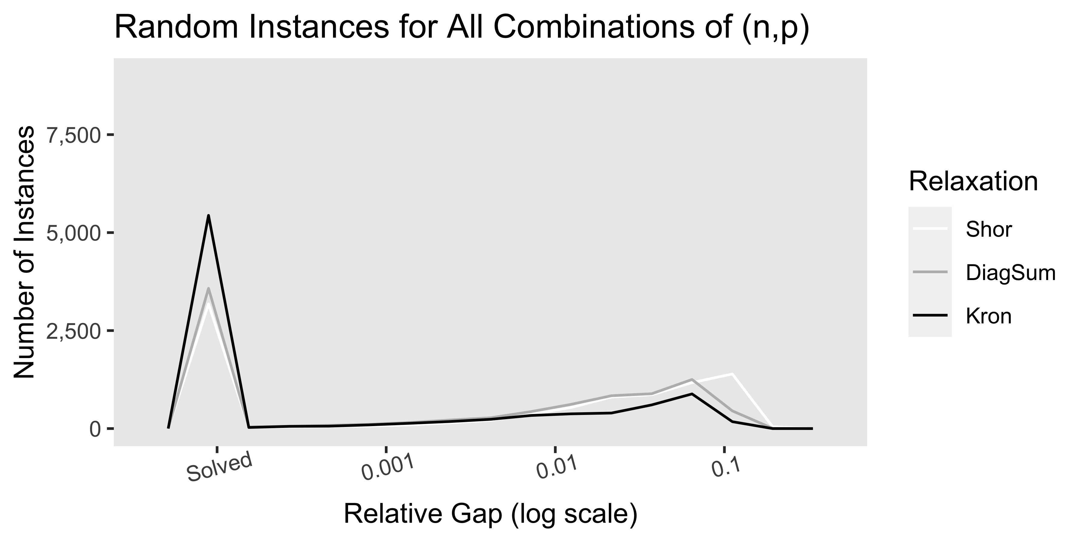
Figure 1: Histograms (depicted as line charts) of the relative gaps for the three SDP relaxations on 9,000 random instances

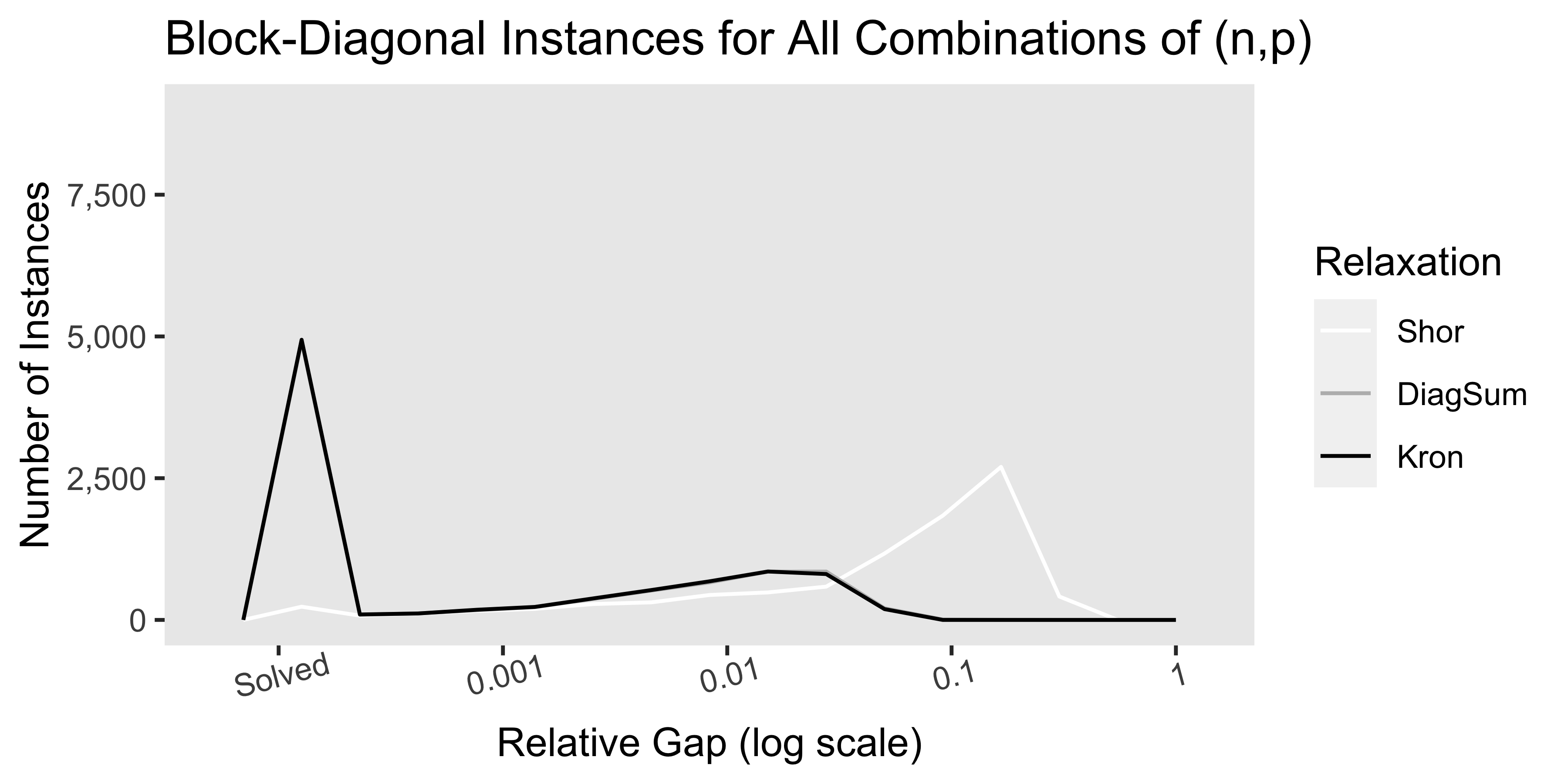
Figure 2: Histograms (depicted as line charts) of the relative gaps for the three SDP relaxations on 9,000 block-diagonal instances

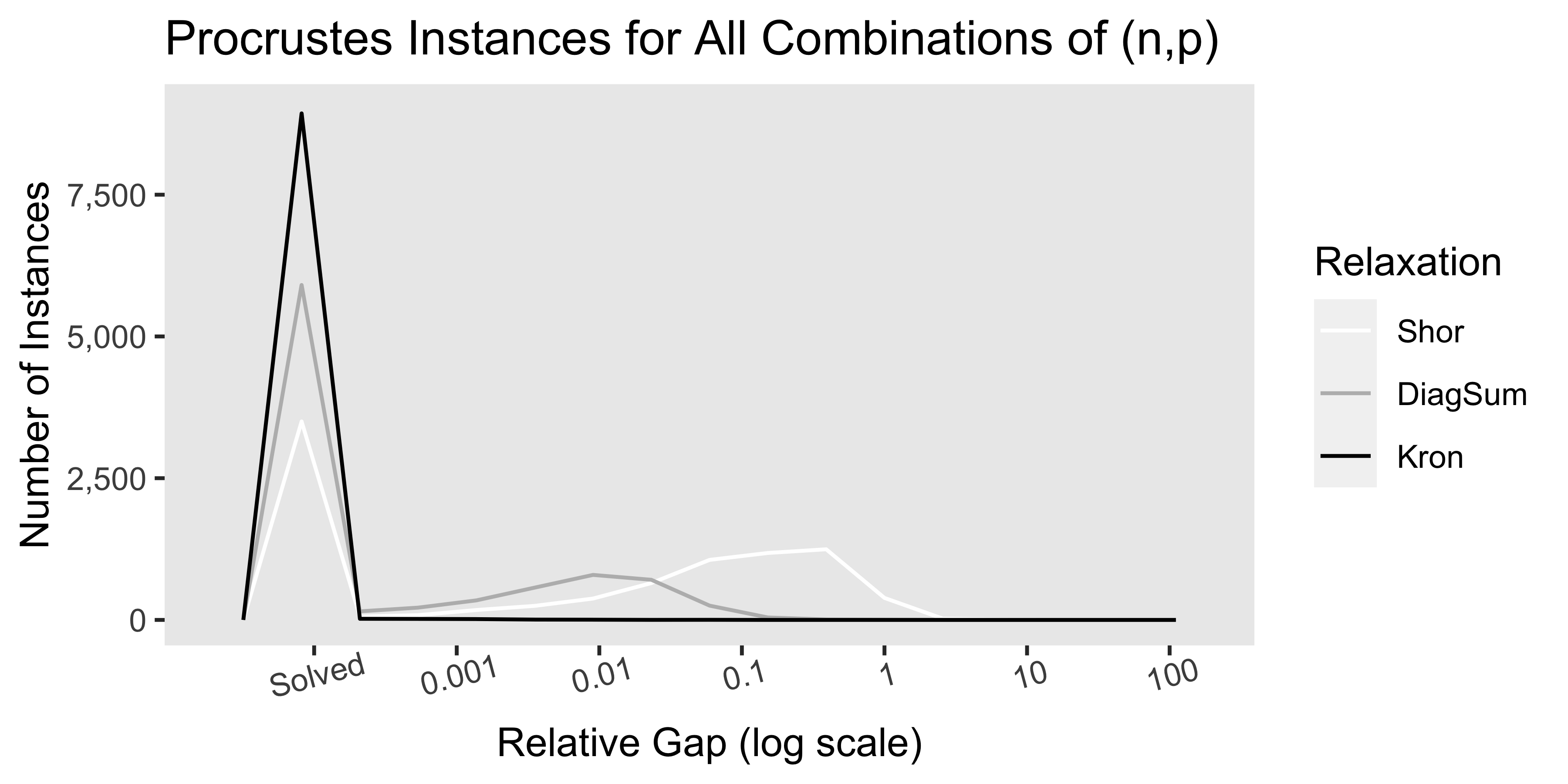
Figure 3: Histograms (depicted as line charts) of the relative gaps for the three SDP relaxations on 9,000 Procrustes instances

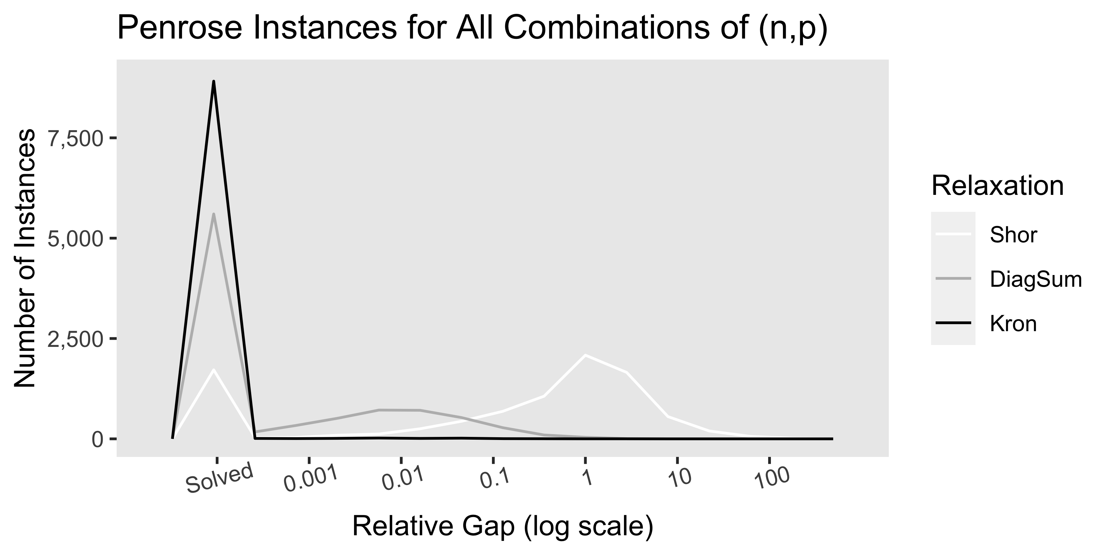
Figure 4: Histograms (depicted as line charts) of the relative gaps for the three SDP relaxations on 9,000 Penrose instances

4 Conclusions

We have shown how the Kronecker-product idea can be applied to improve SDP relaxations of (QPS), although the key constraint—the linear matrix inequality $M(u,X)\succeq 0$—adds to the complexity and time required to solve the relaxation. An area of future research would be to incorporate the strength of the Kronecker constraint without incurring the full computational cost, e.g., by a clever cutting plane method or by enforcing positive semidefiniteness on critical principal submatrices of $M(u,X)$.

Given the small relative gaps in Figure 3–4 on the Procrustes and Penrose instances, it is worthwhile to investigate whether one can prove a guaranteed quality of Kron on these problem classes. Numerically, we found that Kron did not solve all instances exactly, but given that numerical computation is necessarily inexact and relies on, for example, the accuracy of the underlying SDP solver, it would be interesting to either exhibit analytically an instance for which Kron is inexact or to prove that Kron is tight for the Procrustes or Penrose classes.

Another avenue for improvement would be to extend the theoretical results of Gilman et al [15], from which we adapted the DiagSum relaxation. Indeed, their work provides a global optimality certificate for a block-diagonal instance of (QPS) by solving a dimension-reduced SDP feasibility problem, which is closely related to their SDP relaxation. Perhaps these results could be brought to bear on our problem for general $H$.

References

- [1] P.-A. Absil, R. Mahony, and R. Sepulchre. Optimization algorithms on matrix manifolds. Princeton University Press, Princeton, NJ, 2008. With a foreword by Paul Van Dooren.
- [2] K. Anstreicher, X. Chen, H. Wolkowicz, and Y.-X. Yuan. Strong duality for a trust-region type relaxation of the quadratic assignment problem. Linear Algebra Appl., 301(1-3):121–136, 1999.
- [3] K. Anstreicher and H. Wolkowicz. On lagrangian relaxation of quadratic matrix constraints. SIAM Journal on Matrix Analysis and Applications, 22(1):41–55, 2000.
- [4] K. M. Anstreicher. Kronecker product constraints with an application to the two-trust-region subproblem. SIAM Journal on Optimization, 27(1):368–378, 2017.
- [5] P. Birtea, I. Caşu, and D. Comănescu. Second order optimality on orthogonal stiefel manifolds. Bulletin des Sciences Mathématiques, 161:102868, 2020.
- [6] N. Boumal. An introduction to optimization on smooth manifolds. To appear with Cambridge University Press, Apr 2022.
- [7] N. Boumal, B. Mishra, P.-A. Absil, and R. Sepulchre. Manopt, a Matlab toolbox for optimization on manifolds. Journal of Machine Learning Research, 15(42):1455–1459, 2014.
- [8] A. Breloy, S. Kumar, Y. Sun, and D. P. Palomar. Majorization-minimization on the stiefel manifold with application to robust sparse pca. IEEE Transactions on Signal Processing, 69:1507–1520, 2021.
- [9] S. Chrétien and B. Guedj. Revisiting clustering as matrix factorisation on the stiefel manifold. In International Conference on Machine Learning, Optimization, and Data Science, pages 1–12. Springer, 2020.
- [10] M. T. Chu and T. T. Nickolay. The orthogonally constrained regression revisited. 1997.
- [11] M. Dodig, M. Stošić, and J. Xavier. On minimizing a quadratic function on stiefel manifold. Linear Algebra and its Applications, 475:251–264, 2015.
- [12] A. Edelman, T. A. Arias, and S. T. Smith. The geometry of algorithms with orthogonality constraints. SIAM journal on Matrix Analysis and Applications, 20(2):303–353, 1998.
- [13] L. Eldén. Algorithms for the regularization of ill-conditioned least squares problems. BIT Numerical Mathematics, 17(2):134–145, 1977.
- [14] L. Eldén and H. Park. A procrustes problem on the stiefel manifold. Numerische Mathematik, 82(4):599–619, 1999.
- [15] K. Gilman, S. Burer, and L. Balzano. A semidefinite relaxation for sums of heterogeneous quadratics on the stiefel manifold, 2022.
- [16] J. C. Gower and G. B. Dijksterhuis. Procrustes problems, volume 30. OUP Oxford, 2004.
- [17] J. Hu, X. Liu, Z.-W. Wen, and Y.-X. Yuan. A brief introduction to manifold optimization. Journal of the Operations Research Society of China, 8(2):199–248, 2020.
- [18] R. Jiang and D. Li. Second order cone constrained convex relaxations for nonconvex quadratically constrained quadratic programming. J. Global Optim., 75(2):461–494, 2019.
- [19] J. Kim, M. Kang, D. Kim, S.-Y. Ha, and I. Yang. A stochastic consensus method for nonconvex optimization on the stiefel manifold. In 2020 59th IEEE Conference on Decision and Control (CDC), pages 1050–1057. IEEE, 2020.
- [20] J. J. Moré and D. C. Sorensen. Computing a trust region step. SIAM J. Sci. Statist. Comput., 4(3):553–572, 1983.
- [21] A. Nemirovski. Sums of random symmetric matrices and quadratic optimization under orthogonality constraints. Math. Program., 109(2-3, Ser. B):283–317, 2007.
- [22] M. L. Overton and R. S. Womersley. On the sum of the largest eigenvalues of a symmetric matrix. SIAM Journal on Matrix Analysis and Applications, 13(1):41–45, 1992.
- [23] S. T. Smith. Geometric optimization methods for adaptive filtering. PhD thesis, Harvard University, Cambridge, MA, May 1993.
- [24] Z. Wen and W. Yin. A feasible method for optimization with orthogonality constraints. Mathematical Programming, 142(1):397–434, 2013.
- [25] X. Zhang, J. Zhu, Z. Wen, and A. Zhou. Gradient type optimization methods for electronic structure calculations. SIAM Journal on Scientific Computing, 36(3):C265–C289, 2014.