Accelerating the Sinkhorn algorithm for sparse multi-marginal optimal transport by fast Fourier transforms

Abstract

We consider the numerical solution of the discrete multi-marginal optimal transport (MOT) by means of the Sinkhorn algorithm. In general, the Sinkhorn algorithm suffers from the curse of dimensionality with respect to the number of marginals. If the MOT cost function decouples according to a tree or circle, its complexity is linear in the number of marginal measures. In this case, we speed up the convolution with the radial kernel required in the Sinkhorn algorithm by non-uniform fast Fourier methods. Each step of the proposed accelerated Sinkhorn algorithm with a tree-structured cost function has a complexity of $\mathcal{O}(KN)$ instead of the classical $\mathcal{O}(KN^{2})$ for straightforward matrix–vector operations, where $K$ is the number of marginals and each marginal measure is supported on at most $N$ points. In case of a circle-structured cost function, the complexity improves from $\mathcal{O}(KN^{3})$ to $\mathcal{O}(KN^{2})$. This is confirmed by numerical experiments.

1 Introduction

The optimal transport (OT) problem is an optimization problem that deals with the search for an optimal map (plan) that moves masses between two or more measures at low cost [44, 55]. OT appears in a wide range of applications such as image and signal processing [7, 14, 52, 54, 56], economics [18, 27], finance [21, 22], and physics [26, 29]. The OT problem was first introduced in 1781 by Monge. His objective was to find a map between two probability measures $\mu^{1},\mu^{2}$ on $\mathbb{R}^{d}$ that transports $\mu^{1}$ to $\mu^{2}$ with minimal cost, where the cost function describes the cost of transporting mass between two points in $\mathbb{R}^{d}$. However, such maps do not always exist, so that Kantorovich [31] relaxed the problem in 1942 by looking for a transport plan with two prescribed marginals $\mu^{1}$ and $\mu^{2}$ that minimizes a certain cost functional.

Several authors have generalized the formulation to multi-marginal optimal transport (MOT) [36, 42, 43], where more than two marginal measures are given. For given probability measures $\mu^{k}$ on $\Omega^{k}\subset\mathbb{R}^{d}$, $k=1,\dots,K$, an optimal transport plan $\pi$ is defined as a solution of the MOT problem

$$\min_{\pi\in\Pi(\mu^{1},\ldots,\mu^{k})}\int_{\Omega^{1}\times\dots\times\Omega^{K}}c(x^{1},\ldots,x^{K})\,\mathrm{d}\pi(x^{1},\ldots,x^{K})$$ (1)

where $\Pi(\mu^{1},\cdots,\mu^{K})$ is the convex set of all joint probability measures $\pi$ whose marginals are $\mu^{k}$, and $c\colon\Omega^{1}\times\dots\times\Omega^{K}\to\mathbb{R}$ is the cost function.

Since the numerical computation of a transport plan is difficult in general, a regularization term such as the entropy [10, 29], Kullback-Leibler divergence [41], general $f$-divergence [53] or $L^{2}$-regularization [13, 37] can be added to make the problem strictly convex. Different approaches such as the Sinkhorn algorithm [29, 44], stochastic gradient descent [28], the Gauss-Seidel method [37], or the proximal splitting [5] have been used to iteratively determine a minimizing sequence of the MOT problem.

However, the problem suffers from the curse of dimensionality as the complexity grows exponentially with the number $K$ of marginal measures. One way to circumvent this lies in incorporating additional sparsity assumptions into the model. Polynomial-time algorithms to solve certain sparse MOT problems have been studied in [4, 9, 29]. We will assume that the cost function decouples according to a graph, where the nodes correspond to the marginals and the cost function is the sum of functions that depend only on two variables which correspond to two marginals connected by an edge of the graph. For example, the circle-structured Euclidean cost function reads as

$$c(x^{1},\dots,x^{K})=\left\lVert x^{1}-x^{2}\right\rVert_{2}^{2}+\dots+\left\lVert x^{K-1}-x^{K}\right\rVert_{2}^{2}+\left\lVert x^{K}-x^{1}\right\rVert_{2}^{2},\quad x^{1},\dots,x^{K}\in\mathbb{R}^{d}.$$

MOT problems with graph-structured cost functions with constant treewidth can be solved with the Sinkhorn algorithm in polynomial time [34]. In [4], polynomial-time algortihms were presented for the MOT problem and its regularized counterpart for the cases of a graph structure, a set-optimization structure, as well as a low-rank and sparsely structured cost function. Another sparsity assumption lies on the transport plan to be thinly spread, which is e.g. the case for the $L^{2}$-regularized problem [13, 37].

Our contributions.

In the present paper, we study the discrete, entropy-regularized MOT problem with a tree-structured [7, 29] or a circle-structured cost function, where all measures are supported on a finite number of points (atoms) in $\mathbb{R}^{d}$. Then the computational time of the Sinkhorn algorithm [2, 19, 33], which iteratively determines a sequence converging to the solution, depends linearly on the number $K$ of input measures. If the numbers of atoms is large, however, the Sinkhorn algorithm still requires considerable computational time and memory, which mainly comes from computing a discrete convolution, i.e. a matrix–vector product with a kernel matrix.

This is significantly improved by Fourier-based fast summation methods [46, 47]. The key idea is the approximation of the kernel function by a Fourier series, which enables the application of the non-uniform fast Fourier transform (NFFT). Although such fast summation methods are frequently used in different applications such as electrostatic particle interaction [40], tomography [30], image segmentation [3] and, very recently, also OT with two marginals [35], they were not utilized for MOT so far. Furthermore, a method for accelerating the Sinkhorn algorithm for Wasserstein barycenters via computing the convolution with a different kernel, namely the heat kernel, was discussed in [49].

Our main contribution is the combination of the fast summation method with the sparsity of the tree- or circle-structured cost function in the MOT problem for accelerating the Sinkhorn algorithm. Each iteration step has a complexity of $\mathcal{O}(KN)$ for a tree- and $\mathcal{O}(KN^{2})$ for a circle-structured cost function, compared to $\mathcal{O}(KN^{2})$ and $\mathcal{O}(KN^{3})$, respectively, with the straightforward matrix–vector operations, where $N$ is an upper bound of the number of atoms for each of the $K$ marginal measures. Our numerical tests with both tree- and circle-structured cost functions confirm a considerable acceleration while the accuracy stays almost the same. A different acceleration of the Sinkhorn algorithm via low-rank approximation for tree-structured cost yields the same asymptotic complexity [50]. We note that MOT problems with tree-structured cost functions are used for the computation of Wasserstein barycenters [14], and with circle-structured cost for computing Euler flows [11].

Outline of the paper.

Section 2 introduces the notation. In section 3, we focus on the discrete MOT problem with squared Euclidean norm cost functions and the numerical solution of the corresponding entropy-regularized problem by the Sinkhorn algorithm. We investigate sparsely structured cost functions that decouple according to a tree or circle in section 4. Then the complexity of the Sinkhorn algorithm depends only linearly on $K$. Section 5 describes a fast summation method for further accelerating the Sinkhorn algorithm. Finally, in section 6, we verify the practical performance by applying it to generalized Euler flows and for finding generalized Wasserstein barycenters. We compare the computational time of the proposed Sinkhorn algorithm based on the NFFT with the algorithm based on direct matrix multiplication.

2 Notation

Let $K\in\mathbb{N}$ and ${\boldsymbol{n}}=(n_{1},\dots,n_{k})\in\mathbb{N}^{K}$. We set $[K]\coloneqq\mathinner{\left\{1,\cdots,K\right\}}$ and consider $K$ finite sets

$$\Omega^{k}=\left\{{\boldsymbol{x}}^{k}_{i_{k}}\mathrel{\mathop{\ordinarycolon}}i_{k}\in[n_{k}]\right\}\subset\mathbb{R}^{d},\quad k\in[K],$$

consisting of points ${\boldsymbol{x}}^{k}_{i_{k}}\in\mathbb{R}^{d}$, which are called atoms. We set $\boldsymbol{\Omega}\coloneqq\Omega^{1}\times\dots\times\Omega^{K}$. Additionally, we define the index set

$$\boldsymbol{I}\coloneqq\left\{{\boldsymbol{i}}=(i_{1},\dots,i_{K})\mathrel{\mathop{\ordinarycolon}}i_{k}\in[n_{k}],k\in[K]\right\}$$ (2)

and the set of $K$-dimensional matrices (tensors)

$$\mathbb{R}^{{\boldsymbol{i}}}\coloneqq\mathbb{R}^{i_{1}}\times\dots\times\mathbb{R}^{i_{K}},\quad{\boldsymbol{i}}\in{\boldsymbol{I}}.$$

Let $\mathbb{P}(\Omega^{k})$ denote the set of probability measures on $\Omega^{k}$. In this paper, we consider $K$ discrete probability measures, also called marginal measures, $\mu^{k}\in\mathbb{P}(\Omega^{k})$ given by

$$\mu^{k}=\sum_{i_{k}=1}^{n_{k}}\mu_{i_{k}}^{k}\delta_{{\boldsymbol{x}}_{i_{k}}^{k}},\quad k\in[K],$$ (3)

where the probabilities satisfy

$$\mu_{i_{k}}^{k}\geq 0,\quad\sum_{i_{k}=1}^{n_{k}}\mu_{i_{k}}^{k}=1\quad\text{for all }i_{k}\in[n_{k}],\ k\in[K],$$

and, for all $A\subset\Omega^{k}$, the Dirac measure is given by

$$\delta_{x^{k}_{i_{k}}}(A)\coloneqq\begin{cases}1&\text{if }x^{k}_{i_{k}}\in A,\\ 0&\text{otherwise}.\end{cases}$$ (4)

For $\boldsymbol{G},\boldsymbol{H}\in\mathbb{R}^{{\boldsymbol{n}}}$, we denote their component-wise (Hadamard) product by

$$\boldsymbol{G}\odot\boldsymbol{H}\coloneqq\left(G_{{\boldsymbol{i}}}H_{{\boldsymbol{i}}}\right)_{{\boldsymbol{i}}\in{\boldsymbol{I}}}\in\mathbb{R}^{{\boldsymbol{n}}},$$ (5)

and similarly their component-wise division by $\oslash$, as well as the Frobenius inner product

$$\langle\boldsymbol{G},\boldsymbol{H}\rangle_{\mathrm{F}}\coloneqq\sum_{{\boldsymbol{i}}\in{\boldsymbol{I}}}G_{{\boldsymbol{i}}}H_{{\boldsymbol{i}}}\in\mathbb{R}.$$ (6)

The tensor product (Kronecker product) of $\boldsymbol{u},\boldsymbol{v}\in\mathbb{R}^{m}$ is denoted by $\boldsymbol{u}\otimes\boldsymbol{v}\in\mathbb{R}^{m\times m}$. Analogues can be defined for tensors of different size.

3 Multi-marginal optimal transport

In the following, we consider the discrete multi-marginal optimal transport (MOT) between $K$ marginal measures $\mu^{k}\in\mathbb{P}(\Omega^{k})$, $k\in[K]$. We define the set of admissible transport plans by

$$\Pi(\mu^{1},\ldots,\mu^{k})\coloneqq\mathinner{\left\{\boldsymbol{\Pi}\in\mathbb{R}^{\boldsymbol{n}}_{\geq 0}\mathrel{\mathop{\ordinarycolon}}P_{k}(\boldsymbol{\Pi})=\mu^{k}\text{ for all }k\in[K]\right\}},$$ (7)

where the $k$-th marginal projection is defined as

$$P_{k}(\boldsymbol{\Pi})\coloneqq\sum_{\ell\in[K]\setminus{\mathinner{\left\{k\right\}}}}\sum_{i_{\ell}\in[n_{\ell}]}\boldsymbol{\Pi}_{i_{1},\cdots,i_{K}}\in\mathbb{R}^{n_{k}}.$$ (8)

For a cost function $c\colon\boldsymbol{\Omega}\rightarrow\mathbb{R}_{\geq 0}$ and the samples ${\boldsymbol{x}}_{\boldsymbol{i}}=\left(x^{1}_{i_{1}},\ldots,x^{K}_{i_{K}}\right)$, ${\boldsymbol{i}}\in{\boldsymbol{I}}$, we define the respective cost matrix

$$\boldsymbol{C}\coloneqq[\boldsymbol{C}_{{\boldsymbol{i}}}]_{{\boldsymbol{i}}\in{\boldsymbol{I}}}=[c({\boldsymbol{x}}_{{\boldsymbol{i}}})]_{{\boldsymbol{i}}\in{\boldsymbol{I}}}=[c({\boldsymbol{x}}^{1}_{i_{1}},\cdots,{\boldsymbol{x}}^{K}_{i_{K}})]_{(i_{1},\cdots,i_{K})\in{\boldsymbol{I}}}\in\mathbb{R}_{\geq 0}^{{\boldsymbol{n}}}.$$ (9)

The discrete MOT problem reads

$$\min_{\boldsymbol{\Pi}\in\Pi(\mu^{1},\ldots,\mu^{k})}\langle\boldsymbol{\Pi},{\boldsymbol{C}}\rangle_{\mathrm{F}},$$ (10)

whose solution $\boldsymbol{\Pi}\in\mathbb{R}^{\boldsymbol{n}}_{\geq 0}$ is called optimal plan.

3.1 Entropy regularization

As the MOT problem (10) is numerically unfeasible, we consider for $\eta>0$ the entropy-regularized multi-marginal optimal transport ($\text{MOT}_{\eta}$) problem

$$\min_{\boldsymbol{\Pi}\in\Pi(\mu^{1},\ldots,\mu^{K})}\langle\boldsymbol{\Pi},\boldsymbol{C}\rangle_{\mathrm{F}}+\eta\langle\boldsymbol{\Pi},\log\boldsymbol{\Pi}-\boldsymbol{1}_{\boldsymbol{n}}\rangle_{\mathrm{F}}=\min_{\boldsymbol{\Pi}\in\Pi(\mu^{1},\ldots,\mu^{k})}\sum_{{\boldsymbol{i}}\in\boldsymbol{I}}\boldsymbol{\Pi}_{{\boldsymbol{i}}}\boldsymbol{C}_{{\boldsymbol{i}}}+\eta\sum_{{\boldsymbol{i}}\in{\boldsymbol{I}}}\boldsymbol{\Pi}_{{\boldsymbol{i}}}\left(\log\boldsymbol{\Pi}_{{\boldsymbol{i}}}-1\right),$$ (11)

which is a convex optimization problem. It is possible to numerically deduce the optimal transport plan $\hat{\boldsymbol{\Pi}}$ of (11) from the solution of the corresponding Lagrangian dual problem. The following theorem is a special case of [7] for a constant entropy function.

Theorem 3.1.

The Lagrangian dual formulation of the discrete $\text{MOT}_{\eta}$ problem (11) states

$$\sup_{\begin{subarray}{c}\phi^{k}\in\mathbb{R}_{\geq 0}^{n_{k}},k\in[K]\end{subarray}}\mathcal{S}\left(\phi^{1},\cdots,\phi^{K}\right)\coloneqq\sup_{\begin{subarray}{c}\phi^{k}\in\mathbb{R}_{\geq 0}^{n_{k}},k\in[K]\end{subarray}}\eta\sum_{k\in[K]}\sum_{j\in[n_{k}]}\mu^{k}_{j}\log\phi^{k}_{j}-\eta\sum_{{\boldsymbol{i}}\in{\boldsymbol{I}}}\boldsymbol{\mathcal{K}}_{{\boldsymbol{i}}}\boldsymbol{\Phi}_{{\boldsymbol{i}}},$$ (12)

where the kernel matrix $\boldsymbol{\mathcal{K}}\in\mathbb{R}^{\boldsymbol{n}}$ is defined by

$$\boldsymbol{\mathcal{K}}_{{\boldsymbol{i}}}\coloneqq\exp\left(-\frac{\boldsymbol{C}_{{\boldsymbol{i}}}}{\eta}\right),\quad{\boldsymbol{i}}\in{\boldsymbol{I}},$$ (13)

and the dual tensor $\boldsymbol{\Phi}=\bigotimes_{k=1}^{K}\phi^{k}$ by

$$\boldsymbol{\Phi}_{{\boldsymbol{i}}}\coloneqq\prod_{k=1}^{K}\phi_{i_{k}}^{k},\quad{\boldsymbol{i}}\in{\boldsymbol{I}}.$$ (14)

The functional $\mathcal{S}\colon\mathbb{R}_{\geq 0}^{{\boldsymbol{n}}}\rightarrow\mathbb{R}$ is called the Sinkhorn function.

The solutions of the dual and the primal problem are generally not equal. The solution of (12) is generally a lower bound to the solution of the primal problem (11). Equality holds if the cost function $c$ is lower semi-continuous, i.e., $\liminf c(\boldsymbol{x})\geq c(\boldsymbol{x_{0}})$ as $\boldsymbol{x}\rightarrow\boldsymbol{x_{0}}$ for every $\boldsymbol{x_{0}}\in\mathbb{R}^{{\boldsymbol{n}}}$, or Borel measurable and bounded [8]. This is obviously the case for the squared Euclidean norm cost function

$$c\colon\mathbb{R}^{{\boldsymbol{n}}}\rightarrow[0,\infty),\quad c({\boldsymbol{x}})=\sum_{\begin{subarray}{c}k_{1},k_{2}\in[K]\\ k_{1}\neq k_{2}\end{subarray}}\left\lVert x^{k_{1}}_{i_{k_{1}}}-x^{k_{2}}_{i_{k_{2}}}\right\rVert_{2}^{2}$$ (15)

that we study here.

Proposition 3.2 ([24]).

An optimal plan of the $\text{MOT}_{\eta}$ problem (11) is given by

$$\boldsymbol{\hat{\Pi}}=\boldsymbol{\mathcal{K}}\odot\hat{\boldsymbol{\Phi}},$$ (16)

where $\hat{\boldsymbol{\Phi}}=\bigotimes_{k\in[K]}\hat{\phi}^{k}$ and $\hat{\phi}^{k},$ $k\in[K]$ are the optimal solutions of dual problem (12).

A sequence converging to the optimal dual vectors $\hat{\phi}^{k},$ $k\in[K]$ in (12) can be iteratively determined by the Sinkhorn algorithm [29, 38] presented in Algorithm 1, where we note that line $4$ is obtained by deriving the Sinkhorn function $\mathcal{S}$ with respect to $\phi^{k},$ $k\in[K].$ The complexity of the algorithm mainly comes from the computation of the marginal $P_{k}(\boldsymbol{\mathcal{K}}\odot\boldsymbol{\Phi})$, where the projection $P_{k}$ is defined in (8). In general, the number of operations depends exponentially on $K$.

1:Input: Initial values $(\phi^{k})^{(0)}\in\mathbb{R}^{n_{k}},$ $k\in[K],$ regularization parameter $\eta>0,$ threshold $\delta>0$

2:Set $r\leftarrow 0$

3:do

4:     for $k=1,\ldots,K$ do

5:         Compute $\left(\boldsymbol{\tilde{\Phi}}\right)^{(r+1)}_{k}\coloneqq\bigotimes_{\ell\in[k-1]}\left(\phi^{\ell}\right)^{(r+1)}\otimes\bigotimes_{{\ell}\in[K]\setminus[k-1]}\left(\phi^{\ell}\right)^{(r)}$

6:         Compute dual vectors

$$\left(\phi^{k}\right)^{(r+1)}\coloneqq\left(\mu^{k}\odot\left(\phi^{k}\right)^{(r)}\right)\oslash P_{k}\left(\boldsymbol{\mathcal{K}}\odot\left(\boldsymbol{\tilde{\Phi}}\right)^{(r+1)}_{k}\right)$$ (17)

7:         Increment $r\leftarrow r+1$

8:     end for

9:while $\mathinner{\!\left\lvert\mathcal{S}\left(\left(\phi^{1}\right)^{(r)},\dots,\left(\phi^{K}\right)^{(r)}\right)-\mathcal{S}\left(\left(\phi^{1}\right)^{(r-1)},\dots,\left(\phi^{K}\right)^{(r-1)}\right)\right\rvert}\geq\delta$

10:return optimal plan $\hat{\boldsymbol{\Pi}}=\boldsymbol{\mathcal{K}}\odot\hat{\boldsymbol{\Phi}}$ and $\hat{\boldsymbol{\Phi}}=\bigotimes_{k\in[K]}\left(\phi^{k}\right)^{(r+1)}$

Algorithm 1 Sinkhorn iterations for the $\text{MOT}_{\eta}$ problem

4 Sparse cost functions

In this section, we take a look at sparsely structured cost functions, for which the Sinkhorn algorithm becomes much faster and we overcome the curse of dimensionality. Let $G=\left(\mathcal{V},\mathcal{E}\right)$ be an undirected graph with vertices $\mathcal{V}$ and edges $\mathcal{E}$. We say that the $\text{MOT}_{\eta}$ problem has the graph $G$ structure if $\mathcal{V}=[K]$ and the cost matrix (9) decouples according to

$$\boldsymbol{C}_{{\boldsymbol{i}}}=\sum_{\{k_{1},k_{2}\}\in\mathcal{E}}\big{\|}{x^{k_{1}}_{i_{k_{1}}}-x^{k_{2}}_{i_{k_{2}}}}\big{\|}_{2}^{2},\quad{\boldsymbol{i}}=(i_{1},\dots,i_{K})\in{\boldsymbol{I}}.$$ (18)

This implies that the kernel $\boldsymbol{\mathcal{K}}\in\mathbb{R}_{\geq 0}^{\boldsymbol{n}}$ satisfies

$$\boldsymbol{\mathcal{K}}_{{\boldsymbol{i}}}=\exp\left(-\frac{\boldsymbol{C}_{{\boldsymbol{i}}}}{\eta}\right)=\prod_{\{k_{1},k_{2}\}\in\mathcal{E}}\boldsymbol{\mathcal{K}}_{i_{k_{1}},i_{k_{2}}}^{(k_{1},k_{2})},\quad{\boldsymbol{i}}\in{\boldsymbol{I}},$$ (19)

where the kernel matrix $\boldsymbol{\mathcal{K}}^{(k_{1},k_{2})}\in\mathbb{R}_{\geq 0}^{n_{k_{1}}\times n_{k_{2}}}$ for $\{k_{1},k_{2}\}\in\mathcal{E}$ is given by

$$\boldsymbol{\mathcal{K}}_{i_{k_{1}},i_{k_{2}}}^{(k_{1},k_{2})}\coloneqq\exp\left(-\frac{1}{\eta}{\big{\|}{{\boldsymbol{x}}^{k_{1}}_{i_{k_{1}}}-{\boldsymbol{x}}^{k_{2}}_{i_{k_{2}}}}\big{\|}_{2}^{2}}\right).$$ (20)

We use the indices $k\in\mathcal{V}=[K]$ to identify the marginal measures $\mu^{k}$ in the rest of the paper.

The discrete, dual formulation (12) of the $\text{MOT}_{\eta}$ problem has the same form independently of the structure of the graph $G$, only the marginals $P_{k}\left(\boldsymbol{\mathcal{K}}\odot\boldsymbol{\Phi}\right)$ differ. If the graph $G$ is complete, i.e., each two of the vertices in $\mathcal{V}$ are connected with an edge, then the computational complexity of the Sinkhorn Algorithm 1 depends exponentially on the number $K$ of marginal measures (vertices). For larger values of $K$, it is practically impossible to numerically compute an optimal plan to the $\text{MOT}_{\eta}$ problem. We consider two sparsity assumptions of $\text{MOT}_{\eta}$ problem, each of them yielding that the Sinkhorn algorithm has a linear complexity in the number $K$ of nodes. It was shown in [4] that $\text{MOT}_{\eta}$ problems with graphically structured cost functions of constant tree-width can be implemented in polynomial time. This is the case for the tree and circle, whose tree-widths are $1$ and $2$, respectively. In the following, we give an explicit scheme to efficiently compute the Sinkhorn iterations for tree and circle structure.

4.1 Tree structure

We consider the $\text{MOT}_{\eta}$ problem with the structure of a tree $\left(\mathcal{V},\mathcal{E}\right)$, which is a connected and circle-free graph with $\mathinner{\!\left\lvert\mathcal{E}\right\rvert}=\mathinner{\!\left\lvert\mathcal{V}\right\rvert}-1.$ We define the (non-empty) neighbour set $\mathcal{N}_{k}$ of $k\in\mathcal{V}$ as the set of all nodes $\ell\in\mathcal{V}$ such that $\{k,\ell\}\in\mathcal{E}.$ Furthermore we denote by $\mathcal{L}\coloneqq\{k\in\mathcal{V}\mathrel{\mathop{\ordinarycolon}}|\mathcal{N}_{k}|=1\}$ the set of all leaves of the tree.

We call $1\in\mathcal{V}$ the root of the tree. For every $k\in\mathcal{V}$, there is a unique path between $k$ and the root. For $k\in\mathcal{V}\setminus\mathinner{\left\{1\right\}}$, we define the parent $p(k)$ as the node in $\mathcal{N}_{k}$ such that $p(k)$ lies in the path between $k$ and the root $1$. The root has no parent. Without loss of generality, we assume that $p(k)<k$ holds for all $k\in\mathcal{V}\setminus\mathinner{\left\{1\right\}}$. We define the set of children $\mathcal{C}_{k}\coloneqq\{\ell\in\mathcal{N}_{k}\mathrel{\mathop{\ordinarycolon}}\ell>k\}$. Then, we can derive a recursive formula for the $k$-th marginal of the tensor $\boldsymbol{\mathcal{K}}\odot\boldsymbol{\Phi}\in\mathbb{R}^{{\boldsymbol{n}}}.$

Theorem 4.1.

Let $(\mathcal{V},\mathcal{E})$ be a tree with leaves $\mathcal{L}$ and $c$ be the $\text{MOT}_{\eta}$ cost function associated. Let furthermore $k\in\mathcal{V}$ be an arbitrary node. Then the $k$-th marginal of the transport plan $\boldsymbol{\mathcal{K}}\odot\boldsymbol{\Phi}$ is given by

$$P_{k}\left(\boldsymbol{\mathcal{K}}\odot\boldsymbol{\Phi}\right)=\phi^{k}\odot\bigodot_{\ell\in\mathcal{N}_{k}}\alpha^{(k,\ell)},$$ (21)

where the vectors $\alpha^{(k,\ell)}\in\mathbb{R}^{n_{k}}$ are recursively defined as

$$\alpha^{(k,\ell)}=\begin{cases}\boldsymbol{\mathcal{K}}^{(k,\ell)}\phi^{\ell}&\text{if }\ell\in\mathcal{L},\\ \boldsymbol{\mathcal{K}}^{(k,\ell)}\left(\phi^{\ell}\odot\bigodot_{t\in\mathcal{N}_{\ell}\setminus\mathinner{\left\{k\right\}}}\alpha^{(\ell,t)}\right)&\text{otherwise}.\end{cases}$$

A proof of Theorem 4.1 can be found in [29, Theorem 3.2]. The main idea is to split the rooted tree at the node $k$ into $\mathinner{\!\left\lvert\mathcal{N}_{k}\right\rvert}$ subtrees. Therefore, the kernel matrix holds

$$\boldsymbol{\mathcal{K}}_{{\boldsymbol{i}}}=\prod_{\{k_{1},k_{2}\}\in\mathcal{E}}\boldsymbol{\mathcal{K}}^{(k_{1},k_{2})}_{i_{k_{1}},i_{k_{2}}}=\prod_{\ell\in\mathcal{N}_{k}}\prod_{t\in\mathcal{D_{\ell}}}\boldsymbol{\mathcal{K}}^{(p(t),t)}_{i_{p(t)},i_{t}},\quad{\boldsymbol{i}}\in{\boldsymbol{I}},$$ (22)

where $\mathcal{D_{\ell}}$ is the set of descendants of $\ell,$ i.e., the nodes $t\in\mathcal{V}$ such that $\ell$ lies in the path between $k$ and $t.$ Inserting $\boldsymbol{\mathcal{K}}_{{\boldsymbol{i}}}$ into $P_{k}\left(\boldsymbol{\mathcal{K}}\odot\boldsymbol{\Phi}\right)$ and recalling the definition of $P_{k}$ in (8) yields the result.

In order to efficiently perform the Sinkhorn algorithm, we compute iteratively for $\ell=K,\dots,2$ the vectors $\beta_{\ell}\coloneqq\alpha^{(p(\ell),\ell)}\in\mathbb{R}^{n_{p(\ell)}}.$ From Theorem 4.1, we obtain

$$\beta_{\ell}=\begin{cases}\boldsymbol{\mathcal{K}}^{(p(\ell),\ell)}\phi^{\ell}&\text{if }\ell\in\mathcal{L},\\ \boldsymbol{\mathcal{K}}^{(p(\ell),\ell)}\left(\phi^{\ell}\odot\bigodot_{t\in\mathcal{C}_{\ell}}\beta_{t}\right)&\text{otherwise}.\end{cases}$$ (23)

Since we assumed that $p(k)<k$, the computation of $\beta_{\ell}$ requires only $\beta_{t}$ for $t>\ell$. Similarly, the vectors $\gamma_{\ell}\coloneqq\alpha^{(\ell,p(\ell))}\in\mathbb{R}^{n_{\ell}}$ for $\ell>1$ and $\gamma_{1}\coloneqq\mathbf{1}_{n_{1}}$ can be iteratively computed by

$$\gamma_{\ell}=\left(\boldsymbol{\mathcal{K}}^{(p(\ell),\ell)}\right)^{\intercal}\left(\phi^{p(\ell)}\odot\gamma_{p(\ell)}\odot\bigodot_{t\in\mathcal{C}_{p(\ell)}\setminus\mathinner{\left\{\ell\right\}}}\beta_{t}\right),\quad\ell=2,\dots,K,$$ (24)

where the vectors $\beta_{t}\in\mathbb{R}^{n_{p(\ell)}}$ are assumed to be known from above. Then the marginals are

$$P_{k}\left(\boldsymbol{\mathcal{K}}\odot\boldsymbol{\Phi}\right)=\phi^{k}\odot\gamma_{k}\odot\beta^{\odot_{C_{k}}},\quad k\in[K],$$ (25)

where for any subset $\mathcal{U}\subseteq\mathcal{C}_{k},$ we define

$$\mathbb{R}^{n_{k}}\ni\beta^{\odot_{\mathcal{U}}}\coloneqq\begin{cases}\mathbf{1}_{n_{k}}&\text{ if }\mathcal{U}=\emptyset,\\ \bigodot_{t\in\mathcal{U}}\beta_{t}&\text{ otherwise.}\end{cases}$$ (26)

The resulting procedure is summarized in Algorithm 2.

Algorithm 2 Sinkhorn algorithm for tree structure

1:Input: Tree $T(\mathcal{V},\mathcal{E})$ with leaves $\mathcal{L}$ and root $1\in\mathcal{V}=[K]$, initialization $(\phi^{k})^{(0)}$, ${k\in[K]},$ parameters $\eta,\delta>0$

2:Initialize $r\leftarrow 0$

3:for $k=K,\dots,2$ do

4:     $\displaystyle\beta_{k}^{(0)}\coloneqq\begin{cases}\boldsymbol{\mathcal{K}}^{(p(k),k)}\left(\phi^{k}\right)^{(0)}&\text{if }k\in\mathcal{L},\\ \boldsymbol{\mathcal{K}}^{(p(k),k)}\left(\left(\phi^{k}\right)^{(0)}\odot\left(\beta^{\odot_{\mathcal{C}_{k}}}\right)^{(0)}\right)&\text{otherwise}\end{cases}$

5:end for

6:do

7:     for $k=1,\dots,K$ do

8:         $\displaystyle\gamma_{k}^{(r)}\coloneqq\begin{cases}\mathbf{1}&\text{if }k=1,\\ \left(\boldsymbol{\mathcal{K}}^{(p(k),k)}\right)^{\intercal}\left(\left(\phi^{p(k)}\right)^{(r+1)}\odot\gamma_{p(k)}^{(r)}\odot\left(\beta^{\odot_{\mathcal{C}_{p(k)}\setminus\mathinner{\left\{k\right\}}}}\right)^{(r)}\right)&\text{otherwise}\end{cases}$

9:         Compute the dual vector $\left(\phi^{k}\right)^{(r+1)}\coloneqq{\mu^{k}}\oslash\left({\gamma_{k}^{(r)}\odot\left(\beta^{\odot_{\mathcal{C}_{k}}}\right)^{(r)}}\right)$

10:     end for

11:     for $k=K,\dots,2$ do

12:         Compute $\beta_{k}^{(r+1)}$ according to step 4.

13:     end for

14:     Set $\displaystyle\mathcal{S}^{(r)}\coloneqq{\eta}\left(\sum_{k=1}^{K}\left(\mu^{k}\right)^{\intercal}\log\left(\phi^{k}\right)^{(r)}-\left({\mu^{1}}\oslash{\left(\phi^{1}\right)^{(r+1)}}\right)^{\intercal}\left(\phi^{1}\right)^{(r)}\right)$

15:     Increment $r\leftarrow r+1$

16:while $|{\mathcal{S}^{(r)}-\mathcal{S}^{(r-1)}}|\geq\delta$

17:return optimal plan $\hat{\boldsymbol{\Pi}}=\boldsymbol{\mathcal{K}}\odot\hat{\boldsymbol{\Phi}}$, where $\hat{\boldsymbol{\Phi}}=\bigotimes_{k\in[K]}\left(\phi^{k}\right)^{(r)}$

4.2 Circle structure

We consider the $\text{MOT}_{\eta}$ problem where the graph $(\mathcal{V},\mathcal{E})$ is a circle. We assume for each $k\in\mathcal{V}=[K]$ that $\{k,k+1\}\in\mathcal{E}$ is an edge of the circle, where we set $k+1=1$ if $k=K$ and $k-1=K,$ if $k=1.$ Thus we can define the distance between two nodes $k_{1},k_{2}\in\mathcal{V}$ as

$$d(k_{1},k_{2})\coloneqq\begin{cases}k_{2}-k_{1}&\text{if }k_{2}\geq k_{1},\\ K-k_{1}+k_{2}&\text{otherwise.}\end{cases}$$ (27)

Theorem 4.2.

Let $(\mathcal{V},\mathcal{E})$ be a circle and $c$ be the MOT cost function associated. Let furthermore $k\in\mathcal{V}$ be an arbitrary node. The $k$-th marginal of the transport plan $\boldsymbol{\mathcal{K}}\odot\boldsymbol{\Phi}$ is given by

$$P_{k}\left(\boldsymbol{\mathcal{K}}\odot\boldsymbol{\Phi}\right)=\left(\left(\phi^{k}\odot\boldsymbol{\mathcal{K}}^{(k,k+1)}\right)\odot\left(\phi^{k+1}\odot\alpha^{(k+1,k)}\right)^{\intercal}\right)\boldsymbol{1}_{k+1},$$ (28)

where the matrices $\alpha^{(\ell,t)}\in\mathbb{R}^{n_{\ell}\times n_{t}}$, $\ell,t\in\mathcal{V}$ recursively satisfy

$$\alpha^{(\ell,t)}=\begin{cases}\boldsymbol{\mathcal{K}}^{(\ell,t)}&\text{if }\text{d}(\ell,t)=1,\\ \boldsymbol{\mathcal{K}}^{(\ell,\ell+1)}\left(\phi^{\ell+1}\odot\alpha^{(\ell+1,t)}\right)&\text{otherwise,}\end{cases}$$ (29)

and we set $k+1=1$ if $k=K$ and $k-1=N,$ if $k=1.$

Proof.

The kernel $\boldsymbol{\mathcal{K}}$ can be decomposed as (19). Let $k\in[K]$ and $i_{k}\in[n_{k}]$. It holds then

$$[P_{k}\left(\boldsymbol{\mathcal{K}}\odot\boldsymbol{\Phi}\right)]_{i_{k}} =\sum_{\ell\in\mathcal{V}\setminus{\mathinner{\left\{k\right\}}}}\sum_{i_{\ell}\in[n_{\ell}]}\boldsymbol{\mathcal{K}}_{{\boldsymbol{i}}}\odot\boldsymbol{\Phi}_{{\boldsymbol{i}}}=\phi^{k}_{i_{k}}\sum_{\ell\in\mathcal{V}\setminus{\mathinner{\left\{k\right\}}}}\sum_{i_{\ell}\in[n_{\ell}]}\prod_{\{k_{1},k_{2}\}\in\mathcal{E}}\boldsymbol{\mathcal{K}}^{(k_{1},k_{2})}_{i_{k_{1}},i_{k_{2}}}\prod_{j\in\mathcal{V}\setminus\mathinner{\left\{k\right\}}}\phi^{j}_{i_{j}}$$ (30)

$$=\phi^{k}_{i_{k}}\sum_{i_{1}}\phi^{1}_{i_{1}}\sum_{i_{2}}\boldsymbol{\mathcal{K}}^{(1,2)}_{i_{1},i_{2}}\phi^{2}_{i_{2}}\cdots\sum_{i_{k-2}}\boldsymbol{\mathcal{K}}^{(k-3,k-2)}_{i_{k-3},i_{k-2}}\phi^{k-2}_{i_{k-2}}\sum_{i_{k-1}}\boldsymbol{\mathcal{K}}^{(k-2,k-1)}_{i_{k-2},i_{k-1}}\phi^{k-1}_{i_{k-1}}\boldsymbol{\mathcal{K}}^{(k-1,k)}_{i_{k-1},i_{k}}$$ (31)

$$\hskip 25.6073pt\sum_{i_{k+1}}\boldsymbol{\mathcal{K}}^{(k,k+1)}_{i_{k},i_{k+1}}\phi^{k+1}_{i_{k+1}}\cdots\sum_{i_{K}}\boldsymbol{\mathcal{K}}^{(K-1,K)}_{i_{K-1},i_{K}}\phi^{K}_{i_{K}}\boldsymbol{\mathcal{K}}^{(K,1)}_{i_{K},i_{1}}$$ (32)

$$=\phi^{k}_{i_{k}}\sum_{i_{k+1}}\boldsymbol{\mathcal{K}}^{(k,k+1)}_{i_{k},i_{k+1}}\phi^{k+1}_{i_{k+1}}\cdots\sum_{i_{K}}\boldsymbol{\mathcal{K}}^{(K-1,K)}_{i_{K-1},i_{K}}\phi^{K}_{i_{K}}\sum_{i_{1}}\boldsymbol{\mathcal{K}}^{(K,1)}_{i_{K},i_{1}}\phi^{1}_{i_{1}}\sum_{i_{2}}\boldsymbol{\mathcal{K}}^{(1,2)}_{i_{1},i_{2}}\phi^{2}_{i_{2}}\cdots$$ (33)

$$\hskip 25.6073pt\sum_{i_{k-2}}\boldsymbol{\mathcal{K}}^{(k-3,k-2)}_{i_{k-3},i_{k+2}}\phi^{k-2}_{i_{k-2}}\sum_{i_{k-1}}\boldsymbol{\mathcal{K}}^{(k-2,k-1)}_{i_{k-2},i_{k-1}}\phi^{k-1}_{i_{k-1}}\boldsymbol{\mathcal{K}}^{(k-1,k)}_{i_{k-1},i_{k}}.$$ (34)

Setting $\psi^{\ell}\coloneqq\phi^{(k+\ell-1)\text{mod }K}$ and $\tilde{\boldsymbol{\mathcal{K}}}^{(j,\ell+1)}\coloneqq\boldsymbol{\mathcal{K}}^{\left((k+\ell-1)\text{mod }K,(k+\ell)\text{mod }K\right)}$ for every $\ell\in[K]$, we obtain

$$[P_{k}\left(\boldsymbol{\mathcal{K}}\odot\boldsymbol{\Phi}\right)]_{i_{k}} =\phi^{k}_{i_{k}}\sum_{j_{2}}\tilde{\boldsymbol{\mathcal{K}}}^{(1,2)}_{i_{k},j_{2}}\psi^{2}_{j_{2}}\cdots\sum_{j_{K-1}}\tilde{\boldsymbol{\mathcal{K}}}^{(K-2,K-1)}_{j_{K-2},j_{K-1}}\psi^{K-1}_{j_{K-1}}\sum_{j_{K}}\tilde{\boldsymbol{\mathcal{K}}}^{(K-1,K)}_{j_{K-1},j_{K}}\psi^{K}_{j_{K}}\tilde{\boldsymbol{\mathcal{K}}}^{(K,1)}_{j_{K},i_{k}}$$ (35)

$$=[P_{1}\left(\tilde{\boldsymbol{\mathcal{K}}}\odot\tilde{\boldsymbol{\Phi}}\right)]_{i_{k}}.$$ (36)

We define

$$\tilde{\alpha}^{(K,1)}\coloneqq\tilde{\boldsymbol{\mathcal{K}}}^{(K,1)}=\alpha^{(k-1,k)}\in\mathbb{R}^{n_{k-1}\times n_{k}}$$ (37)

and recursively for all $\ell=K-1,\dots,1$ the matrix $\tilde{\alpha}^{(\ell,1)}\in\mathbb{R}^{((k+\ell-1)\text{mod }K)\times n_{k}}$ by

$$\tilde{\alpha}^{(\ell,1)}_{j_{l},i_{k}}\coloneqq\big{[}\tilde{\boldsymbol{\mathcal{K}}}^{(\ell,\ell+1)}\left(\psi^{\ell+1}\odot\tilde{\alpha}^{(\ell+1,1)}\right)\big{]}_{j_{l},i_{k}}=\sum_{j_{\ell+1}}\tilde{\boldsymbol{\mathcal{K}}}^{(\ell,\ell+1)}_{j_{\ell},j_{\ell+1}}{\psi}^{\ell+1}_{j_{\ell+1}}\tilde{\alpha}^{(\ell+1,1)}_{j_{\ell+1},i_{k}}.$$ (38)

Inserting this into the marginal yields

$$[P_{1}\left(\tilde{\boldsymbol{\mathcal{K}}}\odot\tilde{\boldsymbol{\Phi}}\right)]_{i_{k}} =\phi^{k}_{i_{k}}\sum_{j_{2}}\tilde{\boldsymbol{\mathcal{K}}}^{(1,2)}_{i_{k},j_{2}}\psi^{2}_{j_{2}}\cdots\sum_{j_{K-2}}\tilde{\boldsymbol{\mathcal{K}}}^{(K-2,K-1)}_{j_{K-2},j_{K-1}}\psi^{K-1}_{j_{K-1}}\sum_{j_{K-1}}\tilde{\boldsymbol{\mathcal{K}}}^{(K-2,K-1)}_{j_{K-2},j_{K-1}}\psi^{K-1}_{j_{K-1}}\tilde{\alpha}^{(K-1,1)}_{j_{K-1},i_{k}}$$ (39)

$$=\psi^{1}_{i_{k}}\sum_{j_{2}}\tilde{\boldsymbol{\mathcal{K}}}^{(1,2)}_{i_{k},j_{2}}\psi^{2}_{j_{2}}\tilde{\alpha}^{(2,1)}_{j_{2},i_{k}}=\psi^{1}_{i_{k}}{\big{[}\tilde{\boldsymbol{\mathcal{K}}}}^{(1,2)}_{i_{k},j_{2}}\big{]}_{j_{2}\in[n_{k+1}]}^{\intercal}\left(\psi^{2}\odot\big{[}\tilde{\alpha}^{(2,1)}_{j_{2},i_{k}}\big{]}_{j_{2}\in[n_{k+1}]}\right).$$ (40)

Henceforth,

$$P_{1}\left(\tilde{\boldsymbol{\mathcal{K}}}\odot\tilde{\boldsymbol{\Phi}}\right)=\left(\left(\psi^{1}\odot\tilde{\boldsymbol{\mathcal{K}}}^{(1,2)}\right)\odot\left(\psi^{2}\odot\tilde{\alpha}^{(2,1)}\right)^{\intercal}\right)\boldsymbol{1}.$$ (41)

Finally defining $\tilde{\alpha}^{(\ell,1)}=\alpha^{((k+\ell)\text{mod }K,k)}$ yields the assumption. ∎

To efficiently compute the marginal optimal transport as for the tree structure, we choose $k=1$ as starting point and decompose the marginal into two matrices, which can be computed recursively as follows. For matrices $\boldsymbol{G},\boldsymbol{H}\in\mathbb{R}^{n\times m},$ we define the inner product with respect to the second dimension by

$$\langle\boldsymbol{G},\boldsymbol{H}\rangle\coloneqq\left(\sum_{j=1}^{m}G_{ij}H_{ij}\right)_{i\in[n]}\in\mathbb{R}^{n}.$$ (42)

Theorem 4.3.

Under the assumptions of Theorem 4.2, we have

$$P_{k}\left(\boldsymbol{\mathcal{K}}\odot\boldsymbol{\Phi}\right)=\begin{cases}\phi^{1}\odot\left\langle\boldsymbol{\mathcal{K}}^{(1,2)},\left(\phi^{2}\odot\alpha^{(2,1)}\right)^{\intercal}\right\rangle,&k=1,\\ \phi^{k}\odot\left\langle\alpha^{(k,1)},\left(\phi^{1}\odot\lambda^{(1,k)}\right)^{\intercal}\right\rangle,&k=2,\dots,K,\end{cases}$$ (43)

where $\alpha^{(k,1)}$ is given in (29) and

$$\lambda^{(1,k)}\coloneqq\begin{cases}\boldsymbol{\mathcal{K}}^{(1,2)},&k=2,\\ \lambda^{(1,k-1)}\left(\phi^{(k-1)}\odot\boldsymbol{\mathcal{K}}^{(k-1,k)}\right),&k=3,\dots,K.\end{cases}$$ (44)

Proof.

Let $k\in[K]$ and $i_{k}\in[n_{k}]$. For $k=1$, the assertion follows from Theorem 4.2. For $k>2$, we have

$$\left[P_{k}\left(\boldsymbol{\mathcal{K}}\odot\boldsymbol{\Phi}\right)\right]_{i_{k}} =\phi^{k}_{i_{k}}\sum_{i_{1}}\phi^{1}_{i_{1}}\sum_{i_{2}}\boldsymbol{\mathcal{K}}^{(1,2)}_{i_{1},i_{2}}\phi^{2}_{i_{2}}\cdots\sum_{i_{k-1}}\boldsymbol{\mathcal{K}}^{(k-2,k-1)}_{i_{k-2},i_{k-1}}\phi^{k-1}_{i_{k-1}}\boldsymbol{\mathcal{K}}^{(k-1,k)}_{i_{k-1},i_{k}}$$ (45)

$$\hskip 25.6073pt\sum_{i_{k+1}}\boldsymbol{\mathcal{K}}^{(k,k+1)}_{i_{k},i_{k+1}}\phi^{k+1}_{i_{k+1}}\cdots\sum_{i_{K}}\boldsymbol{\mathcal{K}}^{(K-1,K)}_{i_{K-1},i_{K}}\phi^{K}_{i_{K}}\boldsymbol{\mathcal{K}}^{(K,1)}_{i_{K},i_{1}}$$ (46)

$$=\phi^{k}_{i_{k}}\sum_{i_{1}}\phi^{1}_{i_{1}}\underbrace{\sum_{i_{2}}\boldsymbol{\mathcal{K}}^{(1,2)}_{i_{1},i_{2}}\phi^{2}_{i_{2}}\cdots\sum_{i_{k-1}}\boldsymbol{\mathcal{K}}^{(k-2,k-1)}_{i_{k-2},i_{k-1}}\phi^{k-1}_{i_{k-1}}\boldsymbol{\mathcal{K}}^{(k-1,k)}_{i_{k-1},i_{k}}}_{\mathrm{I}\coloneqq}\alpha^{(k,1)}_{i_{k},i_{1}}.$$ (47)

Furthermore the term $\mathrm{I}$ can be rewritten as

$$\mathrm{I}=\sum_{i_{k-1}}\boldsymbol{\mathcal{K}}^{(k-1,k)}_{i_{k-1},i_{k}}\phi^{k-1}_{i_{k-1}}\sum_{i_{k-2}}\boldsymbol{\mathcal{K}}^{(k-2,k-1)}_{i_{k-2},i_{k-1}}\phi^{k-2}_{i_{k-2}}\cdots\sum_{i_{2}}\boldsymbol{\mathcal{K}}^{(1,2)}_{i_{1},i_{2}}\phi^{2}_{i_{2}}\boldsymbol{\mathcal{K}}^{(2,3)}_{i_{2},i_{3}}$$ (48)

By (44), we have

$$\lambda^{(1,3)}_{i_{1},i_{3}}=\sum_{i_{2}}\boldsymbol{\mathcal{K}}^{(1,2)}_{i_{1},i_{2}}\phi^{2}_{i_{2}}\boldsymbol{\mathcal{K}}^{(2,3)}_{i_{2},i_{3}},\quad i_{1}\in[n_{1}],\ i_{3}\in[n_{3}].$$ (49)

This implies that

$$\mathrm{I} =\sum_{i_{k-1}}\boldsymbol{\mathcal{K}}^{(k-1,k)}_{i_{k-1},i_{k}}\phi^{k-1}_{i_{k-1}}\sum_{i_{k-2}}\boldsymbol{\mathcal{K}}^{(k-2,k-1)}_{i_{k-2},i_{k-1}}\phi^{k-2}_{i_{k-2}}\cdots\sum_{i_{3}}\boldsymbol{\mathcal{K}}^{(3,4)}_{i_{3},i_{4}}\phi^{3}_{i_{3}}\lambda^{(1,3)}_{i_{1},i_{3}},$$ (50)

$$=\cdots=\sum_{i_{k-1}}\boldsymbol{\mathcal{K}}^{(k-1,k)}_{i_{k-1},i_{k}}\phi^{k-1}_{i_{k-1}}\lambda^{(1,k-1)}_{i_{1},i_{k-1}}=\big{[}\lambda^{(1,k-1)}\left(\phi^{k-1}\odot\boldsymbol{\mathcal{K}}^{(k-1,k)}\right)\big{]}_{i_{1},i_{k}}=\lambda^{(1,k)}_{i_{1},i_{k}}.$$ (51)

Hence, the hypothesis is true for all $k>2$. The case $k=2$ can be proved with the same procedure. ∎

In order to efficiently compute a maximizing sequence of the dual $\text{MOT}_{\eta}$ problem (12), we set for $k\in[K]$ the dual matrices

$$\beta_{k}\coloneqq\alpha^{(k,1)}\in\mathbb{R}^{n_{k}\times n_{1}},$$ (52)

$$\gamma_{k}\coloneqq\lambda^{(k,1)}\in\mathbb{R}^{n_{1}\times n_{k}},$$ (53)

given in Theorems 4.2 and 4.3, respectively. The method is shown in Algorithm 3.

Algorithm 3 Sinkhorn algorithm for circle structure

1:Input: Initialization $(\phi^{k})^{(0)},\ {k\in[K]},$ parameters $\eta,\delta>0$

2:Initialize $r\leftarrow 0$

3:for $k=K,\cdots,2$ do

4:     $\displaystyle\left(\beta_{k}\right)^{(0)}\coloneqq\begin{cases}\boldsymbol{\mathcal{K}}^{(K,1)}&\text{if }k=K,\\ \boldsymbol{\mathcal{K}}^{(k,k+1)}\left(\left(\phi^{k+1}\right)^{(0)}\odot\left(\beta_{k+1}\right)^{(0)}\right)&\text{otherwise}\end{cases}$

5:end for

6:do

7:     $\displaystyle\left(\phi^{1}\right)^{(r+1)}\coloneqq\mu^{1}\oslash\left\langle\boldsymbol{\mathcal{K}}^{(1,2)},\left(\left(\phi^{2}\right)^{(r)}\odot\left(\beta_{2}\right)^{(r)}\right)^{\intercal}\right\rangle$

8:     for $k=2,\cdots,K$ do

9:         $\displaystyle\left(\gamma_{k}\right)^{(r)}\coloneqq\begin{cases}\boldsymbol{\mathcal{K}}^{(1,2)}&\text{if }k=2,\\ \left(\gamma_{k-1}\right)^{(r)}\left(\left(\phi^{k-1}\right)^{(r+1)}\odot\boldsymbol{\mathcal{K}}^{(k-1,k)}\right)&\text{otherwise }\end{cases}$

10:         Compute dual vector $\displaystyle\left(\phi^{k}\right)^{(r+1)}\coloneqq\mu^{k}\oslash\left\langle\left(\beta_{k}\right)^{(r)},\left(\left(\phi^{1}\right)^{(r+1)}\odot\left(\gamma_{k}\right)^{(r)}\right)^{\intercal}\right\rangle$

11:     end for

12:     for $k=K,\cdots,2$ do

13:         Compute $\left(\beta_{k}\right)^{(r+1)}$ according to step $4$

14:     end for

15:     Compute $\displaystyle\mathcal{S}^{(r)}\coloneqq{\eta}\left(\sum_{k=1}^{K}\left(\mu^{k}\right)^{\intercal}\log\left(\phi^{k}\right)^{(r)}-\left({\mu^{1}}\oslash{\left(\phi^{1}\right)^{(r+1)}}\right)^{\intercal}\left(\phi^{1}\right)^{(r)}\right)$

16:     Increment $r\leftarrow r+1$

17:while $|{S^{(r)}-S^{(r-1)}}|\geq\delta$

18:return Optimal plan $\hat{\boldsymbol{\Pi}}=\boldsymbol{\mathcal{K}}\odot\hat{\boldsymbol{\Phi}}$, where $\hat{\boldsymbol{\Phi}}=\bigotimes_{k\in[K]}\left(\phi^{k}\right)^{(r+1)}$

The tree-structured and circle-structured $\text{MOT}_{\eta}$ problems have both a sparse cost function which considerably improves the computational complexity of the Sinkhorn algorithm. In each iteration step, Algorithm 2 requires only ${2(K-1)}$ matrix–vector products, which have a complexity of $\mathcal{O}(N^{2})$ where $N\coloneqq\left\lVert{\boldsymbol{n}}\right\rVert_{\infty}$, and Algorithm 3 requires ${2(K-1)}$ matrix–matrix products, which have a complexity of $\mathcal{O}(N^{3})$. This can be considerably improved by employing fast Fourier techniques, as we will see in the next section.

5 Non-uniform discrete Fourier transforms

The main computational cost of the Sinkhorn algorithm comes from the matrix–vector product with the kernel matrix (20). Let $k,\ell\in[K]$ and $\alpha\in\mathbb{R}^{n_{\ell}}$. We briefly describe a fast summation method for the computation of $\beta=\boldsymbol{\mathcal{K}}^{(k,\ell)}\alpha$, i.e.,

$$\beta_{i_{k}}=\sum_{i_{\ell}=1}^{n_{\ell}}\alpha_{i_{\ell}}\,\exp\left({-\tfrac{1}{\eta}\left\lVert x^{k}_{i_{k}}-x^{\ell}_{i_{\ell}}\right\rVert_{2}^{2}}\right),\quad i_{k}\in[n_{k}].$$ (54)

We refer to [47] for a detailed derivation and error estimates. The main idea is to approximate the kernel function

$$\kappa(x)\coloneqq\exp({-\tfrac{1}{\eta}x^{2}}),\quad x\in\mathbb{R},$$ (55)

by a Fourier series. In order to ensure fast convergence of the Fourier series, we extend $\kappa$ to a periodic function of certain smoothness $p\in\mathbb{N}$. Let $\varepsilon_{\mathrm{B}}>0$ and $\tau>\varepsilon_{\mathrm{B}}+\max\left\{\|x^{k}_{i_{k}}-x^{\ell}_{i_{\ell}}\|_{2}^{2}\mathrel{\mathop{\ordinarycolon}}i_{k}\in[n_{k}],i_{\ell}\in[n_{\ell}]\right\}$. For $x\in\mathbb{R}$, we define the regularized kernel

$$\kappa_{\mathrm{R}}(x)\coloneqq\begin{cases}\kappa(x),&\mathinner{\!\left\lvert x\right\rvert}\leq\tau-\varepsilon_{\mathrm{B}},\\ \kappa_{\mathrm{B}}(x),&\tau-\varepsilon_{\mathrm{B}}<\mathinner{\!\left\lvert x\right\rvert}\leq\tau,\\ \kappa_{\mathrm{B}}(\tau),&\mathinner{\!\left\lvert x\right\rvert}>\tau,\end{cases}$$ (56)

where $\kappa_{\mathrm{B}}$ is a polynomial of degree $p$ that fulfills the Herminte interpolation conditions $\kappa_{\mathrm{B}}^{(r)}(\tau-\varepsilon_{\mathrm{B}})=\kappa^{(r)}(\tau-\varepsilon_{\mathrm{B}})$ for $r=0,\dots,p-1,$ and $\kappa_{\mathrm{B}}^{(r)}(\tau)=0$ for $r=1,\dots,p-1,$ see Figure 1.

Figure 1: Regularized kernel $\kappa_{\mathrm{R}}$ for $\eta=1/4$, periodicity length $\tau=1$, boundary interval $\varepsilon_{\mathrm{B}}=0.2$ and smoothness $p=1$.

Then we define a $2\tau$-periodic function on $\mathbb{R}^{d}$ by

$$\tilde{\kappa}(x)\coloneqq\kappa_{\mathrm{R}}(\left\lVert x\right\rVert),\quad x\in[-\tau,\tau)^{d}.$$ (57)

By construction, $\tilde{\kappa}$ is $p$ times continuously differentiable and we have $\tilde{\kappa}(x^{k}_{i_{k}}-x^{\ell}_{i_{\ell}})=\exp(-{\frac{1}{\eta}\left\lVert\smash{x^{k}_{i_{k}}-x^{\ell}_{i_{\ell}}}\right\rVert_{2}^{2}})$ for all $i_{k}\in[n_{k}],\,i_{\ell}\in[n_{\ell}]$.

Let $M\in\mathbb{N}$. We approximate $\tilde{\kappa}$ by the $2\tau$-periodic Fourier expansion of degree $2M$,

$$\tilde{\kappa}(x)\approx\sum_{m\in\{-M,\dots,M-1\}^{d}}\hat{\kappa}(m)\,\exp({\mathrm{i}\tfrac{\pi}{\tau}m^{\intercal}x}),\quad x\in\mathbb{R}^{d},$$ (58)

with the discrete Fourier coefficients $\hat{\kappa}(m)\in\mathbb{C}$, which can be efficiently approximated by the fast Fourier transform (FFT)

$$\hat{\kappa}(m)\coloneqq\frac{1}{(2M)^{d}}\sum_{x\in\frac{\tau}{M}\{-M,\dots,M-1\}^{d}}\tilde{\kappa}(x)\,\exp(-\mathrm{i}\tfrac{\pi}{\tau}m^{\top}x),\quad m\in\{-M,\dots,M-1\}^{d}.$$ (59)

This yields an approximation of (54) by

$$\beta_{i_{k}}=\sum_{j=1}^{n_{\ell}}\tilde{\kappa}(x^{k}_{i_{k}}-x^{\ell}_{i_{\ell}})\,\alpha_{i_{\ell}}\approx\sum_{i_{\ell}=1}^{n_{\ell}}\sum_{m\in\{-M,\dots,M-1\}^{d}}\hat{\kappa}(m)\,\exp\left({\mathrm{i}\tfrac{\pi}{\tau}m^{\intercal}(x^{k}_{i_{k}}-x^{\ell}_{i_{\ell}})}\right)\,\alpha_{i_{\ell}}\\ =\sum_{m\in\{-M,\dots,M-1\}^{d}}\hat{\kappa}(m)\left(\sum_{i_{\ell}=1}^{n_{\ell}}\alpha_{i_{\ell}}\,\exp\left({-\mathrm{i}\tfrac{\pi}{\tau}m^{\intercal}x^{\ell}_{i_{\ell}}}\right)\right)\,\exp\left({\mathrm{i}\tfrac{\pi}{\tau}m^{\intercal}x^{k}_{i_{k}}}\right).$$ (60)

The non-uniform discrete Fourier transform (NDFT) of $\boldsymbol{\hat{\kappa}}\coloneqq[\hat{\kappa}(m)]_{m\in\{-M,\dots,M-1\}^{d}}$ at the nodes $\Omega^{k}\subset\mathbb{R}^{d}$ is defined by

$$[{\boldsymbol{F}}_{k}\boldsymbol{\hat{\kappa}}]_{i_{\ell}}\coloneqq\sum_{m\in\{-M,\dots,M-1\}^{d}}\hat{\kappa}(m)\,\exp\left({-\mathrm{i}\tfrac{\pi}{\tau}m^{\intercal}x^{k}_{i_{\ell}}}\right),\quad i_{\ell}\in[n_{\ell}],$$ (61)

and the adjoint NDFT of $\alpha\in\mathbb{R}^{n_{\ell}}$ on the set $\Omega^{\ell}$ is given by

$$[{\boldsymbol{F}}^{*}_{\ell}\alpha]_{m}\coloneqq\sum_{i_{\ell}=1}^{n_{\ell}}\alpha_{i_{\ell}}\,\exp\left({-\mathrm{i}\tfrac{\pi}{\tau}m^{\intercal}x^{\ell}_{i_{\ell}}}\right),\quad m\in\{-M,\dots,M-1\}^{d},$$ (62)

cf. [45, Sect. 7]. Therefore, the approximation (60) can be written as

$$\beta=\boldsymbol{\mathcal{K}}^{(k,\ell)}\alpha\approx{\boldsymbol{F}}_{k}(\boldsymbol{\hat{\kappa}}\odot{\boldsymbol{F}}^{*}_{\ell}\alpha).$$ (63)

The procedure is summarized in Algorithm 4.

Algorithm 4 NFFT-based fast summation

1:Input: Vector $\alpha\in\mathbb{R}^{n_{\ell}}$, kernel function $\kappa$ in (55), parameters $\varepsilon_{\mathrm{B}}>0$, $M\in\mathbb{N}$

2:precomputation

3:     Compute the regularized kernel $\kappa_{\mathrm{R}}$ by (56)

4:     Compute the periodized kernel $\tilde{\kappa}$ by (57)

5:     Compute the discrete Fourier coefficients $\hat{\kappa}(m)$, $m\in\{-M,\dots,M-1\}^{d}$, by an FFT, see (59)

6:end

7:Compute the adjoint NDFT $\boldsymbol{F}_{\ell}\alpha$, see (62)

8:Compute the pointwise product $\hat{\beta}\coloneqq\boldsymbol{\hat{\kappa}}\odot\boldsymbol{F}_{\ell}\alpha$

9:Compute the NDFT $\beta\coloneqq\boldsymbol{F}_{k}\hat{\beta}$, see (61)

10:return $\beta\approx\boldsymbol{\mathcal{K}}^{(k,\ell)}\alpha$

There are fast algorithms, known as non-uniform fast Fourier transform (NFFT), allowing the computation of an NDFT (61) and its adjoint (62) in $\mathcal{O}(M^{d}\log M+N)$ steps up to arbitrary numeric precision, see, e.g., [12, 23] and [45, Sect. 7], where $N=\left\lVert{\boldsymbol{n}}\right\rVert_{\infty}$. Note that the direct implementation of (60) requires $\mathcal{O}(M^{d}N)$ operations. We call the Sinkhorn algorithm where the matrix–vector multiplication is performed via (63) the NFFT-Sinkhorn algorithm. Provided we fix the Fourier expansion degree $M$, which is possible because of the smoothness of $\kappa$, we end up at a numerical complexity of $\mathcal{O}(KN)$ for each iteration step of the NFFT-Sinkhorn algorithm for trees. In case of a circle (Algorithm 3), we can apply the fast summation column by column for the matrix–matrix product with $\boldsymbol{\mathcal{K}}^{(k,k+1)}$, yielding a complexity of $\mathcal{O}(KN^{2})$ for each iteration step.

6 Numerical examples

We illustrate the results from section 5 concerning the Sinkhorn algorithm and its accelerated version, the NFFT-Sinkhorn. First, we investigate the effect of parameter choices in some artificial examples. Then, we look at the one-dimensional Euler flow problem of incompressible fluids and the fixed support barycenter problem of images. All computations were performed on an 8-core Intel Core i7-10700 CPU and 32GB memory. For computing the NFFT of section 5, we rely on the implementation [32].

6.1 Uniformly distributed points

We consider the $\text{MOT}_{\eta}$ problem for uniform measures $\mu^{k}$ of uniformly distributed points on $\Omega=[-1/2,1/2]$. We chose the entropy regularization parameter $\eta=0.1$, so that a boundary regularization (56) for the fast summation method is necessary. For the tree-structured cost function, we set the boundary regularization $\varepsilon_{\mathrm{B}}=1/16$, the Fourier expansion degree $M=156,$ and the smoothness parameters $p=3$, see section 5. In Figure 2 left, we see the linear dependence of the computational time on the number $K$ of marginals. For a growing number $N$ of points, the NFFT-Sinkhorn algorithm, which requires $\mathcal{O}(KN)$ steps, clearly outperforms the standard method, which requires $\mathcal{O}(KN^{2})$ steps, see figure 2 right.

Figure 2: Computation time in seconds of $\text{MOT}_{\eta}$ with tree-structured cost function with regularization parameter $\eta=0.1.$ Left: fixed $N=10^{4}.$ Right: fixed $K=10.$

In Figure 3, we show the computation times for the circle-structured cost function, with the parameters $\eta=0.1$, $\varepsilon_{\mathrm{B}}=3/32$, $M=2000$, and $p=3$. As the Sinkhorn iteration requires matrix–matrix products, it is more costly than for the tree-structured cost function and so we used a lower number of points $N$. The advantage of the NFFT-Sinkhorn is smaller than for the tree, but still considerable. We point out here that the fast summation method is applied column by column to the matrix–matrix product, and the Fourier expansion degree $M$ is larger.

Figure 3: Computation time in seconds of $\text{MOT}_{\eta}$ with circle-structured cost function with regularization parameter $\eta=0.1.$ Left: fixed $N=700.$ Right: fixed $K=3.$

Finally, we investigate how the approximation error between the Sinkhorn and NFFT-Sinkhorn algorithm, $|{\mathcal{S}^{(r)}-\tilde{S}^{(r)}}|$, depends on the entropy regularization parameter $\eta$ and the Fourier expansion degree $M$ at a fixed iteration $r=10$, where $\mathcal{S}^{(r)}$ denotes the evaluation with the Sinkhorn algorithm and $\tilde{\mathcal{S}}^{(r)}$ its evaluation with the NFFT-Sinkhorn algorithm. Since the time differences for different $M$ in the 1-dimensional case are very small, we consider $2$-dimensional uniform marginal measures for the $\text{MOT}_{\eta}$ problems with tree- or circle-structured cost functions. In Figures 4 and 5, we see that for smaller $\eta$, we need a larger expansion degree $M$ to achieve a good accuracy. The error stagnates at a certain level and does not decrease anymore for increasing $M$. This could be improved by increasing the approximation parameter $p$ and the cutoff parameter of the NFFT, cf. [45, Section 7]. Parameter choice methods for the NFFT-based summation were discussed in [39]. For an appropriately chosen $M$, the NFFT-Sinkhorn is usually much faster than the Sinkhorn algorithm. However, for very small $\eta$, the kernel function (55) is concentrated on a small interval and therefore a simple truncation of the sum (54) might be beneficial to the NFFT approximation.

Figure 4: $\text{MOT}_{\eta}$ with tree-structured cost function, where $d=2$, $K=10,$ $N=10000,$ and $p=3.$ Left: Approximation error of $\mathcal{S}^{(10)}$ between Sinkhorn and NFFT-Sinkhorn algrithm depending on the number of Fourier coefficients $M$ of the NFFT. Right: Computation time in seconds.

Figure 5: $\text{MOT}_{\eta}$ with circle-structured cost function, where $d=2$, $K=3,$ $N=1000,$ and $p=3.$ Left: Approximation error of $\mathcal{S}^{(10)}$ between Sinkhorn and NFFT-Sinkhorn algrithm depending on the number of Fourier coefficients $M$. Right: Computation time in seconds.

6.2 Fixed-support Wasserstein barycenter for general trees

Let $\mathcal{T}=\left(\mathcal{V},\mathcal{E}\right)$ be a tree with set of leaves $\mathcal{L}$, see section 4.1. For $k\in\mathcal{L}$, let measures $\mu^{k}$ and weights $\tilde{w}_{k}\in[0,1]$ be given that satisfy $\sum_{k\in\mathcal{L}}\tilde{w}_{k}=1$. For any edge $e\in\mathcal{E}$, we set

$$w_{e}\coloneqq\begin{cases}1&\text{if }\mathinner{\!\left\lvert e\cap\mathcal{L}\right\rvert}\neq 1,\\ \tilde{w}_{k}&\text{if }e\cap\mathcal{L}=\mathinner{\left\{k\right\}}.\end{cases}$$ (64)

The generalized barycenters are the minimizers $\mu^{k}$, $k\in\mathcal{V}\setminus\mathcal{L}$, of

$$\inf_{{\mu^{k}\in\mathbb{P}\left(\Omega^{k}\right),k\in\mathcal{V}\setminus\mathcal{L}}}\sum_{e=\mathinner{\left\{e_{1},e_{2}\right\}}\in\mathcal{E}}w_{e}\mathrm{W}_{2}^{2}\left(\mu^{e_{1}},\mu^{e_{2}}\right),$$ (65)

where $\mathrm{W}_{2}^{2}(\mu^{e_{1}},\mu^{e_{2}})$ is the squared Wasserstein distance [6, 20] between the measures $\mu^{e_{1}}$ and $\mu^{e_{2}}.$ The well-known Wasserstein barycenter problem [48, 57] is a special case of (65), where the tree is star-shaped and the barycenter corresponds to the unique internal node. We consider the fixed-support barycenter problem [9, 51], where also the nodes ${\boldsymbol{x}}^{k}$, $k\in\mathcal{V}\setminus\mathcal{L}$ are given, so that we need to optimize (65) only for $\mu^{k}_{i_{k}}$, $k\in\mathcal{V}\setminus\mathcal{L}$. This yields an MOT problem with the tree-structured cost

$$C_{{\boldsymbol{i}}}=\sum_{e=\mathinner{\left\{e_{1},e_{2}\right\}}\in\mathcal{E}}w_{e}\left\lVert{\boldsymbol{x}}^{e_{1}}_{i_{e_{1}}}-{\boldsymbol{x}}^{e_{2}}_{i_{e_{1}}}\right\rVert^{2}_{2},\quad{\boldsymbol{i}}\in{\boldsymbol{I}},$$ (66)

where the marginal constraints of (7) are only set for the known measures $\mu^{k}$, $k\in\mathcal{L}$, see [1]. This barycenter problem can be solved approximately using a modification of the Sinkhorn algorithm 2 in which we replace line 12 by

$$(\phi^{k})^{(r+1)}=\begin{cases}\mathbf{1}&\text{if }k\in\mathcal{L},\\ {\mu^{k}}\oslash\left({\gamma_{k}^{(r)}\odot\left(\beta^{\odot_{\mathcal{C}_{k}}}\right)^{(r)}}\right)&\text{otherwise.}\end{cases}$$ (67)

Figure 6: The tree graph of the barycenter problem, with leaves $\mathcal{L}$ marked in blue.

We test our algorithm with a tree consisting of $K=7$ nodes, see Figure 6. The four given marginals $\mu^{k}$, $k\in\mathcal{L}$, are dithered images in $\mathbb{R}^{2}$ with uniform weights $\mu^{k}_{i_{k}}=1/N$. As support points of the barycenters $\mu^{k}$, $k\in\mathcal{V}\setminus\mathcal{L}$, we take the union over all support points ${\boldsymbol{x}}^{k}_{i_{k}}$ of all four input measures $\mu^{k},$ $k\in\mathcal{L}.$ Furthermore, we use the barycenter weights $\tilde{w}^{k}=1/4$. The given images and the computed barycenters are show in Figure 7, where we executed $r=150$ iterations of the Sinkhorn algorithm and its accelerated version. We chose the regularization parameter $\eta=5\cdot 10^{-3}$ and the fast summation parameters $M=156$, $p=3.$

(a) Sinkhorn

(b) NFFT-Sinkhorn

Figure 7: Given measures: $\mathinner{\left\{1,4,6,7\right\}},$ entropy regularization parameter $\eta=5\cdot 10^{-3}$, $r=150$, $\tilde{w}=\frac{1}{4}(1,1,1,1).$ NFFT-Sinkhorn parameters: $M=156$, $p=3.$ The test images are taken from [25].

6.3 Generalized Euler flows

We consider the motion of $N$ particles of an incompressible fluid, e.g. water, in a bounded domain $\Omega$ in discrete time steps $t_{k}\coloneqq(k-1)/(K-1)$, $k\in[K]$. We assume that we know the function $\sigma\colon\Omega\to\Omega$, which connects $N$ initial positions $x_{i_{1}}\in\Omega$ of particles with their final positions $x_{i_{K}}\in\Omega$. At each time step $t_{k}$, we know an image of the particle distribution, which is described by the discrete marginal measure $\mu^{k}$, $k\in[K]$, with uniform weights $\mu^{k}_{i_{k}}={1}/{N}$. We want to find out how the single particles move, i.e., their trajectories. Due to the least-action principle, this problem can be formulated as MOT problem (10) with the circle-structured cost

$$C_{{\boldsymbol{i}}}=\left\lVert x_{i_{K}}^{K}-\sigma\left(x_{k_{1}}^{1}\right)\right\rVert_{2}^{2}+\sum_{k=1}^{K-1}\left\lVert x_{i_{k+1}}^{k+1}-x_{i_{k}}^{k}\right\rVert_{2}^{2},\quad{\boldsymbol{i}}\in{\boldsymbol{I}},$$

see [15, 16, 17]. Then the pair marginal

$$\boldsymbol{\Pi}_{1,k}\coloneqq\sum_{\ell\in[K]\setminus{\mathinner{\left\{1,k\right\}}}}\sum_{i_{\ell}\in[n_{\ell}]}\boldsymbol{\Pi}_{i_{1},\dots,i_{K}}$$ (68)

of the optimal plan $\boldsymbol{\Pi}$ provides the (discrete) probability that a particle which was initially at position $x_{i_{1}}\in\Omega$ is in position $x_{i_{k}}\in\Omega$ at time $t_{k}$, $k=2,\dots,K-1$. The one-dimensional problem has been studied by several authors [4, 9, 11], where the particles are assumed to be on a grid. Here, we consider the case where the positions are uniformly distributed. We draw $N=400$ uniformly distributed points on $\Omega=[0,1]$. We use $K=5$ marginal constraints and the entropy regularization parameter $\eta=0.05$. Figures 8 and 9 display the probability matrix $\boldsymbol{\Pi}_{1,k}$ describing the motion of the particles from initial time $t_{1}=0$ to time $t_{k}$, where we use $r=50$ iterations for both the NFFT-Sinkhorn and the Sinkhorn algorithms, and two different connection functions $\sigma$.

${{t_{1}=0}}$

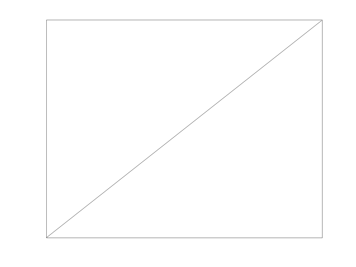
${{t_{2}=1/5}}$

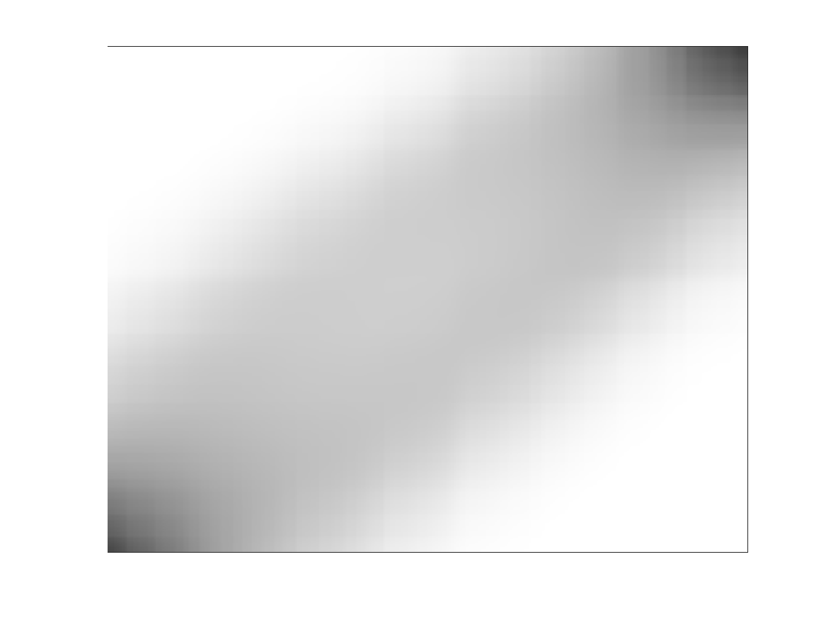
${{t_{3}=2/5}}$

${{t_{5}=3/5}}$

${{t_{5}=4/5}}$

${{t_{6}=1}}$

Figure 8: Joint measures $\boldsymbol{\Pi}_{1,k}$, $k=2,\cdots,5$ representing the movement of the particles from initial position $x\in[0,1]$ ($x$-axis) to position $x_{t_{k}}\in[0,1]$ ($y$-axis) at time $t_{k}$, where $\sigma(x)=1-x$. First row: Sinkhorn algorithm. Second row: NFFT-Sinkhorn algorithm.

${{t_{1}=0}}$

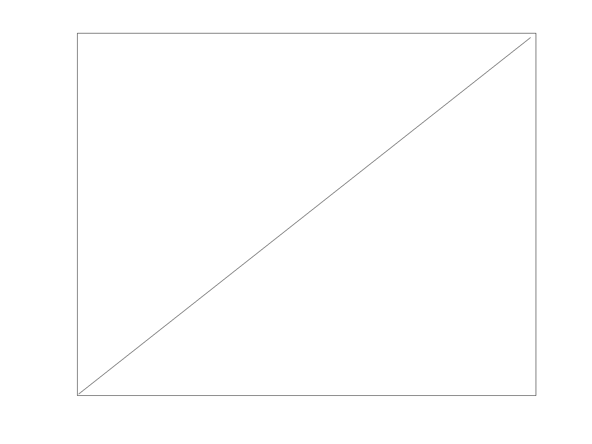
${{t_{2}=1/5}}$

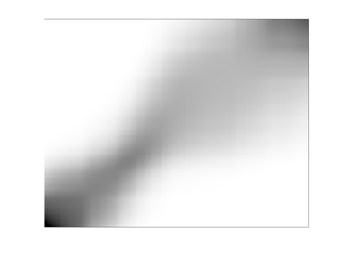
${{t_{3}=2/5}}$

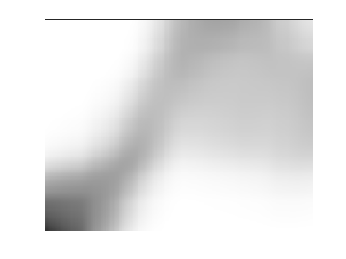
${{t_{4}=3/5}}$

${{t_{5}=4/5}}$

${{t_{6}=1}}$

Figure 9: Joint measures as in Figure 8, but with the function $\sigma(x)=\min(2x,1-2x)$.

7 Conclusions

We have proposed the NFFT-Sinkhorn algorithm to solve the $\text{MOT}_{\eta}$ problem efficiently. Assuming that the cost function of the multi-marginal optimal transport decouples according to a tree or a circle, we obtain a linear complexity in $K$. The complexity of the algorithm with respect to the numbers $n_{k},$ $k\in[K]$, of atoms of the discrete marginal measures is further improved by the non-uniform fast Fourier transform. This results in a considerable acceleration in our numerical experiments compared to the usual Sinkhorn algorithm. The tree-structured $\text{MOT}_{\eta}$ problem gives a much better numerical complexity than the circle-structured $\text{MOT}_{\eta}$ problem due to the fact that in the latter case, matrix–matrix products are required in Algorithm 3 instead of just matrix–vector products of Algorithm 2.

Acknowledgments

We gratefully acknowledge funding by the BMBF $01$|S$20053$B project SA$\ell$E. Furthermore, we gratefully acknowledge funding by the German Research Foundation DFG (STE 571/19-1, project number 495365311). We also thank the anonymous reviewers for making valuable suggestions to improve the article.

References

[1]
M. Agueh and G. Carlier.
Barycenters in the Wasserstein space.
SIAM J. Math. Anal., 43(2):904–924, 2011.
doi:10.1137/100805741.
[2]
M. Z. Alaya, M. Bérar, G. Gasso, and A. Rakotomamonjy.
Screening Sinkhorn algorithm for regularized optimal transport.
In Proceedings of the 33rd International Conference on Neural
Information Processing Systems, Red Hook, NY, USA, 2019. Curran Associates
Inc.
doi:10.5555/3454287.3455379.
[3]
D. Alfke, D. Potts, M. Stoll, and T. Volkmer.
NFFT meets Krylov methods: Fast matrix-vector products for the
graph Laplacian of fully connected networks.
Front. Appl. Math. Stat., 4(61), 2018.
doi:10.3389/fams.2018.00061.
[4]
J. M. Altschuler and E. Boix-Adsera.
Polynomial-time algorithms for multimarginal optimal
transport problems with structure.
Math. Program., in press, 2022.
doi:10.1007/s10107-022-01868-7.
[5]
H. Ammari, J. Garnier, and P. Millien.
Backpropagation imaging in nonlinear harmonic holography in the
presence of measurement and medium noises.
SIAM J. Imaging Sci., 7(1):239–276, 2014.
doi:10.1137/130926717.
[6]
F. Bassetti, S. Gualandi, and M. Veneroni.
On the computation of Kantorovich-Wasserstein distances between
2d-histograms by uncapacitated minimum cost flows.
2018.
arXiv:1804.00445.
[7]
F. Beier, J. von Lindheim, S. Neumayer, and G. Steidl.
Unbalanced multi-marginal optimal transport, 2021.
arXiv:2103.10854.
[8]
M. Beiglböck, C. Léonard, and W. Schachermayer.
A general duality theorem for the Monge-Kantorovich transport
problem.
Studia Math., 209:151–167, 2012.
URL: https://hal.archives-ouvertes.fr/hal-00515407.
[9]
J.-D. Benamou, G. Carlier, M. Cuturi, L. Nenna, and G. Peyré.
Iterative bregman projections for regularized transportation
problems.
SIAM J. Sci. Comput., 37(2):A1111–A1138, 2015.
doi:10.1137/141000439.
[10]
J.-D. Benamou, G. Carlier, and L. Nenna.
A numerical method to solve multi-marginal optimal transport problems
with Coulomb cost.
In Splitting methods in communication, imaging, science, and
engineering, Sci. Comput., pages 577–601. Springer, Cham, 2016.
[11]
J.-D. Benamou, G. Carlier, and L. Nenna.
Generalized incompressible flows, multi-marginal transport and
Sinkhorn algorithm.
Numer. Math., 142:33–54, 2019.
doi:10.1007/s00211-018-0995-x.
[12]
G. Beylkin.
On the fast Fourier transform of functions with singularities.
Appl. Comput. Harmon. Anal., 2:363–381, 1995.
doi:10.1006/acha.1995.1026.
[13]
M. Blondel, V. Seguy, and A. Rolet.
Smooth and sparse optimal transport.
In A. Storkey and F. Perez-Cruz, editors, Proceedings of the
Twenty-First International Conference on Artificial Intelligence
and Statistics, volume 84 of Proceedings of Machine Learning Research,
pages 880–889. PMLR, 2018.
[14]
N. Bonneel, G. Peyré, and M. Cuturi.
Wasserstein barycentric coordinates: Histogram regression using
optimal transport.
ACM Trans. Graph., 35(4), 2016.
doi:10.1145/2897824.2925918.
[15]
Y. Brenier.
The least action principle and the related concept of generalized
flows for incompressible perfect fluids.
J. Amer. Math. Soc., 2(2):225–255, 1989.
doi:10.2307/1990977.
[16]
Y. Brenier.
The dual least action problem for an ideal, incompressible fluid.
Archive for Rational Mechanics and Analysis, 122(4):323–351,
1993.
doi:10.1007/BF00375139.
[17]
Y. Brenier.
Minimal geodesics on groups of volume-preserving maps and generalized
solutions of the euler equations.
Comm. Pure Appl. Math, 52:411–452, 1997.
[18]
G. Carlier, A. Oberman, and E. Oudet.
Numerical methods for matching for teams and Wasserstein
barycenters.
ESAIM: M2AN, 49(6):1621–1642, 2015.
doi:10.1051/m2an/2015033.
[19]
M. Cuturi.
Sinkhorn distances: Lightspeed computation of optimal transport.
In C. J. C. Burges, L. Bottou, M. Welling, Z. Ghahramani, and K. Q.
Weinberger, editors, Advances in Neural Information Processing Systems,
volume 26. Curran Associates, Inc., 2013.
[20]
M. Cuturi and A. Doucet.
Fast computation of wasserstein barycenters.
In Proceedings of the 31st International Conference on
International Conference on Machine Learning - Volume 32, ICML’14, page
II–685–II–693. JMLR.org, 2014.
[21]
Y. Dolinsky and H. M. Soner.
Martingale optimal transport and robust hedging in continuous time.
Probab. Theory Related Fields, 160(1):391–427, 2014.
doi:10.1007/s00440-013-0531-y.
[22]
Y. Dolinsky and H. M. Soner.
Robust hedging with proportional transaction costs.
Finance Stoch., 18(2):327–347, 2014.
doi:10.1007/s00780-014-0227-x.
[23]
A. Dutt and V. Rokhlin.
Fast Fourier transforms for nonequispaced data II.
Appl. Comput. Harmon. Anal., 2:85–100, 1995.
doi:10.1137/0914081.
[24]
F. Elvander, I. Haasler, A. Jakobsson, and J. Karlsson.
Multi-marginal optimal transport using partial information with
applications in robust localization and sensor fusion.
Signal Process., 171, 2020.
doi:10.1016/j.sigpro.2020.107474.
[25]
R. Flamary, N. Courty, A. Gramfort, M. Z. Alaya, A. Boisbunon, S. Chambon,
L. Chapel, A. Corenflos, K. Fatras, N. Fournier, L. Gautheron, N. T. Gayraud,
H. Janati, A. Rakotomamonjy, I. Redko, A. Rolet, A. Schutz, V. Seguy, D. J.
Sutherland, R. Tavenard, A. Tong, and T. Vayer.
Pot: Python optimal transport.
J. Mach. Learn. Res., 22(78):1–8, 2021.
URL: http://jmlr.org/papers/v22/20-451.html.
[26]
U. Frisch, S. Matarrese, R. Mohayaee, and A. N. Sobolevski.
A reconstruction of the initial conditions of the universe by optimal
mass transportation.
Nature, 417:260–262, 2002.
doi:10.1038/417260a.
[28]
A. Genevay, M. Cuturi, G. Peyré, and F. Bach.
Stochastic optimization for large-scale optimal transport.
In Proceedings of the 30th International Conference on Neural
Information Processing Systems, page 3440–3448, Red Hook, NY, USA, 2016.
Curran Associates Inc.
doi:10.5555/3157382.3157482.
[29]
I. Haasler, A. Ringh, Y. Chen, and J. Karlsson.
Multimarginal optimal transport with a tree-structured cost and the
Schrödinger bridge problem.
SIAM J. Control Optim., 59(4):2428–2453, 2021.
doi:10.1137/20M1320195.
[30]
R. Hielscher and M. Quellmalz.
Optimal mollifiers for spherical deconvolution.
Inverse Problems, 31(8):085001, 2015.
doi:10.1088/0266-5611/31/8/085001.
[31]
L. Kantorovich.
On the translocation of masses.
Manag. Sci., 5(1):1–4, 1958.
[32]
J. Keiner, S. Kunis, and D. Potts.
Using NFFT3 - a software library for various nonequispaced fast
Fourier transforms.
ACM Trans. Math. Software, 36:Article 19, 1–30, 2009.
doi:10.1145/1555386.1555388.
[33]
P. Knopp and R. Sinkhorn.
Concerning connegative matrices and doubly stochastic matrices.
Pacific J. Math., 21(2):343 – 348, 1967.
doi:pjm/1102992505.
[34]
D. Koller and N. Friedman.
Probabilistic Graphical Models: Principles and Techniques.
Adaptive Computation and Machine Learning. The MIT Press, 2009.
[35]
R. Lakshmanan, A. Pichler, and D. Potts.
Fast Fourier transform boost for the Sinkhorn algorithm.
2022.
arXiv:2201.07524.
[36]
T. Lin, N. Ho, M. Cuturi, and M. I. Jordan.
On the complexity of approximating multimarginal optimal transport.
J. Mach. Learn. Res., 23:1–43, 2022.
URL: http://jmlr.org/papers/v23/19-843.html.
[37]
D. A. Lorenz, P. Manns, and C. Meyer.
Quadratically regularized optimal transport.
Appl. Math. Optim., 83(3):1919–1949, 2021.
doi:10.1007/s00245-019-09614-w.
[38]
S. D. Marino and A. Gerolin.
An optimal transport approach for the Schrödinger bridge
problem and convergence of Sinkhorn algorithm.
J. Sci. Comput., 85(2):27, 2020.
doi:10.1007/s10915-020-01325-7.
[39]
F. Nestler.
Parameter tuning for the NFFT based fast Ewald summation.
Front. Phys., 4(28), 2016.
doi:10.3389/fphy.2016.00028.
[40]
F. Nestler, M. Pippig, and D. Potts.
Fast Ewald summation based on NFFT with mixed periodicity.
J. Comput. Phys., 285:280–315, 2015.
[41]
S. Neumayer and G. Steidl.
From optimal transport to discrepancy.
In K. Chen, C.-B. Schönlieb, X.-C. Tai, and L. Younces, editors,
Handbook of Mathematical Models and Algorithms in Computer
Vision and Imaging: Mathematical Imaging and Vision, pages 1–36.
Springer, Cham, 2021.
doi:10.1007/978-3-030-03009-4_95-1.
[42]
B. Pass.
Multi-marginal optimal transport and multi-agent matching problems:
Uniqueness and structure of solutions.
Discrete Contin. Dyn. Syst., 34(4):1623–1639, 2014.
doi:10.3934/dcds.2014.34.1623.
[43]
B. Pass.
Multi-marginal optimal transport: Theory and applications.
ESAIM: M2AN, 49(6):1771–1790, 2015.
doi:10.1051/m2an/2015020.
[44]
G. Peyré and M. Cuturi.
Computational Optimal Transport: With Applications to Data
Science, volume 11.
Found. Trends Mach. Learn., 2019.
doi:10.1561/2200000073.
[45]
G. Plonka, D. Potts, G. Steidl, and M. Tasche.
Numerical Fourier Analysis.
Applied and Numerical Harmonic Analysis. Birkhäuser, 2018.
doi:10.1007/978-3-030-04306-3.
[46]
D. Potts and G. Steidl.
Fast summation at nonequispaced knots by NFFTs.
SIAM J. Sci. Comput., 24:2013–2037, 2003.
doi:10.1137/S1064827502400984.
[47]
D. Potts, G. Steidl, and A. Nieslony.
Fast convolution with radial kernels at nonequispaced knots.
Numer. Math., 98:329–351, 2004.
doi:10.1007/s00211-004-0538-5.
[48]
J. Rabin, G. Peyre, J. Delon, and M. Bernot.
Wasserstein barycenter and its application to texture mixing.
In A. M. Bruckstein, B. M. ter Haar Romeny, A. M. Bronstein, and
M. M. Bronstein, editors, Scale Space and Variational Methods in
Computer Vision, pages 435–446, Berlin, Heidelberg, 2012. Springer.
[49]
J. Solomon, F. de Goes, G. Peyré, M. Cuturi, A. Butscher, A. Nguyen, T. Du, L. Guibas.
Convolutional Wasserstein distances: efficient optimal transportation on geometric domains.
ACM Trans. Graph., 34(4):1–11, 2015.
doi:10.1145/2766963.
[50]
C. Strössner, D. Kressner.
Low-rank tensor approximations for solving multi-marginal optimal transport problems, 2022.
arXiv:2202.07340.
[51]
Y. Takezawa, R. Sato, Z. Kozareva, S. Ravi, and M. Yamada.
Fixed support tree-sliced Wasserstein barycenter, 2021.
arXiv:2109.03431.
[52]
G. Tartavel, G. Peyré, and Y. Gousseau.
Wasserstein loss for image synthesis and restoration.
SIAM J. Imaging Sci., 9(4):1726–1755, 2016.
doi:10.1137/16M1067494.
[53]
D. Terjék and D. González-Sánchez.
Optimal transport with -divergence regularization and generalized
Sinkhorn algorithm, 2021.
arXiv:2105.14337.
[54]
M. Thorpe, S. Park, S. Kolouri, G. K. Rohde, and D. Slepčev.
A transportation distance for signal analysis.
J. Math. Imaging Vision, 59(2):187–210, 2017.
doi:10.1007/s10851-017-0726-4.
[56]
T. Vogt and J. Lellmann.
Measure-valued variational models with applications to
diffusion-weighted imaging.
J. Math. Imaging Vis., 60(9):1482–1502, 2018.
doi:10.1007/s10851-018-0827-8.
[57]
J. von Lindheim.
Approximative algorithms for multi-marginal optimal transport and
free-support Wasserstein barycenters, 2022.
arXiv:2202.00954.