Efficient and Exact Multimarginal Optimal Transport with Pairwise Costs

Abstract

We address the numerical solution to multimarginal optimal transport (MMOT) with pairwise costs. MMOT, as a natural extension from the classical two-marginal optimal transport, has many important applications including image processing, density functional theory and machine learning, but lacks efficient and exact numerical methods. The popular entropy-regularized method may suffer numerical instability and blurring issues. Inspired by the back-and-forth method introduced by Jacobs and Léger, we investigate MMOT problems with pairwise costs. We show that such problems have a graphical representation and leverage this structure to develop a new computationally gradient ascent algorithm to solve the dual formulation of such MMOT problems. Our method produces accurate solutions which can be used for the regularization-free applications, including the computation of Wasserstein barycenters with high resolution imagery.

49Q22, 65K10, 49M29, 49N15, 90C35.

1 Introduction

Probability distributions are used throughout statistics, machine learning, and applied mathematics to model complex datasets and characterize uncertainty. Quantitatively comparing distributions and identifying structure in the space of probability distributions are therefore fundamental components of many modern algorithms for data analysis. Optimal transport (OT) provides a natural way of comparing two distributions by measuring how much effort is required to transform one distribution into another. The solution of an OT problem provides both a distance, called the Wasserstein distance, and a joint distribution, called the optimal coupling, which describes the optimal mass allocation between marginal distributions. Multi-marginal optimal transport (MMOT), which is the focus of this work, provides a generalization of classic OT to problems with more than two marginal distributions.

The field of OT has existed since Monge in the late 18th century, but has reemerged over the last few decades as a powerful theoretical and computational tool in many areas. Applications can be found in fields as diverse as chemistry and materials science [51, 20, 60], geophysics [61, 48], image processing [54, 9, 57], fluid dynamics [12, 8, 14], and machine learning [29, 17, 7, 34, 16], to name just a few. A key contributor to this surge is the development of efficient numerical methods for approximately solving OT problems. The concept of regularized optimal transport received renewed attention following [18], where an entropy regularization term is added to the original optimal transport problem, to form a matrix scaling problem that can be efficiently solved with Sinkhorn iterations [56]. The result is an easy-to-compute, albeit approximate, solution to the optimal transport problem.

Many refinements and extensions of regularized optimal transport have since been developed (e.g., [22, 19, 55]) including GPU-accelerated implementations [26], but the computational expense of these approaches can still become significant for small levels of entropic regularization. This makes such approaches intractable on quantitative applications where accurate approximations of the unregularized optimal coupling are required. For example, when the application demands maintaining the fluid dynamics interpretation of optimal transport [8], as it does in the sea ice velocity estimation problem of [48]. In addition, regularized formulations result in diffuse couplings that also cause blurring in image processing applications like barycentric interpolation [9]. A direct deblurring method like total variation reuglarizations may not recover ideal images [19].

The exact (unregularized) solution to OT is currently only feasible for certain subclasses of OT. OT on discrete measures is fundamentally an assignment problem and can be formulated as linear programming (LP). If the number of Dirac masses in the discrete measures is not too large, LP can be solved directly. Semi-discrete OT, where one measure is discrete and the other is continuous, is also naturally cast as an finite dimensional optimization problem (e.g., [45, 41]) and can often be solved exactly. Continuous OT problems, where both measures admit densities with respect to the Lebesgue measure, admit a PDE formulation based on the Monge-Ampère equation, which can be solved efficiently in 2 or 3 dimensions to obtain the OT solution [10]. The authors of [37] also provide an alternative method for OT with continuous distributions that can be represented on a uniform grid in $\mathbb{R}^{d}$. Their approach, called the “back-and-forth method” (BFM), lays the foundations for our MMOT solver and will be discussed in more detail in Section 2.4.

Similar to entropy regularized OT, there are regularized formulations of MMOT that admit approximate numerical solutions [9, 24, 35], following with complexity analysis [42, 25]. However, these approaches in general suffer the same numerical instability and blurring issues. Semidefinite relaxation to MMOT is proposed in [40] and provides as a lower bound to MMOT. The approach of [46] provides a regularization-free alternative for approximately solving MMOT problems with controllable levels of sub-optimality. However, the scalability of this approach to higher dimensional spaces with complex marginals is unclear. Authors of [3] also provide a LP-based polynomial-time algorithm to solve some MMOT with structure exactly, and graphical structure is one of them. They use the ellipsoid algorithm with an oracle related with $c$-transform (see Definition 2.2). The ellipsoid algorithm to LP is known to be slow in practice. Our goal is to construct a fast and exact (to within numerical tolerances) MMOT solver that can scale to marginal distributions derived from high resolution imagery. In practice, our method can be applied on MINST dataset, with more than 30 marginals and much more than 120 gridpoints, comparing the recently proposed GenCol method [28].

Contribution

In this paper, we develop and analyze a novel algorithm for the efficient solution of continuous MMOT problems with pairwise costs. More specifically, our method can deal with all cost function in a pairwise form $c(x_{1},\cdots,x_{m})=\sum_{i<j}c_{ij}(x_{i},x_{j})$, which includes most classical cost functions used in MMOT except the determinant form in [15]. In this category of cost functions, there is a natural graphical structure between marginals that our approach exploits to construct an efficient MMOT solver. In particular, inspired by the “back-and-forth” method of [37] for the classic two-marginal OT setting, we derive gradient updates and efficient $c$-transform routines that can be combined to solve the pairwise MMOT problem. The pushforward map, obtained as part of our computed MMOT solution, is accurate and can be utilized in regularizaiton-free applications, including denoising and the Wasserstein barycentric interpolation.

The paper is organized as follows. Section 2 consists of two parts. In the first part, we provide with all ingredients to understand the back-and-forth method (BFM). The concept of gradient in the Hilbert space is the key to BFM. In the second part, we introduce the MMOT problem with a focus on the duality theory, and basic graph theory for our description. In Section 3, we introduce the graphical representation of MMOT under assumptions (A1)–(A3), and develop the theory necessary to reformulate any MMOT of such type into an equivalent MMOT problem with a tree representation; this is encapsulated in Theorem 3.4. Section 4 introduces the main algorithm Algorithm 1 to solve any MMOT that has a tree representation. Numerical results with empirical convergence rates studies are presented in Section 5. Extensions to the Wasserstein barycenter problem are described in Section 5.3 as an important application of our methods. We close with concluding thoughts in Section 6.

2 Preliminaries

2.1 Two-Marginal Primal Formulation

The classic OT problem is a resource allocation problem. Given two Borel probability measures $\mu_{1},\mu_{2}$ on metric spaces $X_{1},X_{2}$ and a continuous cost function $c\mathrel{\mathop{\ordinarycolon}}X_{1}\times X_{2}\to[0,+\infty]$, the classic Monge OT problem is to find the cheapest way to transport $\mu_{1}$ to $\mu_{2}$:

(1) $$\inf_{T}\left\{\int c(x,T(x))\mathrm{d}\mu_{1}(x)\mathrel{\mathop{\ordinarycolon}}(T)_{\#}\mu_{1}=\mu_{2}\right\}.$$

Measures $\mu_{1}$ and $\mu_{2}$ are often referred as the source measure and the target measure, respectively. The transport map $T$ satisfies the push-forward condition $(T)_{\#}\mu_{1}=\mu_{2}$, which is shorthand notation for the condition that $\mu_{2}(A)=\mu_{1}(T^{-1}(A))$ for all Borel sets $A\subset X_{2}$. The optimal transport map $T^{*}$ is called the Monge map. The Monge map does not always exist. For example, if $\mu_{1}$ has fewer atoms than $\mu_{2}$, then mass from the same point in $X_{1}$ must be split to multiple points in $X_{2}$, which cannot be accomplished by any deterministic map $T$. Kantorovich provided a relaxation of (1) that circumvents this issue. The Kantorovich problem takes the form

(2) $$\inf\left\{\int_{X_{1}\times X_{2}}c(x_{1},x_{2})\mathrm{d}P(x_{1},x_{2})\mathrel{\mathop{\ordinarycolon}}P\in\Gamma(\mu_{1},\mu_{2})\right\},$$

where $\Gamma(\mu_{1},\mu_{2})$ is the set of transport plans defined by

$$\Gamma(\mu_{1},\mu_{2})=\left\{P\in\mathbb{P}(X_{1}\times X_{2})\mathrel{\mathop{\ordinarycolon}}(\pi_{1})_{\#}P=\mu_{1},~{}(\pi_{2})_{\#}P=\mu_{2}\right\},$$

and $\pi_{1},\pi_{2}$ are projections on each coordinate. The set of transport plans $\Gamma(\mu_{1},\mu_{2})$ consists of all joint probability measures on $X_{1}\times X_{2}$ with marginals $\mu_{1}$ and $\mu_{2}$. If no confusion may arise, we also use $P_{i}$ as shorthand notation for $(\pi_{i})_{\#}P$. When the source distribution $\mu_{1}$ is atomless, the transport plan $P^{\ast}$ solving the Kantorovich problem collapses onto the graph of the Monge solution and $P^{\ast}=(\mathop{}\mathopen{}\mathrm{id},T^{\ast})_{\#}\mu_{1}$, where $\mathop{}\mathopen{}\mathrm{id}\mathrel{\mathop{\ordinarycolon}}X_{1}\rightarrow X_{1}$ is the identity map (see [58]).

2.2 Two-Marginal Duality Theory

Instead of solving (2) directly, it is often more efficient to solve the dual form. From here on we will restrict our attention to spaces $X_{1}=X_{2}=\Omega\subset(\mathbb{R}^{d},\mathinner{\!\left\lvert\cdot\right\rvert}_{2})$ that are convex and compact, as well as costs in the form $c(x_{1},x_{2})=h(x_{1}-x_{2})$ for a strictly convex function $h\mathrel{\mathop{\ordinarycolon}}\mathbb{R}^{d}\mapsto\mathbb{R}$. Furthermore, we assume all marginals $(\mu_{i})$ are probability measures that are absolutely continuous with respect to the Lebesgue measure. Under these constraints, we have the following theorem.

Theorem 2.1 ([53], Theorem 1.40).

The dual problem to (2)

(3) $$\sup\left\{\int_{X_{1}}f_{1}\mathrm{d}\mu_{1}+\int_{X_{2}}f_{2}\mathrm{d}\mu_{2}\,\mathrel{\mathop{\ordinarycolon}}\,f_{1},f_{2}\in L^{1},f_{1}(x_{1})+f_{2}(x_{2})\leqslant c(x_{1},x_{2})\right\}$$

admits a $c$-conjugate solution $(f_{1},f_{2})$. That is, $f_{1}(x_{1})=\inf_{x_{2}}c(x_{1},x_{2})-f_{2}(x_{2})$ and $f_{2}(x_{2})=\inf_{x_{1}}c(x_{1},x_{2})-f_{1}(x_{1})$. (See Definition 2.2.) Furthermore, the strong duality between (2) and (3) holds.

As a result of strong duality, the maximal objective value in the dual problem (3) is equal to the minimum objective in the primal problem (2). For $c(x_{1},x_{2})=\mathinner{\!\left\lvert x_{1}-x_{2}\right\rvert}^{2}$, the optimal value is called as the Wasserstein distance $W^{2}_{2}(\mu_{1},\mu_{2})$.

As discussed in [5], because the optimal dual variables satisfy $f_{1}(x_{1})+f_{2}(x_{2})=c(x_{1},x_{2})$ on the support of the optimal coupling $P^{*}$, the Monge map can be recovered from the optimal dual solution $f_{1},f_{2}$ when the map exists. See Lemma A.3 and Theorem A.4 in the supplementary document.

2.3 $c$-Transform

The constraint in (3) induces a key concept in computational OT: the $c$-transform. The $c$-transform is a natural generalization of the more common Legendre-Fenchel transform $f^{*}(y)=\sup_{x}x\cdot y-f(x)$.

Definition 2.2 ($c$-transform).

The $c$-transform of a function $f\mathrel{\mathop{\ordinarycolon}}X_{1}\mapsto\mathbb{R}$ is given by

$$f^{c}(x_{2})=\inf_{x_{1}}c(x_{1},x_{2})-f(x_{1}).$$

In addition, we say that $f$ is $c$-concave if there exists a function $g\mathrel{\mathop{\ordinarycolon}}X_{2}\mapsto\mathbb{R}$ such that $f=g^{c}$. We say $(f_{1},f_{2})$ are $c$-conjugate if $f_{1}=f_{2}^{c}$ and $f_{2}=f_{1}^{c}$.

Remark 2.3.

The $c$-transform cannot decrease the objective value in (3). For any feasible dual variables $f_{1}$ and $f_{2}$, and any fixed point $x_{2}$, we have $f_{2}(x_{2})\leqslant c(x_{1},x_{2})-f_{1}(x_{1})$ for all $x_{1}$. This implies that $f_{2}(x_{2})\leqslant f_{1}^{c}(x_{2})$ and subsequently $\int_{X_{2}}f_{2}\mathrm{d}\mu_{2}\leqslant\int_{X_{2}}f_{1}^{c}\mathrm{d}\mu_{2}$.

Given $c(x_{1},x_{2})=h(x_{1}-x_{2})$ for some strictly convex function $h(\cdot)\mathrel{\mathop{\ordinarycolon}}\mathbb{R}^{d}\mapsto\mathbb{R}$, the map $S_{f}(x_{1})\mathrel{\ensurestackMath{\stackon[1pt]{=}{\scriptscriptstyle\Delta}}}x_{1}-\nabla h^{*}(\nabla f(x_{1}))$ will serve as a key ingredient in the classical OT theory. In particular, if $f=g^{c}$ for some continuous function $g$, then $S_{f}(x_{1})$ is the unique minimizer to $\inf_{x_{2}}c(x_{1},x_{2})-g(x_{2})$. Please refer to the supplemental document.

2.4 Gradient-based Optimization for OT

As a result of Remark 2.3 (also see Proposition 1.11 in [53]), the dual problem is equivalent to either of the following problems

(4a) $$\sup\left\{I_{1}(f_{1})=\int_{X_{1}}f_{1}\mathrm{d}\mu_{1}+\int_{X_{2}}f_{1}^{c}\mathrm{d}\mu_{2}\,\mathrel{\mathop{\ordinarycolon}}\,f_{1}\textrm{ is }c\textrm{-concave}\right\};$$

(4b) $$\sup\left\{I_{2}(f_{2})=\int_{X_{1}}f_{2}^{c}\mathrm{d}\mu_{1}+\int_{X_{2}}f_{2}\mathrm{d}\mu_{2}\,\mathrel{\mathop{\ordinarycolon}}\,f_{2}\textrm{ is }c\textrm{-concave}\right\},$$

whose maximizers are guaranteed to exist. Concavity and existence of a $c$-concave maximizer was proved by Brenier [13] for $c(x_{1},x_{2})=\frac{1}{2}\mathinner{\!\left\lvert x_{1}-x_{2}\right\rvert}^{2}$ and by Gangbo and McCann [31] for more general cost functions.

The concavity of (4) suggests that some gradient-based optimization could be effective at solving these problems. A gradient ascent step, for example, would take the form

(5) $$f^{(k+1)}=f^{(k)}+\sigma\nabla I(f^{(k)}),$$

where $f^{(k)}$ is the value of the dual variable at optimization iteration $k$, $\sigma\in\mathbb{R}$ is a step size parameter, and $\nabla I(f^{(k)})$ is a functional gradient of $I$ with respect to a dual variable $f$ (i.e., $f_{1}$ in (4a) or $f_{2}$ in (4b)). The Fréchet derivatives provide a mechanism for defining the gradient in a suitable Hilbert space.

Definition 2.4 (Fréchet derivatives and gradient in the Hilbert space).

Given a separable Hilbert space $(\mathcal{H},\mathinner{\!\left\lVert\cdot\right\rVert}_{\mathcal{H}})$ and a functional $E\mathrel{\mathop{\ordinarycolon}}\mathcal{H}\mapsto\mathbb{R}\cup\{+\infty\}$, we say a bounded linear operator $\delta E_{u}\mathrel{\mathop{\ordinarycolon}}\mathcal{H}\mapsto\mathbb{R}$ is the Fréchet derivative of $E$ at $u\in\mathcal{H}$ in the direction $v\in\mathcal{H}$ if

$$\lim_{\mathinner{\!\left\lVert v\right\rVert}_{\mathcal{H}}\to 0}\frac{\mathinner{\!\left\lvert E(u+v)-E(u)-\delta E_{u}(v)\right\rvert}}{\mathinner{\!\left\lVert v\right\rVert}_{\mathcal{H}}}=0.$$

The gradient $\nabla_{\mathcal{H}}E(u)\in\mathcal{H}$ is then defined as an element in the Hilbert space that can be used to compute any directional Fréchet derivative through an inner product. More specifically, we say $\nabla_{\mathcal{H}}E(u)$ is the Hilbert space gradient of $E$ at $u$ if

$$\langle\nabla_{H}E(u),v\rangle=\delta E_{u}(v),\qquad\textrm{for all }v\in\mathcal{H}.$$

Note that the choice of Hilbert space defines the inner product and thus the form of the gradient. Jacobs and Léger [37] show that for $c(x_{1},x_{2})=\frac{1}{2}\mathinner{\!\left\lvert x_{1}-x_{2}\right\rvert}^{2}$, guaranteeing the ascent of (5) requires that the space $\mathcal{H}$ cannot be weaker than

$$\dot{H}^{1}(\Omega)\mathrel{\ensurestackMath{\stackon[1pt]{=}{\scriptscriptstyle\Delta}}}\left\{u\mathrel{\mathop{\ordinarycolon}}\Omega\mapsto\mathbb{R}\,\mathrel{\mathop{\ordinarycolon}}\int_{\Omega}u\mathrm{d}x=0,\,\int_{\Omega}\mathinner{\!\left\lvert\nabla u(x)\right\rvert}^{2}\mathrm{d}x<\infty\right\},$$

with the inner product $\langle u_{1},u_{2}\rangle_{\dot{H}^{1}}=\int_{\Omega}\nabla u_{1}\cdot\nabla u_{2}\mathrm{d}x.$

Given a cost function $c(x_{1},x_{2})=h(x_{1}-x_{2})$ for some strictly convex function $h(\cdot)\mathrel{\mathop{\ordinarycolon}}\mathbb{R}^{d}\mapsto\mathbb{R}$, following techniques in [31, 32], Lemma 3 in [37] shows that the choice $\dot{H}^{1}$ results in the gradients:

(6) $$\nabla_{\dot{H}^{1}}I_{1}(f_{1}) =(-\Delta)^{-1}\left(\mu_{1}-(S_{f_{1}^{c}})_{\#}\mu_{2}\right);$$

$$\nabla_{\dot{H}^{1}}I_{2}(f_{2}) =(-\Delta)^{-1}\left(\mu_{2}-(S_{f_{2}^{c}})_{\#}\mu_{1}\right),$$

where $\Delta=\nabla\cdot\nabla$ is the Laplacian operator and the pushforward map $S_{f}(x)$ is given by

(7) $$S_{f}(x)\mathrel{\ensurestackMath{\stackon[1pt]{=}{\scriptscriptstyle\Delta}}}x-\nabla h^{*}(\nabla f(x)).$$

In fact, as shown by Brenier [13] for the quadratic cost and by Gangbo and McCann for strictly convex costs, the maximizer $(f_{1},f_{1}^{c})$ to (4a) (analogously with $(f_{2}^{c},f_{2})$ to (4b)) induces mappings $S_{f_{1}}$ and $S_{f_{1}^{c}}$ (analogously with $S_{f_{2}}$ and $S_{f_{2}^{c}}$), which satisfy

• $(S_{f_{1}})_{\#}\mu_{1}=\mu_{2}$ and $(S_{f_{1}^{c}})_{\#}\mu_{2}=\mu_{1}$;

• $S_{f_{1}}\mathrel{\mathop{\ordinarycolon}}X_{1}\mapsto X_{2}$ defines the unique minimizer to $\inf_{x_{2}}c(x_{1},x_{2})-f_{1}^{c}(x_{2})$; and $S_{f_{1}^{c}}\mathrel{\mathop{\ordinarycolon}}X_{2}\mapsto X_{1}$ defines the unique minimzer to $\inf_{x_{1}}c(x_{1},x_{2})-f_{1}(x_{1})$.

In this sense, formulas (6) are natural, as one may observe that $\mu_{1}=(S_{f_{1}^{c}})_{\#}\mu_{2}$ corresponds to the gradient being zero $\nabla_{\dot{H}^{1}}I_{1}(f_{1})=0\in\dot{H}^{1}$ and the inverse Laplacian $(-\Delta)^{-1}$ stemse from the inner product structure of the Hilbert space $\dot{H}^{1}$.

2.5 Multi-Marginal Primal Formulation

[50] provided a detailed theoretical survey about MMOT while here we just briefly introduce materials that we will use later. The primal MMOT problem takes the form

(8) $$\inf_{P\in\Gamma(\mu_{1},\cdots,\mu_{m})}\int_{\boldsymbol{X}}c(x_{1},\cdots,x_{m})\mathrm{d}P(x_{1},\cdots,x_{m}),$$

for the space $\boldsymbol{X}=X_{1}\times\cdots\times X_{m}$ and prescribed marginal probability measures $(\mu_{i})_{i=1}^{m}$. The set of transport plans $\Gamma(\mu_{1},\cdots,\mu_{m})$ is defined by

$$\Gamma(\mu_{1},\cdots,\mu_{m})\mathrel{\ensurestackMath{\stackon[1pt]{=}{\scriptscriptstyle\Delta}}}\left\{P\in\mathbb{P}(\boldsymbol{X})\mid(\pi_{i})_{\#}P=\mu_{i},1\leqslant i\leqslant m\right\}.$$

For simplicity, we will also denote the constraint by $P_{i}=\mu_{i}$ when the intent is clear. Analogously, the joint marginal $P_{ij}\mathrel{\ensurestackMath{\stackon[1pt]{=}{\scriptscriptstyle\Delta}}}(\pi_{ij})_{\#}P$ satisfies $\int_{X_{1}\times\cdots A_{i}\times\cdots A_{j}\times\cdots\times X_{m}}\mathrm{d}P=\int_{A_{i}\times A_{j}}\mathrm{d}P_{ij}$ for all Borel sets $A_{i}\subset X_{i}$ and $A_{j}\subset X_{j}$.

Cost functions vary in applications of MMOT. In density functional theory, costs of the form $c(x_{1},\cdots,x_{m})=\sum_{i<j}\mathinner{\!\left\lvert x_{i}-x_{j}\right\rvert}^{-1}$ or $c(x_{1},\cdots,x_{m})=\sum_{i<j}-\log\mathinner{\!\left\lvert x_{i}-x_{j}\right\rvert}$ arise (see [23]). Fluid dynamics use $c(x_{1},\cdots,x_{m})=\sum_{i=1}^{m-1}\tau^{-1}\mathinner{\!\left\lvert x_{i}-x_{i+1}\right\rvert}^{2}$ (see [12]). Wasserstein barycenters can be formulated as MMOTs with costs of the form $c(x_{1},\cdots,x_{m})=\sum_{1\leqslant i<j\leqslant m}\lambda_{i}\lambda_{j}|x_{i}-x_{j}|^{2}$ (see [32, 1, 33] and Section 5.3). An important feature of these costs is that they are all defined pairwise and fall into the form

$$c(x_{1},\ldots,x_{m})=\sum_{1\leqslant i<j\leqslant m}c_{ij}(x_{i},x_{j}).$$

Due to their broad applicability, such pairwise costs will be the focus of this work.

2.6 Multi-Marginal Duality Theory

Assume the cost function $c$ is continuous and each $\mu_{i}$ is supported on a convex and compact subset in $\mathbb{R}^{d}$. The dual problem corresponding to (8) is given by

(9) $$\sup_{(f_{1},\cdots,f_{m})}\sum_{i=1}^{m}\int_{X_{i}}f_{i}(x_{i})\mathrm{d}\mu_{i},$$

where $f_{i}\in L^{1}(\mu_{i})$ and $\sum_{i=1}^{m}f_{i}(x_{i})\leqslant c(x_{1},\cdots,x_{m})$. We call the optimal tuple $(f_{1},\cdots,f_{m})$ the Kantorovich potentials. On the opposite, in Section 4.1 for $m=2$ we call the optimal solution as the optimal loading/unloading prices in particular.

The concept of a $c$-splitting set extends the notion of a $c$-transform to the multi-marginal setting. A set $G\subset\boldsymbol{X}$ is a $c$-splitting set, if there exist $m$ functions $f_{i}\mathrel{\mathop{\ordinarycolon}}X_{i}\mapsto[-\infty,\infty)$ such that

$$\left\{\begin{aligned} &\sum_{i=1}^{m}f_{i}(x_{i})\leqslant c(x_{1},x_{2},\cdots,x_{m})\qquad\textrm{on}\quad X;\\ &\sum_{i=1}^{m}f_{i}(x_{i})=c(x_{1},x_{2},\cdots,x_{m})\qquad\textrm{in}\quad G.\end{aligned}\right.$$

These functions $(f_{1},f_{2},\cdots,f_{m})$ are called a $c$-splitting tuple.

Much like the $c$-transform was guaranteed to not decrease the dual objective in the two-marginal setting, for a $c$-splitting tuple $(f_{1},\cdots,f_{m})$, there exists a $c$-conjugate tuple $(\widetilde{f_{1}},\cdots,\widetilde{f_{m}})$ that does not decrease the dual objective. More specifically, for any $i$,

$$\widetilde{f_{i}}(x)=\left(\sum_{j\neq i}\widetilde{f_{j}}\right)^{c}\mathrel{\ensurestackMath{\stackon[1pt]{=}{\scriptscriptstyle\Delta}}}\inf_{\textrm{all~{}}y_{j}}c(y_{1},\cdots,y_{i-1},x,y_{i+1},\cdots,y_{m})-\sum_{j\neq i}\widetilde{f_{j}}(y_{j}),$$

is always a better candidate to (9). This is due to the fact that $f_{i}(x_{i})\leqslant\widetilde{f_{i}}(x_{i})$ for any $x_{i}\in X_{i}$. The $c$-conjugate tuple $(\widetilde{f_{1}},\widetilde{f_{2}},\cdots,\widetilde{f_{m}})$ can be constructed from:

$$\left\{\begin{aligned} \widetilde{f_{1}}(x)&=\inf_{\textrm{all~{}}y_{j}}c(x,y_{2},\cdots,y_{m})-\sum_{j\geqslant 2}f_{j}(y_{j});\\ \widetilde{f_{i}}(x)&=\inf_{\textrm{all~{}}y_{j}}c(y_{1},\cdots,y_{i-1},x,y_{i+1},\cdots,y_{m})-\sum_{j<i}\widetilde{f_{j}}(y_{j})-\sum_{j>i}f_{j}(y_{j}).\end{aligned}\right.$$

This is called a “convexification trick” in the context of convex analysis [15].

The existence of optimal solutions to (8) and (9), and the strong duality between these problems, was proved by [39] for more general cost functions. When $X_{i}=\mathbb{R}^{d}$, [15] also showed the existence of a $c$-conjugate optimal solution to (9) for general continuous cost functions. An extension of this result by [49] provides an important explicit connection between the primal and dual MMOT problems. Let $(\widetilde{f_{1}},\cdots,\widetilde{f_{m}})$ be a $c$-conjugate solution to the dual problem (9) and let $P$ be the optimal transport plan to primal problem (8), then we have the following connection between the primal solution and dual solution

$$\sum_{i=1}^{m}\widetilde{f}_{i}(x_{i})=c(x_{1},\cdots,x_{m})\qquad P\mathrm{-a.e.}.$$

2.7 Graph Theory

A graph $G=(V,E)$ is described by a set of nodes $V$ and a set of edges $E$. We will consider graphs where each node is associated with a marginal distribution $\mu_{i}$, or with a dual variable $f_{i}$, and will simply use the index $i$ to denote the node. An edge $e=(s,t)\in E$ from node $s$ to $t$ will then represent the pairwise cost $c_{st}(x_{s},x_{t})$. We will restrict our attention to simple graphs, which do not contain self-loops or multiple edges.

We will use both directed (where the order of the edge $(s,t)$ matters) and undirected graphs (where edges are order-agnostic). For directed graphs, we will use $N^{+}(i)=\{e_{t}\mathrel{\mathop{\ordinarycolon}}e\in E\text{ and }e_{s}=i\}$ and $N^{-}(i)\mathrel{\mathop{\ordinarycolon}}\{e_{s}\mathrel{\mathop{\ordinarycolon}}e\in E\text{ and }e_{t}=i\}$ to denote the sets of downstream nodes and upstream nodes neighboring node $i$, respectively. A particular type of graph called a tree will also be important to our approach. A tree is a graph where any two nodes are only connected by a single path. A rooted tree is a tree graph where all of the edges flow towards a single node, called the root. In a rooted tree with edges pointing towards root node $r$, the cardinality of the downstream set $|N^{+}(i)|=1$ for $i\neq r$ and $|N^{+}(r)|=0$.

3 Graphical Representation of MMOT

In Section 4 we will introduce a novel computational approach to solving MMOT problems with pairwise costs. A key component of that approach is the graphical representation of pairwise MMOT problems established below. This section also establishes one of our main theoretical results in Theorem 3.4: that any MMOT problem with pairwise cost can be represented as a rooted tree with nodes corresponding to marginal distributions and edges corresponding to pairwise costs.

While the duality theory described in Section 2.6 holds in more general settings, the rest of this paper will consider cost functions that satisfy the following three assumptions:

1. The cost function can be expressed as a sum of pairwise costs:

   $$c(x_{1},\cdots,x_{m})=\sum_{1\leqslant i<j\leqslant m}c_{ij}(x_{i},x_{j});$$

2. At least $(m-1)$ functions $c_{ij}(x_{i},x_{j})$ are not identically zero;

3. For each pair $(i,j)$, $c_{ij}(x_{i},x_{j})=h_{ij}(x_{i}-x_{j})$ for some strictly convex function $h_{ij}$.

The pairwise assumption (A1) causes the cost function to have a graph structure. The assumption (A2) ensures that the MMOT cannot be divided into multiple independent MMOT problems. Note that problems that do not satisfy the assumption (A2) can be trivially split into subproblems that do satisfy this assumption. The assumption (A3) enables a concise representation of the pushforward map (see discussions in Section 2.4 or Theorem A.4 in the supplemental document) and enables computationally efficient evaluations of $c_{ij}$-transforms. As a result of the general duality theory established by [39], under (A1)–(A3) the primal and dual MMOT problems in (8) and (9) both admit solutions, and strong duality holds.

The MMOT problem (8) under assumption (A1) is analogous to an undirected graph with $m$ nodes representing the marginals, and with edges for all costs $c_{st}(x_{s},x_{t})$ that are not identically $0$. This bijection is illustrated in Figure 1 for several MMOT problems.

As we show below in Section 4, MMOT problems that admit tree representations, like Figure 1(a), can be efficiently solved with a gradient-based optimization strategy generalized from the back-and-forth method of [37] for two-marginal OT problems. In Theorem 3.4 below, we show that the solution of MMOT problems without this tree structure (e.g., Figure 3(c) and Figure 1(c)) can be obtained through the solution of a larger “unrolled” problem that does exhibit this tree structure. This fundamental result allows us to apply our tree-based approach to any MMOT problem with pairwise costs.

for tree= edge = -, circle, minimum size=5mm, inner sep=0pt, draw, math content, tier/.wrap pgfmath arg=tier #1level(), anchor=center , [μ_1 [μ_2 [μ_3]] [μ_4]]

(a) $c=c_{12}+c_{23}+c_{14}$.

for tree= edge = -, circle, minimum size=5mm, inner sep=0pt, draw, math content, tier/.wrap pgfmath arg=tier #1level(), anchor=center , [μ_1 [μ_2 [,phantom] [μ_3, name=3] ] [μ_4, name=4] ] (4.south) – (3.north east);

(b) $c=c_{12}+c_{14}+c_{23}+c_{34}$.

for tree= edge = -, circle, minimum size=5mm, inner sep=0pt, draw, math content, tier/.wrap pgfmath arg=tier #1level(), anchor=center , [μ_1, name=1 [μ_2, name=2 [,phantom] [μ_3, name=3] ] [μ_4, name=4] ] (4.south) – (3.north east); (1.south) – (3.north); (2.east) – (4.west);

(c) $c=\sum_{i<j}c_{ij}$.

Figure 1: Undirected graphical representations of MMOT problems with $m=4$ marginals. (a) shows a cost that can be represented directly as a tree, whereas (b) and (c) are cyclic graphs. Theorem 3.4 provides a mechanism for unrolling these cyclic graphs in equivalent MMOT problems with tree structures. Also note that (c) shows the structure that arises in the MMOT formulation of Wasserstein barycenter problems.

The following lemma establishes a connection between the size of an MMOT problem with cyclic graph and the size of an equivalent problem with a tree structure.

Lemma 3.1.

Given an undirected graph $G=(V,E)$ with possible cycles, we need exactly $\mathinner{\!\left\lvert E\right\rvert}+1-\mathinner{\!\left\lvert V\right\rvert}$ duplicate nodes to be unrolled into a tree.

Proof 3.2.

Adding duplicate nodes and replacing original edges, the new graph retains the same number of edges while becoming a tree. A tree of $\mathinner{\!\left\lvert E\right\rvert}$ edges has $\mathinner{\!\left\lvert E\right\rvert}+1$ nodes. Thus we need to add $\mathinner{\!\left\lvert E\right\rvert}+1-\mathinner{\!\left\lvert V\right\rvert}$ duplicate nodes.

To show that solving any pairwise MMOT is equivalent to solving another MMOT with a tree representation, we will need the following generalized gluing lemma.

Lemma 3.3 (Generalized gluing lemma, Theorem A.1 in [21]).

Let $J$ be an arbitrary index set and for each $j\in J$, let $X_{j},Y_{j}$ be Polish spaces and $\boldsymbol{X}=\Pi_{j\in J}X_{j},\boldsymbol{Y}=\Pi_{j\in J}Y_{j}$. Let $\phi_{j}\mathrel{\mathop{\ordinarycolon}}X_{j}\mapsto Y_{j}$ be a measurable map and let $\mu_{j}\in\mathbb{P}(X_{j})$. Let $Q\in\mathbb{P}(\boldsymbol{Y})$ such that $(\phi_{j})_{\#}\mu_{j}=(\mathbf{Proj}_{j})_{\#}Q$ for all $j\in J$.

Then there exists a $P\in\mathbb{P}(\boldsymbol{X})$ such that:

$$\left\{\begin{aligned} &(\mathbf{Proj}_{j})_{\#}P=\mu_{j},\qquad\textrm{for all }j\in J;\\ &\left(\left(\phi_{j}\circ\mathbf{Proj}_{j}\right)_{j\in J}\right)_{\#}{P}=Q.\end{aligned}\right.$$

We are now ready to show that any pairwise MMOT problem can be “unrolled” into an equivalent MMOT problem with a tree structure. Qualitatively, the process of unrolling a graph is illustrated in Figure 2, where a single cycle is broken by duplicating the marginal $\mu_{4}$. This process is made more precise in Theorem 3.4.

Theorem 3.4.

Given a cost function $c(x_{1},\cdots,x_{m})$ satisfying assumptions (A1), (A2) and (A3) that corresponds to an undirected graph $G=(V,E)$ with possible cycles, let $n=\mathinner{\!\left\lvert E\right\rvert}+1$.

1. There exists a map: $\bar{T}\mathrel{\mathop{\ordinarycolon}}X_{1}\times\dots\times X_{m}\mapsto X_{1}\times\dots\times X_{n}$ such that for the cost function $\bar{c}(x_{1}\cdots,x_{n})$ on $X_{1}\times\dots\times X_{n}$ with $c=\bar{c}\circ\bar{T}$, which corresponds to an undirected tree $\bar{G}=(\bar{V},\bar{E})$ with $\mathinner{\!\left\lvert\bar{E}\right\rvert}=\mathinner{\!\left\lvert E\right\rvert}=n-1$ and $\mathinner{\!\left\lvert\bar{V}\right\rvert}=n$, and we have

   (10) $$\inf_{P^{(m)}\in\Gamma(\mu_{1},\cdots,\mu_{m})}\int c(x_{1},\cdots,x_{m})\mathrm{d}P^{(m)}=\inf_{P^{(n)}\in\mathcal{Q}^{(n)}_{2}}\int\bar{c}(x_{1},\cdots,x_{n})\mathrm{d}P^{(n)},$$

   where $\mathcal{Q}^{(n)}_{2}=\left\{Q=(\bar{T})_{\#}P\in\mathbb{P}(X_{1}\times\cdots\times X_{n})\mid P\in\Gamma(\mu_{1},\cdots,\mu_{m})\right\}$

2. Let $P^{(m)}$ and $(f_{i})_{i=1}^{m}$ be the optimal primal and dual solutions to the original MMOT (8) and (9), and let $P^{(n)}$ and $(\bar{f}_{i})_{i=1}^{m}$ be the optimal primal and dual solutions to the new MMOT:

   (11) $$\inf_{P^{(n)}\in\Gamma(\mu_{1},\cdots,\mu_{n})}\int\bar{c}(x_{1},\cdots,x_{n})\mathrm{d}P^{(n)};$$

   $$\sup_{\bar{f}_{1}+\cdots+\bar{f}_{n}\leqslant\bar{c}}\sum_{i=1}^{n}\int\bar{f}_{i}(x_{i})\mathrm{d}\mu_{i},$$

   where $(\mu_{k})_{k=m+1}^{n}$ are duplicated from $(\mu_{i})_{i=1}^{m}$ in the unrolling process (shown in Fig. 2 as an illustration). Then the new MMOT provides a lower bound to the original MMOT, that is:

   (12) $$\inf_{P^{(m)}\in\Gamma(\mu_{1},\cdots,\mu_{m})}\int c\mathrm{d}P^{(m)}= \sup_{f_{1}+\cdots+f_{m}\leqslant c}\sum_{i=1}^{m}\int f_{i}(x_{i})\mathrm{d}\mu_{i}$$

   $$\geqslant \sup_{\bar{f}_{1}+\cdots+\bar{f}_{n}\leqslant\bar{c}}\sum_{i=1}^{n}\int\bar{f}_{i}(x_{i})\mathrm{d}\mu_{i}$$

   $$= \inf_{P^{(n)}\in\Gamma(\mu_{1},\cdots,\mu_{n})}\int\bar{c}\mathrm{d}P^{(n)}.$$

3. Assume all $c_{ij}$ and the optimal dual solutions are $C^{2,\alpha}$, then the equality in (12) holds. That is, solving the original MMOT is equivalent to solve the new MMOT. Furthermore, for any $i$, the original optimal dual solution $f_{i}$ is the sum of all $\bar{f}_{j}$ whose nodes are duplicated from $\mu_{i}$.

Figure 2: Breaking one cycle in the left graph results in the right graph with an additional node. Theorem 3.4 repeats this process to obtain an equivalent MMOT with a tree structure.

Proof 3.5.

We prove it by iteration. Assume there is a cycle in $G=(V,E)$ and we can remove an edge $e=(i,j)$ to break the cycle. Let $c(x_{1},\cdots,x_{m})=c_{ij}(x_{i},x_{j})+d(x_{1},\cdots,x_{m})$ and $\widetilde{c}(x_{1},\cdots,x_{m+1})=c_{ij}(x_{i},x_{m+1})+d(x_{1},\cdots,x_{m})$. By defining a map: $T\mathrel{\mathop{\ordinarycolon}}X_{1}\times\cdots\times X_{m}\mapsto X_{1}\times\cdots\times X_{m}\times X_{m+1}$ with $X_{m+1}=X_{j}$, given by $T(x_{1},\cdots,x_{j},\cdots,x_{m})=(x_{1},\cdots,x_{j},\cdots,x_{m},x_{j})$, we note that: $c=\widetilde{c}\circ T$, thus for any $P\in\mathbb{P}(X_{1}\times\cdots\times X_{m})$, we have

(13) $$\int c(x_{1},\cdots,x_{m})\mathrm{d}P=\int\widetilde{c}\circ T\mathrm{d}P=\int\widetilde{c}\mathrm{d}[(T)_{\#}P].$$

Note that this unrolling process preserves the number of edges, thus repeat this process and one can obtain the map $\bar{T}$ and the cost function $\bar{c}(x_{1},\cdots,x_{n})$ that corresponds to an undirected tree $\bar{G}=(\bar{V},\bar{E})$ with $\mathinner{\!\left\lvert\bar{E}\right\rvert}=n-1$ and $\mathinner{\!\left\lvert\bar{V}\right\rvert}=n$. By change of variables, we prove the part (a):

$$\inf_{P^{(m)}\in\Gamma(\mu_{1},\cdots,\mu_{m})}\int c(x_{1},\cdots,x_{m})\mathrm{d}P^{(m)}=\inf_{P^{(n)}\in\mathcal{Q}^{(n)}_{2}}\int\bar{c}(x_{1},\cdots,x_{n})\mathrm{d}P^{(n)}.$$

Now, we go back to unroll for one step and prove part (b) by iteration. Consider the following two subsets $\mathcal{Q}_{1},\mathcal{Q}_{2}$ of couplings in $\mathbb{P}(X_{1}\times\cdots\times X_{m}\times X_{j})$, where

$$\mathcal{Q}_{1}=\left\{Q\mid Q_{i}=\mu_{i}\textrm{ for all }i\notin\{j,m+1\};Q_{j,m+1}=((\mathop{}\mathopen{}\mathrm{id},\mathop{}\mathopen{}\mathrm{id}))_{\#}\mu_{j}\right\},$$

$$\mathcal{Q}_{2}=\left\{Q=(T)_{\#}P\in\mathbb{P}(X_{1}\times\cdots\times X_{m}\times X_{j})\mid P\in\Gamma(\mu_{1},\cdots,\mu_{m})\right\}.$$

Recall $Q_{i}$ is the shorthand notation for $(\pi_{i})_{\#}Q$, analogously with $Q_{j,m+1}$.

We first show that these two sets are equivalent.

For a coupling $Q\in\mathcal{Q}_{2}$, when $i\notin\{j,m+1\}$ and for any Borel sets $A_{i}$ in $X_{i}$, we have

$$Q_{i}(A_{i})=(\pi_{i})_{\#}Q(A_{i})=(\pi_{i})_{\#}((T)_{\#}P)(A_{i})=P(T^{-1}\circ\pi_{i}^{-1}(A_{i}))=\mu_{i}(A_{i}).$$

Also, for any Borel sets $A_{j}$ in $X_{j}$ and $A_{m+1}$ in $X_{m+1}=X_{j}$:

$$Q_{j,m+1}(A_{j}\times A_{m+1}) =((\pi_{j},\pi_{m+1}))_{\#}Q(A_{j}\times A_{m+1})$$

$$=P(T^{-1}\circ(\pi_{j},\pi_{m+1})^{-1}(A_{j}\times A_{m+1}))$$

$$=P(T^{-1}(X_{1}\times\cdots\times A_{j}\times X_{j+1}\times\cdots\times X_{m}\times A_{m+1}))$$

$$=P(X_{1}\times\cdots\times(A_{j}\cap A_{m+1})\times\cdots\times X_{m})$$

$$=\mu_{j}(A_{j}\cap A_{m+1})=((\mathop{}\mathopen{}\mathrm{id},\mathop{}\mathopen{}\mathrm{id}))_{\#}\mu_{j}(A_{j}\times A_{m+1}).$$

Thus $Q\in\mathcal{Q}_{1}$, showing that $\mathcal{Q}_{2}\subseteq\mathcal{Q}_{1}$.

On the other hand, consider a coupling $Q\in\mathcal{Q}_{1}$. Comparing with Lemma 3.3, we have $(X_{i},\mu_{i})$, take $Y_{i}=X_{i}$ for $i\neq j$ and $Y_{j}=X_{j}\times X_{m+1}$ with $X_{m+1}=X_{j}$, thus $\boldsymbol{Y}=X_{1}\times\cdots\times(X_{j}\times X_{m+1})\times\cdots X_{m}$. For $i\neq j$, define $\phi_{i}=\mathop{}\mathopen{}\mathrm{id}\mathrel{\mathop{\ordinarycolon}}X_{i}\mapsto Y_{i}$ and $\phi_{j}\mathrel{\mathop{\ordinarycolon}}X_{j}\mapsto Y_{j}$ by $\phi_{j}=(\mathop{}\mathopen{}\mathrm{id},\mathop{}\mathopen{}\mathrm{id})$. Up to a permutation, we treat $Q\in\mathbb{P}(X_{1}\times\cdots\times X_{m}\times X_{j})$ as $Q\in\mathbb{P}(\boldsymbol{Y})$, thus by the definition of $\mathcal{Q}_{1}$, we have:

$$(\phi_{i})_{\#}\mu_{i}=(\textbf{Proj}_{i})_{\#}Q;\qquad\textrm{and}\qquad((\mathop{}\mathopen{}\mathrm{id},\mathop{}\mathopen{}\mathrm{id}))_{\#}\mu_{j}=(\textbf{Proj}_{j})_{\#}Q$$

Thanks to Lemma 3.3, there exists a $P\in\mathbb{P}(\boldsymbol{X})$ such that:

$$\left\{\begin{aligned} &(\textbf{Proj}_{i})_{\#}P=\mu_{i}\qquad\textrm{for all }i;\\ &((\phi_{1}\circ\textbf{Proj}_{1},\cdots,\phi_{j}\circ\textbf{Proj}_{j},\cdots,\phi_{m}\circ\textbf{Proj}_{m}))_{\#}P=Q.\end{aligned}\right.$$

Note that

$$(\phi_{1}\circ\textbf{Proj}_{1},\cdots,\phi_{j}\circ\textbf{Proj}_{j},\cdots,\phi_{m}\circ\textbf{Proj}_{m})(x_{1},\cdots,x_{j},\cdots,x_{m})$$

$$= (\phi_{1}(x_{1}),\cdots,\phi_{j}(x_{j}),\cdots,\phi_{m}(x_{m}))=(x_{1},\cdots,(x_{j},x_{j}),\cdots,x_{m}),$$

which is a permutation of $T$. As we prove the existence of $P\in\Gamma(\mu_{1},\cdots,\mu_{m})$, thus $Q\in\mathcal{Q}_{2}$ and subsequently $\mathcal{Q}_{1}\subseteq\mathcal{Q}_{2}$. Combined with the discussion above, this implies that $\mathcal{Q}_{1}=\mathcal{Q}_{2}$.

Using this equivalence and (13) results in

$$\inf_{P}\int c(x_{1},\cdots,x_{m})\mathrm{d}P=\inf_{Q\in\mathcal{Q}_{2}}\int\widetilde{c}(x_{1},\cdots,x_{m+1})\mathrm{d}Q=\inf_{Q\in\mathcal{Q}_{1}}\int\widetilde{c}(x_{1},\cdots,x_{m+1})\mathrm{d}Q.$$

On one hand, by Section 2.6 we have the strong duality for the original MMOT under the cost $c(x_{1},\cdots,x_{m})$:

(14) $$\inf_{P\in\Gamma(\mu_{1},\cdots,\mu_{m})}\int c(x_{1},\cdots,x_{m})\mathrm{d}P=\sup_{f_{1}+\cdots+f_{m}\leqslant c}\sum_{i=1}^{m}\int f_{i}(x_{i})\mathrm{d}\mu_{i}.$$

On the other hand, we also have the strong duality for the new MMOT under the cost $\widetilde{c}(x_{1},\cdots,x_{m+1})$ for $\mu_{m+1}=\mu_{j}$:

(15) $$\inf_{Q\in\Gamma(\mu_{1},\cdots,\mu_{m},\mu_{m+1})}\int\widetilde{c}(x_{1},\cdots,x_{m+1})\mathrm{d}Q=\sup_{\widetilde{f}_{1}+\cdots+\widetilde{f}_{m+1}\leqslant\widetilde{c}}\sum_{i=1}^{m+1}\int\widetilde{f}_{i}(x_{i})\mathrm{d}\mu_{i}.$$

Due to the fact that $\mathcal{Q}_{1}\subset\Gamma(\mu_{1},\cdots,\mu_{m},\mu_{j})$, we have:

$$\inf_{P}\int c\mathrm{d}P=\inf_{Q\in\mathcal{Q}_{1}}\int\widetilde{c}(x_{1},\cdots,x_{m+1})\mathrm{d}Q\geqslant\inf_{Q\in\Gamma(\mu_{1},\cdots,\mu_{m},\mu_{j})}\int\widetilde{c}(x_{1},\cdots,x_{m+1})\mathrm{d}Q.$$

By iterating the unrolling from $m+1$ nodes to $n$ nodes, we prove the part (b).

The characteristic function of the set $\mathcal{Q}_{1}$ is given by:

$$\sup_{\widetilde{f}_{i}}\sum_{i\not\in\left\{j,m+1\right\}}\int_{X_{i}}\widetilde{f}_{i}\mathrm{d}\mu_{i}-\int_{X_{1}\times\cdots\times X_{m}\times X_{m+1}}\left(\sum_{i\not\in\left\{j,m+1\right\}}\widetilde{f}_{i}(x_{i})\right)\mathrm{d}Q$$

$$+\sup_{g}\int_{X_{j}\times X_{m+1}}g(x_{j},x_{m+1})\mathrm{d}[((\mathrm{id},\mathrm{id}))_{\#}\mu_{j}]-\int_{X_{1}\times\cdots\times X_{m}\times X_{m+1}}g(x_{j},x_{m+1})\mathrm{d}Q$$

$$= \left\{\begin{aligned} &0\qquad&Q\in\mathcal{Q}_{1};\\ &+\infty\qquad&Q\in\mathcal{M}_{+}(X_{1}\times\dots\times X_{m}\times X_{m+1})\backslash\mathcal{Q}_{1}.\end{aligned}\right.$$

among all bounded and continuous functions $\widetilde{f}_{i}\in C_{b}(X_{i})$ and $g\in C_{b}(X_{j}\times X_{m+1})$ for $X_{m+1}=X_{j}$. By noting that

$$\int_{X_{j}\times X_{m+1}}g(x_{j},x_{m+1})\mathrm{d}[((\mathrm{id},\mathrm{id}))_{\#}\mu_{j}]=\int_{X_{j}}g(x_{j},x_{j})\mathrm{d}\mu_{j},$$

we write the following into the Lagrangian form:

$$\inf_{Q\in\mathcal{Q}_{1}}\int\widetilde{c}(x_{1},\cdots,x_{m+1})\mathrm{d}Q$$

$$= \inf_{Q}\int\widetilde{c}\mathrm{d}Q+\sup_{\widetilde{f}_{i},g}\sum_{i\not\in\left\{j,m+1\right\}}\int\widetilde{f}_{i}\mathrm{d}\mu_{i}+\int g\mathrm{d}[((\mathrm{id},\mathrm{id}))_{\#}\mu_{j}]-\int(g+\sum_{i\not\in\left\{j,m+1\right\}}\widetilde{f}_{i})\mathrm{d}Q$$

(16) $$= \left\{\begin{aligned} &\sup_{\widetilde{f}_{i},g}\sum_{i\not\in\left\{j,m+1\right\}}\int_{X_{i}}\widetilde{f}_{i}\mathrm{d}\mu_{i}+\int_{X_{j}}g(x_{j},x_{j})\mathrm{d}\mu_{j}\\ &\textrm{s.t~{}}\sum_{i\not\in\left\{j,m+1\right\}}\widetilde{f}_{i}(x_{i})+g(x_{j},x_{m+1})\leqslant\widetilde{c}(x_{1},\cdots,x_{m+1})\end{aligned}\right.$$

When $g(x_{j},x_{m+1})$ is a additively separable function, that is, there exists bounded continuous function $\widetilde{f}_{j},\widetilde{f}_{m+1}$ such that $g(x_{j},x_{m+1})=\widetilde{f}_{j}(x_{j})+\widetilde{f}_{m+1}(x_{m+1})$, then (3.5) turns to be the new MMOT (15). Once again, we see that the new MMOT is a lower bound.

For the optimal $Q\in\mathcal{Q}_{1}$ and the optimal dual solution $(g,\widetilde{f}_{1},\cdots,\widetilde{f}_{m})$, we have:

$$\sum_{i\not\in\left\{j,m+1\right\}}\widetilde{f}_{i}(x_{i})+g(x_{j},x_{m+1})=\widetilde{c}(x_{1},\cdots,x_{m+1})=d(x_{1},\cdots,x_{m})+c_{ij}(x_{i},x_{m+1}),$$

$Q$-almost everywhere. That is:

$$g(x_{j},x_{m+1})=d(x_{1},\cdots,x_{m})+c_{ij}(x_{i},x_{m+1})-\sum_{i\not\in\left\{j,m+1\right\}}\widetilde{f}_{i}(x_{i})\qquad\textrm{a.e.~{}}Q.$$

Due to the additional assumption on the differentiability in the part (c), we note that the mixed partial derivatives $\frac{\partial^{2}}{\partial x_{j}\partial x_{m+1}}$ are zero on the right hand side, thus at the optimality, $g(x_{j},x_{m+1})$ is additively separable. Therefore, by (14), (15) and (3.5), we have:

(17) $$\inf_{P}\int c\mathrm{d}P =\inf_{Q\in\mathcal{Q}_{1}}\int\widetilde{c}(x_{1},\cdots,x_{m+1})\mathrm{d}Q$$

$$=\sup_{g+\widetilde{f}_{1}+\cdots+\widetilde{f}_{m}\leqslant\widetilde{c}(x_{1},\cdots,x_{m+1})}\sum_{i\not\in\left\{j,m+1\right\}}\int_{X_{i}}\widetilde{f}_{i}\mathrm{d}\mu_{i}+\int_{X_{j}}g(x_{j},x_{j})\mathrm{d}\mu_{j}$$

$$=\sup_{\widetilde{f}_{1}+\cdots+\widetilde{f}_{m+1}\leqslant\widetilde{c}}\sum_{i=1}^{m+1}\int_{X_{i}}\widetilde{f}_{i}\mathrm{d}\mu_{i}$$

$$=\inf_{Q\in\Gamma(\mu_{1},\cdots,\mu_{m},\mu_{j})}\int\widetilde{c}(x_{1},\cdots,x_{m+1})\mathrm{d}Q.$$

which sets up the equivalence between the original MMOT and the new MMOT.

Furthermore, let $(f_{i})_{i=1}^{m}$ and $(\widetilde{f}_{i})_{i=1}^{m+1}$ be the Kantorovich potentials. Due to (14), (15) and (17), we have

$$\sum_{i=1}^{m}\int_{X_{i}}f_{i}\mathrm{d}\mu_{i}=\sum_{i=1}^{m+1}\int_{X_{i}}\widetilde{f}_{i}\mathrm{d}\mu_{i}=\sum_{i\notin\left\{j,m+1\right\}}\int_{X_{i}}\widetilde{f}_{i}\mathrm{d}\mu_{i}+\int_{X_{j}}(\widetilde{f}_{j}(x_{j})+\widetilde{f}_{m+1}(x_{j}))\mathrm{d}\mu_{j}.$$

Therefore we can define an optimal dual solution $(f_{i})_{i=1}^{m}$ to the original problem, in terms of the optimal dual solution to the new problem:

$$\left\{\begin{aligned} &f_{i}=\widetilde{f}_{i},\qquad&i\neq j;\\ &f_{j}=\widetilde{f}_{j}+\widetilde{f}_{m+1}\qquad&i=j.\end{aligned}\right.$$

The above process can be repeated to remove all cycles in the tree. Lemma 3.1 guarantees that only a finite number or repetitions are required, thus completing the proof.

Remark 3.6.

As the regularity theory of the Kantorovich potentials is in general subtle (see Section 6.2 in [6] for example), we impose a strong assumption on the potentials directly in the part (c), in order to obtain the equivalence. For the cost $c_{ij}(x_{i},x_{j})=\mathinner{\!\left\lvert x_{i}-x_{j}\right\rvert}^{2}$, by the Caffarelli’s regularity theory, the Kantorovich potentials are $C^{2,\alpha}$ and thus the additional assumption in the part (c) is relieved. We would like to seek for necessary conditions or weaker sufficient conditions on the cost function for the equivalence in the future work.

4 Computational Approach

To solve the MMOT problem, we need to maximize the dual functional

(18) $$I(f_{1},\cdots,f_{m})=\sum_{i=1}^{m}\int f_{i}\mathrm{d}\mu_{i}$$

among dual variables satisfying $\sum_{i=1}^{m}f_{i}(x_{i})\leqslant c(x_{1},\cdots,x_{m})$. Similar to the two-marginal approach of [37], by leveraging $c$-transform to get rid of the constraint, we will use gradient ascent on the remaining $(m-1)$ dual variables in the space $\dot{H}^{1}$. As shown below, the graphical interpretation of the MMOT problem will enable fast $c$-transforms and gradient updates.

On a high level, our algorithm consists of three steps:

1. We first construct an undirected graph with possible cycles based on the cost function.

2. We follow Theorem 3.4 and “unroll” the cyclic graph into an undirected tree, at the cost of adding duplicate nodes.

3. We solve the unrolled problem with the gradient ascent steps described in Section 4.

We have discussed Steps I and II in Section 3. As illustrated in Figure 3, by picking an arbitrary node as the root node and traversing the undirected tree with a breadth first search to add directionality, we obtain a directed rooted tree. Our primary computational task in this section is then finding the solution to MMOT problems with tree representations.

for tree= edge = stealth-, circle, minimum size=5mm, inner sep=0pt, draw, math content, tier/.wrap pgfmath arg=tier #1level(), anchor=center , [f_1,name=L0, [f_2,name=L1,[f_3,name=L2]], [f_4]] et 1 = (L0) in node at (1.5,1) $L˙1=0$; et 1 = (L1) in node at (1.9,1) $L˙2=L˙4=1$; et 1 = (L2) in node at (1.5,1) $L˙3=2$;

(a) Tree variant of (Figure 1(a)) with root note $f˙1$.

for tree= edge = stealth-, circle, minimum size=5mm, inner sep=0pt, draw, math content, tier/.wrap pgfmath arg=tier #1level(), anchor=center , [f˙4,name=L0, [f˙1, name=L1, [f˙2,name=L2, [f˙3, name=L3]] ] ] et 1 = (L0) in node at (1.5,1) $L˙4=0$; et 1 = (L1) in node at (1.5,1) $L˙1=1$; et 1 = (L2) in node at (1.5,1) $L˙2=2$; et 1 = (L3) in node at (1.5,1) $L˙3=3$;

(b) Another tree variant of (Figure 1(a)) with root node $f˙4$.

% % % for tree= % edge = -, % circle, % minimum size=5mm, % inner sep=0pt, % draw, % math content, % tier/.wrap pgfmath arg=tier #1level(), % anchor=center % , % [μ˙1 % [μ˙2 % [,phantom] % [μ˙3, name=3] % ] % [μ˙4, name=4] % ] % (4.south) – (3.north east); % . % %

(c) Undirected graph corresponding to cost function $c=c˙12+c˙14+c˙23+c˙34$.

for tree= edge = -, circle, minimum size=5mm, inner sep=0pt, draw, math content, tier/.wrap pgfmath arg=tier #1level(), anchor=center , [μ˙1 [μ˙2 [μ˙3] ] [μ˙4, [μ˙3]] ]

(d) Unrolled variant of (Figure 3(c)) obtained by duplicating $μ˙3$.

for tree= edge = stealth-, circle, minimum size=5mm, inner sep=0pt, draw, math content, tier/.wrap pgfmath arg=tier #1level(), anchor=center , [f˙1,name=L0, [f˙2,[f˙3]], [f˙4, name=L1, [f˙5,name=L2]]] et 1 = (L0) in node at (1.5,1) $L˙1=0$; et 1 = (L1) in node at (1.9,1) $L˙2=L˙4=1$; et 1 = (L2) in node at (1.9,1) $L˙3=L˙5=2$;

(e) Directed variant of (Figure 3(d)) showing dual variables with the root node at $f˙1$.

% % % for tree= % edge = stealth-, % circle, % minimum size=5mm, % inner sep=0pt, % draw, % math content, % tier/.wrap pgfmath arg=tier #1level(), % anchor=center % , % [μ˙1 % [μ˙2 % [,phantom] % [μ˙3, name=3] % ] % [μ˙4, name=4] % ] % [stealth-] (4.south) – (3.north east); % % %

(f) DAG
$c=c˙12+c˙14+c˙23+c˙34$

% % % for tree= % edge = stealth-, % circle, % minimum size=5mm, % inner sep=0pt, % draw, % math content, % tier/.wrap pgfmath arg=tier #1level(), % anchor=center % , % [μ˙1, name=1 % [μ˙2, name=2 % [,phantom] % [μ˙3, name=3] % ] % [μ˙4, name=4, no edge] % ] % [-stealth] (4.south) – (3.north east); % [-stealth] (1.south east) – (4.north); % % %

(g) Non-DAG
$c=c˙12+c˙14+c˙23+c˙34$

%

% % %

Figure 3: Directed tree representations of MMOTs with $m=4$ marginals. We reserve dual variables $(f˙i)$ for nodes in directed trees. The first row is two possible directed tree representations of cost in Figure 1(a). These are constructed by selecting a particular root node (either $f˙1$ or $f˙4$ in these examples) and then traversing the graph with a breadth first search to add directionality to each edge. The second row demonstrates how our algorithm works from Figure 3(c). The layer $L˙i$ of node $i$ is needed to provide an ordering in Algorithm 1.

4.1 Illustrative Example

To motivate our general gradient ascent approach, first consider a simple MMOT problem with three marginals $\mu_{1},\mu_{2},\mu_{3}$ and cost

$$c(x_{1},x_{2},x_{3})=c_{12}(x_{1},x_{2})+c_{23}(x_{2},x_{3}).$$

We will need to derive gradients of the dual objective ((18) with $m=3$) with respect to dual variables. For this particular example, it can be accomplished by making an analogy between the MMOT problem and multiple two-marginal OT problems. Due to the gluing lemma, the primal MMOT problem under this cost is analogous to the sum of two OT problems:

$$\inf_{P\in\Gamma(\mu_{1},\mu_{2},\mu_{3})}\int c\mathrm{d}P=\inf_{P_{12}\in\Gamma(\mu_{1},\mu_{2})}\int c_{12}\mathrm{d}P_{12}+\inf_{P_{23}\in\Gamma(\mu_{2},\mu_{3})}\int c_{23}\mathrm{d}P_{23}.$$

The dual of the MMOT problem is

$$\left\{\begin{aligned} \sup_{f_{1},f_{2},f_{3}}&\int f_{1}(x_{1})\mathrm{d}\mu_{1}+\int f_{2}(x_{2})\mathrm{d}\mu_{2}+\int f_{3}(x_{3})\mathrm{d}\mu_{3},\\ \text{s.t. }&f_{1}(x_{1})+f_{2}(x_{2})+f_{3}(x_{3})\leqslant c(x_{1},x_{2},x_{3}),\end{aligned}\right.$$

and the dual for the summed two-marginal problems is

$$\left\{\begin{aligned} \sup_{u_{1},v_{1}}&\left[\int u_{1}(x_{1})\mathrm{d}\mu_{1}+\int v_{1}(x_{2})\mathrm{d}\mu_{2}\right]+\sup_{u_{2},v_{2}}\left[\int v_{2}(x_{2})\mathrm{d}\mu_{2}+\int u_{2}(x_{3})\mathrm{d}\mu_{3}\right],\\ \text{s.t. }&u_{1}(x_{1})+v_{1}(x_{2})\leqslant c_{12}(x_{1},x_{2});\\ &u_{2}(x_{3})+v_{2}(x_{2})\leqslant c_{23}(x_{2},x_{3}),\end{aligned}\right.$$

where $u_{1},v_{1}$ are loading/unloading prices for the OT problem under cost $c_{12}$ and $u_{2},v_{2}$ are loading/unloading prices for the OT problem under cost $c_{23}$.

4.1.1 Using $f_{2}=(f_{1}+f_{3})^{c}$

In both dual problems, the constraints can be accounted for by using $c$-transforms to define one dual variable in terms of the others. Assume $f_{2}(x_{2})=(f_{1}+f_{3})^{c}(x_{2})$, $v_{1}(x_{2})=u_{1}^{c_{12}}(x_{2})$, and $v_{2}(x_{2})=u_{2}^{c_{23}}(x_{2})$, then the dual objective $I_{2}(f_{1},f_{3})$ is

$$I_{2}(f_{1},f_{3})=\int f_{1}(x_{1})\mathrm{d}\mu_{1}+\int(f_{1}+f_{3})^{c}(x_{2})\mathrm{d}\mu_{2}+\int f_{3}(x_{3})\mathrm{d}\mu_{3},$$

and the combined two-marginal dual problems become

(19) $$\sup_{u_{1}}\left[\int u_{1}(x_{1})\mathrm{d}\mu_{1}+\int u_{1}^{c_{12}}(x_{2})\mathrm{d}\mu_{2}\right]+\sup_{u_{2}}\left[\int u_{2}^{c_{23}}(x_{2})\mathrm{d}\mu_{2}+\int u_{2}(x_{3})\mathrm{d}\mu_{3}\right].$$

These two expressions have exactly the same form because the pairwise structure of the cost yields $(f_{1}+f_{3})^{c}(x_{2})=f_{1}^{c_{12}}(x_{2})+f_{3}^{c_{23}}(x_{2})$, which implies that

(20) $$\sup_{f_{1},f_{3}}\int f_{1}(x_{1})\mathrm{d}\mu_{1}+\int f_{1}^{c_{12}}(x_{2})\mathrm{d}\mu_{2}+\int f_{3}^{c_{23}}(x_{2})\mathrm{d}\mu_{2}+\int f_{3}(x_{3})\mathrm{d}\mu_{3}.$$

Importantly, this implies that the two-marginal ascent directions in (6) can be adapted to define ascent directions for $f_{1}$ and $f_{2}$ in (20). In particular, let $I_{2}(f_{1},f_{3})=\int f_{1}\mathrm{d}\mu_{1}+\int(f_{1}+f_{3})^{c}\mathrm{d}\mu_{2}+\int f_{3}\mathrm{d}\mu_{3}$ denote the dual MMOT objective with $f_{2}$ defined through the $c$-transform. Then the gradients take the form

(21) $$\nabla_{\dot{H}^{1}}I_{2}(f_{1};f_{3}) =(-\Delta)^{-1}(\mu_{1}-(S_{f_{1}^{c_{12}}})_{\#}\mu_{2});$$

$$\nabla_{\dot{H}^{1}}I_{2}(f_{3};f_{1}) =(-\Delta)^{-1}(\mu_{3}-(S_{f_{3}^{c_{23}}})_{\#}\mu_{2}).$$

The identical relationship between (20) and (19) relied on the separable property $(f_{1}+f_{3})^{c}(x_{2})=f_{1}^{c_{12}}(x_{2})+f_{3}^{c_{23}}(x_{2})$. Using the graphical interpretation of MMOT developed in Section 3, we will later show that this corresponds to the fact that root node $f_{2}$ is the $c$-transform of leaf nodes $f_{1}$ and $f_{3}$ in a rooted tree, as shown in Figure 4(b). A generalization of this is also considered in Lemma 4.1.

4.1.2 Using $f_{3}=(f_{1}+f_{2})^{c}$

More care is needed to make an analogy between the MMOT problem and two-marginal problems for different orderings of the $c$-transform. For example, consider the dual problem when $f_{3}$ is defined through the $c$-transform of $f_{1}+f_{2}$. In this case, the dual objective $I_{3}(f_{1},f_{2})$ takes the form

$$I_{3}(f_{1},f_{2})=\int f_{1}(x_{1})\mathrm{d}\mu_{1}+\int f_{2}(x_{2})\mathrm{d}\mu_{2}+\int(f_{1}+f_{2})^{c}(x_{3})\mathrm{d}\mu_{3}.$$

Expanding the $c$-transform is more difficult:

(22) $$(f_{1}+f_{2})^{c}(x_{3}) =\inf_{x_{1},x_{2}}c_{12}(x_{1},x_{2})+c_{23}(x_{2},x_{3})-f_{1}(x_{1})-f_{2}(x_{2})$$

$$=\inf_{x_{2}}c_{23}(x_{2},x_{3})-f_{2}(x_{2})+f_{1}^{c_{12}}(x_{2})$$

$$=(f_{2}-f_{1}^{c_{12}})^{c_{23}}(x_{3}),$$

but still results in a form that can be compared with (19):

$$\sup_{f_{1},f_{2}} \int f_{1}(x_{1})\mathrm{d}\mu_{1}+\int f_{2}(x_{2})\mathrm{d}\mu_{2}+\int(f_{2}-f_{1}^{c_{12}})^{c_{23}}(x_{3})\mathrm{d}\mu_{3}$$

$$=\sup_{f_{1},f_{2}} \int f_{1}\mathrm{d}\mu_{1}+\int f_{1}^{c_{12}}(x_{2})\mathrm{d}\mu_{2}+\int(f_{2}-f_{1}^{c_{12}})(x_{2})\mathrm{d}\mu_{2}+\int(f_{2}-f_{1}^{c_{12}})^{c_{23}}\mathrm{d}\mu_{3}.$$

Using the same analogy with (6) as above, the gradients of $I_{3}$ take the form

(23a) $$\nabla_{\dot{H}^{1}}I_{3}(f_{1};f_{2}) =(-\Delta)^{-1}(\mu_{1}-(S_{f_{1}^{\prime}})_{\#}\mu_{2});$$

(23b) $$\nabla_{\dot{H}^{1}}I_{3}(f_{2};f_{1}) =(-\Delta)^{-1}(\mu_{2}-(S_{f^{\prime}_{2}})_{\#}\mu_{3}),$$

where $f^{\prime}_{1}=(f_{1})^{c_{12}}$, $f^{\prime}_{2}=(f_{2}-f_{1}^{c_{12}})^{c_{23}}$ and $S_{f}(x)$ is defined in (7). These identities are made more rigorous in Lemma B.1 in the supplementary document.

The need to include $f_{1}^{c_{12}}$ in the definition of $f_{2}^{\prime}$ stems from the fact that there is no direct pairwise cost relating $x_{1}$ and $x_{3}$. The dual variable $f_{3}$ and $f_{1}$ are therefore only indirectly coupled through $f_{2}$, which is illustrated in Figure 4(c). This is in contrast to Section 4.1.1, where the root node $f_{2}$ was directly coupled with $f_{1}$ and $f_{3}$. As we will show in (25) below, expressions similar to $f_{2}^{\prime}$ can be used to propagate information through pairwise MMOT problems with an arbitrary number of marginal distributions.

for tree= edge = -, circle, minimum size=5mm, inner sep=0pt, draw, math content, tier/.wrap pgfmath arg=tier #1level(), anchor=center , [f_2 [f_1] [f_3] ]

(a) Undirected tree for $c=c_{12}+c_{23}$

for tree= edge = stealth-, circle, minimum size=5mm, inner sep=0pt, draw, math content, tier/.wrap pgfmath arg=tier #1level(), anchor=center , [f_2 [f_1] [f_3] ]

(b) A directed tree for $c=c_{12}+c_{23}$

for tree= edge = stealth-, circle, minimum size=5mm, inner sep=0pt, draw, math content, tier/.wrap pgfmath arg=tier #1level(), anchor=center , [f_3 [f_2 [f_1] ] ] ]

(c) Another directed tree for $c=c_{12}+c_{23}$

for tree= edge = stealth-, circle, minimum size=7mm, inner sep=0pt, draw, math content, tier/.wrap pgfmath arg=tier #1level(), anchor=center , [ [f_i [f_j_1] [f_j_2] [f_j_k] ] ]

(d) Example updating a downstream node of leaf nodes

Figure 4: Following the illustrative example in Section 4.1, directed trees play a key role in defining ascent directions and computing $c$-transforms. As shown by (b) and (c) however, there are multiple directed variants of any undirected tree.

4.2 Graphical Interpretation and General Dual Gradients

The undirected tree in Figure 4(a) represents the simple three-marginal problem considered above. Directed versions of this tree can be defined by choosing a single root node and ensuring that all edges in the tree point towards the root node. This is shown in Figure 4(b) for root node $f_{2}$ or in Figure 4(c) for root node $f_{3}$. For either of these choices, the dual variable of the root node is given by the $c$-transform. The gradient in (23b) has a slightly different form from (21) or (23a) because the pushforward map $S_{f}$ from marginal $\mu_{2}$ to $\mu_{3}$ is no longer induced by the $c$-transform of the dual variable $f_{2}$ purely. Instead, it is induced by $f^{\prime}_{2}=(f_{2}-f_{1}^{c_{12}})^{c_{23}}$, which we refer to as a net potential. On one hand, for the optimal solution $(f_{1},f_{2},f_{3})$, one may expect $\mu_{2}=(S_{f_{3}})_{\#}\mu_{3}$, and by (22), we see how the net potential $f^{\prime}_{2}$ is constructed. On the other hand, nodes with incoming edges will require using a net potential. Before applying the $c_{23}$-transform, a new potential $f_{2}^{\textrm{new}}=f_{2}-f_{1}^{c_{12}}$ is needed to account for upstream information. Lemma B.3 in the supplementary document provides a detailed discussion. Loosely speaking, unlike the two-marginal OT, the dual variables in the MMOT problem are no longer purely loading/unloading prices.

The gradients in (21) and (23) were obtained by comparing the MMOT dual problem to the sum of dual problems for independent two-marginal OT problems. This same process can also be employed for larger problems with an arbitrary number of marginal distributions so long as the MMOT cost admits a pairwise cost as in (A1).

Consider a directed tree with root node $r$. Defining $f_{r}$ through the $c$-transform in (18) results in a dual functional

$$I_{r}(f_{1},\ldots,f_{r-1},f_{r+1},\ldots,f_{m})\mathrel{\ensurestackMath{\stackon[1pt]{=}{\scriptscriptstyle\Delta}}}I(f_{1},\ldots,\,f_{r-1},(\sum_{i\neq r}f_{i})^{c},\,f_{r+1},\ldots,f_{m}).$$

In this more general setting and $i\neq r$, the gradient of $I_{r}$ with respect to $f_{i}$ takes the form

(24) $$\nabla_{\dot{H}^{1}}I_{r}(f_{i})=(-\Delta)^{-1}\left(\mu_{i}-(S_{f^{\prime}_{i}})_{\#}\mu_{N^{+}(i)}\right),$$

where the net potential $f^{\prime}_{i}$ at edge $(i,N^{+}(i))$ is recursively defined by

(25) $$f_{i}^{\prime}=(f_{i}-\sum_{j\in N^{-}(i)}f_{j}^{\prime})^{c_{iN^{+}(i)}},$$

which is the difference between the dual variable $f_{i}$ at node $i$ and the sum of upstream net potentials $(f^{\prime}_{j})$. Figure 4(d) illustrates the idea. If node $i$ is a leaf node, the set of upstream nodes is empty $N^{-}(i)=\emptyset$ and the net potential is simply $f_{i}^{\prime}=(f_{i})^{c_{iN^{+}(i)}}$.

4.3 Gradient Ascent

The gradients defined by (24) provide a way to update each individual dual variable using gradient ascent while holding the other dual variables fixed. This can be used to define a block coordinate ascent algorithm for the dual MMOT problem. At iteration $k$ of the gradient ascent algorithm, the dual variable at node $i$ is updated using

$$f_{i}^{k+1}=f_{i}^{k}-\sigma\Delta^{-1}\left[\mu_{i}-(S_{f^{\prime}_{i}})_{\#}\mu_{N^{+}(i)}\right],$$

for a step size $\sigma\in\mathbb{R}$. As described in the previous section however, the dual variable at the root node is given by the $c$-transform $f_{r}=(\sum_{i\neq r}f_{i})^{c}$. The following lemma provides a mechanism for efficiently computing this $c$-transform using the same net potentials used to define those gradients.

Lemma 4.1.

For a root node $r$ and its upstream nodes $N^{-}(r)$, we have:

(26) $$f_{r}(x_{r})=\sum_{i\in N^{-}(r)}f^{\prime}_{i}(x_{r}).$$

Proof 4.2.

When the rooted tree only consists of two layers, the root node and the leaf nodes. By $f_{r}=(\sum_{i\neq r}f_{i})^{c}$ and the definition (25), we have

$$f_{r}(x_{r}) =\inf_{\textrm{all~{}}y_{i}}c(y_{1},\cdots,x_{r},\cdots,y_{m})-\sum_{i\in N^{-}(r)}f_{i}(y_{i})$$

$$=\inf_{\textrm{all~{}}y_{i}}\left[\sum_{i\in N^{-}(r)}(c_{ir}(y_{i},x_{r})-f_{i}(y_{i}))\right]=\sum_{i\in N^{-}(r)}(\inf_{y_{i}}c_{ir}(y_{i},x_{r})-f_{i}(y_{i}))$$

$$=\sum_{i\in N^{-}(r)}f_{i}^{c_{ir}}(x_{r})=\sum_{i\in N^{-}(r)}f^{\prime}_{i}(x_{r}).$$

When the rooted tree consists of more than two layers, we may first re-arrange

$$f_{r}(x_{r})=\inf_{\textrm{all~{}}y_{i}}c(y_{1},\cdots,x_{r},\cdots,y_{m})-\sum_{i\not=r}f_{i}(y_{i})$$

$$=\inf_{\textrm{all~{}}y_{i}}\sum_{i\in N^{-}(r)}[c_{ir}(y_{i},x_{r})-f_{i}(y_{i})-\sum_{j\in\textrm{Tree}(i)\atop j\not=i}f_{j}(y_{j})+\sum_{(j,k)\in\textrm{Tree}(i)}c_{jk}(y_{j},y_{k})]$$

$$=\sum_{i\in N^{-}(r)}[\inf_{y_{i}}\{c_{ir}(y_{i},x_{r})-f_{i}(y_{i})+\inf_{\textrm{all~{}}y_{j}\atop j\in\textrm{Tree}(i)}(\sum_{(j,k)\in\textrm{Tree}(i)}c_{jk}(y_{j},y_{k})-\sum_{j\in\textrm{Tree}(i)\atop j\not=i}f_{j}(y_{j}))\}]$$

where we denote a rooted tree with root node $r$ by $\textrm{Tree}(r)=(V,E)$. For simplicity, we slightly abuse notations: $e\in\textrm{Tree}(r)$ ($v\in\textrm{Tree}(r)$) means that an edge (a vertex) belongs to the tree with root node $r$. We can continue this work by re-arranging the infimum by subtrees, to get a nested infimum.

From the inside to the outside of the nested infimum, by noting (25) and recursively defining $f^{\textrm{new}}_{i}=f_{i}-\sum_{j\in N^{-}(i)}f^{\prime}_{j}$ from the leaf nodes towards the root, we obtain (26).

Combinining the gradient steps in (24) with the root node $c$-transform in (26), results in a method for taking a single gradient ascent step on each dual variable; this is summarized in Algorithm 1. As shown in [37], pairwise $c$-transforms can be computed efficiently using the fast Legendre transform when the marginals are discretized on a uniform grid (see e.g., [43]).

1

2Function AscentStep($(V,E)$, $\{f_{1},\ldots,f_{m}\}$, $\{\mu_{1},\ldots,\mu_{m}\}$, $r$, $\sigma$)

       Data: A tree $(V,E)$ with $m$ nodes; the index $r$ of the root node, potentials $\{f_{1},\ldots,f_{m}\}$ and measures $\{\mu_{1},\ldots,\mu_{m}\}$ at each node; and a stepsize $\sigma$.

       Result: Updated values of $\{f_{1},\ldots,f_{m}\}$.

       /* Use a breadth-first search to compute the layer $L_{i}$ of node $i$. */

3       $L_{1},\ldots,L_{m}=\texttt{BFS}(V,E,r)$;

       /* Find a run order $k_{1},\ldots,k_{m}$ such that $L_{k_{s}}\geq L_{k_{t}}$ for $s<t$. */

4       $[k_{1},\ldots,k_{m}]\leftarrow$ reverse( argsort$([L_{1},\ldots,L_{m}])\,)$;

       /* Loop over nodes in graph. */

5       for $i\leftarrow 1$ to $m-1$ do

             /* Update net potential. */

6             $f^{\prime}_{k_{i}}\leftarrow\left(f_{k_{i}}-\underset{j\in N^{-}(k_{i})}{\sum}f^{\prime}_{j}\right)^{c}$ ;

             /* Take gradient step. */

7             $f_{k_{i}}\leftarrow f_{k_{i}}-\sigma\Delta^{-1}\left[\mu_{k_{i}}-\left(S_{f^{\prime}_{k_{i}}}\right)_{\#}\mu_{N^{+}(k_{i})}\right]$;

8            

9       end for

       /* Set root potential to ensure potentials are admissible */

10       $f_{k_{m}}\leftarrow\underset{j\in N^{-}(k_{m})}{\sum}f^{\prime}_{j}$;

12      11 return $\{f_{1},\ldots,f_{m}\}$;

13

Algorithm 1 Gradient ascent step on a rooted tree.

To construct a gradient-based optimization scheme, we combine the gradient ascent direction computed by Algorithm 1 with a backtracking Armijo line search to choose the step size in a steepest ascent optimization algorithm. Unlike a standard steepest ascent algorithm however, we have the flexibility at each iteration to change which root node is used to compute the dual gradient and enforce the dual problem constraints. We can either use a fixed root note or cycle through through all of the possible root nodes. In the two marginal case, [37] showed that cycling can help accelerate convergence by keeping the Hessian of the dual problem well-conditioned. Our empirical results in Section 5 indicate that cycling the root node is also critical for fast convergence in the MMOT setting for some test cases.

5 Numerical Results

We now study the performance of our MMOT solver through several numerical examples. A public GitHub repository with a python implementation of the approach described in Section 4 and all results discussed below can be found in [47]. Note that our implementation leverages the C code released in [38] for fast evaluation of the $c$-transform.

5.1 Validation

In this subsection, $c=\sum_{i=1}^{m-1}\frac{1}{2}\mathinner{\!\left\lvert x_{i}-x_{i+1}\right\rvert}^{2}$. We start with an 4-marginal example as shown in Fig. 5(a) when marginals $(\mu_{i})$ only differ by a translation. As marginals are normalized to be probability measures, the ground truth of optimal transport cost for each test is 0.12. We list (rounded) averaged test results from picking different root nodes, comparing the result from pick $\mu_{1}$ as the root in the parentheses.

	Error $10^{-2}$		Error $10^{-4}$
Grid Size	Iterations	Time (s)	Iterations	Time (s)
$256\times 256$	9 (7)	0.41 (0.33)	70 (60)	2.36 (1.97)
$512\times 512$	9 (7)	1.74 (1.33)	114 (70)	19.91 (13.17)
$1024\times 1024$	9 (7)	8.16 (6.86)	157 (72)	118.48 (56.21)

Table 1: Compute MMOT cost to Fig. 5(a).

Second, we test another 4-marginal example as shown in Fig. 5(b). This time we regard the results via the back-and-forth method as the ground truth. Applying the gluing lemma Lemma 3.3, the optimal objective value is $\frac{1}{2}\sum_{i=1}^{m-1}W_{2}^{2}(\mu_{i},\mu_{i+1})$. Note that when $m\geqslant 2$, our algorithm saves storage of dual variables, the number of Laplace transform and $c$-transform per iteration, comparing with applying BFM on each $W_{2}^{2}(\mu_{i},\mu_{i+1})$. However, both of our method and BFM do not have convergence guarantee, though in practice, most test examples stop in few iterations with high accuracy.

	Error $10^{-3}$		Error $10^{-5}$
Grid Size	Iterations	Time (s)	Iterations	Time (s)
$256\times 256$	6 (5)	0.29 (0.23)	22 (17)	0.97 (0.81)
$512\times 512$	6 (5)	1.30 (1.01)	19 (17)	3.79 (3.49)
$1024\times 1024$	6 (5)	6.43 (4.70)	20 (19)	19.46 (18.13)

Table 2: Compute MMOT cost to Fig. 5(b)

5.2 Root Node Cycling

As mentioned in Section 4, the choice of root node can vary between optimization iterations. Here we compare the performance of our approach in two scenarios: (1) the root node is fixed throughout the optimization iterations, and (2) the root node is deterministically cycled by choosing it to be $k~{}(\textrm{mod~{}}m)$ at the $k^{th}$ iteration. In all tests the cost function is given by $c(x_{0},x_{1},x_{2},x_{3})=\frac{1}{2}(\mathinner{\!\left\lvert x_{0}-x_{1}\right\rvert}^{2}+\mathinner{\!\left\lvert x_{1}-x_{2}\right\rvert}^{2}+\mathinner{\!\left\lvert x_{2}-x_{3}\right\rvert}^{2})$.

The results shown in Figure 5 demonstrate that root node cycling can accelerate the convergence dramatically, especially when the marginal distributions have different supports. Loosely speaking, cycling root nodes helps encourage the dual solution to be $c$-conjugate.

(a) Impact of cycling the root node with pure translation.

(b) Impact of cycling the root node with shape deformation.

(c) Impact of cycling the root node with translation and shape deformation.

Figure 5: The impact of cycling through the root node during the gradient step for three different test cases. In each four-marginal example, the cost function is given by $c(x_{0},x_{1},x_{2},x_{3})=\frac{1}{2}(\mathinner{\!\left\lvert x_{0}-x_{1}\right\rvert}^{2}+\mathinner{\!\left\lvert x_{1}-x_{2}\right\rvert}^{2}+\mathinner{\!\left\lvert x_{2}-x_{3}\right\rvert}^{2})$, which can directly be mapped to a rooted tree without marginal duplication. The impact of using different directed trees during the gradient step is dramatic in the translation cases where the support of each marginal distribution is distinct. With root node cycling, the algorithm converges in approximately 10-15 iterations, while the fixed-node gradient approach may not converged to the true value after 250 iterations.

5.3 Wasserstein barycenter

Agueh and Carlier [1] introduced the Wasserstein barycenter problem:

(27) $$\inf_{\mu\in\mathbb{P}(X)}\sum_{i=1}^{m}\frac{\lambda_{i}}{2}W_{2}^{2}(\mu_{i},\mu)$$

for a given sequence of probability measures $(\mu_{i})\subseteq\mathbb{P}(X)$ and positive weights $(\lambda_{i})$. The minimizer $\mu$ is called as the Wasserstein barycenter. Without loss of generality, we assume $\sum_{i=1}^{m}\lambda_{i}=1$. Agueh and Carlier showed that (27) is equivalent to a MMOT problem under the Gangbo-Świȩch type cost $\displaystyle c(x_{1},\cdots,x_{m})=\sum_{1\leqslant i<j\leqslant m}\frac{\lambda_{i}\lambda_{j}}{2}\mathinner{\!\left\lvert x_{i}-x_{j}\right\rvert}^{2}$. Importantly, this cost function includes only pairwise terms and the gradient ascent algorithm described above can also be used. Once solved, the barycenter $\mu$ can be extracted from any MMOT dual variable $f_{i}$ with its marginal $\mu_{i}$:

(28) $$\mu=(\mathop{}\mathopen{}\mathrm{id}-\frac{1}{\lambda_{i}}\nabla f_{i})_{\#}\mu_{i}.$$

Please refer to the supplementary documents and references there. The pipeline to solve the barycenter problem via our algorithm is illustrated graphically in Figure 6.

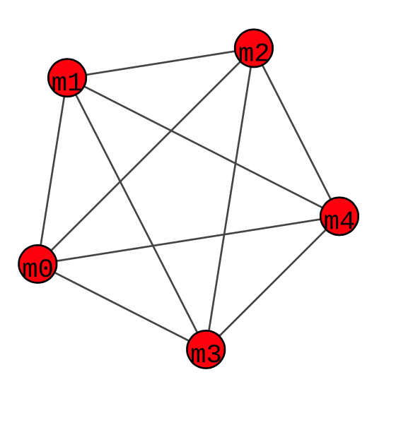
(a) The undirected graph with cycle.

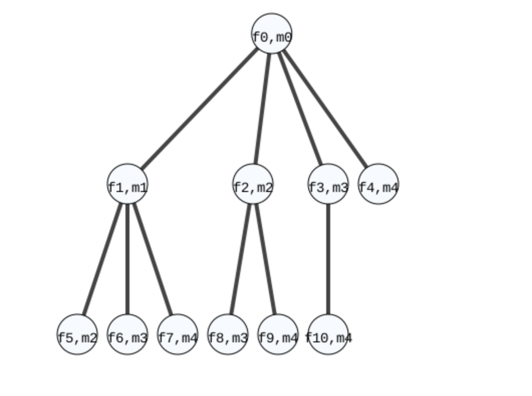
(b) The undirected tree after duplicating nodes.

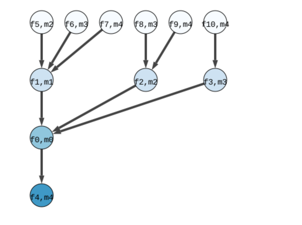
(c) A rooted tree representation of Fig. 6(a).

Figure 6: The pipeline to compute the Wasserstein barycenter via the MMOT approach. (a) is the corresponding undirected graph representation of the Gangbo-Świȩch type cost. (b) is the undirected graph representation after “unrolling” (a) by duplicating the nodes. (c) is the rooted tree representation after picking a root node and is updated by Algorithm 1.

First, the Wasserstein barycenter problem is represented as a MMOT with a complete undirected graph representation (see Figure 6(a)). Second, to solve MMOT under Gangbo-Świȩch type cost, we first unroll this undirected graph by duplicating nodes to remove cycles (see Figure 6(b)). We then use the method described in Section 4 to solve the unrolled problem, and obtain a dual solution that can be used to compute the barycenter.

Figure 7 demonstrates the use of this MMOT solution for shape interpolation. Inspired by an example in the POT (Python Optimal Transport) package [27], we use the four marginals “redcross”, “heart”, “tooth” and “duck” shown at the four corners of Figure 7. Each image is $1088\times 1088$ pixels.

All other plots in Figure 7 are a weighted Wasserstein barycenters computing using our MMOT approach. The weights correspond to bilinear interpolation between the corners. With comparable computational times to regularized solvers, our method provides much sharper interpolations.

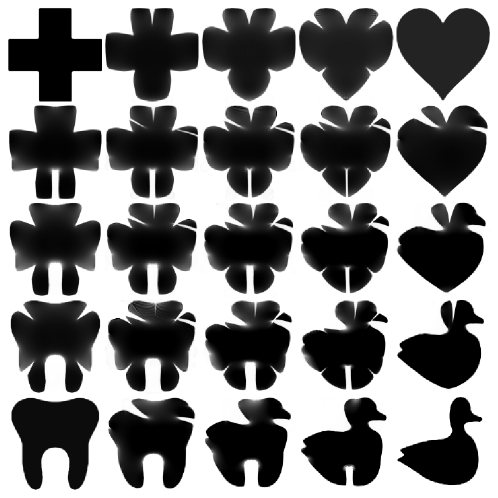
Figure 7: The Wasserstein barycenters of “redcross”, “heart”, “tooth” and “duck”. All interpolated images are obtained by solving (27) and computing (28). Those interpolated images show features from four marginals and have negligible diffusion effects.

6 Summary

We have presented a novel algorithm for multimarginal optimal transport problems with pairwise cost functions. Our solutions do not require regularizing the MMOT problem and are exact to within solver tolerance. To the best of our knowledge, this is the first extension of the back-and-forth method (BFM) introduced by [37] to the multi-marginal setting and the first approach capable of solving MMOT problems based on high resolution imagery. We leverage a graphical interpretation of the dual MMOT problem that can be applied to MMOT problems with an arbitrary number of marginals, as long as the cost function admits a pairwise representation.

As our method is inspired by BFM, our approach has the same gap between theoretical convergence analysis and numerical observations. Finding a convergence result under mild assumptions is therefore an interesting avenue for future work. It is worthy to note the hardness results in [2]. In the meanwhile, it is also natural to ask if these approaches can be generalized to cost functions which are not the sum of pairwise functions, for example the determinant type of cost function [15]. Note that one motivation for pairwise costs is the need for a fast $c$-transform. For pairwise cost function, the $c$-transform in high dimensions can be decomposed into nested 1D $c$-transforms, which can be obtained through fast algorithms of a divide-and-conquer type. As the $c$-transform is crucial to understand classical optimal transport theory, it maybe not be a coincidence that fast $c$-transforms are the key to numerical solutions.

Appendix A Supplement to Section 2.3

In this section, we provide with some comparisons between the $c$-transform and the well-known Legendre transform. The Legendre transform not only helps us to understand the $c$-transform, but also helps with our methods in at least two aspects: first, the closed form of optimal transport map for strictly convex function is in terms of the Legendre transform (see Theorem A.4); second, the $c$-transform is done via fast Legendre transform (see Lemma A.3), thanks to the code released in [bfm-github].

Definition A.1 (Subdifferential).

The subdifferential $\partial\phi(x)$ is defined as:

$$\partial\phi(x)\mathrel{\ensurestackMath{\stackon[1pt]{=}{\scriptscriptstyle\Delta}}}\left\{y\,\mid x^{\prime}\cdot y-\phi(x^{\prime})\mathrm{~{}is~{}maximal~{}at~{}}x^{\prime}=x\right\}.$$

Definition A.2 ($c$-superdifferential).

The $c$-superdifferential is defined as:

$$\partial^{c}f(x_{1})\mathrel{\ensurestackMath{\stackon[1pt]{=}{\scriptscriptstyle\Delta}}}\left\{x_{2}\,\mid c(x^{\prime},x_{2})-f(x^{\prime})\mathrm{~{}is~{}minimal~{}at~{}}x^{\prime}=x_{1}\right\}$$

Lemma A.3 and Theorem A.4 compare the Legendre transform with $c$-transform.

Lemma A.3 ([53, 4]).

For $X_{1}=X_{2}=\mathbb{R}^{d}$,

1. $\phi^{**}\leqslant\phi$, with equality if and only if $\phi$ is convex and lower semi-continuous;

2. $f^{cc}\geqslant f$, with equality if and only if $f$ is $c$-concave;

3. For $c(x_{1},x_{2})=\frac{1}{2}\mathinner{\!\left\lvert x_{1}-x_{2}\right\rvert}^{2}$, $f(x_{2})$ is $c$-concave if and only if $\phi(x_{2})=\frac{1}{2}\mathinner{\!\left\lvert x_{2}\right\rvert}^{2}-f(x_{2})$ is convex and lower semi-continuous. Moreover, $f^{c}(x_{1})=\frac{1}{2}\mathinner{\!\left\lvert x_{1}\right\rvert}^{2}-\phi^{*}(x_{1}).$

4. For convex function $\phi$ and $\phi^{*}$, we have

   $$y\in\partial\phi(x)\Longleftrightarrow\phi(x)+\phi^{*}(y)=x\cdot y\Longleftrightarrow x\in\partial\phi^{*}(y).$$

5. $x_{2}\in\partial^{c}f(x_{1})\Longleftrightarrow f(x_{1})+f^{c}(x_{2})=c(x_{1},x_{2})\Longleftrightarrow x_{1}\in\partial f^{c}(x_{2})$.

Theorem A.4 ([52, 30]).

1. Given a strictly convex and lower semi-continuous function $\phi(x)\mathrel{\mathop{\ordinarycolon}}\mathbb{R}^{d}\mapsto\mathbb{R}$, then

   $$y=\nabla\phi^{*}(x)$$

   is the unique maximizer to

   $$\sup_{y}\langle x,y\rangle-\phi(y).$$

2. Given $c(x_{1},x_{2})=h(x_{1}-x_{2})$ for some strictly convex function $h$, assume $g(x_{2})$ is a compactly supported continuous function, and $f(x_{1})=g^{c}(x_{1})$. If $f$ is differentiable at $x_{1}$, then

   $$x_{2}\mathrel{\ensurestackMath{\stackon[1pt]{=}{\scriptscriptstyle\Delta}}}x_{1}-(\nabla h)^{-1}(\nabla f(x_{1}))=x_{1}-\nabla h^{*}(\nabla f(x_{1}))$$

   is the unique minimizer to

   $$\inf_{x_{2}}c(x_{1},x_{2})-g(x_{2}).$$

   That is, $x_{2}$ is the unique pre-image of $x_{1}$ under the mapping $\partial^{c}g$.

Appendix B Supplementary Lemmas to Section 4.1

In this section, we provide with two supplementary lemmas. Lemma B.1 follows [30] to compute the Fréchet derivatives first, in order to define the gradient in $\dot{H}^{1}$. As the cost function gets more complex, finding the Fréchet derivatives through this way can be quite complex. Lemma B.3 serves as one motivation to our algorithm. It shows the difference roles the Kantorovich potentials play, from 2-marginal to multi-marginal. As a result, we are motivated by this to introduce the net potentials $f^{\prime}_{i}$ along the rooted tree.

Lemma B.1.

Let $X_{1},X_{2},X_{3}\subset\mathbb{R}^{d}$ be compact and convex domains and each measure $\mu_{i}\in\mathbb{P}(X_{i})$ has a strictly positive density, and $c(x_{1},x_{2},x_{3})=c_{12}(x_{1},x_{2})+c_{23}(x_{2},x_{3})$ where $c_{12}(x_{1},x_{2})=h_{1}(x_{1}-x_{2}),c_{23}(x_{2},x_{3})=h_{2}(x_{2}-x_{3})$ for some continuously differentiable and strictly convex functions $h_{1},h_{2}$. Define a functional

$$H((f_{2}+f_{3})^{c},f_{2},f_{3})=\int_{X_{1}}(f_{2}+f_{3})^{c}(x_{1})\mathrm{d}\mu_{1}+\int_{X_{2}}f_{2}(x_{2})\mathrm{d}\mu_{2}+\int_{X_{3}}f_{3}(x_{3})\mathrm{d}\mu_{3},$$

over the space of continuous function $f_{2}\mathrel{\mathop{\ordinarycolon}}X_{2}\mapsto\mathbb{R},f_{3}\mathrel{\mathop{\ordinarycolon}}X_{3}\mapsto\mathbb{R}$. Then

$$\delta_{f_{2}}H(f_{2};f_{3})=\mu_{2}-(S_{(f_{2}-f_{3}^{c_{23}})^{c_{12}}})_{\#}\mu_{1}.$$

Proof B.2.

The proof follows the proof to lemma 3 in [37]. Please refer to Proposition 2.9 in [30] for a detailed proof or refer to [31] for milder assumptions.

$$\lim_{\varepsilon\to 0}\dfrac{H((f_{2}+\varepsilon\xi+f_{3})^{c},f_{2}+\varepsilon\xi,f_{3})-H((f_{2}+f_{3})^{c},f_{2},f_{3})}{\varepsilon}$$

$$= \int_{X_{1}}\frac{(f_{2}(x_{2})+\varepsilon\xi(x_{2})+f_{3}(x_{3}))^{c}-(f_{2}(x_{2})+f_{3}(x_{3}))^{c}}{\varepsilon}\mathrm{d}\mu_{1}+\int_{X_{2}}\xi(x_{2})\mathrm{d}\mu_{2}$$

$$= \int_{X_{1}}\frac{(f_{2}-f_{3}^{c_{23}}+\varepsilon\xi)^{c_{12}}-(f_{2}-f_{3}^{c_{23}})^{c_{12}}}{\varepsilon}\mathrm{d}\mu_{1}+\int_{X_{2}}\xi(x_{2})\mathrm{d}\mu_{2}$$

$$= -\int_{X_{1}}\xi(S_{(f_{2}-f_{3}^{c_{23}})^{c_{12}}})(x_{1})\mathrm{d}\mu_{1}+\int_{X_{2}}\xi(x_{2})\mathrm{d}\mu_{2}$$

$$= -\int\xi\mathrm{d}[(S_{(f_{2}-f_{3}^{c_{23}})^{c_{12}}})_{\#}\mu_{1}+\int\xi\mathrm{d}\mu_{2}.$$

Lemma B.3.

Let $X_{1},X_{2},X_{3}\subset\mathbb{R}^{d}$ be compact and convex domains, and each measure $\mu_{i}\in\mathbb{P}(X_{i})$ is absolutely continuous with respect to the Lebesgue measure. For $c(x_{1},x_{2},x_{3})=c_{12}(x_{1},x_{2})+c_{23}(x_{2},x_{3})$, we have:

• If $(u_{1},v_{1}),(u_{2},v_{2})$ are optimal loading/unloading prices to the OT under cost $c_{12},c_{23}$ respectively, then $(f_{1},f_{2},f_{3})=(u_{1},v_{1}+u_{2},v_{2})$ is the Kantorovich potential to the MMOT under the cost $c(x_{1},x_{2},x_{3})$.

• If $(f_{1},f_{2},f_{3})$ is the Kantorovich potential to the MMOT under the cost $c$, then $(u_{1},v_{1})=(f_{1},f_{1}^{c_{12}}),(u_{2},v_{2})=(f_{2}-f_{1}^{c_{12}},f_{3})$ are optimal loading/unloading prices to the OT under cost $c_{12},c_{23}$ respectively.

Proof B.4.

Given $P\in\mathbb{P}(X_{1},X_{2},X_{3})$, we define $P_{1}(A)=\int_{A\times X_{2}\times X_{3}}\mathrm{d}P$ and $P_{1,2}(A\times B)=\int_{A\times B\times X_{3}}\mathrm{d}P$. On one hand

$$\inf_{P\in\Gamma(\mu_{1},\mu_{2},\mu_{3})}\int c_{12}(x_{1},x_{2})+c_{23}(x_{2},x_{3})\mathrm{d}P$$

$$= \inf_{P\in\Gamma(\mu_{1},\mu_{2},\mu_{3})}\int c_{12}(x_{1},x_{2})\mathrm{d}P_{1,2}+\int c_{23}(x_{2},x_{3})\mathrm{d}P_{2,3}$$

$$= \inf_{Q^{1}\in\Gamma(\mu_{1},\mu_{2})}\int c_{12}(x_{1},x_{2})\mathrm{d}Q^{1}+\inf_{Q^{2}\in\Gamma(\mu_{2},\mu_{3})}\int c_{23}(x_{2},x_{3})\mathrm{d}Q^{2}$$

(29) $$= \sup_{u_{1}+v_{1}\leqslant c_{12}}\int u_{1}\mathrm{d}\mu_{1}+\int v_{1}\mathrm{d}\mu_{2}+\sup_{u_{2}+v_{2}\leqslant c_{23}}\int u_{2}\mathrm{d}\mu_{2}+\int v_{2}\mathrm{d}\mu_{3};$$

On the other hand,

$$\inf_{P\in\Gamma(\mu_{1},\mu_{2},\mu_{3})}\int c_{12}(x_{1},x_{2})+c_{23}(x_{2},x_{3})\mathrm{d}P$$

(30) $$=\sup_{f_{1}+f_{2}+f_{3}\leqslant c}\int f_{1}\mathrm{d}\mu_{1}+\int f_{2}\mathrm{d}\mu_{2}+\int f_{3}\mathrm{d}\mu_{3}.$$

Given a tuple $(u_{1},v_{1},u_{2},v_{2})$ that achieves the maximum in (29), we define $f_{1}=u_{1},f_{2}=v_{1}+u_{2},f_{3}=v_{2}$, then

$$f_{1}(x_{1})+f_{2}(x_{2})+f_{3}(x_{3})=u_{1}(x_{1})+v_{1}(x_{2})+u_{2}(x_{2})+v_{2}(x_{3})\leqslant c_{12}(x_{1},x_{2})+c_{23}(x_{2},x_{3})$$

is an admissible solution to (30).

$$\eqref{eq:uvuv} =\int u_{1}\mathrm{d}\mu_{1}+\int(v_{1}+u_{2})\mathrm{d}\mu_{2}+\int v_{2}\mathrm{d}\mu_{3}$$

$$=\int f_{1}\mathrm{d}\mu_{1}+\int f_{2}\mathrm{d}\mu_{2}+\int f_{3}\mathrm{d}\mu_{3}$$

$$\leqslant\eqref{eq:f123}.$$

Since $\eqref{eq:uvuv}=\eqref{eq:f123}$, the tuple $(f_{1},f_{2},f_{3})$ is a maximizer to (30).

Given a tuple $(f_{1},f_{2},f_{3})$ that achieves the maximum in (30), we define $u_{1}=f_{1},v_{1}=f_{1}^{c_{12}},u_{2}=f_{2}-f_{1}^{c_{12}},v_{2}=f_{3}$.

We first show that $(u_{1},v_{1},v_{2},u_{3})$ is an admissible solution to (29). By definition, we just need to show that $u_{2}(x_{2})+v_{2}(x_{3})=f_{2}(x_{2})-f_{1}^{c_{12}}(x_{2})+f_{3}(x_{3})\leqslant c_{23}(x_{2},x_{3})$. By the duality theory, $f_{2}(x_{2})=(f_{1}+f_{3})^{c}=f_{1}^{c_{12}}(x_{2})+f_{3}^{c_{23}}(x_{2})$. Thus

$$f_{1}^{c_{12}}(x_{2})+f_{3}^{c_{23}}(x_{2})=f_{2}(x_{2})=v_{1}(x_{2})+u_{2}(x_{2})$$

$$\implies u_{2}(x_{2})=f_{3}^{c_{23}}(x_{2})$$

$$\implies u_{2}(x_{2})=v_{2}^{c_{23}}(x_{2}),$$

thus $u_{2}(x_{2})+v_{2}(x_{3})\leqslant c_{23}(x_{2},x_{3})$. As a result, $(u_{1},v_{1},v_{2},u_{3})$ is an admissible solution to (29). Analogously the above, it is the maximizer to (29) as well.

Appendix C Supplement to Section 5.3

Theorem C.1 ([1]).

For any $m$-tuple $(x_{1},\cdots,x_{m})\in(\mathbb{R}^{d})^{m}$ and weights $(\lambda_{1},\cdots,\lambda_{m})$ such that $\sum_{i=1}^{m}\lambda_{i}=1$, let us define the (Euclidean) barycenter map $T\mathrel{\mathop{\ordinarycolon}}(\mathbb{R}^{d})^{m}\mapsto\mathbb{R}^{d}$:

$$T(x_{1},\cdots,x_{m})=\sum_{i=1}^{m}\lambda_{i}x_{i}.$$

The optimal solution $P$ to the MMOT of Gangbo-Świȩch type cost

(31) $$\inf_{P\in\Gamma(\mu_{1},\cdots,\mu_{m})}\int_{(\mathbb{R}^{d})^{m}}\left(\sum_{1\leqslant i<j\leqslant m}\frac{\lambda_{i}\lambda_{j}}{2}\mathinner{\!\left\lvert x_{i}-x_{j}\right\rvert}^{2}\right)\mathrm{d}P(x_{1},\cdots,x_{m})$$

induces the barycenter $\mu$ to (27) by

$$\mu =(T)_{\#}P=(\sum_{j=1}^{m}\lambda_{j}T_{i}^{1})_{\#}\mu_{1};;$$

$$=(\mathop{}\mathopen{}\mathrm{id}-\frac{1}{\lambda_{i}}\nabla f_{i})_{\#}\mu_{i}.$$

where $(f_{i})$ are dual variables to (31), and for $x=(x_{1},\cdots,x_{m})$ $P$-almost everywhere,

$$x_{i}=T_{i}^{1}(x_{1})\mathrel{\ensurestackMath{\stackon[1pt]{=}{\scriptscriptstyle\Delta}}}\nabla\left(\frac{1}{2}\mathinner{\!\left\lvert\cdot\right\rvert}^{2}-\frac{f_{i}}{\lambda_{i}}\right)^{*}\circ\nabla\left(\frac{1}{2}\mathinner{\!\left\lvert\cdot\right\rvert}^{2}-\frac{f_{1}}{\lambda_{1}}\right)(x_{1}).$$

Proof C.2.

The proof is due to [32]. We follow the discussion in [1] but in terms of the dual variables $(f_{i})$, rather than the variables $g_{i}(x_{i})=\frac{\lambda_{i}(1-\lambda_{i})}{2}\mathinner{\!\left\lvert x_{i}\right\rvert}^{2}-f_{i}(x_{i})$ used in the convex analysis. More precisely, [1] consider the primal and dual problems:

(32a) $$\sup\int\left(\sum_{1\leqslant i<j\leqslant m}\lambda_{i}\lambda_{j}x_{i}x_{j}\right)\mathrm{d}P;$$

(32b) $$\inf\sum_{i=1}^{m}\int g_{i}\mathrm{d}\mu_{i}\qquad\textrm{~{}subject to~{}}\sum_{i=1}^{m}g_{i}\geqslant\sum_{1\leqslant i<j\leqslant m}\lambda_{i}\lambda_{j}x_{i}x_{j}.$$

We considered the following instead:

(33a) $$\inf\int\sum_{1\leqslant i<j\leqslant m}\frac{\lambda_{i}\lambda_{j}}{2}\mathinner{\!\left\lvert x_{i}-x_{j}\right\rvert}^{2}\mathrm{d}P;$$

(33b) $$\sup\sum_{i=1}^{m}\int f_{i}\mathrm{d}\mu_{i}\qquad\textrm{~{}subject to~{}}\sum_{i=1}^{m}f_{i}\leqslant\sum_{1\leqslant i<j\leqslant m}\frac{\lambda_{i}\lambda_{j}}{2}\mathinner{\!\left\lvert x_{i}-x_{j}\right\rvert}^{2}.$$

These two sets of problems are equivalent under the change of variables:

$$g_{i}(x_{i})=\frac{\lambda_{i}(1-\lambda_{i})}{2}\mathinner{\!\left\lvert x_{i}\right\rvert}^{2}-f_{i}(x_{i}).$$

The optimal condition to (32) is for $P$-a.e. $x=(x_{1},\cdots,x_{m})$

$$\nabla g_{i}(x_{i})=\lambda_{i}\sum_{j\neq i}\lambda_{j}x_{j}$$

$$\Longleftrightarrow \nabla\left(\frac{\lambda_{i}}{2}\mathinner{\!\left\lvert\cdot\right\rvert}^{2}+\frac{g_{i}}{\lambda_{i}}\right)(x_{i})=\sum_{j=1}^{m}\lambda_{j}x_{j}=\nabla\left(\frac{\lambda_{1}}{2}\mathinner{\!\left\lvert\cdot\right\rvert}^{2}+\frac{g_{1}}{\lambda_{1}}\right)(x_{1})$$

$$\Longleftrightarrow x_{i}=\nabla\left(\frac{\lambda_{i}}{2}\mathinner{\!\left\lvert\cdot\right\rvert}^{2}+\frac{g_{i}}{\lambda_{i}}\right)^{*}\circ\nabla\left(\frac{\lambda_{1}}{2}\mathinner{\!\left\lvert\cdot\right\rvert}^{2}+\frac{g_{1}}{\lambda_{1}}\right)(x_{1})\mathrel{\ensurestackMath{\stackon[1pt]{=}{\scriptscriptstyle\Delta}}}T_{i}^{1}(x_{1}).$$

By the change of variables, the optimal condition to (33) is for $P$-a.e. $x=(x_{1},\cdots,x_{m})$

$$\nabla f_{i}(x_{i})=\lambda_{i}(1-\lambda_{i})x_{i}-\lambda_{i}\sum_{j\neq i}\lambda_{j}x_{j}=\lambda_{i}(x_{i}-\sum_{j}\lambda_{j}x_{j})$$

$$\Longleftrightarrow \nabla\left(\frac{1}{2}\mathinner{\!\left\lvert\cdot\right\rvert}^{2}-\frac{f_{i}}{\lambda_{i}}\right)(x_{i})=\sum_{j}\lambda_{j}x_{j}=\nabla\left(\frac{1}{2}\mathinner{\!\left\lvert\cdot\right\rvert}^{2}-\frac{f_{1}}{\lambda_{1}}\right)(x_{1})$$

$$\Longleftrightarrow x_{i}=\nabla\left(\frac{1}{2}\mathinner{\!\left\lvert\cdot\right\rvert}^{2}-\frac{f_{i}}{\lambda_{i}}\right)^{*}\circ\nabla\left(\frac{1}{2}\mathinner{\!\left\lvert\cdot\right\rvert}^{2}-\frac{f_{1}}{\lambda_{1}}\right)(x_{1})=T_{i}^{1}(x_{1}).$$

References

• [1] M. Agueh and G. Carlier, Barycenters in the Wasserstein space, SIAM J. Math. Anal., 43 (2011), pp. 904–924, https://doi.org/10.1137/100805741.
• [2] J. Altschuler and E. Boix-Adserà, Hardness results for multimarginal optimal transport problems, Discrete Optimization, 42 (2021), p. 100669, https://doi.org/https://doi.org/10.1016/j.disopt.2021.100669.
• [3] J. Altschuler and E. Boix-Adserà, Polynomial-time algorithms for multimarginal optimal transport problems with structure, Math. Program., (2022), https://doi.org/10.1007/s10107-022-01868-7.
• [4] L. Ambrosio, E. Brué, and D. Semola, Lectures on optimal transport, vol. 130 of Unitext, Springer, Cham, 2021, https://doi.org/10.1007/978-3-030-72162-6. La Matematica per il 3+2.
• [5] L. Ambrosio and N. Gigli, A user’s guide to optimal transport, in Modelling and optimisation of flows on networks, vol. 2062 of Lecture Notes in Math., Springer, 2013, pp. 1–155, https://doi.org/10.1007/978-3-642-32160-3_1.
• [6] L. Ambrosio, N. Gigli, and G. Savaré, Gradient flows in metric spaces and in the space of probability measures, Lectures in Mathematics ETH Zürich, Birkhäuser Verlag, Basel, second ed., 2008.
• [7] M. Arjovsky, S. Chintala, and L. Bottou, Wasserstein generative adversarial networks, in International conference on machine learning, PMLR, 2017, pp. 214–223.
• [8] J. Benamou and Y. Brenier, A computational fluid mechanics solution to the Monge-Kantorovich mass transfer problem, Numer. Math., 84 (2000), pp. 375–393, https://doi.org/10.1007/s002110050002.
• [9] J. Benamou, G. Carlier, M. Cuturi, L. Nenna, and G. Peyré, Iterative Bregman projections for regularized transportation problems, SIAM J. Sci. Comput., 37 (2015), pp. A1111–A1138, https://doi.org/10.1137/141000439.
• [10] J. Benamou, B. D. Froese, and A. M. Oberman, Numerical solution of the optimal transportation problem using the Monge-Ampère equation, J. Comput. Phys., 260 (2014), pp. 107–126, https://doi.org/10.1016/j.jcp.2013.12.015.
• [11] M. Bernot, V. Caselles, and J.-M. Morel, The structure of branched transportation networks, Calc. Var. Partial Differential Equations, 32 (2008), pp. 279–317, https://doi.org/10.1007/s00526-007-0139-0.
• [12] Y. Brenier, The least action principle and the related concept of generalized flows for incompressible perfect fluids, J. Amer. Math. Soc., 2 (1989), pp. 225–255, https://doi.org/10.2307/1990977.
• [13] Y. Brenier, Polar factorization and monotone rearrangement of vector-valued functions, Comm. Pure Appl. Math., 44 (1991), pp. 375–417, https://doi.org/10.1002/cpa.3160440402.
• [14] Y. Brenier, Generalized solutions and hydrostatic approximation of the Euler equations, Physica D: Nonlinear Phenomena, 237 (2008), pp. 1982–1988.
• [15] G. Carlier and B. Nazaret, Optimal transportation for the determinant, ESAIM Control Optim. Calc. Var., 14 (2008), pp. 678–698, https://doi.org/10.1051/cocv:2008006.
• [16] M. Caron, I. Misra, J. Mairal, P. Goyal, P. Bojanowski, and A. Joulin, Unsupervised learning of visual features by contrasting cluster assignments, in Advances in Neural Information Processing Systems, vol. 33, 2020, pp. 9912–9924.
• [17] N. Courty, R. Flamary, A. Habrard, and A. Rakotomamonjy, Joint distribution optimal transportation for domain adaptation, Advances in Neural Information Processing Systems, 30 (2017).
• [18] M. Cuturi, Sinkhorn distances: Lightspeed computation of optimal transport, Advances in neural information processing systems, 26 (2013).
• [19] M. Cuturi and G. Peyré, Semidual regularized optimal transport, SIAM Rev., 60 (2018), pp. 941–965, https://doi.org/10.1137/18M1208654.
• [20] S. De, A. P. Bartók, G. Csányi, and M. Ceriotti, Comparing molecules and solids across structural and alchemical space, Physical Chemistry Chemical Physics, 18 (2016), pp. 13754–13769, https://doi.org/10.1039/C6CP00415F.
• [21] A. de Acosta, Invariance principles in probability for triangular arrays of $B$-valued random vectors and some applications, Ann. Probab., 10 (1982), pp. 346–373, http://links.jstor.org/sici?sici=0091-1798(198205)10:2<346:IPIPFT>2.0.CO;2-8&origin=MSN.
• [22] A. Dessein, N. Papadakis, and J.-L. Rouas, Regularized optimal transport and the rot mover’s distance, The Journal of Machine Learning Research, 19 (2018), pp. 590–642.
• [23] S. Di Marino, A. Gerolin, and L. Nenna, Optimal transportation theory with repulsive costs, in Topological optimization and optimal transport, vol. 17 of Radon Ser. Comput. Appl. Math., De Gruyter, Berlin, 2017, pp. 204–256.
• [24] F. Elvander, I. Haasler, A. Jakobsson, and J. Karlsson, Multi-marginal optimal transport using partial information with applications in robust localization and sensor fusion, Signal Processing, 171 (2020), p. 107474.
• [25] J. Fan, I. Haasler, J. Karlsson, and Y. Chen, On the complexity of the optimal transport problem with graph-structured cost, in Proceedings of The 25th International Conference on Artificial Intelligence and Statistics, PMLR, 2022, pp. 9147–9165, https://proceedings.mlr.press/v151/fan22a.html.
• [26] J. Feydy, T. Séjourné, F.-X. Vialard, S. Amari, A. Trouvé, and G. Peyré, Interpolating between optimal transport and MMD using Sinkhorn divergences, in The 22nd International Conference on Artificial Intelligence and Statistics, PMLR, 2019, pp. 2681–2690.
• [27] R. Flamary, N. Courty, A. Gramfort, M. Z. Alaya, A. Boisbunon, S. Chambon, L. Chapel, A. Corenflos, K. Fatras, N. Fournier, L. Gautheron, N. Gayraud, H. Janati, A. Rakotomamonjy, I. Redko, A. Rolet, A. Schutz, V. Seguy, D. J. Sutherland, R. Tavenard, A. Tong, and T. Vayer, POT: Python Optimal Transport, Journal of Machine Learning Research, 22 (2021), pp. 1–8, http://jmlr.org/papers/v22/20-451.html.
• [28] G. Friesecke, A. S. Schulz, and D. Vögler, Genetic column generation: fast computation of high-dimensional multimarginal optimal transport problems, SIAM J. Sci. Comput., 44 (2022), pp. A1632–A1654, https://doi.org/10.1137/21M140732X, https://doi.org/10.1137/21M140732X.
• [29] C. Frogner, C. Zhang, H. Mobahi, M. Araya, and T. A. Poggio, Learning with a Wasserstein loss, in Advances in neural information processing systems, vol. 28, 2015, https://proceedings.neurips.cc/paper/2015/file/a9eb812238f753132652ae09963a05e9-Paper.pdf.
• [30] W. Gangbo, An introduction to the mass transportation theory and its applications. UCLA lecture notes, 2004, https://www.math.ucla.edu/~wgangbo/publications/notecmu.pdf.
• [31] W. Gangbo and R. J. McCann, The geometry of optimal transportation, Acta Math., 177 (1996), pp. 113–161, https://doi.org/10.1007/BF02392620.
• [32] W. Gangbo and A. Świȩch, Optimal maps for the multidimensional Monge-Kantorovich problem, Comm. Pure Appl. Math., 51 (1998), pp. 23–45, https://doi.org/10.1002/(SICI)1097-0312(199801)51:1<23::AID-CPA2>3.0.CO;2-H.
• [33] N. Garcia Trillos, M. Jacobs, and J. Kim, The multimarginal optimal transport formulation of adversarial multiclass classification, arXiv:2204.12676, (2022).
• [34] A. Genevay, G. Peyré, and M. Cuturi, Learning generative models with Sinkhorn divergences, in International Conference on Artificial Intelligence and Statistics, PMLR, 2018, pp. 1608–1617.
• [35] I. Haasler, A. Ringh, Y. Chen, and J. Karlsson, Multimarginal optimal transport with a tree-structured cost and the Schrödinger bridge problem, SIAM J. Control Optim., 59 (2021), pp. 2428–2453, https://doi.org/10.1137/20M1320195.
• [36] I. Haasler, R. Singh, Q. Zhang, J. Karlsson, and Y. Chen, Multi-marginal optimal transport and probabilistic graphical models, IEEE Trans. Inform. Theory, 67 (2021), pp. 4647–4668, https://doi.org/10.1109/tit.2021.3077465.
• [37] M. Jacobs and F. Léger, A fast approach to optimal transport: the back-and-forth method, Numer. Math., 146 (2020), pp. 513–544, https://doi.org/10.1007/s00211-020-01154-8.
• [38] M. Jacobs and F. Léger, The back-and-forth method. https://github.com/Math-Jacobs/bfm, 2021.
• [39] H. G. Kellerer, Duality theorems for marginal problems, Z. Wahrsch. Verw. Gebiete, 67 (1984), pp. 399–432, https://doi.org/10.1007/BF00532047.
• [40] Y. Khoo, L. Lin, M. Lindsey, and L. Ying, Semidefinite relaxation of multimarginal optimal transport for strictly correlated electrons in second quantization, SIAM J. Sci. Comput., 42 (2020), pp. B1462–B1489, https://doi.org/10.1137/20M1310977, https://doi.org/10.1137/20M1310977.
• [41] J. Kitagawa, Q. Mérigot, and B. Thibert, Convergence of a Newton algorithm for semi-discrete optimal transport, J. Eur. Math. Soc. (JEMS), 21 (2019), pp. 2603–2651, https://doi.org/10.4171/JEMS/889.
• [42] T. Lin, N. Ho, M. Cuturi, and M. I. Jordan, On the complexity of approximating multimarginal optimal transport, Journal of Machine Learning Research, 23 (2022), pp. 1–43, http://jmlr.org/papers/v23/19-843.html.
• [43] Y. Lucet, Faster than the fast Legendre transform, the linear-time Legendre transform, Numerical Algorithms, 16 (1997), pp. 171–185.
• [44] F. Maddalena, S. Solimini, and J. Morel, A variational model of irrigation patterns, Interfaces Free Bound., 5 (2003), pp. 391–415, https://doi.org/10.4171/IFB/85.
• [45] Q. Mérigot and J. Mirebeau, Minimal geodesics along volume-preserving maps, through semidiscrete optimal transport, SIAM J. Numer. Anal., 54 (2016), pp. 3465–3492, https://doi.org/10.1137/15M1017235.
• [46] A. Neufeld and Q. Xiang, Numerical method for feasible and approximately optimal solutions of multi-marginal optimal transport beyond discrete measures, arXiv:2203.01633, (2022).
• [47] M. Parno and B. Zhou, MMOT2d. https://github.com/simda-muri/mmot, 2022.
• [48] M. D. Parno, B. A. West, A. J. Song, T. S. Hodgdon, and D. T. O’Connor, Remote measurement of sea ice dynamics with regularized optimal transport, Geophysical Research Letters, 46 (2019), pp. 5341–5350, https://doi.org/10.1029/2019GL083037.
• [49] B. Pass, Uniqueness and Monge solutions in the multimarginal optimal transportation problem, SIAM J. Math. Anal., 43 (2011), pp. 2758–2775, https://doi.org/10.1137/100804917.
• [50] B. Pass, Multi-marginal optimal transport: theory and applications, ESAIM Math. Model. Numer. Anal., 49 (2015), pp. 1771–1790, https://doi.org/10.1051/m2an/2015020.
• [51] M. Peletier and M. Röger, Partial localization, lipid bilayers, and the elastica functional, Arch. Ration. Mech. Anal., 193 (2009), pp. 475–537, https://doi.org/10.1007/s00205-008-0150-4.
• [52] R. T. Rockafellar, Convex analysis, Princeton Mathematical Series, No. 28, Princeton University Press, Princeton, N.J., 1970.
• [53] F. Santambrogio, Optimal transport for applied mathematicians, vol. 87 of Progress in Nonlinear Differential Equations and their Applications, Birkhäuser, 2015, https://doi.org/10.1007/978-3-319-20828-2. Calculus of variations, PDEs, and modeling.
• [54] L. Saumier, B. Khouider, and M. Agueh, Optimal transport for particle image velocimetry: real data and postprocessing algorithms, SIAM J. Appl. Math., 75 (2015), pp. 2495–2514, https://doi.org/10.1137/140988814.
• [55] B. Schmitzer, Stabilized sparse scaling algorithms for entropy regularized transport problems, SIAM J. Sci. Comput., 41 (2019), pp. A1443–A1481, https://doi.org/10.1137/16M1106018.
• [56] R. Sinkhorn and P. Knopp, Concerning nonnegative matrices and doubly stochastic matrices, Pacific J. Math., 21 (1967), pp. 343–348, http://projecteuclid.org/euclid.pjm/1102992505.
• [57] J. Solomon, F. De Goes, G. Peyré, M. Cuturi, A. Butscher, A. Nguyen, T. Du, and L. Guibas, Convolutional Wasserstein distances: efficient optimal transportation on geometric domains, ACM Transactions on Graphics (ToG), 34 (2015), pp. 1–11, https://doi.org/10.1145/2766963.
• [58] C. Villani, Topics in optimal transportation, vol. 58 of Graduate Studies in Mathematics, American Mathematical Society, Providence, RI, 2003, https://doi.org/10.1090/gsm/058.
• [59] Q. Xia, Optimal paths related to transport problems, Commun. Contemp. Math., 5 (2003), pp. 251–279, https://doi.org/10.1142/S021919970300094X.
• [60] Q. Xia and B. Zhou, The existence of minimizers for an isoperimetric problem with Wasserstein penalty term in unbounded domains, Advances in Calculus of Variations, (2021), https://doi.org/10.1515/acv-2020-0083.
• [61] Y. Yang, B. Engquist, J. Sun, and B. F. Hamfeldt, Application of optimal transport and the quadratic Wasserstein metric to full-waveform inversion, Geophysics, 83 (2018), pp. R43–R62, https://doi.org/10.1190/geo2016-0663.1.