Modified Generalized-Brillouin-Zone Theory with On-site Disorders

Abstract

We study the characterization of the non-Hermitian skin effect (NHSE) in non-Hermitian systems with on-site disorder. We extend the application of generalized-Brillouin-zone (GBZ) theory to these systems. By proposing a modified GBZ theory, we give a faithfully description of the NHSE. For applications, we obtain a unified $\beta$ for system with long-range hopping, and explain the conventional-GBZ irrelevance of the magnetic suppression of the NHSE in the previous study.

I Introduction

Systems described by non-Hermitian Hamiltonians have been attracting intensive attention in recent years NH1 ; NH2 ; NH3 ; NH4 ; NH5 ; NH6 ; NH7 ; NH8 ; NH9 ; TI1 ; TI2 ; TI3 ; TI4 ; TI5 ; TI6 ; TI7 ; TI8 ; TI9 ; TI10 ; TI11 ; TI12 ; TI13 ; TI14 ; TI15 ; TI16 ; Dis1 ; Dis2 ; Dis3 ; Dis4 ; Dis5 ; Dis6 ; Dis7 ; Dis8 ; Dis9 ; Dis10 ; Dis11 ; Mag1 ; Mag2 ; E ; EP1 ; EP2 ; EP3 ; EP4 ; EP5 ; EP6 ; EP7 ; EP8 ; EP9 ; EP10 ; EP11 ; EP12 ; EP13 ; PG ; QM ; NHSE1 ; NHSE2 ; NHSE3 ; NHSE4 ; NHSE5 ; NHSE6 ; NHSE7 ; NHSE8 ; NHSE9 ; NHSE10 ; NHSE11 ; NHSE12 ; NHSE13 ; NHSE14 ; NHSE15 ; NHSE16 ; NHSE17 ; NHSE18 ; NHSE19 ; NHSE20 ; NHSE21 ; NHSE22 ; NHSE23 ; NHSE24 ; NHSE25 ; NHSE26 ; NHSE27 . A large number of interesting phenomena are reported EP1 ; EP2 ; EP3 ; EP4 ; EP5 ; EP6 ; EP7 ; EP8 ; EP9 ; EP10 ; EP11 ; EP12 ; EP13 ; PG ; QM ; NHSE1 ; NHSE2 ; NHSE3 ; NHSE4 ; NHSE5 ; NHSE6 ; NHSE7 ; NHSE8 ; NHSE9 ; NHSE10 ; NHSE11 ; NHSE12 ; NHSE13 ; NHSE14 ; NHSE15 ; NHSE16 ; NHSE17 ; NHSE18 ; NHSE19 ; NHSE20 ; NHSE21 ; NHSE22 ; NHSE23 ; NHSE24 ; NHSE25 ; NHSE26 , among which the non-Hermitian skin effect (NHSE) NHSE1 ; NHSE2 ; NHSE3 ; NHSE4 ; NHSE5 ; NHSE6 ; NHSE7 ; NHSE8 ; NHSE9 ; NHSE10 ; NHSE11 ; NHSE12 ; NHSE13 ; NHSE14 ; NHSE15 ; NHSE16 ; NHSE17 ; NHSE18 ; NHSE19 ; NHSE20 ; NHSE21 ; NHSE22 ; NHSE23 ; NHSE24 ; NHSE25 ; NHSE26 ; NHSE27 has been the focus. The existence of the NHSE indicates that the conventional bulk-boundary correspondence fails NHSE1 ; NHSE2 ; NHSE3 ; NHSE4 ; NHSE5 . Meanwhile, the bulk spectrum shows distinct features for the open boundary (OBC) and periodic boundary (PBC) conditions, showing the collapse of the bulk-bulk correspondence (BBC). In order to accomplish the BBC, the generalized-Brillouin-zone (GBZ) theory NHSE2 ; NHSE3 ; NHSE4 introduces a similarity transform for the Hamiltonian, which eliminates the NHSE.

Nevertheless, a recent study Mag1 showed that the conventional GBZ theory fails to capture the NHSE’s features for samples under a magnetic field where the BBC still holds. Loosely speaking, such a model can be considered as the one-dimensional model with an on-site disorder QusiC . Very recently, the modified GBZ theory for the disordered samples was reported Dis11 , which breaks the limitation of the translational invariance required by the conventional GBZ theory. The essence of the modified GBZ theory is to search the minimum of a polynomial $\mathcal{F}(E,\beta)=|\det[E-\mathcal{H_{PBC}}(\beta)]-\det[E-\mathcal{H_{OBC}}]|$. However, applying the modified GBZ theory for samples with the on-site disorder is still unreported, which leaves the GBZ irrelevance of magnetic suppression of NHSE unexplained. Thus, there is an urgent need to study the influences of on-site disorder on the GBZ theory.

In this paper, we give the faithful characterization of the NHSE for samples with on-site disorders based on the modified GBZ theory. We uncover that the transformation coefficient $\beta=\beta_{min}$ determined by the minimum of the polynomial $\mathcal{F}(E,\beta)$ gives an interval instead of a single point. To unify the description of NHSEs, we demonstrate that the modified GBZ theory also requires the minimization of $|\beta_{min}-1|$. Based on these considerations, we clarify the applicability of the GBZ theory in several prototypical disordered non-Hermitian models. In details, a unified transformation coefficient $\beta_{min}$ to achieve the global BBC for disordered samples with long-range hopping is obtained. A faithful description of NHSEs for samples under the magnetic field is also clarified. Our work removes the ambiguity of the understanding of GBZ theory in the previous studies.

II model and method

We start from the disordered Hatano-Nelson modelHN with Hamiltonian:

$$\mathcal{H}=\sum_{i}\varepsilon_{i}c^{\dagger}_{i}c_{i}+t^{+}c^{\dagger}_{i}c_{i+1}+t^{-}c^{\dagger}_{i+1}c_{i},$$ (1)

where $c^{\dagger}_{i}$ ($c_{i}$) is the creation (annihilation) opperator on the site $i$. $t^{\pm}=(t\pm\gamma)$ represents the nearest-neighbor hopping and $\gamma$ encodes the non-Hermitian strength. We fix $t=1$. $\varepsilon_{i}\in[-W/2,W/2]$ denotes the on-site disorder Anderson with $W$ the disorder strength. The Hamiltonian under OBC and PBC are marked as $\mathcal{H_{OBC}}$ and $\mathcal{H_{PBC}}$, respectively.

Following the modified GBZ theory Dis11 , we adopt the transformation $t^{\pm}\rightarrow t^{\pm}\beta^{\pm 1}$. $\beta$ is the transformation coefficient, which gives a quantitative description of NHSE Dis11 ; NHSE3 ; NHSE4 . The transformed Hamiltonian under PBC [$\mathcal{H_{GBZ}}\equiv\mathcal{H_{PBC}}(\beta)$] satisfies Dis11 :

$$\begin{split}\det[E-\mathcal{H}_{\mathcal{GBZ};N\times N}]=\det[E-\mathcal{H}_{\mathcal{OBC};N\times N}]+f_{\mathcal{PBC}},\end{split}$$ (2)

where $f_{\mathcal{PBC}}=t^{+}t^{-}\det[E-\mathcal{H}_{\mathcal{OBC};N-2\times N-2}]+(t^{+})^{N}\beta^{N}+(t^{-})^{N}\beta^{-N}$. $N$ denotes the size of the Hamiltonian and $E$ is the eigenvalue of $\mathcal{H}_{\mathcal{OBC};N\times N}$. We mark $\mathcal{F}(E,\beta)=|\det[E-\mathcal{H_{PBC}}(\beta)]-\det[E-\mathcal{H_{OBC}}]|$ as follow:

$$\begin{split}\mathcal{F}(E,\beta)&\equiv|f_{\mathcal{PBC}}|=|\mathcal{F}_{1}+\mathcal{F}_{2}|,\end{split}$$ (3)

where $\mathcal{F}_{1}=t^{+}t^{-}\det[E-\mathcal{H}_{\mathcal{OBC};N-2\times N-2}]$ and $\mathcal{F}_{2}=(t^{+})^{N}\beta^{N}+(t^{-})^{N}\beta^{-N}$. For $W=0$, one should notice $\mathcal{F}_{1}$ is negligible since $\det[E-\mathcal{H}_{\mathcal{OBC};N\times N}]=0$ and $\det[E-\mathcal{H}_{\mathcal{OBC};N-2\times N-2}]\approx 0$ Dis11 . The modified GBZ theory requires the minimum of $\mathcal{F}(E,\beta)=|\mathcal{F}_{2}|$, which gives rise to $\beta_{min}=\sqrt{|t^{-}/t^{+}|}$, consistent with the previous GBZ theory NHSE3 ; NHSE4 . Here, $\beta=\beta_{min}$ gives the minimum of the polynomial $\mathcal{F}(E,\beta)$.

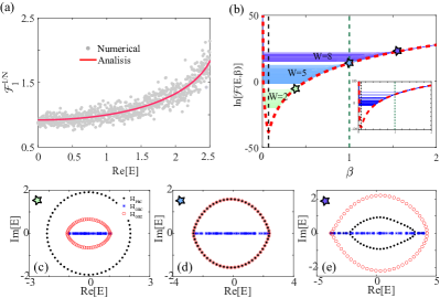
Figure 1: (a) The analytical (red line) and numerical (gray dots) results of $\mathcal{F}^{1/N}_{1}$ versus the eigenvalue $E$ for $W=5$. (b) $\ln[\mathcal{F}(E,\beta)]$ versus $\beta$ for different eigenvalues with $E\in[-W/2,W/2]$ under disorder strengths: $W=2$ (green), $W=5$ (blue) and $W=8$ (purple). Pentagrams mark the right boundary of the plateaus for $E=\frac{W}{2}$. The red dashed line is the plot of $\ln[|\mathcal{F}_{2}|]$ for clean samples. Inset is the numerical results for $\mathcal{F}(E,\beta)=|\det[E-\mathcal{H_{PBC}}(\beta)]-\det[E-\mathcal{H_{OBC}}]|$ with $W=8$. (c)-(e) The real part $Re[E]$ versus the imaginary part $Im[E]$ of the eigenvalues $E$ for (c) $W=2$; (d) $W=5$; (e) $W=8$. $\beta$ for $\mathcal{H_{GBZ}}$ is marked in (b). Other parameters are set as $\gamma=0.99$ and $N=60$.

In the following, we apply the modified GBZ theory for samples with on-site disorders. When disorder is strong enough, we demonstrate that $\mathcal{F}_{1}$ has considerable influence on achieving the appropriate characterization of the NHSE since $[\mathcal{F}_{1}(E)]/min[|\mathcal{F}_{2}(\beta)|]\propto(E-\varepsilon_{i})/t$. We have to emphasize that $\mathcal{F}_{1}$ can be neglected for samples with hopping disorder in our previous study Dis11 , since the NHSEs are mostly contributed from eigenstates near $E=0$ for considerable disorder. Noticing $[\mathcal{F}_{1}(E)]/min[|\mathcal{F}_{2}(\beta)|]\propto E/t\sim 0$, it is reasonable to neglect $\mathcal{F}_{1}$ in our previous study Dis11 . Besides, for weak disorder, $\mathcal{F}_{1}$ is always negligible.

For illustration purpose, we first consider $t\sim\gamma$, where the Hamiltonian $\mathcal{H}_{OBC;n\times n}$ is roughly a triangular matrix. The eigenvalue of $\mathcal{H}_{\mathcal{OBC};n\times n}$ can be considered to satisfy $E_{\mathcal{OBC};n}\in\left\{E_{i}\right\}\approx\left\{\varepsilon_{1},\varepsilon_{2},\ldots,\varepsilon_{i},\ldots,\varepsilon_{n}\right\}$ with $E_{\mathcal{OBC};n}\in[-W/2,W/2]$. For $|W/2|>|t^{\pm}|$ and thermaldynamic limit $N\rightarrow\infty$, $\mathcal{F}_{1}=t^{+}t^{-}\det[E-\mathcal{H}_{\mathcal{OBC};N-2\times N-2}]$ can be rewritten as

$$\begin{split}\mathcal{F}_{1}\approx\prod_{i=1}^{N-2}(E-E_{i})t^{+}t^{-}\approx\prod_{i=1}^{N}(E-E_{i}).\end{split}$$ (4)

$E_{i}\in E_{\mathcal{OBC};N-2}$ is the eigenvalue of $\mathcal{H}_{\mathcal{OBC};N-2\times N-2}$. By considering the differences of the eigenvalues between $\mathcal{H}_{\mathcal{OBC};N\times N}$ and $\mathcal{H}_{\mathcal{OBC};N-2\times N-2}$, the analytical formula of $\mathcal{F}_{1}$ is obtained [see the Appendix for more details]:

$$\begin{split}\mathcal{F}_{1}=[(E-\frac{W}{2})^{(\frac{1}{2}-\frac{E}{W})}(E+\frac{W}{2})^{(\frac{1}{2}+\frac{E}{W})}e^{-1}]^{N}.\end{split}$$ (5)

As plotted in Fig. 1(a), $\mathcal{F}_{1}\sim 2^{N}$ for $E=\frac{W}{2}$, which is comparable with $\mathcal{F}_{2}$. Thus, $\mathcal{F}_{1}$ should have distinct influences and cannot be neglected.

In order to better understand the influence of $\mathcal{F}_{1}$, we plot $\mathcal{F}(E,\beta)$ versus $\beta$ based on our analytical results, shown in Fig. 1(b). By neglecting $\mathcal{F}_{1}$ in Eq. (3), the minimum of $\mathcal{F}(E,\beta)=|\mathcal{F}_{2}|=|(t^{+})^{N}\beta^{N}+(t^{-})^{N}\beta^{-N}|$ and $\beta_{min}$ are $W$ and $E$ independent. After considering $\mathcal{F}_{1}$, the global minimum of $\mathcal{F}(E,\beta)=|\mathcal{F}_{1}+\mathcal{F}_{2}|$ is still $\beta_{min}=\sqrt{|t^{-}/t^{+}|}$. Nevertheless, $\mathcal{F}(E,\beta)$ versus $\beta$ give rise to some plateaus, which is distinct from the result for clean samples [red dashed line in Fig. 1(b)]. Moreover, the value of the plateau roughly equals to the global minimum $\mathcal{F}(E,\sqrt{|t^{-}/t^{+}|})$. Such a feature is also identified by numerical calculations directly based on Eq. (3), as shown in the inset of Fig. 1(b). Due to the existence of the plateau for $\mathcal{F}(E,\beta)$, the $\beta_{min}$ should be extended from a single point $\beta_{min}=\sqrt{|t^{-}/t^{+}|}$ to an interval $\beta_{min}\in[\Delta^{-},\Delta^{+}]$ for a specific eigenvalue $E$. Here, $\Delta^{\pm}$ is determined at the boundary of the plateau.

Since $\beta_{min}\in[\Delta^{-},\Delta^{+}]$ roughly give the same value $\mathcal{F}(E,\beta_{min})$, all the $\beta_{min}$ in the interval can be adopted to realize the BBC with considerable accuracy, and every $\beta_{min}$ gives a correct description of NHSEs. Nevertheless, to compare the NHSEs for different cases, we demonstrate that the best choices of $\beta_{min}$ should satisfy two key points: (1) it should be in the range $\beta_{min}\in[\Delta^{-},\Delta^{+}]$, which captures a correct description of NHSEs; (2) $\beta_{min}$ is the one closest to $\beta=1$, i.e., $|\beta_{min}-1|$ has the minimum value.

Physically, the criterion of BBC ensures Dis11 ; NHSE3 :

$$\left\{\begin{array}[]{l}\mathcal{H_{OBC}}\psi_{n}=E_{n}\psi_{n};\\ \mathcal{H_{PBC}}(\beta_{min})\widetilde{\psi}_{n}(\beta_{min})=E_{n}\widetilde{\psi}_{n}(\beta_{min});\\ \psi_{n}\approx S\widetilde{\psi}_{n}(\beta_{min}).\end{array}\right.$$ (6)

Here, $S=diag[\beta_{min},\beta_{min}^{2},\cdots,\beta_{min}^{N}]$ is a diagonal similarity transformation matrix. For a specific non-Hermitian sample, the wavefunction $\psi_{n}$ is determined. In the clean limits, $\widetilde{\psi}_{n}(\beta_{min})$ is always an extended state. Conversely, for dirty samples, $\widetilde{\psi}_{n}(\beta_{min})$ goes from extended to localized by varying $\beta_{min}$ due to on-site disorders. Thus, the corresponding $\beta_{min}$ expands to an interval to restore the original extensibility of $\widetilde{\psi}_{n}(\beta_{min})$, where $\psi_{n}\approx S\widetilde{\psi}_{n}(\beta_{min})$ still holds. Notably, the $\beta_{min}$ satisfying $min|\beta_{min}-1|$ gives rise to the very likely extended $\widetilde{\psi}_{n}(\beta_{min})$, which is close to the clean limits. Besides, when the NHSE is absent, one always has $\beta=1$. Therefore, we suggest adopting the $\beta_{min}$ satisfying $min|\beta_{min}-1|$ as the best depiction of NHSEs.

These characteristics can be identified by $\mathcal{F}(E,\beta)$ and the plot of eigenvalues for different disorder strength $W$, as shown in Figs. 1(b)-(e). Based on the proposed theory, one will anticipate the NHSE being destroyed when the right boundary of the plateau [$\Delta^{+}$ marked by pentagram] crosses the critical value $\beta=1$. Such a feature is confirmed by the spectrums shown in Figs. 1(c)-(e). Generally, the eigenvalues have the NHSE if they form a closed loop with nonzero area in the complex energy plane under PBC (black dots) NHSE7 . When the eigenvalues of $\mathcal{H}_{\mathcal{PBC}}$ and $\mathcal{H}_{\mathcal{OBC}}$ overlap, the corresponding eigenstates are localized due to disorder.

For clarity, we focus on the eigenvalue $E=\frac{W}{2}$. According to our analytical results shown in Fig. 1(b), $W=5$ gives the critical point, and the eigenvalue of $\mathcal{H}_{\mathcal{PBC}}$ and $\mathcal{H}_{\mathcal{OBC}}$ should overlap with $\beta_{min}=1$. For $W<5$, the BBC requires $\beta_{min}<1$, implying the existence of NHSE for such an eigenvector. It is consistent with the plot in Fig. 1(c). When $W=5$, the eigenvalues of $\mathcal{H_{OBC}}$ and $\mathcal{H_{PBC}}$ [$\beta_{min}=1$] overlap, as shown in Fig. 1(d). By further increasing $W$, the tails of the eigenvalues for $\mathcal{H_{PBC}}$ exist [see Fig. 1(e)], and the correlated eigenstates are localized. However, the BBC for $E=\frac{W}{2}$ is remained available by adopting $\beta_{min}\sim 1.5$. In the clean limits, $\beta_{min}\neq 1$ predicts the exists of NHSE. It naively gives an inappropriate description of NHSE, where $\psi_{n}$ and $S\widetilde{\psi}_{n}(\beta_{min})$ have no NHSEs. Thus, a faithful characterization of the NHSE should minimize $|\beta_{min}-1|$ for $\beta_{min}\in[\Delta^{-},\Delta^{+}]$. Because, based on the modified BBC theory, the localization features are captured by the plot of $\mathcal{F}(E,\beta)$ at $\beta=1$, as shown in Fig. 1(b).

III a unified transformation coefficient for disordered samples with next-nearest-neighbor hopping

In previous section, we find that $\beta_{min}$ is extended from a single point to an interval for achieving the BBC for disordered samples. As an application of such a feature, a unified transformation coefficient $\beta$ is available for samples with long-range hopping even though it does not exist under the clean limits.

We focus on samples with next-nearest-neighbor hopping

$$\mathcal{H}=\sum_{i}\varepsilon_{i}c^{\dagger}_{i}c_{i}+t^{+}c^{\dagger}_{i}c_{i+1}+t^{-}c^{\dagger}_{i+1}c_{i}+tc^{\dagger}_{i}c_{i+2}+tc^{\dagger}_{i+2}c_{i},$$

as shown in Fig. 2(a). When disorder is absent ($W=0$), the $\beta_{min}$ can be accurately determined, and the plot of $Re(\beta)$ versus $Im(\beta)$ forms a close loop as shown in the red curve in Fig. 2(b). Clearly, a unified transformation coefficient $|\beta_{min}|$ to achieve the global BBC does not exist NHSE2 ; NHSE3 , where $\beta_{min}$ is $E$-dependent. For a typical energy $E=E_{0}$, $\beta_{min}(E_{0})$ only ensures the BBC for such a state [see the inset of Fig. 2(d) as an example]. Thus, a global BBC cannot be obtained by simply utilizing a specific $\beta_{min}(E)$ for the clean samples.

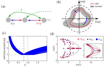
Figure 2: (a) Schematic diagram of the model with next-nearest-neighbor hopping (green lines). (b) The schematic plots of $Re[\beta_{min}]$ versus $Im[\beta_{min}]$ for clean (red solid line) and disordered samples (area in gray). The disorder effect leads to the broadening of $\beta_{min}$ marked by the error-bar. Thus, a unified $|\beta|$ is available as marked in blue solid line. (c) $\ln[\mathcal{F}(E,\beta)]/\min[\ln[\mathcal{F}(E,\beta)]]$ versus $\beta$ for disorder strength $W=7$. The red dashed line presents the overlap of $\beta_{min}$ for different eigenvalues. (d) $Re[E]$ versus $Im[E]$ under PBC (black dots), OBC (blue dots) and GBZ [PBC with $\beta=0.77$ (red dashed line in (c))] (red circles). Inset is the plot for clean samples with $\beta\approx 0.854$, which gives rise to the BBC for $E\approx-0.2\pm 1.6i$. We fix $t=1$, $\gamma=1.4$ and $N=60$.

Nevertheless, after considering disorder effects, the broadening of $\beta_{min}$ will significantly alter the plot of $Re(\beta)$ versus $Im(\beta)$. To identify the unified transformation coefficient, we calculate the $\mathcal{F}(E,\beta)$ versus $\beta$ for each eigenvalue $E$. As shown in Fig.2(c), the interval of $\beta_{min}(E)$ is determined by requiring $\ln\{\mathcal{F}(E,\beta_{min})\}/\min\{\ln[\mathcal{F}(E,\beta_{min})]\}\approx 1$. Remarkably, all the $\beta_{min}(E)$ intersect at a single point, i.e. $\cap_{i\in E}\beta_{min}(i)=0.77$. Since $\beta_{min}(E)$ ensures the BBC for the eigenvalue $E$, the transformed Hamiltonian $\mathcal{H_{GBZ}}$ with $\beta=0.77$ will capture all the eigenvalues under OBC [see Fig. 2(d)]. The interplay between disorder effects and the BBC unveils one of the exotic properties of non-Hermitian systems.

IV application of the modified GBZ theory under magnetic field

In this section, we apply the modified GBZ theory to systems with magnetic field. The Hamiltonian reads:

$$\begin{split}\mathcal{H}=&\sum_{x,y}t^{\pm}c^{\dagger}_{x,y}c_{x\pm\delta_{x},y}+t_{y}e^{\pm i\phi x}c^{\dagger}_{x,y}c_{x,y\pm\delta_{y}}.\end{split}$$ (7)

$\phi$ represents the magnetic flux. Recently, Lu, et. al. and Shao, et. al. both noticed that the strength of NHSE is significantly suppressed Mag1 ; Mag2 by increasing $\phi$. However, the strength of NHSE under the magnetic field cannot be correctly described by the conventional GBZ theory Mag1 . The conventional GBZ theory seems to indicate that the NHSE is irrelevant to the magnetic field. Since such a model is roughly equivalent to a one-dimensional model with the on-site disorder QusiC , we next elucidate that a faithful description of NHSE is still available based on the proposed modified GBZ theory.

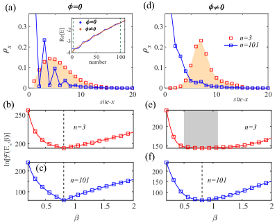
Figure 3: (a) The plot of eigenstates $\rho_{x;n}=\sum_{y}|\psi_{n}(x,y)|^{2}$ versus site $x$ for $n=3$ and $n=101$ with $\phi=0$. Inset plots the real eigenvalues ($Re[E]$) for $\phi=0$ (blue dots) and $\phi=2\pi/(N-1)$ (red dots), which determines the choices of $n$. (b) and (c) $\mathcal{F}(E_{n},\beta)$ versus $\beta$ for $n=3$ and $n=101$, respectively. (d)-(f) are the same with (a)-(c), except $\phi=2\pi/(N-1)$. We set $t^{+}=1.2$, $t^{-}=0.8$, $t_{y}=1$ and $N_{x}=N_{y}=N=20$.

The eigen-equation gives rise to $\mathcal{H}\psi_{n}=E_{n}\psi_{n}(x,y)$. $E_{n}$ stands for the $n_{th}$ eigenvalue shown in the inset of Fig. 3(a). For clarity, we take $n=3$ and $n=101$ as two typical examples. To unveil the universality of the modified GBZ theory under magnetic field, we pay our attention to the evolution of $\mathcal{F}(E_{n},\beta)$ versus $\beta$. When magnetic field is absent, the eigenvectors for $n=3$ and $n=101$ should both show the NHSE’s features, where a single point of $\beta_{min}\sim 0.81$ is obtained based on $\mathcal{F}(E_{n},\beta)$ [see Figs. 3(b)-(c)]. After considering the influence of $\phi$, we notice that $\mathcal{F}(E_{n},\beta)$ gives a plateau for $n=3$ with $\beta_{min}\in[0.5,1.1]$. Based on the modified GBZ theory, the $\beta_{min}=1$ should be adopted to characterize the NHSE, and the NHSE for $n=3$ should be destroyed. On the contrary, a single point with $\beta_{min}\sim 0.81$ is still available for $n=101$. These results are consistent with the plot of eigenvectors in Figs. 3(a) and (d). The NHSE for $n=3$ is destroyed with $n=101$ unaffected by increasing $\phi$, which manifests the magnetic-field-suppressed NHSE.

We close this section by clarifying why the GBZ theory fails to describe the NHSE. The modified GBZ theory considers the influence of $\mathcal{F}_{1}$ on the polynomial $\mathcal{F}(E,\beta)$, which smoothes its sharp dip. Nevertheless, such a process leaves the global minimum of $\mathcal{F}(E,\beta)$ unaffected. The applied GBZ theory in the previous study Mag1 only concentrated on the global minimum, which is almost unaffected by the magnetic field [see Fig. 3(e), the global minimum still gives $\beta\sim 0.8$]. However, the plateau of $\mathcal{F}(E_{n=3},\beta)$ suggests that both $\beta\in[0.5,1.1]$ can capture the minimum of $\mathcal{F}(E_{n=3},\beta)$ and the BBC with high accuracy. In short, a faithful description of NHSE should pay attention to not only the BBC, but also the additional restrictions of the modified GBZ theory.

V summary

In summary, we found the minimum of $\mathcal{F}(E,\beta)$ gives an interval instead of a single point, which eases the realization of BBC. Due to the extended choices of $\beta_{min}$, the unified transformation coefficient $\beta$ for samples with long-range hopping can be obtained. To compare the NHSEs for different cases and eliminate the ambiguous, the strength of NHSEs is unified to the minimum of $|\beta_{min}-1|$. Notably, the modified GBZ theory under strong on-site disorders should concentrate on two key points: (1) the transformation coefficient $\beta=\beta_{min}$ should ensure the correctness of BBC by minimizing $\mathcal{F}(E,\beta)$; (2) $|\beta_{min}-1|$ should also be minimized. Finally, we clarified the paradox of magnetic-irrelevant NHSEs with the help of the modified GBZ theory. Our work deepens the understanding of the characterization of NHSE for samples with on-site disorder and extends the application of the GBZ theory.

VI ACKNOWLEDGEMENT

We are grateful for the valuable discussions with Qiang Wei, Shuguang Cheng and Jing Yu. This work was supported by the National Basic Research Program of China (Grant No. 2019YFA0308403), NSFC under Grant No. 11822407 and No. 12147126, and a Project Funded by the Priority Academic Program Development of Jiangsu Higher Education Institutions.

VII APPENDIX: The Derivation of Eq. (5)

We give the derivation of the analytical formula of $\mathcal{F}_{1}$. For Eq. (4), we mark $t^{+/-}\rightarrow(E-E_{i})\neq 0$ since there is a high probability $t^{+/-}\sim(E-E_{i})$. Here, we suppose $E_{i}$ and $E$ are the eigenvalue of $\mathcal{H}_{\mathcal{OBC};N-2\times N-2}$ and $\mathcal{H}_{\mathcal{OBC};N\times N}$, respectively. One should also notice that the eigenvalue of $\mathcal{H}_{\mathcal{OBC};N\times N}$ is also approximately the eigenvalue of $\mathcal{H}_{\mathcal{OBC};N-2\times N-2}$, and only a slight deviation $\delta=|E_{\mathcal{OBC};N}-E_{\mathcal{OBC};N-2}|\rightarrow 0$ exists. By considering $\delta$, the analytical formula of $\mathcal{F}_{1}$ is obtained

$$\begin{split}&\ln(\mathcal{F}_{1})\approx\sum_{i=1}^{N}\ln(E-E_{i})\\ &=\lim_{\delta\rightarrow 0}\frac{N}{W}[\int_{-\frac{W}{2}}^{E-\delta}\ln(E-x)dx+\int_{E+\delta}^{\frac{W}{2}}\ln(E-x)dx]\\ &=\ln\{[(E-\frac{W}{2})^{(\frac{1}{2}-\frac{E}{W})}(E+\frac{W}{2})^{(\frac{1}{2}+\frac{E}{W})}e^{-1}]^{N}\}.\end{split}$$ (8)

In the above deviation, we require $E_{i}\rightarrow x$ and $|E-E_{i}|>\delta$ for arbitrary $E_{i}\in[-\frac{W}{2},\frac{W}{2}]$.

References

- (1) Y. Ashida, Z. P. Gong, and M. Ueda, Non-hermitian physics, Adv. Phys. 69 249-435 (2020).
- (2) F. K. Kunst and V. Dwivedi, Non-Hermitian systems and topology: A transfer-matrix perspective, Phys. Rev. B 99, 245116 (2019).
- (3) T. Helbig, T. Hofma, S. Imhof, M. Abdelghany, T. Kiessling, L. W. Molenkamp, C. H. Lee, A. Szameit, M. Greiter, and R. Thomale, Generalized bulk-boundary correspondence in non-Hermitian topolectrical circuits, Nat. Phys. 16, 747 (2020).
- (4) R. El-Ganainy, K. G. Makris, M. Khajavikhan, Z. H. Musslimani, S. Rotter, and D. N. Christodoulides, Non-Hermitian physics and PT symmetry, Nat. Phys. 14, 11-19 (2018).
- (5) T. E. Lee, Anomalous edge state in a non-Hermitian lattice, Phys. Rev. Lett. 116, 133903 (2016).
- (6) K. Wang, A. Dutt, C. C. Wojcik, and S. H. Fan, Topological complex-energy braiding of non-Hermitian bands, Nature 598, 59-64 (2021).
- (7) E. Edvardsson, F. K. Kunst, T. Yoshida, and E. J. Bergholtz, Phase transitions and generalized biorthogonal polarization in non-Hermitian systems, Phys. Rev. Research 2, 043046 (2020).
- (8) M. Ezawa, Non-Hermitian higher-order topological states in nonreciprocal and reciprocal systems with their electric-circuit realization, Phys. Rev. B 99, 201411 (2019).
- (9) Z. S. Yang, K. Zhang, C. Fang, and J. P. Hu, Non-hermitian bulk-boundary correspondence and auxiliary generalized brillouin zone theory, Phys. Rev. Lett. 125, 226402 (2020).
- (10) A. Ghatak and T. Das, New topological invariants in non-Hermitian systems, Jour. Phys.: Condens. Matter 31, 263001 (2019).
- (11) V. M. Martinez Alvarez, J. E. Barrios Vargas, M. Berdakin, and L. E. F. Foa Torres, Topological states of non-Hermitian systems, Eur. Phys. J. Special Topics 227, 1295-1308 (2018).
- (12) Z. P. Gong, Y. Ashida, K. Kawabata, K. Takasan, S. Higashikawa, and M. Ueda, Topological phases of non-Hermitian systems, Phys. Rev. X 8, 031079 (2018).
- (13) J. Y. Lee, J. Ahn, H. Zhou, and A. Vishwanath, Topological correspondence between Hermitian and non-Hermitian systems: Anomalous dynamics, Phys. Rev. Lett. 123, 206404 (2019).
- (14) D. Leykam, K. Y. Bliokh, C. Huang, Y. D. Chong, and F. Nori, Edge modes, degeneracies, and topological numbers in non-Hermitian systems, Phys. Rev. Lett. 118, 040401 (2017).
- (15) D. S. Borgnia, A. J. Kruchkov, and R. J. Slager, Non-Hermitian boundary modes and topology, Phys. Rev. Lett. 124, 056802 (2020).
- (16) T. Liu, Y. R. Zhang, Q. Ai, Z. P. Gong, K. Kawabata, M. Ueda, and F. Nori, Second-order topological phases in non-Hermitian systems, Phys. Rev. Lett. 122, 076801 (2019).
- (17) S. Ken and S. Ono, Symmetry indicator in non-Hermitian systems, Phys. Rev. B 104, 035424 (2021).
- (18) C. H. Liu, H. Jiang, and S. Chen, Topological classification of non-Hermitian systems with reflection symmetry, Phys. Rev. B 99, 125103 (2019).
- (19) K. Kawabata, K. Shiozaki, M. Ueda, and M. Sato, Symmetry and topology in non-Hermitian physics, Phys. Rev. X 9, 041015 (2019).
- (20) F. Song, S. Y. Yao, and Z. Wang, Non-Hermitian topological invariants in real space, Phys. Rev. Lett. 123, 246801 (2019).
- (21) S. Y. Yao, F. Song, and Z. Wang, Non-hermitian chern bands, Phys. Rev. Lett. 121, 136802 (2018).
- (22) H. T. Shen, B. Zhen, and L. Fu, Topological band theory for non-Hermitian Hamiltonians, Phys. Rev. Lett. 120, 146402 (2018).
- (23) K. Wang, A. Dutt, K. Y. Yang, C. C. Wojcik, J. Vuckovic, and S. Fan, Generating arbitrary topological windings of a non-Hermitian band, Science, 371, 1240-1245 (2021).
- (24) T. S. Deng and W. Yi, Non-Bloch topological invariants in a non-Hermitian domain wall system, Phys. Rev. B 100, 035102 (2019).
- (25) S. Liu, S. J. Ma, C. Yang, L. Zhang, W. L. Gao, Y. J. Xiang, T. J. Cui, and S. Zhang, Gain-and loss-induced topological insulating phase in a non-Hermitian electrical circuit, Phys. Rev. Applied 13, 014047 (2020).
- (26) Q. B. Zeng and Y. Xu, Winding numbers and generalized mobility edges in non-Hermitian systems, Phys. Rev. Research 2, 033052 (2020).
- (27) J. Claes and T. L. Hughes, Skin effect and winding number in disordered non-Hermitian systems, Phys. Rev. B 103, L140201 (2021).
- (28) X. L. Luo, Z. Y. Xiao, K. Kawabata, T. Ohtsuki, R. Shindou, Unifying the Anderson Transitions in Hermitian and Non-Hermitian Systems, arXiv:2105.02514 (2021).
- (29) D. W. Zhang, L. Z. Tang, L. J. Lang, H. Yan, and S. L. Zhu, Non-hermitian topological anderson insulators, Sci. China-Phys. Mech. Astron. 63, 1-11 (2020).
- (30) X. L. Luo, T. Ohtsuki, and R. Shindou, Universality classes of the Anderson transitions driven by non-Hermitian disorder, Phys. Rev. Lett. 126, 090402 (2021).
- (31) H. F. Liu, Z. X. Su, Z. Q. Zhang, and H. Jiang, Topological Anderson insulator in two-dimensional non-Hermitian systems, Chin. Phys. B 29, 050502 (2020).
- (32) Y. Huang and B. I. Shklovskii, Anderson transition in three-dimensional systems with non-Hermitian disorder, Phys. Rev. B 101, 014204 (2020).
- (33) A. F. Tzortzakakis, K. G. Makris, and E. N. Economou, Non-Hermitian disorder in two-dimensional optical lattices, Phys. Rev. B 101, 014202 (2020).
- (34) L. Z. Tang, L. F. Zhang, G. Q. Zhang, and D. W. Zhang, Topological Anderson insulators in two-dimensional non-Hermitian disordered systems, Phys. Rev. A 101, 063612 (2020).
- (35) H. F. Liu, J. K. Zhou, B. L. Wu, Z. Q. Zhang, and H. Jiang, Real-space topological invariant and higher-order topological Anderson insulator in two-dimensional non-Hermitian systems, Phys. Rev. B 103, 224203 (2021).
- (36) Z. Q. Zhang, H. F. Liu, H. W. Liu, H. Jiang, and X. C. Xie, Bulk-Bulk Correspondence in Disordered Non-Hermitian Systems, arXiv:2201.01577.
- (37) M. Lu, X. X. Zhang, and M. Franz, Magnetic suppression of non-Hermitian skin effects, Phys. Rev. Lett. 127, 256402 (2021).
- (38) K. Shao, H. Geng, W. Chen, and D. Y. Xing, Interplay between non-Hermitian skin effect and magnetic field: skin modes suppression, Onsager quantization and MT phase transition, arXiv:2111.04412.
- (39) Y. Peng, J. Jie, D. Yu, and Y. Wang, Manipulating non-Hermitian skin effect via electric fields, arXiv:2201.10318.
- (40) E. J. Bergholtz, J. C. Budich, and F. K. Kunst, Exceptional topology of non-Hermitian systems, Rev. Mod. Phys. 93, 015005 (2021).
- (41) J. C. Budich, J. Carlstrm, F. K. Kunst, and E. J. Bergholtz, Symmetry-protected nodal phases in non-Hermitian systems, Phys. Rev. B 99, 041406 (2019).
- (42) J. Carlstrm and E. J. Bergholtz, Exceptional links and twisted Fermi ribbons in non-Hermitian systems, Phys. Rev. A 98, 042114 (2018).
- (43) J. Carlstrm, M. Stlhammar, J. C. Budich, and E. J. Bergholtz, Knotted non-Hermitian metals, Phys. Rev. B 99, 161115 (2019).
- (44) R. Okugawa and T. Yokoyama, Topological exceptional surfaces in non-Hermitian systems with parity-time and parity-particle-hole symmetries, Phys. Rev. B 99, 041202 (2019).
- (45) Z. S. Yang, A. P. Schnyder, J. P. Hu, C. K. Chiu, Fermion doubling theorems in two-dimensional non-Hermitian systems for Fermi points and exceptional points, Phys. Rev. Lett. 126, 086401 (2021).
- (46) Z. S. Yang and J. P. Hu, Non-Hermitian Hopf-link exceptional line semimetals, Phys. Rev. B 99, 081102 (2019).
- (47) W. Zhu, X. Fang, D. Li, Y. Sun, Y. Li, Y. Jing, and H. Chen, Simultaneous observation of a topological edge state and exceptional point in an open and non-Hermitian acoustic system, Phys. Rev. Lett. 121, 124501 (2018).
- (48) H. P. Hu and E. H. Zhao, Knots and non-Hermitian Bloch bands, Phys. Rev. Lett. 126, 010401 (2021).
- (49) K. Yokomizo and S. Murakami, Topological semimetal phase with exceptional points in one-dimensional non-Hermitian systems, Phys. Rev. Research 2, 043045 (2020).
- (50) W. Hu, H. Wang, P. P. Shum, and Y. D. Chong, Exceptional points in a non-Hermitian topological pump, Phys. Rev. B 95, 184306 (2017).
- (51) V. M. M. Alvarez, J. E. B. Vargas, and L. E. F. F. Torres, Non-Hermitian robust edge states in one dimension: Anomalous localization and eigenspace condensation at exceptional points, Phys. Rev. B 97, 121401 (2018).
- (52) K. Sone, Y. Ashida, and T. Sagawa, Exceptional non-Hermitian topological edge mode and its application to active matter, Nat. Commun. 11, 1-11 (2020).
- (53) L. H. Li and C. H. Lee, Non-Hermitian Pseudo-Gaps, Science Bulletin (2022).
- (54) N, Matsumoto, K, Kawabata, Y, Ashida, S, Furukawa, and M, Ueda, Continuous phase transition without gap closing in non-Hermitian quantum many-body systems, Phys. Rev. Lett. 125, 260601 (2020).
- (55) F. K. Kunst, E. Edvardsson, J. C. Budich, and E. J. Bergholtz, Biorthogonal bulk-boundary correspondence in non-Hermitian systems, Phys. Rev. Lett. 121, 026808 (2018).
- (56) K. Yokomizo and S. Murakami, Non-bloch band theory of non-hermitian systems, Phys. Rev. Lett. 123, 066404 (2019).
- (57) S. Y. Yao and Z. Wang, Edge states and topological invariants of non-Hermitian systems, Phys. Rev. Lett. 121 086803 (2018).
- (58) F. Song, S. Y. Yao, and Z, Wang, Non-Hermitian skin effect and chiral damping in open quantum systems, Phys. Rev. Lett. 123, 170401 (2019).
- (59) X. Ye, Why does bulk boundary correspondence fail in some non-hermitian topological models, J. Phys. Commun. 2, 035043 (2018).
- (60) C. H. Lee and R. Thomale, Anatomy of skin modes and topology in non-Hermitian systems, Phys. Rev. B 99, 201103 (2019).
- (61) Z. Kai, Z. S. Yang, and C. Fang, Correspondence between winding numbers and skin modes in non-Hermitian systems, Phys. Rev. Lett. 125, 126402 (2020).
- (62) L. H. Li, C. H. Lee, S. Mu, and J. B. Gong, Critical non-Hermitian skin effect, Nat. Commun. 11, 1-8 (2020).
- (63) N. Okuma, K. Kawabata, K. Shiozaki, and M. Sato, Topological origin of non-Hermitian skin effects, Phys. Rev. Lett. 124, 086801 (2020).
- (64) X. Q. Sun, P. H. Zhu, and T. L. Hughes, Geometric response and disclination-induced skin effects in non-Hermitian systems, Phys. Rev. Lett. 127, 066401 (2021).
- (65) S. Liu , R. W. Shao, S. J. Ma, L. Zhang, O. B. You, H. T. Wu, Y. J. Xiang, T. J. Cui, and S, Zhang, Non-Hermitian skin effect in a non-Hermitian electrical circuit, Research 2021, (2021).
- (66) K. Kawabata, M. Sato, and K. Shiozaki, Higher-order non-Hermitian skin effect, Phys. Rev. B 102, 205118 (2020).
- (67) Y. F. Yi and Z. S. Yang, Non-Hermitian skin modes induced by on-site dissipations and chiral tunneling effect, Phys. Rev. Lett. 125, 186802 (2020).
- (68) C. X. Guo, C. H. Liu, X. M. Zhao, Y. Liu, and S. Chen , Exact solution of non-hermitian systems with generalized boundary conditions: Size-dependent boundary effect and fragility of the skin effect, Phys. Rev. Lett. 127, 116801 (2021).
- (69) C. Yuce, Non-Hermitian anomalous skin effect, Phys. Lett. A 384, 126094 (2020).
- (70) Y. X. Fu, J. H. Hu, and S. L. Wan, Non-Hermitian second-order skin and topological modes, Phys. Rev. B 103, 045420 (2021).
- (71) K. Yokomizo and S. Murakami, Scaling rule for the critical non-Hermitian skin effect, Phys. Rev. B 104, 165117 (2021).
- (72) R. Okugawa, R. Takahashi, and K. Yokomizo, Second-order topological non-Hermitian skin effects, Phys. Rev. B 102, 241202 (2020).
- (73) X. Y. Zhu, H. Q. Wang, S. K. Gupta, H. J. Zhang, B. Xie, M. H. Lu, and Y. F. Chen, Photonic non-Hermitian skin effect and non-Bloch bulk-boundary correspondence, Phys. Rev. Research 2, 013280 (2020).
- (74) X. Zhang, Y. Tian, J. H. Jiang, M. H. Lu, and Y. F. Chen, Observation of higher-order non-Hermitian skin effect, Nat. Commun. 12, 1-8 (2021).
- (75) K. Zhang, Z. S. Yang, and C. Fang, Universal non-Hermitian skin effect in two and higher dimensions, arXiv:2102.05059.
- (76) N. Okuma and M. Sato, Non-hermitian skin effects in hermitian correlated or disordered systems: Quantities sensitive or insensitive to boundary effects and pseudo-quantum-number, Phys. Rev. Lett. 126, 176601 (2021).
- (77) Y. Song, W. Liu, L. Zheng, Y. Zhang, B. Wang, and P, Lu, Two-dimensional non-Hermitian skin effect in a synthetic photonic lattice, Phys. Rev. Applied 14, 064076 (2020).
- (78) S. Longhi, Non-Hermitian skin effect beyond the tight-binding models, Phys. Rev. B 104, 125109 (2021).
- (79) H. W. Li, X. L. Cui, and W. Yi, Non-Hermitian skin effect in a spin-orbit-coupled Bose-Einstein condensate, arXiv:2201.01580.
- (80) C. H. Lee, L. Li, and J. B. Gong, Hybrid Higher-Order Skin-Topological Modes in Nonreciprocal Systems, Phys. Rev. Lett. 123, 016805 (2019).
- (81) R. Sarkar, S. S. Hegde, and A. Narayan, Interplay of disorder and point-gap topology: Chiral modes, localization, and non-Hermitian Anderson skin effect in one dimension, Phys. Rev. B 106, 014207 (2022).
- (82) Yaacov E. Kraus, Yoav Lahini, Zohar Ringel, Mor Verbin, and Oded Zilberberg, Topological States and Adiabatic Pumping in Quasicrystals, Phys. Rev. Lett. 109, 106402 (2012).
- (83) N. Hatano and D. R. Nelson, Localization transitions in non-Hermitian quantum mechanics, Phys. Rev. Lett. 77, 570 (1996).
- (84) P. W. Anderson, Absence of diffusion in certain random lattices, Phys. Rev. 109, 1492 (1958).