Multipole moments on the common horizon in a binary-black-hole simulation

Abstract

We construct the covariantly defined multipole moments on the common horizon of an equal-mass, non-spinning, quasicircular binary-black-hole system. We see a strong correlation between these multipole moments and the gravitational waveform. We find that the multipole moments are well described by the fundamental quasinormal modes at sufficiently late times. For each multipole moment, at least two fundamental modes of different $\ell$ are detectable in the best model. These models provide faithful estimates of the true mass and spin of the remnant black hole. We also show that by including overtones, the $\ell=m=2$ mass multipole moment admits an excellent quasinormal-mode description at all times after the merger. This demonstrates the perhaps surprising power of perturbation theory near the merger.

I Introduction

The black hole (BH) no-hair theorem [1, 2] suggests that the final state of a charge-neutral BH merger satisfies the Kerr solution, which is characterized by only two parameters: mass and angular momentum (or equivalently, spin). Numerical simulations of binary-black-hole (BBH) systems have directly confirmed this theorem by comparing the quantities in the final stage with the corresponding Kerr values [3, 4, 5, 6]. The Kerr spacetime is axisymmetric and has a simple geometry. In stark contrast, as brought out by numerical simulations, the horizon of a merged BH is highly distorted at its formation, and undergoes large dynamical changes as it approaches equilibrium. For a BH merger to lose its hair and settle down to the final Kerr state, the horizon distortion must be washed away by general relativity in the ringdown phase.

In numerical relativity, an event horizon is not a convenient notion of horizon, as it cannot be determined during the evolution of the spacetime. It is typically found in post-processing, once the complete spacetime is known. Quasilocal objects like apparent horizons are more favored, because they can be computed on each time slice without the knowledge of the complete spacetime. A recent topic in the study of quasilocal objects is seeking a quantitative description of the horizon behavior of a BBH merger. One of the physical quantities used for such an investigation is the gravitational flux falling into a horizon. It turns out that the infalling energy flux is correlated with the outgoing flux of gravitational waves [7, 8]. This might seem slightly surprising at first glance but is indeed reasonable, because both the ingoing and outgoing flux are generated from the same gravitational source. Besides the flux, another quantity that can be used in the analysis of BH horizons is the set of horizon multipole moments. In the following discussion, we will discuss the multipole moments only in the ringdown phase, though this concept is also applicable in the inspiral phase (see, e.g., Ref. [9]).

Horizon multipole moments generalize the mass and spin of a BH. It is fairly straightforward to define multipole moments on the isolated horizon of a Kerr BH [10], or on a dynamical horizon that is axisymmetric throughout the whole ringdown phase [11]. This is because in both situations, the horizon possesses a rotational Killing vector, which is associated with a natural choice of angular coordinates. In a more general BBH configuration, however, choosing an appropriate definition of multipole moments is a nontrivial task. One difficulty comes from the nonaxisymmetry of the dynamical horizon. Moreover, the coordinate system used to express the components of spacetime quantities varies from simulations to simulations, which calls for an invariant notion of multipole moments. Ashtekar et al. [12] provide a definition of horizon multipole moments that is appropriate for this task. They start with the axisymmetry of the final BH, construct weighting fields subject to this axisymmetry, and transport these weighting fields backward along the dynamical horizon. The resulting multipole moments are then spatially gauge independent on a given dynamical horizon. This set of multipole moments will be the subject of this paper, and we will explain the construction process in greater detail in later sections.

Regardless of different notions of multipole moments, an important goal in studying them is to discover any universality in the horizon behavior of a remnant BH. A natural avenue is to find inspiration from multipole moments of the gravitational waveform in the ringdown phase. BH perturbation theory shows that the gravitational waves radiated by a perturbed BH at late times can be characterized by a superposition of exponentially damped oscillations, called the quasinormal modes (QNMs) [13, 14, 15, 16]. The frequency and the decay constant of each mode are completely determined by the final mass and spin, consistent with the no-hair theorem. The presence of quasinormal modes in the late-time behavior of post-merger waveforms has already been confirmed in numerical simulations (e.g., [17, 18]). Recently, Giesler et al. [19] discovered that including overtones even allows a QNM model to describe the waveform immediately after merger.

Although the waveform multipole moments are a superposition of QNMs in the ringdown phase, we might not expect this behavior in multipole moments of the dynamical horizon soon after the common horizon forms. After all, this horizon is initially highly distorted compared to a Kerr horizon, so we have no reason to expect perturbation theory to be valid. Moreover, the time coordinate of the simulation is quite arbitrary compared to the time coordinate of an observer at infinity, which is used to define the frequency of QNMs. Nevertheless, there is strong evidence supporting the idea that horizon multipole moments exhibit QNM behavior [20, 8, 21, 22]. However, such evidence is based on either the special case of a head-on collision of two BHs, or a definition of multipole moments that does not refer to the connection among quasilocal horizons on different time slices. A definition ignoring the diffeomorphism content of a dynamical horizon is subject to the arbitrariness of spatial coordinates.

In this paper, we calculate the horizon multipole moments that are spatially gauge invariant on the common horizon of an equal-mass BBH system, following the definition in Ref. [12]. To investigate the dynamics of these multipole moments, we test their balance laws, compare them with waveform multipole moments, and model them as linear combinations of QNMs. Regarding the QNM models, we use fundamental tones to analyze the late-time behavior of multipole moments, and then include overtones in the survey of their early-time patterns. We will also consider the effect of mode mixing, which turns out to be significant in most of the multipole moments.

The rest of this paper is structured as follows. In Sec. II, we introduce the notions of horizons and quasinormal modes. We also describe the construction process of the horizon multipole moments proposed by Ashtekar et al. [12]. In Sec. III, we describe the configuration of our BBH simulation and implement the procedure to extract multipole moments on the common horizon. In Sec. IV, we first look for potential correlations between horizon and waveform behavior in the context of their respective multipole moments. Then, we investigate the damped sinusoidal patterns of multipole moments using QNM models, with or without the inclusion of overtones. We finally summarize the results and give remarks on possible future work in Sec. V.

II Preliminaries

II.1 Dynamical horizons

A spacetime is a 4-dimensional Lorentzian manifold $\mathscr{M}$ equipped with a metric $g_{ab}$ of signature $(-,+,+,+)$. Here, we only consider a vacuum spacetime that is asymptotically flat. Let $\nabla_{a}$ be the covariant derivative compatible with $g_{ab}$. Let $\mathcal{S}\subset\mathscr{M}$ be a smooth, orientable, spacelike 2-manifold with spherical topology $S^{2}$. Let $\tilde{q}_{ab}$ be the induced metric on $\mathcal{S}$. (All symbols with tilde in this paper represent quantities on or associated with $\mathcal{S}$.) The outgoing and ingoing future-directed null normals to $\mathcal{S}$, denoted as $l^{a}$ and $n^{a}$, are normalized subject to $l\cdot n=l^{a}n_{a}=-1$. The expansions of $l^{a}$ and $n^{a}$ are

$$\Theta_{(l)} =\tilde{q}^{ab}\nabla_{a}l_{b},$$ (1)

$$\Theta_{(n)} =\tilde{q}^{ab}\nabla_{a}n_{b}.$$ (2)

The shear of $l^{a}$ is

$$\sigma_{ab} =\tilde{q}_{a}^{\ c}\tilde{q}_{b}^{\ d}\nabla_{c}l_{d}-\frac{1}{2}\Theta_{(l)}\tilde{q}_{ab},$$ (3)

while the shear of $n^{a}$ is not used in this paper. Note that $\sigma_{ab}$ is related to but different from the shear spin coefficient $\sigma$, which is usually defined using a complex null tetrad.

A marginally outer trapped surface (MOTS) is a surface $\mathcal{S}$ satisfying $\Theta_{(l)}=0$ (following the convention in Ref. [23]). A MOTS is called a future MOTS if $\Theta_{(n)}<0$, or a past MOTS if $\Theta_{(n)}>0$. The notion of a MOTS is quasilocal, which makes it very convenient because the calculation does not require the knowledge of a full spacetime. In numerical simulations of BHs, there are efficient algorithms [24, 25, 26, 27, 28] that compute MOTSs to locate BHs on every Cauchy surface $\Sigma$.

A marginally trapped tube is a smooth 3-manifold $\mathcal{H}$ foliated by future MOTSs [23]. The 3-manifold $\mathcal{H}$ is said to be a dynamical horizon [31, 30, 32, 23] if it is spacelike, or a timelike membrane if it is timelike. We call $\mathcal{H}$ a non-expanding horizon if it is null [33, 34, 35]. A non-expanding horizon is called an isolated horizon [33, 34, 35] if there is a specific null normal $\mathring{l}^{a}$ to $\mathcal{H}$ such that

$$(\mathcal{L}_{\mathring{l}}D_{a}-D_{a}\mathcal{L}_{\mathring{l}})W^{a}=0,$$ (4)

for any tangent vector $W^{a}$ on $\mathcal{H}$. Here $D_{a}$ is the covariant derivative compatible with the (degenerate) metric $q_{ab}$ induced on $\mathcal{H}$ We are not interested in the specific form of $\mathring{l}^{a}$ on an isolated horizon, though it can be constructed from any null normal (see Sec. IV B in [35]).

After the merger of a BBH, the outermost MOTSs (called the common horizons) on Cauchy surfaces trace out a dynamical horizon. As we expect the remnant BH to be Kerr, this dynamical horizon should asymptote to an axisymmetric isolated horizon [33] as the BH settles down. We are only interested in this dynamical horizon (which is, the stack of common horizons) in the rest of this paper, so we reserve the symbol $\mathcal{H}$ to represent this dynamical horizon henceforth.

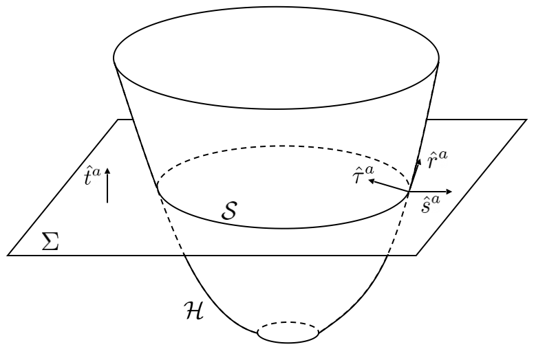
Figure 1: Dynamical horizon in a numerical simulation. The common horizon $\mathcal{S}$ is computed on the Cauchy surface $\Sigma$ (the horizontal plane). The dynamical horizon $\mathcal{H}$ (the paraboloid) consists of a stack of $\mathcal{S}$. Note that these shapes do not reflect the actual appearance of these quantities. See Sec. II.1 for the definitions of the vectors. This figure is a modification of Fig. 1 of Ref. [12].

We visualize the relation among $\mathcal{S}$, $\mathcal{H}$, and $\Sigma$ in Fig. 1. The figure is based on Fig. 1 of Ref. [12], with slightly different use of symbols. This figure is merely illustrative: the shapes of the objects in this figure do not reflect their actual appearance in a numerical simulation. The horizontal plane represents a Cauchy surface $\Sigma$, and the circle on this plane represents the common horizon $\mathcal{S}$. The common horizons on all Cauchy surfaces constitute a dynamical horizon $\mathcal{H}$, shown as the paraboloid. There are four vectors in this figure: $\hat{t}^{a}$ is the unit timelike normal to $\Sigma$, $\hat{\tau}^{a}$ the unit timelike normal to $\mathcal{H}$ within the spacetime, $\hat{r}^{a}$ the unit spacelike normal to $\mathcal{S}$ within $\mathcal{H}$, and $\hat{s}^{a}$ the unit spacelike normal to $\mathcal{S}$ within $\Sigma$. Based on these unit vectors, we fix the scaling freedom in $l\cdot n=-1$ by choosing

$$l^{a}=\hat{\tau}^{a}+\hat{r}^{a},\qquad n^{a}=\frac{1}{2}(\hat{\tau}^{a}-\hat{r}^{a}).$$ (5)

We also define another set of null normals that satisfy the same normalization, {$l^{\prime},n^{\prime}$}, such that

$$l^{\prime a}=\hat{t}^{a}+\hat{s}^{a},\qquad n^{\prime a}=\frac{1}{2}(\hat{t}^{a}-\hat{s}^{a}).$$ (6)

II.2 Multipole moments

The notion of multipole moments on horizons was first introduced for an isolated horizon [10]. If an isolated horizon is axisymmetric, multipole moments are defined as the multipolar expansion of the Weyl scalar $\Psi_{2}$. Multipole moments were later generalized to a dynamical horizon in Refs. [11, 20, 12]. As mentioned in the previous section, we only consider a dynamical horizon $\mathcal{H}$ that asymptotes to an axisymmetric isolated horizon. In simulations, the late portion of $\mathcal{H}$ can be treated as an axisymmetric isolated horizon to within numerical accuracy. We construct multipole moments on such a dynamical horizon by following Ref. [12].

II.2.1 Multipole moments on an axisymmetric $\mathcal{S}$

We start by choosing a pair of angular coordinates $(\theta,\phi)$ on $\mathcal{S}$. If $\mathcal{S}$ is axisymmetric (as in the late portion of $\mathcal{H}$), there is a natural choice of $(\theta,\phi)$ [10]. Let $\varphi^{a}$ on $\mathcal{S}$ be the rotational Killing vector field, which generates closed integral curves and vanishes at exactly two points (the poles). Let $\phi$ be the affine parameter of each closed integral curve with range $[0,2\pi)$. We then pick a new curve that connects the two poles and is orthogonal to $\varphi^{a}$ everywhere, and we set it to be the prime meridian $\phi=0$. We define a variable $\zeta$ that satisfies

$$\tilde{D}_{a}\zeta=\frac{1}{R^{2}}\tilde{\epsilon}_{ba}\varphi^{b},$$ (7)

$$\oint_{\mathcal{S}}\zeta d^{2}V=0,$$ (8)

where $\tilde{D}_{a}$ is the covariant derivative compatible with $\tilde{q}_{ab}$, $\tilde{\epsilon}_{ab}$ the area 2-form, $d^{2}V$ the corresponding area element, $R=\sqrt{A/4\pi}$ the areal radius, and $A$ the area. It is necessary that $\zeta$ has range $[-1,1]$. We obtain the angle $\theta$ via $\zeta=\cos\theta$. Note that there is a rotational degree of freedom in choosing the prime meridian, and we will fix this freedom in Sec. III.1.

In the $(\theta,\phi)$ coordinates, the induced metric on $\mathcal{S}$ can be written as [10]

$$\tilde{q}_{ab} =\frac{R^{4}\sin^{2}\theta}{|\vec{\varphi}|^{2}}(d\theta)_{a}(d\theta)_{b}+|\vec{\varphi}|^{2}(d\phi)_{a}(d\phi)_{b},$$ (9)

where $|\vec{\varphi}|^{2}=\varphi^{a}\varphi_{a}$. The compatible area element, $d^{2}V=R^{2}\sin\theta d\theta d\phi$, is the same as the area element of a fictitious round 2-sphere metric,

$$\mathring{q}_{ab} =R^{2}[(d\theta)_{a}(d\theta)_{b}+\sin^{2}\theta(d\phi)_{a}(d\phi)_{b}].$$ (10)

Spherical harmonics are then defined as usual,

$$Y_{\ell m}(\theta,\phi)=\sqrt{\frac{2\ell+1}{4\pi}\frac{(\ell-m)!}{(\ell+m)!}}P_{\ell}^{m}(\cos\theta)e^{im\phi},$$ (11)

where $P_{\ell}^{m}(x)$ are the associated Legendre polynomials (with the Condon–Shortley phase convention) [36]. These $Y_{\ell m}$ are orthogonal on $\mathcal{S}$:

$$\oint_{\mathcal{S}}Y^{*}_{\ell m}Y_{\ell^{\prime}m^{\prime}}d^{2}V=R^{2}\delta_{\ell\ell^{\prime}}\delta_{mm^{\prime}},$$ (12)

where * denotes complex conjugation, and the integration is with respect to the area 2-form of $\tilde{q}_{ab}$.

On an axisymmetric $\mathcal{S}$, we define mass multipole moments (or simply mass moments) $I_{\ell m}$ and spin multipole moments (spin moments) $L_{\ell m}$ as

$$I_{\ell m} =\frac{1}{4}\oint_{\mathcal{S}}\tilde{\mathcal{R}}Y^{*}_{\ell m}d^{2}V,$$ (13)

$$L_{\ell m} =\frac{1}{2}\oint_{\mathcal{S}}\tilde{\epsilon}^{ab}\tilde{\omega}_{b}\tilde{D}_{a}Y^{*}_{\ell m}d^{2}V.$$ (14)

Here, $\tilde{\mathcal{R}}$ is the $\tilde{q}_{ab}$-compatible Ricci scalar on $\mathcal{S}$, and $\tilde{\omega}_{a}$ is the rotational 1-form,

$$\tilde{\omega}_{a}=-\tilde{q}^{\ b}_{a}n^{c}\nabla_{b}l_{c}.$$ (15)

These multipole moments are related to the Weyl scalar $\Psi_{2}$ by

$$I_{\ell m}+iL_{\ell m} =-\oint_{\mathcal{S}}\Psi_{2}Y^{*}_{\ell m}d^{2}V,$$ (16)

because $\Psi_{2}$ on an isolated horizon satisfies [10]

$$\Psi_{2}=-\frac{1}{4}\tilde{\mathcal{R}}+\frac{i}{2}\tilde{\epsilon}^{ab}\tilde{D}_{a}\tilde{\omega}_{b}.$$ (17)

Although the $m=0$ modes ($I_{\ell,0}$ and $L_{\ell,0}$) are the only nonvanishing modes because of the axisymmetry of $\mathcal{S}$, we keep $m$ arbitrary so that we can easily generalize multipole moments on any MOTS of $\mathcal{H}$ in the coming sections.

At the end of Sec. II.1, we fixed the scaling freedom in {$l,n$}, so there is no ambiguity in the definition of $\tilde{\omega}_{a}$. As the scaling freedom does not affect $\Psi_{2}$ and $L_{\ell m}$, we can replace the current pair {$l,n$} in Eq. (15) by any other null {$l,n$} subject to $l\cdot n=-1$. For the purpose of this paper, it is more convenient and stable to use the pair {$l^{\prime},n^{\prime}$} in the definition of a rotational 1-form. We define

$$\omega_{a}=-\gamma^{\ b}_{a}n^{\prime c}\nabla_{b}l^{\prime}_{c}=\gamma^{\ b}_{a}\hat{s}^{c}\nabla_{b}\hat{t}_{c}=\left(K^{\Sigma}\right)_{ab}\hat{s}^{b},$$ (18)

where $\gamma_{ab}$ is the spatial metric induced on $\Sigma$, and $\left(K^{\Sigma}\right)_{ab}=\gamma_{a}^{\ c}\nabla_{c}\hat{t}_{b}$ is the extrinsic curvature of $\Sigma$ within the spacetime. Replacing $\tilde{\omega}_{a}$ by $\omega_{a}$, we have an equivalent definition of spin moments,

$$L_{\ell m} =\frac{1}{2}\oint_{\mathcal{S}}\tilde{\epsilon}^{ab}\omega_{b}\tilde{D}_{a}Y^{*}_{\ell m}d^{2}V.$$ (19)

It is also useful to rewrite Eq. (19) as

$$L_{\ell m} =-\frac{1}{2}\oint_{\mathcal{S}}\omega_{a}\varphi^{a}_{\ell m}d^{2}V,$$ (20)

$$\varphi^{a}_{\ell m} =\tilde{\epsilon}^{ab}\tilde{D}_{b}Y^{*}_{\ell m}.$$ (21)

The vectors $\varphi^{a}_{\ell m}$ provide a complete basis for divergence-free vectors on $\mathcal{S}$ [12], and the vector $\varphi^{a}_{1,0}$ is parallel to the rotational Killing vector field $\varphi^{a}$ [see Eq. (7)].

II.2.2 2+1 decomposition of $\mathcal{H}$

Except in special situations (e.g., head-on collisions of two BHs), an arbitrary MOTS $\mathcal{S}$ in $\mathcal{H}$ is not axisymmetric. It then becomes tricky to choose a suitable pair of angular coordinates $(\theta,\phi)$. We cannot simply apply the construction process in the previous section, since there is no longer a rotational Killing vector field on an arbitrary $\mathcal{S}$. However, we can still take advantage of the axisymmetry of those $\mathcal{S}$ in the late portion of $\mathcal{H}$. In particular, instead of defining $(\theta,\phi)$ separately and locally on every $\mathcal{S}$, we adopt the idea in Ref. [12] and build a vector $X^{a}$ on $\mathcal{H}$ that connects $(\theta,\phi)$ on all $\mathcal{S}$ in a canonical way. We call $X^{a}$ the stitching vector and regard the coordinates $(\theta,\phi)$ as “evolving” along $X^{a}$ on $\mathcal{H}$.

A dynamical horizon is essentially a stack of MOTSs, so it naturally admits a 2+1 decomposition, similar to a 3+1 decomposition of spacetime (cf. [37] for an introduction of a 3+1 decomposition). Additionally, the foliation by MOTSs is unique for a dynamical horizon, in contrast to a non-expanding horizon [23]. We treat $X^{a}$ as the time vector of the 2+1 decomposition, which has the form,

$$X^{a}=\tilde{\alpha}\hat{r}^{a}+\tilde{\beta}^{a},$$ (22)

where $\tilde{\beta}^{a}$ is a tangent vector to be specified on $\mathcal{S}$. The scalar $\tilde{\alpha}$ and the vector $\tilde{\beta}^{a}$ are the lapse and the shift in this 2+1 decomposition. We call $\tilde{\alpha}$ the 2-lapse and $\tilde{\beta}^{a}$ the 2-shift, to distinguish them from the usual lapse $\alpha$ and shift $\beta^{a}$ used in a 3+1 decomposition.

The 2-lapse is required to preserve the foliation of MOTSs. Let the MOTSs be labeled by a parameter ${v}$ that is smooth on $\mathcal{H}$. In other words, each MOTS corresponds to a ${v}=\mathrm{constant}$ surface. (We will identify ${v}$ with simulation time $t$ in a numerical simulation, but we continue using ${v}$ here to keep the discussion general.) For $X^{a}$ being the time vector, we require ${v}$ to be the parameter of the integral curve generated by $X^{a}$, i.e., $X^{a}=(\partial_{v})^{a}$. This implies

$$\tilde{\alpha}=(q^{ab}D_{a}{v}D_{b}{v})^{-1/2},$$ (23)

where $q_{ab}$ is the induced metric on $\mathcal{H}$, and $D_{a}$ is the covariant derivative compatible with $q_{ab}$. Note that $\tilde{\alpha}$ tends to 0 when $q_{ab}$ approaches a degenerate metric, as in the case when a merged BH approaches equilibrium. However, $X^{a}$ does not tend to 0, because the limiting behavior of $\hat{r}^{a}$ is nontrivial. This brings difficulties in the numerical calculation of $X^{a}$, and we will handle them in the next section.

Spin moments on an isolated horizon (or the late portion of $\mathcal{H}$) can be defined using a set of divergence-free vector fields [Eq. (20)]. This inspires us to define spin moments on a general $\mathcal{S}$ that also uses divergence-free vector fields. We can obtain a canonical set of divergence-free vector fields on all $\mathcal{S}$ by imposing a mapping condition on $X^{a}$: $X^{a}$ maps divergence-free vector fields among different $\mathcal{S}$ isomorphically. Specifically, once $\varphi^{a}_{\ell m}$ (the divergence-free vectors on an axisymmetric $\mathcal{S}$) are known, we can Lie drag them along $X^{a}$ to all other MOTSs. In the mathematical language, we are looking for a vector $X^{a}$ on $\mathcal{H}$, that satisfies the following statement. Given a vector field $\xi^{a}$ that is divergence free on a particular MOTS $\mathcal{S}$, i.e.,

$$\mathcal{L}_{\xi}\tilde{\epsilon}_{ab}\stackrel{{\scriptstyle\mathcal{S}}}{{=}}0,$$ (24)

we can define $\xi^{a}$ on other MOTSs via $\mathcal{L}_{X}\xi^{a}=0$, and the resultant vector field stays divergence free on all MOTSs, i.e.,

$$\mathcal{L}_{\xi}\tilde{\epsilon}_{ab}\stackrel{{\scriptstyle\mathcal{H}}}{{=}}0.$$ (25)

The trivial choice $\tilde{\beta}^{a}=0$ does not satisfy this mapping condition. To see this, we first note that Eq. (25) implies $\mathcal{L}_{X}\mathcal{L}_{\xi}\tilde{\epsilon}_{ab}=0$. Meanwhile, we know $\mathcal{L}_{X}\mathcal{L}_{\xi}\tilde{\epsilon}_{ab}=\mathcal{L}_{\xi}\mathcal{L}_{X}\tilde{\epsilon}_{ab}=\mathcal{L}_{\xi}(\tilde{\alpha}\tilde{K})$ because $\mathcal{L}_{X}\xi^{a}=0$ and $\mathcal{L}_{\tilde{\alpha}\hat{r}}\tilde{\epsilon}_{ab}=\tilde{\alpha}\tilde{K}\tilde{\epsilon}_{ab}$. Here, $\tilde{K}_{ab}=\tilde{q}_{a}^{\ c}\tilde{q}_{b}^{\ d}\nabla_{c}\hat{r}_{d}$ is the extrinsic curvature of $\mathcal{S}$ within $\mathcal{H}$, and $\tilde{K}=\tilde{K}^{a}_{\ a}$ is its trace. The expression $\mathcal{L}_{\xi}(\tilde{\alpha}\tilde{K})$ is generally nonzero, which contradicts $\mathcal{L}_{X}\mathcal{L}_{\xi}\tilde{\epsilon}_{ab}=0$.

We can find a viable choice of $\tilde{\beta}^{a}$ by eliminating the inhomogeneity in $\tilde{\alpha}\tilde{K}$ from $\mathcal{L}_{X}\tilde{\epsilon}_{ab}$. In detail, the inhomogeneity is

$$\tilde{\alpha}\tilde{K}-\frac{1}{4\pi R^{2}}\oint_{\mathcal{S}}\tilde{\alpha}\tilde{K}d^{2}V=\tilde{\alpha}\tilde{K}-\frac{2\dot{R}}{R},$$ (26)

where $\dot{R}=dR/d{v}$. We choose $\tilde{\beta}^{a}$ such that

$$\tilde{D}_{a}\tilde{\beta}^{a}=-(\tilde{\alpha}\tilde{K}-2\dot{R}/R),$$ (27)

which implies $\mathcal{L}_{X}\tilde{\epsilon}_{ab}=(2\dot{R}/R)\tilde{\epsilon}_{ab}$. Note that $2\dot{R}/R$ is only a function of ${v}$. The differential equation $\mathcal{L}_{X}\mathcal{L}_{\xi}\tilde{\epsilon}_{ab}=\mathcal{L}_{\xi}\mathcal{L}_{X}\tilde{\epsilon}_{ab}=(2\dot{R}/R)\mathcal{L}_{\xi}\tilde{\epsilon}_{ab}$, together with the initial condition Eq. (24), admits the unique solution Eq. (25). In other words, this choice of $\tilde{\beta}^{a}$ [Eq. (27)] satisfies the mapping condition of $X^{a}$. In the numerical implementation of Eq. (27), it is more convenient to define

$$\tilde{\beta}^{a}=\tilde{q}^{ab}\tilde{D}_{b}g$$ (28)

and solve

$$\tilde{q}^{ab}\tilde{D}_{a}\tilde{D}_{b}g=-(\tilde{\alpha}\tilde{K}-2\dot{R}/R)$$ (29)

for $g$ on every $\mathcal{S}$. The integration constant in the solution of $g$ does not affect $\tilde{\beta}^{a}$ and can be selected arbitrarily.

We have thus constructed the time vector $X^{a}$ that satisfies the following four properties:

1. $X^{a}$ is constructed covariantly.

2. $X^{a}$ preserves the foliation of $\mathcal{H}$.

3. $X^{a}$ maps divergence-free vectors isomorphically among different $\mathcal{S}$.

4. If $\mathcal{H}$ is axisymmetric, $X^{a}$ preserves the rotational Killing vector.

Now, we are ready to define multipole moments on a general dynamical horizon $\mathcal{H}$ whose late portion is axisymmetric. We first construct $Y_{\ell m}(\theta,\phi)$ on an axisymmetric but otherwise arbitrary $\mathcal{S}$ as described in Sec. II.2.1. We then extend $Y_{\ell m}(\theta,\phi)$ to the whole $\mathcal{H}$ by

$$\mathcal{L}_{X}Y_{\ell m}=0.$$ (30)

We define mass (multipole) moments $I_{\ell m}$ and spin (multipole) moments $L_{\ell m}$ as functions of ${v}$ (or time $t$ in numerical simulations),

$$I_{\ell m} =\frac{1}{4}\oint_{\mathcal{S}}\tilde{\mathcal{R}}Y^{*}_{\ell m}d^{2}V,$$ (31)

$$L_{\ell m} =\frac{1}{2}\oint_{\mathcal{S}}\tilde{\epsilon}^{ab}\omega_{b}\tilde{D}_{a}Y^{*}_{\ell m}d^{2}V,$$ (32)

where $\tilde{\mathcal{R}}$ still represents the $\tilde{q}_{ab}$-compatible Ricci scalar and $\omega_{a}$ is still defined by Eq. (18). These multipole moments are dimensionless, so they are sometimes referred to as geometric multipole moments. They extend Eqs. (13) and (19), but the relation among $\Psi_{2}$, $\tilde{\mathcal{R}}$, and $\tilde{\epsilon}^{ab}\tilde{D}_{a}\tilde{\omega}_{b}$ is not as simple as Eq. (17), so Eq. (16) no longer holds on a general MOTS. Also, see Refs. [20, 12] for other definitions of multipole moments on a dynamical horizon.

II.2.3 Alternative calculation of $X^{a}$

The 2+1 decomposition, Eq. (22), nicely resembles the 3+1 decomposition of a spacetime, but there exist numerical difficulties in the implementation. For example, as $\mathcal{H}$ becomes null and $q_{ab}$ becomes degenerate, $\tilde{\alpha}$ tends to zero and the components of $\hat{r}^{a}$ diverge. References [30, 12] discuss these ill behaviors and provide an alternative solution to handle them. Using this alternative solution, we can compute $X^{a}$ stably on both dynamical and isolated horizons, as described below.

Let $V^{a}$ be a normal to $\mathcal{S}$ within $\mathcal{H}$ such that

$$V^{a}D_{a}{v}=1.$$ (34)

The vector $V^{a}$ is unique and well defined on both dynamical and isolated horizons. It is null on an isolated horizon and reduces to the spacelike vector $\tilde{\alpha}\hat{r}^{a}$ on a dynamical horizon. Thus, it is more promising to use

$$X^{a}=V^{a}+\tilde{\beta}^{a}$$ (35)

in numerical simulations. The 2-shift $\tilde{\beta}^{a}$ may also be problematic because of its dependence on $\tilde{\alpha}$ and $\tilde{K}$ [Eq. (29)]. As $\mathcal{H}$ becomes null, evaluating $\tilde{\alpha}$ and $\tilde{K}$ may become unstable. A better way to obtain $\tilde{\beta}^{a}$ is to use the following differential equation for $g$,

$$\tilde{q}^{ab}\tilde{D}_{a}\tilde{D}_{b}g=-(\frac{1}{2}\tilde{q}^{ab}\mathcal{L}_{V}\tilde{q}_{ab}-\frac{2\dot{R}}{R}).$$ (36)

This generalizes Eq. (29), because $\tilde{q}^{ab}\mathcal{L}_{V}\tilde{q}_{ab}$ reduces to $2\tilde{\alpha}\tilde{K}$ on a dynamical horizon.

As a simple example, let us consider the event horizon of a Kerr BH in the Boyer-Lindquist coordinates {$t_{\mathrm{BL}},r_{\mathrm{BL}},\theta_{\mathrm{BL}},\phi_{\mathrm{BL}}$}. This event horizon is automatically an isolated horizon [33] and admits a foliation of MOTSs labeled by ${v}=t_{\mathrm{BL}}$. The 2-shift $\tilde{\beta}^{a}$ vanishes on the horizon, so $X^{a}$ coincides with the null Killing vector $V^{a}=(\partial_{t_{\mathrm{BL}}})^{a}+\Omega_{H}(\partial_{\phi_{\mathrm{BL}}})^{a}$, where $\Omega_{H}$ is the horizon angular velocity [40].

II.2.4 Balance laws

Let $\Delta\mathcal{H}$ be the portion of a dynamical horizon $\mathcal{H}$ between any two MOTSs $\mathcal{S}_{1}$ and $\mathcal{S}_{2}$. The gravitational energy flux across $\Delta\mathcal{H}$ is defined as [31, 30, 32]

$$\mathcal{F}_{g}(\Delta\mathcal{H})=\mathcal{F}_{g,\sigma}(\Delta\mathcal{H})+\mathcal{F}_{g,\zeta}(\Delta\mathcal{H}),$$ (37)

where the first term on the right hand side,

$$\mathcal{F}_{g,\sigma}(\Delta\mathcal{H}) =\frac{1}{16\pi}\int_{\Delta\mathcal{H}}|dR|\sigma_{ab}\sigma^{ab}d^{3}V,$$ (38)

arises naturally at a perturbed event horizon [41], and the second term,

$$\mathcal{F}_{g,\zeta}(\Delta\mathcal{H}) =\frac{1}{8\pi}\int_{\Delta\mathcal{H}}|dR|\zeta_{a}\zeta^{a}d^{3}V,$$ (39)

arises only when $\Delta\mathcal{H}$ is not null. Here,

$$|dR| =\sqrt{q^{ab}D_{a}RD_{b}R}=\dot{R}/\sqrt{\tilde{\alpha}},$$ (40)

$$\zeta^{a} =\tilde{q}^{ab}\hat{r}^{c}\nabla_{c}l_{b}=\tilde{\omega}^{a}+\tilde{D}^{a}\ln|dR|,$$ (41)

$\sigma_{ab}$ is defined in Eq. (3), and $d^{3}V$ is the volume element determined by $q_{ab}$. It is feasible but inconvenient to use the energy flux $\mathcal{F}_{g}(\Delta\mathcal{H})$ in numerical studies, because the expression depends on two simulation times, $t_{1}$ for $\mathcal{S}_{1}$ and $t_{2}$ for $\mathcal{S}_{2}$. A more practical choice is the time derivative

$$\frac{d\mathcal{F}_{g}}{dt}=\frac{d}{dt}\mathcal{F}_{g}(\Delta\mathcal{H})=\lim_{t_{2}\rightarrow t_{1}}\frac{\mathcal{F}_{g}(\Delta\mathcal{H})}{t_{2}-t_{1}}.$$ (42)

We call $d\mathcal{F}_{g}/dt$ the energy flux rate and may regard it as the energy flux across a common horizon. Its constituents $d\mathcal{F}_{g,\sigma}/dt$ and $d\mathcal{F}_{g,\zeta}/dt$ can be defined similarly.

The difference between the areal radii $R_{1}$ (of $\mathcal{S}_{1}$) and $R_{2}$ (of $\mathcal{S}_{2}$) is proportional to the energy flux [31, 30, 32]:

$$R_{2}-R_{1}=2\mathcal{F}_{g}=\frac{1}{8\pi}\int_{\Delta\mathcal{H}}|dR|\left(\sigma_{ab}\sigma^{ab}+2\zeta_{a}\zeta^{a}\right)d^{3}V.$$ (43)

This is the area balance law for areal radii. The differential version is more convenient in numerical studies:

$$\frac{dR}{dt}=2\frac{d\mathcal{F}_{g}}{dt}.$$ (44)

There are balance laws for multipole moments as well. The difference in $I_{\ell m}$ and $L_{\ell m}$ between $\mathcal{S}_{1}$ and $\mathcal{S}_{2}$ can also be expressed as a flux across $\Delta\mathcal{H}$ [12]:

$$I_{\ell m} [\mathcal{S}_{2}]-I_{\ell m}[\mathcal{S}_{1}]$$

$$= \int_{\Delta\mathcal{H}}|dR|\left(\frac{1}{4\dot{R}}Y^{*}_{\ell m}\mathcal{L}_{X}\tilde{\mathcal{R}}+\frac{1}{R}\zeta^{a}\partial_{a}Y^{*}_{\ell m}\right)d^{3}V$$

$$+\int_{\Delta\mathcal{H}}\frac{|dR|}{2R}\left(\sigma_{ab}\sigma^{ab}+2\zeta_{a}\zeta^{a}\right)Y^{*}_{\ell m}d^{3}V,$$ (45)

$$L_{\ell m} [\mathcal{S}_{2}]-L_{\ell m}[\mathcal{S}_{1}]$$

$$= \frac{1}{2}\int_{\Delta\mathcal{H}}\left[\left(K^{\mathcal{H}}\right)^{ab}-K^{\mathcal{H}}q^{ab}\right]D_{a}\left(\tilde{\epsilon}_{bc}\tilde{D}^{c}Y^{*}_{\ell m}\right)d^{3}V.$$ (46)

Here, $\left(K^{\mathcal{H}}\right)_{ab}=q_{a}^{\ c}q_{b}^{\ d}\nabla_{c}\hat{\tau}_{d}$ is the extrinsic curvature of $\mathcal{H}$ within the spacetime $\mathscr{M}$, and $K^{\mathcal{H}}=\left(K^{\mathcal{H}}\right)^{a}_{\ a}$ is its trace. The differential versions of these two balance laws are

$$\frac{dI_{\ell m}}{dt}=\frac{d}{dt} \int_{\Delta\mathcal{H}}|dR|\left(\frac{1}{4\dot{R}}Y^{*}_{\ell m}\mathcal{L}_{X}\tilde{\mathcal{R}}+\frac{1}{R}\zeta^{a}\partial_{a}Y^{*}_{\ell m}\right)d^{3}V$$

$$+ \frac{d}{dt}\int_{\Delta\mathcal{H}}\frac{|dR|}{2R}\left(\sigma_{ab}\sigma^{ab}+2\zeta_{a}\zeta^{a}\right)Y^{*}_{\ell m}d^{3}V,$$ (47)

$$\frac{dL_{\ell m}}{dt}=\frac{1}{2} \frac{d}{dt}\int_{\Delta\mathcal{H}}\left[\left(K^{\mathcal{H}}\right)^{ab}-K^{\mathcal{H}}q^{ab}\right]$$

$$\hskip 62.59596pt\times D_{a}\left(\tilde{\epsilon}_{bc}\tilde{D}^{c}Y^{*}_{\ell m}\right)d^{3}V.$$ (48)

All these balance laws, Eqs. (43)-(48), offer internal checks on numerical simulations, because both sides of these equations can be calculated independently. We will use them to check the correctness of our simulation in Appendix A.

II.3 Quasinormal modes

Perturbations of the Kerr spacetime can be described by the Teukolsky equation [13, 14]. It was first derived using the Kinnersley tetrad [42] in Boyer-Lindquist coordinates {$t_{\mathrm{BL}},r_{\mathrm{BL}},\theta_{\mathrm{BL}},\phi_{\mathrm{BL}}$}. In this paper, we will only be concerned with the Teukolsky equation governing gravitational perturbations. Let $\Psi_{0}^{(1)}$ and $\Psi_{4}^{(1)}$ denote the first-order perturbation of the Weyl scalars $\Psi_{0}$ and $\Psi_{4}$. Then, $\psi=\Psi_{0}^{(1)}$ has spin weight $s=2$ and describes the ingoing gravitation wave, while $\psi=\rho^{-4}\Psi_{4}^{(1)}$ is a spin-weight $s=-2$ quantity representing the outgoing gravitation wave, where $\rho$ is one of the spin coefficients of the Kerr metric.

The Teukolsky equation is separable. With appropriate boundary conditions imposed at horizons and spatial infinity, it admits solutions

$$\psi_{\ell mn}=e^{-i\omega_{\ell mn}t_{\mathrm{BL}}}R(r_{\mathrm{BL}})\,_{s}\mathcal{Y}_{\ell m}(\theta_{\mathrm{BL}},\phi_{\mathrm{BL}},a\omega_{\ell mn}).$$ (49)

The indices $\ell,m$ represent angular modes, while $n$ represents overtones. The indices take on integer values and satisfy $\ell\geq|s|$, $|m|\leq l$, and $n\geq 0$. The quantity $\omega_{\ell mn}$ is a complex number called the quasinormal mode frequency, which necessarily has a negative imaginary component [46, 47, 48, 49] because the perturbed BH system is dissipative. Besides ($\ell,m,n$), the frequency $\omega_{\ell mn}$ also depends on the spin weight $s$, the mass $M_{f}$, and the dimensionless spin $\chi_{f}$ of the unperturbed Kerr BH. We calculate the values of $\omega_{\ell mn}$ using the qnm package [50]. The functions ${}_{s}\mathcal{Y}_{\ell m}(\theta_{\mathrm{BL}},\phi_{\mathrm{BL}},a\omega_{\ell mn})$ are the spin-weighted spheroidal harmonics, where $a=\chi_{f}M_{f}$ is the dimensionful spin (i.e., spin angular momentum per unit mass). They reduce to the spin-weighted spherical harmonics ${}_{s}Y_{\ell m}(\theta_{\mathrm{BL}},\phi_{\mathrm{BL}})$ [51] if $a=0$, which further reduce to the usual spherical harmonics $Y_{\ell m}(\theta_{\mathrm{BL}},\phi_{\mathrm{BL}})$ if $s=0$. The radial part $R(r_{\mathrm{BL}})$ is not important in this paper. For further discussion on the Teukolsky equation, see Refs. [13, 14, 16, 52]. Also, see Ref. [44] for a review of QNMs and Ref. [53] for details of the spin-weighted spheroidal harmonics.

In a BBH simulation, one often expands a physical quantity on a 2-sphere $S^{2}$ into angular modes using spherical harmonics. If one performs such an expansion on a time collection of 2-spheres, then each angular mode is a function of simulation time $t$. To investigate potential quasinormal behavior of a mode in the ringdown phase, one then decomposes the mode into several damped sinusoids of $t$. For example, strain $h$ is usually expanded into $h_{\ell m}$ using the $s=-2$ spin-weighted spherical harmonics. Then, the ringdown portion of $h_{22}$ can be modeled as a linear combination of $e^{-i\omega_{22n}t}$ [19, 54, 55]. Also, see Ref. [22] for the QNM description of the shear spin coefficient $\sigma$ on the horizon of a merged BH. Note that the spherical harmonics used in simulations are constructed with respect to some specifically chosen angular coordinates, and different literature in general uses different sets of angular coordinates.

Several groups have studied the quasinormal behavior of mass moments [20, 8, 21, 22]. They either consider head-on collisions of two BHs or use definitions of multipole moments without referring to the connection among MOTSs (i.e., no Lie dragging along the vector $X^{a}$). In contrast, we will investigate the quasinormal behavior of multipole moments for an orbiting BBH system, and the definition of our multipole moments does take into account the relation among MOTSs. We will model mass and spin moments as linear combinations of QNMs, and choose different models for different moments. We will describe these models explicitly in Sec. IV, but no matter what models we apply, we determine coefficients in these models by unweighted least square linear fitting.

III Numerical implementation

III.1 Binary-black-hole simulation

We simulate the BBH system using the Spectral Einstein Code (SpEC) [56], which adopts the first order generalized harmonic formalism [57]. SpEC constructs quasi-equilibrium initial data that is given by a Gaussian-weighted superposition of two single-BH analytic solutions [58]. Spacetime quantities are evolved in the damped harmonic gauge after a smooth transition from the quasi-equilibrium initial gauge [59]. SpEC uses excision boundaries that are placed slightly inside apparent horizons [60, 61, 62], and imposes constraint-preserving conditions on the outer boundary [57, 63]. Apparent horizons are calculated using the fastflow method [26]. A SpEC simulation starts with a spectral grid containing two excised regions (within two apparent horizons), and switches to a new grid that has only one excised region (within the common horizon) after merger. We consider the merger as the instant when the common horizon first appears. SpEC uses a dual-frame configuration [64] whose domain arrangement is described in Ref. [65]. The adaptive mesh refinement algorithm, which SpEC uses to dynamically control grid resolutions and domain arrangement, is discussed in Refs. [66, 67].

We evolve an equal-mass, non-spinning, noneccentric [68] BBH system. We use the same configuration as SXS:BBH:0389 in the SXS catalog [69] and record the simulation parameters in Table 1. We simulate the BBH system at two resolutions. The target truncation errors of the adaptive mesh refinement algorithm are $\sim 5\times 10^{-8}$ for the higher resolution and $\sim 2\times 10^{-7}$ for the other resolution. Unless specified, the results in this paper are generated from the higher resolution run. We only focus on the post-merger portion of our BBH simulation. We set $t=0$ at the merger (i.e., when the common horizon first appears). We assume the merged BH settles down to the Kerr state at $t_{f}=500M$ (where $M$ is the initial total ADM mass of the BBH system), and we shall see in Sec. IV.1 that this is a good assumption. The final Kerr BH has dimensionless spin $\chi_{f}=0.68644$ (measured by the method of approximate Killing vectors [58]) and mass $M_{f}=0.95162M$. Table 2 shows several $\omega_{\ell mn}(\chi_{f},M_{f})$ that are used in this paper.

Table 1: Parameters for the BBH simulation studied in this paper. The symbols $q$, $D_{0}$, $\Omega_{0}$, $\dot{a}_{0}$, and $e$ represent the mass ratio, initial coordinate separation, initial orbital frequency, initial rate of change of separation, and eccentricity. The symbols $\vec{\chi}_{A,B}$ stand for the dimensionless spin vectors of the two BHs. We choose the initial free data to be the Gaussian-weighted superposition of two BHs in the Kerr-Schild coordinates, and this is called superposed Kerr-Schild in SpEC [58].

Parameter	Value
Initial free data	superposed Kerr-Schild
$q$	1
$D_{0}$	15.43$M$
$\Omega_{0}$	0.01525
$\dot{a}_{0}$	$-$0.00003721
$\vec{\chi}_{A,B}$	$(0,0,0)$
$e$	$\sim$0.0009
Number of orbits	18.6

Table 2: The values of several spin-weight-2 QNM frequencies $\omega_{\ell mn}$ used in this paper. They are generated by the qnm package [50], based on the remnant parameter $M_{f}=0.95162M$ and $\chi_{f}=0.68644$. QNM frequencies are complex numbers. The real part, Re($\omega_{\ell mn}$), is the oscillation frequency, while the inverse imaginary part, $-1/$Im($\omega_{\ell mn}$), is the characteristic decay time. Note that we express the QNM frequencies in the unit of $M$, instead of $M_{f}$.

$\ell,m,n$	Re($\omega_{\ell mn}$) [$M^{-1}$]	$-1/$Im($\omega_{\ell mn}$) [$M$]
2, 2, 0	0.5535	11.707
2, 2, 1	0.5410	3.8713
2, 2, 2	0.5180	2.2923
3, 2, 0	0.7920	11.235
4, 2, 0	1.0172	10.938
2, 0, 0	0.4132	11.236

We process the simulation following the procedure described in Sec. II.2. We first calculate the invariant spherical coordinates $(\theta,\phi)$ on the common horizon at $t=t_{f}$, when the common horizon is axisymmetric. With $(\theta,\phi)$, we immediately obtain a set of spherical harmonics $Y_{\ell m}$ by Eq. (11) at $t=t_{f}$. We then find $V^{a}$ by $V^{a}\perp\mathcal{S}$ and Eq. (34), find $\beta^{a}$ by Eqs. (28) and (36), and construct the stitching vector $X^{a}$ on $\mathcal{H}$ by Eq. (35). Next, we Lie drag $Y_{\ell m}$ along $X^{a}$ [Eq. (30)] backward in time, from the final state $t=t_{f}$ to the merger $t=0$. Finally, we calculate the mass and spin moments by Eqs. (31) and (32). Because of the symmetry of the BBH configuration, the mass moments $I_{\ell m}$ are nonvanishing only for even $\ell$ and even $m$, while the spin moments $L_{\ell m}$ are nonvanishing only for odd $\ell$ and even $m$. To fix the rotational degree of freedom mentioned in Sec. II.2, we multiply $I_{\ell m}$ and $L_{\ell m}$ by an $m$-dependent phase factor $e^{im\eta}$, where $\eta$ is some real constant, such that $I_{22}$ is real at $t=0$. Under this convention, the even-$m$ modes are unambiguous, but the odd-$m$ modes are still determined up to a sign. We do not choose a further convention to fix this sign, because all odd-$m$ modes are trivial in this paper.

Besides the coordinates $\{t,\theta,\phi\}$ used above, we sometimes need the notion of simulation coordinates $\{t,\grave{x},\grave{y},\grave{z}\}$ in this paper. These are the horizon-penetrating Cartesian coordinates used directly to simulate the BBH system in SpEC, and they are called the inertial coordinates in Ref. [61]. We also construct the simulation spherical coordinates $\{t,\grave{r},\grave{\theta},\grave{\phi}\}$ such that

$$\grave{x} =\grave{r}\sin\grave{\theta}\cos\grave{\phi},$$ (50)

$$\grave{y} =\grave{r}\sin\grave{\theta}\sin\grave{\phi},$$ (51)

$$\grave{z} =\grave{r}\cos\grave{\theta}.$$ (52)

On a dynamical horizon, which is a 3D object, we only need $\{t,\grave{\theta},\grave{\phi}\}$. Note that in general, $\grave{\theta}\neq\theta$ and $\grave{\phi}\neq\phi$.

III.2 Rotation procedure on multipole moments

To compare multipole moments with QNMs in this simulation, we need to apply one more procedure on these multipole moments. In Sec. II.2.2, by Lie dragging a spherical harmonic basis as in Eq. (30), we construct an invariant basis of $Y_{\ell m}$’s and use it to define multipole moments. While this construction leads to an invariantly defined set of multipole moments, this basis of $Y_{\ell m}$’s is not well adapted for the QNM analysis. In particular, as the dynamical horizon $\mathcal{H}$ approaches the Kerr horizon, the Lie dragged $Y_{\ell m}$’s are rotating with respect to the Kerr-Schild coordinates. This rotation can be understood from the following chain of arguments.

1. In the limit at equilibrium, the right hand side of Eq. (36) vanishes, so $X^{a}$ approaches $V^{a}$.

2. Because $V^{a}$ is tangent to the horizon and perpendicular to the foliation, it must be a null normal of the Kerr horizon. This implies

   $$X^{a}=f(t^{a}+\Omega_{H}\phi^{a}),$$ (53)

   where $t^{a}$ and $\phi^{a}$ are the timelike and rotational Killing vector fields of the Kerr spacetime, $\Omega_{H}$ is the horizon angular velocity [40], and $f$ is some function.

3. This function $f$ is actually a constant, since $X^{a}$ preserves the foliation and the foliation is known to become stationary at late times. Moreover, the simulation coordinates in SpEC are remarkably close to the Kerr-Schild coordinates at late times, which fixes the normalization $f\approx 1$. Thus, we have

   $$X^{a}\partial_{a}\approx\partial_{t}+\Omega_{H}\partial_{\grave{\phi}},$$ (54)

   where we write the Killing vector fields explicitly in the simulation coordinates $t,\grave{\phi}$. [Note that the normalization is irrelevant to the Lie dragging procedure, Eq. (30).]

We now see that the azimuthal coordinate $\phi$, being Lie dragged along $X^{a}$, is rotating with frequency $\Omega_{H}$, relative to the Kerr-Schild azimuthal coordinate. In Kerr perturbation theory, one uses a Kerr-Schild-like coordinate systems to obtain QNM frequencies. If we use an azimuthal coordinate that is Lie dragged along $X^{a}$, we expect different frequencies in the temporal behaviors of perturbed quantities. We can, however, simply undo this rotation by the transformation $\phi\to\phi-\Omega t$, which yields the transformation $Y_{\ell m}\to Y_{\ell m}e^{-im\Omega t}$. Crucially, this transformation changes the temporal behaviors of horizon multipole moments, and makes them more suitable for the QNM analysis. However, we note that the transformed $\phi$ is not covariantly defined, because the transformation depends on the simulation time.

We will apply this procedure on multipole moments in Sec. IV, specifically in Eqs. (59) and (67). Note that we use a symbol $\Omega$ here instead of $\Omega_{H}$, because we will choose a frequency value slightly different from $\Omega_{H}$. See Sec. IV.1 for the detail of this choice of $\Omega$.

IV Results

In this section, we analyze in detail both the mass and spin moments extracted from the BBH simulation described in Sec. III. In particular, we investigate the dominant mass moment ($I_{22}$) in Sec. IV.1, the dominant spin moment ($L_{32}$) in Sec. IV.2, and the $I_{20}$ multipole moment in Sec. IV.3. We summarize the behaviors of other multipole moments up to $\ell=6$ in Sec. IV.4. For those readers interested in the correctness of our simulation, we numerically confirm the balance laws and demonstrate the error convergence in Appendix A.

IV.1 ($\mathbf{2,2}$) mass moment

The $(2,2)$ mass moment $I_{22}$ is the dominant mode among the $I_{\ell m}$ with nonzero $m$. Figure 2 shows the $(2,2)$ mass moment as a complex function of $t$. In the top panel, the magnitude (absolute value), the real part, and the imaginary part of $I_{22}$ are plotted in blue (solid), orange (dashed), and purple (dotted). We use a linear scale to demonstrate that both real and imaginary parts alternate between positive and negative values. The linear scale also provides a better reading on the magnitude of these curves before $t<30M$. Note that the imaginary part of $I_{22}$ is 0 at $t=0$, since we choose the convention that $I_{22}$ is real at $t=0$ (see Sec. III). In the bottom panel, we show $|\mathrm{Re}(I_{22})|$, i.e., the absolute value of the real part of $I_{22}$, in cyan (solid). We use a logarithmic scale in this panel to show the manifest pattern of damped oscillations of $I_{22}$. This curve decays exponentially until reaching a floor at the level $4\times 10^{-6}$ after $t\sim 150M$. Because $I_{22}$ (and other $I_{\ell m}$ with nonzero $m$) should approach 0 because of the axisymmetry of the remnant BH, the floor provides a measure of numerical error for $I_{22}$. We can remove this numerical floor by subtracting it from $I_{22}$. Specifically, we define

$$\bar{I}_{22}=I_{22}-\mathrm{mean}[I_{22}(t\geq 400M)],$$ (55)

where $\mathrm{mean}[I_{22}(t\geq 400M)]$ refers to the average value of $I_{22}$ over the range $400M\leq t\leq 500M$. The bottom panel displays $|\mathrm{Re}(\bar{I}_{22})|$ in a pink dashed style. We observe that $|\mathrm{Re}(\bar{I}_{22})|$ also possesses a pattern of damped oscillation, but now the pattern extends to $t\sim 280M$. As $\bar{I}_{22}$ has a longer-lasting nontrivial behavior, we will use $\bar{I}_{22}$ instead of $I_{22}$ from now on. However, we keep in mind that the $t>150M$ portion of $\bar{I}_{22}$ is within numerical uncertainty, so we will only focus on $t\leq 150M$ from now on.

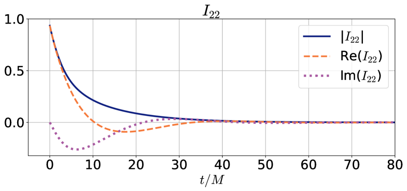
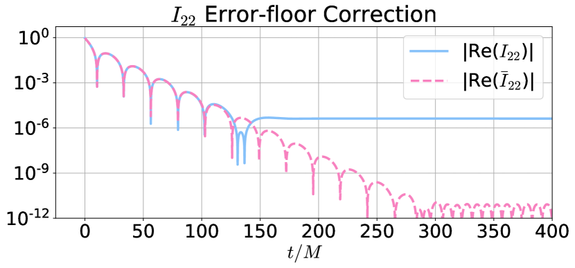
Figure 2: The mass moment $I_{22}$ and its floor correction. The top panel shows $|I_{22}|$ in blue/solid, Re($I_{22}$) in orange/dashed, and Im($I_{22}$) in purple/dotted. The bottom panel shows $|\mathrm{Re}(I_{22})|$ in cyan/solid. This curve directly demonstrates the damped oscillation pattern of $I_{22}$. It also reveals a numerical floor at the level $4\times 10^{-6}$ after $t\sim 150M$. Subtracting this floor from $I_{22}$, we obtain the floor-corrected mass moment $\bar{I}_{22}$, which is shown in pink/dashed in the bottom panel. The pattern of damped oscillation extends to $t\sim 280M$.

To further analyze the behavior of this mass moment, we will implement the rotation procedure outlined in Sec. III.2. We first check the validity of Eq. (54) in the simulation at late times by comparing $\Omega_{H}$ with $\Omega_{t}$. Here, $\Omega_{t}$ is defined as the average value of $X^{\grave{\phi}}$ (the $\grave{\phi}$-component of $X^{a}$) over the common horizon $\mathcal{S}$ at time $t$, i.e.,

$$\Omega_{t}=\underset{\mathcal{S}}{\text{mean}}\left(X^{\grave{\phi}}\right).$$ (56)

Note that in the simulation, the maximum deviation of $X^{\grave{\phi}}$ from $\Omega_{t}$ on every $\mathcal{S}$ is within $10^{-5}$ for $t\geq 300M$, as expected. What is unexpected is shown in the top panel of Fig. 3: Although we expect $\Omega_{t}$ to approach the horizon angular velocity [40],

$$\Omega_{H}=\frac{\chi_{f}}{2M_{f}\left(1+\sqrt{1-\chi_{f}^{2}}\right)}=0.208819M^{-1},$$ (57)

it does not completely settle down even at $t=t_{f}=500M$. Nevertheless, as $\Omega_{t}$ varies gradually near $t=500M$, we set the rotational frequency of the transformation $\phi\to\phi-\Omega t$ in this paper to be

$$\Omega=\Omega_{t=500M}=0.208784M^{-1}.$$ (58)

All results in the following sections are based on this choice. We also show the relative difference between $\Omega_{t}$ and $\Omega_{H}$ in the inset.

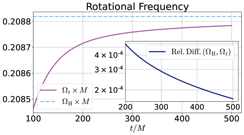
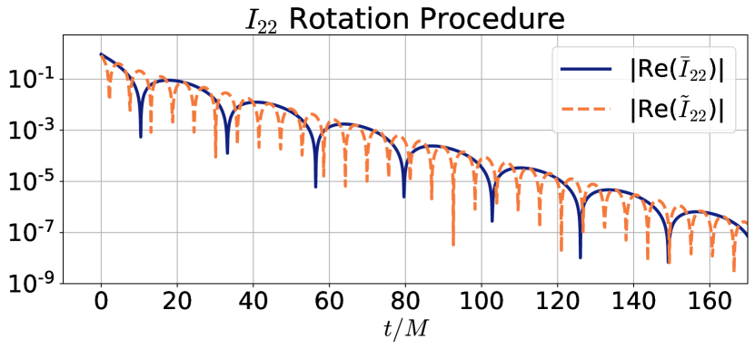
Figure 3: The rotational frequency of $Y_{\ell m}$ and the rotated mass moment. The top panel shows $\Omega_{t}$ (purple/solid), the rotational frequency of $Y_{\ell m}$, as a function of time. The curve does not settle down to a constant even at a very late time. This panel also shows $\Omega_{H}$ (cyan/dashed), the horizon angular velocity, as a reference. The relative difference between $\Omega_{t}$ and $\Omega_{H}$ is given in the inset. We show the comparison between $\bar{I}_{22}$ (blue/solid) and its rotated version $\tilde{I}_{22}$ (orange/dashed) in the bottom panel. Applying the rotation does not alter the decay rate, but it increases the frequency significantly.

We rotate the mass moments by defining

$$\tilde{I}_{\ell m}(t)=\bar{I}_{\ell m}(t)e^{-im\Omega t}.$$ (59)

The bottom panel of Fig. 3 compares the rotated mass moment $|\mathrm{Re}(\tilde{I}_{22})|$ (orange/dashed) with the nonrotated one $|\mathrm{Re}(\bar{I}_{22})|$ (blue/solid). The rotation does not change the decay rate of the mass moment but greatly increases its oscillation frequency: $\tilde{I}_{22}$ oscillates almost four times as quickly as $\bar{I}_{22}$. Thus, the use of $\bar{I}_{22}$ or $\tilde{I}_{22}$ may lead to very different conclusions. In this paper, we choose to investigate the behavior of $\tilde{I}_{22}$, namely the rotated, error-floor-corrected $(2,2)$ mass moment. As we will see, the behavior of this mass moment resembles that of a gravitational waveform.

Our first step in the analysis of $\tilde{I}_{22}$ is to compare it with the waveform strain $h$. We extract $h$ on the surfaces of multiple concentric spherical shells of finite Euclidean radii $r$, and extrapolate $rh$ to $\mathscr{I}^{+}$ as a function of retarded time $t_{\mathrm{ret}}$ [72, 73, 74, 75, 76]. Then, $rh_{22}$ is the $(\ell=2,m=2)$ coefficient in the $s=-2$ spin-weighted spherical harmonic expansion of $rh$. Note that $rh_{22}$ is both time shifted and phase shifted in this paper: We set $t_{\mathrm{ret}}=0$ when $|rh_{22}|$ (not necessarily $|rh|$) reaches its maximum. We also multiply $rh_{22}$ by a constant complex factor such that $rh_{22}(t_{\mathrm{ret}}=50M)$ matches $\tilde{I}_{22}(t=50M)$. We show both $\tilde{I}_{22}$ (blue/solid) and $rh_{22}$ (orange/dashed) in Fig. 4. The graph displays the absolute values of their real parts, so that we can compare the decay and oscillation between the two curves simultaneously. The horizontal axes represent the simulation time $t$ for $\tilde{I}_{22}$ and the retarded time $t_{\mathrm{ret}}$ for $rh_{22}$. We see from the graph that $\tilde{I}_{22}$ and $rh_{22}$ are strongly correlated. Specifically, in the range $20M\leq t\leq 120M$, they share the same decay constant and oscillation frequency. For $t>120M$ (not shown), the comparison becomes meaningless, because the strain reaches its level of numerical error. For $t<20M$, $\tilde{I}_{22}$ and $rh_{22}$ are less correlated, possibly because the meaning of time (or the behavior of the lapse) in the strong field regime is substantially different from at infinity.

Figure 4 strongly suggests that the mass moment $\tilde{I}_{22}$, like $h_{22}$, is described by the QNM of spin-weight $s=-2$ or $s=2$. We include the possibility $s=2$ here, because the frequency of an $s=2$ QNM is the same as that of $s=-2$. Knowing that $\tilde{I}_{22}$ has spin weight 0, one might be curious about why $\tilde{I}_{22}$ is described by $s=\pm 2$ QNMs. The expression of $\tilde{R}$’s first order perturbation, Eq. (2.21) in Hartle’s [77], provides a potential explanation.

In the following sections, we investigate the quasinormal pattern of $\tilde{I}_{22}$ quantitatively, by linearly fitting $\tilde{I}_{22}$ to multiple QNMs of spin weight $s=2$ (or equivalently $s=-2$).

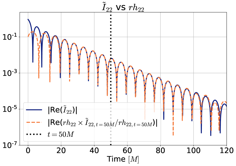
Figure 4: The comparison between the mass moment $\tilde{I}_{22}$ (blue/solid) and the waveform $rh_{22}$ (orange/dashed). The mass moment is plotted as a function of simulation time $t$, while the waveform is of retarded time $t_{\mathrm{ret}}$. The waveform is time shifted and multiplied by a constant factor, as described in the main text. The black dotted vertical line marks $t=50M$, at which the values of two curves are matched. We see strong correlation between these two quantities in $20M\leq t\leq 120M$.

IV.1.1 Mode mixing

We start with a model with only fundamental modes,

$$\tilde{I}_{22}=\sum_{\ell=2}^{L}C_{\ell 20}e^{-i\omega_{\ell 20}(t-t_{0})},$$ (60)

with a fitting time range $t_{0}\leq t\leq 120M$. We choose $120M$ as the end fitting time, when the mass moment is still slightly above the numerical error of $\tilde{I}_{22}$ (see Fig. 2). The parameters $C_{\ell 20}$ are to be determined by a linear fit. (All the symbols $C_{\ell mn}$ in this paper should be understood as fitting parameters.) We consider several $L\geq 2$ and allow $t_{0}$ to vary. We measure the error of fit by the mismatch between $\tilde{I}_{22}$ and its fit. The mismatch between two complex-valued functions $f(t)$ and $g(t)$ is defined as

$$\mathcal{M}(f,g)=1-\frac{\mathrm{Re}(\langle f|g\rangle)}{\sqrt{\langle f|f\rangle\langle g|g\rangle}},$$ (61)

where

$$\langle f|g\rangle=\int f(t)g^{*}(t)dt,$$ (62)

with integration domain over the fitting time range.

We first consider the simplest choice $L=2$ in this model, which means we fit $\tilde{I}_{22}$ using only the fundamental tone of $(2,2)$ QNMs. The mismatch $\mathcal{M}$ as a function of the initial fitting time $t_{0}$ is shown in blue (solid) in Fig. 5. The curve decays from $10^{-2}$ to $10^{-5}$ before $t_{0}=18M$. This decay is expected, because the current model does not include overtones, which are strongly excited near the merger. However, it is surprising to see a wavy pattern in the curve after $t_{0}=18M$, since the QNM fit of $rh_{22}$ does not have such a feature [19, 54]. This oscillatory pattern extends well beyond $t_{0}=70M$, which is not shown.

This oscillatory pattern suggests that the $L=2$ model does not capture an essential feature of $\tilde{I}_{22}$. We can rule out the following two possibilities for this missing feature. First, this feature is not related to the oscillation of $\bar{I}_{22}$, i.e., the nonrotated mass moment. This is because the period of the oscillatory pattern in the $L=2$ mismatch curve ($\sim$$26M$) differs from the period of $\bar{I}_{22}$. Second, the missing feature is not related to the $\omega_{22n}$ overtones either, because the oscillatory pattern cannot be eliminated by including them in the $L=2$ model (not shown). Accordingly, we consider one more possibility: There is another fundamental tone, other than $\omega_{220}$, that contributes to $\tilde{I}_{22}$. Indeed, $\omega_{220}$ and $\omega_{320}$ share a similar decay rate, and they can generate a beat period of $26.3M$ (see Table 2), which is close to the period of the oscillatory pattern ($\sim$$26M$). So we now examine the model Eq. (60) with $L=3$. The orange dashed curve in Fig. 5 represents the mismatch using this model. It contains no oscillatory pattern at late times, confirming the nonnegligible contribution of the $(3,2)$ fundamental tone to $\tilde{I}_{22}$. The curve decreases steadily after the local maximum at $t=27.4M$, so we may treat $t=27.4M$ as the instant when overtones are negligible, and only two fundamental tones dominate. We have also investigated the $L=4$ and $L=5$ cases, but they hardly improve the fit (not shown).

We now connect the presence of the $(3,2)$ QNM in the description of $\tilde{I}_{22}$ to the concept of mode mixing. In BH perturbation theory, the natural angular basis for strain $h$ (whose second time derivative is $\Psi_{4}$) is the spin-weighted spheroidal harmonics (Sec. II.3). However, the natural angular basis for $h$ at future null infinity $\mathcal{I}^{+}$ is the basis of the spin-weighted spherical harmonics [69]. This is the basis used, for example, in LIGO waveform analysis. The use of spherical harmonics intertwines spheroidal modes of the same $m$ but different $\ell$ [78]. For example, the spherical mode $h_{22}$ (i.e., the expansion coefficient corresponding to ${}_{-2}Y_{22}$) can be decomposed into not only the $\omega_{22n}$ modes, but also the $\omega_{32n}$ modes, etc. This phenomenon is called mode mixing. In our BBH configuration (equal-mass, non-spinning), modes other than $\omega_{22n}$ may be ignored in $h_{22}$’s decomposition. This is because the $\omega_{22n}$ modes are strongly dominant [18], and the mixing of spheroidal and spherical harmonics is tiny [78]. However, this argument does not apply to mass moments $I_{\ell m}$. The natural angular basis of the perturbed $\tilde{\mathcal{R}}$ in Eq. (31) is neither spheroidal nor spherical harmonics, but a complicated function of angles $(\theta,\phi)$ instead. The mixing of this complicated angular function and spherical harmonics, if nonnegligible, would lead to the presence of $(3,2)$ QNMs in $\tilde{I}_{22}$. In this paper, we refer to this phenomenon as mode mixing as well, but in a somewhat broader sense.

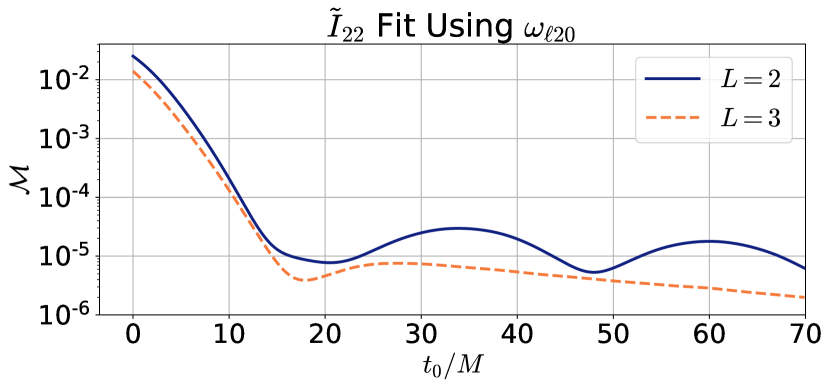
Figure 5: The mismatch between $\tilde{I}_{22}$ and its fit using $\omega_{\ell 20}$ QNMs [Eq. (60)], plotted as a function of the initial fitting time $t_{0}$. Both the $L=2$ (blue/solid) and $L=3$ (orange/dashed) curves decay sharply before $t_{0}=18M$, because overtones are not included in the model. The $L=2$ curve, which only uses the $\omega_{220}$ QNM, contains a persistent oscillatory pattern after $t_{0}=18M$. This is a beat pattern formed by the $\omega_{220}$ and $\omega_{320}$ QNMs, and is removed in the $L=3$ curve.

Now that we know $\tilde{I}_{22}$ can be well approximated by the fundamental tones of $(2,2)$ and $(3,2)$ QNMs after $t=27.4M$, we shall analyze the effect of overtones on $\tilde{I}_{22}$. Inspired by the use of overtones in the QNM fit of waveforms and horizon moments in Refs. [19, 54, 22], we consider the following model,

$$\tilde{I}_{22}=C_{320}e^{-i\omega_{320}(t-t_{0})}+\sum_{n=0}^{N}C_{22n}e^{-i\omega_{22n}(t-t_{0})},$$ (63)

with the same fitting time range $t_{0}\leq t\leq 120M$. Figure 6 shows the mismatch of this model as a function of $t_{0}$ for multiple $N$ ($0\leq N\leq 3$). By construction, the $N=0$ curve is the same as the $L=3$ curve in Fig. 5. As more overtones are included, the mismatch curve becomes flatter and lower, and the initial damping part shrinks and ends earlier. For $N=3$, we no longer see the initial damping part. This means that the overtones $\omega_{22n}$ (at least for $1\leq n\leq 3$) do contribute to $\tilde{I}_{22}$, and the fitting model Eq. (63) indeed captures them. Note that compared to the $N=0$ model, those $N\geq 1$ models improve the accuracy even after the overtones are supposed to damp away. This might be caused by overfitting to numerical noise. We also checked several $N\geq 4$ models, but they do not display much improvement (not shown) compared to the $N=3$ model.

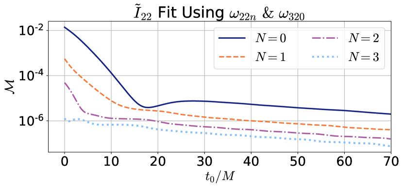
Figure 6: The mismatch between $\tilde{I}_{22}$ and its fit using $\omega_{22n}$ and $\omega_{320}$ QNMs [Eq. (63)]. The $N=0$ curve is, by construction, the same as the $L=3$ curve in Fig. 5. Adding higher overtones renders a better fit for all $t_{0}$, and specifically, brings down the portion of large mismatch before $t\sim 10M$. This figure demonstrates the important contribution of overtones to the mass moment.

IV.1.2 Fit using fundamental tones

In this section, we will have a closer look at the late-time QNM description of $\tilde{I}_{22}$. We continue using the model Eq. (60) with $L=3$, which reads

$$\tilde{I}_{22}=C_{220}e^{-i\omega_{220}(t-t_{0})}+C_{320}e^{-i\omega_{320}(t-t_{0})}.$$ (64)

Instead of varying $t_{0}$ as in the previous section, we now fix the value of $t_{0}$. In particular, we choose $t_{0}=50M$, at which all overtones have decayed sufficiently.

The top left panel of Fig. 7 shows the fit using this model with the fitting time range $50M\leq t\leq 120M$. The blue solid curve represents the actual mass moment $\tilde{I}_{22}$, while the orange dashed curve represents the fit. They are both plotted in the magnitude of their real parts. We see that the two curves overlap very well, so the model Eq. (64) indeed provides a good description of $\tilde{I}_{22}$. The relative difference between $\tilde{I}_{22}$ and its fit (including their imaginary parts) is plotted in purple (solid) in the bottom panel of the same figure. For reference, the cyan dashed curve in this panel is the relative difference in $\tilde{I}_{22}$ between the two resolutions used in our simulation (Sec. III.1), which provides another estimate of the numerical error of $\tilde{I}_{22}$. Note that both curves in the bottom panel have an increasing trend, as $\tilde{I}_{22}$ gets closer to the level of numerical uncertainty. After $t\geq 80M$, the relative error of the QNM fit is larger than the numerical error of $\tilde{I}_{22}$ by about two orders of magnitude. This means the model is good but not perfect, and there is room for improvement in the future.

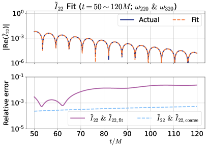
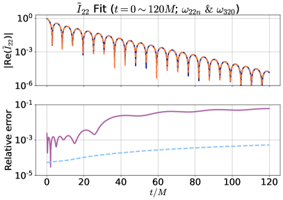
Figure 7: The comparison between $\tilde{I}_{22}$ and its fit. The left two panels are based on the fit using $\omega_{220}$ and $\omega_{320}$ [Eq. (64)], in the time range $50M\leq t\leq 120M$. The right two panels are based on the fit using {$\omega_{220}$, $\omega_{221}$, $\omega_{222}$, $\omega_{223}$, $\omega_{320}$} [Eq. (63) with $N=3$], in the time range $0\leq t\leq 120M$. The top two panels show the absolute real parts of $\tilde{I}_{22}$ (blue/solid) and its fit (orange/dashed). In either top panel, the two curves overlap very well. The bottom two panels show the relative difference between $\tilde{I}_{22}$ and the fit in purple/solid, and the difference in $\tilde{I}_{22}$ between two resolutions in cyan/dashed. The quantity $\tilde{I}_{22,\mathrm{coarse}}$ refers to the $(2,2)$ mass moment extracted from the low-resolution simulation.

Once we accept that the model Eq. (64) can describe the mass moment at late times, we may use it to estimate the final mass and spin of the remnant. The QNM frequencies $\omega_{220}$ and $\omega_{320}$ used to generate the left panels of Fig. 7 are calculated based on $M_{f}$ and $\chi_{f}$ that are measured by SpEC (Sec. III.1). In the following discussion, we regard the SpEC values of $M_{f}$ and $\chi_{f}$ as their true values. Now, we allow $M_{f}$ and $\chi_{f}$ to deviate from the true values, and repeat the QNM fit over the ($M_{f},\chi_{f}$) parameter space (similar to the procedure in Ref. [19]). For each ($M_{f},\chi_{f}$) combination, we measure the error of the fit by the mismatch, Eq. (61). The result is visualized as a heat map of $\log_{10}\mathcal{M}$ in the left panel of Fig. 8: the lighter the shading, the smaller the mismatch. We also show the true values of $M_{f}$ and $\chi_{f}$ in golden (solid) lines for reference. We see from the plot that not only does the mismatch have a deep minimum over the ($M_{f},\chi_{f}$) parameter space, but also the minimum approximately recovers the true values. In particular, the best estimates of the mass and spin (i.e., their values at the minimum) are $M_{f}^{\prime}=0.95390M$ and $\chi_{f}^{\prime}=0.68825$. We can assess the goodness of these estimates by the error,

$$\epsilon_{f}=\sqrt{(M_{f}^{\prime}-M_{f})^{2}/M^{2}+(\chi_{f}^{\prime}-\chi_{f})^{2}},$$ (65)

as proposed in Ref. [19]. The error of these estimates is $\epsilon_{f}=2.9\times 10^{-3}$, compared to a difference between the two resolutions, $3\times 10^{-6}$. Note that the minimum mismatch does not necessarily make ($M_{f}^{\prime}$, $\chi_{f}^{\prime}$) a better pair of candidates for the final mass and spin, because as we will see, different QNM models produce different ($M_{f}^{\prime},\chi_{f}^{\prime}$) combinations, and there is no consistent choice among these models to determine mass and spin yet.

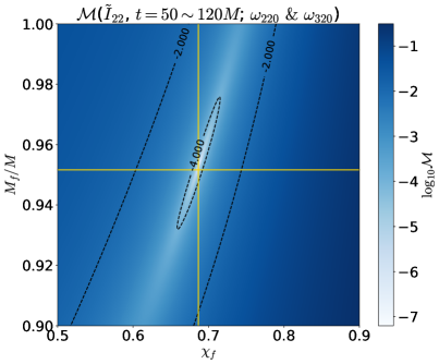
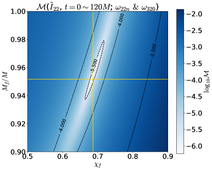
Figure 8: Heat maps of the mismatch $\log_{10}\mathcal{M}$ over the ($M_{f},\chi_{f}$) parameter space. The left panel is based on the model Eq. (64), while the right one on the model Eq. (63) with $N=3$: the lighter the shading, the smaller the mismatch. In each panel, we use two golden lines to represent the true values of $M_{f}$ and $\chi_{f}$. The dashed curves are the contour lines of constant mismatch. The deep minimum of the mismatch is located close to the golden cross, which means that the QNM model can be used to recover the true values of the remnant parameters.

IV.1.3 Fit using overtones

We extend the analysis in the previous section to the early-time portion of $\tilde{I}_{22}$, by including overtones up to $n=3$. In particular, we investigate the model Eq. (63) with $N=3$, and fix the fitting time range as $0\leq t\leq 120M$. The right panels of Fig. 7 shows the comparison between the actual $\tilde{I}_{22}$ and its QNM fit using this $N=3$ model. We see from the top panel that the QNM description of the $(2,2)$ mass moment is valid even near the merger. The relative error of this fit is $10^{-3}$ – $10^{-2}$, which is about two orders of magnitude greater than the numerical error measured by the difference in $\tilde{I}_{22}$ between two resolutions, as shown in the bottom panel. Again, this means the model could be improved in the future.

This model also provides an estimate of the final mass and spin of the remnant. The right panel of Fig. 8 shows the mismatch heat map over the ($M_{f},\chi_{f}$) parameter space, together with a golden cross representing the true $M_{f}$ and $\chi_{f}$. Once more, we see a deep minimum near the golden cross. The mass ($M_{f}^{\prime}=0.95699M$) and spin ($\chi_{f}^{\prime}=0.69066$) at the minimum reproduce the true values, with error $\epsilon_{f}=6.8\times 10^{-3}$. This result also rules out overfitting partially, because almost any ($M_{f},\chi_{f}$) combination yields a worse fit than the true values. We cannot completely rule out overfitting since the five complex frequencies represent 10 real degrees of freedom, and we only vary two (final mass and spin).

IV.2 ($\mathbf{3,2}$) spin moment

The $(3,2)$ spin moment $L_{32}$ is the dominant mode among $L_{\ell m}$ with nonzero $m$. Figure 9 shows the value of $|\mathrm{Re}(L_{32})|$, i.e., the magnitude of the real part of $L_{32}$, in cyan (solid). Similar to the $|\mathrm{Re}(I_{22})|$ curve in Fig. 2, this curve has a pattern of damped oscillation before $t=150M$, and then stays unchanged on a $5\times 10^{-6}$ numerical error floor after $t=150M$. We subtract this floor from $L_{32}$ and define the floor-corrected spin moment

$$\bar{L}_{32}=L_{32}-\mathrm{mean}[L_{32}(t\geq 400M)].$$ (66)

The pink dashed curve in Fig. 9 represents the value of $|\mathrm{Re}(\bar{L}_{32})|$. After the error floor correction, the damped oscillation extends to $t=280M$. Nevertheless, we will only focus on the portion $t\leq 150M$ of $\bar{L}_{32}$ henceforth. In Fig. 9, we also observe that the early-time portion of both curves does not follow a normal damped-oscillatory pattern: the first 3 – 4 cycles are stretched wider at the local maxima, especially near $t\sim 25M$ and $t\sim 50M$. This is caused by mode mixing, as we shall see in the following subsection. This feature is not visible in Fig. 2, where the mixing of modes is relatively small.

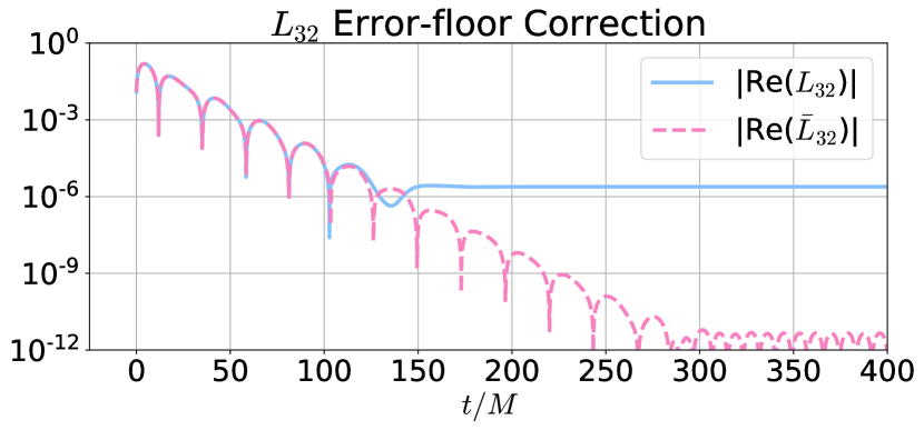
Figure 9: The spin moment $L_{32}$ and its floor correction. The original $(3,2)$ spin moment (cyan/solid) reaches a numerical floor at the level $5\times 10^{-6}$ after $t\sim 150M$. We define the floor-corrected spin moment $\bar{L}_{32}$ (pink/dashed) by subtracting the floor from $L_{32}$. The damped oscillatory pattern of $\bar{L}_{32}$ extends to $t\sim 280M$. We also observe that the first several cycles are stretched wider near the local maxima.

IV.2.1 Mode mixing

Following the rotation procedure in Sec. III.2, we define the rotated spin moments,

$$\tilde{L}_{\ell m}(t)=\bar{L}_{\ell m}(t)e^{-im\Omega t},$$ (67)

and investigate the mode mixing in $\tilde{L}_{32}$. We perform a QNM fit of $\tilde{L}_{32}$ using the following model:

$$\tilde{L}_{32}=\sum_{\ell\in Q}C_{\ell 20}e^{-i\omega_{\ell 20}(t-t_{0})}.$$ (68)

We choose the fitting time range to be $t_{0}\leq t\leq 120M$, with $t_{0}$ varying, and assess the goodness of fit by mismatch [Eq. (61)]. The set $Q$ consists of integers to be specified. Since we are investigating the $(\ell=3,m=2)$ spin moment, the most intuitive choice of $Q$ is the singleton {3}, i.e., only considering the $(3,2)$ QNM. However, this choice completely fails the QNM fit with mismatch always above 0.1, as indicated by the blue solid curve in Fig. 10. The best single-$\ell$ model is actually of $\ell=2$ (the orange dashed curve in the same graph), whose mismatch is smaller than the $\ell=3$ curve (blue/dashed) by a factor of 10 after $t_{0}=10M$. Thus, the $(2,2)$ QNM is the actual dominant mode in $\tilde{L}_{32}$. This is not unreasonable, because the perturbation of $\tilde{D}_{a}(\tilde{\epsilon}^{ab}\omega_{b})$ [see $L_{\ell m}$’s definition, Eq. (32)] is not guaranteed to satisfy the Teukolsky equation.

From Fig. 10, we see that even the best single-$\ell$ model has poor performance with mismatch $\sim$$10^{-2}$. Thus, we move on to models using two different $\ell$’s. In particular, we consider all possible pairs of $\ell$ among $\{2,3,4,5\}$. The pair $\ell=2,3$ yields the best QNM fit, as shown in purple/dash-dot in Fig. 10, while all other pairs produce much worse mismatch (not shown). The mismatch of the $\ell=2,3$ curve is much smaller than the $\ell=2$ curve (orange/dashed), by a factor of $\sim$1000 after $t=20M$. This means that the $(2,2)$ and $(3,2)$ QNMs are the first two dominant modes in $\tilde{L}_{32}$. It also demonstrates that a two-$\ell$ model can outperform any single-$\ell$ model when mode mixing is significant.

The purple dash-dot curve in Fig. 10 has a wavy pattern after $t=20M$, similar to the $L=2$ curve in Fig. 5, which suggests a further mode mixing. This oscillatory feature is indeed reduced by using the $\ell=2,3,4$ model, as shown by the cyan dotted curve in Fig. 10. We continued expanding the model to include more $\ell$, but we found the improvement negligible (not shown). Hence, our $(3,2)$ spin moment is best described by a linear combination of the $(2,2)$, $(3,2)$ and $(4,2)$ QNMs at late times ($t\geq 20M$).

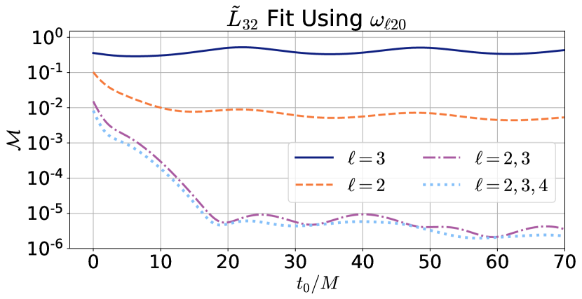
Figure 10: The mismatch between $\tilde{L}_{32}$ and its fit using the model Eq. (68). The intuitive choice $Q=\{3\}$ (blue/solid) actually produces the QNM fit with the largest mismatch. The best single-$\ell$ model uses $\ell=2$ (orange/dashed), producing a mismatch $\sim$$10^{-2}$. The best two-$\ell$ model uses $\ell=2,3$ (purple/dash-dot), which decreases the mismatch by a factor of $\sim$1000 compared to the orange dashed curve after $t_{0}=20M$. The $\ell=2,3$ curve exhibits a wavy pattern, which can be reduced by using the $\ell=2,3,4$ model (cyan/dotted).

For $t\leq 20M$, the mismatch of the $\ell=2,3,4$ model (cyan/dotted) decays sharply from $10^{-2}$ to $10^{-5}$. To probe the effect of overtones on the early-time behavior of $\tilde{L}_{32}$, we consider the following fitting model,

$$\tilde{L}_{32} =C_{320}e^{-i\omega_{320}(t-t_{0})}+C_{420}e^{-i\omega_{420}(t-t_{0})}$$

$$+\sum_{n=0}^{N}C_{22n}e^{-i\omega_{22n}(t-t_{0})},$$ (69)

with the fitting range $t_{0}\leq t\leq 120M$. We plot the mismatch as a function of $t_{0}$ in Fig. 11 for five different $N$. By construction, the $N=0$ curve (blue/solid) is identical to the cyan dotted curve in Fig. 10. As more overtones are included, the mismatch decreases, and the initial decay pattern fades. However, it is yet unclear whether the decay completely disappears, because a newly emerging wavy pattern overshadows this decay. The wavy pattern is manifest in all four $N>0$ curves and persists for even higher $N$ (not shown). This suggests more potential mixing from other QNMs, which we do not pursue further in this paper.

Figure 11: The mismatch between $\tilde{L}_{32}$ and its fit using the model Eq. (69). By construction, the $N=0$ curve is the same as the cyan dotted curve in Fig. 10. Including higher overtones brings down the mismatch, but also reveals a new oscillatory pattern. Unless this pattern is resolved, the effect of overtones on $\tilde{L}_{32}$ remains unclear.

IV.3 ($\mathbf{2,0}$) mass moment

There are two major differences between multipole moments of $m=0$ and those of $m\neq 0$. First, an $m=0$ multipole moment is real-valued, while an $m\neq 0$ mode is complex-valued. Second, as the remnant BH settles down, a nontrivial $m=0$ mode tends to a nonzero constant, while a nontrivial $m\neq 0$ mode always tends to 0. Because of these distinctions, it is instructive to discuss $m=0$ multipole moments separately. We apply the techniques used in the previous two sections (Secs. IV.1 and IV.2) on $I_{20}$, but with slight modification.

Mass and spin moments of a Kerr BH can be calculated theoretically given its mass and spin [8]. Let $I_{20,\mathrm{theory}}$ be the theoretical value of the $(2,0)$ mass moment of a Kerr BH. We find that the relative difference between $I_{20}$ and $I_{20,\mathrm{theory}}$ always lies below $4\times 10^{-6}$ after $t=150M$, so our $I_{20}$ indeed approaches the expected value. To investigate the possible QNM description of $I_{20}$, we subtract its asymptotic value and define

$$\bar{I}_{20}=I_{20}-\mathrm{mean}[I_{20}(t\geq 400M)].$$ (70)

This is similar to Eq. (55), except that the nonzero value of $I_{20}$ at a late time is related to the horizon geometry instead of numerical errors. Note that for $m=0$, there is no need to rotate $\bar{I}_{20}$, and we can directly set $\tilde{I}_{20}=\bar{I}_{20}$ [see Eq. (59)].

We expect $\tilde{I}_{20}$ to be described by the fundamental tone of the $(2,0)$ QNM at late times. Because $\omega_{200}$ is a complex number while $\tilde{I}_{20}$ is real-valued, we use the following fitting model for $\tilde{I}_{20}$,

$$\tilde{I}_{20}=e^{-\lambda_{1}(t-t_{0})}[A_{1}\cos\lambda_{2}(t-t_{0})+A_{2}\sin\lambda_{2}(t-t_{0})],$$ (71)

where $\lambda_{1}$ and $\lambda_{2}$ are the real and imaginary parts of $-\omega_{200}$. The real parameters $A_{1}$ and $A_{2}$ are to be determined by a linear fit. The fitting range is $t_{0}\leq t\leq 120M$ as usual. We first vary $t_{0}$ and analyze the mismatch Eq. (61) as a function of $t_{0}$ in Fig. 12. This curve ultimately reaches the level of $10^{-5}$, but very gradually. This is different from the mismatch curve of $\tilde{I}_{22}$ fit by the $\omega_{220}$ mode (the blue solid curve in Fig. 5), which damps sharply to the $10^{-5}$ level before $t_{0}=20M$. Such a distinction is unexpected, because the decay rates of $\omega_{200}$ and $\omega_{220}$ differ by only a few percent (see Table 2). This suggests that the model Eq. (71) may not be appropriate for $\tilde{I}_{20}$ before $t_{0}=70M$ (at which $\tilde{I}_{20}$ drops to near $10^{-5}$).

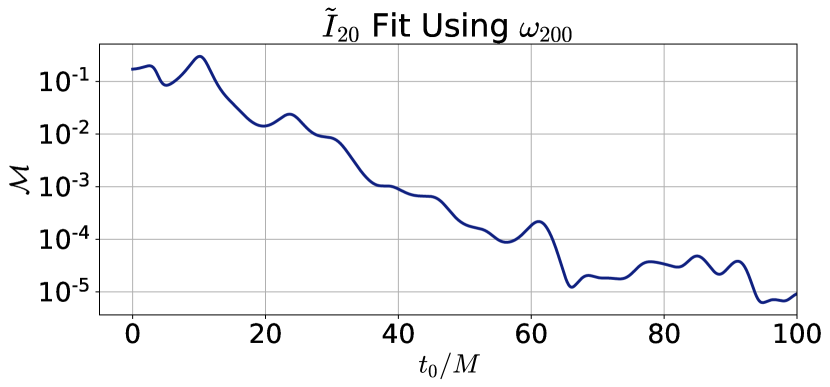
Figure 12: The mismatch between $\tilde{I}_{20}$ and its fit using the $\omega_{200}$ QNM [Eq. (71)]. The mismatch decays to the $10^{-5}$ level very slowly, unlike the $\tilde{I}_{22}$ case. There are irregular bumps along the curve, which is in stark contrast to the smooth curves in Figs. 7 and 10. The origin of these bumps is unknown.

Next, we examine the performance of the model after $t=70M$, by fitting $\tilde{I}_{20}$ with the $\omega_{200}$ mode in the time range $70M\leq t\leq 120M$. The top panel of Fig. 13 displays both $\tilde{I}_{20}$ and its fit, which overlap to within about 1% relative error. The absolute difference between these two curves is shown in purple (solid) in the bottom panel. Here, we use the absolute difference instead of relative difference to measure error, because $\tilde{I}_{20}$ crosses zero periodically. The amplitude of the purple solid curve stays near the level $10^{-7}$, which means the relative error is at the level $10^{-2}$ – $10^{-1}$, after we take into account the magnitude of $\tilde{I}_{20}$. The bottom panel also shows the absolute difference in $\tilde{I}_{20}$ between two resolutions for reference (cyan/dashed). The figure indicates that $\tilde{I}_{20}$ can be reasonably described by the $\omega_{200}$ mode at sufficiently late times.

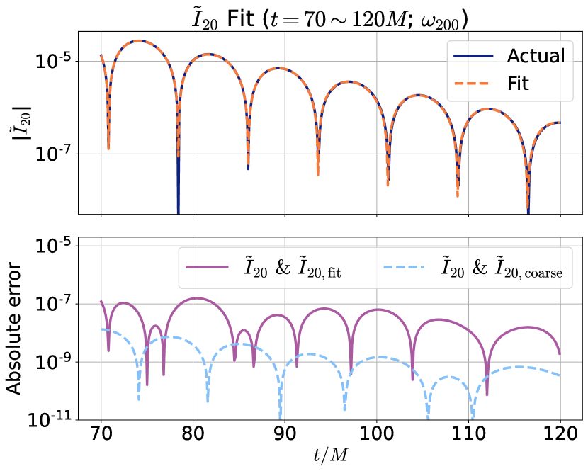
Figure 13: The comparison between $\tilde{I}_{20}$ and its fit based on the model Eq. (71). The top panel shows the absolute values of $\tilde{I}_{20}$ (blue/solid) and the fit (orange/dashed), and these two curves overlap well. The bottom panel shows the absolute difference between $\tilde{I}_{20}$ and the fit in purple/solid, and the difference in $\tilde{I}_{20}$ between two resolution in cyan/dashed.

Knowing that the model Eq. (71) can describe the late-time behavior of $\tilde{I}_{20}$, we would like to estimate the final mass and spin by minimizing the mismatch of the fit. The outcome is not so satisfactory compared to the previous cases. Figure 14 shows the mismatch of the QNM fit (with the fitting range $70M\leq t\leq 120M$), as both the final mass and spin vary. Again, the golden lines represent the true mass and spin, and a lighter-shaded region has lower mismatch. The local minimum is achieved at $M_{f}^{\prime}=0.95374M$ and $\chi_{f}^{\prime}=0.69868$, which yields an error $\epsilon_{f}=1.2\times 10^{-2}$, about 4 times the error $\epsilon_{f}$ in Sec. IV.1.2. This means that, with regard to the performance of mass or spin estimate, fitting $\tilde{I}_{20}$ is inferior to fitting $\tilde{I}_{22}$. To understand why the $\omega_{200}$ model for $\tilde{I}_{20}$ is less faithful, we should realize that this model is not very sensitive to the remnant parameters. This can be seen from Fig. 14, where the local minimum of the mismatch is shallow. Specifically, the minimum mismatch is $1.61\times 10^{-5}$, which is very close to the mismatch at the true mass and spin, $1.87\times 10^{-5}$. There is actually a fundamental reason for the weakness of this model: the variation in the values of $\omega_{200}$ versus spin is much smaller than the one of $\omega_{220}$. In particular, as the spin ranges from 0.5 to 0.9, Re($\omega_{220}$) increases by 45%, while Re($\omega_{200}$) by only 7%. In summary, the $\omega_{200}$ model is a reasonable but spin-insensitive model for $\tilde{I}_{20}$ at late times.

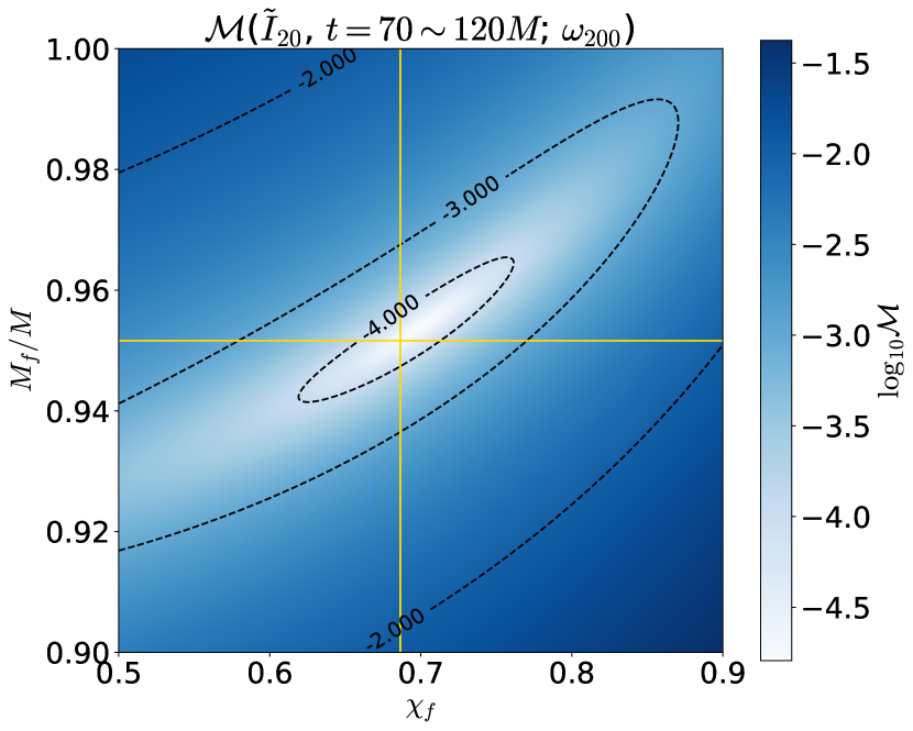
Figure 14: Heat map of the mismatch $\log_{10}\mathcal{M}$ over the ($M_{f},\chi_{f}$) parameter space. This is generated based on the fit of $\tilde{I}_{20}$ using the model Eq. (71). The fitting time range is $70M<t<120M$. The color representation is similar to Fig. 8, and we again use two golden lines to represent the true values. The dashed curves are the contour lines of constant mismatch. Although the minimum mismatch is located near the golden cross, the minimum is shallow, as discussed in Sec. IV.3.

IV.4 Other multipole moments

Here, we briefly summarize the results for those multipole moments that have not been discussed previously. We will focus on the nontrivial $\tilde{I}_{\ell m}$ and $\tilde{L}_{\ell m}$ up to $\ell=6$. Note that these multipole moments are all floor-corrected and rotated.

We start with the multipole moments with $\ell=m$, specifically, $\tilde{I}_{44}$ and $\tilde{I}_{66}$. Fitting $\tilde{I}_{44}$ or $\tilde{I}_{66}$ with a single-$\ell$ QNM model results in a beat pattern at late times, so there is mode mixing in both cases. The best multi-$\ell$ model (with $m$ fixed) for the late-time behavior of $\tilde{I}_{44}$ consists of the $\omega_{440}$ and $\omega_{540}$ modes, while the best model for $\tilde{I}_{66}$ consists of $\omega_{660}$ and $\omega_{760}$. We have not found any good model that describes the early-time behavior of $\tilde{I}_{44}$ and $\tilde{I}_{66}$. For example, simply including $\omega_{44n}$ (or $\omega_{66n}$) overtones in a QNM model does not eliminate the initial decay of $\tilde{I}_{44}$ (or $\tilde{I}_{66}$).

Next, we consider the nontrivial multipole moments with $0<m<\ell$: $\tilde{I}_{42}$, $\tilde{I}_{62}$, $\tilde{I}_{64}$, $\tilde{L}_{52}$, and $\tilde{L}_{54}$. Their behaviors are very similar to that of $\tilde{L}_{32}$. Mode mixing is significant for these multipole moments, and the best multi-$\ell$ models for them are comprised of three or four fundamental tones of different $\ell$. For example, $\tilde{I}_{42}$, $\tilde{I}_{62}$, and $\tilde{L}_{52}$ are all best described by the {$\omega_{220}$, $\omega_{320}$, $\omega_{420}$, $\omega_{520}$} model at late times. For early-time behavior, adding overtones does greatly reduce the initial decay pattern, but this comes with the emergence of additional oscillatory patterns whose origin is unclear at this time.

Finally, we study the multipole moments with $m=0$: $\tilde{I}_{40}$, $\tilde{I}_{60}$, $\tilde{L}_{30}$, and $\tilde{L}_{50}$. They all approach their respective theoretical values with error below $1.2\times 10^{-5}$. The best multi-$\ell$ model [by extending Eq. (71)] for $\tilde{L}_{30}$ uses {$\omega_{200}$, $\omega_{300}$}, while the best model for $\tilde{I}_{40}$, $\tilde{L}_{50}$, and $\tilde{I}_{60}$ uses {$\omega_{200}$, $\omega_{300}$, $\omega_{400}$}. A common feature shared by these models is their failure to describe the multipole moments before $t\sim 60$ – $80M$. At sufficiently late times, these models do produce a good description of the respective multipole moments. However, we should keep in mind that the $m=0$ QNMs used in these models are not as sensitive to the remnant spin as the $m\neq 0$ QNMs, so the models might not be very precise.

V Conclusion

In this paper, we numerically construct the multipole moments on the common horizon of an equal-mass BBH system on a sequence of time slices. The construction process captures the connection among the common horizons on different time slices, which ensures that this set of multipole moments is spatially gauge independent. We apply a geometrically motivated rotation to the multipole moments, which turns out to simplify the analysis. We compare the multipole moments of the horizons with those of the gravitational waveform, and see a strong correlation between the $(\ell=2,m=2)$ mass multipole moment and the strain $(2,2)$-mode. Specifically, they share the same oscillation frequency and decay constant at late times. This suggests the possible QNM description of horizon multipole moments, which we pursue next.

We consider all nontrivial multipole moments up to $\ell=6$, and model each multipole moment as a linear combination of spin-weight-2 QNMs. At sufficiently late times, these multipole moments are well described by the fundamental tones of QNMs: not only do the true values overlap with the predicted values fit to the QNM models, but also the mismatch between them is small. However, the multipole moments do not match one-to-one with the fundamental tones, and we actually see a manifest mode-mixing phenomenon in all the multipole moments. For example, our best QNM model for the late-time behavior of the $(2,2)$ mass moment consists of the $\omega_{220}$ and $\omega_{320}$ QNMs, where the $\omega_{320}$ mode has a tiny but nonnegligible contribution. A more counter-intuitive example is the $(3,2)$ spin moment, in which the $\omega_{220}$ mode dominates over the $\omega_{320}$ mode, instead of vice versa. We find that in general, the $(\ell,m)$ multipole moment at late times is described by a QNM model consisting of the $(\ell^{\prime},m)$ fundamental tones for the first several possible $\ell^{\prime}$.

We also explore the possibility of QNM modeling for the early-time behavior of multipole moments by including overtones. We find that the inclusion of $\omega_{22n}$ overtones up to $n=3$ is sufficient to provide an accurate representation of the $(2,2)$ mass moment immediately after the merger. This extends the power of BH perturbation theory back to the time of coalescence. However, this picture does not apply to other multipole moments: a QNM model with overtones does reduce the mismatch significantly, but at the same time, it also unveils further mixing of modes. As a consequence, a more careful modeling with overtones is needed in the future to describe the early-time behavior of multipole moments other than the $(2,2)$ mass moment.

Taking into account the effect of mode mixing, we find that the QNM models using fundamental tones at late times provide a fairly faithful estimate of the remnant mass and spin, especially for those multipole moments of nonzero $m$. Furthermore, in the case of the $(2,2)$ mass moment, the QNM model with overtones also recovers the true mass and spin at the minimum mismatch. We also note that for the $m=0$ multipole moments, the performance of these estimates is not as good as in the $m\neq 0$ cases. This is interpreted as resulting from the weaker dependence of the $m=0$ mode frequencies on the spin.

In summary, this paper provides promising evidence for the QNM description of horizon multipole moments of a remnant BH in the ringdown phase of an equal-mass non-spinning BBH system. These multipole moments are spatially gauge independent, as we take into account the relation among apparent horizons in the construction step. Such gauge independence, along with the accuracy of the SpEC code, allows these multipole moments to be described with QNMs much more accurately than those horizon multipole moments constructed in previous literature (e.g., [8, 9]).

As future work, one can consider more generic BBH systems whose progenitors have different masses or nonzero spins, and then construct horizon multipole moments as outlined in this paper. One may also define a similar set of horizon multipole moments for the progenitor BHs, and investigate their possible imprint on the common horizon multipole moments. Note that Ref. [9] discusses the multipole moments of the progenitors, but the construction there does not yet capture the connection among the apparent horizons. Regarding the QNM models, one can continue improving them to mitigate the effect of mode mixing. Such improvement should reveal a clearer pattern in the early-time portion of horizon multipole moments.

Appendix A Balance laws and error convergence

As mentioned in Sec. II.2.4, the balance laws, Eqs. (44), (47), and (48), provide internal consistency checks for BH simulations. In this section, we use them to test the correctness of the BBH simulation in Sec. III.1. We start by showing the energy flux rate $d\mathcal{F}_{g}/dt$ in Fig. 15, as it is relevant to the area balance law. The graph displays the $\sigma$-part ($d\mathcal{F}_{g,\sigma}/dt$) in blue (solid) and the $\zeta$-part ($d\mathcal{F}_{g,\zeta}/dt$) in orange (dashed), as a function of simulation time $t$. We only show the time range $t\leq 30.8M$, since the calculation of the $\zeta$-part is numerically unstable at late times because of the divergence of the components of $\hat{r}^{a}$. Both curves decay exponentially, with higher decay rates near the merger. We see that the $\sigma$-part always dominates the $\zeta$-part, except at the merger. They differ by a factor of 2 – 3 after $t=5M$, which is not significant.

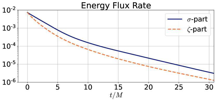
Figure 15: The energy flux rate $d\mathcal{F}_{g}/dt$. The rate consists of two parts, and we show the $\sigma$-part ($d\mathcal{F}_{g,\sigma}/dt$) in blue/solid and the $\zeta$-part ($d\mathcal{F}_{g,\zeta}/dt$) in orange/dashed. We only consider the time range $0\leq t\leq 30.8M$. Except at the merger, the $\sigma$-part is always greater than the $\zeta$-part, but the difference is not substantial: the $\sigma$-part is at most 2 – 3 times as much as the $\zeta$-part.

Next, we investigate the numerical violations of these three balance laws as functions of simulation time ($t\leq 30.8M$). The violations are measured by the relative difference between the left- and right-hand sides of their respective equations. We find that the area balance law [Eq. (44)] always holds within $10^{-4}$, and for most of the time within $10^{-5}$. The mass moment balance law [Eq. (47)] always holds within $3\times 10^{-6}$ for all nontrivial mass moments with $1\leq\ell\leq 8$, and the spin moment balance law [Eq. (48)] always holds to within $10^{-5}$ for all nontrivial spin moments up to $\ell=8$.

To demonstrate the convergence of relative errors in the balance laws, we perform simulations of the same BBH system as described in Sec. III.1, but at four additional resolutions. Including the two resolutions used in the main text, we have six resolutions in total. These resolutions are labeled “Lev-$i$”, where $i=1,2,\cdots,6$. For a fixed $i$, the target truncation error of the adaptive mesh refinement algorithm is $\sim 2\times 4^{-i}\times 10^{-4}$. Note that Lev-6 corresponds to the higher resolution in the main text, while Lev-5 corresponds to the lower one.

Figure 16 shows the $L_{2}$ norm of the relative errors in the balance laws. The blue dotted line represents the area balance law, while the solid lines stand for the mass moment balance law, and the dashed lines for the spin moment balance law. We only show three mass moments and three spin moments here, but we checked that these curves are representative of the behaviors of other nontrivial horizon moments. We can see from the graph that the errors converge as the resolution increases from Lev-2 to Lev-5, and they reach floors around Lev-5. Therefore, we conclude that the balance laws for the area, mass moments, and spin moments are accurate and satisfied in our simulation.

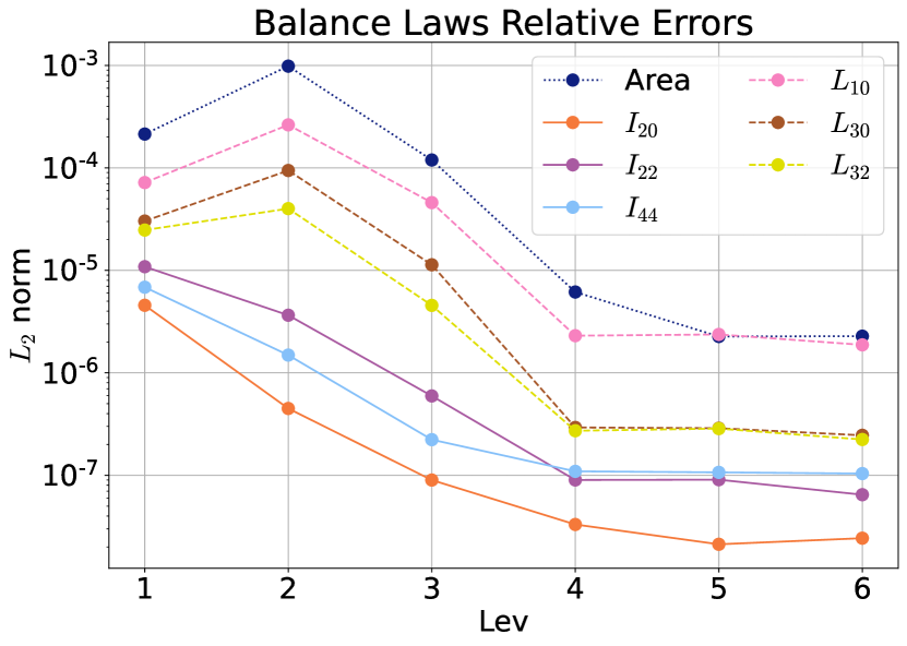
Figure 16: The convergence of relative errors in the balance laws. The horizontal axis represents the resolution labeled by “Lev”, and the vertical axis represents the $L_{2}$ norm of the relative errors in these balance laws. The blue dotted line stands for the area balance law. The solid lines are for the mass moment balance law, while the dashed lines for the spin moment balance law.

Appendix B Surface gravity

In this section, we briefly investigate the surface gravity on a dynamical horizon [30, 79, 12],

$$\kappa_{V}=-n_{b}V^{a}\nabla_{a}V^{b}.$$ (72)

Here, $n^{a}$ is the ingoing null normal to the common horizon ($t=\text{constant}$ slice) on $\mathcal{H}$, satisfying $V^{a}n_{a}=-1$. As the dynamical horizon approaches an isolated horizon, $V^{a}$ becomes null and this surface gravity coincides with the one on an isolated horizon. Because $\kappa_{V}$ is a function on a dynamical horizon, it is more convenient to consider the average value of $\kappa_{V}$ over each common horizon $\mathcal{S}$, which we denote as $\kappa_{V,t}$.

In Fig. 17, we show $\kappa_{V}$ as a function of the simulation time $t$, starting from $t=25M$. The blue solid curve represents $\kappa_{V,t}$, and the orange dashed curve represents $\max(\kappa_{V}-\kappa_{V,t})$, i.e., the maximum deviation of $\kappa_{V}$ from its average value on every $\mathcal{S}$. We see from the blue curve that $\kappa_{V,t}$ is settling down, and we check that the absolute difference between $\kappa_{V,t=400M}$ and $\kappa_{V,t=500M}$ is $\sim 10^{-5}$. The orange curve tells us that $\kappa_{V}$ is a constant on every common horizon after $t=200M$, with error $\sim 10^{-8}$. From this, we conclude that $\kappa_{V}$ already reaches a constant on the dynamical horizon at $t=500M$, with error $\sim 10^{-5}$.

The final value of $\kappa_{V}$ in our simulation is

$$\kappa_{V,t=500M}=0.221177M^{-1},$$ (73)

which is very close to the Kerr surface gravity [40, 80],

$$\kappa_{\mathrm{Kerr}}=\frac{1}{4M_{f}}-M_{f}\Omega_{H}^{2}=0.221214M^{-1}.$$ (74)

Note that this expression for $\kappa_{\mathrm{Kerr}}$ is calculated using the canonical null Killing vector of the Kerr solution on the horizon. The relative difference between $\kappa_{V,t=500M}$ and $\kappa_{\mathrm{Kerr}}$ is $1.7\times 10^{-4}$. This confirms the approximation $f\approx 1$ in Sec. III.2, and is related to the slight deviation of $\Omega_{t=500M}$ from $\Omega_{H}$ seen in Sec. IV.1.

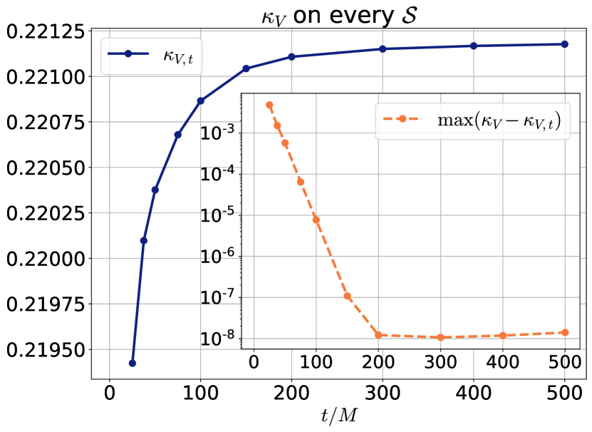
Figure 17: The temporal behavior of the surface gravity $\kappa_{V}$ on the dynamical horizon. The average value of $\kappa_{V}$, denoted by $\kappa_{V,t}$, is shown in blue/solid. The maximum deviation of $\kappa_{V}$ from $\kappa_{V,t}$ on every common horizon $\mathcal{S}$ is shown in orange/dashed in the inset. We see that $\kappa_{V}$ becomes a constant at $t=500M$.

References

- Israel [1967] W. Israel, Event horizons in static vacuum space-times, Phys. Rev. 164, 1776 (1967).
- Carter [1971] B. Carter, Axisymmetric black hole has only two degrees of freedom, Phys. Rev. Lett. 26, 331 (1971).
- Scheel et al. [2009] M. A. Scheel, M. Boyle, T. Chu, L. E. Kidder, K. D. Matthews, and H. P. Pfeiffer, High-accuracy waveforms for binary black hole inspiral, merger, and ringdown, Phys. Rev. D 79, 024003 (2009), arXiv:0810.1767 [gr-qc] .
- Campanelli et al. [2009] M. Campanelli, C. O. Lousto, and Y. Zlochower, Algebraic Classification of Numerical Spacetimes and Black-Hole-Binary Remnants, Phys. Rev. D 79, 084012 (2009), arXiv:0811.3006 [gr-qc] .
- Owen [2010] R. Owen, Degeneracy measures for the algebraic classification of numerical spacetimes, Phys. Rev. D 81, 124042 (2010), arXiv:1004.3768 [gr-qc] .
- Bhagwat et al. [2018] S. Bhagwat, M. Okounkova, S. W. Ballmer, D. A. Brown, M. Giesler, M. A. Scheel, and S. A. Teukolsky, On choosing the start time of binary black hole ringdowns, Phys. Rev. D 97, 104065 (2018), arXiv:1711.00926 [gr-qc] .
- Jaramillo et al. [2012] J. L. Jaramillo, R. Panosso Macedo, P. Moesta, and L. Rezzolla, Black-hole horizons as probes of black-hole dynamics I: post-merger recoil in head-on collisions, Phys. Rev. D 85, 084030 (2012), arXiv:1108.0060 [gr-qc] .
- Gupta et al. [2018] A. Gupta, B. Krishnan, A. Nielsen, and E. Schnetter, Dynamics of marginally trapped surfaces in a binary black hole merger: Growth and approach to equilibrium, Phys. Rev. D 97, 084028 (2018), arXiv:1801.07048 [gr-qc] .
- Prasad [2021] V. Prasad, Generalized source multipole moments of dynamical horizons in binary black hole mergers, (2021), arXiv:2109.01193 [gr-qc] .
- Ashtekar et al. [2004] A. Ashtekar, J. Engle, T. Pawlowski, and C. Van Den Broeck, Multipole moments of isolated horizons, Class. Quant. Grav. 21, 2549 (2004), arXiv:gr-qc/0401114 .
- Schnetter et al. [2006] E. Schnetter, B. Krishnan, and F. Beyer, Introduction to dynamical horizons in numerical relativity, Phys. Rev. D 74, 024028 (2006), arXiv:gr-qc/0604015 .
- Ashtekar et al. [2013] A. Ashtekar, M. Campiglia, and S. Shah, Dynamical Black Holes: Approach to the Final State, Phys. Rev. D 88, 064045 (2013), arXiv:1306.5697 [gr-qc] .
- Teukolsky [1972] S. A. Teukolsky, Rotating black holes - separable wave equations for gravitational and electromagnetic perturbations, Phys. Rev. Lett. 29, 1114 (1972).
- Teukolsky [1973] S. A. Teukolsky, Perturbations of a Rotating Black Hole. I. Fundamental Equations for Gravitational, Electromagnetic, and Neutrino-Field Perturbations, Astrophys. J. 185, 635 (1973).
- Press and Teukolsky [1973] W. H. Press and S. A. Teukolsky, Perturbations of a Rotating Black Hole. II. Dynamical Stability of the Kerr Metric, Astrophys. J. 185, 649 (1973).
- Teukolsky and Press [1974] S. A. Teukolsky and W. H. Press, Perturbations of a rotating black hole. III - Interaction of the hole with gravitational and electromagnet ic radiation, Astrophys. J. 193, 443 (1974).
- Buonanno et al. [2007] A. Buonanno, G. B. Cook, and F. Pretorius, Inspiral, merger and ring-down of equal-mass black-hole binaries, Phys. Rev. D 75, 124018 (2007), arXiv:gr-qc/0610122 .
- Berti et al. [2007] E. Berti, V. Cardoso, J. A. Gonzalez, U. Sperhake, M. Hannam, S. Husa, and B. Bruegmann, Inspiral, merger and ringdown of unequal mass black hole binaries: A Multipolar analysis, Phys. Rev. D 76, 064034 (2007), arXiv:gr-qc/0703053 .
- Giesler et al. [2019] M. Giesler, M. Isi, M. A. Scheel, and S. Teukolsky, Black Hole Ringdown: The Importance of Overtones, Phys. Rev. X 9, 041060 (2019), arXiv:1903.08284 [gr-qc] .
- Owen [2009] R. Owen, The Final Remnant of Binary Black Hole Mergers: Multipolar Analysis, Phys. Rev. D 80, 084012 (2009), arXiv:0907.0280 [gr-qc] .
- Pook-Kolb et al. [2020a] D. Pook-Kolb, O. Birnholtz, J. L. Jaramillo, B. Krishnan, and E. Schnetter, Horizons in a binary black hole merger II: Fluxes, multipole moments and stability, (2020a), arXiv:2006.03940 [gr-qc] .
- Mourier et al. [2021] P. Mourier, X. Jiménez Forteza, D. Pook-Kolb, B. Krishnan, and E. Schnetter, Quasinormal modes and their overtones at the common horizon in a binary black hole merger, Phys. Rev. D 103, 044054 (2021), arXiv:2010.15186 [gr-qc] .
- Ashtekar and Galloway [2005] A. Ashtekar and G. J. Galloway, Some uniqueness results for dynamical horizons, Adv. Theor. Math. Phys. 9, 1 (2005), arXiv:gr-qc/0503109 .
- Baumgarte et al. [1996] T. W. Baumgarte, G. B. Cook, M. A. Scheel, S. L. Shapiro, and S. A. Teukolsky, Implementing an apparent horizon finder in three-dimensions, Phys. Rev. D 54, 4849 (1996), arXiv:gr-qc/9606010 .
- Anninos et al. [1998] P. Anninos, K. Camarda, J. Libson, J. Masso, E. Seidel, and W.-M. Suen, Finding apparent horizons in dynamic 3-D numerical space-times, Phys. Rev. D 58, 024003 (1998), arXiv:gr-qc/9609059 .
- Gundlach [1998] C. Gundlach, Pseudospectral apparent horizon finders: An Efficient new algorithm, Phys. Rev. D 57, 863 (1998), arXiv:gr-qc/9707050 .
- Shoemaker et al. [2000] D. M. Shoemaker, M. F. Huq, and R. A. Matzner, Generic tracking of multiple apparent horizons with level flow, Phys. Rev. D 62, 124005 (2000), arXiv:gr-qc/0004062 .
- Thornburg [2004] J. Thornburg, A Fast apparent horizon finder for three-dimensional Cartesian grids in numerical relativity, Class. Quant. Grav. 21, 743 (2004), arXiv:gr-qc/0306056 .
- Pook-Kolb et al. [2020b] D. Pook-Kolb, O. Birnholtz, J. L. Jaramillo, B. Krishnan, and E. Schnetter, Horizons in a binary black hole merger I: Geometry and area increase, (2020b), arXiv:2006.03939 [gr-qc] .
- Ashtekar and Krishnan [2003] A. Ashtekar and B. Krishnan, Dynamical horizons and their properties, Phys. Rev. D 68, 104030 (2003), arXiv:gr-qc/0308033 .
- Ashtekar and Krishnan [2002] A. Ashtekar and B. Krishnan, Dynamical horizons: Energy, angular momentum, fluxes and balance laws, Phys. Rev. Lett. 89, 261101 (2002), arXiv:gr-qc/0207080 .
- Ashtekar and Krishnan [2004] A. Ashtekar and B. Krishnan, Isolated and dynamical horizons and their applications, Living Rev. Rel. 7, 10 (2004), arXiv:gr-qc/0407042 .
- Ashtekar et al. [2000a] A. Ashtekar, S. Fairhurst, and B. Krishnan, Isolated horizons: Hamiltonian evolution and the first law, Phys. Rev. D 62, 104025 (2000a), arXiv:gr-qc/0005083 .
- Ashtekar et al. [2000b] A. Ashtekar, C. Beetle, O. Dreyer, S. Fairhurst, B. Krishnan, J. Lewandowski, and J. Wisniewski, Isolated horizons and their applications, Phys. Rev. Lett. 85, 3564 (2000b), arXiv:gr-qc/0006006 .
- Ashtekar et al. [2002] A. Ashtekar, C. Beetle, and J. Lewandowski, Geometry of generic isolated horizons, Class. Quant. Grav. 19, 1195 (2002), arXiv:gr-qc/0111067 .
- Courant and Hilbert [1989] R. Courant and D. Hilbert, Methods of Mathematical Physics (John Wiley & Sons, Ltd, 1989).
- Baumgarte and Shapiro [2010] T. W. Baumgarte and S. L. Shapiro, Numerical Relativity: Solving Einstein’s Equations on the Computer (Cambridge University Press, 2010).
- Penrose and Rindler [1984] R. Penrose and W. Rindler, Spinors and Space-Time (Cambridge University Press, 1984).
- Owen et al. [2011] R. Owen et al., Frame-Dragging Vortexes and Tidal Tendexes Attached to Colliding Black Holes: Visualizing the Curvature of Spacetime, Phys. Rev. Lett. 106, 151101 (2011), arXiv:1012.4869 [gr-qc] .
- Wald [1984] R. M. Wald, General Relativity (Chicago Univ. Pr., Chicago, USA, 1984).
- Hawking and Hartle [1972] S. W. Hawking and J. B. Hartle, Energy and angular momentum flow into a black hole, Commun. Math. Phys. 27, 283 (1972).
- Kinnersley [1969] W. Kinnersley, Type D Vacuum Metrics, J. Math. Phys. 10, 1195 (1969).
- Leaver [1985] E. W. Leaver, An analytic representation for the quasi-normal modes of kerr black holes, Proc. R. Soc. Lond. A 402, 285–298 (1985).
- Berti et al. [2009] E. Berti, V. Cardoso, and A. O. Starinets, Quasinormal modes of black holes and black branes, Class. Quant. Grav. 26, 163001 (2009), arXiv:0905.2975 [gr-qc] .
- Isi and Farr [2021] M. Isi and W. M. Farr, Analyzing black-hole ringdowns, (2021), arXiv:2107.05609 [gr-qc] .
- Whiting [1989] B. F. Whiting, Mode stability of the kerr black hole, J. Math. Phys. 30, 1301 (1989).
- Shlapentokh-Rothman [2015] Y. Shlapentokh-Rothman, Quantitative Mode Stability for the Wave Equation on the Kerr Spacetime, Annales Henri Poincare 16, 289 (2015), arXiv:1302.6902 [gr-qc] .
- Teixeira da Costa [2020] R. Teixeira da Costa, Mode stability for the Teukolsky equation on extremal and subextremal Kerr spacetimes, Commun. Math. Phys. 378, 705 (2020), arXiv:1910.02854 [gr-qc] .
- Casals and da Costa [2021] M. Casals and R. T. da Costa, Hidden spectral symmetries and mode stability of subextremal Kerr(-dS) black holes, (2021), arXiv:2105.13329 [gr-qc] .
- Stein [2019] L. C. Stein, qnm: A Python package for calculating Kerr quasinormal modes, separation constants, and spherical-spheroidal mixing coefficients, J. Open Source Softw. 4, 1683 (2019), arXiv:1908.10377 [gr-qc] .
- Goldberg et al. [1967] J. N. Goldberg, A. J. MacFarlane, E. T. Newman, F. Rohrlich, and E. C. G. Sudarshan, Spin s spherical harmonics and edth, J. Math. Phys. 8, 2155 (1967).
- Hartle and Wilkins [1974] J. B. Hartle and D. C. Wilkins, Analytic properties of the Teukolsky equation, Commun. Math. Phys. 38, 47–63 (1974).
- Breuer et al. [1977] R. A. Breuer, J. Ryan, M. P., and S. Waller, Some Properties of Spin-Weighted Spheroidal Harmonics, Proc. R. Soc. Lond. A. 358, 71 (1977).
- Bhagwat et al. [2020] S. Bhagwat, X. J. Forteza, P. Pani, and V. Ferrari, Ringdown overtones, black hole spectroscopy, and no-hair theorem tests, Phys. Rev. D 101, 044033 (2020), arXiv:1910.08708 [gr-qc] .
- Dhani [2021] A. Dhani, Importance of mirror modes in binary black hole ringdown waveform, Phys. Rev. D 103, 104048 (2021), arXiv:2010.08602 [gr-qc] .
- [56] http://www.black-holes.org/SpEC.html.
- Lindblom et al. [2006] L. Lindblom, M. A. Scheel, L. E. Kidder, R. Owen, and O. Rinne, A New generalized harmonic evolution system, Class. Quant. Grav. 23, S447 (2006), arXiv:gr-qc/0512093 .
- Lovelace et al. [2008] G. Lovelace, R. Owen, H. P. Pfeiffer, and T. Chu, Binary-black-hole initial data with nearly-extremal spins, Phys. Rev. D 78, 084017 (2008), arXiv:0805.4192 [gr-qc] .
- Szilagyi et al. [2009] B. Szilagyi, L. Lindblom, and M. A. Scheel, Simulations of Binary Black Hole Mergers Using Spectral Methods, Phys. Rev. D 80, 124010 (2009), arXiv:0909.3557 [gr-qc] .
- Pretorius [2005] F. Pretorius, Numerical relativity using a generalized harmonic decomposition, Class. Quant. Grav. 22, 425 (2005), arXiv:gr-qc/0407110 .
- Hemberger et al. [2013] D. A. Hemberger, M. A. Scheel, L. E. Kidder, B. Szilágyi, G. Lovelace, N. W. Taylor, and S. A. Teukolsky, Dynamical Excision Boundaries in Spectral Evolutions of Binary Black Hole Spacetimes, Class. Quant. Grav. 30, 115001 (2013), arXiv:1211.6079 [gr-qc] .
- Scheel et al. [2015] M. A. Scheel, M. Giesler, D. A. Hemberger, G. Lovelace, K. Kuper, M. Boyle, B. Szilágyi, and L. E. Kidder, Improved methods for simulating nearly extremal binary black holes, Class. Quant. Grav. 32, 105009 (2015), arXiv:1412.1803 [gr-qc] .
- Rinne et al. [2007] O. Rinne, L. Lindblom, and M. A. Scheel, Testing outer boundary treatments for the Einstein equations, Class. Quant. Grav. 24, 4053 (2007), arXiv:0704.0782 [gr-qc] .
- Scheel et al. [2006] M. A. Scheel, H. P. Pfeiffer, L. Lindblom, L. E. Kidder, O. Rinne, and S. A. Teukolsky, Solving Einstein’s equations with dual coordinate frames, Phys. Rev. D 74, 104006 (2006), arXiv:gr-qc/0607056 .
- Buchman et al. [2012] L. T. Buchman, H. P. Pfeiffer, M. A. Scheel, and B. Szilagyi, Simulations of non-equal mass black hole binaries with spectral methods, Phys. Rev. D 86, 084033 (2012), arXiv:1206.3015 [gr-qc] .
- Lovelace et al. [2011] G. Lovelace, M. A. Scheel, and B. Szilagyi, Simulating merging binary black holes with nearly extremal spins, Phys. Rev. D 83, 024010 (2011), arXiv:1010.2777 [gr-qc] .
- Szilágyi [2014] B. Szilágyi, Key Elements of Robustness in Binary Black Hole Evolutions using Spectral Methods, Int. J. Mod. Phys. D 23, 1430014 (2014), arXiv:1405.3693 [gr-qc] .
- Buonanno et al. [2011] A. Buonanno, L. E. Kidder, A. H. Mroue, H. P. Pfeiffer, and A. Taracchini, Reducing orbital eccentricity of precessing black-hole binaries, Phys. Rev. D 83, 104034 (2011), arXiv:1012.1549 [gr-qc] .
- Boyle et al. [2019] M. Boyle et al., The SXS Collaboration catalog of binary black hole simulations, Class. Quant. Grav. 36, 195006 (2019), arXiv:1904.04831 [gr-qc] .
- Varma and Scheel [2018] V. Varma and M. A. Scheel, Constructing a boosted, spinning black hole in the damped harmonic gauge, Phys. Rev. D 98, 084032 (2018), arXiv:1808.07490 [gr-qc] .
- Iozzo et al. [2021a] D. A. B. Iozzo et al., Comparing Remnant Properties from Horizon Data and Asymptotic Data in Numerical Relativity, Phys. Rev. D 103, 124029 (2021a), arXiv:2104.07052 [gr-qc] .
- Boyle and Mroue [2009] M. Boyle and A. H. Mroue, Extrapolating gravitational-wave data from numerical simulations, Phys. Rev. D 80, 124045 (2009), arXiv:0905.3177 [gr-qc] .
- Boyle [2013] M. Boyle, Angular velocity of gravitational radiation from precessing binaries and the corotating frame, Phys. Rev. D 87, 104006 (2013), arXiv:1302.2919 [gr-qc] .
- Boyle et al. [2014] M. Boyle, L. E. Kidder, S. Ossokine, and H. P. Pfeiffer, Gravitational-wave modes from precessing black-hole binaries, (2014), arXiv:1409.4431 [gr-qc] .
- Boyle [2016] M. Boyle, Transformations of asymptotic gravitational-wave data, Phys. Rev. D 93, 084031 (2016), arXiv:1509.00862 [gr-qc] .
- Iozzo et al. [2021b] D. A. B. Iozzo, M. Boyle, N. Deppe, J. Moxon, M. A. Scheel, L. E. Kidder, H. P. Pfeiffer, and S. A. Teukolsky, Extending gravitational wave extraction using Weyl characteristic fields, Phys. Rev. D 103, 024039 (2021b), arXiv:2010.15200 [gr-qc] .
- Hartle [1974] J. B. Hartle, Tidal shapes and shifts on rotating black holes, Phys. Rev. D 9, 2749 (1974).
- Berti and Klein [2014] E. Berti and A. Klein, Mixing of spherical and spheroidal modes in perturbed Kerr black holes, Phys. Rev. D 90, 064012 (2014), arXiv:1408.1860 [gr-qc] .
- Booth and Fairhurst [2007] I. Booth and S. Fairhurst, Isolated, slowly evolving, and dynamical trapping horizons: Geometry and mechanics from surface deformations, Phys. Rev. D 75, 084019 (2007), arXiv:gr-qc/0610032 .
- Good and Ong [2015] M. R. R. Good and Y. C. Ong, Are black holes springlike?, Phys. Rev. D 91, 044031 (2015), arXiv:1412.5432 [gr-qc] .