The effect of tilt on turbulent thermal convection for a heated soap bubble

Abstract

We use direct numerical simulation (DNS) to explore the effect of tilt on two-dimensional turbulent thermal convection on a half-soap bubble that is heated at its equator. In the DNS, the bubble is tilted by an angle $\delta\in[0^{\circ},90^{\circ}]$, the Rayleigh number is varied between $Ra\in[3\times 10^{6},3\times 10^{9}]$, and the Prandlt number is fixed at $Pr=7$. The DNS reveals two qualitatively different flow regimes: the dynamic plume regime (DPR) and the stable plume regime (SPR). In the DPR, small dynamic plumes constantly emerge from random locations on the equator and dissipate on the bubble. In the SPR, the flow is dominated by a single large and stable plume rising from the lower edge of the bubble. The scaling behaviour of the Nusselt number $Nu$ and Reynolds number $Re$ are different in these two regimes, with $Nu\propto Ra^{0.3}$ for the DPR and $Nu\propto Ra^{0.24}$ for the SPR. Concerning $Re$, the scaling in the DPR lies between $Re\propto Ra^{0.48}$ and $Re\propto Ra^{0.53}$ depending on $Ra$ and $\delta$, while in the SPR, the scaling lies between $Re\propto Ra^{0.44}$ and $Re\propto Ra^{0.45}$ depending on $\delta$. The turbulent thermal and kinetic energy dissipation rates ($\epsilon_{T^{\prime}}$ and $\epsilon_{u^{\prime}}$, respectively) are also very different in the DPR and SPR. The probability density functions (PDF) of the normalized $\log\epsilon_{T^{\prime}}$ and $\log\epsilon_{u^{\prime}}$ are close to a Gaussian PDF for small fluctuations, but deviate considerably from a Gaussian at large fluctuations in the DPR. In the SPR, the PDFs of normalized $\log\epsilon_{T^{\prime}}$ and $\log\epsilon_{u^{\prime}}$ deviate considerably from a Gaussian PDF even for small values. The globally averaged thermal energy dissipation rate due to the mean temperature field was shown to exhibit the scaling $\langle\epsilon_{\langle T\rangle}\rangle_{\mathcal{B}}\propto Ra^{-0.23}$ in the DPR, and $\langle\epsilon_{\langle T\rangle}\rangle_{\mathcal{B}}\propto Ra^{-0.28}$ in the SPR. The globally averaged kinetic energy dissipation rate due to the mean velocity field is shown to exhibit the scaling $\langle\epsilon_{\langle u\rangle}\rangle_{\mathcal{B}}\propto Ra^{-0.47}$ in the DPR (the exponent reduces from $0.47$ to $0.43$ as $\delta$ is increased up to $30^{\circ}$). In the SPR, the behavior changes considerably to $\langle\epsilon_{\langle u\rangle}\rangle_{\mathcal{B}}\propto Ra^{-0.27}$. For the turbulent dissipation rates, the results indicate the scaling $\langle\epsilon_{T^{\prime}}\rangle_{\mathcal{B}}\propto Ra^{-0.18}$ and $\langle\epsilon_{u^{\prime}}\rangle_{\mathcal{B}}\propto Ra^{-0.29}$ in the DPR. However, the dependencies of $\langle\epsilon_{T^{\prime}}\rangle_{\mathcal{B}}$ and $\langle\epsilon_{u^{\prime}}\rangle_{\mathcal{B}}$ on $Ra$ cannot be described by power-laws in the SPR.

I Introduction

Turbulent thermal convection is ubiquitous in nature and plays a significant role in large scale flows on the Earth, such as the cyclones in the atmosphere and the circulation of the deep oceans(Lohse and Xia, 2010). Convective flows are also vital for a great number of industrial applications, for example cooling systems on chip-boardsGuo et al. (2022). The fluid motion in turbulent thermal convection is driven by buoyancy which arises due to temperature gradients imposed by boundary conditions(Ahlers, Grossmann, and Lohse, 2009). In these flows, the buoyancy force typically injects energy into the large flow structures, and this energy is then (on average) transferred to smaller scales by the energy cascade, and is finally dissipated at the smallest scales Xu, Shi, and Xi (2019). The rate of energy dissipation regulates both the global energy balances and the local fluctuations of flow quantitiesHe, Ching, and Tong (2011); Petschel et al. (2015, 2013), and studying its behavior provides insights into the fundamental properties of turbulent convective flows Zhang, Zhou, and Sun (2017); Hertlein and du Puits (2021).

I.1 Dissipation in RBC

Rayleigh-Bénard convection (RBC) is the canonical model system for fundamental studies of turbulent thermal convection (Ahlers, Grossmann, and Lohse, 2009; Stevens, Clercx, and Lohse, 2013), and the physical mechanisms and flow properties of RBC have been studied extensively in recent decades Zhang, Zhou, and Sun (2017). For a given flow configuration, the dynamics of RBC is controlled by two non-dimensional parameters, the Rayleigh number $Ra$ and the Prandlt number $Pr$. $Ra$ is defined as the non-dimensional heating temperature as:

$$Ra=\frac{{g}\beta{T}_{c}{H}^{3}}{{\nu}{\kappa}},$$ (1)

where ${T}_{c}$ is the difference between the temperature at the upper and lower boundaries, ${H}$ is the distance between the upper and lower boundaries, ${g}$ denotes the norm of the gravity acceleration, ${\beta}$ the coefficient of thermal expansion, ${\nu}$ the kinetic viscosity, and ${\kappa}$ the thermal diffusivity. $Pr$ is defined as the ratio of the momentum diffusivity to the thermal diffusivity as:

$$Pr=\frac{{\nu}}{{\kappa}}.$$ (2)

The resulting flow properties of RBC in terms of the global heat flux and nature of the fluid motion are measured by the Nusselt number $Nu$ and Reynold number $Re$, respectively. $Nu$ is the non-dimensional heat flux defined as:

$$Nu=\frac{Q}{\lambda\frac{{T}_{c}}{{H}}},$$ (3)

where $\lambda$ denotes the thermal conductivity of the fluid and $Q$ is the heat flux through the fluid. $Re$ is defined as:

$$Re=\frac{{u}_{c}{H}}{{\nu}},$$ (4)

where ${u}_{c}$ denotes a characteristic velocity of the flow, e.g. the root-mean-square velocity. A crucial open topic in RBC is to understand how the control parameters $Ra$ and $Pr$ determine the response parameters $Nu$ and $Re$, which are emergent properties of the RBC flow. Central to understanding this is to understand the behavior of the thermal and kinetic dissipation rates which are defined as

$$\epsilon_{{T}}={\kappa}\|\bm{\nabla}{T}\|^{2},$$ (5)

and

$$\epsilon_{{u}}=\frac{1}{2}{\nu}\|{\left(\bm{\nabla}{\bm{u}}+\bm{\nabla}{\bm{u}}^{\top}\right)}\|^{2},$$ (6)

where ${T}$ is the temperature field and ${\bm{u}}$ the fluid velocity.

In RBC, the following exact relations can be derivedShraiman and Siggia (1990); Siggia (1994):

$$\langle\epsilon_{{T}}\rangle_{V}={\kappa}\frac{({T}_{c})^{2}}{{H}^{2}}Nu,$$ (7)

$$\langle\epsilon_{{u}}\rangle_{V}=\frac{{\nu}^{3}}{{H}^{4}}\left(Nu-1\right)\frac{Ra}{Pr^{2}},$$ (8)

where the operator $\langle\cdot\rangle_{V}$ denotes a volume average. These exact relations connect the controlling parameters $Ra,Pr$ to the response parameters $Nu$ via $\epsilon_{{T}}$ and $\epsilon_{{u}}$. In addition, they are also foundational to the famous Grossmann-Lohse(GL) theoryGrossmann and Lohse (2000, 2001, 2002, 2004). In the original scenario proposed by the GL theory, $\langle\epsilon_{{T}}\rangle_{V}$ and $\langle\epsilon_{{u}}\rangle_{V}$ are decomposed into the contributions due to the boundaries and bulk respectivelyGrossmann and Lohse (2000, 2001, 2002). Later, Grossmann and Lohse extend the physical pictures of heat transport and include the contribution of plumesGrossmann and Lohse (2004). In macroscopic perspective, the GL theory successfully reveals the mathematical form of $Nu$ and $Re$ as functions of $Ra$ and $Pr$. However, understanding the microscopic physical mechanisms of heat transport and flow dynamics still needs the insights offered by a deep and detailed investigation of $\epsilon_{T}$ and $\epsilon_{u}$He and Tong (2009); Zhang, Zhou, and Sun (2017); Xu, Shi, and Xi (2019).

Measuring $\epsilon_{{u}}$ requires the simultaneous measurement of all 5 (for incompressible flow) components of strain-rate tensor, and $\epsilon_{{T}}$ requires the simultaneous measurements all 3 components of $\bm{\nabla}T$. Therefore, it is very challenging to measure $\epsilon_{{u}}$ and $\epsilon_{{T}}$ in experiments, and only recently has this been done. For $1\times 10^{9}\leq Ra\leq 1\times 10^{10}$, He et al.He, Tong, and Xia (2007) achieved the first successful experimental measurement of $\epsilon_{{T}}$ using a local temperature gradient probe in a cylinderical convection cell. In their results, the spatial and temporal average thermal dissipation rate $\langle\epsilon_{{T}}\rangle$ is decomposed into two components $\epsilon_{\langle T\rangle}={\kappa}\|\bm{\nabla}\langle{T}\rangle\|^{2}$ and $\langle\epsilon_{{T}^{\prime}}\rangle=\langle\epsilon_{{T}}\rangle-\epsilon_{\langle{T}\rangle}$ where $\langle\cdot\rangle$ denotes a spatially local temporal average(He, Tong, and Xia, 2007). Their results showed that $\langle\epsilon_{{T}^{\prime}}\rangle$ is dominant in the central region of the flow and therefore that the plumes makes a crucial contribution to the total dissipation in this region(He, Tong, and Xia, 2007). By contrast, the contribution from $\epsilon_{\langle{T}\rangle}$ is dominant in the thermal boundary layers (He, Tong, and Xia, 2007). The probability density function (PDF) of $\epsilon_{{T}^{\prime}}$ measured in the experimentsHe, Tong, and Xia (2007); He and Tong (2009) are well described by stretched exponential functions. In the central region of the flow or near the side walls, the PDFs of normalized $\log\epsilon_{{T}^{\prime}}$ are well described by a Gaussian PDF for relatively small values of the normalized variable(He and Tong, 2009).

Concerning $\epsilon_{{u}}$, Ni et al.Ni, Huang, and Xia (2011) measured its temporal and volume average in the center of a convection cell using particle image velocimetry (PIV). Their results validate the crucial assumption made by the GL theory, namely that the flow volume averaged dissipation is dominated by the contribution from the the boundary layersNi, Huang, and Xia (2011). Recently, Chilla et al.Méthivier et al. (2022) utilized correlation image velocimetry (CIV) technology and Fluorinert $FC770$ as the working fluid in order to measure $\epsilon_{{u}}$ with $Ra$ up to $2\times 10^{12}$. They found that power-law dependence of $\epsilon_{{u}}$ on $Re$ is $\epsilon_{{u}}\propto Re^{\frac{5}{2}}$ for laminar convection and $\epsilon_{{u}}\propto Re^{3}$ for turbulent convectionMéthivier et al. (2022).

Verzicco et al.Verzicco and Camussi (2003); Verzicco (2003) calculated $\epsilon_{{T}}$ and $\epsilon_{{u}}$ from the three dimensional temperature and velocity field obtained from DNS and also found that the dominant contribution to the globally average dissipation comes from the boundary layer, confirming the hypothesis of the GL theoryVerzicco and Camussi (2003); Verzicco (2003). Shishkina et al.Shishkina and Wagner (2006, 2007, 2008) used $\epsilon_{{T}}$ to develop a method for the extraction of plumes from the bulk flow in RBC using DNS data. For $10^{7}\leq Ra\leq 10^{9}$ and $Pr=0.7$, Emran and SchumacherEmran and Schumacher (2008) found that the PDF of normalized $\log\epsilon_{T}$ deviates from a Guassian distribution at large values of the normalized variable. It was also shown that the PDFs of $\epsilon_{{T}}$ can be fitted by stretched exponential functionsEmran and Schumacher (2008). Zhang et al.Zhang, Zhou, and Sun (2017) systematically studied the statistics of $\epsilon_{{T}}$ and $\epsilon_{{u}}$ in a two-dimensional square convection cell for $10^{6}\leq Ra\leq 10^{10}$. They obtained PDFs for $\epsilon_{{T}}$ and $\epsilon_{{u}}$ that were very similar to those of Emran and SchumacherEmran and Schumacher (2008). However, they also found deviations from the GL theory with respect to contributions to the dissipation from the central flow region of RBC(Zhang, Zhou, and Sun, 2017). Xu et al.Xu, Shi, and Xi (2019) studied the statistics of $\epsilon_{{T}}$ for RBC with very low $Pr=0.025$ and obtained similar results to those of Zhang et al.Zhang, Zhou, and Sun (2017) and EmranEmran and Schumacher (2008), suggesting that at least some of the normalized statistical properties of $\epsilon_{{T}}$ are independent of $Pr$ over the range spanned by these studies. In addition, Shashwat et al.Bhattacharya, Samtaney, and Verma (2019) studied the scaling of the thermal dissipation, both averaged only inside the boundary layer $\langle\epsilon_{{T}}\rangle_{BL}$ and only inside the bulk $\langle\epsilon_{{T}}\rangle_{BK}$, as a function of $Ra$ and for a a wide range of $Pr$. They again found that $\langle\epsilon_{{T}}\rangle_{BL}$ is much larger than $\langle\epsilon_{{T}}\rangle_{BK}$Bhattacharya, Samtaney, and Verma (2019), in line with previous studies and the GL theoryVerzicco and Camussi (2003); Verzicco (2003). They also found that a stretched exponential function accurately describes the PDFs of $\epsilon_{{T}}$ measured in both the boundary layer and the bulkBhattacharya, Samtaney, and Verma (2019).

I.2 Tilted RBC

Since geopotential lines rarely coincide with the surface of the earth(Hideo, 1984), most buoyancy-driven flows in nature are subject to a non-vertical mean temperature gradient Bejan (2013). Examples of where this is important are for mantle plumes(Taylor and McLennan, 1995; Wortel and Spakman, 2000; Condie, 2008) and atmospheric circulations(Emanuel, David Neelin, and Bretherton, 1994). It can also be of importance in engineering applications(Madanan and Goldstein, 2019). The impact of this non-vertical mean temperature gradient can be explored in a canonical setting by inclining the RBC flow by an angle $\delta$ that is varied, so that the mean temperature gradient is misaligned with gravity (with $\delta=0^{\circ}$ denoting the non-tilted case).

Ahlers et al.Ahlers, Brown, and Nikolaenko (2006) showed in experiments that the large scale circulations (LSC) are accelerated when $\delta$ is small but finite, and in a rectangular cell, the shape of the LSC is modified due to the increase of $\delta$ in DNS(Guo et al., 2015). In the numerical study of Wang et alWang et al. (2018a, b), the LSC transform from the double rolls to a single roll when $\delta$ is increased, and increasing $\delta$ can also lead to the reversal of the LSC(Wang et al., 2018b). $Re$ and $Nu$ are also influenced by $\delta$. In DNS, Guo et al.Guo et al. (2015) found that as $\delta$ is increased from $0^{\circ}$ to $90^{\circ}$, $Re$ first increases then drops after reaching a maximum, while $Nu$ decreases monotonically, with a maximum decrease of $18\%$. By means of experiments, Wei et al.Wei and Xia (2013) measured $Re$ as a function of $Ra$ for $0.5^{\circ}\leq\delta\leq 3.4^{\circ}$ and found the scaling $Re\sim Ra^{0.43}$ (or $Re\sim Ra^{0.55}$ depending on the definition of $Re$) independent of $\delta$ for these small inclination angles. The experimental study of Ahlers et al.(Ahlers, Brown, and Nikolaenko, 2006) showed that for small $\delta$, $Nu\sim Re^{\frac{1}{3}}$, with only slight variations with $\delta$. By means of DNS, Shishkina et al.Shishkina and Horn (2016) and Zwirner et al.Zwirner and Shishkina (2018) considered a wide range of $Ra$, $Pr$ and $\delta$. The results demonstrated that $Nu$ depends on $\delta$ in a complicated, non-monotonic way when $\delta$ is varied over a large rangeShishkina and Horn (2016); Zwirner and Shishkina (2018). Recently, with help of both DNS and experiments, Zhang et al.Zhang, Ding, and Xia (2021) studied tilted RBC systematically and to elucidate how the misalignment of the mean temperature gradient with gravity influences the flow. In their study, $Ra$ is decomposed into a vertical Rayleigh number $Ra_{V}$ and a horizontal Rayleigh number $Ra_{H}$, and $Nu$ is also decomposed into a vertical Nusselt number $Nu_{V}$ and a horizontal Nusselt number $Nu_{H}$. By taking the effect of the misalignment into consideration, Zhang et al.Zhang, Ding, and Xia (2021) extended the classical GL theory and predicted $Nu_{V}$ as a function of $Re$, $Pr$ and $\delta$.

I.3 Soap bubble

While the classical RBC setup has been the subject of intense investigation, in many naturally occurring contexts the thermal convection takes place in curved or spherical geometries. Understanding the influence of this curved geometry on the thermal convection is therefore of great importance for geophysics and astrophysics(Kellay, 2017). A canonical setup for exploring this is to consider turbulent thermal convection on a half soap bubble that is heated at its equator, and this was first studied experimentally by KellayKellay (2017). Since the thickness of the soap film is negligible compared to the radius of the bubble, the turbulent flow on the bubble corresponds to quasi two-dimensional turbulence on a hemispherical surfaceKellay and Goldburg (2002); Kellay (2017). The experiments revealed that on the bubble there form large, persistent and isolated vorticesSeychelles et al. (2008, 2010); Meuel et al. (2018) which are similar to typhoons or cyclones that occur in the atmosphereMeuel et al. (2012, 2013). Indeed, several studies revealed important quantitative similarities of the trajectories and intensities of these vorticites on the bubble with those of cyclones in nature Seychelles et al. (2008, 2010); Meuel et al. (2012, 2013, 2018). In fact, the trajectories of the cyclones are successfully predicted by a method first developed to describe that of the vortex on the bubbleMeuel et al. (2012). DNS of the half soap bubble were first performed by Xiong et al.Xiong, Fischer, and Bruneau (2012), and Bruneau et al.Bruneau et al. (2018) used the DNS to show that the scaling behaviour of $Re$ and $Nu$ are very similar to that in standard RBC, with the DNS yielding $Nu\sim Ra^{0.30}$ and $Nu\sim Ra^{0.49}$. He et al.He et al. (2021) further extended the model to investigate the impact of bubble rotation on the convective flow and showed that $Nu$ is not effected by even strong rotation, while $Re$ decreases considerably with increasing rotation (He et al., 2021).

An important open issue is how the convective flow on the soap bubble is affected by inclining the bubble, analogous to the tilted RBC discussed earlier. The impact of the tilting could be different from that for standard RBC because the curved surface on the bubble leads to a spatial dependence of the alignment of gravity with the flow direction.

I.4 Organization of the paper

The aim of our study is to fill this gap by investigating the effect of tilt on the thermal convection of the soap bubble flow. Special focus on the thermal and kinetic dissipation fields due to the key role these play in governing the properties of the convective flow. In section 2 we introduce the governing equations and the energy budgets. In section 3, the results of the DNS are presented and discussed. Conclusions are then drawn in section 4.

II Method

II.1 Governing Equations

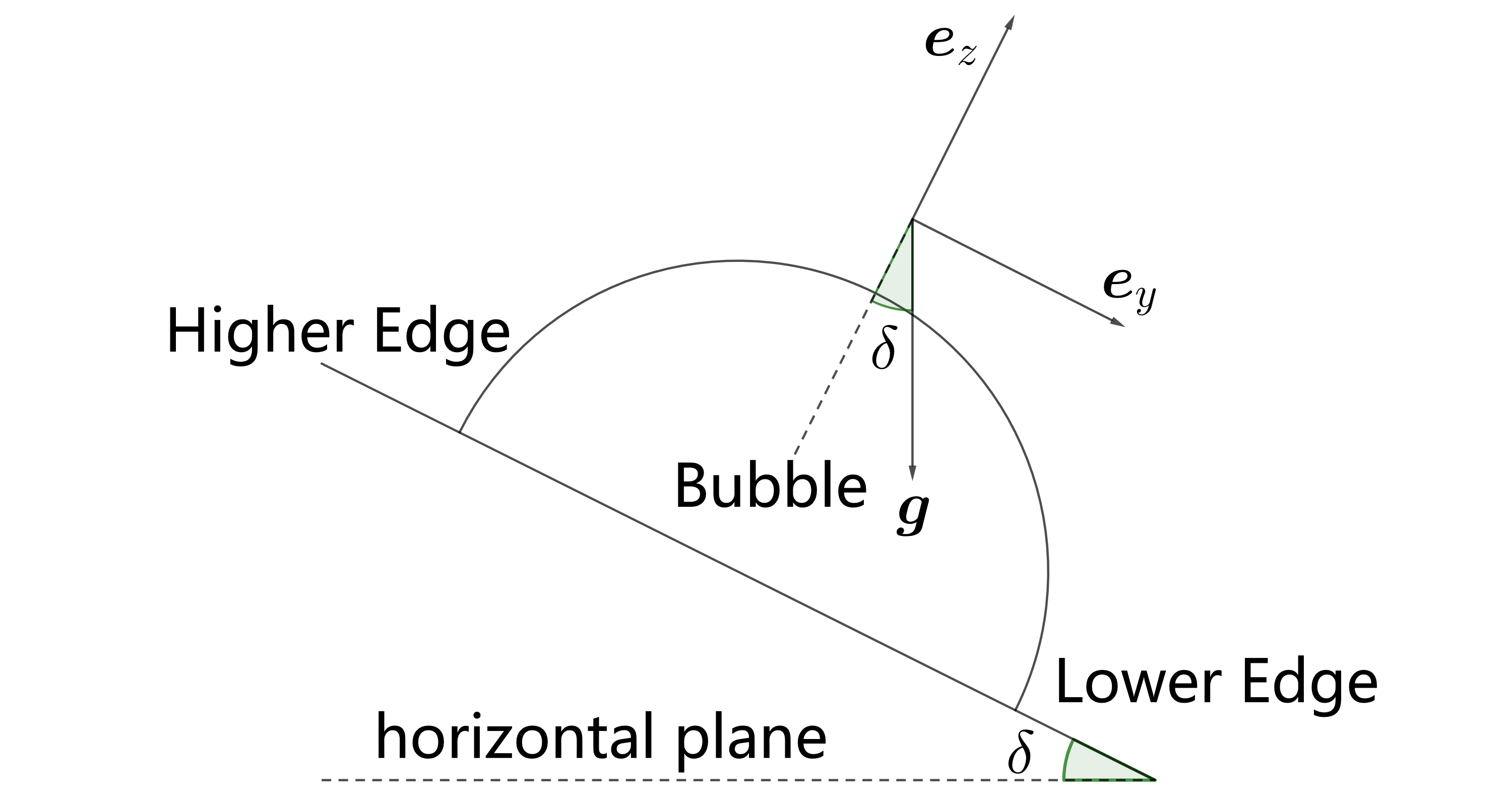
Figure 1: Illustration of the half-soap bubble and the Cartesian coordinate system used.

In our study, a half-soap bubble of radius ${R}$ is mounted on a base plane which keeps the equator of the bubble at constant temperature ${T}_{0}$, as shown in figure 1. A three dimensional Cartesian coordinate system is used whose origin is located at the center of the bubble, and is defined by the unit vector $\bm{e}_{y}$ that is parallel to the base plane, $\bm{e}_{z}$ that is orthogonal to the base plane, and $\bm{e}_{x}$ is defined such that $\bm{e}_{z}=\bm{e}_{x}\times\bm{e}_{y}$. In this system, an arbitrary vector ${\bm{a}}$ is represented in terms of its Cartesian components as $\bm{a}=a_{x}\bm{e}_{x}+a_{y}\bm{e}_{y}+a_{z}\bm{e}_{z}$. The base plane is tilted by an angle $\delta\in[0,\pi/2]$, and since the gravitational acceleration vector $\bm{g}$ is fixed we have $\bm{e}_{g}\equiv\bm{g}/\|\bm{g}\|=(\bm{e}_{y}\sin\delta-\bm{e}_{z}\cos\delta)$.

The thickness of the soap film is negligible compared to the radius of the bubble, and hence the bubble may be approximated as a two-dimensional hemispherical surface. The bubble is heated at the equator and cools through contact with the surrounding colder air. The variation of the mass density ${\rho}$ due to the temperature ${T}$ is assumed under the Boussinesq approximation to be ${\rho}={\rho}_{0}\left[1-{\beta}({T}-{T}_{0})\right]$, where ${\beta}$ is the thermal expansion coefficient, ${T}_{0}$ is the reference temperature on the equator, ${\rho}_{0}$ is the massive density of the fluid when $T=T_{0}$. For this model, the governing equations for the flow are given by the Boussinesq-Navier-Stokes system:

$$\bm{\nabla}\cdot{\bm{u}}=0,$$ (9)

$$\partial_{t}{\bm{u}}+({\bm{u}}\cdot\nabla){\bm{u}}=-\frac{1}{{\rho}_{0}}\bm{\nabla}{p}+{\nu}\nabla\cdot\left(\bm{\nabla}{\bm{u}}+\bm{\nabla}{\bm{u}}^{\top}\right)-{\beta}({T}-{T}_{0}){\bm{g}}-{F}{\bm{u}},$$ (10)

$$\partial_{t}{T}+({\bm{u}}\cdot\nabla){T}={\kappa}\nabla^{2}{T}-{S}{T},$$ (11)

where ${\bm{u}}$ is the fluid velocity and ${p}$ is the pressure field that includes the hydrostatic contribution.

The terms involving ${S}$ and ${F}$ are the external cooling and friction terms, respectively, which model the heat exchange and friction due to the the cold air surrounding the bubble. These terms are required in order for the DNS to attain non-trivial steady-state regimes, and are discussed in details in the study of Bruneau et al.Bruneau et al. (2018) and He et al.He et al. (2021). Analogous terms are also routinely used when performing DNS of two-dimension turbulence on flat geometries Boffetta and Ecke (2012).

The equations can be non-dimensonlized using the radius of the bubble ${R}$, the initial temperature difference between the equator and the North pole $\Delta{T}$, and the free fall velocity ${u}_{c}=\sqrt{g\beta\Delta{T}{R}}$ leading to (for notational simplicity, the non-dimensional independent variables are not indicated by a “hat” symbol, and all variables are to be understood as non-dimensional hereafter)

$$\bm{\nabla}\cdot\bm{u}=0,$$ (12)

$$\partial_{t}\bm{u}+(\bm{u}\cdot\nabla)\bm{u}=-\bm{\nabla}p+\frac{1}{\sqrt{Ra/Pr}}\nabla^{2}\bm{u}-\frac{(T-T_{0})}{T_{0}}\bm{e}_{g}-F\bm{u},$$ (13)

$$\partial_{t}T+(\bm{u}\cdot\nabla)T=\frac{1}{\sqrt{RaPr}}\nabla^{2}T-ST,$$ (14)

where the Rayleigh number and Prandlt number are defined as,

$$Ra=\frac{{g}{\beta}\Delta{T}{R}^{3}}{{\nu}{\kappa}},$$ (15)

$$Pr=\frac{{\kappa}}{{\nu}}.$$ (16)

In our DNS we use $S=0.06$ and $F=0.06$, which are the values that have already been shown to be suitable in previous studiesBruneau et al. (2018); He et al. (2021). The boundary conditions used are $\bm{u}=0$ and $T_{0}=1$ on the bubble equator.

II.2 Tilt leads to stable stratification for the hemispherical flow

The tilt of the bubble by an angle $\delta$ affects the flow dynamics only through its influence on the buoyancy term. To consider this influence, it is convenient to introduce a spherical coordinate system with coordinates $(r,\theta,\phi)$, and basis vectors $\bm{e}_{r}(\theta,\phi)$, $\bm{e}_{\theta}(\theta,\phi)$, $\bm{e}_{\phi}(\theta,\phi)$. For the hemisphere, the polar coordinate is restricted to $\theta\in[0,\pi/2]$ and is measured from the $\bm{e}_{z}$ axis, while the azimuthal coordinate $\phi\in[0,2\pi)$ is measured from the $\bm{e}_{x}$ axis. For our two-dimensional flow on the bubble surface, the motion is confined to $r=R$, and there is no flow in the radial direction $\bm{e}_{r}(\theta,\phi)$. The unit vector $\bm{e}_{\theta}(\theta,\phi)$ depends on the coordinates as

$$\bm{e}_{\theta}(\theta,\phi)=\bm{e}_{x}\cos\theta\cos\phi+\bm{e}_{y}\cos\theta\sin\phi-\bm{e}_{z}\sin\theta,$$ (17)

and therefore when the flow equations are projected onto the direction $\bm{e}_{\theta}(\theta,\phi)$, the buoyancy force projected along this direction (denoted by $B_{\theta}$) becomes

$$\begin{split}B_{\theta}=-\frac{(T-T_{0})}{T_{0}}\Big{(}\sin\delta\cos\theta\sin\phi+\cos\delta\sin\theta\Big{)}.\end{split}$$ (18)

For the no tilt case $\delta=0$ we have $B_{\theta}=-((T-T_{0})/T_{0})\sin\theta$. Since $\sin\theta\geq 0$ on the interval $\theta\in[0,\pi/2]$, then $B_{\theta}$ will act to accelerate the fluid in the $-\bm{e}_{\theta}$ direction in regions where the temperature anomaly is positive, $(T-T_{0})/T_{0}>0$. This means that fluid particles that are heated near the equator will accelerate towards the North pole, corresponding to convection. For $\delta=\pi/2$ then $B_{\theta}=-((T-T_{0})/T_{0})\cos\theta\sin\phi$. In this case, while $\cos\theta\geq 0$ on the interval $\theta\in[0,\pi/2]$, $\sin\phi$ changes sign on the interval $\phi\in[0,2\pi)$. Due to this, on the lower side of the hemisphere corresponding to $y>0$ and $\phi\in[0,\pi)$, $B_{\theta}$ will act to accelerate the fluid in the $-\bm{e}_{\theta}$ direction when $(T-T_{0})/T_{0}>0$, but for $\phi\in(\pi,2\pi)$, $B_{\theta}$ will act to accelerate the fluid in the $+\bm{e}_{\theta}$ direction when $(T-T_{0})/T_{0}>0$. It means that when $(T-T_{0})/T_{0}>0$, then for $\phi\in[0,\pi)$, $B_{\theta}$ will lead to convective motion towards the North pole, while for $\phi\in(\pi,2\pi)$, $B_{\theta}$ will act to stabilize and stratify the flow. Therefore, while for $\delta=0$, heating at the equator generates buoyancy forces leading to convection and (for sufficiently large $Ra$) turbulence over the entire surface of the bubbleHe et al. (2021), for $\delta=\pi/2$, buoyancy forces leading to convection and turbulence can arise for $\phi\in[0,\pi)$, whereas for $\phi\in(\pi,2\pi)$ the buoyancy forces will quench the turbulence and stratify the flow. Note also that since $B_{\theta}=-((T-T_{0})/T_{0})\cos\theta\sin\phi$, then the buoyancy forces that produce convection in the region $\phi\in[0,\pi)$ will be strongest near $\phi=\pi/2$. Hence, for $\delta=\pi/2$, we would expect to see the strongest convection and turbulence near the lower edge of the bubble.

For intermediate $\delta$, the tilt will lead to stratification at points where the inequality $\sin\delta\sin\theta\sin\phi+\cos\delta\cos\theta<0$ is satisfied, and this can only be satisfied for $\phi\in(\pi,2\pi)$ and in the region $\theta\in[0,-\tan^{-1}(\tan\delta\sin\phi))$.

III Direct Numerical Simulations

The numerical simulations are conducted by the homebrew code which is introduced in details in previous studiesBruneau et al. (2018); He et al. (2021). Here we give a brief overview of the numerical methods used in the DNS. The nondimensional governing equations are solved numerically in a computational space which is accomplished by the stereographic projection. In the computational space, the geometry of the bubble is a plane circle where the stagger grid is employed for discretization and the penalty method is employed for the implementation of the boundary conditions. The temporal derivatives are approached by the second-order Gear scheme and the non-linear terms are handled by a third-order Murman-like scheme. The mesh sensitivity are checked and the resolution of $1024\times 1024$ and $2048\times 2048$ is choosed for the different $Ra$.

The table 1 lists the parameters for all the cases of DNS considered in this study. $F$ and $S$ are fixed to $0.06$ as in previous studiesBruneau et al. (2018); He et al. (2021); Meuel et al. (2018). $Pr$ is fixed to $7$ since the soap concentration in the water is very low. The Rayleigh number is varied in the range of $Ra\in[3\times 10^{6},3\times 10^{9}]$, and the full range of tilting angles (in degrees) $\delta\in[0^{\circ},90^{\circ}]$ is explored.

Table 1: The configuration of non-dimensional coefficients for all the cases considered in this study

$Ra$	$Pr$	$\delta$
$3\times 10^{9}$	$7$	$0^{\circ}$	$30^{\circ}$	$60^{\circ}$	$90^{\circ}$
$3\times 10^{8}$	$7$	$0^{\circ}$	$30^{\circ}$	$60^{\circ}$	$90^{\circ}$
$3\times 10^{7}$	$7$	$0^{\circ}$	$30^{\circ}$	$60^{\circ}$	$90^{\circ}$
$3\times 10^{6}$	$7$	$0^{\circ}$	$30^{\circ}$	$60^{\circ}$	$90^{\circ}$

IV Results & Discussion

IV.1 the Phenomenological Observations

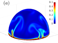
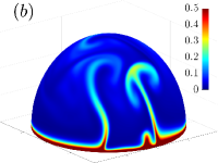
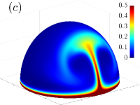
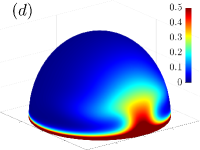
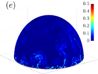
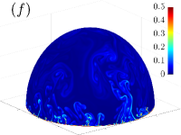
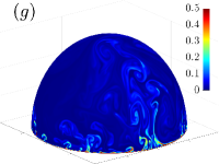
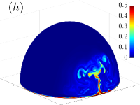
Figure 2: Snapshots of the temperature fields for $Ra=3\times 10^{6}$(the upper line: $(a)$ to $(d)$) and $Ra=3\times 10^{9}$(the lower line: $(e)$ to $(h)$) with $\delta=0^{\circ},30^{\circ},60^{\circ},90^{\circ}$(from left to right).

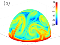
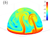
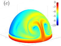
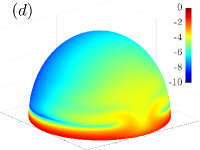
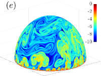
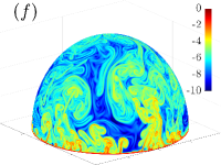
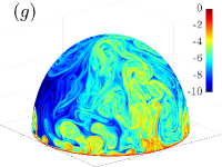
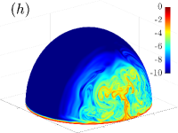
Figure 3: Snapshots of the logarithm of the thermal energy dissipation rate $\log_{10}\left(\epsilon_{T}\right)$ for $Ra=3\times 10^{6}$(the upper line: $(a)$ to $(d)$) and $Ra=3\times 10^{9}$(the lower line: $(e)$ to $(h)$) with $\delta=0^{\circ},30^{\circ},60^{\circ},90^{\circ}$(from left to right).

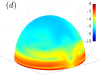
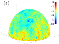
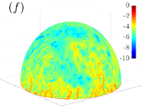
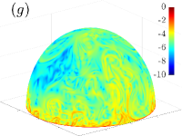
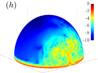
Figure 4: Snapshots of the logarithm of the kinetic energy dissipation rate $\log_{10}\left(\epsilon_{u}\right)$ for $Ra=3\times 10^{6}$(the upper line: $(a)$ to $(d)$) and $Ra=3\times 10^{9}$(the lower line: $(e)$ to $(h)$) with $\delta=0^{\circ},30^{\circ},60^{\circ},90^{\circ}$(from left to right).

We begin by making qualitative observations on the effect of $\delta$ on the behavior of instantaneous flow fields on the bubble. Figure 2 illustrates typical snapshots of the temperature field $T$ on the surface of the bubble for different Rayleigh numbers $Ra$ and tilt angles $\delta$. The upper line in figure 2 is for $Ra=3\times 10^{6}$, and the lower line in figure 2 is for $Ra=3\times 10^{9}$. From left to the right, $\delta$ increases from $0^{\circ}$ to $90^{\circ}$. For the same time instant, figures 3 and 4 illustrate the corresponding fields of the logarithmic thermal energy dissipation $\log_{10}\left(\epsilon_{T}\right)$ and the logarithmic kinetic energy dissipation $\log_{10}\left(\epsilon_{u}\right)$, respectively.

Figure 2 shows that for $\delta=0^{\circ}$, the flow only features plumes and does not contain large scale circulations which are usually seen in Rayleigh-Bénard convection. This is because for the bubble, there is no cold boundary as there is in in Rayleigh-Bénard convection, but only a hot boundary at the equator. As $Ra$ is increased, the plumes become more filamented and smaller. These flow patterns appearing here for $\delta=0^{\circ}$ are qualitatively similar to those observed in experimentsSeychelles et al. (2008, 2010); Meuel et al. (2012, 2013, 2018) and DNSXiong, Fischer, and Bruneau (2012); Bruneau et al. (2018); Meuel et al. (2018); He et al. (2021).

On the other hand, the observed flow patterns go through a dramatic change as $\delta$ is increased from $0^{\circ}$ to $90^{\circ}$. When $\delta$ is relatively small, e.g. $30^{\circ}$, then the flow patterns are very similar to those for $\delta=0^{\circ}$, with dynamic plumes detaching from the boundary layer at random locations on the equator, and the plumes dissipate as time proceeds. We refer to this regime as the dynamic plumes regime (DPR). When $\delta$ is sufficiently large, however, the flow is dominated by a stable large plume that rises from the lower edge of the bubble and is persistent in time. We refer to this as the stable plume regime(SPR). It should be noted, however, that the stable plume appears as soon as $\delta>0$, however it is relatively weak and blends in with the dynamic plumes that dominate in the DPR.

The transition of the flow patterns from the DPR to the SPR as $\delta$ is increased can be understood in terms of the analysis in §II.2, where we showed that as $\delta$ is increased, convection will be suppressed in the upper half of the bubble where $\phi\in[\pi,2\pi)$, and that for the lower half where $\phi\in[0,\pi)$, the convection will be strongest near the lower edge at $\phi=\pi/2$.

The snapshots of the temperature fields also reveal that the threshold angle for the flow to transition from the DPR to the SPR depends on $Ra$. For $Ra=3\times 10^{6}$, the flow is in the SPR for $\delta\gtrsim 60^{\circ}$, while for $Ra=3\times 10^{9}$, the flow is still in the DPR for $\delta=60^{\circ}$ but has transitioned to the SPR at $\delta=90^{\circ}$. Figure 5 illustrates how the flow state depends on $\delta$ and $Ra$. The figure shows that for $\delta\leq 30^{\circ}$, the flow remains in the DPR for each $Ra$. For $\delta=60^{\circ}$, the cases with $Ra=3\times 10^{6}$ and $Ra=3\times 10^{7}$ have transitioned into the SPR while the cases with higher $Ra$ remain in the DPR. For $\delta=90^{\circ}$, however, all of the cases are in the SPR.

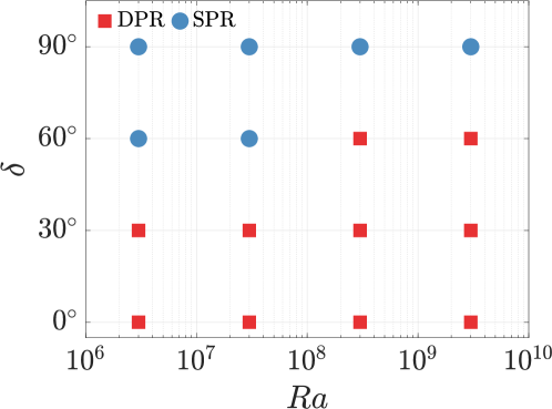
Figure 5: Schematic to illustrate how the flow state depends on $Ra$ and $\delta$.

Comparing figures 3 and 4 with figure 2 shows that the plumes are closely associated with regions of large thermal and kinetic energy dissipation field, similar to what is observed in Rayleigh-Bénard convectionZhang, Zhou, and Sun (2017); Emran and Schumacher (2008); Xu, Shi, and Xi (2019); Shishkina and Wagner (2007). This indicates that the plumes play a key role in the dissipation of thermal and kinetic energy on the bubble, and also suggests that the dissipation rates for these two fields will be coupled. To explore this, we define the correlation coefficient between $\epsilon_{T}$ and $\epsilon_{u}$ as

$$\langle c(\bm{x})\rangle=\frac{\langle(\epsilon_{T}-\langle\epsilon_{T}\rangle)(\epsilon_{u}-\langle\epsilon_{u}\rangle)\rangle}{\sqrt{\langle(\epsilon_{T}-\langle\epsilon_{T}\rangle)^{2}\rangle}\sqrt{\langle(\epsilon_{u}-\langle\epsilon_{u}\rangle)^{2}\rangle}},$$ (19)

where $\langle\cdot\rangle$ here donates a time average at a given location $\bm{x}$ on the bubble surface.

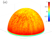
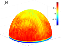
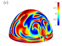
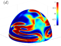
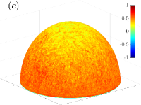
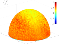
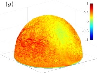
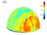
Figure 6: The distribution of $\langle c\rangle$ on the bubble for $Ra=3\times 10^{6}$(the upper line: $(a)$ to $(d)$) and $Ra=3\times 10^{9}$(the lower line: $(e)$ to $(h)$) with $\delta=0^{\circ},30^{\circ},60^{\circ},90^{\circ}$(from left to right).

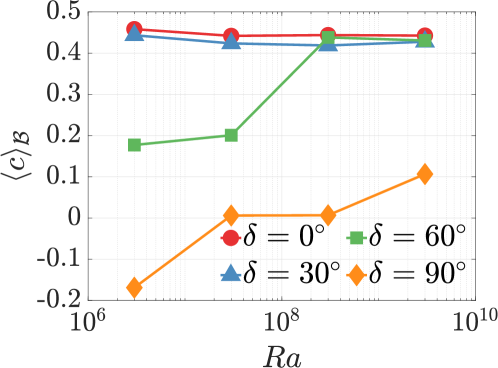
Figure 7: The global correlation coefficients corresponding to different $Ra$ and $\delta$

Figure 6 illustrates how $\langle c\rangle$ varies across the surface of the bubble as $\delta$ is varied and the flow transitions between the DPR and SPR. For the DPR, $\langle c\rangle$ is positive over most of the bubble, and over a considerable part of the surface the correlation is quite high. For the SPR, significant regions of the bubble have $\langle c\rangle<0$ when $Ra=3\times 10^{6}$, indicating significant regions of negative correlation between $\epsilon_{T}$ and $\epsilon_{u}$. However, for $Ra=3\times 10^{9}$, when $\delta=90^{\circ}$ and the flow is in the SPR, there is still, however, a significant positive correlation near the lower edge of the bubble where vigorous turbulence still exists. This differing behavior is probably due to the fact that while the SPR for $Ra=3\times 10^{9}$ is still vigorously turbulent near the lower edge of the bubble, for $Ra=3\times 10^{6}$ the flow is almost laminar.

It is seen that the SPR are characterized by the filamented and convoluted patches of high $\langle c\rangle$. The patches are more filamented and convoluted for higher $Ra$. For the DPR($(a)$, $(b)$, $(e)$, $(f)$ and $(g)$ in figure 6), $\langle c\rangle$ decreases in the domain where the stable plume occupies with $\delta$ increasing. For the SPR($(c)$, $(d)$ and $(h)$ in figure 6), the distribution of $\langle c\rangle$ is more complex. For relative small $Ra$($(c)$, $(d)$ in figure 6), the dynamic plume disappears on the bubble and there is only the stable plume on the bubble. Thus the patches of high or low $\langle c\rangle$ have large size and cover the whole surface of the bubble. But when $Ra$ is enough high($(h)$ in figure 6), the stable and dynamic plumes coexist on the bubble. $\langle c\rangle$ on the higher edge of the bubble is close to $0$. In the region near the stable plume, the patch of high $\langle c\rangle$ become filamented and convoluted as in the DPR.

Figure 7 shows the globally averaged correlation coefficient $\langle c\rangle_{\mathcal{B}}$ corresponding to all the cases in table 1. Here, the global averaging operator is defined for an arbitrary field variable ${a}(\bm{x},t)$ as

$$\langle{a}\rangle_{\mathcal{B}}=\frac{\oint_{\mathcal{B}}{a}(\bm{x},t)\mathrm{d}s}{2\pi R},$$ (20)

where $\mathrm{d}s$ is the elemental area on the bubble surface $\mathcal{B}$.

For the DPR, $\langle c\rangle_{\mathcal{B}}$ is almost independent of $Ra$ and approximately equal to $0.42$. This value validates the observation based on the instantaneous flow field that the thermal and kinetic energy dissipation rates should be correlated to each other since they are both driven by plumes in the flow. It is also interesting to note that a similar value of $\langle c\rangle_{\mathcal{B}}\approx 0.4$ was obtained for Rayleigh-Bénard convectionZhang, Zhou, and Sun (2017). Once the flow transitions from the DPR to SPR, the magnitude of $\langle c\rangle_{\mathcal{B}}$ reduces significantly, with $|\langle c\rangle_{\mathcal{B}}|\lesssim 0.2$ in the SPR.

IV.2 Nusselt $Nu$ and Reynold number $Re$

We now turn to consider the scaling relation of the Nusselt number $Nu$ and Reynolds number $Re$ versus $Ra$ in the DPR and SPR. For the bubble flow, $Nu$ is defined differently from that in RBC. In RBC, thermal energy passes through the layer of fluid and $Nu$ is defined as the non-dimensional heat flux through the fluid layer in order to quantify the efficiency of the heat transport. By contrast, in the bubble flow, heat is absorbed by the fluid at the equator and the thermal energy is dissipated entirely within the flow, with no cold boundary through which it can pass. For the bubble flow, we are therefore interested in the efficiency of the heat transport away from the equator and so $Nu$ is defined as the non-dimensional heat flux across the equatorHe et al. (2021)

$$Nu=\frac{Q_{turb}}{Q_{0}},$$ (21)

where $Q_{turb}$ is the heat flux at the equator for the turbulent flow and $Q_{0}$ is the ideal heat flux associated with pure conduction at the equator. The quantity $Q_{turb}$ is obtained by the temperature field as

$$Q_{turb}=-\langle\nabla_{z}T|_{\theta=\pi/2}\rangle.$$ (22)

The ideal heat flux of pure conduction $Q_{0}$ is the heat flux in the hypothesis that the fluid is motionless all over the bubble:

$$Q_{0}=\nabla_{z}T_{0}|_{\theta=\pi/2},$$ (23)

where $T_{0}$ is obtained as the solution to (14) using $\bm{u}=\bm{0},S=0$ and boundary conditions $T|_{\theta=\pi/2}=1$ and $T|_{\theta=0}=0$.

For evaluating $Re$, the root mean square (r.m.s) velocity $u_{rms}=\sqrt{\langle\|\bm{u}\|^{2}\rangle_{\mathcal{B}}}$ is usually used as a global measure of the turbulent velocity scale in studies of RBCZhang, Zhou, and Sun (2017); Sun and Xia (2005), and using this gives

$$Re=\sqrt{\frac{Ra}{Pr}}u_{rms}.$$ (24)

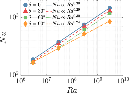
Figure 8: The variation of $Nu$ with $Ra$ and $\delta$

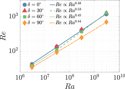
Figure 9: The variation of $Re$ with $Ra$ and $\delta$

Figures 8 and 9 show $Nu$ and $Re$ as a function of $Ra$ for different $\delta$, with power-law fits of the data illustrated by solid or dash lines. For $\delta=0^{\circ}$, the scaling relations of $Nu$ and $Re$ are $Nu\propto Ra^{0.30}$ and $Re\propto Ra^{0.48}$ respectively, which match those reported by previous studies of RBCSun and Xia (2005); Xu, Shi, and Xi (2019). As $\delta$ is increased, we observe that the scaling behaviours are strongly influenced by the flow regime. When the flow is in the DPR, $Nu$ scales with $Ra$ as a power-law form with scaling exponent close to $0.30$. As the flow transitions to the SPR, the scaling exponent for $Nu$ decreases from $0.30$ to $0.24$. Moreover, there is a strong reduction in the actual values of $Nu$ when the flow transitions from the DPR to the SPR, especially for higher $Ra$.

Concerning $Re$, for $\delta=30^{\circ}$ the dependence of $Re$ on $Ra$ is almost identical to that for the case with $\delta=0^{\circ}$ For $\delta=60^{\circ}$, the scaling relation turns into $Re\propto Ra^{0.45}$ for the DPR and $Re\propto Ra^{0.53}$ for the SPR. The data for $\delta=90^{\circ}$ can be described by a single power law $Re\propto Ra^{0.44}$ since all cases are in the SPR. There is also a considerable drop in the magnitude of $Re$ when the flow transitions from the DPR to the SPR. These results show that there is a clear quantitative effect of $\delta$ on both $Nu$ and $Re$ and their dependence on $Ra$, which corresponds to the transition the flow undergoes when moving from the DPR to the SPR as $\delta$ is increased.

IV.3 Probability density functions (PDFs) of $\epsilon_{T^{\prime}}$ and $\epsilon_{u^{\prime}}$

We now turn to consider the statistical characteristics of the turbulent thermal energy dissipation rate $\epsilon_{T^{\prime}}$ and kinetic energy dissipation rate $\epsilon_{u^{\prime}}$, which are defined as

$$\epsilon_{T^{\prime}} =\epsilon_{T}-\epsilon_{\langle T\rangle},$$ (25)

$$\epsilon_{T} ={\kappa}\|\bm{\nabla}{T}\|^{2},$$ (26)

$$\epsilon_{\langle T\rangle} ={\kappa}\|\bm{\nabla}{\langle T\rangle}\|^{2},$$ (27)

and

$$\epsilon_{u^{\prime}} =\epsilon_{u}-\epsilon_{\langle u\rangle},$$ (28)

$$\epsilon_{u} =\frac{1}{2}{\nu}\|\bm{\nabla}{\bm{u}}+\bm{\nabla}{\bm{u}}^{\top}\|^{2},$$ (29)

$$\epsilon_{\langle u\rangle} =\frac{1}{2}{\nu}\|\langle\bm{\nabla}{\bm{u}}+\bm{\nabla}{\bm{u}}^{\top}\rangle\|^{2},$$ (30)

Figure 10 show the PDFs of $\epsilon_{T^{\prime}}$ and $\epsilon_{u^{\prime}}$ for different $Ra$ with $\delta=0^{\circ}$. As is common in RBC studiesEmran and Schumacher (2008); Zhang, Zhou, and Sun (2017); Xu, Shi, and Xi (2019), $\epsilon_{T^{\prime}}$ and $\epsilon_{u^{\prime}}$ are normalized by their global root-mean-square (r.m.s) which are $\sqrt{\langle\epsilon_{T^{\prime}}\rangle}_{\mathcal{B}}$ and $\sqrt{\langle\epsilon_{u^{\prime}}\rangle}_{\mathcal{B}}$, respectively. We also plot $\log(\epsilon_{T^{\prime}})$ and $\log(\epsilon_{u^{\prime}})$ with their local mean values $\mu_{\log\epsilon_{T^{\prime}}}=\langle\log\epsilon_{T^{\prime}}\rangle$, $\mu_{\log\epsilon_{u^{\prime}}}=\langle\log\epsilon_{u^{\prime}}\rangle$ subtracted, and normalized by their local standard deviations $\sigma_{\epsilon_{T^{\prime}}}=\sqrt{\langle(\log\epsilon_{T^{\prime}}-\mu_{\log\epsilon_{T^{\prime}}})^{2}\rangle}$, $\sigma_{\epsilon_{u^{\prime}}}=\sqrt{\langle(\log\epsilon_{u^{\prime}}-\mu_{\log\epsilon_{u^{\prime}}})^{2}\rangle}$, in order to consider how close the random variables are to being log-Normally distributed. In the figures for the logarithmic variables, the solid lines show a standardized Gaussian PDF for the reference.

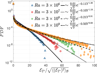
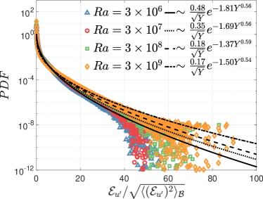
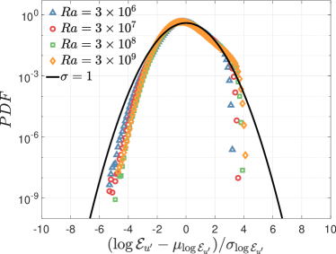
Figure 10: the PDFs of $\epsilon_{T^{\prime}}$ and $\epsilon_{u^{\prime}}$ with different $Ra$ for $\delta=0^{\circ}$

The results show that the PDFs of $\epsilon_{T^{\prime}}$ and $\epsilon_{u^{\prime}}$ have increasingly wider tails as $Ra$ is increased. This indicates increasing small-scale intermittency in the fields $\|\bm{\nabla}{T}\|^{2}$ and $\|\langle\frac{1}{2}\left(\bm{\nabla}{\bm{u}}+\bm{\nabla}{\bm{u}}^{\top}\right)\rangle\|^{2}$ that occurs as an increase in $Ra$ leads to an increase in $Re$. The presence of intermittency is also clearly seen in the PDFs of logarithmic variables, which show that the PDFs of these logarithmic variables clearly depart from a Gaussian PDF.

For two dimensional turbulent convection with large $Pr$, Chertkov et al.Chertkov, Falkovich, and Kolokolov (1998) showed analytically that the PDF for the gradients of a passive scalar field can be described by stretched exponential functions

$$PDF(Y)=\frac{c}{\sqrt{Y}}e^{\left(-mY^{\alpha}\right)},$$ (31)

where the sample-space variable $Y$ is conjugate to the random variable (gradient of scalar) normalized by its modal value, $c$, $m$ and $\alpha$ are fitting parameters, and $\alpha$ is deduced to be $1/3$ for a passive scalar. Figure 10 shows that with appropriate choices for $c$, $m$ and $\alpha$, the PDFs of $\epsilon_{T^{\prime}}$ and $\epsilon_{u^{\prime}}$ can also be well described by such stretched exponential functions (illustrated by the black lines in the figure), with some deviations in the far tails of the PDFs. The fitting exponent $\alpha$ for $\epsilon_{T^{\prime}}$ decreases from $1.30$ to $0.68$ as $Ra$ is increased. By contrast, $\alpha$ for $\epsilon_{u^{\prime}}$ has only a slight dependence on $Ra$.

These results share much in common with those acquired from standard RBCEmran and Schumacher (2008); Zhang, Zhou, and Sun (2017); Xu, Shi, and Xi (2019); He, Tong, and Xia (2007); He and Tong (2009), but there are also some differences. He et al.He, Tong, and Xia (2007); He and Tong (2009) measured the local thermal energy dissipation rate in RBC at the cell center and close to the vertical wall by means of experiments. They found that the PDFs of $\epsilon_{T^{\prime}}$, scaled by its local r.m.s value $\sqrt{\langle\epsilon^{2}_{T^{\prime}}\rangle}$, are well described by stretched exponential functions. Moreover, regardless of $Ra$, they found $\alpha=0.35$ in the cell center and $\alpha=0.44$ close to the vertical wall, values which are smaller than those we find for the bubble flow. It should also be noted that $Ra$ in the experiments of He et al.He, Tong, and Xia (2007); He and Tong (2009) ranges from $1.7\times 10^{9}$ to $8.2\times 10^{9}$ covering one order. These include larger values of $Ra$ than our study, and so some of the differences in the measured $\alpha$ may be due to different $Ra$, as well as the fundamental differences between the canonical RBC they considered, and the convective bubble flow we are considering. Numerous DNS and experimental studies of RBC have also found that the PDFs of the dissipation rates are well described by stretched exponential functionsEmran and Schumacher (2008); Kaczorowski and Wagner (2009); Zhang, Zhou, and Sun (2017); Xu, Shi, and Xi (2019). The values they find for the fitting parameters do vary somewhat between the studies, which may be due to differences in the RBC geometry, the values of $Ra,Pr$ explored, as well as the approach used to perform the averaging operations when constructing the statistics.

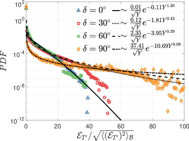
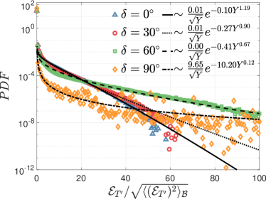
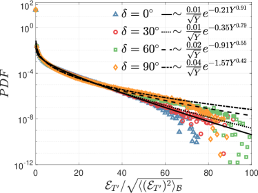
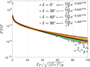
Figure 11: The PDFs of $\epsilon_{T^{\prime}}$ with different $\delta$ and $Ra$. The first line, from left to right: $Ra=3\times 10^{6}$, $Ra=3\times 10^{7}$. The second line, from left to right: $Ra=3\times 10^{8}$, $Ra=3\times 10^{9}$.

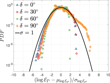
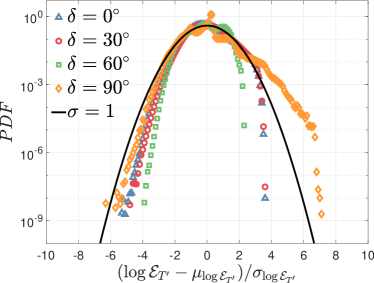
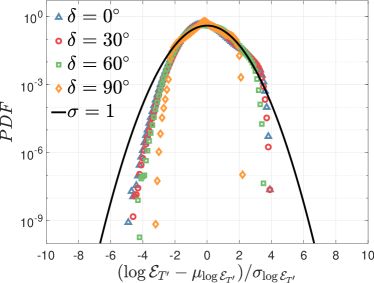
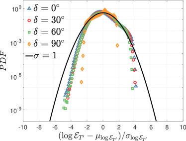
Figure 12: The PDFs of $\log\epsilon_{T^{\prime}}$ with different $\delta$ and $Ra$ The first line, from left to right: $Ra=3\times 10^{6}$, $Ra=3\times 10^{7}$. The second line, from left to right: $Ra=3\times 10^{8}$, $Ra=3\times 10^{9}$.

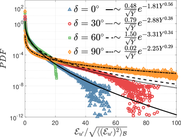
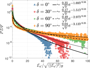
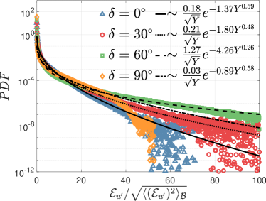
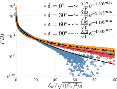
Figure 13: The PDFs of $\epsilon_{u^{\prime}}$ with different $\delta$ and $Ra$. The first line, from left to right: $Ra=3\times 10^{6}$, $Ra=3\times 10^{7}$. The second line, from left to right: $Ra=3\times 10^{8}$, $Ra=3\times 10^{9}$.

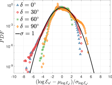
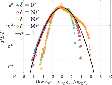
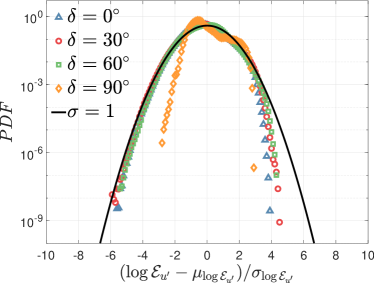
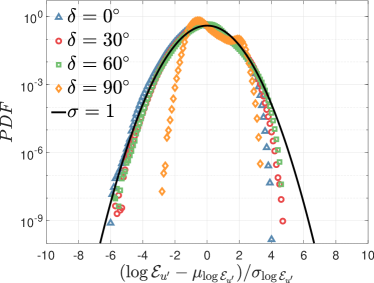
Figure 14: The PDFs of $\log\epsilon_{u^{\prime}}$ with different $\delta$ and $Ra$. The first line, from left to right: $Ra=3\times 10^{6}$, $Ra=3\times 10^{7}$. The second line, from left to right: $Ra=3\times 10^{8}$, $Ra=3\times 10^{9}$.

Next, we consider the effect of $\delta$ on the PDFs of the dissipation. The PDFs of $\epsilon_{T^{\prime}}$ for different $\delta$ are shown in figure 11 for $Ra=3\times 10^{6}$, $Ra=3\times 10^{7}$, $Ra=3\times 10^{8}$ and $Ra=3\times 10^{9}$. The results show that increasing $\delta$ has a dramatic effect on the PDFs. For $Ra=3\times 10^{6}$, $\alpha$ decreases monotonically as $\delta$ increases, indicating that the tails of the PDFs are decaying more slowly. This enhanced intermittency is because as $\delta$ is increased, the turbulence becomes localized to the lower edge of the bubble, and hence while in this region there is turbulence and dissipation, over vast portions of the bubble, the flow is almost quiescent.

As $Ra$ is increased, the impact of increasing $\delta$ on the PDFs of $\epsilon_{T^{\prime}}$ becomes much less dramatic, with $\alpha$ still decreasing with increasing $\delta$, but the effect of $\delta$ on $\alpha$ becoming much weaker as $Ra$ is increased. Indeed, the effect of tilt on the PDFs is quite weak for $Ra=3\times 10^{9}$. This reduced effect of $\delta$ as $Ra$ is increased is because with larger $Ra$, the turbulence produced at the lower edge of the bubble is sill vigorous and dominates the behavior of $\epsilon_{T^{\prime}}$, in contrast to the case of lower $Ra$ where the turbulence at the lower edge is strongly suppressed as $\delta$ is increased.

Figure 12 shows the PDFs of the logarithm of $\epsilon_{T^{\prime}}$ in normalized form, with a Gaussian distribution plotted as a solid black line for reference. Once again, we see that the deviation of the logarithmic PDFs from the Gaussian distribution is enhanced as $\delta$ is increased, but thus enhancement becomes weaker as $Ra$ increases. Plotting the PDFs in this form also helps reveal a significant difference between the DPR and SPR, namely, that while the logarithmic PDF is approximately Gaussian for small fluctuations of the dissipation in the DPR, it is far from a Gaussian in the SPR even for small fluctuations. Moreover, the results show that for $\delta=90^{\circ}$, the logarithmic PDF has a right tail that is heavier than a Guassian for the lower $Ra$ cases, but becomes lighter than a Guassian as $Ra$ increases. Moreover, for $Ra=3\times 10^{8}$ and $Ra=3\times 10^{9}$, the PDFs are weakly dependent on $\delta$ for $\delta\leq 60^{\circ}$.

The PDFs of $\epsilon_{u^{\prime}}$ are plotted in figure 13 for different $\delta$ and fixed $Ra$. These PDFs are again well described by stretched exponential functions, as was the case for the PDFs of $\epsilon_{T^{\prime}}$. The most striking difference compared to the PDFs of $\epsilon_{T^{\prime}}$ are that the PDFs of $\epsilon_{u^{\prime}}$ are much more sentitive to $\delta$, and remain sensitive to $\delta$ even for the largest $Ra$ considered. This difference can also be observed by considering the normalized PDFs of the logarithm of $\log\epsilon_{u^{\prime}}$ which are shown in figure 14. As with the normalized PDFs of the logarithm of $\log\epsilon_{T^{\prime}}$, those of $\log\epsilon_{u^{\prime}}$ shown in figure 14 show clear differences depending on whether the flow is in the DPR or the SPR. While the logarithmic PDF is approximately Gaussian for small fluctuations of the dissipation in the DPR, it is far from a Gaussian in the SPR even for small fluctuations. Indeed, for $Ra=3\times 10^{8}$ and $Ra=3\times 10^{9}$ the PDF for $\delta=90^{\circ}$ becomes bi-modal. The results also show that for $\delta=90^{\circ}$, the logarithmic PDF has a right tail that is heavier than a Guassian for the lower $Ra$ cases, but becomes lighter than a Guassian as $Ra$ increases.

IV.4 The Global Dissipation Scaling Rules

Having considered the PDFs of the dissipation rates, which quantify the local fluctuations of the dissipation rates in the flow, we now turn to consider the globally averaged dissipation rates, both due to the mean-fields and due to the fluctuating fields.

The globally averaged thermal and kinetic energy dissipation rates due to the mean-fields are denoted by $\langle\epsilon_{\langle T\rangle}\rangle_{\mathcal{B}}$ and $\langle\epsilon_{\langle u\rangle}\rangle_{\mathcal{B}}$. Figures 15 and 16 show $\langle\epsilon_{\langle T\rangle}\rangle_{\mathcal{B}}$ and $\langle\epsilon_{\langle u\rangle}\rangle_{\mathcal{B}}$ as function of $Ra$ for different $\delta$, with power-law fits illustrated by solid or dash lines. It is interesting that while the results show that $\langle\epsilon_{\langle T\rangle}\rangle_{\mathcal{B}}$ decreases with increasing $\delta$, $\langle\epsilon_{\langle u\rangle}\rangle_{\mathcal{B}}$ increases strongly with increasing $\delta$. This is due to the fact that as $\delta$ increases, the stable plume that dominates in the SPR creates two symmetric vortices, and these enhance the mean-shear in the flow.

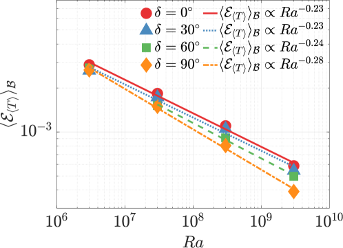
Figure 15: The variation of $\langle\epsilon_{\langle T\rangle}\rangle_{\mathcal{B}}$ with $Ra$ and $\delta$

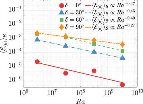
Figure 16: The variation of $\langle\epsilon_{\langle u\rangle}\rangle_{\mathcal{B}}$ with $Ra$ and $\delta$

Power-law fits to the data yield a scaling law of $\langle\epsilon_{\langle T\rangle}\rangle_{\mathcal{B}}\propto Ra^{-0.23}$ in the DPR and $\langle\epsilon_{\langle T\rangle}\rangle_{\mathcal{B}}\propto Ra^{-0.28}$ in the SPR. For $\langle\epsilon_{\langle u\rangle}\rangle_{\mathcal{B}}$, when $\delta=0^{\circ}$ the mean flow field is very weak, and $\langle\epsilon_{\langle u\rangle}\rangle_{\mathcal{B}}\propto Ra^{-0.47}$ is found, but the fitting errors are considerable. When $\delta=30^{\circ}$ and the flow is still in the DPR, the scaling law becomes $\langle\epsilon_{\langle u\rangle}\rangle_{\mathcal{B}}\propto Ra^{-0.43}$ with small negligible fitting error. The scaling law turns into $\langle\epsilon_{\langle u\rangle}\rangle_{\mathcal{B}}\propto Ra^{-0.49}$ for $\delta=60^{\circ}$ in the DPR. In the SPR, the behavior becomes $\langle\epsilon_{\langle u\rangle}\rangle_{\mathcal{B}}\propto Ra^{-0.27}$. The differing scaling behaviour of $\langle\epsilon_{\langle T\rangle}\rangle_{\mathcal{B}}$ and $\langle\epsilon_{\langle u\rangle}\rangle_{\mathcal{B}}$ in the DPR and SPR provide further evidence of the quantitative differences in the flow in these two distinct regimes.

Finally, we consider the globally averaged turbulent thermal and kinetic energy dissipation rates which are denoted by $\langle\epsilon_{T^{\prime}}\rangle_{\mathcal{B}}$ and $\langle\epsilon_{u^{\prime}}\rangle_{\mathcal{B}}$.

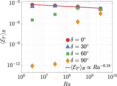
Figure 17: The variation of $\langle\epsilon_{T^{\prime}}\rangle_{\mathcal{B}}$ with $Ra$ and $\delta$

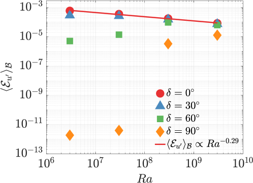
Figure 18: The variation of $\langle\epsilon_{u^{\prime}}\rangle_{\mathcal{B}}$ with $Ra$ and $\delta$

Figures 17 and 18 show $\langle\epsilon_{T^{\prime}}\rangle_{\mathcal{B}}$ and $\langle\epsilon_{u^{\prime}}\rangle_{\mathcal{B}}$ plotted as a function of $Ra$ for different $\delta$. The data shows an enormous influence of $\delta$ at lower $Ra$, which gradually reduces as $Ra$ is increased. More particularly, $\langle\epsilon_{T^{\prime}}\rangle_{\mathcal{B}}$ and $\langle\epsilon_{u^{\prime}}\rangle_{\mathcal{B}}$ dramatically reduce as $\delta$ is increased when $Ra$ is relatively small, e.g. $Ra=3\times 10^{6}$ and $Ra=3\times 10^{7}$, due to the strong suppression of convection and turbulence due to the tilting of the bubble. For relatively large $Ra$, e.g. $Ra=3\times 10^{8}$ and $Ra=3\times 10^{9}$, the reduction of $\langle\epsilon_{T^{\prime}}\rangle_{\mathcal{B}}$ and $\langle\epsilon_{u^{\prime}}\rangle_{\mathcal{B}}$ due to increasing $\delta$ are smaller, but still considerable. When the flow is in DPR, the scaling behaviours of $\langle\epsilon_{T^{\prime}}\rangle_{\mathcal{B}}$ and $\langle\epsilon_{u^{\prime}}\rangle_{\mathcal{B}}$ are $\langle\epsilon_{T^{\prime}}\rangle_{\mathcal{B}}\propto Ra^{-0.18}$ and $\langle\epsilon_{u^{\prime}}\rangle_{\mathcal{B}}\propto Ra^{-0.29}$. In contrast, the scaling of $\langle\epsilon_{T^{\prime}}\rangle_{\mathcal{B}}$ and $\langle\epsilon_{u^{\prime}}\rangle_{\mathcal{B}}$ in the SPR cannot be described by a power-law function that spans over the range of $Ra$ considered. This is another quantitative difference between the behavior of the flow in the DPR and SPR.

V Conclusion

In this paper, we have used DNS to explore the effect of tilt on the turbulent thermal convection taking place on a bubble. Visualizations of the flow reveal that as the tile angle $\delta$ is varied, the flow patterns fall into one of two regimes. When $\delta$ is relatively small, the flow is dominated by dynamic plumes that detach from the boundary layer at random locations on the equator. Turbulent thermal convection occurs on the bubble, associated with the continual generation and dissipation of these plumes. This flow pattern is referred to as the dynamic plume regime (DPR). On the other hand, when $\delta$ becomes sufficiently large, a single, large stable plume prevails on the bubble, emanating from the lower edge of the bubble. The stable large plume arises from an essentially fixed location on the equator and is persistent in time. This flow pattern is referred to as the stable plume regime (SPR). These qualitatively different flow regimes arise due to the geometric effect that tilting the bubble has on the direction of the local buoyancy force that drives the flow, and the way in which this depends upon location on the bubble surface.

The first quantitative difference between two regimes explored concerns the scaling behaviours of $Nu$ and $Re$. Concerning $Nu$, our result shows $Nu\propto Ra^{0.3}$ in the DPR, with a weak dependency of the exponent on $Ra$ and $\delta$. In the SPR, the scaling changes significantly and becomes $Nu\propto Ra^{0.24}$. For $Re$, the scaling in the DPR lies between $Re\propto Ra^{0.48}$ and $Re\propto Ra^{0.53}$ depending on $Ra$ and $\delta$, while in the SPR, the scaling lies between $Re\propto Ra^{0.44}$ and $Re\propto Ra^{0.45}$.

We then explored the behavior of the thermal and kinetic energy dissipation rates in the flow. The standardized PDFs of $\log\epsilon_{T^{\prime}}$ and $\log\epsilon_{u^{\prime}}$ have very different shapes in the DPR and SPR. For $\log\epsilon_{T^{\prime}}$ and $\log\epsilon_{u^{\prime}}$, the shape of the PDFs are close to a Guassian PDFs for small values, but deviates from it for large values in the DPR. In the SPR, the PDFs of $\log\epsilon_{T^{\prime}}$ and $\log\epsilon_{u^{\prime}}$ depart considerably from a Gaussian PDF for both small and large values, and the PDF of $\log\epsilon_{u^{\prime}}$ has a bi-modal shape at small values.

The globally averaged thermal energy dissipation rate due to the mean temperature field was shown to exhibit the scaling $\langle\epsilon_{\langle T\rangle}\rangle_{\mathcal{B}}\propto Ra^{-0.23}$ in the DPR, and $\langle\epsilon_{\langle T\rangle}\rangle_{\mathcal{B}}\propto Ra^{-0.28}$ in the SPR. The globally averaged kinetic energy dissipation rate due to the mean velocity field was shown to exhibit the scaling $\langle\epsilon_{\langle u\rangle}\rangle_{\mathcal{B}}\propto Ra^{-0.47}$ in the DPR (the exponent reduces from $0.47$ to $0.43$ as $\delta$ is increased up to $30^{\circ}$). In the SPR, the behavior changes considerably to $\langle\epsilon_{\langle u\rangle}\rangle_{\mathcal{B}}\propto Ra^{-0.27}$. For the turbulent dissipation rates, the results indicate the scaling $\langle\epsilon_{T^{\prime}}\rangle_{\mathcal{B}}\propto Ra^{-0.18}$ and $\langle\epsilon_{u^{\prime}}\rangle_{\mathcal{B}}\propto Ra^{-0.29}$ in the DPR. However, the dependencies of $\langle\epsilon_{T^{\prime}}\rangle_{\mathcal{B}}$ and $\langle\epsilon_{u^{\prime}}\rangle_{\mathcal{B}}$ on $Ra$ cannot be described by power-laws in the SPR.

Taken together, these results show that the two-dimensional flow on the half-soap bubble undergoes dramatic changes, both qualitative and quantitative, as the bubble is tilted relative to the direction of gravity. This has significant impacts for understanding convective flows in natural and engineered contexts where mean temperature gradients in the flow are often not aligned with gravity, and where the flow may take place on (or in) curved geometries.

References

- Lohse and Xia (2010) D. Lohse and K.-Q. Xia, “Small-scale properties of turbulent rayleigh-bénard convection,” Annual Review of Fluid Mechanics 42, 335–364 (2010).
- Guo et al. (2022) X.-Q. Guo, B.-F. Wang, J.-Z. Wu, K. L. Chong, and Q. Zhou, “Turbulent vertical convection under vertical vibration,” Physics of Fluids 34, 055106 (2022), 10.1063/5.0090250 .
- Ahlers, Grossmann, and Lohse (2009) G. Ahlers, S. Grossmann, and D. Lohse, “Heat transfer and large scale dynamics in turbulent rayleigh-bénard convection,” Reviews of Modern Physics 81, 503–537 (2009).
- Xu, Shi, and Xi (2019) A. Xu, L. Shi, and H.-D. Xi, “Statistics of temperature and thermal energy dissipation rate in low-prandtl number turbulent thermal convection,” Physics of Fluids 31, 125101 (2019), 10.1063/1.5129818 .
- He, Ching, and Tong (2011) X. He, E. S. C. Ching, and P. Tong, “Locally averaged thermal dissipation rate in turbulent thermal convection: A decomposition into contributions from different temperature gradient components,” Physics of Fluids 23, 025106 (2011), 10.1063/1.3555637 .
- Petschel et al. (2015) K. Petschel, S. Stellmach, M. Wilczek, J. Lülff, and U. Hansen, “Kinetic energy transport in rayleigh–bénard convection,” Journal of Fluid Mechanics 773, 395–417 (2015).
- Petschel et al. (2013) K. Petschel, S. Stellmach, M. Wilczek, J. Lülff, and U. Hansen, “Dissipation layers in rayleigh-bénard convection: A unifying view,” Phys. Rev. Lett. 110, 114502 (2013).
- Zhang, Zhou, and Sun (2017) Y. Zhang, Q. Zhou, and C. Sun, “Statistics of kinetic and thermal energy dissipation rates in two-dimensional turbulent rayleigh–bénard convection,” Journal of Fluid Mechanics 814, 165–184 (2017).
- Hertlein and du Puits (2021) A. Hertlein and R. du Puits, “Direct measurements of the thermal dissipation rate in turbulent rayleigh–bénard convection,” Physics of Fluids 33, 035139 (2021), 10.1063/5.0033746 .
- Stevens, Clercx, and Lohse (2013) R. J. Stevens, H. J. Clercx, and D. Lohse, “Heat transport and flow structure in rotating rayleigh–bénard convection,” European Journal of Mechanics - B/Fluids 40, 41–49 (2013), fascinating Fluid Mechanics: 100-Year Anniversary of the Institute of Aerodynamics, RWTH Aachen University.
- Shraiman and Siggia (1990) B. I. Shraiman and E. D. Siggia, “Heat transport in high-rayleigh-number convection,” Phys. Rev. A 42, 3650–3653 (1990).
- Siggia (1994) E. D. Siggia, “High rayleigh number convection,” Annual Review of Fluid Mechanics 26, 137–168 (1994), 10.1146/annurev.fl.26.010194.001033 .
- Grossmann and Lohse (2000) S. Grossmann and D. Lohse, “Scaling in thermal convection: a unifying theory,” Journal of Fluid Mechanics 407, 27–56 (2000).
- Grossmann and Lohse (2001) S. Grossmann and D. Lohse, “Thermal convection for large prandtl numbers,” Phys. Rev. Lett. 86, 3316–3319 (2001).
- Grossmann and Lohse (2002) S. Grossmann and D. Lohse, “Prandtl and rayleigh number dependence of the reynolds number in turbulent thermal convection,” Phys. Rev. E 66, 016305 (2002).
- Grossmann and Lohse (2004) S. Grossmann and D. Lohse, “Fluctuations in turbulent rayleigh–bénard convection: The role of plumes,” Physics of Fluids 16, 4462–4472 (2004), https://doi.org/10.1063/1.1807751 .
- He and Tong (2009) X. He and P. Tong, “Measurements of the thermal dissipation field in turbulent rayleigh-bénard convection,” Phys. Rev. E 79, 026306 (2009).
- He, Tong, and Xia (2007) X. He, P. Tong, and K.-Q. Xia, “Measured thermal dissipation field in turbulent rayleigh-bénard convection,” Phys. Rev. Lett. 98, 144501 (2007).
- Ni, Huang, and Xia (2011) R. Ni, S.-D. Huang, and K.-Q. Xia, “Local energy dissipation rate balances local heat flux in the center of turbulent thermal convection,” Phys. Rev. Lett. 107, 174503 (2011).
- Méthivier et al. (2022) L. Méthivier, R. Braun, F. Chillà, and J. Salort, “Turbulent transition in rayleigh-bénard convection with fluorocarbon (a),” Europhysics Letters 136, 10003 (2022).
- Verzicco and Camussi (2003) R. Verzicco and R. Camussi, “Numerical experiments on strongly turbulent thermal convection in a slender cylindrical cell,” Journal of Fluid Mechanics 477, 19–49 (2003).
- Verzicco (2003) R. Verzicco, “Turbulent thermal convection in a closed domain: viscous boundary layer and mean flow effects,” The European Physical Journal B-Condensed Matter and Complex Systems 35, 133–141 (2003).
- Shishkina and Wagner (2006) O. Shishkina and C. Wagner, “Analysis of thermal dissipation rates in turbulent rayleigh–bénard convection,” Journal of Fluid Mechanics 546, 51–60 (2006).
- Shishkina and Wagner (2007) O. Shishkina and C. Wagner, “Local heat fluxes in turbulent rayleigh-bénard convection,” Physics of Fluids 19, 085107 (2007).
- Shishkina and Wagner (2008) O. Shishkina and C. Wagner, “Analysis of sheet-like thermal plumes in turbulent rayleigh–bénard convection,” Journal of Fluid Mechanics 599, 383–404 (2008).
- Emran and Schumacher (2008) M. S. Emran and J. Schumacher, “Fine-scale statistics of temperature and its derivatives in convective turbulence,” Journal of Fluid Mechanics 611, 13–34 (2008).
- Bhattacharya, Samtaney, and Verma (2019) S. Bhattacharya, R. Samtaney, and M. K. Verma, “Scaling and spatial intermittency of thermal dissipation in turbulent convection,” Physics of Fluids 31, 075104 (2019), 10.1063/1.5098073 .
- Hideo (1984) I. Hideo, “Experimental study of natural convection in an inclined air layer,” International Journal of Heat and Mass Transfer 27, 1127–1139 (1984).
- Bejan (2013) A. Bejan, Convection heat transfer (John wiley & sons, 2013).
- Taylor and McLennan (1995) S. R. Taylor and S. M. McLennan, “The geochemical evolution of the continental crust,” Reviews of Geophysics 33 (1995), 10.1029/95rg00262.
- Wortel and Spakman (2000) M. J. Wortel and W. Spakman, “Subduction and slab detachment in the mediterranean-carpathian region,” Science 290, 1910–7 (2000).
- Condie (2008) K. C. Condie, “Mantle plumes: A multidisciplinary approach,” Eos, Transactions American Geophysical Union 89 (2008), 10.1029/2008eo110011.
- Emanuel, David Neelin, and Bretherton (1994) K. A. Emanuel, J. David Neelin, and C. S. Bretherton, “On large-scale circulations in convecting atmospheres,” Quarterly Journal of the Royal Meteorological Society 120, 1111–1143 (1994).
- Madanan and Goldstein (2019) U. Madanan and R. J. Goldstein, “Experimental investigation on very-high-rayleigh-number thermal convection in tilted rectangular enclosures,” International Journal of Heat and Mass Transfer 139, 121–129 (2019).
- Ahlers, Brown, and Nikolaenko (2006) G. Ahlers, E. Brown, and A. Nikolaenko, “The search for slow transients, and the effect of imperfect vertical alignment, in turbulent rayleigh–bénard convection,” Journal of Fluid Mechanics 557 (2006), 10.1017/s0022112006009888.
- Guo et al. (2015) S.-X. Guo, S.-Q. Zhou, X.-R. Cen, L. Qu, Y.-Z. Lu, L. Sun, and X.-D. Shang, “The effect of cell tilting on turbulent thermal convection in a rectangular cell,” Journal of Fluid Mechanics 762, 273–287 (2015).
- Wang et al. (2018a) Q. Wang, Z.-H. Wan, R. Yan, and D.-J. Sun, “Multiple states and heat transfer in two-dimensional tilted convection with large aspect ratios,” Physical Review Fluids 3 (2018a), 10.1103/PhysRevFluids.3.113503.
- Wang et al. (2018b) Q. Wang, S.-N. Xia, B.-F. Wang, D.-J. Sun, Q. Zhou, and Z.-H. Wan, “Flow reversals in two-dimensional thermal convection in tilted cells,” Journal of Fluid Mechanics 849, 355–372 (2018b).
- Wei and Xia (2013) P. Wei and K.-Q. Xia, “Viscous boundary layer properties in turbulent thermal convection in a cylindrical cell: the effect of cell tilting,” Journal of Fluid Mechanics 720, 140–168 (2013).
- Shishkina and Horn (2016) O. Shishkina and S. Horn, “Thermal convection in inclined cylindrical containers,” Journal of Fluid Mechanics 790 (2016), 10.1017/jfm.2016.55.
- Zwirner and Shishkina (2018) L. Zwirner and O. Shishkina, “Confined inclined thermal convection in low-prandtl-number fluids,” Journal of Fluid Mechanics 850, 984–1008 (2018).
- Zhang, Ding, and Xia (2021) L. Zhang, G.-Y. Ding, and K.-Q. Xia, “On the effective horizontal buoyancy in turbulent thermal convection generated by cell tilting,” Journal of Fluid Mechanics 914 (2021), 10.1017/jfm.2020.825.
- Kellay (2017) H. Kellay, “Hydrodynamics experiments with soap films and soap bubbles: A short review of recent experiments,” Physics of fluids 29, 111113 (2017).
- Kellay and Goldburg (2002) H. Kellay and W. I. Goldburg, “Two-dimensional turbulence: a review of some recent experiments,” Reports on Progress in Physics 65, 845–894 (2002).
- Seychelles et al. (2008) F. Seychelles, Y. Amarouchene, M. Bessafi, and H. Kellay, “Thermal convection and emergence of isolated vortices in soap bubbles,” Physical review letters 100, 144501 (2008).
- Seychelles et al. (2010) F. Seychelles, F. Ingremeau, C. Pradere, and H. Kellay, “From intermittent to nonintermittent behavior in two dimensional thermal convection in a soap bubble,” Physical review letters 105, 264502 (2010).
- Meuel et al. (2018) T. Meuel, M. Coudert, P. Fischer, C. H. Bruneau, and H. Kellay, “Effects of rotation on temperature fluctuations in turbulent thermal convection on a hemisphere,” Scientific Reports 8 (2018), 10.1038/s41598-018-34782-0.
- Meuel et al. (2012) T. Meuel, G. Prado, F. Seychelles, M. Bessafi, and H. Kellay, “Hurricane track forecast cones from fluctuations,” Scientific reports 2, 1–8 (2012).
- Meuel et al. (2013) T. Meuel, Y. L. Xiong, P. Fischer, C. H. Bruneau, M. Bessafi, and H. Kellay, “Intensity of vortices: from soap bubbles to hurricanes,” Scientific Reports 3 (2013), 10.1038/srep03455.
- Xiong, Fischer, and Bruneau (2012) Y. L. Xiong, P. Fischer, and C.-H. Bruneau, “Numerical simulations of two-dimensional turbulent thermal convection on the surface of a soap bubble,” Proc ICCFD 7, 3703 (2012).
- Bruneau et al. (2018) C. H. Bruneau, P. Fischer, Y. L. Xiong, and H. Kellay, “Numerical simulations of thermal convection on a hemisphere,” Physical Review Fluids 3 (2018), 10.1103/PhysRevFluids.3.043502.
- He et al. (2021) X. He, A. Bragg, Y. Xiong, and P. Fischer, “Turbulence and heat transfer on a rotating, heated half soap bubble,” Journal of Fluid Mechanics 924, A19 (2021).
- Boffetta and Ecke (2012) G. Boffetta and R. E. Ecke, “Two-dimensional turbulence,” Annual Review of Fluid Mechanics 44, 427–451 (2012), 10.1146/annurev-fluid-120710-101240 .
- Sun and Xia (2005) C. Sun and K.-Q. Xia, “Scaling of the reynolds number in turbulent thermal convection,” Physical review. E, Statistical, nonlinear, and soft matter physics 72, 067302 (2005).
- Chertkov, Falkovich, and Kolokolov (1998) M. Chertkov, G. Falkovich, and I. Kolokolov, “Intermittent dissipation of a passive scalar in turbulence,” Phys. Rev. Lett. 80, 2121–2124 (1998).
- Kaczorowski and Wagner (2009) M. Kaczorowski and C. Wagner, “Analysis of the thermal plumes in turbulent rayleigh–bénard convection based on well-resolved numerical simulations,” Journal of Fluid Mechanics 618, 89–112 (2009).