Anticoncentration in Ramsey graphs and a proof of the Erdős–McKay conjecture

Abstract.

An $n$-vertex graph is called $C$-Ramsey if it has no clique or independent set of size $C\log_{2}n$ (i.e., if it has near-optimal Ramsey behavior). In this paper, we study edge-statistics in Ramsey graphs, in particular obtaining very precise control of the distribution of the number of edges in a random vertex subset of a $C$-Ramsey graph. This brings together two ongoing lines of research: the study of “random-like” properties of Ramsey graphs and the study of small-ball probabilities for low-degree polynomials of independent random variables.

The proof proceeds via an “additive structure” dichotomy on the degree sequence, and involves a wide range of different tools from Fourier analysis, random matrix theory, the theory of Boolean functions, probabilistic combinatorics, and low-rank approximation. One of the consequences of our result is the resolution of an old conjecture of Erdős and McKay, for which Erdős offered one of his notorious monetary prizes.

1. Introduction

An induced subgraph of a graph is called homogeneous if it is a clique or independent set (i.e., all possible edges are present, or none are). One of the most fundamental results in Ramsey theory, proved in 1935 by Erdős and Szekeres [35], states that every $n$-vertex graph contains a homogeneous subgraph with at least $\frac{1}{2}\log_{2}n$ vertices. On the other hand, Erdős [30] famously used the probabilistic method to prove that, for all $n\geq 3$, there is an $n$-vertex graph with no homogeneous subgraph on $2\log_{2}n$ vertices. Despite significant effort (see for example [11, 68, 17, 44, 21, 18, 72, 1, 45, 49]), there are no known non-probabilistic constructions of graphs with comparably small homogeneous sets, and in fact the problem of explicitly constructing such graphs is intimately related to randomness extraction in theoretical computer science (see for example [86] for an introduction to the topic).

For some $C>0$, an $n$-vertex graph is called $C$-Ramsey if it has no homogeneous subgraph of size $C\log_{2}n$. We think of $C$ as being a constant (not varying with $n$), so $C$-Ramsey graphs are those graphs with near-optimal Ramsey behavior. It is widely believed that $C$-Ramsey graphs must in some sense resemble random graphs (which would provide some explanation for why it is so hard to find explicit constructions), and this belief has been supported by a number of theorems showing that certain structural or statistical properties characteristic of random graphs hold for all $C$-Ramsey graphs. The first result of this type was due to Erdős and Szemerédi [36], who showed that every $C$-Ramsey graph $G$ has edge-density bounded away from zero and one (formally, for any $C>0$ there is $\varepsilon_{C}>0$ such that for sufficiently large $n$, the number of edges in any $C$-Ramsey graph with $n$ vertices lies between $\varepsilon_{C}\binom{n}{2}$ and $(1-\varepsilon_{C})\binom{n}{2}$). Note that this implies fairly strong information about the edge distribution on induced subgraphs of $G$, because any induced subgraph of $G$ with at least $n^{\alpha}$ vertices is itself $(C/\alpha)$-Ramsey.

This basic result was the foundation for a large amount of further research on Ramsey graphs; over the years many conjectures have been proposed and many theorems proved (see for example [2, 3, 4, 7, 8, 14, 34, 31, 57, 63, 64, 73, 81, 87, 9, 67]). Particular attention has focused on a sequence of conjectures made by Erdős and his collaborators, exploring the theme that Ramsey graphs must have diverse induced subgraphs. For example, for a $C$-Ramsey graph $G$ with $n$ vertices, it was proved by Prömel and Rödl [81] (answering a conjecture of Erdős and Hajnal) that $G$ contains every possible induced subgraph on $\delta_{C}\log n$ vertices; by Shelah [87] (answering a conjecture of Erdős and Rényi) that $G$ contains $2^{\delta_{C}n}$ non-isomorphic induced subgraphs; by the first author and Sudakov [63] (answering a conjecture of Erdős, Faudree, and Sós) that $G$ contains $\delta_{C}n^{5/2}$ subgraphs that can be distinguished by looking at their edge and vertex numbers; and by Jenssen, Keevash, Long, and Yepremyan [57] (improving on a conjecture of Erdős, Faudree, and Sós proved by Bukh and Sudakov [14]) that $G$ contains an induced subgraph with $\delta_{C}n^{2/3}$ distinct degrees (all for some $\delta_{C}>0$ depending on $C$).

Only one of Erdős’ conjectures (on properties of $C$-Ramsey graphs) from this period has remained open until now: Erdős and McKay (see [31]) made the ambitious conjecture that for essentially any “sensible” integer $x$, every $C$-Ramsey graph must necessarily contain an induced subgraph with exactly $x$ edges. To be precise, they conjectured that there is $\delta_{C}>0$ depending on $C$ such that for any $C$-Ramsey graph $G$ with $n$ vertices and any integer $0\leq x\leq\delta_{C}n^{2}$, there is an induced subgraph of $G$ with exactly $x$ edges. Erdős reiterated this problem in several collections of his favorite open problems in combinatorics [31, 32] (also in [33]), and offered one of his notorious monetary prizes ($100) for its solution (see [32, 20, 19]).

Progress on the Erdős–McKay conjecture has come from four different directions. First, the canonical example of a Ramsey graph is (a typical outcome of) an Erdős–Rényi random graph. It was proved by Calkin, Frieze and McKay [15] (answering questions raised by Erdős and McKay) that for any constants $p\in(0,1)$ and $\eta>0$, a random graph $\mathbb{G}(n,p)$ typically contains induced subgraphs with all numbers of edges up to $(1-\eta)p\binom{n}{2}$. Second, improving on initial bounds of Erdős and McKay [31], it was proved by Alon, Krivelevich, and Sudakov [8] that there is $\alpha_{C}>0$ such that in a $C$-Ramsey graph on $n$ vertices, one can always find an induced subgraph with any given number of edges up to $n^{\alpha_{C}}$. Third, improving on a result of Narayanan, Sahasrabudhe, and Tomon [73], the first author and Sudakov [64] proved that there is $\delta_{C}>0$ such that in any $C$-Ramsey graph on $n$ vertices contains induced subgraphs with $\delta_{C}n^{2}$ different numbers of edges (though without making any guarantee on what those numbers of edges are). Finally, Long and Ploscaru [69] recently proved a bipartite analog of the Erdős–McKay conjecture.

As our first result, we prove a substantial strengthening of the Erdős–McKay conjecture. Let $e(G)$ be the number of edges in a graph $G$.

Theorem 1.1.

Fix $C>0$ and $\eta>0$, and let $G$ be a $C$-Ramsey graph on $n$ vertices, where $n$ is sufficiently large with respect to $C$ and $\eta$. Then for any integer $x$ with $0\leq x\leq(1-\eta)e(G)$, there is a subset $U\subseteq V(G)$ inducing exactly $x$ edges.

Given prior results due to Alon, Krivelevich and Sudakov [8], Theorem 1.1 is actually a simple corollary of a much deeper result (Theorem 1.2) on edge-statistics in Ramsey graphs, which we discuss in the next subsection.

1.1. Edge-statistics and low-degree polynomials

For an $n$-vertex graph $G$, observe that the number of edges $e(G[U])$ in an induced subgraph $G[U]$ can be viewed as an evaluation of a quadratic polynomial associated with $G$. Indeed, identifying the vertex set of $G$ with $\{1,\ldots,n\}$ and writing $E$ for the edge set of $G$, consider the $n$-variable quadratic polynomial $f(\xi_{1},\ldots,\xi_{n})=\sum_{ij\in E}\xi_{i}\xi_{j}$. Then, for any vertex set $U$, let $\vec{\xi}\,^{(U)}$ be the characteristic vector of $U$ (with $\vec{\xi}\,^{(U)}_{v}=1$ if $v\in U$, and $\vec{\xi}\,^{(U)}_{v}=0$ if $v\notin U$). It is easy to check that the number of edges $e(G[U])$ induced by $U$ is precisely equal to $f(\vec{\xi}\,^{(U)})$. That is, to say, the statement that $G$ has an induced subgraph with exactly $x$ edges is precisely equivalent to the statement that there is a binary vector $\vec{\xi}\in\{0,1\}^{n}$ with $f(\vec{\xi})=x$.

There are many combinatorial quantities of interest that can be interpreted as low-degree polynomials of binary vectors. For example, the number of triangles in a graph, or the number of 3-term arithmetic progressions in a set of integers, can both be naturally interpreted as evaluations of certain cubic polynomials. More generally, the study of Boolean functions is the study of functions of the form $f\colon\{0,1\}^{n}\to\mathbb{R}$; every such function can be written (uniquely) as a multilinear polynomial, and the degree of this polynomial is a fundamental measure of the “complexity” of the Boolean function.

One of the most important discoveries from the analysis of Boolean functions is that it is fruitful to study the behavior of (low-degree) Boolean functions evaluated on a random binary vector $\vec{\xi}\in\{0,1\}^{n}$. This is the perspective we take in this paper: as our main result, for any Ramsey graph $G$ and a random vertex subset $U$, we obtain very precise control over the distribution of $e(G[U])$.

Theorem 1.2.

Fix $C,\lambda>0$, let $G$ be a $C$-Ramsey graph on $n$ vertices and let $\lambda\leq p\leq 1-\lambda$. Then if $U$ is a random subset of $V(G)$ obtained by independently including each vertex with probability $p$, we have

$$\sup_{x\in\mathbb{Z}}\Pr[e(G[U])=x]\leq K_{C,\lambda}n^{-3/2}$$

for some $K_{C,\lambda}>0$ depending only on $C,\lambda$. Furthermore, for every fixed $A>0$, we have

$$\qquad\inf_{\begin{subarray}{c}x\in\mathbb{Z}\\ |x-p^{2}e(G)|\leq An^{3/2}\end{subarray}}\Pr[e(G[U])=x]\geq\kappa_{C,A,\lambda}n^{-3/2}$$

for some $\kappa_{C,A,\lambda}>0$ depending only on $C,A,\lambda$, if $n$ is sufficiently large in terms of $C,\lambda$ and $A$.

It is not hard to show that for any $C$-Ramsey graph $G$, the standard deviation $\sigma$ of $e(G[U])$ is of order $n^{3/2}$. So, Theorem 1.2 says (roughly speaking) that in the “bulk” of the distribution of $e(G[U])$ (i.e., within roughly standard-deviation-range of the mean), the point probabilities are all of order $1/\sigma$. In Section 2 we will give the short deduction of Theorem 1.1 from Theorem 1.2 and the aforementioned theorem of Alon, Krivelevich, and Sudakov.

Remark 1.3.

Our proof of Theorem 1.2 can be adapted to handle slightly more general types of graphs than Ramsey graphs. For example, we can obtain the same conclusions in the case where $G$ is a $d$-regular graph with $0.01n\leq d\leq 0.99n$, such that the eigenvalues $\lambda_{1}\geq\cdots\geq\lambda_{n}$ of the adjacency matrix of $G$ satisfy $\max\{\lambda_{2},-\lambda_{n}\}\leq n^{1/2+0.01}$ (i.e., the case where $G$ is a dense graph with near-optimal spectral expansion). See Remarks 4.5 and 4.2 for some discussion of the necessary adaptations. Notably, this class of graphs includes Paley graphs, which are “random-like” graphs with an explicit number-theoretic definition (see for example [60]). These graphs are currently one of the most promising candidates for explicit constructions of Ramsey graphs, though precisely studying the Ramsey properties of these graphs seems to be outside the reach of current techniques in number theory (see [53, 26] for recent developments).

Remark 1.4.

If $p=1/2$, then the random set $U$ in Theorem 1.2 is simply a uniformly random subset of vertices. So, for $x$ close to $e(G)/4$, Theorem 1.2 tells us that the number of induced subgraphs with $x$ edges is of order $2^{n}/n^{3/2}$. It would be interesting to investigate the number of $x$-edge induced subgraphs for general $x$ (not close to $e(G)/4$). From Theorem 1.2 one can deduce a lower bound on this number approximately matching the behavior of an appropriate Erdős–Rényi random graph (i.e., for any constant $\eta>0$, and $\eta n^{2}\leq x\leq(1-\eta)e(G)$, there are at least $\exp(H(\sqrt{x/e(G)})n+o(n))$ subgraphs with $x$ edges, where $H$ denotes the base-$e$ entropy function). However, a corresponding upper bound does not in general hold: to characterize the number of $x$-edge induced subgraphs up to any sub-exponential error term, one must incorporate more detailed information about the Ramsey graph $G$ than just its number of edges. (To see this, consider a union of two disjoint independent Erdős–Rényi random graphs $\mathbb{G}(n/2,0.01)\sqcup\mathbb{G}(n/2,0.99)$, and count subgraphs with $0.001n^{2}$ edges.)

There has actually been quite some recent interest (see for example [65, 41, 70, 42, 6]) studying random variables of the form $e(G[U])$ for a graph $G$ and a random vertex set $U$, largely due to a sequence of conjectures by Alon, Hefetz, Krivelevich, and Tyomkyn [6] motivated by the classical topic of graph inducibility. Specifically, these works studied the anticoncentration behavior of $e(G[U])$ (generally speaking, anticoncentration inequalities provide upper bounds on the probability that a random variable falls in some small ball or is equal to some particular value). As discussed above, $e(G[U])$ can be naturally interpreted as a quadratic polynomial, so this study falls within the scope of the so-called polynomial Littlewood–Offord problem (which concerns anticoncentration of general low-degree polynomials of various types of random variables). There has been a lot of work from several different directions (see for example [23, 58, 62, 89, 75, 52, 88, 84, 74, 76]) on the extent to which anticoncentration in the (polynomial) Littlewood–Offord problem is controlled by algebraic or arithmetic structure, and the upper bound in Theorem 1.2 can be viewed in this context: Ramsey graphs yield quadratic polynomials that are highly unstructured in a certain combinatorial sense, and we see that such polynomials have strong anticoncentration behavior.

The first author, Sudakov and Tran [65] previously suggested to study anticoncentration of $e(G[W])$ for a Ramsey graph $G$ and a random vertex subset $W$ of a given size. In particular, they asked whether for a $C$-Ramsey graph $G$ with $n$ vertices, and a uniformly random subset $W$ of exactly $n/2$ vertices, we have $\sup_{x\in\mathbb{Z}}\Pr[e(G[W])=x]\leq K_{C}/n$ for some $K_{C}>0$ depending only on $C$. Some progress was made on this question by the first and third authors [62]; as a simple corollary of Theorem 1.2, we answer this question in the affirmative.

Theorem 1.5.

For $C>0$ and $0<\lambda<1$, there is $K=K(C,\lambda)$ such that the following holds. Let $G$ be a $C$-Ramsey graph on $n$ vertices and let $W\subseteq V(G)$ be a random subset of exactly $k$ vertices, for some given $k$ with $\lambda n\leq k\leq(1-\lambda)n$. Then

$$\sup_{x\in\mathbb{Z}}\Pr[e(G[W])=x]\leq\frac{K}{n}.$$

It is not hard to show that the upper bound in Theorem 1.5 is best-possible (indeed, this can be seen by taking $G$ to be a typical outcome of an Erdős–Rényi random graph $\mathbb{G}(n,1/2)$). However, in contrast to the setting of Theorem 1.2, in Theorem 1.5 one cannot hope for a matching lower bound when $x$ is close to $\mathbb{E}[e(G[W])]$ (as can be seen by considering the case where $G$ is a typical outcome of the union of two disjoint independent Erdős–Rényi random graphs $\mathbb{G}(n,1/4)\sqcup\mathbb{G}(n,3/4)$).

1.2. Proof ingredients and ideas

We outline the proof of Theorem 1.2 in more detail in Section 3, but here we take the opportunity to highlight some of the most important ingredients and ideas.

1.2.1. An approximate local limit theorem

A starting point is that, in the setting of Theorem 1.2, standard techniques show that $e(G[U])$ satisfies a central limit theorem: we have $\Pr[e(G[U])\leq x]=\Phi((x-\mu)/\sigma)+o(1/\sigma)$ for all $x\in\mathbb{R}$, where $\Phi$ is the standard Gaussian cumulative distribution function, and $\mu,\sigma$ are the mean and standard deviation of $e(G[U])$. It is natural to wonder (as suggested in [62] as a potential path towards the Erdős–McKay conjecture) whether this can be strengthened to a local central limit theorem: could it be that for all $x\in\mathbb{R}$ we have $\Pr[e(G[U])=x]=\Phi^{\prime}((x-\mu)/\sigma)/\sigma+o(1/\sigma)$ (where $\Phi^{\prime}$ is the standard Gaussian density function)? In fact, the statement of Theorem 1.2 can be interpreted as a local central limit theorem “up to constant factors”. This perspective also suggests a strategy for the proof of Theorem 1.2: perhaps we can leverage Fourier-analytic techniques previously developed for local central limit theorems (e.g. [48, 91, 13, 12, 47, 61]), obtaining our desired result as a consequence of estimates on the characteristic function (i.e., Fourier transform) of our random variable $e(G[U])$.

However, it turns out that a local central limit theorem actually does not hold in general: while the coarse-scale distribution of $e(G[U])$ is always Gaussian, in general $e(G[U])$ may have a rather nontrivial “two-scale” behavior, depending on the additive structure of the degree sequence of $G$ (see Figure 1). Roughly speaking, this translates to a certain “spike” in the magnitude of the characteristic function of $e(G[U])$, which rules out naïve Fourier-analytic approaches. To overcome this issue, we need to capture the “reason” for the two-scale behavior: It turns out that this “spike” can only happen if the degree sequence of $G$ is in a certain sense “additively structured”, implying that there is a partition of the vertex set into “buckets” such that vertices in the same bucket have almost the same degree. Then, if we reveal the size of the intersection of $U$ with each bucket, the conditional characteristic function of $e(G[U])$ is suitably bounded. We deduce conditional bounds on the point probabilities of $e(G[U])$, and average these over possible outcomes of the revealed intersection sizes of $U$ with the buckets.

       

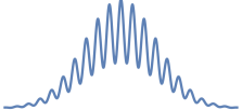
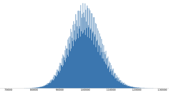
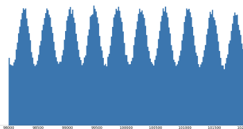
Figure 1. On the left is a cartoon of (one possibility for) the probability mass function of $e(G[U])$ for a Ramsey graph $G$ and a uniformly random vertex subset $U$: the large-scale behavior is Gaussian, but on a small scale we see many smaller Gaussian-like curves. The two images on the right are two different histograms at different scales, obtained from real data (namely, from two million independent samples of a uniformly random vertex subset in a graph $G$ obtained as an outcome of the Erdős–Rényi random graph $\mathbb{G}(1000,0.8)$).

We remark that one interpretation of our proof strategy is that we are decomposing our random variable into “components” in physical space, in such a way that each component is well-behaved in Fourier space. This is at least superficially reminiscent of certain techniques in harmonic analysis; see for example [51]. Looking beyond the particular statement of Theorem 1.2, we hope that the Fourier-analytic techniques in its proof will be useful for the general study of small-ball probabilities for low-degree polynomials of independent variables, especially in settings where Gaussian behavior may break down.

1.2.2. Small-ball probability for quadratic Gaussian chaos

The general study of low-degree polynomials of independent random variables (sometimes called chaoses) has a long and rich history. Some highlights include Kim–Vu polynomial concentration [59], the Hanson–Wright inequality [54], the Bonami–Beckner hypercontractive inequality (see [78]), and polynomial chaos expansion (see [46]), which are fundamental tools in probabilistic combinatorics, high-dimensional statistics, the analysis of Boolean functions and mathematical modelling.

Much of this study has focused on low-degree polynomials of Gaussian random variables, which enjoy certain symmetry properties that make them easier to study. While this direction may not seem obviously relevant to Theorem 1.2, in part of the proof we are able to apply the celebrated Gaussian invariance principle of Mossel, O’Donnell, and Oleszkiewicz [71], to compare our random variables of interest with certain “Gaussian analogs”. Therefore, a key step in the proof of Theorem 1.2 is to study small-ball probability for quadratic polynomials of Gaussian random variables.

The fundamental theorem in this area is the Carbery–Wright theorem [16], which (specialized to the quadratic case) says that for $0<\varepsilon<1$ and any real quadratic polynomial $f=f(Z_{1},\ldots,Z_{n})$ of independent standard Gaussian random variables $Z_{1},\ldots,Z_{n}\sim\mathcal{N}(0,1)$, we have

$$\sup_{x\in\mathbb{R}}\Pr[|f-x|\leq\varepsilon]=O(\sqrt{\varepsilon/\sigma(f)}).$$

This is best-possible in general (for example, $\Pr[|Z_{1}^{2}|\leq\varepsilon]$ scales like $\sqrt{\varepsilon}$ as $\varepsilon\to 0$). However, we are able to prove (in Section 5) an optimal bound of the form $O(\varepsilon/\sigma(f))$ in the case where the degree-2 part of $f$ robustly has rank at least 3, in the sense of low-rank approximation (i.e. in the case where the degree-2 part of $f$ is not close, in Frobenius norm, to a quadratic form of rank at most $2$).

Theorem 1.6.

Let $\vec{Z}=(Z_{1},\ldots,Z_{n})\sim\mathcal{N}(0,1)^{\otimes n}$ be a vector of independent standard Gaussian random variables. Consider a real quadratic polynomial $f(\vec{Z})$ of $\vec{Z}$, which we may write as

$$f(\vec{Z})=\vec{Z}^{\intercal}F\vec{Z}+\vec{f}\cdot\vec{Z}+f_{0}$$

for some nonzero symmetric matrix $F\in\mathbb{R}^{n\times n}$, some vector $\vec{f}\in\mathbb{R}^{n}$, and some $f_{0}\in\mathbb{R}$. Suppose that for some $\eta>0$ we have

$$\min_{\begin{subarray}{c}\widetilde{F}\in\mathbb{R}^{n\times n}\\ \operatorname{rank}(\widetilde{F})\leq 2\end{subarray}}\frac{\|F-\widetilde{F}\|^{2}_{\mathrm{F}}}{\|F\|^{2}_{\mathrm{F}}}\geq\eta.$$

Then for any $\varepsilon>0$ we have

$$\sup_{x\in\mathbb{R}}\Pr[|f(\vec{Z})-x|\leq\varepsilon]\leq C_{\eta}\cdot\frac{\varepsilon}{\sigma(f(\vec{Z}))}$$

for some $C_{\eta}$ depending on $\eta$.

We remark that our robust-rank-3 assumption is best possible, in the sense that this stronger bound may fail for quadratic forms with robust rank $2$; for example $Z_{1}^{2}-Z_{2}^{2}$ has standard deviation $2$, and one can compute that $\Pr[|Z_{1}^{2}-Z_{2}^{2}|\leq\varepsilon]$ scales like $\varepsilon\log(1/\varepsilon)$ as $\varepsilon\to 0$.

We also remark that Theorem 1.6 can be interpreted as a kind of inverse theorem or structure theorem: the only way for $f(\vec{Z})$ to exhibit atypical small-ball behavior is for $f$ to be close to a low-rank quadratic form (c.f. inverse theorems for the Littlewood–Offord problem [89, 75, 88, 84, 74, 76, 62]). It is also worth mentioning a different structure theorem due to Kane [58], showing that all quadratic polynomials of Gaussian random variables can be, in a certain sense, “decomposed” into a small number of parts with typical small-ball behavior.

1.2.3. Rank of Ramsey graphs

In order to actually apply Theorem 1.6, we need to use the fact that Ramsey graphs have adjacency matrices which robustly have high rank. A version of this fact was first observed by the first and third authors [62], but we will need a much stronger version involving a partition into submatrices (Lemma 10.1). We believe that the connection between rank and homogeneous sets is of very general interest: for example, the celebrated log-rank conjecture in communication complexity has an equivalent formulation (due to Nisan and Wigderson [77]) stating that a zero-one matrix with no large “homogeneous rectangle” must have high rank. As part of our study of the rank of Ramsey graphs, we prove (Proposition 10.2) that binary matrices which are close to a low-rank real matrix are also close to a low-rank binary matrix. This may be of independent interest.

1.2.4. Switchings via moments

It turns out that in the setting of Theorem 1.2, Fourier-analytic estimates (in combination with the previously mentioned ideas) can only take us so far: for a $C$-Ramsey graph we can roughly estimate the probability that $e(G[U])$ falls in a given short interval (whose length depends only on $C$), but not the probability that $e(G[U])$ is equal to a particular value. To obtain such precise control, we make use of the switching method, studying small perturbations to our random set $U$.

Roughly speaking, the switching method works as follows. To estimate the relative probabilities of events $\mathcal{A}$ and $\mathcal{B}$, one designs an appropriate “switching” operation that takes outcomes satisfying $\mathcal{A}$ to outcomes satisfying $\mathcal{B}$. One then obtains the desired estimate via upper and lower bounds on the number of ways to switch from an outcome satisfying $\mathcal{A}$, and the number of ways to switch to an outcome satisfying $\mathcal{B}$. This deceptively simple-sounding method has been enormously influential in combinatorial enumeration and the study of discrete random structures, and a variety of more sophisticated variations (considering more than two events) have been considered; see [55, 37] and the references therein.

In our particular situation (where we are switching between different possibilities of the set $U$), it does not seem to be possible to define a simple switching operation which has a controllable effect on $e(G[U])$ and for which we can obtain uniform upper and lower bounds on the number of ways to perform a switch. Instead, we introduce an averaged version of the switching method. Roughly speaking, we define random variables that measure the number of ways to switch between two classes, and study certain moments of these random variables. We believe this idea may have other applications.

1.3. Notation

We use standard asymptotic notation throughout, as follows. For functions $f=f(n)$ and $g=g(n)$, we write $f=O(g)$ or $f\lesssim g$ to mean that there is a constant $C$ such that $|f(n)|\leq C|g(n)|$ for sufficiently large $n$. Similarly, we write $f=\Omega(g)$ or $f\gtrsim g$ to mean that there is a constant $c>0$ such that $f(n)\geq c|g(n)|$ for sufficiently large $n$. Finally, we write $f\asymp g$ or $f=\Theta(g)$ to mean that $f\lesssim g$ and $g\lesssim f$, and we write $f=o(g)$ or $g=\omega(f)$ to mean that $f(n)/g(n)\to 0$ as $n\to\infty$. Subscripts on asymptotic notation indicate quantities that should be treated as constants.

We also use standard graph-theoretic notation. In particular, $V(G)$ and $E(G)$ denote the vertex set of a graph $G$, and $e(G)=|E(G)|$ denotes the numbers of vertices and edges. We write $G[U]$ to denote the subgraph induced by a set of vertices $U\subseteq V(G)$. For a vertex $v\in V(G)$, its neighborhood (i.e., the set of vertices adjacent to $v$) is denoted by $N_{G}(v)$, and its degree is denoted $\deg_{G}(v)=|N_{G}(v)|$ (the subscript $G$ will be omitted when it is clear from context). We also write $N_{U}(v)=U\cap N(v)$ and $\deg_{U}(v)=|N_{U}(v)|$ to denote the degree of $v$ into a vertex set $U$.

Regarding probabilistic notation, we write $\mathcal{N}(\mu,\sigma^{2})$ for the Gaussian distribution with mean $\mu$ and variance $\sigma^{2}$. As usual, we call a random variable with distribution $\mathcal{N}(0,1)$ a standard Gaussian and we write $\mathcal{N}(0,1)^{\otimes n}$ for the distribution of a sequence of $n$ independent standard Gaussian variables. For a real random variable $X$, we write $\varphi_{X}\colon t\mapsto\mathbb{E}e^{itX}$ for the characteristic function of $X$. Though less standard, it is also convenient to write $\sigma(X)=\sqrt{\operatorname{Var}X}$ for the standard deviation of $X$.

We also collect some miscellaneous bits of notation. We use notation like $\vec{x}$ to denote (column) vectors, and write $\vec{x}_{I}$ for the restriction of a vector $\vec{x}$ to the set $I$. We also write $M[I\!\times\!J]$ to denote the $I\times J$ submatrix of a matrix $M$. For $r\in\mathbb{R}$, we write $\lVert r\rVert_{\mathbb{R}/\mathbb{Z}}$ to denote the distance of $r$ to the closest integer, and for an integer $n\in\mathbb{N}$, we write $[n]=\{1,\ldots,n\}$. All logarithms in this paper without an explicit base are to base $e$, and the set of natural numbers $\mathbb{N}$ includes zero.

1.4. Acknowledgments

We thank Jacob Fox for comments motivating the inclusion of Remark 1.3.

2. Short deductions

We now present the short deductions of Theorems 1.1 and 1.5 from Theorem 1.2.

Proof of Theorem 1.1 assuming Theorem 1.2.

As mentioned in the introduction, Alon, Krivelevich, and Sudakov [8, Theorem 1.1] proved that there is some $\alpha=\alpha(C)>0$ such that the conclusion of Theorem 1.1 holds for all $0\leq x\leq n^{\alpha}$.

Fix $0<\lambda<1/2$ with $(1-\lambda)^{2}\geq 1-\eta$ and let $p=1-\lambda$. It now suffices to prove the desired statement for $n^{\alpha}\leq x\leq p^{2}e(G)$, so consider such an integer $x$. Let us identify the vertex set of $G$ with $\{1,\ldots,n\}$. We can find some $m\in\{1,\ldots,n\}$ such that $e(G[\{1,\ldots,m\}])\geq x/p^{2}\geq e(G[\{1,\ldots,m-1\}])$. Let $G^{\prime}$ denote the induced subgraph of $G$ on the vertex set $\{1,\ldots,m\}$ and note that

$$e(G^{\prime})\geq x/p^{2}\geq e(G[\{1,\ldots,m-1\}])\geq e(G^{\prime})-m.$$

Hence $|x-p^{2}e(G^{\prime})|\leq p^{2}m\leq m^{3/2}$. As $m^{2}\geq e(G^{\prime})\geq x/p^{2}\geq n^{\alpha}$, we have $m\geq n^{\alpha/2}$ and therefore $G^{\prime}$ is a $(2C/\alpha)$-Ramsey graph. Thus, for a random subset $U$ of $V(G^{\prime})=\{1,\ldots,m\}$ that includes each vertex of $G^{\prime}$ with probability $p$, by Theorem 1.2 (with $A=1$) we have $e(G[U])=e(G^{\prime}[U])=x$ with probability $\Omega_{C,\lambda}(m^{-3/2})$. In particular, if $n$ and therefore $m$ is sufficiently large with respect to $C,\lambda$, then there exists a subset $U\subseteq V(G^{\prime})\subseteq V(G)$ with $e(G[U])=e(G^{\prime}[U])=x$. ∎

Proof of Theorem 1.5 assuming Theorem 1.2.

We may assume that $n$ is sufficiently large with respect to $C$ and $\lambda$ (noting that the statement is trivially true for $n\leq K$). Let $U$ be a random subset of $V(G)$ obtained by including each vertex with probability $k/n$ independently (recalling that Theorem 1.5 concerns a random set $W$ of exactly $k$ vertices). A direct computation using Stirling’s formula shows that $\Pr[|U|=k]\gtrsim_{\lambda}1/\sqrt{n}$, so for each $x\in\mathbb{Z}$, Theorem 1.2 yields

$$\Pr[e(G[W])=x]=\Pr\Big{[}e(G[U])=x\Big{|}|U|=k\Big{]}\leq\frac{\Pr[e(G[U])=x]}{\Pr[|U|=k]}\lesssim_{C,\lambda}\frac{1}{n}.\qed$$

It turns out that in order to prove Theorem 1.2, it essentially suffices to consider the case $p=1/2$, as long as we permit some “linear terms”. Specifically, instead of considering random variable $e(G[U])$ we need to consider a random variable of the form $X=e(G[U])+\sum_{v\in U}e_{v}+e_{0}$, as in the following theorem.

Theorem 2.1.

Fix $C,H>0$. Let $G$ be a $C$-Ramsey graph with $n$ vertices, and consider $e_{0}\in\mathbb{Z}$ and a vector $\vec{e}\in\mathbb{Z}^{V(G)}$ with $0\leq e_{v}\leq Hn$ for all $v\in V(G)$. Let $U\subseteq V(G)$ be a random vertex subset obtained by including each vertex with probability $1/2$ independently, and let $X=e(G[U])+\sum_{v\in U}e_{v}+e_{0}$. Then

$$\sup_{x\in\mathbb{Z}}\Pr[e(G[U])=x]\lesssim_{C,H}n^{-3/2}$$

and for every fixed $A>0$,

$$\inf_{\begin{subarray}{c}x\in\mathbb{Z}\\ |x-\mathbb{E}X|\leq An^{3/2}\end{subarray}}\Pr[X=x]\gtrsim_{C,H,A}n^{-3/2}.$$

This theorem implies Theorem 1.2 (which also allows for a sampling probability $p\neq 1/2$), as we show next. The rest of the paper will be devoted to proving Theorem 2.1.

Proof of Theorem 1.2 assuming Theorem 2.1.

We may assume that $n$ is sufficiently large with respect to $C$ and $\lambda$. We proceed slightly differently depending on whether $p\leq 1/2$ or $p>1/2$.

Case 1: $p\leq 1/2$. In this case, we can realize the distribution of $U$ by first taking a random subset $U_{0}$ in which every vertex is present with probability $2p$, and then considering a random subset $U\subseteq U_{0}$ in which every vertex in $U_{0}$ is present with probability $1/2$. By a Chernoff bound, we have $|U_{0}|\geq pn\geq\lambda n$ with probability $1-o_{\lambda}(n^{-3/2})$, in which case $G[U_{0}]$ is a $(2C)$-Ramsey graph. We may thus condition on such an outcome of $U_{0}$. By Theorem 3.1, the conditional probability of the event $X=x$ is at most $O_{C}(|U_{0}|^{-3/2})\lesssim_{C,\lambda}n^{-3/2}$, proving the desired upper bound.

For the lower bound, first note that $e(G[U_{0}])$ has expectation $(2p)^{2}e(G)$ and variance $\sigma(e(G[U_{0}]))^{2}=\sum_{uv,wz\in E(G)}\mathbb{E}[(\mathbbm{1}_{u,v\in U_{0}}-(2p)^{2})(\mathbbm{1}_{w,z\in U_{0}}-(2p)^{2})]\leq n^{3}$ (note that there are at most $n^{3}$ non-zero summands, since the summands for distinct $u,v,w,z$ are zero). Hence by Chebyshev’s inequality and a Chernoff bound, with probability at least $1/2$ the outcome of $U_{0}$ satisfies $|e(G[U_{0}])-(2p)^{2}e(G)|\leq 2n^{3/2}$ and $|U_{0}|\geq\lambda n$. Conditioning on such an outcome of $U_{0}$, the lower bound in Theorem 1.2 follows from the lower bound in Theorem 2.1 applied to $G[U_{0}]$ (noting that $x\in\mathbb{Z}$ with $|x-p^{2}e(G)|\leq An^{3/2}$ differs from $\mathbb{E}[e(G[U])|U_{0}]=e(G[U_{0}])/4$ by at most $(A+1)n^{3/2}\leq(A+1)/\lambda^{3}\cdot|U_{0}|^{3/2}$).

Case 2: $p>1/2$. In this case, we can realize the distribution of $U$ by first taking a random subset $U_{0}$ in which every vertex is present with probability $2p-1$ and then considering a random superset $U\supseteq U_{0}$ in which every vertex outside $U_{0}$ is present with probability $1/2$.

By a Chernoff bound, we have $|V(G)\setminus U_{0}|\geq(1-p)n\geq\lambda n$ with probability $1-o_{\lambda}(n^{-3/2})$, in which case $G[V(G)\setminus U_{0}]$ is a $(2C)$-Ramsey graph. Conditioning on such an outcome of $U_{0}$, the upper bound in Theorem 1.2 follows from the upper bound in Theorem 3.1 applied to $G[V(G)\setminus U_{0}]$ (where now we take $e_{0}=e(G[U_{0}])$ and $e_{v}=\deg_{U_{0}}(v)$ for each $v\in V(G)\setminus U_{0}$ and $H=1/\lambda$).

For the lower bound, observe that $\mathbb{E}[e(G[U])|U_{0}]=e(G[U_{0}])+e(V(G)\setminus U_{0},U_{0})/2+e(G[V(G)\setminus U_{0}])/4$ has expectation $\mathbb{E}e(G[U])=p^{2}e(G)$ and variance at most $n^{3}$ (by a similar calculation as in Case 1). Thus, by Chebyshev’s inequality and a Chernoff bound with probability at least $1/2$ the outcome of $U_{0}$ satisfies $|\mathbb{E}[e(G[U])|U_{0}]-p^{2}e(G)|\leq 2n^{3/2}$ and $|V(G)\setminus U_{0}|\geq\lambda n$. Conditioning on such an outcome of $U_{0}$, the lower bound in Theorem 1.2 follows from the lower bound in Theorem 2.1 applied to $G[V(G)\setminus U_{0}]$ (again taking $e_{0}=e(G[U_{0}])$ and $e_{v}=\deg_{U_{0}}(v)$ for each $v\in V(G)\setminus U_{0}$ and $H=1/\lambda$ and observing that $|x-\mathbb{E}[e(G[U])|U_{0}]|\leq(A+2)/\lambda^{3}\cdot|V(G)\setminus U_{0}|^{3/2}$). ∎

3. Proof discussion and outline

In the previous section, we saw how all of our results stated in the introduction follow from Theorem 2.1. Here we discuss the high-level ideas of the proof of Theorem 2.1, and the obstacles that must be overcome. Afterwards, we will outline the organization of the rest of the paper.

3.1. Central limit theorems at multiple scales

As mentioned in the introduction, our starting point is the possibility that a local central limit theorem might hold for the random variable $X=e(G[U])+\sum_{v\in U}e_{v}+e_{0}$ in Theorem 2.1. However, some further thought reveals that such a theorem cannot hold in general. To appreciate this, it is illuminating to rewrite $X$ in the so-called Fourier–Walsh basis: define $\vec{x}\in\{-1,1\}^{V(G)}$ by taking $x_{v}=1$ if $v\in U$, and $x_{v}=-1$ if $v\notin U$. Then, we have

$$X=\mathbb{E}X+\frac{1}{2}\sum_{v\in V(G)}\mathopen{}\mathclose{{}\left(e_{v}+\frac{1}{2}\deg_{G}(v)}\right)x_{v}+\frac{1}{4}\sum_{uv\in E(G)}x_{u}x_{v}.$$ (3.1)

Writing $L=\frac{1}{2}\sum_{v\in V(G)}\mathopen{}\mathclose{{}\left(e_{v}+\frac{1}{2}\deg_{G}(v)}\right)x_{v}$ and $Q=\frac{1}{4}\sum_{uv\in E(G)}x_{u}x_{v}$, we have $X=\mathbb{E}X+L+Q$. Essentially, we have isolated the “linear part” $L$ and the “quadratic part” $Q$ of the random variable $X$, in such a way that the covariance between $L$ and $Q$ is zero. It turns out that $L$ typically dominates the large-scale behavior of $X$: the variance of $L$ is always of order $n^{3}$, whereas the variance of $Q$ is only of order $n^{2}$. It is easy to show that $L$ satisfies a central limit theorem (being a sum of independent random variables). However, this central limit theorem may break down at small scales: for example, it is possible that in $G$, every vertex has degree exactly $n/2$, in which case (for $\vec{e}=\vec{0}$) the linear part $L$ only takes values in the lattice $(n/8)\mathbb{Z}$.

In this $(n/2)$-regular case (with $\vec{e}=\vec{0}$), we might hope to prove Theorem 2.1 in two stages: having shown that $L$ satisfies a central limit theorem, we might hope to show that $Q$ satisfies a local central limit theorem after conditioning on an outcome of $L$ (in this case, revealing $L$ only reveals the number of vertices in our random set $U$, so there is still plenty of randomness remaining for $Q$).

If this strategy were to succeed, it would reveal that in this case the true distribution of $X$ is Gaussian on two different scales: when “zoomed out”, we see a bell curve with standard deviation about $n^{3/2}$, but “zooming in” reveals a superposition of many smaller bell curves each with standard deviation about $n$ (see Figure 1). This kind of behavior can be described in terms of a so-called Jacobi theta function, and has been observed in combinatorial settings before (by the second and fourth authors [85]).

3.2. An additive structure dichotomy

There are a few problems with the above plan. When $G$ is regular, we have the very special property that revealing $L$ only reveals the number of vertices in $U$ (after which $U$ is a uniformly random vertex set of this revealed size). There are many available tools to study random sets of fixed size (this setting is often called the “Boolean slice”). However, in general, revealing $L$ may result in a very complicated conditional distribution.

We handle this issue via an additive structure dichotomy, using the notion of regularized least common denominator (RLCD) introduced by Vershynin [92] in the context of random matrix theory (a “robust version” of the notion of essential LCD previously introduced by Rudelson and Vershynin [84]). Roughly speaking, we consider the RLCD of the degree sequence of $G$. If this RLCD is small, then the degree sequence is “additively structured” (as in our $n/2$-regular example), which (as we prove in Lemma 4.12) has the consequence that the vertices of $G$ can be divided into a small number of “buckets” such that for the vertices $v$ in each bucket have roughly the coefficient of $x_{v}$ in $L$ is roughly the same (i.e. the value of $e_{v}+\deg_{G}(v)/2$ is roughly the same). This means that conditioning on the number of vertices of $U$ inside each bucket is tantamount to conditioning on the approximate value of $L$ (crucially, this conditioning dramatically reduces the variance), while the resulting conditional distribution is tractable to analyse.

On the other hand, if the RLCD is large, then the degree sequence is “additively unstructured”, and the linear part $L$ is well-mixing (satisfying a central limit theorem at scales polynomially smaller than $n$). In this case, it essentially is possible to prove a local central limit theorem for $X$ (this is the easier of the two cases of the additive structure dichotomy). Concretely, an example of this case is when $G$ is a typical outcome of an inhomogeneous random graph on the vertex set $\{m/4,\ldots,3m/4\}$, where each edge $ij$ is present with probability $i\cdot j/m^{2}$ independently.

3.3. Breakdown of Gaussian behavior

Recall from the previous subsection that in the “additively structured” case, we study the distribution of $e(G[U])$ after conditioning on the sizes of the intersections of $U$ with our “buckets” of vertices (which, morally speaking, corresponds to “conditioning on the approximate value of $L$”). It turns out that even after this conditioning, a local central limit theorem may still fail to hold, in quite a dramatic way: it can happen that, conditionally, no central limit theorem holds at all (meaning that when we “zoom in” we do not see bell curves but some completely different shapes). For example, if $G$ is a typical outcome of two independent disjoint copies of the Erdős–Rényi random graph $\mathbb{G}(n/2,1/2)$, then one may think of all vertices being in the same bucket, and one can show that the limiting distribution of $e(G[U])/n$ conditioned on the event $|U|=n/2$ (up to translation and scaling) is that of $Z_{1}^{2}+2\sqrt{3}Z_{2}$, where $Z_{1},Z_{2}$ are independent standard Gaussian random variables (see Figure 2).

      

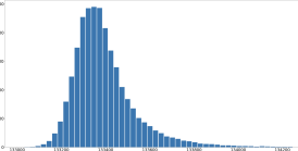
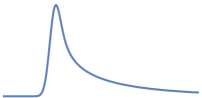
Figure 2. On the left, we obtain $G$ as a disjoint union of two independent Erdős–Rényi random graphs $\mathbb{G}(800,0.96)$, and we consider 500000 independent samples of a uniformly random vertex subsets $U$ with exactly 800 vertices. The resulting histogram for $e(G[U])$ may look approximately Gaussian, but closer inspection reveals asymmetry in the tails. This is not just an artifact of small numbers: the limiting distribution comes from a nontrivial quadratic polynomial of Gaussian random variables. Actually, it is possible for the skew to be much more exaggerated (the curve on the right shows one possibility for the limiting probability mass function of $e(G[U])$), but this is difficult to observe computationally, as this shape only really becomes visible for enormous graphs $G$.

In general, one can use a Gaussian invariance principle to show that the asymptotic conditional distribution of $e(G[U])$ always corresponds to some quadratic polynomial of Gaussian random variables; instead of proving a local central limit theorem, we need to prove some type of local limit theorem for convergence to that distribution.

In order to prove a local limit theorem of this type, it is necessary to ensure that the limiting distribution (some quadratic polynomial of Gaussian random variables) is “well-behaved”. This is where the tools discussed in Sections 1.2.2 and 1.2.3 come in: we prove that adjacency matrices of Ramsey graphs robustly have high rank, then apply certain variations of Theorem 1.6.

3.4. Controlling the characteristic function

We are now left with the task of actually proving the necessary local limit theorems. For this, we work in Fourier space, studying the characteristic functions $\varphi_{Y}\colon\tau\mapsto\mathbb{E}e^{i\tau Y}$ of certain random variables $Y$ (namely, we need to consider both the random variable $X=e(G[U])+\sum_{v\in U}e_{v}+e_{0}$ and certain conditional random variables arising in the additively structured case). Our aim is to compare $Y$ to an approximating random variable $Z$ (where $Z$ is either a Gaussian random variable or some quadratic polynomial of Gaussian random variables). This amounts to proving a suitable upper bound on $|\varphi_{Y}(\tau)-\varphi_{Z}(\tau)|$, for as broad a range of $\tau$ as possible (if one wants to precisely estimate point probabilities $\Pr[Y=x]$, it turns out that one needs to handle all $\tau$ in the range $[-\pi,\pi]$). We use different techniques for different ranges of $\tau\in\mathbb{R}$.

In the regime where $\tau$ is very small (e.g., when $|\tau|\leq n^{0.01}/\sigma(Y)$), $\varphi_{Y}(\tau)$ controls the large-scale distribution of $Y$, so depending on the setting we either employ standard techniques for proving central limit theorems, or a Gaussian invariance principle.

For larger $\tau$, it will be easy to show that our approximating characteristic function $\varphi_{Z}(\tau)$ is exponentially small in absolute value, so estimating $|\varphi_{Y}(\tau)-\varphi_{Z}(\tau)|$ amounts to proving an upper bound on $|\varphi_{Y}(\tau)|$, exploiting cancellation in $\mathbb{E}e^{i\tau Y}$ as $e^{i\tau Y}$ varies around the unit circle. Depending on the value of $\tau$, we are able to exploit cancellation from either the “linear” or the “quadratic” part of $Y$.

To exploit cancellation from the linear part, we adapt a decorrelation technique first introduced by Berkowitz [12] to study clique counts in random graphs (see also [85]), involving a subsampling argument and a Taylor expansion. While all previous applications of this technique exploited the particular symmetries and combinatorial structure of a specific polynomial of interest, here we instead take advantage of the robustness inherent in the definition of RLCD. We hope that these types of ideas will be applicable to the study of even more general types of polynomials.

To exploit cancellation from the quadratic part, we use the method of decoupling, building on arguments of the first and third authors [62]. Our improvements involve taking advantage of Fourier cancellation “on multiple scales”, which requires a sharpening of arguments of the first author and Sudakov [64] (building on work of Bukh and Sudakov [14]) concerning “richness” of Ramsey graphs.

The relevant ideas for all the Fourier-analytic estimates discussed in this subsection will be discussed in more detail in the appropriate sections of the paper (Sections 7 and 8).

3.5. Pointwise control via switching

Unfortunately, it seems to be extremely difficult to study the cancellations in $\varphi_{X}(\tau)$ for very large $\tau$, and we are only able to control the range where $|\tau|\leq\nu$ for some small constant $\nu=\nu(C)$ (recalling that $G$ is $C$-Ramsey). As a consequence, the above ideas only prove the following weakening of Theorem 2.1 (where we control the probability of $X$ lying in a constant-length interval instead of being equal to a particular value).

Theorem 3.1.

Fix $C>0$. There is $B=B(C)>0$ so the following holds for any fixed $H>0$. Let $G$ be an $C$-Ramsey graph with $n$ vertices, and consider $e_{0}\in\mathbb{R}$ and a vector $\vec{e}\in\mathbb{R}^{V(G)}$ with $0\leq e_{v}\leq Hn$ for all $v\in V(G)$. Let $U\subseteq V(G)$ be a random vertex subset obtained by including each vertex with probability $1/2$ independently, and let $X=e(G[U])+\sum_{v\in U}e_{v}+e_{0}$. Then

$$\sup_{x\in\mathbb{Z}}\Pr[|X-x|\leq B]\lesssim_{C,H}n^{-3/2},$$

and for every fixed $A>0$,

$$\inf_{\begin{subarray}{c}x\in\mathbb{Z}\\ |x-\mathbb{E}X|\leq An^{3/2}\end{subarray}}\Pr[|X-x|\leq B]\gtrsim_{C,H,A}n^{-3/2}.$$

Theorem 3.1 already implies the upper bound in Theorem 2.1, but not the lower bound. In Section 13, we deduce the desired lower bound on point probabilities from Theorem 3.1 (interestingly, this deduction requires both the lower and the upper bound in Theorem 3.1). As mentioned in the introduction, for this deduction, we introduce an “averaged” version of the so-called switching method. In particular, for $\ell\in\{-B,\ldots,B\}$, we consider the pairs of vertices $(y,z)$ with $y\in U$ and $z\notin U$ such that modifying $U$ by removing $y$ and adding $z$ (a “switch”) increases $e(G[U])$ by exactly $\ell$. We define random variables that measure the number of ways to perform such switches, and deduce Theorem 2.1 by studying certain moments of these random variables. Here we again need to use some arguments involving “richness” of Ramsey graphs, and we also make use of the technique of dependent random choice.

3.6. Technical issues

The above subsections describe the high-level ideas of the proof, but there are various technical issues that arise, some of which have a substantial impact on the complexity of the proof. Most importantly, in the additively structured case, we outlined how to prove a conditional local limit theorem for the quadratic part $Q$, but we completely swept under the rug how to then “integrate” this over outcomes of the conditioning. Explicitly, if we encode the bucket intersection sizes in a vector $\vec{\Delta}$, we have outlined how to use Fourier-analytic techniques to prove certain estimates on conditional probabilities of the form $\Pr[|X-x|\leq B|\vec{\Delta}]$, but we then need to average over the randomness of $\vec{\Delta}$ to obtain $\Pr\mathopen{}\mathclose{{}\left[|X-x|\leq B}\right]=\mathbb{E}[\Pr[|X-x|\leq B|\vec{\Delta}]]$ (taking into account that certain outcomes of $\vec{\Delta}$ give a much larger contribution than others).

There are certain relatively simple arguments with which we can accomplish this averaging while losing logarithmic factors in the final probability bound (namely, using a concentration inequality for $Q$ conditioned on $\vec{\Delta}$, we can restrict to only a certain range of outcomes $\vec{\Delta}$ which give a significant contribution to the overall probability $\Pr[|X-x|\leq B]$). To avoid logarithmic losses, we need to make sure that our conditional probability bounds “decay away from the mean”, which requires a non-uniform version of Theorem 1.6 (with a decay term), and some specialized tools for converting control of $|\varphi_{Y}(\tau)-\varphi_{Z}(\tau)|$ into bounds on small-ball probabilities for $Y$. Also, we need some delicate moment estimates comparing dependent random variables of “linear” and “quadratic” types, to quantify the dependence between certain fluctuations in the conditional mean and variance as we vary $\vec{\Delta}$.

Furthermore, for the switching argument described in the previous subsection, it is important (for technical reasons discussed in Remark 13.2) that in the setting of Theorem 3.1, $B$ does not depend on $A$ and $H$. To achieve this, we develop Fourier-analytic tools that take into account “local smoothness” properties of the approximating random variable $Z$.

3.7. Organization of the paper

In Section 4 we collect a variety of (mostly known) tools which will be used throughout the paper. Then, in Section 5 we prove Theorem 1.6 (our sharp small-ball probability estimate for quadratic polynomials of Gaussians), and in Section 6 we prove some general “relative” Esseen-type inequalities deducing bounds on small-ball probabilities from Fourier control.

In Sections 7 and 8 we obtain bounds on the characteristic function $\varphi_{X}(\tau)$ for various ranges of $\tau$ (specifically, bounds due to “cancellation of the linear part” appear in Section 7, and bounds due to “cancellation of the quadratic part” appear in Section 8). This is already enough to handle the additively unstructured case of Theorem 3.1, which we do in Section 9.

Most of the rest of the paper is then devoted to the additively structured case of Theorem 3.1. In Section 10 we study the “robust rank” of Ramsey graphs, and in Section 11 we prove some lemmas about quadratic polynomials on products of Boolean slices. All the ingredients collected so far come together in Section 12, where the additively structured case of Theorem 3.1 is proved.

Finally, in Section 13 we use a switching argument to deduce Theorem 2.1 from Theorem 3.1.

4. Preliminaries

In this section we collect some basic definitions and tools that will be used throughout the paper.

4.1. Basic facts about Ramsey graphs

First, as mentioned in the introduction, the following classical result about Ramsey graphs is due to Erdős and Szemerédi [36].

Theorem 4.1.

For any $C$, there exists $\varepsilon=\varepsilon(C)>0$ such that for every sufficiently large $n$, every $C$-Ramsey graph $G$ on $n$ vertices satisfies $\varepsilon\binom{n}{2}\leq e(G)\leq(1-\varepsilon)\binom{n}{2}$.

Remark 4.2.

In the setting of Remark 1.3, where $G$ has near-optimal spectral expansion, the expander mixing lemma (see for example [10, Corollary 9.2.5]) implies that (for sufficiently large $n$) all subsets of $G$ with at least $n^{1/2+0.02}$ vertices have density very close to the overall density of $G$. It is possible to use this fact in lieu of Theorem 4.1 in our proof of Theorem 2.1.

More recently, building on work of Bukh and Sudakov [14], the first author and Sudakov [64] proved that every Ramsey graph contains an induced subgraph in which the collection of vertex-neighborhoods is “rich”. Intuitively speaking, the richness condition here means that for all linear-size vertex subsets $W$, there are only very few vertex-neighborhoods that have an unusually large or unusually small intersection with $W$.

Definition 4.3.

Consider $\delta,\rho,\alpha>0$. We say that an $m$-vertex graph $G$ is $(\delta,\rho,\alpha)$-rich if for every subset $W\subseteq V(G)$ of size $|W|\geq\delta m$, there are at most $m^{\alpha}$ vertices $v\in V(G)$ with the property that $|N(v)\cap W|\leq\rho|W|$ or $|W\setminus N(v)|\leq\rho|W|$.

When the parameter $\alpha$ is omitted, it is assumed to take the value $1/5$. That is to say, we write “$(\delta,\rho)$-rich” to mean “$(\delta,\rho,1/5)$-rich”.

The following lemma is a slight generalization of [64, Lemma 4] (and is proved in the same way).

Lemma 4.4.

For any fixed $C,\alpha>0$, there exists $\rho=\rho(C,\alpha)$ with $0<\rho<1$ such that the following holds. For $n$ sufficiently large in terms of $C$ and $\alpha$, for any $m\in\mathbb{R}$ with $\sqrt{n}\leq m\leq\rho n$, and any $C$-Ramsey graph $G$ on $n$ vertices, there is an induced subgraph of $G$ on at least $m$ vertices which is $((m/n)^{\rho},\rho,\alpha)$-rich.

For two disjoint vertex sets $U,W$ in a graph $G$, we write $e(U,W)$ for the number of edges between $U,W$ and write $d(U,W)=e(U,W)/(|U||W|)$ for the density between $U,W$. We furthermore write $d(U)=e(U)/\binom{|U|}{2}$ for the density inside the set $U$.

Proof.

We introduce an additional parameter $K$, which will be chosen to be large in terms of $C$ and $\alpha$. We will then choose $\rho=\rho(C,\alpha)$ with $0<\rho<1$ to be small in terms of $K$, $C$, and $\alpha$. We do not specify the values of $K$ and $\rho$ ahead of time, but rather assume they are sufficiently large or small to satisfy certain inequalities that arise in the proof.

Let $\delta=(m/n)^{\rho}$ and suppose for the purpose of contradiction that every set of at least $m$ vertices fails to induce a $(\delta,\rho,\alpha)$-rich subgraph. We will inductively construct a sequence of induced subgraphs $G=G[U_{0}]\supseteq G[U_{1}]\supseteq\cdots\supseteq G[U_{K}]$ and disjoint vertex sets $S_{1},\ldots,S_{K}$ of size $|S_{1}|=\cdots=|S_{K}|=\lceil m^{\alpha}/2\rceil$ such that for each $i=1,\ldots,K$, we have $|U_{i}|\geq(\delta/4)|U_{i-1}|$ and $S_{i}\subseteq U_{i-1}\setminus U_{i}$, as well as

$$\big{[}e(S_{i},\{u\})\leq 4\rho\cdot|S_{i}|\text{ for all }u\in U_{i}\big{]}\text{ or }\big{[}e(S_{i},\{u\})\geq(1-4\rho)\cdot|S_{i}|\text{ for all }u\in U_{i}\big{]}.$$

This will suffice, as follows. First note that for each $i=1,\ldots,K$, we have

$$\big{[}d(S_{i},S_{j})\leq 4\rho\text{ for all }j\in\{i+1,\ldots,K\}\big{]}\text{ or }\big{[}d(S_{i},S_{j})\geq 1-4\rho\text{ for all }j\in\{i+1,\ldots,K\}\big{]}.$$

Without loss of generality suppose that the first case holds for at least half of the indices $i=1,\ldots,K$, and let $S$ be the union of the corresponding sets $S_{i}$. Then one can compute $d(S)\leq 4\rho+1/K$. On the other hand $|S|\geq(K/2)\cdot m^{\alpha}/2\geq m^{\alpha}\geq n^{\alpha/2}$ and therefore $G[S]$ is a $(2C/\alpha)$-Ramsey graph. However, now the density bound $d(S)\leq 4\rho+1/K$ contradicts Theorem 4.1 if $\rho$ is sufficiently small and $K$ is sufficiently large (in terms of $C$ and $\alpha$).

Let $U_{0}=V(G)$. For $i=1,\ldots,K$ we will construct the vertex sets $U_{i}$ and $S_{i}$, assuming that $U_{0},\ldots,U_{i-1}$ and $S_{1},\ldots,S_{i-1}$ have already been constructed. Note that we have $|U_{i-1}|\geq(\delta/4)^{i-1}n\geq(\delta/4)^{K}n=(m/n)^{\rho K}4^{-K}n\geq m$, using that $\rho K\leq 1/3$ and $m/n\leq\rho\leq 8^{-K}$ for $\rho$ being sufficiently small with respect to $K$. Therefore, by our assumption, $U_{i-1}$ must contain a set $W$ of at least $\delta|U_{i-1}|$ vertices and a set $Y$ of more than $|U_{i-1}|^{\alpha}\geq m^{\alpha}$ vertices contradicting $(\delta,\rho,\alpha)$-richness. Suppose without loss of generality that $|N(v)\cap W|\leq\rho|W|$ for at least half of the vertices $v\in Y$, and let $S_{i}\subseteq Y\subseteq U_{i-1}$ be a set of precisely $\lceil m^{\alpha}/2\rceil$ such vertices $v\in Y$. Then, let $U=W\setminus S_{i}\subseteq U_{i-1}\setminus S_{i}$ and note that we have $|U|\geq|W|/2$ since $|W|\geq\delta|U_{i-1}|\geq 4\cdot(\delta/4)^{K}n\geq 4m\geq 2|S_{i}|$. Furthermore, let $U_{i}\subseteq U$ be the set of vertices $u\in U$ with $e(S_{i},\{u\})\leq 4\rho\cdot|S_{i}|$. Now, we just need to show $|U_{i}|\geq(\delta/4)|U_{i-1}|$. To this end, note that for all $v\in S_{i}$ we have $e(\{v\},U)=|N(v)\cap U|\leq|N(v)\cap W|\leq\rho|W|\leq 2\rho|U|$. Hence,

$$|U\setminus U_{i}|\cdot 4\rho\cdot|S_{i}|\leq\sum_{w\in U\setminus U_{i}}e(S_{i},\{w\})=e(S_{i},U\setminus U_{i})\leq e(S_{i},U)=\sum_{v\in S_{i}}e(\{v\},U)\leq|S_{i}|\cdot 2\rho|U|,$$

implying that $|U\setminus U_{i}|\leq|U|/2$ and hence $|U_{i}|\geq|U|/2\geq|W|/4\geq(\delta/4)|U_{i-1}|$, as desired. ∎

Remark 4.5.

In the setting of Remark 1.3, where $G$ is dense and has near-optimal spectral expansion (and $n$ is sufficiently large), the expander mixing lemma can be used to prove that every induced subgraph of $G$ on at least $n^{0.9}$ vertices is $(n^{-0.05},0.005,\alpha)$-rich (and therefore Lemma 4.4 holds) for $\alpha\geq 0.2$. It is possible to use this in lieu of Lemma 4.4 in our proof of Theorem 2.1.

4.2. Characteristic functions and anticoncentration

For a real random variable $X$, recall that the characteristic function $\varphi_{X}\colon\mathbb{R}\to\mathbb{C}$ is defined by $\varphi_{X}(t)=\mathbb{E}[e^{itX}]$. Note that we have $|\varphi_{X}(t)|\leq 1$ for all $t\in\mathbb{R}$. If $\varphi_{X}(t)$ is absolutely integrable, then $X$ has a continuous density $p_{X}$, which can be obtained by the inversion formula

$$p_{X}(u)=\frac{1}{2\pi}\int_{-\infty}^{\infty}e^{-itu}\varphi_{X}(t)\,dt.$$ (4.1)

Next, recall the Lévy concentration function, which measures the maximum small ball probability.

Definition 4.6.

For a real random variable $X$ and $\varepsilon\geq 0$, we define $\mathcal{L}(X,\varepsilon)=\sup_{x\in\mathbb{R}}\Pr[|X-x|\leq\varepsilon]$.

If $X$ has a density $p_{X}$, then we trivially have $\mathcal{L}(X,\varepsilon)\leq\varepsilon\max_{x\in\mathbb{R}}p_{X}(x)$. We can also control small-ball probabilities using only a certain range of values of the characteristic function, via Esseen’s inequality (see for example [83, Lemma 6.4]):

Theorem 4.7.

There is $C_{\ref{thm:esseen}}>0$ so that for any real random variable $X$ and any $\varepsilon>0$, we have

$$\mathcal{L}(X,\varepsilon)\leq C_{\ref{thm:esseen}}\cdot\varepsilon\int_{-2/\varepsilon}^{2/\varepsilon}|\varphi_{X}(t)|\,dt.$$

In Section 6 we will prove some more sophisticated “relative” variants of Theorem 4.7.

4.3. Distance-to-integer estimates, and regularized least common denominator

For $r\in\mathbb{R}$, let $\|r\|_{\mathbb{R}/\mathbb{Z}}$ denote the (Euclidean) distance of $r$ to the nearest integer. Recall that the Rademacher distribution is the uniform distribution on the set $\{-1,1\}$. If $x$ is Rademacher-distributed, then for any $r\in\mathbb{R}$ we have the well-known estimate

$$|\mathbb{E}[\exp(irx)]|=|\!\cos(r)|\leq 1-\lVert r/\pi\rVert_{\mathbb{R}/\mathbb{Z}}^{2}\leq\exp(-\lVert r/\pi\rVert_{\mathbb{R}/\mathbb{Z}}^{2}).$$ (4.2)

If $\vec{\xi}\in\{0,1\}^{n}$ is a uniformly random length-$n$ binary vector, then for any $\vec{a}\in\mathbb{R}^{n}$ and any $b\in\mathbb{R}$, we can rewrite $\vec{a}\cdot\vec{\xi}+b$ as a weighted sum of independent Rademacher random variables. Specifically, we have $\vec{a}\cdot\vec{\xi}+b=\vec{r}\cdot\vec{x}+\mathbb{E}[\vec{a}\cdot\vec{\xi}+b]$, where $\vec{r}=\vec{a}/2\in\mathbb{R}^{n}$ and $\vec{x}\in\{-1,1\}^{n}$ is obtained from $\vec{\xi}\in\{0,1\}^{n}$ by replacing all zeroes by $-1$’s. Then $\vec{x}$ is uniformly random in $\{-1,1\}^{n}$, so 4.2 yields

$$|\mathbb{E}[\exp(i(\vec{a}\cdot\vec{\xi}+b))]|=|\mathbb{E}[\exp(i(\vec{r}\cdot\vec{x}))]|=\prod_{j=1}^{n}|\mathbb{E}[\exp(ir_{j}x_{j})]|\leq\exp\Bigg{(}-\sum_{j=1}^{n}\lVert a_{j}/(2\pi)\rVert_{\mathbb{R}/\mathbb{Z}}^{2}\Bigg{)}.$$ (4.3)

In the case where we want to study $\vec{a}\cdot\vec{x}$ where $\vec{x}\in\{0,1\}^{n}$ is a uniformly random binary vector with a given number of ones (i.e., a random vector on a Boolean slice), one has the following estimate.

Lemma 4.8.

Fix $c>0$. Let $\vec{a}\in\mathbb{R}^{n}$, and suppose that for some $0<\delta\leq 1/2$ there are disjoint pairs $\{i_{1},j_{1}\},\ldots,\{i_{M},j_{M}\}\subseteq[n]$ such that $\|(a_{i_{k}}-a_{j_{k}})/(2\pi)\|_{\mathbb{R}/\mathbb{Z}}\geq\delta$ for each $k=1,\ldots,M$. Let $s$ be an integer with $cn\leq s\leq(1-c)n$. Then for a random zero-one vector $\vec{\xi}\in\mathopen{}\mathclose{{}\left\{0,1}\right\}^{n}$ with exactly $s$ ones, we have

$$|\mathbb{E}[\exp(i(\vec{a}\cdot\vec{\xi}))]|\lesssim\exp\mathopen{}\mathclose{{}\left(-\Omega_{c}(M\delta^{2})}\right).$$

Lemma 4.8 can be deduced from [82, Theorem 1.1]. For the reader’s convenience we include an alternative proof, reducing it to 4.3.

Proof.

We may assume that $M\leq cn/4$ (indeed, noting that $M\leq n/2$ we can otherwise just replace $M$ by $\lfloor cn/4\rfloor$). The random vector $\vec{\xi}$ corresponds to a uniformly random subset $U\subseteq[n]$ of size $s$. Let us first expose the intersection sizes $|U\cap\{i_{1},j_{1}\}|,\ldots,|U\cap\{i_{M},j_{M}\}|$, one at a time. For each $k=1,\ldots,M$ we have $|U\cap\{i_{k},j_{k}\}|=1$ with probability at least $c(1-c)/4$ even when conditioning on any outcomes for the previously exposed intersection sizes $|U\cap\{i_{1},j_{1}\}|,\ldots,|U\cap\{i_{k-1},j_{k-1}\}|$. Hence the number of indices $k\in[M]$ with $|U\cap\{i_{k},j_{k}\}|=1$ stochastically dominates a binomial random variable with distribution $\mathrm{Bin}(M,c(1-c)/4)$. Thus, by a Chernoff bound (see e.g. Lemma 4.16), with probability at least $1-\exp(-\Omega_{c}(M))$ there is a set $K\subseteq[M]$ of at least $c(1-c)M/8$ indices $k$ with $|U\cap\{i_{k},j_{k}\}|=1$. Let us expose and condition on all coordinates of $\vec{\xi}\in\{0,1\}^{n}$ except those in $\bigcup_{k\in K}\{i_{k},j_{k}\}$. The only remaining randomness of the vector $\vec{\xi}\in\{0,1\}^{n}$ is that for each $k\in K$ we have either $\xi_{i_{k}}=1$ or $\xi_{j_{k}}=1$ (each with probability $1/2$, independently for all $k\in K$). Thus, after all of this conditioning, we have $\vec{a}\cdot\vec{\xi}=\sum_{k\in K}(a_{i_{k}}-a_{j_{k}})\xi_{i_{k}}+b$ for some $b\in\mathbb{R}$, where $(\xi_{i_{k}})_{k\in K}\in\{0,1\}^{K}$ is uniformly random. Thus, 4.3 implies $|\mathbb{E}[\exp(i(\vec{a}\cdot\vec{\xi}))]|\leq\exp(-\sum_{k\in K}\|(a_{i_{k}}-a_{j_{k}})/(2\pi)\|_{\mathbb{R}/\mathbb{Z}}^{2})\leq\exp(-\Omega_{c}(M\delta^{2}))$, as desired. ∎

The above estimates motivate the notion of the essential least common denominator (LCD) of a vector $\vec{v}\in\mathbb{S}^{n-1}\subseteq\mathbb{R}^{n}$ (where $\mathbb{S}^{n-1}$ is the unit sphere in $\mathbb{R}^{n}$). The following formulation of this notion was proposed by Rudelson (see [92, (1.17)] and the remarks preceding), in the context of random matrix theory.

Definition 4.9 (LCD).

For $t>0$, let $\log_{+}t=\max\{0,\log t\}$. For $L\geq 1$ and $\vec{v}\in\mathbb{S}^{n-1}\subseteq\mathbb{R}^{n}$, the (essential) least common denominator $D_{L}(\vec{v})$ is defined as

$$D_{L}(\vec{v})=\operatorname{inf}\mathopen{}\mathclose{{}\left\{\theta>0:\operatorname{dist}(\theta\vec{v},\mathbb{Z}^{n})<L\sqrt{\log_{+}(\theta/L)}}\right\}.$$

(Here $\operatorname{dist}(\theta\vec{v},\mathbb{Z}^{n})=\sqrt{\sum_{i=1}^{n}\|\theta v_{i}\|_{\mathbb{R}/\mathbb{Z}}^{2}}$ denotes the Euclidean distance from $\theta\vec{v}$ to the nearest point in the integer lattice $\mathbb{Z}^{n}$.)

The following lemma gives a lower bound on the LCD of a unit vector $\vec{v}$ in terms of $\lVert\vec{v}\rVert_{\infty}$.

Lemma 4.10 ([92, Lemma 6.2]).

If $\vec{v}\in\mathbb{S}^{n-1}$ and $L\geq 1$, then

$$D_{L}(\vec{v})\geq 1/(2\lVert\vec{v}\rVert_{\infty}).$$

Proof.

Note that for $\theta\leq 1/(2\lVert\vec{v}\rVert_{\infty})$ we have that $\lVert\theta\vec{v}\rVert_{\infty}\leq 1/2$. Thus we have that

$$\operatorname{dist}(\theta\vec{v},\mathbb{Z}^{n})=\operatorname{dist}(\theta\vec{v},\vec{0})=\theta>L\sqrt{\log_{+}(\theta/L)}$$

where we have used that $x>\sqrt{\log_{+}(x)}$ for $x>0$. The result follows by the definition of LCD. ∎

If $D_{L}(\vec{v})$ is large, then we can obtain strong control over the characteristic function of random variables of the form $\vec{v}\cdot\vec{x}$, for an i.i.d. Rademacher vector $\vec{x}$ (specifically, we are able to compare such characteristic functions to the characteristic function $\varphi_{Z}(t)=e^{-t^{2}/2}$ of a standard Gaussian $Z\sim\mathcal{N}(0,1)$). However, if $D_{L}(\vec{v})$ is small, then in a certain sense $\vec{v}$ is “additively structured”, and we can deduce certain combinatorial consequences. Actually, to obtain the consequences we need, we will use the following more robust notion known as regularized LCD, introduced by Vershynin [92].

Definition 4.11 (regularized LCD).

Fix $L\geq 1$ and $0<\gamma<1$. For a vector $\vec{v}\in\mathbb{R}^{n}$ with fewer than $n^{1-\gamma}$ zero coordinates, the regularized least common denominator (RLCD) $\widehat{D}_{L,\gamma}(\vec{v})$, is defined as

$$\widehat{D}_{L,\gamma}(\vec{v})=\max\{D_{L}(\vec{v}_{I}/\|\vec{v}_{I}\|_{2})\colon|I|=\lceil n^{1-\gamma}\rceil\},$$

where $\vec{v}_{I}\in\mathbb{R}^{I}$ denotes the restriction of $\vec{v}$ to the indices in $I$.

If a vector $\vec{d}$ is “additively structured” in the sense of having small RLCD, we can partition its index set into a small number of “buckets” such that the values of $d_{i}$ are similar inside each bucket. This is closely related to $\varepsilon$-net arguments using LCD assumptions that have previously appeared in the random matrix theory literature (see for example [83, Lemma 7.2]).

Lemma 4.12.

Fix $H>0$ and $0<\gamma<1/4$ and $L\geq 1$. Let $\vec{d}\in\mathbb{R}_{\geq 0}^{n}$ be a vector such that $\lVert\vec{d}\rVert_{\infty}\leq Hn$ and $\lVert\vec{d}_{S}\rVert_{2}\geq n^{3/2-2\gamma}$ for every subset $S\subseteq[n]$ of size $|S|=\lceil n^{1-\gamma}\rceil$, and assume that $n$ is sufficiently large with respect to $H$, $\gamma$ and $L$.

If $\widehat{D}_{L,\gamma}(\vec{d})\leq n^{1/2}$, then there exists a partition $[n]=R\cup(I_{1}\cup\cdots\cup I_{m})$ and real numbers $\kappa_{1},\ldots,\kappa_{m}\geq 0$ with $|R|\leq n^{1-\gamma}$ and $|I_{1}|=\cdots=|I_{m}|=\lceil n^{1-2\gamma}\rceil$ such that for all $j=1,\ldots,m$ and $i\in I_{j}$ we have $|d_{i}-\kappa_{j}|\leq n^{1/2+4\gamma}$.

Proof.

Choose a partition $[n]=R\cup(I_{1}\cup\cdots\cup I_{m})$ and $\kappa_{j}\geq 0$ for $j=1,\ldots,m$ with $|I_{1}|=\cdots=|I_{m}|=\lceil n^{1-2\gamma}\rceil$ such that $|d_{i}-\kappa_{j}|\leq n^{1/2+4\gamma}$ for all $1\leq j\leq m$ and $i\in I_{j}$, such that $m$ is as large as possible. It then suffices to prove that $|R|\leq n^{1-\gamma}$.

So let us assume for contradiction that $|R|>n^{1-\gamma}$, and fix a subset $S\subseteq R$ of size $|S|=\lceil n^{1-\gamma}\rceil$. Note that $D_{L}(\vec{d}_{S}/\lVert\vec{d}_{S}\rVert_{2})\leq\widehat{D}_{L,\gamma}(\vec{d})\leq n^{1/2}$ by Definition 4.11. Furthermore, since $\lVert\vec{d}_{S}/\lVert\vec{d}_{S}\rVert_{2}\rVert_{\infty}\leq Hn/n^{3/2-2\gamma}=Hn^{-1/2+2\gamma}$, Lemma 4.10 implies $D_{L}(\vec{d}_{S}/\lVert\vec{d}_{S}\rVert_{2})\geq H^{-1}n^{1/2-2\gamma}$. Thus, by Definition 4.9, there is some $\theta\in[H^{-1}n^{1/2-2\gamma},2n^{1/2}]$ such that

$$\lVert(\theta/\lVert\vec{d}_{S}\rVert_{2})\vec{d}_{S}-\vec{w}\rVert_{2}\leq L\sqrt{\log_{+}(\theta/L)}\leq L\sqrt{\log n}$$ (4.4)

for some $\vec{w}\in\mathbb{Z}^{S}$. By choosing $\vec{w}$ to minimize the left-hand side, we may assume that $\vec{w}$ has nonnegative entries (recall that $\vec{d}$ has nonnegative entries).

Now, the number of indices $i\in S$ with $|(\theta/\lVert\vec{d}_{S}\rVert_{2})d_{i}-w_{i}|>n^{-1/2+2\gamma}$ is at most

$$\frac{\lVert(\theta/\lVert\vec{d}_{S}\rVert_{2})\vec{d}_{S}-\vec{w}\rVert_{2}}{n^{-1+4\gamma}}\leq\frac{L\sqrt{\log n}}{n^{-1+4\gamma}}\leq n^{1-3\gamma}.$$

Furthermore, note that $\theta\leq 2n^{1/2}$ and 4.4 imply $\lVert\vec{w}\rVert_{2}\leq 3n^{1/2}$, and hence the number of indices $i\in S$ with $w_{i}\geq n^{2\gamma/3}$ is at most $9n^{1-4\gamma/3}$. Thus, as $|S|=\lceil n^{1-\gamma}\rceil$, there must be at least $|S|/2\geq n^{1-\gamma}/2$ indices $i\in S$ with $|(\theta/\lVert\vec{d}_{S}\rVert_{2})d_{i}-w_{i}|\leq n^{-1/2+2\gamma}$ and $w_{i}\in[0,n^{2\gamma/3}]\cap\mathbb{Z}$. Hence by the pigeonhole principle there is some $\kappa\geq 0$ and a subset $I_{m+1}\subseteq S\subseteq R$ of size $|I_{m+1}|=\lceil n^{1-2\gamma}\rceil$ such that for all $i\in I_{m+1}$ we have $w_{i}=\kappa$ and

$$|(\theta/\lVert\vec{d}_{S}\rVert_{2})d_{i}-\kappa|=|(\theta/\lVert\vec{d}_{S}\rVert_{2})d_{i}-w_{i}|\leq n^{-1/2+2\gamma}=\frac{n^{1/2-2\gamma}}{n^{(1-\gamma)/2}n}\cdot n^{1/2+(7/2)\gamma}\lesssim_{H}\frac{\theta}{\lVert\vec{d}_{S}\rVert_{2}}\cdot n^{1/2+(7/2)\gamma}.$$

Defining $\kappa_{m+1}=(\lVert\vec{d}_{S}\rVert_{2}/\theta)\kappa\geq 0$, this implies $|d_{i}-\kappa_{m+1}|\leq n^{1/2+4\gamma}$ for all $i\in I_{m+1}$. But now the partition $V(G)=(R\setminus I_{m+1})\cup(I_{1}\cup\cdots\cup I_{m+1})$ contradicts the maximality of $m$. ∎

4.4. Low-rank approximation

Recall the definition of the Frobenius norm (also called the Hilbert–Schmidt norm): for a matrix $M\in\mathbb{R}^{n\times n}$, we have

$$\|M\|_{\mathrm{F}}=\Big{(}\sum_{i,j=1}^{n}M_{ij}^{2}\Big{)}^{1/2}=\sqrt{\operatorname{trace}(M^{\intercal}M)}.$$

If $M$ is symmetric, then $\|M\|_{\mathrm{F}}^{2}$ is the sum of squares of the eigenvalues of $M$ (with multiplicity).

Famously, Eckart and Young [28] proved that for any real matrix $M$, the degree to which $M$ can be approximated by a low-rank matrix $\widetilde{M}$ can be described in terms of the spectrum of $M$. The following statement is specialized to the setting of real symmetric matrices.

Theorem 4.13.

Consider a symmetric matrix $M\in\mathbb{R}^{n\times n}$, and let $\lambda_{1},\ldots,\lambda_{n}$ be its eigenvalues. Then for any $r=0,\ldots,n$ we have

$$\min_{\begin{subarray}{c}\widetilde{M}\in\mathbb{R}^{n\times n}\\ \operatorname{rank}(\widetilde{M})\leq r\end{subarray}}\|M-\widetilde{M}\|^{2}_{\mathrm{F}}=\min_{\begin{subarray}{c}I\subseteq[n]\\ |I|=n-r\end{subarray}}\sum_{i\in I}\lambda_{i}^{2},$$

where the minimum is over all (not necessarily symmetric) matrices $\widetilde{M}\in\mathbb{R}^{n\times n}$ with rank at most $r$.

4.5. Analysis of Boolean functions

In this subsection we collect some tools from the theory of Boolean functions. A thorough introduction to the subject can be found in [78].

Consider a multilinear polynomial $f(x_{1},\ldots,x_{n})=\sum_{S\subseteq[n]}a_{S}\prod_{i\in S}x_{i}$. An easy computation shows that if $\vec{x}$ is a sequence of independent Rademacher or independent standard Gaussian random variables, then $\mathbb{E}[f(\vec{x})]=a_{\emptyset}$ and

$$\operatorname{Var}[f(\vec{x})]=\sum_{\emptyset\neq S\subseteq[n]}a_{S}^{2}.$$ (4.5)

Thus, in the case $\deg f=2$, we can consider the contributions to the variance $\operatorname{Var}[f(\vec{x})]$ coming from the “linear” part and the “quadratic” part. This will be important in our proof of Theorem 2.1.

We will need the following bound on moments of low-degree polynomials of Rademacher or standard Gaussian random variables (which is a special case of a phenomenon called hypercontractivity).

Theorem 4.14 ([78, Theorem 9.21]).

Let $f$ be a polynomial in $n$ variables of degree at most $d$. Let $\vec{x}=(x_{1},\ldots,x_{n})$ either be a vector of independent Rademacher random variables or a vector of independent standard Gaussian random variables. Then for any real number $q\geq 2$, we have

$$\mathbb{E}\big{[}|f(\vec{x})|^{q}\big{]}^{1/q}\leq\big{(}\sqrt{q-1}\big{)}^{d}\mathbb{E}\big{[}f(\vec{x})^{2}\big{]}^{1/2}.$$

We emphasize that we do not require $f(\vec{x})$ to have mean zero, so in the general setting of Theorem 4.14 one does not necessarily have $\mathbb{E}[f(\vec{x})^{2}]^{1/2}=\sigma(f(\vec{x}))$ (though in our proof of Theorem 2.1 we will only apply Theorem 4.14 in the case where $\mathbb{E}[f(\vec{x})]=0$).

Note that [78, Theorem 9.21] is stated only for Rademacher random variables; the Gaussian case of Theorem 4.14 follows by approximating Gaussian random variables with sums of Rademacher random variables, using the central limit theorem.

Next, one can use Theorem 4.14 to obtain the following concentration inequality. The Rademacher case is stated as [78, Theorem 9.23], and the Gaussian case may be proved in the same way.

Theorem 4.15.

Let $f$ be a polynomial in $n$ variables of degree at most $d$. Let $\vec{x}=(x_{1},\ldots,x_{n})$ either be a vector of independent Rademacher random variables or a vector of independent standard Gaussian random variables. Then for any $t\geq(2e)^{d/2}$,

$$\Pr\mathopen{}\mathclose{{}\left[|f(\vec{x})|\geq t(\mathbb{E}[f(x)^{2}])^{1/2}}\right]\leq\exp\mathopen{}\mathclose{{}\left(-\frac{d}{2e}t^{2/d}}\right).$$

4.6. Basic concentration inequalities

We will frequently need the Chernoff bound for binomial and hypergeometric distributions (see for example [56, Theorems 2.1 and 2.10]). Recall that the hypergeometric distribution $\mathrm{Hyp}(N,K,n)$ is the distribution of $|Z\cap U|$, for fixed sets $U\subseteq S$ with $|S|=N$ and $|U|=K$ and a uniformly random size-$n$ subset $Z\subseteq S$.

Lemma 4.16 (Chernoff bound).

Let $X$ be either:

• a sum of independent random variables, each of which take values in $\{0,1\}$, or

• hypergeometrically distributed (with any parameters).

Then for any $\delta>0$ we have

$$\Pr[X\leq(1-\delta)\mathbb{E}X]\leq\exp(-\delta^{2}\mathbb{E}X/2),\qquad\Pr[X\geq(1+\delta)\mathbb{E}X]\leq\exp(-\delta^{2}\mathbb{E}X/(2+\delta)).$$

We will also need the following concentration inequality, which is a simple consequence of the Azuma–Hoeffding martingale concentration inequality (a special case appears in [50, Corollary 2.2], and the general case follows from the same proof).

Lemma 4.17.

Consider a partition $[n]=I_{1}\cup\cdots\cup I_{m}$, and sequences $(\ell_{1},\ldots,\ell_{m}),(\ell_{1}^{\prime},\ldots,\ell_{m}^{\prime})\in\mathbb{N}^{m}$ with $\ell_{k}+\ell^{\prime}_{k}\leq|I_{k}|$ for $k=1,\ldots,m$ (and $\ell_{1}+\cdots+\ell_{m}+\ell_{1}^{\prime}+\cdots+\ell_{m}^{\prime}>0$). Let $S\subseteq\{-1,0,1\}^{n}$ be the set of vectors $\vec{x}\in\{-1,0,1\}^{n}$ such that $\vec{x}_{I_{k}}$ has exactly $\ell_{k}$ entries being $1$ and exactly $\ell_{k}^{\prime}$ entries being $-1$ for each $k=1,\ldots,m$. Let $a>0$ and suppose that $f\colon S\to\mathbb{R}$ is a function such that we have $|f(\vec{x})-f(\vec{x}^{\prime})|\leq a$ for any two vectors $\vec{x},\vec{x}^{\prime}\in S$ which differ in precisely two coordinates (i.e., which are obtained from each other by switching two entries inside some set $I_{k}$). Then for a uniformly random vector $\vec{x}\in S$ and any $t\geq 0$ we have

$$\Pr[|f(\vec{x})-\mathbb{E}f(\vec{x})|\geq t]\leq 2\exp\mathopen{}\mathclose{{}\left(-\frac{t^{2}}{2\cdot(\ell_{1}+\cdots+\ell_{m}+\ell_{1}^{\prime}+\cdots+\ell_{m}^{\prime})\cdot a^{2}}}\right).$$

Proof.

We sample a a uniformly random vector $\vec{x}\in S$ in $\ell:=\ell_{1}+\cdots+\ell_{m}+\ell_{1}^{\prime}+\cdots+\ell_{m}^{\prime}$ steps, as follows. In the first $\ell_{1}$ steps, we pick the $\ell_{1}$ indices $i\in I_{1}$ such that $x_{i}=1$ (at each step, pick an index $i\in I_{1}$ uniformly at random among the indices where $x_{i}$ is not yet defined, and define $x_{i}=1$). In the next $\ell_{2}$ steps we pick the $\ell_{2}$ indices $i\in I_{2}$ such that $x_{i}=1$, and so on. After $\ell_{1}+\cdots+\ell_{m}$ steps we have defined all the $1$-entries of $\vec{x}$. Now, we repeat the procedure (for $\ell_{1}^{\prime}+\cdots+\ell_{m}^{\prime}$ steps) for the $-1$-entries.

For $t=0,\ldots,\ell$, define $X_{t}$ to be the expectation of $f(\vec{x})$ conditioned on the coordinates of $\vec{x}$ defined up to step $t$. Then $X_{0},\ldots,X_{t}$ is the Doob martingale associated to our process of sampling $\vec{x}$. Note that $X_{0}=\mathbb{E}f(\vec{x})$ and $X_{\ell}=f(\vec{x})$.

We claim that we always have $|X_{t}-X_{t-1}|\leq a$ for $t=1,\ldots,\ell$. Indeed, let us condition on any outcomes of the first $t-1$ steps of our process of sampling $\vec{x}$. Now, for any two possible indices $i$ and $i^{\prime}$ chosen the $t$-th step, we can couple the possible outcomes of $\vec{x}$ if $i$ is chosen in the $t$-th step with the possible outcomes of $\vec{x}$ if $i^{\prime}$ is chosen in the $t$-th step, simply by switching the $i$-th and the $i^{\prime}$-th coordinate. Using our assumption on $f$, this shows that for any two possible outcomes in the $t$-th step the corresponding conditional expectations differ by at most $a$. This implies $|X_{t}-X_{t-1}|\leq a$, as claimed.

Now the inequality in the lemma follows from the Azuma–Hoeffding inequality for martingales (see for example [56, Theorem 2.25]). ∎

5. Small-ball probability for quadratic polynomials of Gaussians

In this section we prove Theorem 1.6, which we reproduce for the reader’s convenience. For the sake of convenience in the proofs and statements, in this section the notation $a\lesssim b$ simply means that $a\leq Cb$ for some constant $C$ (i.e., there is no stipulation that $n$, the number of variables, be large).

See 1.6

Remark 5.1.

By Theorem 4.13, the robust rank assumption in Theorem 1.6 is equivalent to the assumption that every subset $I\subseteq[n]$ of size $|I|=n-2$ satisfies $\sum_{i\in I}\lambda_{i}^{2}\geq\eta(\lambda_{1}^{2}+\cdots+\lambda_{n}^{2})$, where $\lambda_{1},\ldots,\lambda_{n}$ denote the eigenvalues of $F$.

We remark that for any real random variable $X$, one can use Chebyshev’s inequality to show that $\mathcal{L}(X,\varepsilon)=\Omega(\varepsilon/\sigma(X))$, so the bound in Theorem 1.6 is best-possible.

In the proof of Theorem 2.1, we will actually need a slightly more technical non-uniform version of Theorem 1.6 that decays away from the mean (at a high level, this is proved by combining Theorem 1.6 with the hypercontractive tail bound in Theorem 4.15, via a “splitting” technique). We will also need a lower bound on the probability that $f(\vec{Z})$ falls in a given interval of length $\varepsilon$, as long as this interval is relatively close to $\mathbb{E}f(\vec{Z})$, and lies on “the correct side” of $\mathbb{E}f(\vec{Z})$ (this lower bound requires no rank assumption).

Theorem 5.2.

Let $\vec{Z}=(Z_{1},\ldots,Z_{n})\sim\mathcal{N}(0,1)^{\otimes n}$ be a vector of independent standard Gaussian random variables. Consider a non-constant real quadratic polynomial $f(\vec{Z})$ of $\vec{Z}$, which we may write as

$$f(\vec{Z})=\vec{Z}^{\intercal}F\vec{Z}+\vec{f}\cdot\vec{Z}+f_{0}$$

for some symmetric matrix $F\in\mathbb{R}^{n\times n}$, some vector $\vec{f}\in\mathbb{R}^{n}$ and some $f_{0}\in\mathbb{R}$.

1. Suppose that $F$ is nonzero and

   $$\min_{\begin{subarray}{c}\widetilde{F}\in\mathbb{R}^{n\times n}\\ \operatorname{rank}(\widetilde{F})\leq 3\end{subarray}}\frac{\|F-\widetilde{F}\|^{2}_{\mathrm{F}}}{\|F\|^{2}_{\mathrm{F}}}\geq\eta.$$

   Then for any $x\in\mathbb{R}$ and any $0\leq\varepsilon\leq\sigma(f)$, we have

   $$\Pr[f-\mathbb{E}f\in[x,x+\varepsilon]]\lesssim_{\eta}\frac{\varepsilon}{\sigma(f)}\exp\mathopen{}\mathclose{{}\left(-\Omega\mathopen{}\mathclose{{}\left(\frac{|x|}{\sigma(f)}}\right)}\right).$$

2. Let $\lambda_{1},\ldots,\lambda_{n}$ be the eigenvalues of $F$. Suppose that $|\lambda_{i}|\leq\lambda_{1}$ for $i=1,\ldots,n$. Then for any $A>0$ and $0\leq\varepsilon\leq\sigma(f)$, we have

   $$\inf_{0\leq x\leq A\sigma(f)}\Pr[f-\mathbb{E}f\in[x,x+\varepsilon]]\gtrsim_{A}\frac{\varepsilon}{\sigma(f)}.$$

Remark 5.3.

Note that the infimum in (2) is only over nonnegative $x$. A two-sided bound is not possible in general, as the polynomial $f(\vec{Z})=Z_{1}^{2}$ shows. Also, while the rank assumption in Theorem 1.6 (robustly having rank at least 3) was best-possible, we believe that the rank assumption in Theorem 5.2(1) (robustly having rank at least 4) can be improved; it would be interesting to investigate this further (e.g., one might try to prove Theorem 5.2(1) directly rather than deducing it from Theorem 1.6).

In addition, in Theorem 5.2(2), the quantitative bound for implicit constant hidden by “$\gtrsim_{A}$” is rather poor; our proof provides a dependence of the form $\exp(-\exp(O(A^{2})))$. We believe that the correct dependence is $\exp(-O(A^{2}))$, and it may be interesting to prove this.

By orthogonal diagonalization of $F$ and the invariance of the distribution of $\vec{Z}$ under orthonormal transformations, in the proofs of Theorems 1.6 and 5.2 we can reduce to the case where $f(\vec{Z})=a_{0}+\sum_{i=1}^{n}(a_{i}Z_{i}+\lambda_{i}Z_{i}^{2})$ for some $a_{0},\ldots,a_{n}\in\mathbb{R}$. This is a sum of independent random variables, so we can proceed using Fourier-analytic techniques.

The rest of this section proceeds as follows. First, in Section 5.1, we prove Lemma 5.5, which encapsulates certain Fourier-analytic estimates that are effective when no individual term $a_{i}Z_{i}+\lambda_{i}Z_{i}^{2}$ contributes too much to the variance of $f(\vec{Z})$ (essentially, these are the estimates one needs for a central limit theorem).

Second, in Section 5.2 we prove the uniform upper bound in Theorem 1.6. In the case where no individual term contributes too much to the variance of $f(\vec{Z})$ we use Lemma 5.5, and otherwise we need some more specialized Fourier-analytic computations.

Third, in Section 5.3 we prove the lower bound in Theorem 5.2(2). Again, we use Lemma 5.5 in the case where no individual term contributes too much to the variance of $f(\vec{Z})$, while in the case where one of the terms is especially influential we perform an explicit (non-Fourier-analytic) computation.

Then, in Section 5.4 we deduce the non-uniform upper bound in Theorem 5.2(1) from Theorem 1.6, using a “splitting” technique.

Finally, in Section 5.5 we prove an auxiliary technical estimate on characteristic functions of quadratic polynomials of Gaussian random variables, in terms of the “rank robustness” of the quadratic polynomial (which we will need in the proof of Theorem 3.1).

5.1. Gaussian Fourier-analytic estimates

In this subsection we prove several Fourier-analytic estimates. First, we state a formula for the absolute value of the characteristic function of a univariate quadratic polynomial of a Gaussian random variable. One can prove this by direct computation, but we instead give a quick deduction from the formula for the characteristic function of a non-central chi-squared distribution (i.e., of a random variable $Z^{2}$ where $Z\sim\mathcal{N}(\mu,\sigma^{2})$; see for example [79]).

Lemma 5.4.

Let $W\sim\mathcal{N}(0,1)$ and let $X=aW+\lambda W^{2}$ for some $a,\lambda\in\mathbb{R}$. We have

$$|\varphi_{X}(t)|=\frac{\exp(-a^{2}t^{2}/(2+8\lambda^{2}t^{2}))}{(1+4\lambda^{2}t^{2})^{1/4}}.$$

Proof.

If $\lambda=0$, then $\varphi_{X}(t)=\varphi_{aW}(t)=\varphi_{W}(at)=\exp(-a^{2}t^{2}/2)$, as desired. So let us assume $\lambda\neq 0$. Note that $X=aW+\lambda W^{2}=\lambda(W+a/(2\lambda))^{2}-a^{2}/(4\lambda)$ and thus

$$|\varphi_{X}(t)|=|\varphi_{\lambda(W+a/(2\lambda))^{2}}(t)|=|\varphi_{(W+a/(2\lambda))^{2}}(\lambda t)|.$$

Using the formula for the characteristic function of a non-central chi-squared distribution with $1$ degree of freedom and non-centrality parameter $(a/(2\lambda))^{2}$, we obtain

$$|\varphi_{(W+a/(2\lambda))^{2}}(\lambda t)|=\frac{\mathopen{}\mathclose{{}\left|\exp\mathopen{}\mathclose{{}\left(\frac{i\cdot a^{2}/(4\lambda^{2})\cdot\lambda t}{1-2i\lambda t}}\right)}\right|}{|1-2i\lambda t|^{1/2}}=\frac{\mathopen{}\mathclose{{}\left|\exp\mathopen{}\mathclose{{}\left(\frac{i\cdot a^{2}/(4\lambda^{2})\cdot\lambda t\cdot(1+2i\lambda t)}{1+4\lambda^{2}t^{2}}}\right)}\right|}{(1+4\lambda^{2}t^{2})^{1/4}}=\frac{\exp\mathopen{}\mathclose{{}\left(\frac{-a^{2}t^{2}}{2(1+4\lambda^{2}t^{2})}}\right)}{(1+4\lambda^{2}t^{2})^{1/4}}.\qed$$

The crucial estimates in this subsection are encapuslated in the following lemma.

Lemma 5.5.

There are constants $C_{\ref{lem:gaussian-tricks}},C_{\ref{lem:gaussian-tricks}}^{\prime}>0$ such that the following holds. Let $W_{1},\ldots,W_{n}\sim\mathcal{N}(0,1)$ be independent standard Gaussian random variables, and fix sequences $\vec{a},\vec{\lambda}\in\mathbb{R}^{n}$ not both zero. Define random variables $X_{1},\ldots,X_{n}$ and $X$ as well as nonnegative $\sigma_{1},\ldots,\sigma_{n},\sigma,\Gamma\in\mathbb{R}$ by

$$X_{i}=a_{i}W_{i}+\lambda_{i}(W_{i}^{2}-1),\quad X=\sum_{i=1}^{n}X_{i},\quad\sigma_{i}^{2}=\sigma(X_{i})^{2}=a_{i}^{2}+2\lambda_{i}^{2},\quad\sigma^{2}=\sum_{i=1}^{n}\sigma_{i}^{2},\quad\Gamma=\frac{\sigma^{3}}{\sum_{i=1}^{n}\sigma_{i}^{3}}.$$

1. If $\int_{-\infty}^{\infty}\prod_{i=1}^{n}|\varphi_{X_{i}}(t)|\,dt<\infty$, then $X$ has a continuous density function $p_{X}\colon\mathbb{R}\to\mathbb{R}_{\geq 0}$ satisfying

   $$\sup_{u\in\mathbb{R}}\bigg{|}p_{X}(u)-\frac{e^{-u^{2}/(2\sigma^{2})}}{\sigma\sqrt{2\pi}}\bigg{|}\leq C_{\ref{lem:gaussian-tricks}}\bigg{(}\frac{1}{\Gamma\sigma}+\int_{|t|\geq\Gamma/(32\sigma)}\prod_{i=1}^{n}|\varphi_{X_{i}}(t)|\,dt\bigg{)}.$$

2. Furthermore if $\sigma_{i}^{2}\leq\sigma^{2}/4$ for all $i=1,\ldots,n$, then for any $K>0$, we have

   $$\int_{|t|\geq K/\sigma}\;\prod_{i=1}^{n}|\varphi_{X_{i}}(t)|\,dt\leq\frac{C_{\ref{lem:gaussian-tricks}}^{\prime}}{K\sigma}.$$

Remark 5.6.

Note that $\sigma^{3}=\sum_{i=1}^{n}\sigma_{i}^{2}\cdot\sigma\geq\sum_{i=1}^{n}\sigma_{i}^{3}$ and therefore $\Gamma\geq 1$.

The first part follows essentially immediately from the classical proof of the central limit theorem.

Proof of Lemma 5.5(a).

First, note that we may assume that there are no indices $i$ with $\sigma_{i}=0$ (indeed, if $\sigma_{i}=0$, then $\lambda_{i}=a_{i}=0$ and we can just omit all such indices). By rescaling, we may assume that $\sigma^{2}=1$. Note that $\varphi_{X}(t)=\prod_{i=1}^{n}\varphi_{X_{i}}(t)$, and hence $\int_{-\infty}^{\infty}|\varphi_{X}(t)|\,dt<\infty$. Also recall that the standard Gaussian distribution has density $u\mapsto e^{-u^{2}/2}/\sqrt{2\pi}$ and characteristic function $t\mapsto e^{-t^{2}/2}$. Thus, by the inversion formula 4.1, it suffices to show that

$$\frac{1}{2\pi}\int_{-\infty}^{\infty}\bigg{|}\prod_{i=1}^{n}\varphi_{X_{i}}(t)-e^{-t^{2}/2}\bigg{|}\,dt\lesssim\frac{1}{\Gamma}+\int_{|t|\geq\Gamma/32}\;\prod_{i=1}^{n}|\varphi_{X_{i}}(t)|\,dt.$$ (5.1)

Note that $\mathbb{E}[X_{i}]=0$ for $i=1,\ldots,n$, and let us write $L=(\sum_{i=1}^{n}\mathbb{E}[|X_{i}|^{3}])/(\sum_{i=1}^{n}\sigma_{i}^{2})^{3/2}=\sum_{i=1}^{n}\mathbb{E}[|X_{i}|^{3}]$. Then for $|t|\leq 1/(4L)$, by [80, Chapter V, Lemma 1] (which is a standard estimate in proofs of central limit theorems) we have

$$\bigg{|}\prod_{i=1}^{n}\varphi_{X_{i}}(t)-e^{-t^{2}/2}\bigg{|}=\mathopen{}\mathclose{{}\left|\varphi_{X}(t)-e^{-t^{2}/2}}\right|\leq 16L\cdot|t|^{3}e^{-t^{2}/3}.$$

By Hölder’s inequality and Theorem 4.14 (hypercontractivity) we have $\sigma_{i}^{3}\leq\mathbb{E}[|X_{i}|^{3}]\leq 8\sigma_{i}^{3}$ for $i=1,\ldots,n$, so we obtain $1/\Gamma\leq L\leq 8/\Gamma$. Thus, the interval $|t|\leq\Gamma/32$ contributes at most $\int_{-\Gamma/32}^{\Gamma/32}16L\cdot|t|^{3}e^{-t^{2}/3}\,dt\lesssim L\int_{-\infty}^{\infty}|t|^{3}e^{-t^{2}/3}\,dt\lesssim L\lesssim 1/\Gamma$ to the integral in 5.1. Therefore we obtain

$$\int_{|t|\geq{\Gamma}/{32}}\bigg{|}\prod_{i=1}^{n}\varphi_{X_{i}}(t)-e^{-t^{2}/2}\bigg{|}\,dt\leq\int_{|t|\geq{\Gamma}/{32}}e^{-t^{2}/2}+\bigg{|}\prod_{i=1}^{n}\varphi_{X_{i}}(t)\bigg{|}\,dt\lesssim\frac{1}{\Gamma}+\int_{|t|\geq{\Gamma}/{32}}\bigg{|}\prod_{i=1}^{n}\varphi_{X_{i}}(t)\bigg{|}\,dt.\qed$$

To prove Lemma 5.5(b), we use Hölder’s inequality and Lemma 5.4.

Proof of Lemma 5.5(b).

As before we may assume that there are no indices $i$ with $\sigma_{i}=0$, and by rescaling we may assume that $\sigma^{2}=1$. Via Lemma 5.4, we estimate

$$\int_{|t|\geq K}\bigg{|}\prod_{i=1}^{n}\varphi_{X_{i}}(t)\bigg{|}\,dt \leq\prod_{i=1}^{n}\bigg{(}\int_{|t|\geq K}|\varphi_{X_{i}}(t)|^{1/\sigma_{i}^{2}}\,dt\bigg{)}^{\sigma_{i}^{2}}=\prod_{i=1}^{n}\Bigg{(}\int_{|t|\geq K}\frac{\exp\Big{(}-{a_{i}^{2}t^{2}}/\mathopen{}\mathclose{{}\left({(2+8\lambda_{i}^{2}t^{2})\sigma_{i}^{2}}}\right)\Big{)}}{(1+4\lambda_{i}^{2}t^{2})^{1/(4\sigma_{i}^{2})}}\,dt\Bigg{)}^{\sigma_{i}^{2}}$$

$$\leq\prod_{i=1}^{n}\Bigg{(}\int_{|t|\geq K}\frac{\exp\Big{(}-{a_{i}^{2}t^{2}}/\mathopen{}\mathclose{{}\left({(2+8\lambda_{i}^{2}t^{2})\sigma_{i}^{2}}}\right)\Big{)}}{1+\lambda_{i}^{2}t^{2}/\sigma_{i}^{2}}\,dt\Bigg{)}^{\sigma_{i}^{2}}.$$

In the first step we have used Hölder’s inequality with weights $\sigma_{1}^{2},\ldots,\sigma_{n}^{2}$ (which sum to 1) and in the final step we have used Bernoulli’s inequality (which says that $(1+x)^{r}\geq 1+rx$ for $x\geq 0$ and $r\geq 1$; recall that we are assuming that $4(a_{i}^{2}+2\lambda_{i}^{2})=4\sigma_{i}^{2}\leq 1$ for each $i$).

Since $\sum_{i=1}^{n}\sigma_{i}^{2}=1$, it now suffices to prove that for each $i=1,\ldots,n$ we have

$$\int_{|t|\geq K}\frac{\exp\Big{(}-{a_{i}^{2}t^{2}}/\mathopen{}\mathclose{{}\left({(2+8\lambda_{i}^{2}t^{2})\sigma_{i}^{2}}}\right)\Big{)}}{1+\lambda_{i}^{2}t^{2}/\sigma_{i}^{2}}\,dt\lesssim\frac{1}{K}.$$

Fix some $i$. If $|\lambda_{i}|\geq|a_{i}|$, then $\lambda_{i}^{2}\geq\sigma_{i}^{2}/3$ and

$$\int_{|t|\geq K}\frac{\exp\Big{(}-{a_{i}^{2}t^{2}}/\mathopen{}\mathclose{{}\left({(2+8\lambda_{i}^{2}t^{2})\sigma_{i}^{2}}}\right)\Big{)}}{1+\lambda_{i}^{2}t^{2}/\sigma_{i}^{2}}\,dt\leq\int_{|t|\geq K}\frac{1}{1+t^{2}/3}\,dt\lesssim\frac{1}{K}.$$

Otherwise, if $|a_{i}|\geq|\lambda_{i}|$, we have $a_{i}^{2}\geq\sigma_{i}^{2}/3$, $\sigma_{i}^{2}\leq 1$, and therefore

$$\frac{\exp\Big{(}-{a_{i}^{2}t^{2}}/\mathopen{}\mathclose{{}\left({(2+8\lambda_{i}^{2}t^{2})\sigma_{i}^{2}}}\right)\Big{)}}{1+\lambda_{i}^{2}t^{2}/\sigma_{i}^{2}} \leq\frac{\Big{(}1+{a_{i}^{2}t^{2}}/\mathopen{}\mathclose{{}\left({(2+8\lambda_{i}^{2}t^{2})\sigma_{i}^{2}}}\right)\Big{)}^{-1}}{1+\lambda_{i}^{2}t^{2}/\sigma_{i}^{2}}$$

$$\lesssim\frac{\big{(}1+{t^{2}}/({1+\lambda_{i}^{2}t^{2}})\big{)}^{-1}}{1+\lambda_{i}^{2}t^{2}/\sigma_{i}^{2}}\leq\frac{\big{(}1+{t^{2}}/{(1+\lambda_{i}^{2}t^{2})}\big{)}^{-1}}{1+\lambda_{i}^{2}t^{2}}=\frac{1}{1+(1+\lambda_{i}^{2})t^{2}}.$$

It follows that

$$\int_{|t|\geq K}\frac{\exp\Big{(}-{a_{i}^{2}t^{2}}/\mathopen{}\mathclose{{}\left({(2+8\lambda_{i}^{2}t^{2})\sigma_{i}^{2}}}\right)\Big{)}}{1+\lambda_{i}^{2}t^{2}/\sigma_{i}^{2}}\,dt\lesssim\int_{|t|\geq K}\frac{1}{1+(1+\lambda_{i}^{2})t^{2}}\,dt\lesssim\frac{1}{K}.\qed$$

5.2. Uniform anticoncentration

In this section, we prove Theorem 1.6. The crucial ingredient is the following Fourier-analytic estimate.

Lemma 5.7.

Recall the definitions and notation in the statement of Lemma 5.5, and fix a parameter $\eta>0$. Suppose that $n\geq 2$ and $\sum_{i\in I}\lambda_{i}^{2}\geq\eta\lambda_{j}^{2}$ for all $I\subseteq[n]$ with $|I|=n-2$ and all $j\in[n]$. Then

$$\int_{|t|\geq 1/(32\sigma)}\prod_{i=1}^{n}|\varphi_{X_{i}}(t)|\,dt\lesssim_{\eta}\frac{1}{\sigma}.$$

Proof.

We may assume without loss of generality that $|\lambda_{1}|\geq\cdots\geq|\lambda_{n}|$. By adding at most two terms with $a_{i}=\lambda_{i}=0$, we may assume $n$ is divisible by $3$. Note that if $\sigma_{i}^{2}\leq\sigma^{2}/4$ for all $i\in[n]$, the result follows immediately from Lemma 5.5(b). Therefore it suffices to consider the case when there is an index $j$ such that $\sigma_{j}^{2}\geq\sigma^{2}/4$.

Note that the given condition implies $\sum_{k=1}^{n/3}\lambda_{3k}^{2}\geq\frac{1}{3}\sum_{k=3}^{n}\lambda_{k}^{2}\geq\eta\lambda_{j}^{2}/3$. Now, Lemma 5.4 yields

$$\prod_{i=1}^{n}|\varphi_{X_{i}}(t)| \leq\exp\bigg{(}\frac{-a_{j}^{2}t^{2}}{2+8\lambda_{j}^{2}t^{2}}\bigg{)}\prod_{i=1}^{n}\frac{1}{(1+4\lambda_{i}^{2}t^{2})^{1/4}}\leq\exp\bigg{(}\frac{-a_{j}^{2}t^{2}}{2+8\lambda_{j}^{2}t^{2}}\bigg{)}\prod_{i=1}^{n/3}\frac{1}{(1+4\lambda_{3i}^{2}t^{2})^{3/4}}$$

$$\leq\exp\bigg{(}\frac{-a_{j}^{2}t^{2}}{2+8\lambda_{j}^{2}t^{2}}\bigg{)}\bigg{(}1+4\sum_{i=1}^{n/3}\lambda_{3i}^{2}t^{2}\bigg{)}^{-3/4}\leq\exp\bigg{(}\frac{-a_{j}^{2}t^{2}}{2+8\lambda_{j}^{2}t^{2}}\bigg{)}(1+\eta\lambda_{j}^{2}t^{2})^{-3/4}$$

$$\leq\bigg{(}1+\frac{a_{j}^{2}t^{2}}{2+8\lambda_{j}^{2}t^{2}}\bigg{)}^{-3/4}(1+\eta\lambda_{j}^{2}t^{2})^{-3/4}\lesssim_{\eta}(\lambda_{j}^{2}t^{2}+a_{j}^{2}t^{2})^{-3/4}\lesssim(\sigma_{j}|t|)^{-3/2}\lesssim(\sigma|t|)^{-3/2}.$$

Thus we have

$$\int_{|t|\geq 1/(32\sigma)}\prod_{i=1}^{n}|\varphi_{X_{i}}(t)|\,dt\lesssim_{\eta}\int_{|t|\geq 1/(32\sigma)}(\sigma|t|)^{-3/2}\,dt\lesssim 1/\sigma.\qed$$

The proof of Theorem 1.6 is now immediate.

Proof of Theorem 1.6.

By rescaling we may assume $\sigma(f)=1$. It suffices to show that the probability density function $p_{f-\mathbb{E}f}$ of $f-\mathbb{E}f$ satisfies $p_{f-\mathbb{E}f}(u)\lesssim_{\eta}1$ for all $u$.

Since $F$ is a real symmetric matrix, we can write $F=QDQ^{\intercal}$ where $D$ is a diagonal matrix with entries $\lambda_{1},\ldots,\lambda_{n}$ and $Q$ is an orthogonal matrix. Let $\vec{W}=Q^{\intercal}\vec{Z}$, and note that $\vec{W}$ is also distributed as $\mathcal{N}(0,1)^{\otimes n}$ (since the distribution $\mathcal{N}(0,1)^{\otimes n}$ is invariant under orthogonal transformations). We have

$$f(\vec{Z})=f_{0}+\vec{f}\cdot\vec{Z}+\vec{Z}^{\intercal}F\vec{Z}=f_{0}+\vec{f}\cdot(Q\vec{W})+\vec{W}^{\intercal}Q^{\intercal}FQ\vec{W}=f_{0}+(Q^{\intercal}\vec{f})\cdot\vec{W}+\vec{W}^{\intercal}D\vec{W}.$$

Let $\vec{a}=(a_{1},\ldots,a_{n})=Q^{\intercal}\vec{f}$. We have

$$f-\mathbb{E}f=\sum_{i=1}^{n}(a_{i}W_{i}+\lambda_{i}(W_{i}^{2}-1)).$$

Let $\sigma_{1},\ldots,\sigma_{n}\geq 0$ be such that $\sigma_{i}^{2}=a_{i}^{2}+2\lambda_{i}^{2}$, so $1=\sigma(f)^{2}=\sigma_{1}^{2}+\cdots+\sigma_{n}^{2}$. Note that the assumption in the theorem statement implies $n\geq 3$, and combining the assumption with Theorem 4.13 yields

$$\eta\leq\min_{\begin{subarray}{c}\widetilde{F}\in\mathbb{R}^{n\times n}\\ \operatorname{rank}(\widetilde{F})\leq 2\end{subarray}}\frac{\|F-\widetilde{F}\|^{2}_{\mathrm{F}}}{\|F\|^{2}_{\mathrm{F}}}=\min_{\begin{subarray}{c}I\subseteq[n]\\ |I|=n-2\end{subarray}}\frac{\sum_{i\in I}\lambda_{i}^{2}}{\lambda_{1}^{2}+\cdots+\lambda_{n}^{2}}.$$

Hence for any subset $I\subseteq[n]$ with $|I|=n-2$ and any $j\in[n]$ we obtain $\sum_{i\in I}\lambda_{i}^{2}\geq\eta(\lambda_{1}^{2}+\cdots+\lambda_{n}^{2})\geq\eta\lambda_{j}^{2}$. Let $\Gamma$ be as in Lemma 5.5 and recall that $\Gamma\geq 1$.

Now, by combining Lemma 5.5(a) and Lemma 5.7, we have that

$$\sup_{u\in\mathbb{R}}p_{f}(u)=\sup_{u\in\mathbb{R}}p_{f-\mathbb{E}f}(u)\lesssim\frac{1}{\sqrt{2\pi}}+\frac{1}{\Gamma}+\int_{|t|\geq\Gamma/32}\prod_{i=1}^{n}|\varphi_{X_{i}}(t)|\,dt\lesssim_{\eta}1.$$

By integrating over the desired interval, we obtain the bound in Theorem 1.6. ∎

5.3. Lower bounds on small ball probabilities

Let us now prove the lower bound in Theorem 5.2(2). Note that Lemma 5.5(b) does not apply when some $\sigma_{i}$ is especially influential; in that case we will use the following bare-hands estimate.

Lemma 5.8.

Fix $A^{\prime}\geq 1$ and let $W\sim\mathcal{N}(0,1)$ and for some $a,\lambda\in\mathbb{R}$ (not both zero) let $X=aW+\lambda(W^{2}-1)$, so $\sigma(X)^{2}=a^{2}+2\lambda^{2}$. Suppose that

1. $\lambda\geq 0$, or

2. $\sigma(X)\geq 10A^{\prime}\cdot|\lambda|$.

Then for any $0\leq u\leq A^{\prime}\sigma(X)$, we have $p_{X}(u)\gtrsim_{A^{\prime}}1/{\sigma(X)}$.

Proof.

We may assume $a\geq 0$ (changing $a$ to $-a$ does not change the distribution of $X$). First note that the case $\lambda=0$ is easy, since then we have $\sigma(X)=a$ and $p_{X}(u)=e^{-(u/a)^{2}/2}/(\sqrt{2\pi}a)\gtrsim_{A^{\prime}}1/\sigma(X)$. So let us assume $\lambda\neq 0$ and define $g\colon\mathbb{R}\to\mathbb{R}$ by

$$g(t)=at+\lambda(t^{2}-1)=\lambda\cdot\mathopen{}\mathclose{{}\left(t+\frac{a}{2\lambda}}\right)^{2}-\lambda-\frac{a^{2}}{4\lambda}.$$

Then

$$(g^{\prime}(t))^{2}=4\lambda^{2}\cdot\mathopen{}\mathclose{{}\left(t+\frac{a}{2\lambda}}\right)^{2}=4\lambda\cdot g(t)+4\lambda^{2}+a^{2}\leq 4\sigma(X)\cdot|g(t)|+4\sigma(X)^{2}.$$

In particular, for any $t\in\mathbb{R}$ with $g(t)=u$, we obtain $|g^{\prime}(t)|\leq\sqrt{4(A^{\prime}+1)\sigma(X)^{2}}\lesssim_{A^{\prime}}\sigma(X)$.

We claim that we can find $t\in[-3A^{\prime},3A^{\prime}]$ with $g(t)=u$. Indeed, in case (1), we have $g(0)=-\lambda\leq u$ and $g(2A^{\prime}+1)\geq 2A^{\prime}a+2A^{\prime}\lambda\geq A^{\prime}\sigma(X)\geq u$, and hence by the intermediate value theorem there exists $t\in[0,2A^{\prime}+1]\subseteq[-3A^{\prime},3A^{\prime}]$ with $g(t)=u$. In case (2), observe that $a^{2}=\sigma(X)^{2}-2\lambda^{2}\geq 100A^{\prime 2}\cdot\lambda^{2}-2\lambda^{2}\geq 81A^{\prime 2}\cdot\lambda^{2}$, so $a\geq 9A^{\prime}\cdot|\lambda|$ and therefore $|\lambda(9A^{\prime 2}-1)|\leq A^{\prime}a$ and $\sigma(X)^{2}=a^{2}+2\lambda^{2}\leq 4a^{2}$. Hence $g(-3A^{\prime})=-3A^{\prime}a+\lambda(9A^{\prime 2}-1)\leq-2A^{\prime}a\leq 0\leq u$ and $g(3A^{\prime})=3A^{\prime}a+\lambda(9A^{\prime 2}-1)\geq 2A^{\prime}a\geq A^{\prime}\sigma(X)\geq u$ and we can again conclude that there exists $t\in[-3A^{\prime},3A^{\prime}]$ with $g(t)=u$.

Now, we have

$$p_{X}(u)=p_{g(W)}(g(t))\geq\frac{p_{W}(t)}{|g^{\prime}(t)|}\gtrsim_{A^{\prime}}\frac{e^{-(3A^{\prime})^{2}/2}}{\sigma(X)}\gtrsim_{A^{\prime}}\frac{1}{\sigma(X)}.\qed$$

We need one more ingredient for the proof of Theorem 5.2(2): a variant of the Paley-Zygmund inequality which tells us that under a fourth-moment condition, random variables are reasonably likely to have small fluctuations in a given direction. We include a short proof; the result can also easily be deduced from [5, Lemma 3.2(i)].

Lemma 5.9.

Fix $B\geq 1$. If $X$ is a real random variable with $\mathbb{E}[X]=0$ and $\sigma(X)>0$ satisfying $\mathbb{E}[X^{4}]\leq B\sigma(X)^{4}$, then

$$\Pr[-2\sqrt{B}\sigma(X)\leq X\leq 0]\geq 1/(5B).$$

Proof.

By rescaling we may assume that $\sigma(X)=1$. Note that then

$$9B^{2}\cdot\Pr[-2\sqrt{B}\leq X\leq 0] =\mathbb{E}[9B^{2}\mathbbm{1}_{-2\sqrt{B}\leq X\leq 0}]$$

$$\geq\mathbb{E}[-X(X+2\sqrt{B})(X-\sqrt{B})^{2}]$$

$$=-\mathbb{E}[X^{4}]+3B\cdot\mathbb{E}[X^{2}]-2B^{3/2}\mathbb{E}[X]=-\mathbb{E}[X^{4}]+3B\geq 2B$$

where we have used that $-x(x+2\sqrt{B})(x-\sqrt{B})^{2}=(B-(x+\sqrt{B})^{2})(x-\sqrt{B})^{2}\leq 9B^{2}\mathbbm{1}_{-2\sqrt{B}\leq x\leq 0}$ for all $x\in\mathbb{R}$. The result follows. ∎

Now we prove Theorem 5.2(2).

Proof of Theorem 5.2(2).

We may assume $\sigma(f)=1$. Borrowing the notation from the proof of Theorem 1.6, we write

$$f-\mathbb{E}f=\sum_{i=1}^{n}(a_{i}W_{i}+\lambda_{i}(W_{i}^{2}-1)),$$

with $(W_{1},\ldots,W_{n})\sim\mathcal{N}(0,1)^{\otimes n}$, and $\sigma_{i}^{2}=a_{i}^{2}+2\lambda_{i}^{2}$ (then we have $1=\sigma^{2}=\sigma_{1}^{2}+\cdots+\sigma_{n}^{2}$). It now suffices to prove that for all $u\in[0,A+1]$ we have $p_{f-\mathbb{E}f}(u)\gtrsim_{A}1$. Let $L$ be a large integer depending only on $A$ (such that $L\geq 2$ and $L\geq C_{\ref{lem:gaussian-tricks}}(1+32C_{\ref{lem:gaussian-tricks}}^{\prime})\cdot 2\sqrt{2\pi}\cdot e^{(A+1)^{2}/2}$ for the constants $C_{\ref{lem:gaussian-tricks}}$ and $C_{\ref{lem:gaussian-tricks}}^{\prime}$ in Lemma 5.5). We break into cases.

First, suppose $\max_{i}\sigma_{i}\leq 1/L$. In this case, we define $\Gamma=\sigma(f)^{3}/\sum_{i=1}^{n}\sigma_{i}^{3}=1/\sum_{i=1}^{n}\sigma_{i}^{3}$ and note that $\sum_{i=1}^{n}\sigma_{i}^{3}\leq(\max_{i}\sigma_{i})(\sum_{i=1}^{n}\sigma_{i}^{2})\leq 1/L$, so $\Gamma\geq L$. We also have $\sigma_{i}^{2}\leq 1/L^{2}\leq 1/4$, so Lemma 5.5(b) applies. So by combining parts (a) and (b) of Lemma 5.5, for all $u\in[0,A+1]$ we obtain, as desired,

$$p_{f-\mathbb{E}f}(u)\geq\frac{e^{-u^{2}/2}}{\sqrt{2\pi}}-\frac{C_{\ref{lem:gaussian-tricks}}(1+32C_{\ref{lem:gaussian-tricks}}^{\prime})}{\Gamma}\geq\frac{e^{-(A+1)^{2}/2}}{\sqrt{2\pi}}-\frac{C_{\ref{lem:gaussian-tricks}}(1+32C_{\ref{lem:gaussian-tricks}}^{\prime})}{L}\geq\frac{1}{2}\cdot\frac{e^{-(A+1)^{2}/2}}{\sqrt{2\pi}}\gtrsim_{A}1.$$

Otherwise, there is $i^{*}\in[n]$ such that $\sigma_{i^{*}}\geq 1/L$. We claim that then there is an index $j\in[n]$ satisfying at least one of the following two conditions:

• $\sigma_{j}\geq 1/(10(A+19)L^{2})$ and $\lambda_{j}\geq 0$, or

• $\sigma_{j}\geq 1/L$ and $10(A+19)L\cdot|\lambda_{j}|\leq\sigma_{j}$.

Indeed, if $10(A+19)L\cdot|\lambda_{i^{*}}|\leq\sigma_{i^{*}}$ we can simply take $j=i^{*}$ and (2) is satisfied. Otherwise we have $|\lambda_{i^{*}}|>\sigma_{i^{*}}/(10(A+19)L)\geq 1/(10(A+19)L^{2})$ and the assumption in Theorem 5.2(2) yields $\lambda_{1}\geq|\lambda_{i^{*}}|\geq 1/(10(A+19)L^{2})$. So in particular $\lambda_{1}\geq 0$ and $\sigma_{1}\geq\lambda_{1}\geq 1/(10(A+19)L^{2})$ and we can take $j=1$ and (1) is satisfied.

Now, let $X_{j}=a_{j}W_{j}+\lambda_{j}(W_{j}^{2}-1)$ and let $X^{\prime}=f-\mathbb{E}f-X_{j}=\sum_{i\neq j}(a_{i}W_{i}+\lambda_{i}(W_{i}^{2}-1))$ contain all terms of $f-\mathbb{E}f$ except the term $X_{j}$. By Theorem 4.14 (hypercontractivity) we have $\mathbb{E}[(X^{\prime})^{4}]\leq 81\sigma(X^{\prime})^{4}$ and therefore Lemma 5.9 shows that $-18\leq-18\sigma(X^{\prime})\leq X^{\prime}\leq 0$ with probability at least $1/405$.

We claim that we can apply Lemma 5.8 to $X_{j}$ and $u\in[0,A+19]$, showing that $p_{X_{j}}(u)\gtrsim_{A}1/\sigma_{j}\geq 1$. Indeed, in case (1) we have $0\leq u\leq 10(A+19)^{2}L^{2}\sigma_{j}$ and can apply case (1) of Lemma 5.8 with $A^{\prime}=10(A+19)^{2}L^{2}$, while in case (2) we have $0\leq u\leq(A+19)L\sigma_{j}$ and can apply case (2) of Lemma 5.8 with $A^{\prime}=(A+19)L$.

Therefore, for any $u\in[0,A+1]$ we obtain

$$p_{f-\mathbb{E}f}(u)=p_{X^{\prime}+X_{j}}(u)\geq\int_{-18}^{0}p_{X^{\prime}}(y)p_{X_{j}}(u-y)\,dy\gtrsim_{A}\int_{-18}^{0}p_{X^{\prime}}(y)\,dy=\Pr[-18\leq X^{\prime}\leq 0]\gtrsim 1.\qed$$

5.4. Non-uniform anticoncentration

In this subsection we prove Theorem 5.2(1), which is essentially a non-uniform version of Theorem 1.6. We begin with a lemma giving non-uniform anticoncentration bounds for a quadratic polynomial of a single Gaussian variable, i.e., for one of the terms in our sum.

Lemma 5.10.

Let $W\sim\mathcal{N}(0,1)$ and for some $a,\lambda\in\mathbb{R}$ (not both zero) let $X=aW+\lambda(W^{2}-1)$, so $\sigma:=\sigma(X)=a^{2}+2\lambda^{2}$. Then for $x\geq 10^{3}\sigma$ the following statements hold.

1. If $|\lambda|\cdot x>a^{2}/10$, then

   $$\Pr[|X|\geq x/6]\lesssim\frac{|\lambda|}{\sigma}\exp\mathopen{}\mathclose{{}\left(-\frac{x}{10^{3}\sigma}}\right)$$

2. If $|\lambda|\cdot x\leq a^{2}/10$, then for each $u\in\mathbb{R}$ with $x/10\leq|u|\leq 2x$, we have

   $$p_{X}(u)\lesssim\frac{1}{|a|}\exp\mathopen{}\mathclose{{}\left(-\frac{x}{\sigma}}\right)$$

Proof.

First consider part (1), and note that the assumption there implies that $\lambda\neq 0$. We claim that whenever $|X|\geq x/6$ holds, we must have $|W|>\sqrt{x/|\lambda|}/20$. Indeed, if $|W|\leq\sqrt{x/|\lambda|}/20$, then (using that $x\geq 10^{3}\sigma\geq 10^{3}|\lambda|$ and $a^{2}\leq 10|\lambda|\cdot x$)

$$|X|=|aW+\lambda(W^{2}-1)|\leq|a|\cdot\frac{\sqrt{x/|\lambda|}}{20}+|\lambda|\cdot\max\mathopen{}\mathclose{{}\left\{\frac{x/|\lambda|}{400},1}\right\}\leq\sqrt{10|\lambda|x}\cdot\frac{\sqrt{x/|\lambda|}}{20}+|\lambda|\cdot\frac{x/|\lambda|}{400}<\frac{x}{6}.$$

Thus, we obtain

$$\Pr\mathopen{}\mathclose{{}\left[|X|\geq\frac{x}{6}}\right]\leq\Pr\mathopen{}\mathclose{{}\left[|W|\geq\frac{\sqrt{x/|\lambda|}}{20}}\right]\lesssim\exp\mathopen{}\mathclose{{}\left(-\frac{x}{10^{3}|\lambda|}}\right) =\exp\mathopen{}\mathclose{{}\left(-\frac{x}{10^{3}\sigma}}\right)\cdot\exp\mathopen{}\mathclose{{}\left(-\frac{x}{10^{3}\sigma}\mathopen{}\mathclose{{}\left(\frac{\sigma}{|\lambda|}-1}\right)}\right)$$

$$\lesssim\exp\mathopen{}\mathclose{{}\left(-\frac{x}{10^{3}\sigma}}\right)\cdot\exp\mathopen{}\mathclose{{}\left(-\frac{\sigma}{|\lambda|}}\right)\lesssim\frac{|\lambda|}{\sigma}\exp\mathopen{}\mathclose{{}\left(-\frac{x}{10^{3}\sigma}}\right),$$

where in the second-last step we used that $x\geq 10^{3}\sigma$ and in the last step we used that the function $t\mapsto te^{-t}$ is bounded on $\mathbb{R}$.

For part (2), define the function $g\colon\mathbb{R}\to\mathbb{R}$ by $g(t)=at+\lambda(t^{2}-1)$. As in the proof of Lemma 5.8, we can calculate $(g^{\prime}(t))^{2}=4\lambda\cdot g(t)+4\lambda^{2}+a^{2}$ for all $t\in\mathbb{R}$. Now, consider some $u\in\mathbb{R}$ with $x/10\leq|u|\leq 2x$. There are at most two different $t\in\mathbb{R}$ with $g(t)=u$. For any such $t$, we have (using the assumption that $|\lambda|\cdot x\leq a^{2}/10$)

$$(g^{\prime}(t))^{2}\geq 4\lambda^{2}+a^{2}-4|\lambda|\cdot 2x\geq a^{2}/5\geq a^{2}/9.$$

We furthermore claim that any such $t$ must satisfy $|t|\geq x/(20|a|)$. Indeed, if $|t|<x/(20|a|)$, then (using that $x\geq 10^{3}\sigma\geq 10^{3}a$ and the assumption $|\lambda|\cdot x\leq a^{2}/10$)

$$|g(t)|=|at+\lambda(t^{2}-1)|\leq|a|\cdot\frac{x}{20|a|}+|\lambda|\cdot\max\mathopen{}\mathclose{{}\left\{\frac{x^{2}}{400a^{2}},1}\right\}\leq\frac{x}{20}+|\lambda|\cdot\frac{x^{2}}{400a^{2}}\leq\frac{x}{20}+\frac{x}{4000}<\frac{x}{10}.$$

As $|u|\geq x/10$, this contradicts $g(t)=u$. Thus any $t\in\mathbb{R}$ with $g(t)=u$ must indeed also satisfy $|t|\geq x/(20|a|)$. Now, we obtain (using again that $x\geq 10^{3}\sigma\geq 10^{3}a$)

$$p_{X}(u)=\sum_{\begin{subarray}{c}t\in\mathbb{R}\\ g(t)=u\end{subarray}}\frac{p_{W}(t)}{|g^{\prime}(t)|}\leq 2\cdot\frac{1}{|a|/3}\cdot\exp\mathopen{}\mathclose{{}\left(-\frac{x^{2}}{800a^{2}}}\right)\lesssim\frac{1}{|a|}\exp\mathopen{}\mathclose{{}\left(-\frac{x}{\sigma}}\right).\qed$$

Now, we prove Theorem 5.2(1). The main idea is to divide our random variable $f-\mathbb{E}f$ into independent parts, to take advantage of exponential tail bounds (by Theorem 4.15 or Lemma 5.10) for one of the parts, and anticoncentration bounds (by Theorem 1.6) for the rest of the parts.

Proof of Theorem 5.2(1).

By rescaling, we may assume $\sigma:=\sigma(f)=1$. If $|x|\leq 10^{3}=10^{3}\sigma(f)$, the desired bound follows from Theorem 1.6. So we may assume that $|x|\geq 10^{3}\sigma(f)$. Borrowing the notation from the proof of Theorem 1.6, we write

$$f-\mathbb{E}f=\sum_{i=1}^{n}(a_{i}W_{i}+\lambda_{i}(W_{i}^{2}-1)),$$

with $(W_{1},\ldots,W_{n})\sim\mathcal{N}(0,1)^{\otimes n}$ and $\sigma_{i}^{2}=a_{i}^{2}+2\lambda_{i}^{2}$ (then we have $1=\sigma^{2}=\sigma_{1}^{2}+\cdots+\sigma_{n}^{2}$). We may assume that $|\lambda_{1}|\geq\cdots\geq|\lambda_{n}|$. Note that using Theorem 4.13 the assumption in Theorem 5.2(1) implies that for every subset $I\subseteq[n]$ of size $|I|=n-3$ we have $\sum_{i\in I}\lambda_{i}^{2}\geq\eta(\lambda_{1}^{2}+\cdots+\lambda_{n}^{2})$. In particular, $\sum_{i=4}^{n}\lambda_{i}^{2}\geq\eta(\lambda_{1}^{2}+\cdots+\lambda_{n}^{2})$.

By adding at most three terms with $a_{i}=\lambda_{i}=0$, we may assume that $n\equiv 1\pmod{4}$. For a subset $J\subseteq[n]$, let $X_{J}=\sum_{i\in J}(a_{i}W_{i}+\lambda_{i}(W_{i}^{2}-1))$ and $\sigma_{J}^{2}=\sum_{i\in J}\sigma_{i}^{2}=\sigma(X_{J})^{2}$.

Let $i^{*}\in[n]$ be chosen such that $\sigma_{i^{*}}^{2}$ is maximal, and define $J_{0}=\{i^{*}\}$. We claim that we can find a partition of $[n]\setminus J_{0}=[n]\setminus\{i^{*}\}$ into four subsets $J_{1},J_{2},J_{3},J_{4}$ satisfying the following conditions.

1. For $h=1,2,3,4$, we have $\sigma_{[n]\setminus J_{h}}^{2}\geq\eta/2$.

2. For any $h=0,\ldots,4$ and any subset $I\subseteq[n]\setminus J_{h}$ of size $|I|=n-|J_{h}|-2$, we have $\sum_{i\in I}\lambda_{i}^{2}\geq(\eta/4)\cdot(\lambda_{1}^{2}+\cdots+\lambda_{n}^{2})$.

Indeed, we can build such a partition iteratively: let us divide $[n]\setminus\{i^{*}\}$ into $n/4$ quadruplets (starting with the four smallest indices, then the next four, and so on). Iteratively, for each quadruplet, distribute one element to each of $J_{1},J_{2},J_{3},J_{4}$ in the following way. We assign the index $i$ in the quadruplet with the largest $\sigma_{i}^{2}$ to the set $J_{h}$ which had the smallest value of $\sigma_{J_{h}}^{2}$ at the end of the last step, we assign the index $i$ with the second-largest $\sigma_{i}^{2}$ to the set $J_{h}$ which had the second-smallest value of $\sigma_{J_{h}}^{2}$, and so on. One can check that this assignment process maintains the property that at the end of any step, the value $\sigma_{J_{h}}^{2}$ for $h=1,2,3,4$ differ by at most $\max_{i}\sigma_{i}^{2}=\sigma_{i^{*}}^{2}$. Hence $\sigma_{[n]\setminus J_{1}}^{2}\geq\sigma_{J_{2}}^{2}+\sigma_{i^{*}}^{2}\geq\sigma_{J_{1}}^{2}=1-\sigma_{[n]\setminus J_{1}}^{2}$, so $\sigma_{[n]\setminus J_{1}}^{2}\geq 1/2\geq\eta/2$. Analogously, one can show $\sigma_{[n]\setminus J_{h}}^{2}\geq\eta/2$ for $h=2,3,4$, so (a) is satisfied. To check (b), note that for each $h=0,\ldots,4$ the set $[n]\setminus J_{h}$ is missing either one element from each of the quadruplets considered during the construction (if $1\leq h\leq h$) or is missing one element in total (if $h=0$). For a subset $I\subseteq[n]\setminus J_{h}$ of size $|I|=n-|J_{h}|-2$, two additional elements are missing. Thus, for every $k=1,\ldots,n/4$ the set $I\subseteq[n]$ is missing at most $k+2$ of the elements in $[4k]$. Thus, recalling that $|\lambda_{1}|\geq\cdots\geq|\lambda_{n}|$, we obtain

$$\sum_{i\in I}\lambda_{i}^{2}\geq\lambda_{4}^{2}+(\lambda_{6}^{2}+\lambda_{7}^{2}+\lambda_{8}^{2})+(\lambda_{10}^{2}+\lambda_{11}^{2}+\lambda_{12}^{2})+\cdots\geq\lambda_{4}^{2}+\lambda_{8}^{2}+\lambda_{12}^{2}+\cdots\geq\frac{1}{4}\sum_{i=4}^{n}\lambda_{i}^{2}\geq(\eta/4)\cdot(\lambda_{1}^{2}+\cdots+\lambda_{n}^{2}).$$

This establishes (b). Thus, the sets $J_{1},\ldots,J_{4}$ indeed satisfy the desired conditions.

By our assumption $|x|\geq 10^{3}\sigma(f)$ and by $0\leq\varepsilon\leq\sigma(f)$, we have $|y|\geq 0.999|x|\geq(5/6)\cdot|x|$ for all $y\in[x,x+\varepsilon]$. Thus, whenever $f-\mathbb{E}f=\sum_{i=1}^{n}(a_{i}W_{i}+\lambda_{i}(W_{i}^{2}-1))=X_{J_{0}}+\cdots+X_{J_{4}}$ is contained in the interval $[x,x+\varepsilon]$, we must have $|X_{J_{h}}|\geq|x|/6$ for at least one $h\in\{0,\ldots,4\}$.

We now distinguish several cases. First, consider the case that $\sigma_{i^{*}}^{2}\leq 1-(\eta/2)$. Then (recalling that $J_{0}=\{i^{*}\}$), we have $\sigma_{[n]\setminus J_{0}}^{2}=1-\sigma_{i^{*}}^{2}\geq\eta/2$, so condition (a) is also satisfied for $h=0$. We now have

$$\Pr[f-\mathbb{E}f\in[x,x+\varepsilon]] \leq\sum_{h=0}^{4}\Pr\Big{[}|X_{J_{h}}|\geq|x|/6\text{ and }X_{[n]\setminus J_{h}}\in[x-X_{J_{h}},x-X_{J_{h}}+\varepsilon]\Big{]}$$

$$\leq\sum_{h=0}^{4}\Pr[|X_{J_{h}}|\geq|x|/6]\cdot\mathcal{L}(X_{[n]\setminus J_{h}},\varepsilon)$$

$$\lesssim_{\eta}\sum_{h=0}^{4}\exp\mathopen{}\mathclose{{}\left(-\frac{2}{2e}\cdot\frac{|x|}{6\sigma_{J_{h}}}}\right)\cdot\frac{\varepsilon}{\sigma_{[n]\setminus J_{h}}}\lesssim_{\eta}\frac{\varepsilon}{\sigma}\exp\mathopen{}\mathclose{{}\left(-\Omega\mathopen{}\mathclose{{}\left(\frac{|x|}{\sigma}}\right)}\right),$$

where in the third step we applied Theorem 4.15 to $X_{J_{h}}$ with $t=|x|/(6\sigma_{J_{h}})\geq|x|/(6\sigma)$ and Theorem 1.6 to $X_{[n]\setminus J_{h}}$ (noting that the assumption of Theorem 1.6 is satisfied by condition (b), see also Remark 5.1), and in the last step we used that $\sigma_{[n]\setminus J_{h}}^{2}\geq\eta/2$ by condition (a).

So let us now assume that $\sigma_{i^{*}}^{2}\geq 1-(\eta/2)$. The assumption in Theorem 5.2(1) implies $\sum_{i\in[n]\setminus\{i^{*}\}}\lambda_{i}^{2}\geq\eta(\lambda_{1}^{2}+\cdots+\lambda_{n}^{2})$, and therefore $\lambda_{i^{*}}^{2}\leq(1-\eta)(\lambda_{1}^{2}+\cdots+\lambda_{n}^{2})\leq(1-\eta)/2$ (recalling that $1=\sigma^{2}=\sum_{i=1}^{n}(a_{i}^{2}+2\lambda_{i}^{2})$). Thus, $a_{i^{*}}^{2}=\sigma_{i^{*}}^{2}-2\lambda_{i^{*}}^{2}\geq\eta/2$. If $|\lambda_{i^{*}}|\cdot|x|>a_{i^{*}}^{2}/10$, we can again bound

$$\Pr[f-\mathbb{E}f\in[x,x+\varepsilon]]\leq\sum_{h=0}^{4}\Pr[|X_{J_{h}}|\geq|x|/6]\cdot\mathcal{L}(X_{[n]\setminus J_{h}},\varepsilon),$$

and we can bound the summands for $h=1,\ldots,4$ in the same way as before. However, we need to be more careful with summand for $h=0$, since $h=0$ does not satisfy condition (a) anymore. Instead, we use Lemma 5.10(1) (recalling that $X_{J_{0}}=a_{i^{*}}W_{i^{*}}+\lambda_{i^{*}}(W_{i^{*}}^{2}-1)$ and using our assumption that $|\lambda_{i^{*}}|\cdot|x|>a_{i^{*}}^{2}/10$) and again Theorem 1.6 to bound this summand by

$$\Pr[|X_{J_{0}}|\geq|x|/6]\cdot\mathcal{L}(X_{[n]\setminus J_{0}},\varepsilon)\lesssim\frac{|\lambda_{i^{*}}|}{\sigma_{J_{0}}}\exp\mathopen{}\mathclose{{}\left(-\frac{|x|}{10^{3}\sigma_{J_{0}}}}\right)\cdot\frac{\varepsilon}{\sigma_{[n]\setminus J_{0}}}\lesssim_{\eta}\frac{\varepsilon}{\sigma}\exp\mathopen{}\mathclose{{}\left(-\Omega\mathopen{}\mathclose{{}\left(\frac{|x|}{\sigma}}\right)}\right).$$

(In the last step we used $\sigma_{[n]\setminus J_{0}}^{2}\geq\sum_{i\in[n]\setminus\{i^{*}\}}\lambda_{i}^{2}\geq\eta(\lambda_{1}^{2}+\cdots+\lambda_{n}^{2})\geq\eta\lambda_{i^{*}}^{2}$ and $\sigma_{J_{0}}^{2}=\sigma_{i^{*}}^{2}\geq 1-(\eta/2)$.)

Finally, it remains to consider the case that $|\lambda_{i^{*}}|\cdot|x|\leq a_{i^{*}}^{2}/10$. In this case, we observe

$$\Pr[f-\mathbb{E}f\in[x,x+\varepsilon]] \leq\sum_{h=1}^{4}\Pr\Big{[}|X_{J_{h}}|\geq|x|/6\text{ and }X_{[n]\setminus J_{h}}\in[x-X_{J_{h}},x-X_{J_{h}}+\varepsilon]\Big{]}$$

$$\qquad\qquad+\Pr\Big{[}|X_{[n]\setminus J_{0}}|\leq(4/6)|x|\text{ and }X_{J_{0}}\in[x-X_{[n]\setminus J_{0}},x-X_{[n]\setminus J_{0}}+\varepsilon]\Big{]}$$

Again, the summands for $h=1,\ldots,4$ can be bounded the same way as before. To bound the last summand, let us fix any outcome of $X_{n\setminus J_{0}}$ with $|X_{n\setminus J_{0}}|\leq(4/6)|x|$. Then the probability that $X_{J_{0}}=a_{i^{*}}W_{i^{*}}+\lambda_{i^{*}}(W_{i^{*}}^{2}-1)$ lies in the interval $[x-X_{[n]\setminus J_{0}},x-X_{[n]\setminus J_{0}}+\varepsilon]$ (which has length $\varepsilon$ and is somewhere between $x/6$ and $2x$) is by Lemma 5.10(2) bounded by

$$\Pr[X_{J_{0}}\in[x-X_{[n]\setminus J_{0}},x-X_{[n]\setminus J_{0}}+\varepsilon]]\lesssim\frac{\varepsilon}{|a_{i^{*}}|}\exp\mathopen{}\mathclose{{}\left(-\frac{|x|}{\sigma_{J_{0}}}}\right)\lesssim_{\eta}\frac{\varepsilon}{\sigma}\exp\mathopen{}\mathclose{{}\left(-\frac{|x|}{\sigma}}\right),$$

where in the last step we used that $a_{i^{*}}^{2}\geq\eta/2$ (which we deduced above from the assumption that $\sigma_{i^{*}}^{2}\geq 1-(\eta/2)$). ∎

5.5. Control of Gaussian characteristic functions

For later, we also record the fact that under a robust rank assumption, characteristic functions of certain “quadratic” functions of Gaussian random variables decay rapidly.

Lemma 5.11.

Fix a positive integer $r$. Let $\vec{Z}=(Z_{1},\ldots,Z_{n})\sim\mathcal{N}(0,1)^{\otimes n}$ be a vector of independent standard Gaussian random variables. Consider a real quadratic polynomial $f(\vec{Z})$ of $\vec{Z}$, written as

$$f(\vec{Z})=\vec{Z}^{\intercal}F\vec{Z}+\vec{f}\cdot\vec{Z}+f_{0}$$

for some symmetric matrix $F\in\mathbb{R}^{n\times n}$, some vector $\vec{f}\in\mathbb{R}^{n}$ and some $f_{0}\in\mathbb{R}$. Let

$$s=\min_{\begin{subarray}{c}\widetilde{F}\in\mathbb{R}^{n\times n}\\ \operatorname{rank}\widetilde{F}\leq r\end{subarray}}\|F-\widetilde{F}\|_{\mathrm{F}}^{2}.$$

Then for any $\tau\in\mathbb{R}$, we have

$$|\varphi_{f(\vec{Z})}(\tau)|=|\mathbb{E}[\exp(i\tau f(\vec{Z}))]|\lesssim_{r}\frac{1}{(1+\tau^{2}s)^{r/4}}.$$

Proof.

Let $\lambda_{1},\ldots,\lambda_{n}$ be the eigenvalues of $F$, ordered such that $|\lambda_{1}|\geq\cdots\geq|\lambda_{n}|$. By Theorem 4.13, we have $s=\sum_{j=r+1}^{n}\lambda_{j}^{2}$.

As in the proof of Theorem 1.6, we write $f(\vec{Z})-\mathbb{E}[f(\vec{Z})]=\sum_{j=1}^{n}(a_{j}W_{j}+\lambda_{i}(W_{j}^{2}-1))$, where $(W_{1},\ldots,W_{n})\sim\mathcal{N}(0,1)^{\otimes n}$ are independent standard Gaussians. From Lemma 5.4, recall that

$$|\mathbb{E}\exp(i\tau(a_{j}W_{j}+\lambda_{j}(W_{j}^{2}-1)))|=|\mathbb{E}\exp(i\tau(a_{j}W_{j}+\lambda_{j}W_{j}^{2}))|\leq\frac{1}{(1+4\lambda_{j}^{2}\tau^{2})^{1/4}}.$$

for $j=1,\ldots,n$. We then deduce

$$|\mathbb{E}[\exp(i\tau f(\vec{Z}))]| =\prod_{j=1}^{n}|\mathbb{E}[\exp(i\tau(a_{j}W+\lambda_{j}(W_{j}^{2}-1)))]|\leq\prod_{j=1}^{n}\frac{1}{(1+4\lambda_{j}^{2}\tau^{2})^{1/4}}$$

$$\leq\prod_{j=1}^{r}\mathopen{}\mathclose{{}\left(1+4\tau^{2}\sum_{t=0}^{\lfloor{(n-j)/r}\rfloor}\lambda_{j+rt}^{2}}\right)^{-1/4}\leq\mathopen{}\mathclose{{}\left(1+4\tau^{2}\sum_{t=0}^{\lfloor{(n-r)/r}\rfloor}\lambda_{r+rt}^{2}}\right)^{-r/4}$$

$$\leq\mathopen{}\mathclose{{}\left(1+\frac{4\tau^{2}}{r}\sum_{j=r+1}^{n}\lambda_{j}^{2}}\right)^{-r/4}\lesssim_{r}\frac{1}{(1+\tau^{2}s)^{r/4}}.\qed$$

6. Small ball probability via characteristic functions

Recall that Esseen’s inequality (Theorem 4.7) states that $\mathcal{L}(X,\varepsilon)\lesssim\varepsilon\int_{-2/\varepsilon}^{2/\varepsilon}|\varphi_{X}(t)|\,dt$ for any real random variable $X$. We will need a “relative” version of Esseen’s inequality, as follows.

Lemma 6.1.

Let $X,Y$ be real random variables. For any $\varepsilon>0$ we have

$$\mathcal{L}(X,\varepsilon)\lesssim\mathcal{L}(Y,\varepsilon)+\varepsilon\int_{-2/\varepsilon}^{2/\varepsilon}|\varphi_{X}(t)-\varphi_{Y}(t)|\,dt.$$

In the proof of Lemma 6.1 we use the Fourier transform: for a function $f\in L^{1}(\mathbb{R})$ we write

$$\hat{f}(\xi)=\int_{-\infty}^{\infty}e^{-it\xi}f(t)\,dt.$$

Proof of Lemma 6.1.

By rescaling it suffices to prove the claim when $\varepsilon=1$. Let us abbreviate the second summand on the right-hand side of the desired inequality by $I:=\int_{-2}^{2}|\varphi_{X}(t)-\varphi_{Y}(t)|\,dt$. Furthermore, let $\psi=\mathbbm{1}_{[-1,1]}\ast\mathbbm{1}_{[-1,1]}$ (where $\ast$ denotes convolution); note that $0\leq\psi(t)\leq 2$ for all $t$, and the support of $\psi$ is inside the interval $[-2,2]$. Let $f(t)=\hat{\psi}(t)=(\widehat{\mathbbm{1}_{[-1,1]}}(t))^{2}$; we compute

$$f(t)=\bigg{(}\int_{-1}^{1}e^{-itx}\,dx\bigg{)}^{2}=\bigg{(}\frac{2\sin t}{t}\bigg{)}^{2}.$$

for $t\neq 0$ and $f(0)=2^{2}$. Note that for $|t|\leq 1$ we have $f(t)\geq 1$, and for all $t\in\mathbb{R}$ we have $f(t)\leq\min\{4,4/t^{2}\}\leq 8/(t^{2}+1)$. By the formula for the Fourier transform and the triangle inequality, for any $x\in\mathbb{R}$ we have

$$|\mathbb{E}[f(X-x)-f(Y-x)]| =\bigg{|}\mathbb{E}\int_{-\infty}^{\infty}\psi(\theta)(e^{-i\theta(X-x)}-e^{-i\theta(Y-x)})\,d\theta\bigg{|}$$

$$\leq\int_{-\infty}^{\infty}\psi(\theta)\big{|}\mathbb{E}\big{[}e^{-i\theta(X-x)}-e^{-i\theta(Y-x)}\big{]}\big{|}\,d\theta$$

$$=\int_{-\infty}^{\infty}\psi(-t)|\varphi_{X}(t)-\varphi_{Y}(t)|\,dt\leq 2\int_{-2}^{2}|\varphi_{X}(t)-\varphi_{Y}(t)|\,dt=2I.$$

Now, note that for any $s\in\mathbb{R}$ we have

$$\Pr[|X-s|\leq 1]=\mathbb{E}[\mathbbm{1}_{|X-s|\leq 1}]\leq\mathbb{E}[f(X-s)]\leq\mathbb{E}[f(Y-s)]+|\mathbb{E}[f(X-s)-f(Y-s)]|\leq\mathbb{E}[f(Y-s)]+2I,$$

and therefore

$$\Pr[|X-s|\leq 1]\leq\mathbb{E}[f(Y-s)]+2I \leq\sum_{j\in\mathbb{Z}}\frac{8}{j^{2}+1}\Pr[|Y-s-j|\leq 1]+2I$$ (6.1)

$$\leq\mathcal{L}(Y,1)\sum_{j\in\mathbb{Z}}\frac{8}{j^{2}+1}+2I\leq 40\cdot\mathcal{L}(Y,1)+2I.$$

Thus, $\mathcal{L}(X,1)\leq 40\cdot\mathcal{L}(Y,1)+2I\lesssim L(Y,1)+I$, as desired. ∎

Next, we will need a slightly more sophisticated exponentially decaying non-uniform version of Lemma 6.1.

Lemma 6.2.

Let $X,Y$ be real random variables. Suppose that for some $0<\eta<1$ and $0<\varepsilon\leq\sigma$ we have

$$\Pr[|Y-x|\leq\varepsilon]\leq\frac{\varepsilon}{\eta\sigma}\exp(-\eta|x|/\sigma)$$

for all $x\in\mathbb{R}$. Then for all $x\in\mathbb{R}$,

$$\Pr[|X-x|\leq\varepsilon]\lesssim\frac{\varepsilon^{2}}{x^{2}+\sigma^{2}}+\frac{\varepsilon}{\eta\sigma}\exp(-\eta|x|/(2\sigma))+\varepsilon\int_{-2/\varepsilon}^{2/\varepsilon}|\varphi_{X}(t)-\varphi_{Y}(t)|\,dt.$$

Proof.

As in Lemma 6.1, we may assume that $\varepsilon=1$, and let us again write $I:=\int_{-2}^{2}|\varphi_{X}(t)-\varphi_{Y}(t)|\,dt$. Note that the assumption in the lemma statement implies $\mathcal{L}(Y,1)\leq 1/(\eta\sigma)\leq e\cdot 1/(\eta\sigma)\cdot\exp(-\eta/2)$. So if $|x|\leq\sigma$, the desired bound follows from Lemma 6.1. Otherwise, if $|x|\geq\sigma$, then 6.1 implies

$$\Pr[|X-x|\leq 1] \lesssim\sum_{j\in\mathbb{Z}}\frac{\Pr[|Y-x-j|\leq 1]}{j^{2}+1}+I$$

$$=\sum_{\begin{subarray}{c}j\in\mathbb{Z}\\ |j+x|\geq|x|/2\end{subarray}}\frac{\Pr[|Y-x-j|\leq 1]}{j^{2}+1}+\sum_{\begin{subarray}{c}j\in\mathbb{Z}\\ |j+x|<|x|/2\end{subarray}}\frac{\Pr[|Y-x-j|\leq 1]}{j^{2}+1}+I$$

$$\leq\sup_{\begin{subarray}{c}y\in\mathbb{R}\\ |y|\geq|x|/2\end{subarray}}\Pr[|Y-y|\leq 1]\cdot\sum_{j\in\mathbb{Z}}\frac{1}{j^{2}+1}+\sum_{\begin{subarray}{c}j\in\mathbb{Z}\\ |j-(-x)|<|x|/2\end{subarray}}\frac{\Pr[|Y-x-j|\leq 1]}{(x/2)^{2}+1}+I,$$

$$\lesssim\frac{\varepsilon}{\eta\sigma}\exp(-\eta|x|/(2\sigma))+\frac{1}{x^{2}+1}+I$$

from which the desired result follows (using that $x^{2}+1\geq x^{2}\gtrsim x^{2}+\sigma^{2}$ since we assumed $|x|\geq\sigma$). ∎

It turns out that these ideas are not only useful for anticoncentration; we can also derive lower bounds on the probability that $X$ is close to some point $x$, given local control over the behavior of $Y$ near $x$.

Lemma 6.3.

There is an absolute constant $C_{\ref{lem:esseen-lower}}$ such that the following holds. Let $X,Y$ be real random variables, and suppose $Y$ is continuous with a density function $p_{Y}$. Let $\varepsilon>0$ and $x\in\mathbb{R}$ and suppose that $K\geq 1$ and $R\geq 4$ are such that $p_{Y}(y_{1})/p_{Y}(y_{2})\leq K$ for all $y_{1},y_{2}\in[x-R\varepsilon,x+R\varepsilon]$. Then

$$\Pr[|X-x|\leq 10^{4}K\varepsilon]\geq\frac{1}{8}\Pr[|Y-x|\leq\varepsilon]-C_{\ref{lem:esseen-lower}}\bigg{(}R^{-1}\mathcal{L}(Y,\varepsilon)+\varepsilon\int_{-2/\varepsilon}^{2/\varepsilon}|\varphi_{Y}(t)-\varphi_{X}(t)|\,dt\bigg{)}.$$

The reader may think of $K$ as a constant (in our applications of this lemma, we will take $K=2$). We remark that it would be possible to state a cruder version of this lemma with no assumption on the density $p_{Y}$. This would be sufficient to prove a version of Theorem 3.1 where $B$ also depends on $A$ and $H$ (in addition to depending on $C$), but this would not be enough for the proof of Theorem 2.1 (for technical reasons discussed in Remark 13.2).

Proof.

It again suffices to prove the claim when $\varepsilon=1$. Let the function $f$ and $I:=\int_{-2}^{2}|\varphi_{X}(t)-\varphi_{Y}(t)|\,dt$ be as in the proof of Lemma 6.1, and recall that $\mathbbm{1}_{[-1,1]}(t)\leq f(t)\leq\min\{4,4/t^{2}\}\leq 8/(t^{2}+1)$ for all $t\in\mathbb{R}$ and furthermore $|\mathbb{E}[f(X-x)]-\mathbb{E}[f(Y-x)]|\leq 2I$. We have

$$\Pr[|X-x|\leq 10^{4}K] \geq\frac{1}{4}\mathbb{E}[f(X-x)\mathbbm{1}_{|X-x|\leq 10^{4}K}]=\frac{1}{4}\mathbb{E}[f(X-x)]-\frac{1}{4}\mathbb{E}[f(X-x)\mathbbm{1}_{|X-x|>10^{4}K}]$$

$$\geq\frac{1}{4}\mathbb{E}[f(Y-x)]-\frac{I}{2}-\frac{1}{4}\mathbb{E}[f(X-x)\mathbbm{1}_{|X-x|>10^{4}K}]$$

$$\geq\frac{1}{4}\Pr[|Y-x|\leq 1]-\frac{I}{2}-\sum_{\begin{subarray}{c}j\in\mathbb{Z}\\ |j|\geq 9999K\end{subarray}}\frac{2}{j^{2}+1}\Pr[|X-x-j|\leq 1].$$ (6.2)

As in 6.1, we have

$$\Pr[|X-x-j|\leq 1]\leq\sum_{k\in\mathbb{Z}}\frac{8}{k^{2}+1}\Pr[|Y-x-j-k|\leq 1]+2I,$$

so

$$\sum_{\begin{subarray}{c}j\in\mathbb{Z}\\ |j|\geq 9999K\end{subarray}}\frac{2}{j^{2}+1}\Pr[|X-x-j|\leq 1]\leq 16\sum_{\begin{subarray}{c}j,k\in\mathbb{Z}\\ |j|\geq 9999K\end{subarray}}\frac{\Pr[|Y-x-j-k|\leq 1]}{(j^{2}+1)(k^{2}+1)}+2\mathopen{}\mathclose{{}\left(\sum_{j\in\mathbb{Z}}\frac{2}{j^{2}+1}}\right)I$$

$$\qquad\qquad\leq 16\sum_{\begin{subarray}{c}j,k\in\mathbb{Z}\\ 9999K\leq|j|\leq(R-1)/2\\ |k|\leq(R-1)/2\end{subarray}}\frac{K\Pr[|Y-x|\leq 1]}{(j^{2}+1)(k^{2}+1)}+16\sum_{\begin{subarray}{c}j,k\in\mathbb{Z}\\ \max\{|j|,|k|\}>(R-1)/2\end{subarray}}\frac{\mathcal{L}(Y,1)}{(j^{2}+1)(k^{2}+1)}+20I$$

$$\qquad\qquad\leq 16K\cdot\Pr[|Y-x|\leq 1]\cdot 5\cdot\frac{2}{9999K-1}+16\cdot 2\cdot 5\cdot\frac{2}{(R-3)/2}\cdot\mathcal{L}(Y,1)+20I$$

$$\qquad\qquad\leq\frac{1}{8}\Pr[|Y-x|\leq 1]+O(R^{-1})\cdot\mathcal{L}(Y,1)+O(I),$$

where we used that $\sum_{j\in\mathbb{Z}}1/(j^{2}+1)\leq 5$ and $\sum_{j\in\mathbb{Z},|j|\geq T}1/(j^{2}+1)\leq 2\sum_{j\in\mathbb{Z},j\geq T}1/(j(j-1))\leq 2/(T-1)$ for $T>1$. Plugging this into 6.2 gives the desired result. ∎

7. Characteristic function estimates based on linear cancellation

Consider $X$ as in Theorem 3.1, and let $X^{*}=(X-\mathbb{E}X)/\sigma(X)$. When $t$ is not too large, we can prove estimates on $\varphi_{X^{*}}(t)$ purely using the linear behavior of $X$ (treating the quadratic part as an “error term”). In this section we prove two different results of this type.

First, when $t$ is very small, there is essentially no cancellation in $\varphi_{X^{*}}(t)$, and we have the following crude estimate. Roughly speaking, we use the simple observation (from Section 3.1) that $X$ can be interpreted as a sum of independent random variables (a “linear part”), plus a “quadratic part” with negligible variance. We can then use standard estimates for characteristic functions of sums of independent random variables.

Lemma 7.1.

Fix $\varepsilon,H>0$. Let $G$ be an $n$-vertex graph with density at least $\varepsilon$, and consider $e_{0}\in\mathbb{R}$ and a vector $\vec{e}\in\mathbb{R}^{V(G)}$ with $0\leq e_{v}\leq Hn$ for all $v\in V(G)$. Let $U\subseteq V(G)$ be a random vertex subset obtained by including each vertex with probability $1/2$ independently, and let $X=e(G[U])+\sum_{v\in U}e_{v}+e_{0}$. Let $X^{*}=(X-\mathbb{E}X)/\sigma(X)$, and let $Z\sim\mathcal{N}(0,1)$ be a standard normal random variable. Then, for all $t\in\mathbb{R}$, we have

$$|\varphi_{X^{*}}(t)-\varphi_{Z}(t)|\lesssim_{\varepsilon,H}|t|n^{-1/2}.$$

We remark that on its own Lemma 7.1 implies a central limit theorem (stating that $X$ is asymptotically Gaussian) by Lévy’s continuity theorem (see for example [27, Theorem 3.3.17]).

Proof.

Define the random vector $\vec{x}\in\{-1,1\}^{V(G)}$ by taking $x_{v}=1$ if $v\in U$, and $x_{v}=-1$ if $v\notin U$ (so $x_{v}$ for $v\in V(G)$ are independent Rademacher random variables). Then, we compute

$$X =e_{0}+\frac{e(G)}{4}+\frac{1}{2}\sum_{v\in V(G)}e_{v}+\frac{1}{2}\sum_{v\in V(G)}\Big{(}e_{v}+\frac{1}{2}\deg_{G}(v)\Big{)}x_{v}+\frac{1}{4}\sum_{uv\in E(G)}x_{u}x_{v}$$

$$=\mathbb{E}X+\frac{1}{2}\sum_{v\in V(G)}\mathopen{}\mathclose{{}\left(e_{v}+\frac{1}{2}\deg_{G}(v)}\right)x_{v}+\frac{1}{4}\sum_{uv\in E(G)}x_{u}x_{v},$$

as in 3.1. Defining $d_{v}=e_{v}+\deg_{G}(v)/2$ for $v\in V(G)$, we deduce that

$$X-\mathbb{E}X=\frac{1}{2}\vec{d}\cdot\vec{x}+\frac{1}{4}\sum_{uv\in E(G)}x_{u}x_{v}.$$

That is to say, $X-\mathbb{E}X$ has a “linear part” $\frac{1}{2}\vec{d}\cdot\vec{x}$ and a “quadratic part” $\frac{1}{4}\sum_{uv\in E(G)}x_{u}x_{v}$. Recalling 4.5, we have $\sigma(X)^{2}=\frac{1}{4}\lVert\vec{d}\rVert_{2}^{2}+\frac{1}{16}e(G)\geq\frac{1}{4}\lVert\vec{d}\rVert_{2}^{2}\geq\frac{1}{4}\lVert\vec{d}\rVert_{1}^{2}/n\gtrsim_{\varepsilon}n^{3}$ (here we are using our density assumption as well as the assumption that $e_{v}\geq 0$ for all $v\in V(G)$).

First, we compare $X^{*}=(X-\mathbb{E}X)/\sigma(X)$ to its linear part $(\vec{d}\cdot\vec{x})/(2\sigma(X))$. For all $t\in\mathbb{R}$, we have $|\exp(it)-1|\leq|t|$ and therefore

$$\Big{|}\varphi_{X^{*}}(t) -\mathbb{E}[e^{it(\vec{d}\cdot\vec{x})/(2\sigma(X))}]\Big{|}\leq\mathbb{E}\Big{|}\exp\Big{(}\frac{it}{4\sigma(X)}\sum_{uv\in E(G)}x_{u}x_{v}\Big{)}-1\Big{|}\leq\frac{|t|}{4\sigma(X)}\mathbb{E}\Big{|}\sum_{uv\in E(G)}x_{u}x_{v}\Big{|}$$

$$\leq\frac{|t|}{4\sigma(X)}\mathopen{}\mathclose{{}\left(\mathbb{E}\Big{[}\Big{(}\sum_{uv\in E(G)}x_{u}x_{v}\Big{)}^{2}\Big{]}}\right)^{1/2}=\frac{|t|}{4\sigma(X)}\cdot e(G)^{1/2}\leq\frac{|t|}{\Omega_{\varepsilon}(n^{3/2})}\cdot n\lesssim_{\varepsilon}|t|n^{-1/2}.$$ (7.1)

Next, the linear part can be handled as in a standard proof of a quantitative central limit theorem (c.f. Lemma 5.5). Let $\sigma_{1}=\sigma(\vec{d}\cdot\vec{x})=\lVert\vec{d}\rVert_{2}$ and $\Gamma=(\sum_{v\in V(G)}d_{v}^{2})^{3/2}/\sum_{v\in V(G)}d_{v}^{3}\gtrsim_{H}\lVert\vec{d}\rVert_{2}^{3}/n^{4}\gtrsim_{\varepsilon,H}n^{1/2}$ (recalling that $\lVert\vec{d}\rVert_{2}^{2}\gtrsim_{\varepsilon}n^{3}$), and note that $\varphi_{Z}(u)=e^{-u^{2}/2}$. For $|u|\leq\Gamma/4$, we have

$$\Big{|}\mathbb{E}[e^{iu(\vec{d}\cdot\vec{x})/\sigma_{1}}]-\varphi_{Z}(u)\Big{|}\leq 16\Gamma^{-1}|u|^{3}e^{-u^{2}/3}$$

by [80, Chapter V, Lemma 1]. This yields

$$\Big{|}\mathbb{E}[e^{iu(\vec{d}\cdot\vec{x})/\sigma_{1}}]-\varphi_{Z}(u)\Big{|}\lesssim_{\varepsilon,H}|u|n^{-1/2}$$

for all $u\in\mathbb{R}$ (this is trivial for $|u|\geq\Gamma/4\gtrsim_{\varepsilon,H}n^{1/2}$). Taking $u=t\sigma_{1}/(2\sigma(X))$ and using $\sigma_{1}/(2\sigma(X))=\lVert\vec{d}\rVert_{2}/(\lVert\vec{d}\rVert_{2}^{2}+\frac{1}{4}e(G))^{1/2}=1-O_{\varepsilon}(n^{-1})$, we have

$$\Big{|}\mathbb{E}[e^{it(\vec{d}\cdot\vec{x})/(2\sigma(X))}]-\varphi_{Z}(t)\Big{|}\leq\Big{|}\mathbb{E}[e^{iu(\vec{d}\cdot\vec{x})/\sigma_{1}}]-\varphi_{Z}(u)\Big{|}+|\varphi_{Z}(u)-\varphi_{Z}(t)|\lesssim_{\varepsilon,H}|t|n^{-1/2}.$$ (7.2)

Here, we used that the function $\varphi_{Z}(u)=e^{-u^{2}/2}$ has bounded derivative, and therefore $|\varphi_{Z}(u)-\varphi_{Z}(t)|\lesssim|u-t|=|\sigma_{1}/(2\sigma(X))-1|\cdot|t|=O_{\varepsilon}(n^{-1}|t|)$. The desired inequality now follows from 7.1 and 7.2. ∎

As mentioned above, Lemma 7.1 will be used for very small $t$. When $t$ is somewhat larger we will need a stronger bound which takes into account the interaction between the linear and quadratic parts of our random variable. Specifically, writing $Z_{1}$ and $Z_{2}$ for the linear and quadratic parts of our normalized random variable $X^{*}$, we show that $e^{itZ_{2}}$ does not “correlate adversarially” with $e^{itZ_{1}}$, using an argument due to Berkowitz [12]. Roughly speaking, the idea is as follows. Considering $\vec{x}\in\{-1,1\}^{V(G)}$ as in the proof of Lemma 7.1, we can apply Taylor’s theorem to the exponential function to approximate $e^{itZ_{2}}$ by a polynomial in $Z_{2}$, thereby approximating $\varphi_{X^{*}}(t)$ by a sum of terms of the form $\mathbb{E}[\prod_{i\in S}x_{S}e^{itZ_{1}}]$ (where the sets $S$ are rather small). Then, we observe that it is impossible for terms of the form $\prod_{i\in S}x_{S}$ to correlate in a pathological way with $e^{itZ_{1}}$, because all but $|S|$ of the terms in the “linear” random variable $Z_{1}$ are independent from $\prod_{i\in S}x_{S}$. We can use this observation to prove very strong upper bounds on the magnitude of each of our terms $\mathbb{E}[\prod_{i\in S}x_{S}e^{itZ_{1}}]$ (we do not attempt to understand any potential cancellation between these terms, but the resulting loss is not severe as there are not many choices of $S$).

In some range of $t$, the above idea can be used to prove a much stronger bound than in Lemma 7.1 (where we obtained a bound of $|t|n^{-1/2}$). However, naïvely, this idea is only suitable in the regime $|t|\lesssim\sqrt{n}$, for two reasons. The first reason is that (one can compute that) the typical order of magnitude of $Z_{2}$ is about $1/\sqrt{n}$, so a Taylor series approximation for $e^{itZ_{2}}$ becomes increasingly ineffective as $|t|$ increases past $\sqrt{n}$. The second reason is that depending on the structure of our graph $G$ it is possible that $|\varphi_{Z_{1}}(\Theta(\sqrt{n}))|\gtrsim 1$, meaning that consideration of the linear part of $X^{*}$ simply does not suffice to prove our desired bound on $\varphi_{X^{*}}(t)$ (for example, this occurs when $\vec{e}=\vec{0}$ and $G$ is regular).

In order to overcome the first of these issues, we restrict our attention to a small vertex subset $I$, taking advantage of the different way that the linear and quadratic parts scale (related ideas appeared previously in [13]) . Specifically, we condition on an outcome of the vertices sampled outside $I$, leaving only the randomness within $I$ (corresponding to the sequence $\vec{x}_{I}\in\{-1,1\}^{I}$). We then redefine $Z_{1}$ and $Z_{2}$ to be the linear and quadratic parts of the conditional random variable $X^{*}$ (as a quadratic polynomial in $\vec{x}_{I}$). Dropping to a subset in this way significantly reduces the variance of $Z_{2}$, but may have a much milder effect on $Z_{1}$, in which case the above Taylor expansion techniques described above are effective.

The second issue is more fundamental, and is essentially the reason for the case distinction in our proof of Theorem 3.1 (recall Section 3.2). Specifically, the range of $t$ which we are able to consider depends on a certain RLCD (recall the definitions in Section 4.3).

Lemma 7.2.

Fix $C,H>0$ and $0<\gamma<1/4$, and let $L=\lceil 100/\gamma\rceil$. Then there is $\alpha=\alpha(C,H,\gamma)>0$ such that the following holds. Let $G$ be a $C$-Ramsey graph with $n$ vertices, where $n$ is sufficiently large with respect to $C,H$, and $\gamma$, and consider $e_{0}\in\mathbb{R}$ and a vector $\vec{e}\in\mathbb{R}^{V(G)}$ with $0\leq e_{v}\leq Hn$ for all $v\in V(G)$. Let $\vec{d}\in\mathbb{R}^{V(G)}$ be given by $d_{v}=e_{v}+\deg_{G}(v)/2$ for all $v\in V(G)$. Next, let $U\subseteq V(G)$ be a random vertex subset obtained by including each vertex with probability $1/2$ independently, and define $X=e(G[U])+\sum_{v\in U}e_{v}+e_{0}$. Let $X^{*}=(X-\mathbb{E}X)/\sigma(X)$. Then for any $t\in\mathbb{R}$ with

$$n^{2\gamma}\leq|t|\leq\alpha\cdot\min\{n^{\gamma/2}\widehat{D}_{L,\gamma}(\vec{d}),\;n^{1/2+\gamma/8}\}.$$

we have

$$|\varphi_{X^{*}}(t)|\lesssim_{C,H,\gamma}n^{-5}.$$

Before proving Lemma 7.2, we record a simple fact about the vector $\vec{d}$ in the lemma statement.

Lemma 7.3.

Fix $C>0$ and let $G$ be a $C$-Ramsey graph with $n$ vertices, where $n$ is sufficiently large with respect to $C$. Consider a vector $\vec{e}\in\mathbb{R}_{\geq 0}^{V(G)}$ and define $\vec{d}\in\mathbb{R}^{V(G)}$ by $d_{v}=e_{v}+\deg_{G}(v)/2$ for all $v\in V(G)$. Then for any subset $I\subseteq V(G)$ of size $|I|\geq\sqrt{n}$, we have $\lVert\vec{d}_{I}\rVert_{2}\gtrsim_{C}|I|^{3/2}$.

Proof.

Note that $G[I]$ is a $(2C)$-Ramsey graph, so by Theorem 4.1 we have $e(G[I])\gtrsim_{C}|I|^{2}$. Thus,

$$\lVert\vec{d}_{I}\rVert_{2}^{2}=\sum_{v\in I}\mathopen{}\mathclose{{}\left(e_{v}+\frac{1}{2}\deg_{G}(v)}\right)^{2}\geq\sum_{v\in V}(\deg_{G[I]}(v)/2)^{2}\geq|I|\cdot\mathopen{}\mathclose{{}\left(\frac{e(G[I])}{|I|}}\right)^{2}\gtrsim_{C}|I|^{3}.\qed$$

Note that this lemma in particular implies that in the setting of Lemma 7.2 the vector $\vec{d}$ has fewer than $n^{1-\gamma}$ zero coordinates, meaning that $\widehat{D}_{L,\gamma}(\vec{d})$ is well-defined (recall Definition 4.11).

In the proof of Lemma 7.2, we will also use the following Taylor series approximation for the exponential function.

Lemma 7.4.

For all $z\in\mathbb{C}$ and $K\in\mathbb{N}$, we have

$$\bigg{|}e^{z}-\sum_{j=0}^{K}\frac{z^{j}}{j!}\bigg{|}\leq e^{\max\{0,\operatorname{Re}(z)\}}\frac{|z|^{K+1}}{K!}.$$

Proof.

This follows from Taylor’s theorem with the integral form for the remainder: note that

$$\bigg{|}\int_{0}^{z}e^{t}(z-t)^{K}\,dt\bigg{|}=|z|^{K+1}\bigg{|}\int_{0}^{1}e^{sz}(1-s)^{K}\,ds\bigg{|}\leq e^{\max\{0,\operatorname{Re}(z)\}}|z|^{K+1}.\qed$$

Now we prove Lemma 7.2.

Proof of Lemma 7.2.

Let us define $\vec{x}\in\{-1,1\}^{V(G)}$ by taking $x_{v}=1$ if $v\in U$, and $x_{v}=-1$ if $v\notin U$ (and note that then $\vec{x}$ is a vector of independent Rademacher random variables). As in the proof of Lemma 7.1, we obtain $X-\mathbb{E}X=\frac{1}{2}\vec{d}\cdot\vec{x}+\frac{1}{4}\sum_{uv\in E(G)}x_{u}x_{v}$ and $\sigma(X)\gtrsim_{C}n^{3/2}$ (here, we used that by Theorem 4.1 the graph $G$ has density at least $\varepsilon$ for some $\varepsilon=\varepsilon(C)>0$ only depending on $C$). We furthermore have $\sigma(X)=\frac{1}{4}\lVert\vec{d}\rVert_{2}^{2}+\frac{1}{16}e(G)\lesssim_{H}n^{3/2}$.

By the definition of RLCD (Definition 4.11), there is a subset $I\subseteq V(G)$ of size $|I|=\lceil n^{1-\gamma}\rceil$ such that

$$\widehat{D}_{L,\gamma}(\vec{d})=D_{L}(\vec{d}_{I}/\lVert\vec{d}_{I}\rVert_{2}).$$

Step 1: Reducing to the randomness of $\vec{x}_{I}$. The first step is to condition on a typical outcome of $\vec{x}_{V(G)\setminus I}\in\{-1,1\}^{V(G)\setminus I}$, so that we can work purely with the randomness of $\vec{x}_{I}\in\{-1,1\}^{I}$. Define the vector $\vec{y}\in\mathbb{R}^{I}$ by taking

$$y_{v}=\frac{1}{4}\sum_{\begin{subarray}{c}u\in V(G)\setminus I\\ uv\in E(G)\end{subarray}}x_{u}$$

for each $v\in I$. Also, let

$$Z_{1}=\Big{(}\frac{1}{2}\vec{d}_{I}+\vec{y}\Big{)}\cdot\vec{x}_{I},\quad\quad Z_{2}=\frac{1}{4}\sum_{\begin{subarray}{c}u,v\in I\\ uv\in E(G)\end{subarray}}x_{u}x_{v}.$$

Note that $X-\mathbb{E}[X|\vec{x}_{V(G)\setminus I}]=Z_{1}+Z_{2}$. Using the fact that $|\mathbb{E}[e^{it(Y+c)}]|=|\mathbb{E}[e^{itY}]|$ for any real random variable $Y$ and non-random $c\in\mathbb{R}$, we have

$$|\varphi_{X^{*}}(t)|=|\mathbb{E}[e^{itX/\sigma(X)}]|\leq\mathbb{E}|\mathbb{E}[e^{itX/\sigma(X)}|\vec{x}_{V(G)\setminus I}]|=\mathbb{E}\mathopen{}\mathclose{{}\left|\mathbb{E}\mathopen{}\mathclose{{}\left[\exp\mathopen{}\mathclose{{}\left(\frac{it(Z_{1}+Z_{2})}{\sigma(X)}}\right)\middle|\vec{x}_{V(G)\setminus I}}\right]}\right|.$$

The inner expectation on the right-hand side always has magnitude at most 1. Since $\deg_{G}(v)\leq n$ for $v\in I$, with a Chernoff bound we see that with probability at least $1-\exp(-\Omega(n^{\gamma/4}))$ we have $|y_{v}|\leq n^{1/2+\gamma/8}$ for all $v\in I$. Conditioning on a fixed outcome of $\vec{x}_{V(G)\setminus I}$ such that this is the case, it now suffices to show that

$$\mathopen{}\mathclose{{}\left|\mathbb{E}\mathopen{}\mathclose{{}\left[\exp\mathopen{}\mathclose{{}\left(\frac{it(Z_{1}+Z_{2})}{\sigma(X)}}\right)}\right]}\right|\lesssim_{C,H,\gamma}n^{-5}$$ (7.3)

for all $t\in\mathbb{R}$ with $n^{2\gamma}\leq|t|\leq\alpha\cdot\min\{n^{\gamma/2}\widehat{D}_{L,\gamma}(\vec{d}),n^{1/2+\gamma/8}\}$, where $\alpha=\alpha(C,H,\gamma)>0$ is chosen sufficiently small (in particular, we may assume $\alpha<1$).

Step 2: Taylor expansion. Let $K=\lceil 10/\gamma\rceil$. By Lemma 7.4 we have

$$\bigg{|}\mathbb{E}\bigg{[}\exp\!\bigg{(}\frac{it(Z_{1}+Z_{2})}{\sigma(X)}\bigg{)}\bigg{]}\bigg{|} =\bigg{|}\mathbb{E}\bigg{[}\exp\!\bigg{(}\frac{itZ_{1}}{\sigma(X)}\bigg{)}\exp\!\bigg{(}\frac{itZ_{2}}{\sigma(X)}\bigg{)}\bigg{]}\bigg{|}$$

$$\leq\bigg{|}\mathbb{E}\bigg{[}\exp\!\bigg{(}\frac{itZ_{1}}{\sigma(X)}\bigg{)}\sum_{j=0}^{K}\frac{1}{j!}\bigg{(}\frac{itZ_{2}}{\sigma(X)}\bigg{)}^{j}\bigg{]}\bigg{|}+\mathbb{E}\bigg{[}\frac{1}{K!}\bigg{(}\frac{|tZ_{2}|}{\sigma(X)}\bigg{)}^{K+1}\bigg{]}$$ (7.4)

Recalling that $|I|=\lceil n^{1-\gamma}\rceil$ and our assumption that $|t|\leq n^{1/2+\gamma/8}$, we have $\mathbb{E}[(tZ_{2}/\sigma(X))^{2}]\lesssim_{C}|I|^{2}n^{1+\gamma/4}/n^{3}\lesssim n^{-7\gamma/4}$. By Theorem 4.14 (hypercontractivity), we deduce $\mathbb{E}[(|tZ_{2}|/\sigma(X))^{K+1}]\lesssim_{C,\gamma}n^{-7\gamma(K+1)/8}$. Thus, using that $(K+1)\gamma\geq 10$, we obtain

$$\mathbb{E}\bigg{[}\frac{1}{K!}\bigg{(}\frac{|tZ_{2}|}{\sigma(X)}\bigg{)}^{K+1}\bigg{]}\lesssim_{C,\gamma}n^{-5}.$$ (7.5)

Also, note that $\sum_{j=0}^{K}\frac{1}{j!}(itZ_{2}/\sigma(X))^{j}$ is a polynomial of degree $2K$ in $\vec{x}_{I}$. Noting that $x_{v}^{2}=1$ for all $v$, one can represent this polynomial as a linear combination of at most $|I|^{2K}<n^{2K}$ multilinear monomials $\prod_{v\in S}x_{v}$ with $|S|\leq 2K$. The coefficient of each such monomial has absolute value $O_{C,\gamma}(1)$, recalling that $|t|\leq n^{1/2+\gamma/8}$ and $\sigma(X)=\Omega_{C}(n^{3/2})$ and $|I|=\lceil n^{1-\gamma}\rceil$ (and $K=\lceil 10/\gamma\rceil$). For the rest of the proof, our goal is now to show that for any set $S\subseteq I$ with $|S|\leq 2K$ we have

$$\bigg{|}\mathbb{E}\bigg{[}\exp\!\bigg{(}\frac{itZ_{1}}{\sigma(X)}\bigg{)}\prod_{v\in S}x_{v}\bigg{]}\bigg{|}\lesssim_{C,H,\gamma}n^{-5-2K}.$$ (7.6)

The desired bound 7.3 will then follow from 7.4, bounding the first summand by summing 7.6 over all choices of $S$ and bounding the second summand via 7.5.

Step 3: Relating to the LCD. So let us fix some subset $S\subseteq I$ with $|S|\leq 2K$. Let $\vec{f}=\frac{1}{2}\vec{d}_{I}+\vec{y}\in\mathbb{R}^{I}$, so $Z_{1}=\vec{f}\cdot\vec{x}_{I}$. Noting that $|x_{v}|\leq 1$ for all $v\in I$, and using 4.2, we have

$$\bigg{|}\mathbb{E}\bigg{[}\exp\!\bigg{(}\frac{itZ_{1}}{\sigma(X)}\bigg{)}\prod_{v\in S}x_{v}\bigg{]}\bigg{|} =\bigg{|}\mathbb{E}\bigg{[}\prod_{v\in I\setminus S}\exp\!\bigg{(}\frac{itf_{v}x_{v}}{2\sigma(X)}\bigg{)}\cdot\prod_{v\in S}\exp\!\bigg{(}\frac{itf_{v}x_{v}}{2\sigma(X)}\bigg{)}x_{v}\bigg{]}\bigg{|}\leq\prod_{v\in I\setminus S}\bigg{|}\mathbb{E}\bigg{[}\exp\!\bigg{(}\frac{itf_{v}x_{v}}{2\sigma(X)}\bigg{)}\bigg{]}\bigg{|}$$

$$\leq\exp\mathopen{}\mathclose{{}\left(-\sum_{v\in I\setminus S}\bigg{\lVert}\frac{tf_{v}}{2\pi\sigma(X)}\bigg{\rVert}_{\mathbb{R}/\mathbb{Z}}^{2}}\right)\leq\exp\mathopen{}\mathclose{{}\left(|S|-\operatorname{dist}\!\bigg{(}\frac{|t|\vec{f}}{2\pi\sigma(X)},\mathbb{Z}^{I}\bigg{)}^{2}}\right).$$ (7.7)

(Here we used that for any $\vec{a}\in\mathbb{R}^{I}$ we have $\sum_{v\in I\setminus S}\|a_{v}\|_{\mathbb{R}\setminus\mathbb{Z}}^{2}=\operatorname{dist}(\vec{a}_{I\setminus S},\mathbb{Z}^{I\setminus S})^{2}\geq\operatorname{dist}(\vec{a}_{I},\mathbb{Z}^{I})^{2}-|S|$.)

Since $|t|\leq n^{1/2+\gamma/8}$ and $\sigma(X)=\Omega_{C}(n^{3/2})$ and we are conditioning on $\vec{x}_{V(G)\setminus I}$ such that $|y_{v}|\leq n^{1/2+\gamma/8}$ for all $v\in I$, we have (using that $|I|=\lceil n^{1-\gamma}\rceil$)

$$\frac{|t|\lVert\vec{y}\rVert_{2}}{2\pi\sigma(X)}\lesssim_{C}\frac{n^{1/2+\gamma/8}\cdot(|I|^{1/2})\cdot n^{1/2+\gamma/8}}{n^{3/2}}\lesssim n^{-\gamma/4},$$

and therefore $|t|\lVert\vec{y}\rVert_{2}/(2\pi\sigma(X))\leq 1$ for sufficiently large $n$. By our assumption $|t|\leq\alpha n^{\gamma/2}\hat{D}_{L,\gamma}(\vec{d})=\alpha n^{\gamma/2}D_{L}(\vec{d}_{I}/\|\vec{d}_{I}\|_{2})$, we have

$$\frac{|t|\lVert\vec{d}_{I}\rVert_{2}}{4\pi\sigma(X)}\lesssim_{C,H}\frac{\alpha n^{\gamma/2}D_{L}(\vec{d}_{I}/\|\vec{d}_{I}\|_{2})\cdot|I|^{1/2}\cdot n}{n^{3/2}}\lesssim\alpha D_{L}(\vec{d}_{I}/\|\vec{d}_{I}\|_{2}).$$

Hence, by choosing $\alpha=\alpha(C,H,\gamma)>0$ to be sufficiently small in terms of $C$, $H$, and $\gamma$, for sufficiently large $n$ we obtain $|t|\lVert\vec{d}_{I}\rVert_{2}/(4\pi\sigma(X))<D_{L}(\vec{d}_{I}/\|\vec{d}_{I}\|_{2})$ and therefore

$$\operatorname{dist}\!\bigg{(}\frac{|t|\vec{f}}{2\pi\sigma(X)},\mathbb{Z}^{I}\bigg{)}\geq\operatorname{dist}\!\bigg{(}\frac{|t|(\vec{d}_{I}/2)}{2\pi\sigma(X)},\mathbb{Z}^{I}\bigg{)}-\frac{|t|\lVert\vec{y}\rVert_{2}}{2\pi\sigma(X)} \geq\operatorname{dist}\!\bigg{(}\frac{|t|\lVert\vec{d}_{I}\rVert_{2}}{4\pi\sigma(X)}\cdot\frac{\vec{d}_{I}}{\lVert\vec{d}_{I}\rVert}_{2},\mathbb{Z}^{I}\bigg{)}-1$$

$$\geq L\sqrt{\log_{+}\bigg{(}\frac{|t|\lVert\vec{d}_{I}\rVert_{2}}{4\pi L\sigma(X)}\bigg{)}}-1$$ (7.8)

where we applied the definition of LCD (see Definition 4.9). Now, $|t|\lVert\vec{d}_{I}\rVert_{2}/(4\pi L\sigma(X))\gtrsim_{C,H,\gamma}n^{\gamma/2}$, since $|t|\geq n^{2\gamma}$ and $\sigma(X)\lesssim_{H}n^{3/2}$ and $\lVert\vec{d}_{I}\rVert_{2}\gtrsim_{C}|I|^{3/2}\gtrsim n^{(3/2)-3\gamma/2}$ by Lemma 7.3. Thus, for sufficiently large $n$, we have $|t|\lVert\vec{d_{I}}\rVert_{2}/(4\pi L\sigma(X))\geq n^{\gamma/4}$, and therefore the term 7.8 is at least $L\sqrt{\log_{+}(n^{\gamma/4})}-1\geq(L/2)\sqrt{\log_{+}(n^{\gamma/4})}$. Then, recalling that $L=\lceil 100/\gamma\rceil$ and $K=\lceil 10/\gamma\rceil$ and $|S|\leq 2K$, it follows that

$$\operatorname{dist}\!\bigg{(}\frac{|t|\vec{f}}{2\pi\sigma(X)},\mathbb{Z}^{I}\bigg{)}^{2}\geq\bigg{(}\frac{L}{2}\sqrt{\log_{+}(n^{\gamma/4})}\bigg{)}^{2}\geq\frac{10^{4}}{4\gamma^{2}}\cdot\frac{\gamma}{4}\log n\geq(4K+5)\log n\geq|S|+(2K+5)\log n.$$

Combining this with 7.7, we obtain the desired inequality 7.6. ∎

8. Characteristic function estimates based on quadratic cancellation

In Section 7, we proved some bounds on the characteristic function of a random variable $X$ of the form $X=e(G[U])+\sum_{v\in U}e_{v}+e_{0}$ purely using the linear part of $X$. In this section we prove a bound which purely uses the quadratic part of $X$ (this will be useful for larger $t$).

In the setting and notation of Section 7, the regime where this result is effective corresponds to a range where $|t|$ is roughly between $n^{1/2+\Omega(1)}$ and $n^{3/2}$. However, the bounds in this section will need to be applied in two slightly different settings (recalling from Section 3.2 that the proof of Theorem 3.1 bifurcates into two cases). To facilitate this, we consider random variables $X$ of a slightly different type than in Section 7: instead of studying the number of edges in a uniformly random vertex subset, we study the number of edges in a uniformly random vertex subset of a particular size. We can interpret this as studying a conditional distribution, where we condition on an outcome of the number of vertices of our random subset (if desired, we can deduce bounds in the unconditioned setting simply by averaging over all possible outcomes).

We remark that in this setting where our random subset has a fixed size, it is no longer true that the standard deviation $\sigma(X)$ must have order of magnitude $n^{3/2}$. Indeed, the order of magnitude of $\sigma(X)$ depends on $\vec{e}$ and the degree sequence of $G$. Therefore, it is more convenient to study the characteristic function of $X$ directly, instead of its normalized version $X^{*}=(X-\mathbb{E}X)/\sigma(X)$. To avoid confusion, we will use the variable name “$\tau$” instead of “$t$” when working with characteristic functions of random variables that have not been normalized (so, informally speaking, the translation is that $\tau=t/\sigma(X)$).

Lemma 8.1.

Fix $C>0$ and $0<\eta<1/2$. There is $\nu=\nu(C,\eta)>0$ such that the following holds. Let $G$ be a $C$-Ramsey graph with $n$ vertices, where $n$ is sufficiently large with respect to $C$ and $\eta$, and consider a vector $\vec{e}\in\mathbb{R}^{V(G)}$ and $e_{0}\in\mathbb{R}$. Consider $\ell\in\mathbb{N}$ with $\eta n\leq\ell\leq(1-\eta)n$, and let $U$ be a uniformly random subset of $\ell$ vertices in $G$, and let $X=e(G[U])+\sum_{v\in U}e_{v}+e_{0}$. Then for any $\tau\in\mathbb{R}$ with $n^{-1+\eta}\leq|\tau|\leq\nu$ we have

$$|\varphi_{X}(\tau)|\leq n^{-5}.$$

The proof of Lemma 8.1 depends crucially on decoupling techniques. Generally speaking, such techniques allow one to reduce from dependent situations to independent ones (see [25] for a book-length treatment). In our context, decoupling allows us to reduce the study of “quadratic” random variables to the study of “linear” ones. Famously, a similar approach was taken by Costello, Tao, and Vu [24] to study singularity of random symmetric matrices.

To illustrate the basic idea of decoupling, consider an $n$-variable quadratic polynomial $f$ and a sequence of random variables $\vec{\xi}\in\mathbb{R}^{n}$. If $[n]=I\cup J$ is a partition of the index set into two subsets, then we can break $\vec{\xi}=(\xi_{1},\ldots,\xi_{n})$ into two subsequences $\vec{\xi}_{I}\in\mathbb{R}^{I}$ and $\vec{\xi}_{J}\in\mathbb{R}^{J}$ (and write $f(\vec{\xi})=f(\vec{\xi}_{I},\vec{\xi}_{J})$). Let us assume that the random vectors $\vec{\xi}_{I}$ and $\vec{\xi}_{J}$ are independent. Now, if $\vec{\xi}_{J}^{\prime}$ is an independent copy of $\vec{\xi}_{J}$, then $Y:=f(\vec{\xi}_{I},\vec{\xi}_{J})-f(\vec{\xi}_{I},\vec{\xi}_{J}^{\prime})$, is a linear polynomial in $\vec{\xi}_{I}$, after conditioning on any outcomes of $\vec{\xi}_{J},\vec{\xi}_{J}^{\prime}$ (roughly speaking, this is because “the quadratic part in $\vec{\xi}_{I}$ gets cancelled out”). Then, for any $\tau\in\mathbb{R}$, we can use the inequality

$$|\varphi_{f(\vec{\xi})}(\tau)|^{2}=\mathopen{}\mathclose{{}\left|\mathbb{E}e^{i\tau f(\vec{\xi}_{I},\vec{\xi}_{J})}}\right|^{2} \leq\mathbb{E}\mathopen{}\mathclose{{}\left[\mathopen{}\mathclose{{}\left|\mathbb{E}[e^{i\tau f(\vec{\xi}_{I},\vec{\xi}_{J})}\mid\vec{\xi}_{I}]}\right|^{2}}\right]=\mathbb{E}\mathopen{}\mathclose{{}\left[\mathbb{E}[e^{i\tau(f(\vec{\xi}_{I},\vec{\xi}_{J})-f(\vec{\xi}_{I},\vec{\xi}_{J}^{\prime}))}\mid\vec{\xi}_{I}]}\right]$$

$$=\mathbb{E}\mathopen{}\mathclose{{}\left[\mathbb{E}[e^{i\tau(f(\vec{\xi}_{I},\vec{\xi}_{J})-f(\vec{\xi}_{I},\vec{\xi}_{J}^{\prime}))}\mid\vec{\xi}_{J},\vec{\xi}_{J}^{\prime}]}\right]$$

$$\leq\mathbb{E}\mathopen{}\mathclose{{}\left[\mathopen{}\mathclose{{}\left|\mathbb{E}[e^{i\tau(f(\vec{\xi}_{I},\vec{\xi}_{J})-f(\vec{\xi}_{I},\vec{\xi}_{J}^{\prime}))}\mid\vec{\xi}_{J},\vec{\xi}_{J}^{\prime}]}\right|}\right].$$ (8.1)

(This inequality appears as [63, Lemma 3.3]; similar inequalities appear in [12, 74].) Crucially, the expression $\mathbb{E}[e^{i\tau(f(\vec{\xi}_{I},\vec{\xi}_{J})-f(\vec{\xi}_{I},\vec{\xi}_{J}^{\prime}))}\mid\vec{\xi}_{J},\vec{\xi}_{J}^{\prime}]$ can be interpreted as an evaluation of the characteristic function of a linear polynomial in $\vec{\xi}_{I}$, which is easy to understand.

In general, 8.1 incurs some loss (one generally obtains bounds which are about the square root of the truth). However, under certain assumptions about the degree-2 part of $f$, this square-root loss “in Fourier space” does not seriously affect the final bounds one gets “in physical space”. Specifically, the first and third authors [63] observed that it suffices to assume that the degree-2 part of $f$ “robustly has high rank”, and observed that quadratic forms associated with Ramsey graphs always satisfy this robust high rank assumption (we will prove a similar statement in Lemma 10.1).

Our proof of Lemma 8.1 will be closely related to the proof of the main result in [63], although our approach is slightly different, as we need to take more care with quantitative aspects. In particular, instead of working with a qualitative robust-high-rank assumption we will directly make use of the fact that in any Ramsey graph, there are many disjoint tuples of vertices with very different neighborhoods (this can be interpreted as a particular sense in which the adjacency matrix of $G$ robustly has high rank).

Lemma 8.2.

For any $C,\beta>0$, there is $\zeta=\zeta(C,\beta)>0$ such that the following holds for all sufficiently large $n$. Let $G$ be a $C$-Ramsey graph with $n$ vertices, and let $q=\lfloor\zeta\log n\rfloor$. Then there is a partition $V(G)=I\cup J$ and a collection $\mathcal{V}\subseteq I^{q}$ of at least $n^{1-\beta}$ disjoint $q$-tuples of vertices in $I$, such that for all $(v_{1},\ldots,v_{q})\in\mathcal{V}$ we have

$$|J\setminus(N(v_{1})\cup\cdots\cup N(v_{r}))|\geq n^{1-\beta}\quad\text{and}\quad|(J\cap N(v_{r}))\setminus(N(v_{1})\cup\cdots\cup N(v_{r-1}))|\geq n^{1-\beta}$$ (8.2)

for all $r=1,\ldots,q$.

Proof.

By Lemma 4.4 (applied with $m=n^{1-\beta/2}$ and $\alpha=1/5$), for some $\rho=\rho(C)$ with $0<\rho<1$ we can find a vertex subset $R\subseteq V(G)$ with $|R|\geq n^{1-\beta/2}$, such that the induced subgraph $G[R]$ is $(n^{-\rho\beta/2},\rho)$-rich. Let us now define $\zeta=\beta\rho/(2\log(1/\rho))>0$, and let $q=\lfloor\zeta\log n\rfloor$.

We claim that for any subset $U\subseteq R$ of at size at least $|U|>n^{1/5}$, we can iteratively construct a $q$-tuple $(v_{1},\ldots,v_{q})\in U^{q}$ with

$$|R\setminus(N(v_{1})\cup\cdots\cup N(v_{r}))|\geq\rho^{r}|R|\quad\text{and}\quad|(R\cap N(v_{r}))\setminus(N(v_{1})\cup\cdots\cup N(v_{r-1}))|\geq\rho^{r}|R|$$ (8.3)

for $r=1,\ldots,q$. Indeed, for any $0\leq k<q$, consider a $k$-tuple $(v_{1},\ldots,v_{k})\in U^{k}$ satisfying 8.3 for $r=1,\ldots,k$. Since $\rho^{k}\geq\rho^{q}\geq\rho^{\zeta\log n}=n^{-\rho\beta/2}$, we can apply the definition of $G[R]$ being $(n^{-\rho\beta/2},\rho)$-rich (see Definition 4.3) to the set $W:=R\setminus(N(v_{1})\cup\cdots\cup N(v_{k}))$ of size $|W|\geq\rho^{k}|R|$, and conclude that there are at most $|R|^{1/5}\leq n^{1/5}$ vertices $v\in U$ satisfying $|(R\cap N(v))\setminus(N(v_{1})\cup\cdots\cup N(v_{k}))|=|N(v)\cap W|\leq\rho|W|$ or $|R\setminus(N(v_{1})\cup\cdots\cup N(v_{k})\cup N(v))|=|W\setminus N(v)|\leq\rho|W|$. Hence, as $|U|>n^{1/5}$, there exists a vertex $v_{k+1}\in U$ with $|(R\cap N(v_{k+1}))\setminus(N(v_{1})\cup\cdots\cup N(v_{k}))|>\rho|W|\geq\rho^{k+1}|R|$ and $|R\setminus(N(v_{1})\cup\cdots\cup N(v_{k+1}))|>\rho|W|\geq\rho^{k+1}|R|$. So we can indeed construct a $q$-tuple $(v_{1},\ldots,v_{q})\in U^{q}$ satisfying 8.3 for $r=1,\ldots,q$.

By repeatedly applying the above claim, we can now greedily construct a collection $\mathcal{V}\subseteq R^{q}$ of $\lceil n^{1-\beta}\rceil$ disjoint $q$-tuples of vertices in $R$ such that each such $q$-tuple $(v_{1},\ldots,v_{q})\in\mathcal{V}$ satisfies 8.3 for $r=1,\ldots,q$ (indeed, as long as our collection $\mathcal{V}$ has size $|\mathcal{V}|<n^{1-\beta}$, the number of vertices appearing in some $q$-tuple in $\mathcal{V}$ is at most $q\cdot n^{1-\beta}<(\zeta\log n)\cdot n^{1-\beta}<n^{1-\beta/2}/2\leq|R|/2$, and hence there are at least $|R|/2>n^{1/5}$ vertices in $R$ remaining). Now, define $I$ to be the set of the $q\cdot\lceil n^{1-\beta}\rceil\leq(\zeta\log n)\cdot 2n^{1-\beta}\leq n^{1-\beta(1+\rho)/2}/2$ vertices appearing in the $q$-tuples in $\mathcal{V}$, and let $J=V(G)\setminus I$. We claim that now for every $(v_{1},\ldots,v_{q})\in\mathcal{V}$ and ever $r=1,\ldots,q$ the desired conditions in 8.2 follows from 8.3. Indeed, by 8.3 the sets appearing in 8.2 have size at least $\rho^{r}|R|-|R\cap I|\geq\rho^{q}\cdot n^{1-\beta/2}-|I|\geq n^{-\beta\rho/2}\cdot n^{1-\beta/2}-n^{1-\beta(1+\rho)/2}/2=n^{1-\beta(1+\rho)/2}/2\geq n^{1-\beta}$ (using that $\rho<1$ and $n$ is sufficiently large). ∎

Roughly speaking, the condition in 8.2 states that $(v_{1},\ldots,v_{q})$ have very different neighborhoods. This allows us to obtain strong joint probability bounds on degree statistics, as follows.

Lemma 8.3.

Fix $\eta>0$. In an $n$-vertex graph $G$, let $(v_{1},\ldots,v_{q})$ be a tuple of vertices satisfying 8.2 (for all $r=1,\ldots,q$) for some vertex subset $J\subseteq V(G)$ and some $0<\beta<1$. For some $\ell\in\mathbb{N}$ with $\eta n\leq\ell\leq(1-\eta)n$, let $U$ be a random subset of $\ell$ vertices of $G$. Consider any $\tau\in\mathbb{R}\setminus\{0\}$, any $0<\delta\leq 1/2$, and $\vec{x}\in\mathbb{R}^{q}$. Then

$$\Pr\mathopen{}\mathclose{{}\left[\mathopen{}\mathclose{{}\left\|\tau\deg_{U\cap J}(v_{r})-\tau\deg_{U\cap J}(v_{1})+x_{r}}\right\|_{\mathbb{R}/\mathbb{Z}}<\delta\text{ for }r=2,\ldots,q}\right]\leq\mathopen{}\mathclose{{}\left(O_{\eta}\mathopen{}\mathclose{{}\left(\frac{(|\tau|+\delta)(|\tau|+n^{-(1-\beta)/2})}{|\tau|}}\right)}\right)^{q-1}.$$

To prove Lemma 8.3 we will need the following estimate for hypergeometric distributions.

Lemma 8.4.

Fix $\eta>0$. For some even positive integer $k$, let $Z\sim\mathrm{Hyp}(k,k/2,\ell)$ with $\eta k\leq\ell\leq(1-\eta)k$. Then for any $\tau\in\mathbb{R}\setminus\{0\}$, any $0<\delta\leq 1/2$ and $x\in\mathbb{R}$, we have

$$\Pr\mathopen{}\mathclose{{}\left[\mathopen{}\mathclose{{}\left\|\tau Z+x}\right\|_{\mathbb{R}/\mathbb{Z}}\leq\delta}\right]\lesssim_{\eta}\frac{(|\tau|+\delta)(|\tau|+1/\sqrt{k})}{|\tau|}.$$

Proof.

We may assume that $x\in[-\tau\mathbb{E}Z,-\tau\mathbb{E}Z+1]$, which implies that $x/\tau$ differs from $-\mathbb{E}Z$ by at most $1/|\tau|$. Note that the standard deviation of $Z$ is $\Theta_{\eta}(\sqrt{k})$; by direct computation or a non-uniform quantitative central limit theorem for the hypergeometric distribution (for example [66, Theorem 2.3]), for any $y\in\mathbb{R}$ we have

$$\Pr[Z-\mathbb{E}Z=y]\lesssim_{\eta}\frac{\exp\mathopen{}\mathclose{{}\left(-\Omega_{\eta}(y^{2}/k)}\right)}{\sqrt{k}}.$$

It follows that

$$\Pr\mathopen{}\mathclose{{}\left[\mathopen{}\mathclose{{}\left\|\tau Z+x}\right\|_{\mathbb{R}/\mathbb{Z}}\leq\delta}\right] \leq\sum_{i\in\mathbb{Z}}\Pr\mathopen{}\mathclose{{}\left[\mathopen{}\mathclose{{}\left|Z+\frac{x}{\tau}-\frac{i}{\tau}}\right|\leq\frac{\delta}{|\tau|}}\right]\lesssim_{\eta}\sum_{i\in\mathbb{Z}}\sum_{\begin{subarray}{c}j\in\mathbb{Z}\\ |j+x/\tau-i/\tau|\leq\delta/|\tau|\end{subarray}}\!\!\!\!\!\!\!\frac{\exp\mathopen{}\mathclose{{}\left(-\Omega_{\eta}((j-\mathbb{E}Z)^{2}/k)}\right)}{\sqrt{k}}$$

$$\lesssim_{\eta}\sum_{i\in\mathbb{Z}}\mathopen{}\mathclose{{}\left(1+2\frac{\delta}{|\tau|}}\right)\frac{\exp\mathopen{}\mathclose{{}\left(-\Omega_{\eta}\mathopen{}\mathclose{{}\left((\max\{0,|i/\tau|-(1+\delta)/|\tau|\})^{2}/k}\right)}\right)}{\sqrt{k}}$$

$$\leq\mathopen{}\mathclose{{}\left(1+2\frac{\delta}{|\tau|}}\right)\mathopen{}\mathclose{{}\left(\sum_{\begin{subarray}{c}i\in\mathbb{Z}\\ |i|>4\end{subarray}}\frac{\exp\mathopen{}\mathclose{{}\left(-\Omega_{\eta}\mathopen{}\mathclose{{}\left(i^{2}/(4\tau^{2}k)}\right)}\right)}{\sqrt{k}}+\sum_{\begin{subarray}{c}i\in\mathbb{Z}\\ |i|\leq 4\end{subarray}}\frac{1}{\sqrt{k}}}\right)$$

$$\lesssim_{\eta}\frac{|\tau|+\delta}{|\tau|}\cdot\mathopen{}\mathclose{{}\left(\frac{|\tau|\sqrt{k}}{\sqrt{k}}+\frac{1}{\sqrt{k}}}\right)=\frac{(|\tau|+\delta)(|\tau|+1/\sqrt{k})}{|\tau|},$$

where in the third step we used that for any $i\in\mathbb{Z}$ there are at most $1+2\delta/|\tau|$ integers $j\in\mathbb{Z}$ satisfying $|j+x/\tau-i/\tau|\leq\delta/|\tau|$, and for every such integer we have $|j-\mathbb{E}Z|\geq|i|/\tau-1/|\tau|-\delta/|\tau|$ (since $x/\tau$ differs from $-\mathbb{E}Z$ by at most $1/|\tau|$). ∎

From this we deduce Lemma 8.3.

Proof of Lemma 8.3.

For $r=2,\ldots,q$, let $\mathcal{E}_{r}$ be the event that $\|\tau\deg_{U\cap J}(v_{i})-\tau\deg_{U\cap J}(v_{1})+x_{i}\|_{\mathbb{R}/\mathbb{Z}}<\delta$. We claim that

$$\Pr[\mathcal{E}_{r}\,|\,\mathcal{E}_{2}\cap\cdots\cap\mathcal{E}_{r-1}]\lesssim_{\eta}\frac{(|\tau|+\delta)(|\tau|+n^{-(1-\beta)/2})}{|\tau|}.$$

for every $r=2,\ldots,q$. This will suffice, since the desired probability in the statement of Lemma 8.3 is

$$\Pr[\mathcal{E}_{2}\cap\cdots\cap\mathcal{E}_{q}]=\prod_{r=2}^{q}\Pr[\mathcal{E}_{r}\,|\,\mathcal{E}_{2}\cap\cdots\cap\mathcal{E}_{r-1}].$$

Now fix $r\in\{2,\ldots,q\}$. By assumption both of the sets appearing in condition 8.2 have size at least $\lceil n^{1-\beta}\rceil$. Inside each of these two sets, we choose some subset of size exactly $\lceil n^{1-\beta}\rceil$ and we define $S\subseteq J\setminus(N(v_{1})\cup\cdots\cup N(v_{r-1}))$ to be the union of these two subsets. Then $|S|=2\lceil n^{1-\beta}\rceil$ and $|S\cap N(v_{r})|=\lceil n^{1-\beta}\rceil$. For the random set $U\subseteq V(G)$ of size $\ell$, let us now condition on an outcome of $|U\cap S|$ such that $(\eta/2)|S|\leq|U\cap S|\leq(1-\eta/2)|S|$ (by a Chernoff bound for hypergeometric random variables, as in Lemma 4.16, this happens with probability $1-n^{-\omega_{\eta}(1)}\geq 1-((|\tau|+\delta)/|\tau|)\cdot n^{-(1-\beta)/2}$), and condition on any outcome of $U\setminus S$ (as $S$ is disjoint from $N(v_{1})\cup\cdots\cup N(v_{r-1})$, this determines the value of $\deg_{U\cap J}(v_{j})$ for $j=1,\ldots,r-1$ and in particular determines whether the events $\mathcal{E}_{j}$ hold for $j=2,\ldots,r-1$). Now, conditionally, $\deg_{U\cap S}(v_{r})=|U\cap S\cap N(v_{r})|$ has a hypergeometric distribution $\mathrm{Hyp}(|S|,|S|/2,|U\cap S|)$, so the claim follows from Lemma 8.4 (taking $x=\tau\deg_{(U\cap J)\setminus S}(v_{1})-\tau\deg_{U\cap J}(v_{1})+x_{r}$), recalling that $|S|=2\lceil n^{1-\beta}\rceil$. ∎

We are now ready to prove Lemma 8.1.

Proof of Lemma 8.1.

We apply Lemma 8.2 with $\beta=\eta/3$, obtaining a partition $V(G)=I\cup J$ and a collection $\mathcal{V}\subseteq I^{q}$ of at least $n^{1-\eta/3}$ disjoint $q$-tuples of vertices in $I$, where $q=\lfloor\zeta\log n\rfloor$ with $\zeta=\zeta(C,\eta/3)>0$, such that each $q$-tuple $(v_{1},\ldots,v_{q})\in\mathcal{V}$ satisfies 8.2 for $r=1,\ldots,q$. Let $A$ denote the adjacency matrix of $G$ and let $\vec{\xi}\in\{0,1\}^{n}$ be the characteristic vector of the random set $U$ (meaning $\vec{\xi}_{v}=1$ if $v\in U$, and $\vec{\xi}_{v}=0$ if $v\notin U$), so $\vec{\xi}\in\{0,1\}^{n}$ is a uniformly random vector with precisely $\ell$ ones. We define

$$f(\vec{\xi}):=X=e(G[U])+\sum_{v\in U}e_{v}+e_{0}=\frac{1}{2}\vec{\xi}^{\intercal}A\vec{\xi}+\vec{e}\cdot\vec{\xi}+e_{0}.$$

For the rest of the proof we condition on an outcome of $|U\cap I|$ satisfying $(\eta/2)|I|\leq|U\cap I|\leq(1-\eta/2)|I|$. By a Chernoff bound for hypergeometric random variables, as in Lemma 4.16, this occurs with probability $1-n^{-\omega_{\eta}(1)}$ (as $\eta n\leq\ell\leq(1-\eta)n$ and $|I|\geq n^{1-\eta/3}$), so the characteristic function for the random variable $X$ under this conditioning differs from the original characteristic function $\varphi_{X}$ by at most $n^{-\omega_{\eta}(1)}$. Hence it suffices to prove that $|\varphi_{X}(\tau)|\leq n^{-6}$ (for $n^{-1+\eta}\leq|\tau|\leq\nu$) for our conditional random variable $X$.

Let $\vec{\xi}_{I}$ and $\vec{\xi}_{J}$ be the restrictions of $\vec{\xi}$ to the index sets $I$ and $J$. Having conditioned on $|U\cap I|$, these vectors $\vec{\xi}_{I}$ and $\vec{\xi}_{J}$ are independent from each other. Let $\vec{\xi}_{J}^{\prime}$ be an independent copy of $\vec{\xi}_{J}$; by 8.1 we have

$$|\varphi_{X}(\tau)|^{2}=|\varphi_{f(\vec{\xi})}(\tau)|^{2}=\mathopen{}\mathclose{{}\left|\mathbb{E}e^{i\tau f(\vec{\xi}_{I},\vec{\xi}_{J})}}\right|^{2}\leq\mathbb{E}\mathopen{}\mathclose{{}\left[\mathopen{}\mathclose{{}\left|\mathbb{E}[e^{i\tau(f(\vec{\xi}_{I},\vec{\xi}_{J})-f(\vec{\xi}_{I},\vec{\xi}_{J}^{\prime}))}\mid\vec{\xi}_{J},\vec{\xi}_{J}^{\prime}]}\right|}\right].$$ (8.4)

Now, we can write $f(\vec{\xi}_{I},\vec{\xi}_{J})-f(\vec{\xi}_{I},\vec{\xi}_{J}^{\prime})=\sum_{i\in I}a_{i}\xi_{i}+b$, where $a_{i}=\sum_{j\in J}A_{i,j}(\xi_{j}-\xi_{j}^{\prime})$ for each $i\in I$ and $b$ only depends on $\vec{\xi}_{J}$ and $\vec{\xi}_{J}^{\prime}$ (but not on $\vec{\xi}_{I}$). Let $\delta=n^{-1/2+\eta/3}$. We claim that with probability at least $1-n^{-12}/2$ the outcome of $\vec{\xi}_{J}$ and $\vec{\xi}_{J}^{\prime}$ is such that $\mathopen{}\mathclose{{}\left\|\tau a_{i}/(2\pi)-\tau a_{i^{\prime}}/(2\pi)}\right\|_{\mathbb{R}/\mathbb{Z}}\geq\delta$ for at least $\mathopen{}\mathclose{{}\left|\mathcal{V}}\right|/2\geq n^{1-\eta/3}/2$ disjoint pairs $(i,i^{\prime})\in I^{2}$. This suffices to prove the lemma; indeed, given this claim, it follows from Lemma 4.8 that with probability at least $1-n^{-12}/2$, the outcome of $\vec{\xi}_{J}$ and $\vec{\xi}_{J}^{\prime}$ is such that

$$\mathopen{}\mathclose{{}\left|\mathbb{E}[e^{i\tau(f(\vec{\xi}_{I},\vec{\xi}_{J})-f(\vec{\xi}_{I},\vec{\xi}_{J}^{\prime}))}\mid\vec{\xi}_{J},\vec{\xi}_{J}^{\prime}]}\right| =\mathopen{}\mathclose{{}\left|\mathbb{E}[e^{i\tau\mathopen{}\mathclose{{}\left(\sum_{i\in I}a_{i}\xi_{i}+b}\right)}\mid\vec{\xi}_{J},\vec{\xi}_{J}^{\prime}]}\right|=\mathopen{}\mathclose{{}\left|\mathbb{E}[e^{i\sum_{i\in I}\tau a_{i}\xi_{i}}\mid\vec{\xi}_{J},\vec{\xi}_{J}^{\prime}]}\right|\lesssim e^{-\Omega_{\eta}(n^{\eta/3})}.$$

For sufficiently large $n$, the right-hand side is bounded by $n^{-12}/2$. Noting that the expectation on the left-hand side is bounded by $1$ for all outcomes of $\vec{\xi}_{J}$ and $\vec{\xi}_{J}^{\prime}$, we can conclude that the right-hand side of 8.4 is bounded by $n^{-12}$ and therefore $|\varphi_{X}(\tau)|\leq n^{-6}$ for sufficiently large $n$.

It remains to prove the above claim, and in order to do so let us also condition on any outcome of $\vec{\xi}_{J}^{\prime}$. Say that a $q$-tuple $(v_{1},\ldots,v_{q})\in\mathcal{V}$ is bad if no pair $(v_{r},v_{1})\in I^{2}$ with $r\in\{2,\ldots,q\}$ has the property in the claim. In other words, $(v_{1},\ldots,v_{q})$ is bad if for all $r=2,\ldots,q$ we have $\mathopen{}\mathclose{{}\left\|\tau a_{v_{r}}/(2\pi)-\tau a_{v_{1}}/(2\pi)}\right\|_{\mathbb{R}/\mathbb{Z}}<\delta$.

For any $q$-tuple $(v_{1},\ldots,v_{q})\in\mathcal{V}$ we can bound the probability that $(v_{1},\ldots,v_{q})$ is bad by applying Lemma 8.3 with $x_{r}=-(\tau/(2\pi))\sum_{j\in J}(A_{v_{r},j}-A_{v_{1},j})\xi_{j}^{\prime}$ for $r=2,\ldots,q$ (recall that $(v_{1},\ldots,v_{q})$ satisfies 8.2), obtaining

$$\Pr[(v_{1},\ldots,v_{q})\text{ is bad}] =\Pr\mathopen{}\mathclose{{}\left[\mathopen{}\mathclose{{}\left\|\tau a_{v_{r}}/(2\pi)-\tau a_{v_{1}}/(2\pi)}\right\|_{\mathbb{R}/\mathbb{Z}}<\delta\text{ for }r=2,\ldots,q}\right]$$

$$=\Pr\mathopen{}\mathclose{{}\left[\mathopen{}\mathclose{{}\left\|(\tau/(2\pi))\deg_{U\cap J}(v_{r})-(\tau/(2\pi))\deg_{U\cap J}(v_{1})+x_{r}}\right\|_{\mathbb{R}/\mathbb{Z}}<\delta\text{ for }r=2,\ldots,q}\right]$$

$$\leq\mathopen{}\mathclose{{}\left(O_{\eta}\mathopen{}\mathclose{{}\left(\frac{(|\tau/(2\pi)|+\delta)(|\tau/(2\pi)|+n^{-(1-\beta)/2})}{|\tau/(2\pi)|}}\right)}\right)^{q-1}$$

$$\leq\mathopen{}\mathclose{{}\left(O_{\eta}\mathopen{}\mathclose{{}\left(\frac{(|\tau|+n^{-1/2+\eta/3})(|\tau|+n^{-1/2+\eta/6})}{|\tau|}}\right)}\right)^{q-1}\leq\mathopen{}\mathclose{{}\left(O_{\eta}(\nu+n^{-\eta/2})}\right)^{\lfloor\zeta\log n\rfloor-1},$$

using that $n^{-1+\eta}\leq|\tau|\leq\nu$. Now, if $\nu$ is sufficiently small with respect to $C$ and $\eta$ (and consequently also sufficiently small with respect to $\zeta$), we deduce that $\Pr[(v_{1},\ldots,v_{q})\text{ is bad}]\leq 1/(4n^{12})$. Hence the expected number of bad tuples $(v_{1},\ldots,v_{q})\in\mathcal{V}$ is at most $|\mathcal{V}|/(4n^{12})$. Thus, by Markov’s inequality, with probability at least $1-n^{-12}/2$ there are at most $|\mathcal{V}|/2$ bad $q$-tuples in $\mathcal{V}$. When this is the case, among each of the at least $|\mathcal{V}|/2$ different $q$-tuples $(v_{1},\ldots,v_{q})\in\mathcal{V}$ that are not bad we can find a pair $(v_{r},v_{1})\in I^{2}$ with the desired property that $\mathopen{}\mathclose{{}\left\|\tau a_{v_{r}}/(2\pi)-\tau a_{v_{1}}/(2\pi)}\right\|_{\mathbb{R}/\mathbb{Z}}\geq\delta$. Since the $q$-tuples in $\mathcal{V}$ are all disjoint, this gives at least $|\mathcal{V}|/2$ disjoint pairs in $I^{2}$ with this property, thus proving the claim. ∎

9. Short interval control in the additively unstructured case

Now we can combine the characteristic function estimates in Sections 7 and 8 to prove Theorem 3.1 in the “additively unstructured” case (recall the outline in Section 3.2), defined as follows. This definition is chosen so that the term $\widehat{D}_{L,\gamma}(\vec{d})$ appearing in Lemma 7.2 is large, meaning that Lemma 7.2 can be applied to a wide range of $|t|$.

Definition 9.1.

Fix $0<\gamma<1/4$, consider a graph $G$ with $n$ vertices and a vector $\vec{e}\in\mathbb{R}_{\geq 0}^{V(G)}$, and let $d_{v}=e_{v}+\deg_{G}(v)/2$ for all $v\in V(G)$. Say that $(G,\vec{e})$ is $\gamma$-unstructured if $\widehat{D}_{L,\gamma}(\vec{d})\geq n^{1/2}$, for $L=\lceil 100/\gamma\rceil$. Otherwise, $(G,\vec{e})$ is $\gamma$-structured.

From now on we fix $\gamma=10^{-4}$. For our proof of Theorem 3.1, we split into two cases, depending on whether $(G,\vec{e})$ is $\gamma$-structured. In this section we will prove Theorem 3.1 in the case where $(G,\vec{e})$ is $\gamma$-unstructured. Eventually (in Section 12) we will handle the case where $(G,\vec{e})$ is $\gamma$-structured, i.e., where $\widehat{D}_{L,\gamma}(\vec{d})<n^{1/2}$. While the arguments in this section work for any constant $0<\gamma<1/4$, the proof of the $\gamma$-structured case in Section 12 requires $\gamma$ to be sufficiently small (this is why we define $\gamma=10^{-4}$).

Proof of Theorem 3.1 in the $\gamma$-unstructured case.

Fix $C,H>0$, let $G$ and $\vec{e}\in\mathbb{R}^{V(G)}$ and $e_{0}\in\mathbb{R}$ be as in Theorem 3.1, and assume that $(G,\vec{e})$ is $\gamma$-unstructured and that $n$ is sufficiently large with respect to $C$ and $H$. Recall that $U$ is a uniformly random subset of $V(G)$ and $X=e(G[U])+\sum_{v\in U}e_{v}+e_{0}$, and also recall (e.g. from the proof of Lemma 7.2) that $\sigma(X)=\Theta_{C,H}(n^{3/2})$. Let $Z\sim\mathcal{N}(\mathbb{E}X,\sigma(X))$ be a Gaussian random variable with the same mean and variance as $X$.

First note that for any $\tau\in\mathbb{R}$, Lemma 7.1 implies

$$|\varphi_{X}(\tau)-\varphi_{Z}(\tau)|=\big{|}\varphi_{(X-\mathbb{E}X)/\sigma(X)}(\tau\sigma(X))-\varphi_{(Z-\mathbb{E}X)/\sigma(X)}(\tau\sigma(X))\big{|}\lesssim_{C,H}|\tau|\sigma(X)n^{-1/2}\lesssim_{C,H}|\tau|n$$

(noting that the graph $G$ has density at least $\Omega_{C}(1)$ by Theorem 4.1). Then, note that since $|\varphi_{Z}(\tau)|=\exp(-\sigma(X)^{2}\tau^{2}/2)$, for $|\tau|\geq n^{2\gamma}/\sigma(X)$ we have $|\varphi_{Z}(\tau)|\leq\exp(-n^{4\gamma}/2)$. Furthermore, in Lemma 7.2 we have $\widehat{D}_{L,\gamma}(\vec{d})\geq n^{1/2}$ by our assumption that $(G,\vec{e})$ is $\gamma$-unstructured. Hence for $\alpha=\alpha(C,H,\gamma)>0$ as in Lemma 7.2, we obtain that $|\varphi_{X}(\tau)|=|\varphi_{(X-\mathbb{E}X)/\sigma(X)}(\tau\sigma(X))|\lesssim_{C,H,\gamma}n^{-5}$ for $n^{2\gamma}/\sigma(X)\leq|\tau|\leq\alpha n^{1/2+\gamma/8}/\sigma(X)$.

Let $\nu=\nu(C,\gamma/9)>0$ be as in Lemma 8.1. Note that by a Chernoff bound we have $n/4\leq|U|\leq 3n/4$ with probability $1-e^{-\Omega(n)}$. If we condition on such an outcome of $|U|$, then for $n^{-1+\gamma/9}\leq|\tau|\leq\nu$, Lemma 8.1 shows that the conditional characteristic function of $X$ is bounded in absolute value by $n^{-5}$ (assuming that $n$ is sufficiently large). It follows that for this range of $|\tau|$ we have $|\varphi_{X}(\tau)|\lesssim_{C,H}n^{-5}+e^{-\Omega(n)}\lesssim n^{-5}$.

Recalling that $\sigma(X)=\Theta_{C,H}(n^{3/2})$ (and therefore $n^{-1+\gamma/9}\leq\alpha n^{1/2+\gamma/8}/\sigma(X)$ for sufficiently large $n$), we can conclude that for $n^{2\gamma}/\sigma(X)\leq|\tau|\leq\nu$ we have $|\varphi_{X}(\tau)|\lesssim_{C,H}n^{-5}$ and $|\varphi_{X}(\tau)-\varphi_{Z}(\tau)|\lesssim_{C,H}n^{-5}+\exp(-n^{4\gamma}/2)\lesssim n^{-5}$. Hence, defining $\varepsilon=2/\nu>0$ (which only depends on $C$), we obtain

$$\int_{-2/\varepsilon}^{2/\varepsilon}|\varphi_{X}(\tau)-\varphi_{Z}(\tau)|\,d\tau\lesssim_{C,H}\int_{-n^{2\gamma}/\sigma(X)}^{n^{2\gamma}/\sigma(X)}|\tau|n\,d\tau+2\nu\cdot n^{-5}\lesssim_{C,H}n^{4\gamma-2}.$$

Let $B=B(C)=10^{4}\cdot 2\varepsilon$. For the upper bound in Theorem 3.1, note that by Lemma 6.1 for all $x\in\mathbb{R}$ we have (using that $\mathcal{L}(Z,\varepsilon)\leq 2\varepsilon/\sigma(X)\lesssim_{C,H}n^{-3/2}$ as $p_{Z}(u)\leq 1/\sigma(X)$ for all $u\in\mathbb{R}$)

$$\Pr[|X-x|\leq B]\leq 2\cdot 10^{4}\cdot\mathcal{L}(X,\varepsilon)\lesssim\mathcal{L}(Z,\varepsilon)+\varepsilon\int_{-2/\varepsilon}^{2/\varepsilon}|\varphi_{X}(\tau)-\varphi_{Z}(\tau)|\,d\tau\lesssim_{C,H}n^{-3/2}.$$

For the lower bound in Theorem 3.1, fix some $A>0$. We can apply Lemma 6.3 with $K=2$ and any fixed $R\geq 4$ (which we will chose sufficiently large in terms of $C,H,\gamma$, and $A$). Indeed, note that for any fixed $A>0$ and $R\geq 4$, for $x\in\mathbb{Z}$ with $|x-\mathbb{E}X|\leq An^{3/2}$ and $y_{1},y_{2}\in[x-R\varepsilon,x+R\varepsilon]$, we have that $p_{Z}(y_{1})/p_{Z}(y_{2})\leq\exp(-((y_{1}-\mathbb{E}X)^{2}-(y_{2}-\mathbb{E}X)^{2})/(2\sigma(X)^{2}))\leq\exp(2R\varepsilon\cdot 4An^{3/2}/\Theta_{C,H}(n^{3}))\leq 2$ if $n$ is sufficiently large with respect to $C,H,A$, and $R$. Hence Lemma 6.3 yields

$$\Pr[|X-x|\leq B] \geq\frac{1}{8}\Pr[|Z-x|\leq\varepsilon]-C_{\ref{lem:esseen-lower}}\bigg{(}R^{-1}\mathcal{L}(Z,\varepsilon)+\varepsilon\int_{-2/\varepsilon}^{2/\varepsilon}|\varphi_{Y}(\tau)-\varphi_{Z}(\tau)|\,d\tau\bigg{)}$$

$$\geq\varepsilon\cdot\frac{\exp(-A^{2}n^{3}/(2\sigma(X)^{2}))}{8\sqrt{2\pi}\sigma(X)}-\frac{C_{\ref{lem:esseen-lower}}}{R}\cdot\frac{2\varepsilon}{\sigma(X)}-C_{\ref{lem:esseen-lower}}\cdot O_{C,H}(n^{4\gamma-2})\gtrsim_{C,H,A}n^{-3/2},$$

if $R$ is chosen to be large enough with respect to $C,H$, and $A$ (recall again that $\sigma(X)=\Theta_{C,H}(n^{3/2})$). ∎

10. Robust rank of Ramsey graphs

In [62], the first and third authors observed that the adjacency matrix of a Ramsey graph is far from any matrix with rank $O(1)$. We will need a much stronger version of this fact: the adjacency matrix of a Ramsey graph is far from all matrices built out of a small number of rank-$O(1)$ “blocks” (in the proof of Theorem 3.1, these blocks will correspond to the buckets of vertices with similar values of $d_{v}$). Recall that $\lVert M\rVert_{\mathrm{F}}^{2}$ is the sum of the squares of the entries of $M$.

Lemma 10.1.

Fix $0<\delta<1$, $C>0$, $r\in\mathbb{N}$ and consider a $C$-Ramsey graph $G$ on $n$ vertices with adjacency matrix $A$. Suppose we are given a partition $V(G)=I_{1}\cup\cdots\cup I_{m}$, with $|I_{1}|=\cdots=|I_{m}|$ and $n^{\delta}/2\leq m\leq 2n^{\delta}$. Then, for any $B\in\mathbb{R}^{n\times n}$ with $\operatorname{rank}(B[I_{j}\!\times\!I_{k}])\leq r$ for all $j,k\in[m]$, we have $\lVert A-B\rVert_{\mathrm{F}}^{2}\gtrsim_{C,r,\delta}n^{2}$.

The proof of Lemma 10.1 has several ingredients, including the fact that if a binary matrix is close to a low-rank matrix, then it is actually close to a binary low-rank matrix. Note that for binary matrices $A,Q$, the squared Frobenius norm $\lVert A-Q\rVert_{\operatorname{F}}^{2}$ can be interpreted as the edit distance between $A$ and $B$: the minimum number of entries that must be changed to obtain $B$ from $A$.

Proposition 10.2.

Fix $r\in\mathbb{N}$. Consider a binary matrix $A\in\{0,1\}^{n\times n}$ and a real matrix $B\in\mathbb{R}^{n\times n}$ such that $\operatorname{rank}B\leq r$ and $\lVert A-B\rVert_{\operatorname{F}}^{2}\leq\varepsilon n^{2}$ for some $\varepsilon>0$. Then there is a binary matrix $Q\in\{0,1\}^{n\times n}$ with $\operatorname{rank}Q\leq r$ and $\lVert A-Q\rVert_{\operatorname{F}}^{2}\leq C_{r}\sqrt{\varepsilon}n^{2}$, for some $C_{r}$ depending only on $r$.

We remark that it is possible to give a more direct proof of a version of Proposition 10.2 with dramatically worse quantitative aspects (i.e., replacing $\sqrt{\varepsilon}$ by a function that decays extremely slowly as $\varepsilon\to 0$), using a bipartite version of the induced graph removal lemma (see for example [22, Theorem 3.2]). For the application in this paper, quantitative aspects are not important, but we still believe our elementary proof and the strong bounds in Proposition 10.2 are of independent interest (induced removal lemmas typically require the so-called strong regularity lemma, which is notorious for its terrible quantitative aspects). Our proof of Proposition 10.2 relies on the following lemma.

Lemma 10.3.

Fix $r\in\mathbb{N}$. Let $\eta>0$, and let $A\in\{0,1\}^{n\times n}$ be a binary matrix where every entry is colored either red or green, in such a way that fewer than $\eta^{2}/(10\cdot 2^{r})^{2}\cdot n^{2}$ entries are red. Suppose that every $(r+1)\times(r+1)$ submatrix of $A$ consisting only of green entries is singular. Then there exists a binary matrix $Q\in\{0,1\}^{n\times n}$ with $\operatorname{rank}Q\leq r$ which differs from $A$ in at most $\eta\cdot n^{2}$ entries.

Proof.

For $\ell\in\mathbb{N}$, let us call a $\ell\times\ell$ submatrix of some matrix green if all its $\ell^{2}$ entries are green.

First, consider all rows and columns of $A$ that contain at least $\eta/(10\cdot 2^{2r})\cdot n$ red entries. There can be at most $(\eta/10)\cdot n$ such rows and at most $(\eta/10)\cdot n$ such columns. Let us define a new matrix $A_{1}\in\{0,1\}^{n\times n}$ where we replace each of these rows by an all-zero row and each of these columns by an all-zero column, and where we re-color all elements in these replaced rows and columns green. Note that then $A_{1}$ and $A$ differ in at most $(2\eta/10)\cdot n^{2}$ entries, and $A_{1}$ still has the property that each green $(r+1)\times(r+1)$ submatrix is singular. Furthermore, each row and column in $A_{1}$ contains at most $\eta/(10\cdot 2^{2r})\cdot n$ red entries.

Now choose $\ell$ maximal such that $A_{1}$ contains a non-singular green $\ell\times\ell$ submatrix. Clearly, $\ell\leq r$, and without loss of generality we assume that the $\ell\times\ell$ submatrix $A_{1}[\,[\ell]\!\times\![\ell]\,]$ in the top-left corner of $A_{1}$ is non-singular and green. By the choice of $\ell$, every green $(\ell+1)\times(\ell+1)$ submatrix in $A_{1}$ is singular.

Now, in the first $\ell$ rows of $A_{1}$ there are at most $\ell\cdot\eta/(10\cdot 2^{2r})\cdot n\leq(\eta/10)n$ red entries. For each of these red entries in the first $\ell$ rows of $A_{1}$, let us replace its entire column by green zeroes (i.e., an all-zero column with all entries colored green). Similarly, in the first $\ell$ columns of $A_{1}$ there are at most $(\eta/10)n$ red entries, and for each of these red entries let us replace its entire row by green zeroes. We obtain a new matrix $A_{2}\in\{0,1\}^{n\times n}$ differing from $A_{1}$ in at most $(2\eta/10)\cdot n^{2}$ entries. In this matrix $A_{2}$ it is still true that each green $(\ell+1)\times(\ell+1)$ submatrix in $A_{1}$ is singular, but that $A_{2}[\,[\ell]\!\times\![\ell]\,]$ is non-singular. Furthermore, $A_{2}$ has no red entries anywhere in the first $\ell$ rows or first $\ell$ columns.

Next, consider the set of columns of $A_{2}\in\{0,1\}^{n\times n}$ with indices in $\{\ell+1,\ldots,n\}$. There is a partition $\{\ell+1,\ldots,n\}=I_{1}\cup\cdots\cup I_{2^{r}}$ such that for each $k=1,\ldots,2^{r}$, the columns of $A_{2}$ with indices in $I_{k}$ all agree in their first $\ell$ rows. For each $k=1,\ldots,2^{r}$ with $|I_{k}|\leq\eta/(10\cdot 2^{r})\cdot n$, let us replace all columns with indices in $I_{k}$ by green all-zero columns. Similarly, there is a partition $\{\ell+1,\ldots,n\}=J_{1}\cup\cdots\cup J_{2^{r}}$ such that the rows with indices in the same set $J_{k}$ all agree in their first $\ell$ columns. For each $k=1,\ldots,2^{r}$ with $|J_{k}|\leq\eta/(10\cdot 2^{r})\cdot n$, replace all rows with indices in $J_{k}$ with green all-zero rows. In this way, we obtain a new matrix $A_{3}\in\{0,1\}^{n\times n}$ differing from $A_{2}$ in at most $(2\eta/10)\cdot n^{2}$ entries. Still, all green $(\ell+1)\times(\ell+1)$ submatrices in $A_{3}$ are singular, $A_{3}[\,[\ell]\!\times\![\ell]\,]$ is non-singular, and all entries in the first $\ell$ rows and in the first $\ell$ columns of $A_{3}$ are green.

Finally, define the matrix $Q\in\{0,1\}^{n\times n}$ by replacing the red entries in $A_{3}$ as follows. For each red entry $(j,i)$ in $A_{3}$ we have $j\in J_{k}$ and $i\in I_{k^{\prime}}$ for some $k$ and $k^{\prime}$ such that $|J_{k}|,|I_{k^{\prime}}|>\eta/(10\cdot 2^{r})\cdot n$. So, the submatrix $A_{3}[J_{k}\!\times\!I_{k^{\prime}}]$ of $A_{3}$ must contain at least one green entry (since $A_{3}$ has fewer than $\eta^{2}/(10\cdot 2^{r})^{2}\cdot n^{2}$ red entries). Let us now replace the red $(j,i)$-entry in $A_{3}$ by some green entry in $A_{3}[J_{k}\!\times\!I_{k^{\prime}}]$. Replacing all red entries in this way, we obtain a matrix $Q\in\{0,1\}^{n\times n}$ differing from $A_{3}$ in at most $\eta^{2}/(10\cdot 2^{r})^{2}\cdot n^{2}\leq(\eta/10)\cdot n^{2}$ entries.

All in all, $Q$ differs from $A$ in at most $(7\eta/10)\cdot n^{2}\leq\eta\cdot n^{2}$ entries. The $\ell\times\ell$ submatrix $Q[\,[\ell]\!\times\![\ell]\,]$ is still non-singular. We claim that whenever we extend this $\ell\times\ell$ submatrix in $Q$ to an $(\ell+1)\times(\ell+1)$ submatrix by taking an additional row $j\in\{\ell+1,\ldots,n\}$ and an additional column $i\in\{\ell+1,\ldots,n\}$, the resulting $(\ell+1)\times(\ell+1)$ submatrix of $Q$ is singular. If the $(j,i)$-entry in $A_{3}$ is green, then this $(\ell+1)\times(\ell+1)$ submatrix of $Q$ agrees with the corresponding submatrix in $A_{3}$, which is green and therefore singular. If the $(j,i)$-entry in $A_{3}$ is red, then the $(j,i)$-entry in $Q$ agrees with some green $(j^{\prime},i^{\prime})$-entry in $A_{3}$ where $j,j^{\prime}\in J_{k}$ and $i,i^{\prime}\in I_{k^{\prime}}$ for some $k,k^{\prime}$. Hence the desired $(\ell+1)\times(\ell+1)$ submatrix of $Q$ agrees with the $(\ell+1)\times(\ell+1)$ submatrix $A_{3}[\,([\ell]\cup\{i^{\prime}\})\!\times\!([\ell]\cup\{j^{\prime}\})\,]$ of $A_{3}$, which is green and therefore singular. Hence we have shown that all $(\ell+1)\times(\ell+1)$ submatrices of $Q$ that contain $Q[\,[\ell]\!\times\![\ell]\,]$ are singular. Since $Q[\,[\ell]\!\times\![\ell]\,]$ is non-singular, this implies that $\operatorname{rank}Q=\ell\leq r$. ∎

Now we are ready to prove Proposition 10.2.

Proof of Proposition 10.2.

Choose some $0<c_{r}<1$ depending only on $r$ such that

$$c_{r}<\inf\{\lVert S-T\rVert_{\infty}^{2}\colon S\in\{0,1\}^{(r+1)\times(r+1)}\text{ non-singular},\ T\in\mathbb{R}^{(r+1)\times(r+1)}\text{ singular}\},$$

where $\lVert S-T\rVert_{\infty}$ denotes the maximum absolute value $|(S-T)_{i,j}|$ among the entries of $S-T$.

Let $A$ and $B$ be matrices as in the lemma statement. Let us color each entry $A_{i,j}$ of $A$ red if $|A_{i,j}-B_{i,j}|^{2}>c_{r}$, and green otherwise. Then, as $\lVert A-B\rVert_{\operatorname{F}}^{2}\leq\varepsilon n^{2}$, there are fewer than $\varepsilon n^{2}/c_{r}$ red entries in $A$. Furthermore, as $\operatorname{rank}B\leq r$, by the choice of $c_{r}$, every $(r+1)\times(r+1)$ submatrix of $A$ consisting only of green entries must be singular. Thus, taking $C_{r}=10\cdot 2^{r}/\sqrt{c_{r}}$ the desired statement follows from Lemma 10.3 with $\eta=(10\cdot 2^{r})\sqrt{\varepsilon/c_{r}}$. ∎

We also need the simple fact that low-rank binary matrices can be partitioned into a small number of homogeneous parts. This essentially corresponds to a classical bound on the log-rank conjecture.

Lemma 10.4.

Fix $r\in\mathbb{N}$, and let $s=2^{r}$. For any binary matrix $Q\in\{0,1\}^{n\times n}$ with $\operatorname{rank}Q\leq r$, we can find partitions $P_{1}\cup\cdots\cup P_{s}$ and $R_{1}\cup\cdots\cup R_{s}$ of $[n]$, such that for all $i,j\in[s]$, the submatrix $Q[P_{i}\!\times\!R_{j}]$ consists of only zeroes, or only ones.

Proof.

First, we claim that the matrix $Q$ has most $2^{r}$ different row vectors: indeed, let $r^{\prime}=\operatorname{rank}Q\leq r$ and suppose without loss of generality that the submatrix $Q[\,[r^{\prime}]\!\times\![r^{\prime}]\,]$ is non-singular. Then each row of $Q$ can be expressed as a linear combination of the first $r^{\prime}$ rows, and any two rows of $Q$ which agree in the first $r^{\prime}$ entries must be given by the same linear combination. Hence there can be at most $2^{r}=s$ different row vectors in the matrix $Q$, and we obtain a partition $[n]=P_{1}\cup\cdots\cup P_{s}$ such that any two rows with indices in the same set $P_{i}$ are identical.

Similarly, there is a partition $[n]=P_{1}\cup\cdots\cup P_{s}$ such that any two columns with indices in the same set $R_{j}$ are identical. Now, for all $i,j\in[s]$, all entries of the submatrix $Q[P_{i}\!\times\!R_{j}]$ must be identical to each other, i.e., must be either all zeroes or all ones. ∎

Apart from Propositions 10.2 and 10.4, in our proof of Lemma 10.1 we will also use the fact that every $n$-vertex graph has a clique or independent set of size at least $\frac{1}{2}\log n$ (this is a quantitative version of Ramsey’s theorem proved by Erdős and Szekeres, as mentioned in the introduction).

Proof of Lemma 10.1.

By Theorem 4.1 there exists some $\alpha=\alpha(C,\delta)>0$ such that every $2C/(1-\delta)$-Ramsey graph on sufficiently many vertices has density at least $\alpha$ and at most $1-\alpha$. Fix a sufficiently large integer $D=D(C,\delta)$ such that $1/\log_{2}D<\alpha/4$, and choose $\varepsilon=\varepsilon(C,r,\delta)>0$ small enough such that $\sqrt{\varepsilon}<1/D^{2}$ and $\varepsilon^{1/4}<\alpha/(2^{2rD+1}C_{r})$, where $C_{r}$ is the constant in Proposition 10.2. It suffices to prove that we have $\|A-B\|^{2}_{\mathrm{F}}\geq\varepsilon n^{2}$ if $n$ is sufficiently large with respect to $C,\delta$, and $r$. So let us assume for contradiction that $\|A-B\|^{2}_{\mathrm{F}}<\varepsilon n^{2}$.

Note that $\sum_{1\leq k<j\leq m}\big{\|}(A-B)[I_{j}\!\times\!I_{k}]\big{\|}_{\mathrm{F}}^{2}\leq\|A-B\|_{\mathrm{F}}^{2}\leq\varepsilon n^{2}$, so there can be at most $\sqrt{\varepsilon}m^{2}$ pairs $(j,k)$ with $1\leq j<k\leq m$ such that $\big{\|}(A-B)[I_{j}\!\times\!I_{k}]\big{\|}_{\mathrm{F}}^{2}\geq\sqrt{\varepsilon}(n/m)^{2}$. Hence a uniformly random subset of $[m]$ of size $D$ contains such a pair $(j,k)$ with probability at most $\binom{D}{2}\cdot\sqrt{\varepsilon}<1$. Thus, there exists a subset of $[m]$ of size $D$ not containing any such pair $(j,k)$, and we may assume without loss of generality that $[D]$ is such a subset. Then for any $1\leq j<k\leq D$ we have $\big{\|}(A-B)[I_{j}\!\times\!I_{k}]\big{\|}_{\mathrm{F}}^{2}<\sqrt{\varepsilon}(n/m)^{2}=\sqrt{\varepsilon}\cdot|I_{j}|\cdot|I_{k}|$.

For any $1\leq j<k\leq D$, by Proposition 10.2 (recalling that $\operatorname{rank}(B[I_{j}\!\times\!I_{k}])\leq r$) we can find a binary matrix $Q^{(j,k)}\in\{0,1\}^{I_{j}\!\times\!I_{k}}$ with $\operatorname{rank}(Q^{(j,k)})\leq r$ and $\|A[I_{j}\!\times\!I_{k}]-Q^{(j,k)}\|_{\mathrm{F}}^{2}\leq C_{r}\varepsilon^{1/4}(n/m)^{2}$. Now, by Lemma 10.4, we can find partitions of $I_{j}$ and $I_{k}$ into $2^{r}$ parts each, such that the corresponding $(2^{r})^{2}$ submatrices of $Q^{(j,k)}$ each consist either only of zeroes or only of ones. Let us choose such partitions for all pairs $(j,k)$ with $1\leq j<k\leq D$, and for each of the sets $I_{1},\ldots,I_{D}$, let us take a common refinement of the $D-1$ partitions of that set. This way, for each of the sets $I_{1},\ldots,I_{D}$ we obtain a partition into $2^{r(D-1)}$ parts in such a way that for all $1\leq j<k\leq D$ each of the submatrices of $Q^{(j,k)}$ induced by the partitions of $I_{j}$ and $I_{k}$ consist either only of zeroes or only of ones.

For each $j=1,\ldots,D$, inside one of the parts of this partition of $I_{j}$, we can now choose a subset $I_{j}^{\prime}\subseteq I_{j}$ of size $|I_{j}^{\prime}|=\lceil|I_{j}|/2^{r(D-1)}\rceil=\lceil n/(2^{r(D-1)}m)\rceil$. Then for all $1\leq j<k\leq D$, the submatrix $Q^{(j,k)}[I_{j}^{\prime},I_{k}^{\prime}]$ consists either only of zeroes or only of ones. Consider the graph $H$ on the vertex set $[D]$ where for $1\leq j<k\leq D$ we draw an edge if all entries of $Q^{(j,k)}[I_{j}^{\prime},I_{k}^{\prime}]$ are one (and we don’t draw an edge if all entries are zero). Then this graph $H$ must have a clique or independent set $S\subseteq[D]$ of size $|S|\geq(\log_{2}D)/2$, and without loss of generality assume that $S=\{1,\ldots,|S|\}$. Let us now consider the induced subgraph of the original graph $G$ on the vertex set $I_{1}^{\prime}\cup\cdots\cup I_{|S|}^{\prime}$.

If $S=\{1,\ldots,|S|\}$ is an independent set in $H$, then for all $1\leq j<k\leq|S|$ the matrix $Q^{(j,k)}[I_{j}^{\prime}\!\times\!I_{k}^{\prime}]$ is all-zero, so $A[I_{j}\!\times\!I_{k}]\in\{0,1\}^{I_{j}\!\times\!I_{k}}$ can contain at most $C_{r}\varepsilon^{1/4}(n/m)^{2}$ ones (since $\|A[I_{j}\!\times\!I_{k}]-Q^{(j,k)}\|_{\mathrm{F}}^{2}\leq C_{r}\varepsilon^{1/4}(n/m)^{2}$). In other words, for all $1\leq j<k\leq|S|$ the graph $G[I_{1}^{\prime}\cup\cdots\cup I_{|S|}^{\prime}]$ has at most $C_{r}\varepsilon^{1/4}(n/m)^{2}\leq C_{r}\varepsilon^{1/4}\cdot 2^{2r(D-1)}\cdot|I_{j}^{\prime}|\cdot|I_{k}^{\prime}|\leq(\alpha/2)\cdot|I_{j}^{\prime}|\cdot|I_{k}^{\prime}|$ edges between $I_{j}^{\prime}$ and $I_{k}^{\prime}$. As $|I_{1}^{\prime}|=\cdots=|I_{|S|}^{\prime}|$, the edges within the sets $I_{1},\ldots,I_{k}$ also contribute at most $1/|S|\leq 2/\log_{2}D<\alpha/2$ to the density of $G[I_{1}^{\prime}\cup\cdots\cup I_{|S|}^{\prime}]$. Thus, the graph $G[I_{1}^{\prime}\cup\cdots\cup I_{|S|}^{\prime}]$ has density less than $\alpha$, but it is a $2C/(1-\delta)$-Ramsey graph since $|I_{1}^{\prime}\cup\cdots\cup I_{|S|}^{\prime}|\geq n/(2^{r(D-1)}m)\geq n^{1-\delta}/2^{r(D-1)+1}\geq n^{(1-\delta)/2}$. This is a contradiction.

Similarly, if $S=\{1,\ldots,|S|\}$ is a clique in $H$, then for all $1\leq j<k\leq|S|$ the matrix $Q^{(j,k)}[I_{j}^{\prime},I_{k}^{\prime}]$ is an all-ones matrix, and we can perform a similar calculation for the number of non-edges in $G[I_{1}^{\prime}\cup\cdots\cup I_{|S|}^{\prime}]$. We find that $G[I_{1}^{\prime}\cup\cdots\cup I_{|S|}^{\prime}]$ has density greater than $1-\alpha$, which is again a contradiction. ∎

11. Lemmas for products of Boolean slices

In this section we study products of Boolean slices (that is, we consider random vectors $\vec{x}\in\{-1,1\}^{n}$ whose index set is divided into “buckets”, uniform among all vectors with a particular number of “1”s in each bucket). The main outputs we will need from this section are summarized in the following lemma. Namely, for a “well-behaved” quadratic polynomial $f$, a Gaussian vector $\vec{z}$ and a vector $\vec{x}$ sampled from an appropriate product of slices, we can compare $f(\vec{x})$ with $f(\vec{z})$. Our assumptions on $f$ are certain bounds on the coefficients, and that our polynomial is in a certain sense “balanced” within each bucket.

Lemma 11.1.

Fix $0<\delta<1/4$. Suppose we are given a partition $[n]=I_{1}\cup\cdots\cup I_{m}$, with $|I_{1}|=\cdots=|I_{m}|$ and $n^{\delta}/2\leq m\leq 2n^{\delta}$, where $n$ is sufficiently large with respect to $\delta$. Consider a symmetric matrix $F\in\mathbb{R}^{n\times n}$, a vector $\vec{f}\in\mathbb{R}^{n}$ and a real number $f_{0}$ satisfying the following conditions:

1. $\lVert\vec{f}\rVert_{\infty}\leq n^{1/2+3\delta}$.

2. $|F_{i,j}|\leq 1$ for all $i,j\in[n]$.

3. For each $k=1,\ldots,m$, the sum of the entries in $\vec{f}_{I_{k}}$ is equal to zero.

4. For all $k,h\in[m]$, in the submatrix $F[I_{k}\!\times\!I_{h}]$ of $F$ all row and column sums are zero.

Consider a sequence $(\ell_{1},\ldots,\ell_{m})\in\mathbb{N}^{m}$ with $|\ell_{k}-|I_{k}|/2|\leq\sqrt{n^{1-\delta}}\log n$ for $k=1,\ldots,m$. Then, let $\vec{x}\in\{-1,1\}^{n}$ be a uniformly random vector such that $\vec{x}_{I_{k}}$ has exactly $\ell_{k}$ ones for each $k=1,\ldots,m$, and let $\vec{z}\sim\mathcal{N}(0,1)^{\otimes n}$ be a vector of independent standard Gaussian random variables. Define $X=f_{0}+\vec{f}\cdot\vec{x}+\vec{x}^{\intercal}F\vec{x}$ and $Z=f_{0}+\vec{f}\cdot\vec{z}+\vec{z}^{\intercal}F\vec{z}$. Then the following three statements hold.

1. $\mathbb{E}X=f_{0}+\sum_{i=1}^{n}F_{i,i}+O(n^{3/4+4\delta})$ and $\mathbb{E}Z=f_{0}+\sum_{i=1}^{n}F_{i,i}$.

2. $\sigma(X)^{2}=2\|F\|_{\mathrm{F}}^{2}+\|\vec{f}\|_{2}^{2}+O(n^{7/4+7\delta})$ and $\sigma(Z)^{2}=2\|F\|_{\mathrm{F}}^{2}+\|\vec{f}\|_{2}^{2}$.

3. For any $\tau\in\mathbb{R}$ we have

   $$|\varphi_{X}(\tau)-\varphi_{Z}(\tau)|\lesssim|\tau|^{4}\cdot n^{3+12\delta}+|\tau|\cdot n^{3/4+4\delta}.$$

We will apply this lemma in the additively structured case of our proof of Theorem 3.1. In that proof, we will use Lemma 4.12 to partition (most of) the vertices of our graph into “buckets”, where vertices in the same bucket have similar values of $d_{v}$ (for the vector $\vec{d}$ defined in Definition 9.1). This choice of buckets will ensure that (a) holds, for a conditional random variable obtained by conditioning on the number of vertices in each bucket (the resulting conditional distribution is a product of slices).

We also remark that the precise form of the right-hand side of the inequality in (3) is not important; we only need that $\int_{|\tau|\leq n^{-0.99}}|\varphi_{X}(\tau)-\varphi_{Z}(\tau)|\,d\tau$ is substantially smaller than $1/\sigma(X)$ (for small $\delta$).

Lemma 11.1 can be interpreted as a type of Gaussian invariance principle, comparing quadratic functions of products of slices to Gaussian analogs. There are already some invariance principles available for the Boolean slice (see [40, 39]), and it would likely be possible to prove Lemma 11.1 by repeatedly applying results from [40, 39] to the individual factors of our product of slices. However, for our specific application it will be more convenient to deduce Lemma 11.1 from a Gaussian invariance principle for products of Rademacher random variables.

Indeed, we will first compare $X$ to its “independent Rademacher analog” (i.e., to the random variable $Y$ defined as $Y=f_{0}+\vec{f}\cdot\vec{y}+\vec{y}^{\intercal}F\vec{y}$, where $\vec{y}\in\{-1,1\}^{n}$ is uniformly random). In order to do this, we will first show that for different choices of the sequence $(\ell_{1},\ldots,\ell_{m})$, we can closely couple the resulting random variables $X$ (essentially, we just randomly “flip the signs” of an appropriate number of entries in each $I_{k}$). Note that the “balancedness” conditions (c) and (d) in Lemma 11.1 ensure that the expected value of $X$ does not depend strongly on the choice of $(\ell_{1},\ldots,\ell_{m})$.

Lemma 11.2.

Fix $0<\delta<1/4$, and consider a partition $[n]=I_{1}\cup\cdots\cup I_{m}$ as in Lemma 11.1, as well as a symmetric matrix $F\in\mathbb{R}^{n\times n}$, a vector $\vec{f}\in\mathbb{R}^{n}$ and a real number $f_{0}$ satisfying conditions (a–d). Assume that $n$ is sufficiently large with respect to $\delta$.

Consider sequences $(\ell_{1},\ldots,\ell_{m}),(\ell_{1}^{\prime},\ldots,\ell_{m}^{\prime})\in\mathbb{N}^{m}$ with $|\ell_{k}-|I_{k}|/2|\leq\sqrt{n^{1-\delta}}\log n$ and $|\ell_{k}^{\prime}-|I_{k}|/2|\leq\sqrt{n^{1-\delta}}\log n$ for $k=1,\ldots,m$. Then, let $\vec{x}\in\{-1,1\}^{n}$ be a uniformly random vector such that $\vec{x}_{I_{k}}$ has exactly $\ell_{k}$ ones for each $k=1,\ldots,m$ and let $\vec{x}^{\prime}\in\{-1,1\}^{n}$ be a uniformly random vector such that $\vec{x}^{\prime}_{I_{k}}$ has exactly $\ell_{k}^{\prime}$ ones for each $k=1,\ldots,m$. Let $X=f_{0}+\vec{f}\cdot\vec{x}+\vec{x}^{\intercal}F\vec{x}$ and $X^{\prime}=f_{0}+\vec{f}\cdot\vec{x}^{\prime}+\vec{x}^{\prime\intercal}F\vec{x}^{\prime}$. Then we can couple $\vec{x}$ and $\vec{x}^{\prime}$ such that $|X-X^{\prime}|\leq n^{3/4+4\delta}$ with probability at least $1-\exp(-n^{\delta/2})$.

Proof.

Let us couple the random vectors $\vec{x}$ and $\vec{x}^{\prime}$ in the following way. First, independently for each $k=1,\ldots,m$, let us choose a uniformly random subset $R_{k}\subseteq I_{k}$ of size $|I_{k}|-2\lfloor|I_{k}|/2-\sqrt{n^{1-\delta}}\log n\rfloor$. Note that then $|I_{k}\setminus R_{k}|$ is even and $2\sqrt{n^{1-\delta}}\log n\leq|R_{k}|\leq 3\sqrt{n^{1-\delta}}\log n$. We also have $0\leq\ell_{k}-|I_{k}\setminus R_{k}|/2\leq|R_{k}|$ and $0\leq\ell_{k}^{\prime}-|I_{k}\setminus R_{k}|/2\leq|R_{k}|$. Let us now sample $\vec{x}_{R_{k}}\in\{-1,1\}^{R_{k}}$ by taking a uniformly random vector with exactly $\ell_{k}-|I_{k}\setminus R_{k}|/2$ ones, and independently let us sample $\vec{x}_{R_{k}}^{\prime}\in\{-1,1\}^{R_{k}}$ by taking a uniformly random vector with exactly $\ell_{k}^{\prime}-|I_{k}\setminus R_{k}|/2$ ones. Furthermore, let us sample a random vector in $\{-1,1\}^{I_{k}\setminus R_{k}}$ with exactly $|I_{k}\setminus R_{k}|/2$ ones and define both of $\vec{x}_{I_{k}\setminus R_{k}}$ and $\vec{x}_{I_{k}\setminus R_{k}}^{\prime}$ to agree with this vector. After doing this for all $k=1,\ldots,m$, we have defined $\vec{x}$ and $\vec{x}^{\prime}$ with the appropriate number of ones in each index set $I_{k}$. For convenience, write $R=R_{1}\cup\cdots\cup R_{k}$.

We now need to check that $|X-X^{\prime}|\leq n^{3/4+4\delta}$ with probability at least $1-\exp(-n^{\delta/2})$. Since $\vec{x}$ and $\vec{x}^{\prime}$ agree in all coordinates outside $R$, all terms that do not involve coordinates in $R$ cancel out in $X-X^{\prime}$. We may therefore write $X-X^{\prime}=g_{R}(\vec{x})-g_{R}(\vec{x}^{\prime})$, where (using that $F$ is symmetric)

$$g_{R}(\vec{x}):=\sum_{i\in R}f_{i}x_{i}+\sum_{\begin{subarray}{c}(i,j)\in[n]\\ i\in R\text{ or }j\in R\end{subarray}}F_{i,j}x_{i}x_{j}=\sum_{i\in R}f_{i}x_{i}+\sum_{(i,j)\in R^{2}}F_{i,j}x_{i}x_{j}+2\sum_{i\not\in R}\sum_{j\in R}F_{i,j}x_{i}x_{j}.$$ (11.1)

(and similarly for $g_{R}(\vec{x}^{\prime})$). It suffices to prove that with probability at least $1-\exp(-n^{\delta/2})/2$ we have $|g_{R}(\vec{x})|\leq n^{3/4+4\delta}/2$ (then the same holds analogously for $|g_{R}(\vec{x^{\prime}})|$ and overall we obtain $|X-X^{\prime}|=|g_{R}(\vec{x})-g_{R}(\vec{x}^{\prime})|\leq n^{3/4+4\delta}$ with probability at least $1-\exp(-n^{\delta/2})$).

Let us first consider the first two summands on the right-hand side of 11.1. Their expectation is

$$\mathbb{E}\mathopen{}\mathclose{{}\left[\sum_{i\in R}f_{i}x_{i}+\sum_{(i,j)\in R^{2}}F_{i,j}x_{i}x_{j}}\right]=\sum_{i=1}^{n}f_{i}\cdot\mathbb{E}[\mathbbm{1}_{i\in R}x_{i}]+\sum_{i=1}^{n}\sum_{j=1}^{n}F_{i,j}\cdot\mathbb{E}[\mathbbm{1}_{i,j\in R}x_{i}x_{j}].$$ (11.2)

Now note that for each $k=1,\ldots,m$, the expectation $\mathbb{E}[\mathbbm{1}_{i\in R}x_{i}]$ is the same for all indices $i\in I_{k}$. Since $\sum_{i\in I_{k}}f_{i}=0$ by condition (c), this means that the first summand on the right-hand side of 11.2 is zero. For the second summand in 11.2, note that for any $k,h\in[m]$ the expectation $\mathbb{E}[\mathbbm{1}_{i,j\in R}x_{i}x_{j}]$ has the same value $E_{k,h}$ for all indices $i\in I_{k}$ and $j\in I_{h}$ with $i\neq j$. For all $i\in I_{k}$ and $j\in I_{h}$, the magnitude of this expectation is at most $\Pr[i\in R]\leq 3\sqrt{n^{1-\delta}}\log n/|I_{k}|\leq n^{-1/2+\delta}$ (noting that $|I_{k}|=n/m\geq n^{1-\delta}/2$). By (d) we have $\sum_{i\in I_{k}}\sum_{j\in I_{h}}F_{i,j}=0$, and so we can conclude that

$$\mathopen{}\mathclose{{}\left|\mathbb{E}\mathopen{}\mathclose{{}\left[\sum_{i\in R}f_{i}x_{i}+\sum_{(i,j)\in R^{2}}F_{i,j}x_{i}x_{j}}\right]}\right|=\mathopen{}\mathclose{{}\left|\sum_{k=1}^{m}\sum_{i\in I_{k}}F_{i,i}(\mathbb{E}[\mathbbm{1}_{i\in R}x_{i}^{2}]-E_{k,k})}\right|\leq\sum_{i=1}^{n}|F_{i,i}|\cdot 2n^{-1/2+\delta}\leq 2n^{1/2+\delta},$$

where in the last step we used (b). Furthermore, note that

$$\sum_{i\in R}f_{i}x_{i}+\sum_{(i,j)\in R^{2}}F_{i,j}x_{i}x_{j}=\vec{f}\cdot\vec{x}_{R}+\vec{x}_{R}^{\intercal}F\vec{x}_{R},$$ (11.3)

where here by slight abuse of notation we consider $\vec{x}_{R}$ as a vector in $\{-1,0,1\}^{n}$ given by extending $\vec{x}_{R}\in\{-1,1\}^{n}$ by zeroes for the coordinates outside $R$. Note that this describes a random vector in $\{-1,0,1\}^{n}$ such that for each set $I_{k}$ for $k=1,\ldots,m$, exactly $\ell_{k}\leq n^{1/2}$ entries are $1$, exactly $|I_{k}|-2\lfloor|I_{k}|/2-\sqrt{n^{1-\delta}}\log n\rfloor-\ell_{k}\leq 3\sqrt{n^{1-\delta}}-\ell_{k}\log n\leq n^{1/2}-\ell_{k}$ entries are $-1$, and the remaining entries are $0$. Note that for any two outcomes of such a random vector differing by switching two entries, the resulting values of $\vec{f}\cdot\vec{x}_{R}+\vec{x}_{R}^{\intercal}F\vec{x}_{R}$ differ by at most $5n^{1/2+3\delta}$ (indeed, by (a) the linear term $\vec{f}\cdot\vec{x}_{R}$ differs by at most $4\lVert f\rVert_{\infty}\leq 4n^{1/2+3\delta}$, and by (b) the term $\vec{x}_{R}^{\intercal}F\vec{x}_{R}$ differs by at most $8|R|\leq n^{1/2+3\delta}$). Thus, we can apply Lemma 4.17 and conclude that with probability at least $1-2\exp(-n^{3/2+8\delta}/(16\cdot 2m\cdot n^{1/2}\cdot 25n^{1+6\delta}))\geq 1-2\exp(-n^{\delta}/800)$ the quantity in 11.3 differs from its expectation by at most $n^{3/4+4\delta}/4$. Given the above bound for this expectation, we can conclude that with probability at least $1-2\exp(-n^{\delta}/800)$,

$$\mathopen{}\mathclose{{}\left|\sum_{i\in R}f_{i}x_{i}+\sum_{(i,j)\in R^{2}}F_{i,j}x_{i}x_{j}}\right|\leq n^{3/4+4\delta}/3.$$ (11.4)

It remains to bound the third summand on the right-hand side of 11.1.

In order to do so, we first claim that with probability at least $1-2n\exp(-n^{\delta}/256)$ for each $i=1,\ldots,n$ we have $|\sum_{j\in R}2F_{i,j}x_{j}|\leq n^{1/4+\delta}$. Indeed, for any fixed $i$, the sum $\sum_{j\in R}2F_{i,j}x_{j}$ can be interpreted as a linear function (with coefficients bounded by $2$ in absolute value by (b)) of a random vector in $\{-1,0,1\}^{n}$ such that for each set $I_{k}$ for $k=1,\ldots,m$, exactly $\ell_{k}\leq n^{1/2}$ entries are $1$, exactly $|I_{k}|-2\lfloor|I_{k}|/2-\sqrt{n^{1-\delta}}\log n\rfloor-\ell_{k}\leq n^{1/2}-\ell_{k}$ entries are $-1$, and the remaining entries are $0$. So for each $i=1,\ldots,n$, by Lemma 4.17 (noting that $\mathbb{E}[\sum_{j\in R}F_{i,j}x_{j}]=0$ by (d)) we have $|\sum_{j\in R}F_{i,j}x_{j}|\leq n^{1/4+\delta}$ with probability at least $1-2\exp(-n^{1/2+2\delta}/(2m\cdot n^{1/2}\cdot 8^{2}))\geq 1-2\exp(-n^{\delta}/256)$.

Let us now condition on an outcome of $R$ and $\vec{x}_{R}$ such that we have $|\sum_{j\in R}2F_{i,j}x_{j}|\leq n^{1/4+\delta}$ for $i=1,\ldots,n$. Note that

$$2\sum_{i\not\in R}\sum_{j\in R}F_{i,j}x_{i}x_{j}=\sum_{i\not\in R}\mathopen{}\mathclose{{}\left(\sum_{j\in R}2F_{i,j}x_{j}}\right)x_{i}.$$

Subject to the randomness of the coordinates outside $R$ (which are chosen to be half $1$ and half $-1$ inside each set $I_{k}\setminus R_{k}$ for $k=1,\ldots,m$), the expectation of this quantity is $0$ (since for each individual $x_{i}$ with $i\in R$ we have $\mathbb{E}x_{i}=0$). Furthermore, this quantity can be interpreted as a linear function of the entries $x_{i}$ with $i\not\in R$, with coefficients bounded in absolute value by $n^{1/4+\delta}$. Thus, by Lemma 4.17 we have $|2\sum_{i\not\in R}\sum_{j\in R}F_{i,j}x_{i}x_{j}|\leq n^{3/4+3\delta}$ with probability at least $1-2\exp(-n^{3/2+6\delta}/(2n\cdot 16n^{1/2+2\delta})\geq 1-2\exp(-n^{\delta})$.

Combining this with 11.4 and 11.1, we conclude that $|g_{R}(\vec{x})|\leq n^{3/4+4\delta}/2$ with probability at least $1-2(n+2)\exp(-n^{\delta}/800)\geq 1-\exp(-n^{\delta/2})/2$. ∎

The following lemma gives a comparison between the random variable $X$ in Lemma 11.1 and its “independent Rademacher analog”. This lemma is a simple consequence of Lemma 11.2, since a uniformly random vector $\vec{y}\in\{-1,1\}^{n}$ can be interpreted as a mixture of different Boolean slices.

Lemma 11.3.

Fix $0<\delta<1/4$, and consider a partition $[n]=I_{1}\cup\cdots\cup I_{m}$ as in Lemma 11.1, as well as a symmetric matrix $F\in\mathbb{R}^{n\times n}$, a vector $\vec{f}\in\mathbb{R}^{n}$ and a real number $f_{0}$ satisfying conditions (a–d). Assume that $n$ is sufficiently large with respect to $\delta$.

Consider a sequence $(\ell_{1},\ldots,\ell_{m})\in\mathbb{N}^{m}$ with $|\ell_{k}-|I_{k}|/2|\leq\sqrt{n^{1-\delta}}\log n$ and for $k=1,\ldots,m$, and let $\vec{x}\in\{-1,1\}^{n}$ be a uniformly random vector such that $\vec{x}_{I_{k}}$ has exactly $\ell_{k}$ ones for each $k=1,\ldots,m$. Furthermore let $\vec{y}\in\{-1,1\}^{n}$ be a uniformly random vector (with independent coordinates). Let $X=\vec{f}_{0}+f\cdot\vec{x}+\vec{x}^{\intercal}F\vec{x}$ and $Y=f_{0}+\vec{f}\cdot\vec{y}+\vec{y}^{\intercal}F\vec{y}$. Then we can couple $\vec{x}$ and $\vec{y}$ such that $|X-Y|\leq n^{3/4+4\delta}$ with probability at least $1-\exp(-(\log n)^{2}/8)$.

Proof.

For $k=1,\ldots,m$, consider independent binomial random variables $\ell_{k}^{\prime}\sim\mathrm{Bin}(|I_{k}|,1/2)$. We can sample $\vec{y}$ by taking a random vector in $\{-1,1\}^{n}$ with exactly $\ell_{k}$ ones among the entries with indices in $I_{k}$ for each $k=1,\ldots,m$. Note that altogether this gives precisely a uniformly random vector in $\{-1,1\}^{n}$.

We now need to define the desired coupling of $\vec{x}$ and $\vec{y}$. By the Chernoff bound (see Lemma 4.16), with probability at least $1-4n^{\delta}\cdot\exp(-(\log n)^{2}/4)\leq 1-\exp(-(\log n)^{2}/6)$ we have $|\ell_{k}^{\prime}-|I_{k}|/2|\leq\sqrt{n^{1-\delta}}\log n$ for $k=1,\ldots,m$ (here, we used that $m\leq 2n^{\delta}$ and $|I_{k}|=n/m\leq 2n^{1-\delta}$). Whenever this is the case, then by Lemma 11.2 we can couple $\vec{x}$ and $\vec{y}$ in such a way that we have $|X-Y|\leq n^{3/4+4\delta}$ with probability at least $1-\exp(-n^{\delta/2})$. Otherwise, let us couple $\vec{x}$ and $\vec{y}$ arbitrarily.

Now, the overall probability of having $|X-Y|\leq n^{3/4+4\delta}$ is at least $1-\exp(-(\log n)^{2}/6)-\exp(-n^{\delta/2})\geq 1-\exp(-(\log n)^{2}/8)$, as desired. ∎

In order to obtain the comparison of the characteristic functions of $X$ and $Z$ in Lemma 11.1(3), we will use Lemma 11.3 to relate $X$ to $Y$. It then remains to compare the characteristic functions of $Y$ and $Z$. To do so, we use the Gaussian invariance principle of Mossel, O’Donnell, and Oleszkiewicz [71]. The version stated in Theorem 11.5 below is a special case of [78, (11.29)].

Definition 11.4.

Given a multilinear polynomial $g(x_{1},\ldots,x_{n})=\sum_{S\subseteq[n]}a_{S}\prod_{i\in S}x_{i}$, for $t=1,\ldots,n$ the influence of the variable $x_{t}$ is defined as

$$\operatorname{Inf}_{t}[g]=\sum_{\begin{subarray}{c}S\subseteq[n]\\ t\in S\end{subarray}}a_{S}^{2}.$$

Theorem 11.5.

Let $g$ be an $n$-variable multilinear polynomial of degree at most $k$. Let $\vec{y}\in\{-1,1\}^{n}$ be a be a uniformly random vector (i.e., a vector of independent Rademacher random variables), and let $\vec{z}\sim\mathcal{N}(0,1)^{\otimes n}$ be a vector of independent standard Gaussian random variables. Then for any four-times-differentiable function $\psi\colon\mathbb{R}\to\mathbb{R}$, we have

$$\Big{|}\mathbb{E}[\psi(g(\vec{y}))-\psi(g(\vec{z}))]\Big{|}\leq\frac{9^{k}}{12}\cdot\lVert\psi^{(4)}\rVert_{\infty}\sum_{t=1}^{n}\operatorname{Inf}_{t}[g]^{2}.$$

As a simple consequence of Theorem 11.5, we obtain the following lemma.

Lemma 11.6.

Fix $0<\delta<1/4$. Consider a vector $\vec{f}\in\mathbb{R}^{n}$ with $\lVert\vec{f}\rVert_{\infty}\leq n^{1/2+3\delta}$ and a matrix $F\in\mathbb{R}^{n\times n}$ with entries bounded in absolute value by 1, as well as a real number $f_{0}$. Assume that $n$ is sufficiently large with respect to $\delta$.

Let $\vec{y}\in\{-1,1\}^{n}$ be a uniformly random vector, and let $\vec{z}\sim\mathcal{N}(0,1)^{\otimes n}$ be a vector of independent standard Gaussian random variables. Let $Y=f_{0}+\vec{f}\cdot\vec{y}+\vec{y}^{\intercal}F\vec{y}$ and $Z=f_{0}+\vec{f}\cdot\vec{z}+\vec{z}^{\intercal}F\vec{z}$. Then for any four-times-differentiable function $\psi\colon\mathbb{R}\to\mathbb{R}$, we have

$$\Big{|}\mathbb{E}[\psi(Y)-\psi(Z)]\Big{|}\lesssim\lVert\psi^{(4)}\rVert_{\infty}\cdot n^{3+12\delta}+\lVert\psi^{\prime}\rVert_{\infty}\cdot n^{1/2}.$$

Proof.

Let $F^{\prime}$ be obtained from $F$ by setting each diagonal entry to zero. Define the multilinear polynomial $g$ by $g(\vec{x})=f_{0}+\vec{f}\cdot\vec{x}+\vec{x}^{\intercal}F^{\prime}\vec{x}+\sum_{i}F_{i,i}$, and let $Y^{\prime}=F(\vec{y})$ and $Z^{\prime}=F(\vec{z})$. Note that $\operatorname{Inf}_{t}[g]\leq(n^{1/2+3\delta})^{2}+n\leq 2n^{1+6\delta}$ for $t=1,\ldots,n$, so $\sum_{t=1}^{n}\operatorname{Inf}_{t}[g]^{2}\leq 4n^{3+12\delta}$. Theorem 11.5 then implies that

$$\Big{|}\mathbb{E}[\psi(Y^{\prime})-\psi(Z^{\prime})]\Big{|}\leq 27\lVert\psi^{(4)}\rVert_{\infty}\cdot n^{3+12\delta}.$$

Furthermore, we always have $y_{i}^{2}=1$ for $i=1,\ldots,n$, meaning that $Y^{\prime}=Y$ and in particular $\mathbb{E}[\psi(Y^{\prime})-\psi(Y)]=0$. By the Cauchy–Schwarz inequality, we also have

$$|\mathbb{E}[\psi(Z^{\prime})-\psi(Z)]|\leq\mathbb{E}|\psi(Z^{\prime})-\psi(Z)|\leq\lVert\psi^{\prime}\rVert_{\infty}\cdot\mathbb{E}|Z^{\prime}-Z|\leq\lVert\psi^{\prime}\rVert_{\infty}\cdot(\mathbb{E}[(Z^{\prime}-Z)^{2}])^{1/2}\leq 2\lVert\psi^{\prime}\rVert_{\infty}n^{1/2},$$

where we used $\mathbb{E}[(Z^{\prime}-Z)^{2}]=\mathbb{E}[(F_{1,1}(z_{1}^{2}-1)+\cdots+F_{n,n}(z_{n}^{2}-1))^{2}]=2|F_{1,1}|^{2}+\cdots+2|F_{n,n}|^{2}\leq 2n$ in the last step. Combining these estimates gives the desired result. ∎

Let us now prove Lemma 11.1.

Proof of Lemma 11.1.

We may assume that $n$ is sufficiently large with respect to $\delta$. Let $\vec{y}\in\{-1,1\}^{n}$ be a uniformly random vector and define $Y=f_{0}+\vec{f}\cdot\vec{y}+\vec{y}^{\intercal}F\vec{y}$. By Lemma 11.3 we can couple $\vec{x}$ and $\vec{y}$ such that $|X-Y|\leq n^{3/4+4\delta}$ with probability at least $1-\exp(-(\log n)^{2}/8)$.

We can now compute $\mathbb{E}Y=\mathbb{E}Z=f_{0}+\sum_{i=1}^{n}F_{i,i}$. Furthermore, since $|X-Y|\lesssim n^{2}$ always holds, we have $|\mathbb{E}X-\mathbb{E}Y|\leq\mathbb{E}|X-Y|\lesssim n^{3/4+4\delta}+\exp(-(\log n)^{2}/8)\cdot n^{2}\lesssim n^{3/4+4\delta}$ and therefore $\mathbb{E}X=f_{0}+\sum_{i=1}^{n}F_{i,i}+O(n^{3/4+4\delta})$. This proves (1).

Note that $Y-\mathbb{E}Y=\vec{f}\cdot\vec{y}+\sum_{i<j}2F_{i,j}y_{i}y_{j}$ (here we are using that $y_{i}^{2}=1$ and that $F$ is symmetric). Therefore 4.5 gives $\sigma(Y)^{2}=\lVert\vec{f}\rVert_{2}^{2}+\sum_{i<j}4F_{i,j}^{2}=2\lVert F\rVert_{\mathrm{F}}^{2}+\lVert\vec{f}\rVert_{2}^{2}-2\sum_{i=1}^{n}F_{i,i}^{2}=2\lVert F\rVert_{\mathrm{F}}^{2}+\lVert\vec{f}\rVert_{2}^{2}+O(n)$ (and so in particular $\sigma(Y)^{2}\lesssim n^{2+6\delta}$). Furthermore (using the Cauchy–Schwarz inequality), we have

$$|\sigma(X)^{2}-\sigma(Y)^{2}| =\mathopen{}\mathclose{{}\left|\mathbb{E}\mathopen{}\mathclose{{}\left[(X-\mathbb{E}X)^{2}-(Y-\mathbb{E}Y)^{2}}\right]}\right|\leq\mathbb{E}\mathopen{}\mathclose{{}\left[|X-Y-\mathbb{E}X+\mathbb{E}Y|\cdot|X+Y-\mathbb{E}X-\mathbb{E}Y|}\right]$$

$$\leq\mathopen{}\mathclose{{}\left(\mathbb{E}\mathopen{}\mathclose{{}\left[(|X-Y|+|\mathbb{E}X-\mathbb{E}Y|)^{2}}\right]}\right)^{1/2}\cdot\mathopen{}\mathclose{{}\left(\mathbb{E}\mathopen{}\mathclose{{}\left[(|X-\mathbb{E}X|+|Y-\mathbb{E}Y|)^{2}}\right]}\right)^{1/2}$$

$$\leq\mathopen{}\mathclose{{}\left(\mathbb{E}\mathopen{}\mathclose{{}\left[(|X-Y|+O(n^{3/4+4\delta}))^{2}}\right]}\right)^{1/2}\cdot\mathopen{}\mathclose{{}\left(2\mathbb{E}\mathopen{}\mathclose{{}\left[|X-\mathbb{E}X|^{2}}\right]+2\mathbb{E}\mathopen{}\mathclose{{}\left[|Y-\mathbb{E}Y|^{2}}\right]}\right)^{1/2}$$

$$\lesssim\mathopen{}\mathclose{{}\left(\mathbb{E}[|X-Y|^{2}]+\mathbb{E}|X-Y|\cdot O(n^{3/4+4\delta})+O(n^{3/2+8\delta})}\right)^{1/2}\cdot\mathopen{}\mathclose{{}\left(\sigma(X)^{2}+\sigma(Y)^{2}}\right)^{1/2}$$

$$\lesssim\mathopen{}\mathclose{{}\left(n^{3/2+8\delta}+\exp(-(\log n)^{2}/8)\cdot n^{4}+O(n^{3/2+8\delta})}\right)^{1/2}\cdot(\sigma(X)+\sigma(Y))$$

$$\lesssim n^{3/4+4\delta}\cdot(\sigma(X)+\sigma(Y)).$$

Hence $|\sigma(X)-\sigma(Y)|\lesssim n^{3/4+4\delta}$ and in particular $\sigma(X)\leq\sigma(Y)+O(n^{3/4+4\delta})\lesssim n^{1+3\delta}$. Thus, we obtain $|\sigma(X)^{2}-\sigma(Y)^{2}|=|\sigma(X)-\sigma(Y)|(\sigma(X)+\sigma(Y))\lesssim n^{3/4+4\delta}\cdot n^{1+3\delta}=n^{7/4+7\delta}$. This gives $\sigma(X)^{2}=\sigma(Y)^{2}+O(n^{7/4+7\delta})=2\lVert F\rVert_{\mathrm{F}}^{2}+\lVert\vec{f}\rVert_{2}^{2}+O(n^{7/4+7\delta})$.

To finish the proof of (2), we observe that $Z-\mathbb{E}Z=\vec{f}\cdot\vec{y}+\sum_{i=1}^{n}F_{i,i}(z_{i}^{2}-1)+\sum_{i<j}2F_{i,j}z_{i}z_{j}$, so we can compute $\sigma(Z)^{2}=\lVert\vec{f}\rVert_{2}^{2}+\sum_{i=1}^{n}2F_{i,i}^{2}+\sum_{i<j}(2F_{i,j})^{2}=2\lVert F\rVert_{\mathrm{F}}^{2}+\lVert\vec{f}\rVert_{2}^{2}$.

For (3), consider some $\tau\in\mathbb{R}$. We have

$$|\varphi_{Y}(\tau)-\varphi_{Z}(\tau)| =\Big{|}\mathbb{E}[\exp(i\tau Y)-\exp(i\tau Z)]\Big{|}=\Big{|}\mathbb{E}[\cos(\tau Y)+i\sin(\tau Y)-\cos(\tau Z)-i\sin(\tau Z)]\Big{|}$$

$$\leq\Big{|}\mathbb{E}[\cos(\tau Y)-\cos(\tau Z)]\Big{|}+\Big{|}\mathbb{E}[\sin(\tau Y)-\sin(\tau Z)]\Big{|}\Big{|}\lesssim|\tau|^{4}\cdot n^{3+12\delta}+|\tau|\cdot n^{1/2},$$

where in the last step we applied Lemma 11.6 to the functions $u\mapsto\cos(\tau u)$ and $u\mapsto\sin(\tau u)$. We furthermore have

$$|\varphi_{X}(\tau)-\varphi_{Y}(\tau)|=\Big{|}\mathbb{E}[\exp(i\tau X)-\exp(i\tau Y)]\Big{|}\leq\mathbb{E}\Big{[}|\exp(i\tau X)-\exp(i\tau Y)|\Big{]}\leq|\tau|\cdot\mathbb{E}[|X-Y|]\lesssim|\tau|\cdot n^{3/4+4\delta},$$

using that the absolute value of the derivative of the function $u\mapsto\exp(i\tau u)$ is bounded by $|\tau|$. Combining these two bounds using the triangle inequality gives (3). ∎

12. Short interval control in the additively structured case

Recall the definition of $\gamma$-structuredness from Definition 9.1, and recall that in Section 9 we fixed $\gamma=10^{-4}$ and proved Theorem 3.1 in the case where $(G,\vec{e})$ is $\gamma$-unstructured. In this section, we finally prove Theorem 3.1 in the complementary case where $(G,\vec{e})$ is $\gamma$-structured.

As outlined in Section 3, the idea is as follows. First, we apply Lemma 4.12 to the vector $\vec{d}$ in Definition 9.1 to divide the vertex set into “buckets” such that the $d_{v}$ in each bucket have similar values. We encode the number of vertices in each bucket as a vector $\vec{\Delta}$; if we condition on an outcome of $\vec{\Delta}$ then we can use the machinery developed in the previous sections to prove upper and lower bounds on the conditional small-ball probabilities of $X$. Then, we need to average these estimates over $\vec{\Delta}$. For this averaging, it is important that our conditional small-ball probabilities decay as we vary $\vec{\Delta}$ (this is where we need the non-uniform anticoncentration estimates in Theorem 5.2(1) and Lemma 6.2).

This section mostly consists of combining ingredients from previous sections, but there are still a few technical difficulties remaining. Chief among these is the fact that, as we vary the numbers of vertices in each bucket, the conditional expected value and variance of $X$ fluctuate fairly significantly. We need to keep track of these fluctuations and ensure that they do not correlate adversarially with each other.

Proof of Theorem 3.1 in the $\gamma$-structured case.

Recall that $G$ is a $C$-Ramsey graph with $n$ vertices, $e_{0}\in\mathbb{R}$ and $\vec{e}\in\mathbb{R}^{V(G)}$ is a vector satisfying $0\leq e_{v}\leq Hn$ for all $v\in V(G)$, and that $U\subseteq V(G)$ is a uniformly random vertex subset and $X=e(G[U])+\sum_{v\in U}e_{v}+e_{0}$. We may assume that $n$ is sufficiently large with respect to $C,H$, and $A$.

Step 1: Bucketing setup. As in Definition 9.1, define $\vec{d}\in\mathbb{R}^{V(G)}$ by $d_{v}=e_{v}+\deg_{G}(v)/2$ for all $v\in V(G)$. We are assuming that $(G,\vec{e})$ is $\gamma$-structured, meaning that $\widehat{D}_{L,\gamma}(\vec{d})\leq n^{1/2}$, where $L=\lceil 100/\gamma\rceil=10^{6}$ (recall that $\gamma=10^{-4}$).

Note that $\lVert\vec{d}\rVert_{\infty}\leq(H+1)n$. Furthermore, for any subset $S\subseteq V(G)$ of size $|S|=\lceil n^{1-\gamma}\rceil$, we have $\lVert\vec{d}_{S}\rVert_{2}\gtrsim_{H}n^{3/2-3\gamma/2}$ by Lemma 7.3 and therefore in particular $\lVert\vec{d}_{S}\rVert_{2}\geq n^{3/2-2\gamma}$. Thus, we can apply Lemma 4.12 and obtain a partition $V(G)=R\cup(I_{1}\cup\cdots\cup I_{m})$ and real numbers $\kappa_{1},\ldots,\kappa_{m}\geq 0$ with $|R|\leq n^{1-\gamma}$ and $|I_{1}|=\cdots=|I_{m}|=\lceil n^{1-2\gamma}\rceil$ such that $|d_{v}-\kappa_{k}|\leq n^{1/2+4\gamma}$ for all $k=1,\ldots,m$ and $v\in I_{k}$. Let $V=I_{1}\cup\cdots\cup I_{m}=V(G)\setminus R$.

Since $|R|\leq n^{1-\gamma}$, we have $2n/3\leq|V|\leq n$ (i.e., $|V|$ is of order $n$) and thus furthermore $|V|^{2\gamma}/2\leq n^{2\gamma}/2\leq m\leq 2^{1-2\gamma}n^{2\gamma}\leq 2|V|^{2\gamma}$ (which means that we can apply Lemmas 10.1 and 11.1 to the partition $V=I_{1}\cup\cdots\cup I_{m}$).

In the next step of the proof, we will condition on an outcome of $U\cap R$, and from then on we will only use the randomness of $U\cap(I_{1}\cup\cdots\cup I_{m})=U\cap V$.

Step 2: Conditioning on an outcome of $U\cap R$. Recall that $U\subseteq V(G)$ is a random subset obtained by including each vertex with probability $1/2$ independently. Let $x_{v}=1$ if $v\in U$ and $x_{v}=-1$ if $v\notin U$, so the $x_{v}$ are independent Rademacher random variables. Then, as in 3.1 and the proof of Lemma 7.1 our random variable $X=e(G[U])+\sum_{v\in U}e_{v}+e_{0}$ can be expressed as

$$\mathbb{E}X+\frac{1}{2}\sum_{v\in V(G)}\mathopen{}\mathclose{{}\left(e_{v}+\frac{1}{2}\deg_{G}(v)}\right)x_{v}+\frac{1}{4}\sum_{uv\in E(G)}x_{u}x_{v}=\mathbb{E}X+\frac{1}{2}\sum_{v\in V(G)}d_{v}x_{v}+\frac{1}{4}\sum_{uv\in E(G)}x_{u}x_{v}.$$ (12.1)

Let us now write $\vec{x}$ for the vector $(x_{v})_{v\in V}$; we emphasize that this does not include the indices in $R$. We first rewrite 12.1 as a quadratic polynomial in $\vec{x}$ (where we view the random variables $x_{u}$ for $u\in R=V(G)\setminus V$ as being part of the coefficients of this quadratic polynomial). To this end, let $M\in\{0,1\}^{V\times V}$ be the adjacency matrix of $G[V]$, and also define

$$y_{v}=d_{v}+\frac{1}{2}\sum_{\begin{subarray}{c}u\in R\\ uv\in E(G)\end{subarray}}x_{u}\ \text{for }v\in V\quad\quad\text{and}\quad\quad E=\mathbb{E}X+\frac{1}{2}\sum_{v\in R}d_{v}x_{v}+\frac{1}{4}\sum_{uv\in E(G[R])}x_{u}x_{v}.$$

Then

$$X=E+\frac{1}{2}\vec{y}\cdot\vec{x}+\frac{1}{8}\vec{x}^{\intercal}M\vec{x}.$$ (12.2)

Since $|R|\leq n^{1-\gamma}$, and $0\leq d_{v}\leq Hn+n/2\leq(H+1)n$ for all $v\in V(G)$, Theorem 4.15 (concentration via hypercontractivity) in combination with 4.5 shows that with probability at least $1-\exp(-\Omega_{H}(n^{\gamma/2}))$ (over the randomness of $x_{u}$ for $u\in R$) we have

$$\bigg{|}\sum_{\begin{subarray}{c}u\in R\\ uv\in E(G)\end{subarray}}x_{u}\bigg{|}\leq n^{1/2}\ \text{for each }v\in V,\qquad\qquad\bigg{|}\sum_{uv\in E(G[R])}x_{u}x_{v}\bigg{|}\leq n,\qquad\qquad\bigg{|}\sum_{v\in V(G)}d_{v}x_{v}\bigg{|}\leq n^{3/2}/2,$$

which implies that $|E-\mathbb{E}X|\leq n^{3/2}$ and $|y_{v}-d_{v}|\leq n^{1/2}$ for all $v\in V$. For the rest of the proof, we implicitly condition on an outcome of $R$ satisfying these properties, and we treat $E$ and $\vec{y}=(y_{v})_{v\in V}$ as being non-random objects.

Note that $\lVert\vec{y}\rVert_{\infty}\leq Hn+n/2+n^{1/2}\leq(H+2)n$ and $\lVert\vec{y}\rVert_{2}\geq\lVert\vec{d}_{V}\rVert_{2}-\lVert\vec{y}-d_{V}\rVert_{2}\geq\lVert\vec{d}_{V}\rVert_{2}-n$. Furthermore, we have $\lVert\vec{d}_{V}\rVert_{2}\gtrsim_{C}n^{3/2}$ by Lemma 7.3 and therefore $\lVert\vec{y}\rVert_{2}\gtrsim_{C}n^{3/2}$.

Step 3: Rewriting $X$ via bucket intersection sizes. Recall that we have a partition $V=I_{1}\cup\cdots\cup I_{m}$ into “buckets” with $|I_{1}|=\cdots=|I_{m}|=|V|/m$ and $|V|^{2\gamma}/2\leq m\leq 2|V|^{2\gamma}$. Let $I\in\mathbb{R}^{V\times V}$ be the identity matrix, and let $Q\in\mathbb{R}^{V\times V}$ be the symmetric matrix defined by taking $Q_{u,v}=1/|I_{k}|=m/|V|$ for $u,v$ in the same bucket $I_{k}$, and $Q_{u,v}=0$ otherwise. Multiplying a vector $\vec{v}\in\mathbb{R}^{V}$ by this matrix $Q$ has the effect of averaging the entries of $\vec{v}$ over each of the buckets $I_{k}$, and hence $(I-Q)\vec{v}$ has the property that for $k=1,\ldots,m$ the sum of the entries in $\vec{v}_{I_{k}}$ is zero.

Let us define $\vec{\Delta}\in\mathbb{R}^{V}$ by $\vec{\Delta}=Q\vec{x}$, so for any $k=1,\ldots,m$ and any $v\in I_{k}$ we have

$$\Delta_{v}=\frac{1}{|I_{k}|}\sum_{u\in I_{k}}x_{u}=\frac{2}{|I_{k}|}\mathopen{}\mathclose{{}\left(|U\cap I_{k}|-\frac{|I_{k}|}{2}}\right).$$

Hence, $\vec{\Delta}$ encodes the sizes of the intersections $|U\cap I_{k}|$ for $k=1,\ldots,m$. In our analysis of the random variable $X$, we will condition on an outcome of $\vec{\Delta}$ and apply Lemma 11.1 to study $X$ conditioned on $\vec{\Delta}$. However, the vector $\vec{y}$ and the matrix $M$ appearing in 12.2 do not satisfy conditions (a), (c), and (d) in Lemma 11.1. So, we need to modify the representation of $X$ in 12.2.

Define $M^{*}=\frac{1}{8}(I-Q)M(I-Q)$ and $\vec{w}^{*}_{\vec{\Delta}}=\frac{1}{2}(I-Q)(\vec{y}+\frac{1}{2}M\vec{\Delta})$. Then (recalling that $Q$ is symmetric)

$$X =E+\frac{1}{2}\vec{y}\cdot\vec{x}+\frac{1}{8}\vec{x}^{\intercal}M\vec{x}$$

$$=E+\frac{1}{2}(I-Q)\vec{y}\cdot\vec{x}+\frac{1}{2}\vec{y}\cdot(Q\vec{x})+\frac{1}{8}\vec{x}^{\intercal}(I-Q)M(I-Q)\vec{x}+\frac{1}{4}\vec{x}^{\intercal}(I-Q)MQ\vec{x}+\frac{1}{8}\vec{x}^{\intercal}QMQ\vec{x}$$

$$=\mathopen{}\mathclose{{}\left(E+\frac{1}{2}\vec{y}\cdot\vec{\Delta}+\frac{1}{8}\vec{\Delta}^{\intercal}M\vec{\Delta}}\right)+\vec{w}^{*}_{\vec{\Delta}}\cdot\vec{x}+\vec{x}^{\intercal}M^{*}\vec{x}.$$ (12.3)

Furthermore, $M^{*}$ has the property that for all $k,h\in[m]$, in the submatrix $M^{*}[I_{k}\!\times\!I_{h}]$ all row and column sums are zero, and $\vec{w}^{*}_{\vec{\Delta}}$ has the property that for each $k=1,\ldots,m$, the sum of entries in $(\vec{w}^{*}_{\vec{\Delta}})_{I_{k}}$ is equal to zero. Also note that since $M$ has entries in $\{0,1\}$, all entries of $(I-Q)MQ$ and hence all entries of $M^{*}$ have absolute value at most $1$. Thus, $\vec{w}^{*}_{\vec{\Delta}}$ and $M^{*}$ satisfy conditions (b)–(d) in Lemma 11.1.

Also, since $M^{*}$ is defined in terms of the adjacency matrix of a Ramsey graph, Lemma 10.1 tells us that it must have large Frobenius norm. Indeed,

$$\|M^{*}\|_{\mathrm{F}}^{2}=\frac{1}{64}\|M-(MQ+QM-QMQ)\|_{\mathrm{F}}^{2}\gtrsim_{C}n^{2}$$ (12.4)

by Lemma 10.1 applied with $\delta=2\gamma=2\cdot 10^{-4}$ and $r=3$ (here we are using that $M$ is the adjacency matrix of the $(2C)$-Ramsey graph $G[V]$ of size $|V|\gtrsim n$, and we are using that the matrix $B=MQ+QM-QMQ\in\mathbb{R}^{V\times V}$ has the property that $\operatorname{rank}B[I_{k}\!\times\!I_{h}]\leq 3$ for all $k,h\in[m]$).

Step 4: Conditioning on bucket intersection sizes. By a Chernoff bound, with probability at least $1-2n^{2\gamma}\cdot n^{-\omega(1)}=1-n^{-\omega(1)}$ we have $\big{|}|U\cap I_{k}|-|I_{k}|/2\big{|}\leq\sqrt{|I_{k}|}(\log n)/2=\sqrt{|V|/m}\cdot(\log n)/2$ for $k=1,\ldots,m$, or equivalently $|\Delta_{v}|\leq\sqrt{m/|V|}\log n$ for all $v\in V$.

We furthermore claim that with probability $1-n^{-\omega(1)}$ we have $\|\vec{w}^{*}_{\vec{\Delta}}\|_{\infty}\leq n^{1/2+5\gamma}$. Indeed, recall that $\vec{w}^{*}_{\vec{\Delta}}=\frac{1}{2}(I-Q)(\vec{y}+\frac{1}{2}M\vec{\Delta})$ and (from Step 2) $|y_{v}-d_{v}|\leq n^{1/2}$ for all $v\in V$. Recall from the choice of buckets in Step 1 that for all $k=1,\ldots,m$ and $v\in I_{k}$, we have $|d_{v}-\kappa_{k}|\leq n^{1/2+4\gamma}$, implying that $|y_{v}-\kappa_{k}|\leq 2n^{1/2+4\gamma}$. In particular, we obtain $|y_{v}-y_{u}|\leq 4n^{1/2+4\gamma}$ for all $u,v\in V$ that are in the same bucket $I_{k}$. Hence $\lVert(I-Q)\vec{y}\rVert_{\infty}\leq 4n^{1/2+4\gamma}$. Furthermore, since all entries of $(I-Q)MQ$ have absolute value at most $1$, Theorem 4.15 (concentration via hypercontractivity) shows that with probability at least $1-n\cdot n^{-\omega(1)}=1-n^{-\omega(1)}$ we have $\|(I-Q)M\vec{\Delta}\|_{\infty}=\|(I-Q)MQ\vec{x}\|_{\infty}\leq\sqrt{n}\log n$, which now implies $\|\vec{w}^{*}_{\vec{\Delta}}\|_{\infty}\leq n^{1/2+5\gamma}$ as claimed.

Let us say that an outcome of $\vec{\Delta}$ is near-balanced if $\|\vec{w}^{*}_{\vec{\Delta}}\|_{\infty}\leq n^{1/2+5\gamma}$ and $|\Delta_{v}|\leq\sqrt{m/|V|}\log n$ for all $v\in V$. We have just shown that $\vec{\Delta}$ is near-balanced with probability $1-n^{-\omega(1)}$. Note that for near-balanced $\vec{\Delta}$ we in particular have $\|\vec{w}^{*}_{\vec{\Delta}}\|_{\infty}\leq|V|^{1/2+6\gamma}$ and $\big{|}|U\cap I_{k}|-|I_{k}|/2\big{|}\leq\sqrt{|V|/m}\cdot(\log n)/2\leq\sqrt{|V|^{1-3\gamma}}\log|V|$ for $k=1,\ldots,m$. If we condition on a near-balanced outcome of $\vec{\Delta}$ (which is equivalent to conditioning on the bucket intersection sizes $|U\cap I_{k}|$ for $k=1,\ldots,m$), then we are in a position to apply Lemma 11.1 with $\delta=2\gamma=2\cdot 10^{-4}$. Together with the machinery in Sections 6, 8, 10, and 5 we can then obtain upper and lower bounds for the probability that, conditioning on our outcome of $\vec{\Delta}$, the random variable $X$ lies in some short interval.

To state such upper and lower bounds, let us write $E_{\vec{\Delta}}=\mathbb{E}[X|\vec{\Delta}]$ and define $\sigma_{\vec{\Delta}}\geq 0$ to satisfy $\sigma_{\vec{\Delta}}^{2}=\operatorname{Var}[X|\vec{\Delta}]$. By Lemma 11.1(2), for near-balanced $\vec{\Delta}$ we have $\sigma_{\vec{\Delta}}^{2}=2\|M^{*}\|_{\mathrm{F}}^{2}+\|\vec{w}^{*}_{\vec{\Delta}}\|_{2}^{2}+O(n^{7/4+14\gamma})$, implying that $\sigma_{\vec{\Delta}}\geq\|M^{*}\|_{\mathrm{F}}\gtrsim_{C}n$ by 12.4.

Claim 12.1.

There is a constant $B=B(C)>0$ such that the following holds for any fixed near-balanced outcome of $\vec{\Delta}$.

1. For any $x\in\mathbb{Z}$ we have

   $$\Pr\mathopen{}\mathclose{{}\left[|X-x|\leq B\middle|\vec{\Delta}}\right]\lesssim_{C}\frac{\exp\mathopen{}\mathclose{{}\left(-\Omega_{C}\mathopen{}\mathclose{{}\left(|x-E_{\vec{\Delta}}|/\sigma_{\vec{\Delta}}}\right)}\right)+n^{-0.1}}{\sigma_{\vec{\Delta}}}$$

2. There is a sign $s\in\{-1,1\}$, depending only on $M^{*}$, such that for any fixed $A>0$ and any $x\in\mathbb{Z}$ satisfying $3n\leq s(x-E_{\vec{\Delta}})\leq A\sigma_{\vec{\Delta}}$, we have

   $$\Pr\mathopen{}\mathclose{{}\left[|X-x|\leq B\middle|\vec{\Delta}}\right]\gtrsim_{C,A}\frac{1}{\sigma_{\vec{\Delta}}}.$$

We defer the proof of Claim 12.1 until the end of the section (specifically, we will prove it in Section 12.1).

Step 5: Estimating the conditional mean and variance. We wish to average the estimates in Claim 12.1 over different near-balanced outcomes of $\vec{\Delta}$. To this end, we need to understand how the conditional mean and variance $E_{\vec{\Delta}}=\mathbb{E}[X|\vec{\Delta}]$ and $\sigma_{\vec{\Delta}}^{2}=\operatorname{Var}[X|\vec{\Delta}]$ depend on $\vec{\Delta}$. Most importantly, $E_{\vec{\Delta}}$ positively correlates with the coordinates of $\vec{\Delta}$: recall that $\vec{\Delta}$ encodes the number of vertices of our random set $U$ in each bucket, so naturally if we take more vertices we are likely to increase the number of edges we end up with. However, there are also certain (lower order, nonlinear) adjustments that we need to take into account. In this subsection we will define “shift” random variables $E_{\mathrm{shift}(1)},E_{\mathrm{shift}(2)}$ and $\sigma_{\mathrm{shift}}$ depending on $\vec{\Delta}$. We then show that these shift random variables control the dependence of $E_{\vec{\Delta}}$ and $\sigma_{\vec{\Delta}}$ on $\vec{\Delta}$.

Let $E_{\mathrm{shift}(1)}=\frac{1}{2}\vec{y}\cdot\vec{\Delta}$ and $E_{\mathrm{shift}(2)}=\frac{1}{8}\vec{\Delta}^{\intercal}M\vec{\Delta}$. Recalling 12.3, by Lemma 11.1(1) (applied with $\delta=2\gamma$) we have $E_{\vec{\Delta}}=\mathbb{E}[X|\vec{\Delta}]=E+E_{\mathrm{shift}(1)}+E_{\mathrm{shift}(2)}+\sum_{v\in V}M^{*}_{v,v}+O(n^{3/4+8\gamma})$ if $\vec{\Delta}$ is near-balanced. Recalling $\gamma=10^{-4}$ and that all entries of $M^{*}$ have absolute value at most $1$, we obtain

$$\mathopen{}\mathclose{{}\left|E_{\vec{\Delta}}-E-E_{\mathrm{shift}(1)}-E_{\mathrm{shift}(2)}}\right|\leq 2n.$$ (12.5)

for all near-balanced $\vec{\Delta}$ (i.e., $E_{\vec{\Delta}}$ is “shifted” by about $E_{\mathrm{shift}(1)}+E_{\mathrm{shift}(2)}$ from $E$).

Recall that $\|\vec{y}\|_{2}\gtrsim_{C}n^{3/2}$ and $\|\vec{y}\|_{\infty}\leq(H+2)n$ from the end of Step 2. Furthermore, we observed that $\|(I-Q)\vec{y}\|_{\infty}\leq 4n^{1/2+4\gamma}$ in Step 4, which implies $\|(I-Q)\vec{y}\|_{2}\leq 4n^{1+4\gamma}$. Thus we obtain $\|Q\vec{y}\|_{2}\geq\|\vec{y}\|_{2}-\|(I-Q)\vec{y}\|_{2}\gtrsim_{C}n^{3/2}$ and $\|Q\vec{y}\|_{\infty}\leq(H+2)n$. Roughly speaking, this means $Q\vec{y}$ behaves like a vector where every entry has magnitude around $n$, and we can apply the Berry–Esseen theorem to $E_{\mathrm{shift}(1)}=\frac{1}{2}\vec{y}\cdot\vec{\Delta}=\frac{1}{2}(Q\vec{y})\cdot\vec{x}=\sum_{v\in V}(\frac{1}{2}Q\vec{y})_{v}x_{v}$ (the Berry–Esseen theorem is a quantitative central limit theorem for sums of independent but not necessarily identically distributed random variables; see for example [80, Chapter V, Theorem 3]). Indeed, let $Z\sim\mathcal{N}(0,(\frac{1}{2}\|Q\vec{y}\|_{2})^{2})$; the Berry–Esseen theorem shows that for any interval $[a,b]\subseteq\mathbb{R}$, we have

$$|\Pr[E_{\mathrm{shift}(1)}\in[a,b]]-\Pr[Z\in[a,b]]|\lesssim_{C,H}1/\sqrt{n}.$$ (12.6)

In particular, for every interval $[a,b]\subseteq\mathbb{R}$ of length $b-a\geq\|M^{*}\|_{\mathrm{F}}$, we have

$$\Pr[E_{\mathrm{shift}(1)}\in[a,b]]\lesssim_{C,H}\frac{b-a}{n^{3/2}}$$ (12.7)

(recalling that $\|M^{*}\|_{\mathrm{F}}\gtrsim_{C}n$ by 12.4).

Recall from Step 4 that for near-balanced $\vec{\Delta}$ we have $\sigma_{\vec{\Delta}}^{2}=2\|M^{*}\|_{\mathrm{F}}^{2}+\|\vec{w}^{*}_{\vec{\Delta}}\|_{2}^{2}+O(n^{7/4+14\gamma})=2\|M^{*}\|_{\mathrm{F}}^{2}+\|\frac{1}{2}(I-Q)\vec{y}+\frac{1}{4}(I-Q)M\vec{\Delta}\|_{2}^{2}+O(n^{7/4+14\gamma})$ (using the definition of $\vec{w}^{*}_{\vec{\Delta}}$ in Step 3). Let us now define $\sigma\geq 0$ to satisfy $\sigma^{2}=2\|M^{*}\|_{\mathrm{F}}^{2}+\|\frac{1}{2}(I-Q)\vec{y}\|_{2}^{2}$. Note that $\sigma$ does not depend on $\vec{\Delta}$ (in a moment we will define $\sigma_{\mathrm{shift}}$ to bound the deviation of $\sigma_{\vec{\Delta}}$ from $\sigma$). Also note that we have $\sigma\geq\|M^{*}\|_{\mathrm{F}}\gtrsim_{C}n$ (recalling 12.4) and $\sigma^{2}\leq 2n^{2}+4n^{2+8\gamma}\leq n^{2.1}$, meaning that $\sigma\leq n^{1.05}$.

Finally, let us define $\sigma_{\mathrm{shift}}=\|\frac{1}{4}(I-Q)M\vec{\Delta}\|_{2}$. Using the inequality $\lVert\vec{v}+\vec{w}\rVert_{2}^{2}\leq 2\lVert\vec{v}\rVert_{2}^{2}+2\lVert\vec{w}\rVert_{2}^{2}$ for any vectors $\vec{v},\vec{w}\in\mathbb{R}^{V}$, as well as 12.4 (recalling that $\gamma=10^{-4}$), for any near-balanced $\vec{\Delta}$ we have

$$\sigma_{\vec{\Delta}}^{2}\leq 4\|M^{*}\|_{\mathrm{F}}^{2}+2\Big{\|}\frac{1}{2}(I-Q)\vec{y}\Big{\|}_{2}^{2}+2\Big{\|}\frac{1}{4}(I-Q)M\vec{\Delta}\Big{\|}_{2}=2\sigma^{2}+2\sigma_{\mathrm{shift}}^{2}.$$

Similarly (using $\lVert\vec{v}-\vec{w}\rVert_{2}^{2}\geq\frac{1}{2}\lVert\vec{v}\rVert_{2}^{2}-\lVert\vec{w}\rVert_{2}^{2}$),

$$\sigma_{\vec{\Delta}}^{2}\geq\|M^{*}\|_{\mathrm{F}}^{2}+\frac{1}{2}\Big{\|}\frac{1}{2}(I-Q)\vec{y}\Big{\|}_{2}^{2}-\Big{\|}\frac{1}{4}(I-Q)M\vec{\Delta}\Big{\|}_{2}^{2}=\frac{1}{2}\sigma^{2}-\sigma_{\mathrm{shift}}^{2}.$$

Therefore, for every near-balanced $\vec{\Delta}$, we must have $\sigma_{\vec{\Delta}}\leq 2\sigma_{\mathrm{shift}}$ or $\sigma/2\leq\sigma_{\vec{\Delta}}\leq 2\sigma$ (indeed, if $\sigma_{\mathrm{shift}}^{2}\leq\sigma_{\vec{\Delta}}^{2}/4$, then $\sigma_{\vec{\Delta}}^{2}/2\leq 2\sigma^{2}$ and $(5/4)\sigma_{\vec{\Delta}}^{2}\geq\sigma^{2}/2$).

Step 6: Controlling correlations. In order to average the estimates in Claim 12.1 over the different outcomes of $\vec{\Delta}$, we need to ensure that the “shifts” $\sigma_{\mathrm{shift}},E_{\mathrm{shift}(1)},E_{\mathrm{shift}(2)}$ (each of which are determined by $\vec{\Delta}$) do not correlate adversarially with each other. More specifically, we need that the quantities $\sigma_{\mathrm{shift}},E_{\mathrm{shift}(2)}$ do not correlate very strongly with $E_{\mathrm{shift}(1)}$, as shown in the following claim.

Claim 12.2.

Let $[a,b]\subseteq\mathbb{R}$ be an interval of length $b-a\geq\|M^{*}\|_{\mathrm{F}}$. Then

$$\mathbb{E}\mathopen{}\mathclose{{}\left[(E_{\mathrm{shift}(2)}^{2}+\sigma_{\mathrm{shift}}^{2})\mathbbm{1}_{E_{\mathrm{shift}(1)}\in[a,b]}}\right]\lesssim_{C,H}n^{1/2}(b-a).$$

In order to prove Claim 12.2, we will use a similar Fourier-analytic argument as in the proof of Lemma 6.1 to estimate expressions of the form $\mathbb{E}[x_{v_{1}}\cdots x_{v_{\ell}}\mathbbm{1}_{E_{\mathrm{shift}(1)}\in[a,b]}]$, and deduce the desired bounds by linearity of expectation. We defer the details of this proof to the end of the section (specifically, we will prove it in Section 12.1).

After all this setup, we are now ready to prove the desired bounds in the statement of Theorem 3.1. Let $B=B(C)>0$ be as in Claim 12.1. Consider $x\in\mathbb{Z}$, and write $x^{\prime}=x-E$. Let $\mathcal{E}$ be the event that $|X-x|\leq B$. We wish to prove the upper bound $\Pr[\mathcal{E}]\lesssim_{C,H}n^{-3/2}$, and if $|x^{\prime}|\leq(A+1)n^{3/2}$ for some fixed $A>0$ we wish to prove the lower bound $\Pr[\mathcal{E}]\gtrsim_{C,H,A}n^{-3/2}$ (recall that $|E-\mathbb{E}X|\leq n^{3/2}$ from Step 2, so we have $|x^{\prime}|=|x-E|\leq(A+1)n^{3/2}$ whenever $|x-\mathbb{E}X|\leq An^{3/2}$).

Step 7: Proof of the upper bound. First, recall from Step 4 that $\vec{\Delta}$ is near-balanced with probability $1-n^{-\omega(1)}$. Also, for $\mathcal{E}$ to have an appreciable chance of occurring, $E_{\mathrm{shift}(1)}$ must be quite close to $x^{\prime}$. Indeed, note that if $\mathcal{E}$ occurs, $\vec{\Delta}$ is near-balanced, and $|E_{\mathrm{shift}(1)}-x^{\prime}|\geq\sigma(\log n)^{2}$, then we have

$$|X-E-E_{\mathrm{shift}(1)}|\geq|E_{\mathrm{shift}(1)}+E-x|-B=|E_{\mathrm{shift}(1)}-x^{\prime}|-B\geq\sigma(\log n)^{2}/2$$

(recalling that $\sigma\geq\lVert M^{*}\rVert_{\mathrm{F}}\gtrsim_{C}n$ from Step 5). On the other hand by 12.2 we have (recalling that $E_{\mathrm{shift}(1)}=\frac{1}{2}\vec{y}\cdot\vec{\Delta}=\frac{1}{2}(Q\vec{y})\cdot\vec{x}$)

$$X-E-E_{\mathrm{shift}(1)}=\frac{1}{2}\vec{y}\cdot\vec{x}+\frac{1}{8}\vec{x}^{\intercal}M\vec{x}-\frac{1}{2}(Q\vec{y})\cdot\vec{x}=\frac{1}{2}((I-Q)\vec{y})\cdot\vec{x}+\frac{1}{8}\vec{x}^{\intercal}M\vec{x}.$$

Hence (as $M$ is a symmetric matrix with zeroes on the diagonal), we have $\mathbb{E}[X-E-E_{\mathrm{shift}(1)}]=0$ and $\sigma(X-E-E_{\mathrm{shift}(1)})^{2}=\frac{1}{32}\|M\|_{\mathrm{F}}^{2}+\|\frac{1}{2}(I-Q)\vec{y}\|_{2}^{2}\leq n^{2}+\sigma^{2}\lesssim_{C}\sigma^{2}$ by 4.5 and the definition of $\sigma$ in Step 5. Thus, accounting for the probability that $\vec{\Delta}$ is not near-balanced, we have

$$\Pr[\mathcal{E}\cap\{|E_{\mathrm{shift}(1)}-x^{\prime}|\geq\sigma(\log n)^{2}\}]\leq\Pr[|X-E-E_{\mathrm{shift}(1)}|\geq\sigma(\log n)^{2}/2]+n^{-\omega(1)}\leq n^{-\omega_{C}(1)}\leq n^{-3/2}$$ (12.8)

by Theorem 4.15 (concentration via hypercontractivity).

So, it suffices to restrict our attention to $\vec{\Delta}$ which are near-balanced and satisfy $|E_{\mathrm{shift}(1)}-x^{\prime}|\leq\sigma(\log n)^{2}$. The plan is to apply Claim 12.1(1) to upper-bound $\Pr[\mathcal{E}|\vec{\Delta}]$ for all such $\vec{\Delta}$, and then to average over $\vec{\Delta}$. When we apply Claim 12.1(1) we need estimates on $\sigma_{\vec{\Delta}}$ and $|x-E_{\vec{\Delta}}|$; we obtain these estimates in different ways depending on properties of $E_{\mathrm{shift}(1)},E_{\mathrm{shift}(2)},\sigma_{\mathrm{shift}}$.

First, the exponential decay in the bound in Claim 12.1(1) is in terms of $|x-E_{\vec{\Delta}}|$. From 12.5 one can deduce that $|x-E_{\vec{\Delta}}|$ is at least roughly as large as $|x^{\prime}-E_{\mathrm{shift}(1)}|$, unless $E_{\mathrm{shift}(2)}$ is atypically large (at the end of this step we will upper-bound the contribution from such atypical $\vec{\Delta}$). Let $\mathcal{H}$ be the event that $\vec{\Delta}$ is near-balanced and satisfies $|E_{\mathrm{shift}(1)}-x^{\prime}|\leq\sigma(\log n)^{2}$ and $|x-E_{\vec{\Delta}}|\geq|E_{\mathrm{shift}(1)}-x^{\prime}|/2-2n$; we start by upper-bounding $\Pr[\mathcal{E}\cap\mathcal{H}]$.

For any outcome of $\vec{\Delta}$ such that $\mathcal{H}$ holds, by Claim 12.1(1) we have

$$\Pr\mathopen{}\mathclose{{}\left[|X-x|\leq B\middle|\vec{\Delta}}\right] \lesssim_{C}\frac{\exp\mathopen{}\mathclose{{}\left(-\Omega_{C}\mathopen{}\mathclose{{}\left(|x-E_{\vec{\Delta}}|/\sigma_{\vec{\Delta}}}\right)}\right)+n^{-0.1}}{\sigma_{\vec{\Delta}}}$$

$$\lesssim_{C}\frac{\exp\mathopen{}\mathclose{{}\left(-\Omega_{C}\mathopen{}\mathclose{{}\left(|E_{\mathrm{shift}(1)}-x^{\prime}|/\sigma_{\vec{\Delta}}}\right)}\right)}{\sigma_{\vec{\Delta}}}+n^{-1.1}$$ (12.9)

(recalling from Step 4 that $\sigma_{\vec{\Delta}}\geq\|M^{*}\|_{\mathrm{F}}\gtrsim_{C}n$). Also note that by 12.7, we have

$$\Pr[\mathcal{H}]\leq\Pr[|E_{\mathrm{shift}(1)}-x^{\prime}|\leq\sigma(\log n)^{2}]\lesssim_{C,H}\frac{\sigma(\log n)^{2}}{n^{3/2}}\leq n^{-0.45}(\log n)^{2}$$

(recalling that $\sigma\geq\|M^{*}\|_{\mathrm{F}}$ and $\sigma\leq n^{1.05}$ from Step 5).

Recall from the end of Step 5 that we always have $\sigma_{\vec{\Delta}}\leq 2\sigma_{\mathrm{shift}}$ or $\sigma/2\leq\sigma_{\vec{\Delta}}\leq 2\sigma$. First, we bound

$$\Pr[\mathcal{E}\cap\mathcal{H}\cap\{\sigma/2\leq\sigma_{\vec{\Delta}}\leq 2\sigma\}]$$

$$\quad=\sum_{j=0}^{\infty}\Pr\bigg{[}\mathcal{E}\cap\mathcal{H}\cap\{\sigma/2\leq\sigma_{\vec{\Delta}}\leq 2\sigma\}\cap\bigg{\{}j\leq\frac{|E_{\mathrm{shift}(1)}-x^{\prime}|}{\sigma}<j+1\bigg{\}}\bigg{]}$$

$$\quad\lesssim_{C}\sum_{j=0}^{\infty}\Pr\bigg{[}\mathcal{H}\cap(\sigma/2\leq\sigma_{\vec{\Delta}}\leq 2\sigma)\cap\bigg{\{}j\leq\frac{|E_{\mathrm{shift}(1)}-x^{\prime}|}{\sigma}<j+1\bigg{\}}\bigg{]}\cdot\mathopen{}\mathclose{{}\left(\frac{\exp\mathopen{}\mathclose{{}\left(-\Omega_{C}(j)}\right)}{\sigma}+n^{-1.1}}\right)$$

$$\quad\leq\Pr[\mathcal{H}]\cdot n^{-1.1}+\sum_{j=0}^{\infty}\Pr\bigg{[}j\leq\frac{|E_{\mathrm{shift}(1)}-x^{\prime}|}{\sigma}<j+1\bigg{]}\cdot\frac{\exp\mathopen{}\mathclose{{}\left(-\Omega_{C}(j)}\right)}{\sigma}$$

$$\quad\lesssim_{C,H}n^{-0.45}(\log n)^{2}\cdot n^{-1.1}+\sum_{j=0}^{\infty}\frac{\sigma}{n^{3/2}}\cdot\frac{\exp\mathopen{}\mathclose{{}\left(-\Omega_{C}(i)}\right)}{\sigma}\lesssim_{C}n^{-3/2},$$

where in the first inequality we used 12.9 and in the final inequality we used 12.7 (recalling that $\sigma\geq\|M^{*}\|_{\mathrm{F}}$).

Next, let us bound $\Pr[\mathcal{E}\cap\mathcal{H}\cap\{\sigma_{\vec{\Delta}}\leq 2\sigma_{\mathrm{shift}}\}]$. Note that Claim 12.2 implies

$$\mathbb{E}\mathopen{}\mathclose{{}\left[\sigma_{\vec{\Delta}}^{2}\mathbbm{1}_{E_{\mathrm{shift}(1)}\in[a,b]}\mathbbm{1}_{\sigma_{\vec{\Delta}}\leq 2\sigma_{\mathrm{shift}}}}\right]\leq 4\cdot\mathbb{E}\mathopen{}\mathclose{{}\left[\sigma_{\mathrm{shift}}^{2}\mathbbm{1}_{E_{\mathrm{shift}(1)}\in[a,b]}}\right]\lesssim_{C,H}n^{1/2}(b-a)$$ (12.10)

for any interval $[a,b]\subseteq\mathbb{R}$ of length $b-a\geq\|M^{*}\|_{\mathrm{F}}$. Hence, recalling from Step 4 that $\sigma_{\vec{\Delta}}\geq\|M^{*}\|_{\mathrm{F}}\gtrsim_{C}n$ for every near-balanced $\vec{\Delta}$, we obtain

$$\Pr[\mathcal{E}\cap\mathcal{H}\cap\{\sigma_{\vec{\Delta}}\leq 2\sigma_{\mathrm{shift}}\}]$$

$$\quad=\sum_{i,j=0}^{\infty}\Pr\bigg{[}\mathcal{E}\cap\mathcal{H}\cap\{\sigma_{\vec{\Delta}}\leq 2\sigma_{\mathrm{shift}}\}\cap\bigg{\{}2^{i}\leq\frac{\sigma_{\vec{\Delta}}}{\|M^{*}\|_{\mathrm{F}}}<2^{i+1}\bigg{\}}\cap\bigg{\{}j\leq\frac{|E_{\mathrm{shift}(1)}-x^{\prime}|}{2^{i}\|M^{*}\|_{\mathrm{F}}}<j+1\bigg{\}}\bigg{]}$$

$$\quad\lesssim_{C}\sum_{i,j=0}^{\infty}\Pr\bigg{[}\mathcal{H}\cap\{\sigma_{\vec{\Delta}}\leq 2\sigma_{\mathrm{shift}}\}\cap\bigg{\{}2^{i}\leq\frac{\sigma_{\vec{\Delta}}}{\|M^{*}\|_{\mathrm{F}}}<2^{i+1}\bigg{\}}\cap\bigg{\{}j\leq\frac{|E_{\mathrm{shift}(1)}-x^{\prime}|}{2^{i}\|M^{*}\|_{\mathrm{F}}}<j+1\bigg{\}}\bigg{]}$$

$$\qquad\qquad\qquad\qquad\qquad\qquad\qquad\qquad\qquad\qquad\qquad\qquad\qquad\qquad\qquad\qquad\cdot\mathopen{}\mathclose{{}\left(\frac{\exp\mathopen{}\mathclose{{}\left(-\Omega_{C}(j)}\right)}{2^{i}\|M^{*}\|_{\mathrm{F}}}+n^{-1.1}}\right)$$

$$\quad\leq\frac{\Pr[\mathcal{H}]}{n^{1.1}}+\sum_{i,j=0}^{\infty}\Pr\bigg{[}\{\sigma_{\vec{\Delta}}\leq 2\sigma_{\mathrm{shift}}\}\cap\bigg{\{}2^{i}\leq\frac{\sigma_{\vec{\Delta}}}{\|M^{*}\|_{\mathrm{F}}}\bigg{\}}\cap\bigg{\{}j\leq\frac{|E_{\mathrm{shift}(1)}-x^{\prime}|}{2^{i}\|M^{*}\|_{\mathrm{F}}}<j+1\bigg{\}}\bigg{]}\cdot\frac{\exp\mathopen{}\mathclose{{}\left(-\Omega_{C}(j)}\right)}{2^{i}\|M^{*}\|_{\mathrm{F}}}$$

$$\quad\lesssim_{C,H}n^{-0.45}(\log n)^{2}\cdot n^{-1.1}+\sum_{i,j=0}^{\infty}\frac{n^{1/2}2^{i}\|M^{*}\|_{\mathrm{F}}}{(2^{i}\|M^{*}\|_{\mathrm{F}})^{2}}\cdot\frac{\exp\mathopen{}\mathclose{{}\left(-\Omega_{C}(j)}\right)}{2^{i}\|M^{*}\|_{\mathrm{F}}}$$

$$\quad=n^{-1.55}(\log n)^{2}+\sum_{i,j=0}^{\infty}\frac{n^{1/2}}{2^{2i}\|M^{*}\|_{\mathrm{F}}^{2}}\cdot\exp\mathopen{}\mathclose{{}\left(-\Omega_{C}(j)}\right)\lesssim_{C}n^{-3/2}+\frac{n^{1/2}}{\|M^{*}\|_{\mathrm{F}}^{2}}\lesssim_{C}n^{-3/2},$$

(The first inequality is by 12.9 and in the third inequality we used 12.10 with Markov’s inequality.)

We have now proved that $\Pr[\mathcal{E}\cap\mathcal{H}]\lesssim_{C,H}n^{-3/2}$. Recalling the definition of $\mathcal{H}$ and 12.8, it now suffices to upper-bound the probability that $\mathcal{E}$ holds, $\vec{\Delta}$ is near-balanced, and $|x-E_{\vec{\Delta}}|\leq|E_{\mathrm{shift}(1)}-x^{\prime}|/2-2n$.

If $\vec{\Delta}$ is near-balanced and $|x-E_{\vec{\Delta}}|\leq|E_{\mathrm{shift}(1)}-x^{\prime}|/2-2n$, then $|E_{\mathrm{shift}(1)}-x^{\prime}|\geq 4n$ and, using $x^{\prime}=x-E$ and 12.5, furthermore $|E_{\mathrm{shift}(2)}|\geq|E_{\mathrm{shift}(1)}+E-x|-|E_{\vec{\Delta}}-x|-2n\geq|E_{\mathrm{shift}(1)}-x^{\prime}|/2$. Hence (using Claim 12.2 noting that $\lVert M^{*}\rVert_{\mathrm{F}}\leq n$, and Markov’s inequality)

$$\Pr[|x-E_{\vec{\Delta}}|\leq|E_{\mathrm{shift}(1)}-x^{\prime}|/2-2n\text{ and }\vec{\Delta}\text{ is near-balanced}]$$

$$\quad\leq\sum_{i=2}^{\infty}\Pr[(2^{i}n\leq|E_{\mathrm{shift}(1)}-x^{\prime}|<2^{i+1}n)\cap(|E_{\mathrm{shift}(2)}|\geq 2^{i-1}n)]\lesssim_{C,H}\sum_{i=2}^{\infty}\frac{n^{1/2}\cdot 2^{i}n}{2^{2(i-1)}n^{2}}\lesssim n^{-1/2}.$$

For every near-balanced outcome of $\vec{\Delta}$, by Claim 12.1(1) we have $\Pr[\mathcal{E}|\vec{\Delta}]\lesssim_{C}1/\sigma_{\vec{\Delta}}\lesssim_{C}1/n$ (recalling from Step 4 that $\sigma_{\vec{\Delta}}\geq\|M^{*}\|_{\mathrm{F}}\gtrsim_{C}n$). Hence the probability that $\mathcal{E}$ holds, $\vec{\Delta}$ is near-balanced, and $|x-E_{\vec{\Delta}}|\leq|E_{\mathrm{shift}(1)}-x^{\prime}|/2-2n$ is bounded by $O_{C,H}(n^{-3/2})$, completing the proof of the upper bound.

Step 8: Proof of the lower bound. Fix $A>0$, and assume that $|x-E|=|x^{\prime}|\leq(A+1)n^{3/2}$. We need to show that $\Pr[\mathcal{E}]\gtrsim_{C,H,A}n^{-3/2}$. To do so, we define an event $\mathcal{F}$ such that we can conveniently apply Claim 12.1(2) after conditioning on this event (roughly speaking, we need $E_{\mathrm{shift}(1)}$ to take “about the right value”, and we need $E_{\mathrm{shift}(2)}$ and $\sigma_{\mathrm{shift}}$ “not to be too large”). We study the probability of $\mathcal{F}$ by applying 12.6 (Gaussian approximation for $E_{\mathrm{shift}(1)}$) as well as Claim 12.2 together with Markov’s inequality (as in the upper bound proof in the previous step).

Let $s\in\{-1,1\}$ be as in Claim 12.1(2). For any $0<K<n^{3/2}/(2\sigma)$, we can consider the event that $K\sigma\leq s(x^{\prime}-E_{\mathrm{shift}(1)})\leq 2K\sigma$, which can be interpreted as the event that $E_{\mathrm{shift}(1)}$ lies in a certain interval of length $K\sigma$ whose endpoints both have absolute value at most $|x^{\prime}|+2K\sigma\leq(A+2)n^{3/2}$. Using 12.6, we can compare the probability for this event to the probability that a normal random variable with distribution $\mathcal{N}(0,(\frac{1}{2}\|Q\vec{y}\|_{2})^{2})$ lies in this interval. In this way, we see that the probability of the event $K\sigma\leq s(x^{\prime}-E_{\mathrm{shift}(1)})\leq 2K\sigma$ is at least

$$K\sigma\cdot\frac{\exp(-(A+2)^{2}n^{3}/(\frac{1}{2}\lVert Q\vec{y}\rVert_{2}^{2}))}{\sqrt{2\pi}\cdot\frac{1}{2}\lVert Q\vec{y}\rVert_{2}}-O_{C,H}(1/\sqrt{n})\geq K\sigma\cdot\frac{\exp(-O_{C,A}(1))}{O_{H}(n^{3/2})}-O_{C,H}(1/\sqrt{n}),$$ (12.11)

where we used that $\lVert Q\vec{y}\rVert_{2}\gtrsim_{C}n^{3/2}$ and $\lVert Q\vec{y}\rVert_{\infty}\leq(H+2)n$ (which implies that $\lVert Q\vec{y}\rVert_{2}\lesssim_{H}n^{3/2}$), as discussed in Step 5.

Now, recalling that $n^{1.05}\geq\sigma\geq\lVert M^{*}\rVert_{\mathrm{F}}\gtrsim_{C}n$ from Step 5, we can take $K=K(C,H,A)\geq 10^{4}$ to be a sufficiently large constant such that the right-hand-side of 12.11 is at least $\sigma/n^{3/2}$, such that $\lVert M^{*}\rVert_{\mathrm{F}}\geq K^{-1/4}\cdot n$, and such that the hidden constant in the $\lesssim_{C,H}$ notation in the statement of Claim 12.2 is at most $K^{1/4}$. By the choice of $K$, we have

$$\Pr[K\sigma\leq s(x^{\prime}-E_{\mathrm{shift}(1)})\leq 2K\sigma]\geq\frac{\sigma}{n^{3/2}}.$$

Furthermore, using Claim 12.2 and Markov’s inequality we have

$$\Pr[(E_{\mathrm{shift}(2)}^{2}+\sigma_{\mathrm{shift}}^{2}\geq 2K^{5/4}n^{2})\cap(K\sigma\leq s(x^{\prime}-E_{\mathrm{shift}(1)})\leq 2K\sigma)]\leq K^{1/4}\cdot\frac{n^{1/2}\cdot\sigma K}{2K^{5/4}n^{2}}=\frac{\sigma}{2n^{3/2}}.$$

Thus, with probability at least $\sigma/(2n^{3/2})$, we have $E_{\mathrm{shift}(2)}^{2}+\sigma_{\mathrm{shift}}^{2}\leq 2K^{5/4}n^{2}$ and $K\sigma\leq s(x^{\prime}-E_{\mathrm{shift}(1)})\leq 2K\sigma$. Let $\mathcal{F}$ be the event that these two conditions are satisfied and $\vec{\Delta}$ is near-balanced (and note that $\mathcal{F}$ only depends on the randomness of $\vec{\Delta}$). Recalling from Step 4 that $\vec{\Delta}$ is near-balanced with probability $1-n^{-\omega(1)}$, we see that $\Pr[\mathcal{F}]\geq\sigma/(4n^{3/2})$.

We claim that whenever $\mathcal{F}$ holds, we have $\sigma/K^{2}\leq\sigma_{\vec{\Delta}}\leq K^{2}\sigma$ and $3n\leq s(x-E_{\vec{\Delta}})\leq 3K^{3}\sigma_{\vec{\Delta}}$. For the first claim, note that if $\mathcal{F}$ holds, then $\sigma_{\mathrm{shift}}^{2}\leq 2K^{5/4}n^{2}\leq K^{2}n^{2}/4$ and hence $\sigma_{\vec{\Delta}}^{2}\geq\sigma^{2}/2-\sigma_{\mathrm{shift}}^{2}\geq\sigma^{2}/2-K^{2}n^{2}/4$. So, if $\sigma\geq Kn$, we obtain the desired lower bound $\sigma_{\vec{\Delta}}\geq\sigma/2\geq\sigma/K^{2}$. If $\sigma\leq Kn$, then we instead obtain the desired lower bound on $\sigma_{\vec{\Delta}}$ by observing that $\sigma\leq Kn\leq K^{2}\lVert M^{*}\rVert_{\mathrm{F}}\leq K^{2}\sigma_{\vec{\Delta}}$ (using that $\vec{\Delta}$ is near-balanced). For the upper bound on $\sigma_{\vec{\Delta}}$, recall from the end of Step 5 that we have $\sigma_{\vec{\Delta}}\leq 2\sigma\leq K^{2}\sigma$ or $\sigma_{\vec{\Delta}}\leq 2\sigma_{\mathrm{shift}}$. In the latter case, we obtain $\sigma_{\vec{\Delta}}\leq 2\sigma_{\mathrm{shift}}\leq Kn\leq K^{2}\lVert M^{*}\rVert_{\mathrm{F}}\leq K^{2}\sigma$. Altogether, we have proved that $\sigma/K^{2}\leq\sigma_{\vec{\Delta}}\leq K^{2}\sigma$ whenever $\mathcal{F}$ holds, as claimed.

For the second of our two claims, note that whenever $\mathcal{F}$ holds, we have $E_{\mathrm{shift}(2)}^{2}\leq 2K^{5/4}n^{2}\leq 2K^{7/4}\lVert M^{*}\rVert_{\mathrm{F}}^{2}\leq K^{2}\sigma^{2}/4$, so $|E_{\mathrm{shift}(2)}|\leq K\sigma/2$ and hence $K\sigma/2\leq s(x^{\prime}-E_{\mathrm{shift}(1)}-E_{\mathrm{shift}(2)})\leq 2.5K\sigma$. Recalling 12.5 and $x^{\prime}=x-E$, this implies the desired claim

$$3n\leq K\sigma/2-2n\leq s(x-E_{\vec{\Delta}})\leq 2.5K\sigma+2n\leq 3K\sigma\leq 3K^{3}\sigma_{\vec{\Delta}},$$

where in the first and fourth inequalities we used that $n\leq K^{1/4}\lVert M^{*}\rVert_{\mathrm{F}}\leq K^{1/4}\sigma$, and in the last inequality we used the first claim.

Now, having established the above claims for all outcomes of $\vec{\Delta}$ satisfying $\mathcal{F}$, Claim 12.1(2) implies that $\Pr[\mathcal{E}|\mathcal{F}]\gtrsim_{C,H,A}1/(K^{2}\sigma)$. Thus, $\Pr[\mathcal{E}]\geq\Pr[\mathcal{F}]\cdot\Pr[\mathcal{E}|\mathcal{F}]\gtrsim_{C,H,A}\sigma/(4n^{3/2})\cdot 1/(K^{2}\sigma)\gtrsim_{C,H,A}n^{-3/2}$, completing the proof of the lower bound. ∎

12.1. Proofs of claims

In order to finish the proof of Theorem 3.1 in the $\gamma$-structured case, it remains to prove Claims 12.1 and 12.2.

Proof of Claim 12.1.

Recall that in the statement of Claim 12.1 we fixed a near-balanced outcome of $\vec{\Delta}$ and the desired conclusions are conditional on this outcome of $\vec{\Delta}$. Throughout this proof, let us therefore always condition on the fixed outcome of $\vec{\Delta}$, which we now view as being non-random, and for notational simplicity we omit all “$|\vec{\Delta}$” notation.

Recall that we have $\sigma_{\vec{\Delta}}^{2}=2\|M^{*}\|_{\mathrm{F}}^{2}+\|\vec{w}^{*}_{\vec{\Delta}}\|_{2}^{2}+O(n^{7/4+14\gamma})$ and $\|\vec{w}^{*}_{\vec{\Delta}}\|_{\infty}\leq n^{1/2+5\gamma}$ (since $\vec{\Delta}$ is near-balanced). Also recalling that all entries of $M^{*}$ have absolute value at most $1$, this implies $\sigma_{\vec{\Delta}}^{2}\leq n^{2}+n\cdot n^{1+10\gamma}+O(n^{7/4+14\gamma})\leq n^{2.2}$ (as $\gamma=10^{-4}$). Thus, $\sigma_{\vec{\Delta}}\leq n^{1.1}$.

For the upper bound in (1) we will use Lemma 6.2 and for the lower bound in (2) we will use Lemma 6.3. Recalling 12.3, let $Z$ be the “Gaussian analog” of $X$: let $\vec{z}\sim\mathcal{N}(0,1)^{\otimes n}$ be a standard $n$-variate Gaussian random vector and let

$$Z=\mathopen{}\mathclose{{}\left(E+\frac{1}{2}\vec{y}\cdot\vec{\Delta}+\frac{1}{8}\vec{\Delta}^{\intercal}M\vec{\Delta}}\right)+\vec{w}^{*}_{\vec{\Delta}}\cdot\vec{z}+\vec{z}^{\intercal}M^{*}\vec{z}.$$

Let $\nu=\nu(2C,0.001)>0$ be as in Lemma 8.1 and let $\varepsilon=2/\nu$. Let $s\in\{-1,1\}$ be the sign of the eigenvalue of $M^{*}$ with the largest magnitude. We collect several estimates.

1. $\sigma(Z)\asymp_{C}\sigma_{\vec{\Delta}}\gtrsim_{C}n$ and $|\mathbb{E}Z-E_{\vec{\Delta}}|\leq 2n$.

2. For all $x\in\mathbb{R}$,

   $$\Pr[|Z-x|\leq\varepsilon]\lesssim_{C}\frac{\varepsilon}{\sigma(Z)}\exp\mathopen{}\mathclose{{}\left(-\Omega_{C}\mathopen{}\mathclose{{}\left(\frac{|x-\mathbb{E}Z|}{\sigma(Z)}}\right)}\right)\leq\frac{\varepsilon}{\sigma(Z)}.$$

3. $\int_{-2/\varepsilon}^{2/\varepsilon}|\varphi_{X}(\tau)-\varphi_{Z}(\tau)|\,d\tau\leq n^{-1.2}$.

4. For any fixed $A^{\prime}\in\mathbb{R}_{\geq 0}$, assuming that $n$ is sufficiently large with respect to $A^{\prime}$, we have $p_{Z}(y_{1})/p_{Z}(y_{2})\leq 2$ for all $y_{1},y_{2}\in\mathbb{R}$ with $0\leq s(y_{1}-\mathbb{E}Z)\leq A^{\prime}\sigma(Z)$ and $|y_{1}-y_{2}|\leq 2n^{1/4}\varepsilon$.

5. For any fixed $A^{\prime}>0$ and any $x\in\mathbb{Z}$ satisfying $0\leq s(x-\mathbb{E}Z)\leq A^{\prime}\sigma(Y)$,

   $$\Pr[|Z-x|\leq\varepsilon]\gtrsim_{C,A^{\prime}}\frac{1}{\sigma(Z)}\qquad\text{and}\qquad p_{Z}(x)\gtrsim_{C,A^{\prime}}\frac{1}{\sigma(Z)}.$$

We will prove (A–E) using the results from Sections 11, 8, 10, and 5; before explaining how to do this, we deduce the desired upper and lower bounds in (1) and (2). Let $B=B(C)=10^{4}\cdot 2\varepsilon$. First, using that by (A) we have $\varepsilon\leq\sigma(Z)$ for sufficiently large $n$, and using (B), we can apply Lemma 6.2 to $X-\mathbb{E}Z$ and $Z-\mathbb{E}Z$ and $\sigma(Z)$. Hence for all $x\in\mathbb{Z}$ we have

$$\Pr[|X-x|\leq B] \leq 2\cdot 10^{4}\sup_{\begin{subarray}{c}y\in\mathbb{R}\\ |x-y|\leq B\end{subarray}}\Pr[|X-y|\leq\varepsilon]$$

$$\lesssim_{C}\frac{\varepsilon^{2}}{\sigma(Z)^{2}}+\frac{\varepsilon}{\sigma(Z)}\exp\mathopen{}\mathclose{{}\left(-\Omega_{C}\mathopen{}\mathclose{{}\left(\frac{|x-\mathbb{E}Z|}{\sigma(Z)}}\right)}\right)+\varepsilon\int_{-2/\varepsilon}^{2/\varepsilon}|\varphi_{X}(\tau)-\varphi_{Z}(\tau)|\,d\tau.$$

The bound in (1) then follows from (A) and (C). Second, by (A) and (E), if $x\in\mathbb{Z}$ satisfies $3n\leq s(x-E_{\vec{\Delta}})\leq A\sigma_{\vec{\Delta}}$ then $\Pr[|Z-x|\leq\varepsilon]\gtrsim_{C,A}1/\sigma_{\vec{\Delta}}$. Furthermore, for all $y_{1},y_{2}\in[x-n^{1/4}\varepsilon,x+n^{1/4}\varepsilon]$ by (A) we have $0\leq 3n-|\mathbb{E}Z-E_{\vec{\Delta}}|-n^{1/4}\varepsilon\leq s(y_{1}-\mathbb{E}Z)\leq A^{\prime}\sigma(Y)$ for some $A^{\prime}=A^{\prime}(C,A)$, and therefore $p_{Z}(y_{1})/p_{Z}(y_{2})\leq 2$ by (D). Let $K=2$ and $R=n^{1/4}$, so by Lemma 6.3 we have (recalling that $B=10^{4}\cdot 2\varepsilon=10^{4}K\varepsilon$)

$$\Pr[|X-x|\leq B] \geq\Omega_{C,A}(1/\sigma_{\vec{\Delta}})-C_{\ref{lem:esseen-lower}}\mathopen{}\mathclose{{}\left(R^{-1}\mathcal{L}(Z,\varepsilon)+\varepsilon\int_{-2/\varepsilon}^{2/\varepsilon}|\varphi_{X}(\tau)-\varphi_{Z}(\tau)|\,d\tau}\right).$$

The bound in (2) then follows from (A–C).

Now we prove (A–E). First, note that for any matrix $\widetilde{M}\in\mathbb{R}^{V\times V}$ with rank at most say 400, we have $\|M^{*}-\widetilde{M}\|_{\mathrm{F}}^{2}=\frac{1}{64}\|M-(MQ+QM-QMQ+64\widetilde{M})\|_{\mathrm{F}}^{2}\gtrsim_{C}n^{2}\geq\|M^{*}\|_{\mathrm{F}}^{2}$ by Lemma 10.1. Also note that $M^{*}$ and $\vec{w}^{*}_{\vec{\Delta}}$ satisfy conditions (a)–(d) in Lemma 11.1 for $\delta=2\gamma=2\cdot 10^{-4}$, as discussed at the end of Step 3 and the start of Step 4 above.

Then, the two parts of (A) follow from parts (1) and (2) of Lemma 11.1 (applied with $\delta=2\gamma=2\cdot 10^{-4}$), recalling $\sigma_{\vec{\Delta}}\gtrsim_{C}n$ from the end of Step 4. Furthermore, (B) and (E) follow from Theorem 5.2(1–2) (for the second part of (E), we use Theorem 5.2(2) with $\varepsilon\to 0$).

Now, consider $y_{1},y_{2}$ as in (D), so in particular $|y_{1}-y_{2}|\leq 2n^{1/4}\varepsilon$. By the inversion formula 4.1 and Lemma 5.11 (with $r=8$), and (A), we have

$$|p_{Z}(y_{1})-p_{Z}(y_{2})| =\mathopen{}\mathclose{{}\left|\frac{1}{2\pi}\int_{-\infty}^{\infty}(e^{-i\tau y_{1}}-e^{-i\tau y_{2}})\mathbb{E}e^{i\tau Z}\,d\tau}\right|\lesssim\int_{-\infty}^{\infty}\min\{|\tau(y_{1}-y_{2})|,1\}\cdot|\mathbb{E}e^{i\tau Z}|\,d\tau$$

$$\lesssim_{C}\int_{-\infty}^{\infty}\min\{n^{1/4}|\tau|,1\}\cdot(1+\tau^{2}n^{2})^{-2}\,d\tau\lesssim n^{-7/4}=o(1/\sigma(Z)),$$

from which we may deduce (D) using the second part of (E). It remains to prove (C), i.e., to bound the integral $\int_{-2/\varepsilon}^{2/\varepsilon}|\varphi_{X}(\tau)-\varphi_{Z}(\tau)|\,d\tau$ by $n^{-1.2}$. If $|\tau|\leq n^{-0.99}$, then by Lemma 11.1(3) (with $\delta=2\gamma$) we have $|\varphi_{X}(\tau)-\varphi_{Z}(\tau)|\lesssim|\tau|^{4}\cdot n^{3+24\gamma}+|\tau|\cdot n^{3/4+8\gamma}\lesssim|\tau|\cdot n^{3/4+8\gamma}$. Thus, the contribution of the range $|\tau|\leq n^{-0.99}$ to the integral $\int_{-2/\varepsilon}^{2/\varepsilon}|\varphi_{X}(\tau)-\varphi_{Z}(\tau)|\,d\tau$ is $O((n^{-0.99})^{2}\cdot n^{3/4+8\gamma})=O(n^{-1.23+8\gamma})$, which is smaller than $n^{-1.2}/2$ (recalling that $\gamma=10^{-4}$).

For $n^{-0.99}\leq|\tau|\leq 2/\varepsilon$ we bound $|\varphi_{X}(\tau)|$ and $|\varphi_{Z}(\tau)|$ separately. By Lemma 5.11 (with $r=400$) we have $|\varphi_{Z}(\tau)|\lesssim_{C}(1+\tau^{2}n^{2})^{-100}\leq(n^{0.02})^{-100}=n^{-2}$. To bound $|\varphi_{X}(\tau)|$ we use Lemma 8.1, after conditioning on any outcome of $U\cap(I_{2}\cup\cdots\cup I_{m})$. After this conditioning, the remaining randomness is just within the first bucket $I_{1}$, and conditionally $X$ is of the form required to apply Lemma 8.1 with respect to the $(2C)$-Ramsey graph $G[I_{1}]$ of size $|I_{1}|\geq n^{1-2\gamma}$, and we obtain $|\varphi_{X}(\tau)|\lesssim n^{-(1-2\gamma)5}\leq n^{-4}$ since $|\tau|\geq n^{-0.99}\geq|I_{1}|^{-0.999}$. Thus, in the range $n^{-0.99}\leq|\tau|\leq 2/\varepsilon$ we have $|\varphi_{X}(\tau)-\varphi_{Z}(\tau)|\leq|\varphi_{X}(\tau)|+|\varphi_{Z}(\tau)|\lesssim n^{-2}$, and so the contribution of this range to the integral $\int_{-2/\varepsilon}^{2/\varepsilon}|\varphi_{X}(\tau)-\varphi_{Z}(\tau)|\,d\tau$ is also smaller than $n^{-1.2}/2$. ∎

We will deduce Claim 12.2 from the following auxiliary estimate, applied with $k=1$ and with $k=2$ (recall that the functions $\psi$ and $f$ already appeared in the proof of Lemma 6.1).

Claim 12.3.

Fix $k\in\mathbb{N}$. Let us define the function $\psi\colon\mathbb{R}\to\mathbb{R}$ as the convolution $\psi=\mathbbm{1}_{[-1,1]}*\mathbbm{1}_{[-1,1]}$ (where $\mathbbm{1}_{[-1,1]}$ is the indicator function of the interval $[-1,1]$) and let $f=\hat{\psi}$ be the Fourier transform of $\psi$. Consider a matrix $A\in\mathbb{R}^{V\times V}$ whose entries have absolute value at most $1$, and a vector $\vec{\beta}\in\mathbb{R}^{V}$ with $\|\vec{\beta}\|_{\infty}\leq\pi/4$. Then for any $t\in\mathbb{R}$ we have $|\mathbb{E}[(\vec{x}^{\intercal}A\vec{x})^{k}f(\vec{\beta}\cdot\vec{x}-t)]|\lesssim_{k}(\sqrt{n}/\lVert\vec{\beta}\rVert_{2})^{2k+1}\cdot n^{k-1/2}$.

Proof.

Observing that $x_{v}^{2}=1$, we can express $(\vec{x}^{\intercal}A\vec{x})^{k}$ as a multilinear polynomial of degree at most $2k$ in the $|V|\leq n$ variables $x_{v}$ for $v\in V$. For each $\ell\leq 2k$ this polynomial has at most $O(n^{\ell})$ terms of degree $\ell$, and for each such term the corresponding coefficient has absolute value at most $O_{k}(n^{(2k-\ell)/2})$.

It suffices to prove that $|\mathbb{E}[x_{v_{1}}\cdots x_{v_{\ell}}f(\vec{\beta}\cdot\vec{x}-t)]|\lesssim_{\ell}\lVert\beta\rVert_{2}^{-(\ell+1)}$ for any $\ell\leq 2k$ and any distinct $v_{1},\ldots,v_{\ell}\in V$. Indeed, this does imply $|\mathbb{E}[(\vec{x}^{\intercal}A\vec{x})^{k}f(\vec{\beta}\cdot\vec{x}-t)]|\lesssim_{k}\sum_{\ell=0}^{2k}n^{\ell}\cdot n^{(2k-\ell)/2}\cdot\lVert\beta\rVert_{2}^{-(\ell+1)}\lesssim_{k}(\sqrt{n}/\lVert\vec{\beta}\rVert_{2})^{2k+1}\cdot n^{k-1/2}$ using that $\lVert\vec{\beta}\rVert_{2}\leq\sqrt{n}$ since $|V|\leq n$ and $\|\vec{\beta}\|_{\infty}\leq\pi/4\leq 1$.

Note that the support of the function $\psi$ is inside the interval $[-2,2]$ and we furthermore have $0\leq\psi(\theta)\leq 2$ for all $\theta\in\mathbb{R}$. Therefore we can write

$$|\mathbb{E}[x_{v_{1}}\cdots x_{v_{\ell}}f(\vec{\beta}\cdot\vec{x}-t)]|=\mathopen{}\mathclose{{}\left|\mathbb{E}\mathopen{}\mathclose{{}\left[\int_{-\infty}^{\infty}x_{v_{1}}\cdots x_{v_{\ell}}\psi(\theta)e^{-i\theta(\vec{\beta}\cdot\vec{x}-t)}\,d\theta}\right]}\right|\leq 2\int_{-2}^{2}|\mathbb{E}[x_{v_{1}}\cdots x_{v_{\ell}}e^{-i\theta(\vec{\beta}\cdot\vec{x})}]|\,d\theta.$$

By 4.2, for $-\pi/2\leq\lambda\leq\pi/2$ and $v\in V$ we have $|\mathbb{E}[e^{i\lambda x_{v}}]|=|\cos\lambda|\leq\exp(-\lambda^{2}/\pi^{2})$, and

$$|\mathbb{E}[x_{v}e^{i\lambda x_{v}}]|=\mathopen{}\mathclose{{}\left|\frac{1}{2}\exp(i\lambda)-\frac{1}{2}\exp(-i\lambda)}\right|=|\sin\lambda|\leq|\lambda|.$$

Since $|\theta\beta_{v}|\leq\pi/2$ for all $v\in V$ and $-2\leq\theta\leq 2$, we can deduce (also using that $|\beta_{v}|\leq 1$ for all $v\in V$)

$$|\mathbb{E}[x_{v_{1}}\cdots x_{v_{\ell}}f(\vec{\beta}\cdot\vec{x}-t)]| \leq 2\int_{-2}^{2}\prod_{j=1}^{\ell}|\theta\beta_{v_{j}}|\prod_{v\in V\setminus\{v_{1},\ldots,v_{\ell}\}}e^{-(\theta^{2}/\pi^{2})\beta_{v}^{2}}\leq 2\int_{-2}^{2}|\theta|^{\ell}e^{-(\theta^{2}/\pi^{2})(\lVert\vec{\beta}\rVert_{2}^{2}-\ell)}d\theta$$

$$\lesssim_{\ell}\int_{-2}^{2}|\theta|^{\ell}e^{-\theta^{2}\lVert\vec{\beta}\rVert_{2}^{2}/\pi^{2}}d\theta=\frac{\pi^{\ell+1}}{\lVert\vec{\beta}\rVert_{2}^{\ell+1}}\int_{-2\lVert\vec{\beta}\rVert_{2}/\pi}^{2\lVert\vec{\beta}\rVert_{2}/\pi}|z|^{\ell}e^{-z^{2}}dz\lesssim_{\ell}\lVert\vec{\beta}\rVert_{2}^{-(\ell+1)},$$

as desired (where in the last step we used that the integral $\int_{-\infty}^{\infty}|z|^{m}e^{-z^{2}}dz$ is finite). ∎

Finally, let us deduce Claim 12.2.

Proof of Claim 12.2.

First, note that it suffices to consider the case where the interval $[a,b]$ has length exactly $(2H+4)n$. Indeed, in the general case we can cover $[a,b]$ with $\lceil(b-a)/((2H+4)n)\rceil\lesssim_{C.H}(b-a)/((2H+4)n)$ intervals of length exactly $(2H+4)n$ (here, we used that $b-a\geq\lVert M^{*}\rVert_{\rm F}\gtrsim_{C}n$ by 12.4). So assume that $b-a=(2H+4)n$ and let $s=(a+b)/2$, then $[a,b]=[s-(H+2)n,s+(H+2)n]$.

Using that $Q$ and $M$ are symmetric, recall from Step 5 that

$$E_{\mathrm{shift}(1)}=\frac{1}{2}\vec{y}\cdot\vec{\Delta}=\frac{1}{2}(Q\vec{y})\cdot\vec{x},\quad\quad E_{\mathrm{shift}(2)}=\frac{1}{8}\vec{\Delta}^{\intercal}M\vec{\Delta}=\frac{1}{8}\vec{x}^{\intercal}(QMQ)\vec{x},$$

$$\sigma_{\mathrm{shift}(2)}^{2}=\frac{1}{16}\lVert(I-Q)M\vec{\Delta}\rVert_{2}^{2}=\frac{1}{16}\lVert(I-Q)MQ\vec{x}\rVert_{2}^{2}=\frac{1}{16}\vec{x}^{\intercal}QM(I-Q)^{2}MQ\vec{x}=\frac{n}{16}\vec{x}^{\intercal}\frac{QM(I-Q)^{2}MQ}{n}\vec{x}.$$

Recall that $M$ has entries in $\{0,1\}$, and recall the definition of $Q$ in Step 3 (and the fact that multiplying with $Q$ has the effect of averaging values over buckets). This shows that in $QMQ$ and also in $(I-Q)MQ$ (and consequently in $(1/n)QM(I-Q)^{2}MQ$) all entries have absolute value at most $1$.

Furthermore recall from Step 4 that $\|Q\vec{y}\|_{\infty}\leq(H+2)n$ and $\|Q\vec{y}\|_{2}\gtrsim_{C}n^{3/2}$. Consider $\psi$ and $f$ as in the statement of Claim 12.3, and recall from the proof of Lemma 6.1 that $f(t)\geq\mathbbm{1}_{[-1,1]}(t)$ for all $t\in\mathbb{R}$ (more specifically, the function $f$ is given by $f(t)=(2(\sin t)/t)^{2}$ for $t\neq 0$ and $f(0)=2^{2}$). Also note that $E_{\mathrm{shift}(2)}^{2}$ and $\sigma_{\mathrm{shift}(2)}^{2}$ are both nonnegative.

Now, let $\vec{\beta}\in\mathbb{R}^{V}$ be given by $((H+2)n)^{-1}\cdot\frac{1}{2}Q\vec{y}$, and note that then $\lVert\vec{\beta}\rVert_{\infty}\leq 1/2<\pi/4$ and $\lVert\vec{\beta}\rVert_{2}\gtrsim_{C,H}n^{1/2}$. Furthermore, let $t=((H+2)n)^{-1}s$, so (recalling that $E_{\mathrm{shift}(1)}=\frac{1}{2}(Q\vec{y})\cdot\vec{x}$ and $[a,b]=[s-(H+2)n,s+(H+2)n]$) we have $E_{\mathrm{shift}(1)}\in[a,b]$ if and only if $\vec{\beta}\cdot\vec{x}-t\in[-1,1]$. Hence

$$\mathbb{E}[E_{\mathrm{shift}(2)}^{2}\mathbbm{1}_{E_{\mathrm{shift}(1)}\in[a,b]}]=\mathbb{E}[E_{\mathrm{shift}(2)}^{2}\mathbbm{1}_{\vec{\beta}\cdot\vec{x}-t\in[-1,1]}]\leq\mathbb{E}[E_{\mathrm{shift}(2)}^{2}f(\vec{\beta}\cdot\vec{x}-t)]=\frac{\mathbb{E}[(\vec{x}^{\intercal}(QMQ)\vec{x})^{2}f(\vec{\beta}\cdot\vec{x}-t)]}{64}$$

and therefore by Claim 12.3 applied with $A=QMQ$ and $k=2$,

$$\mathbb{E}[E_{\mathrm{shift}(2)}^{2}\mathbbm{1}_{E_{\mathrm{shift}(1)}\in[a,b]}]\lesssim(\sqrt{n}/\lVert\vec{\beta}\rVert_{2})^{5}\cdot n^{3/2}\lesssim_{C,H}n^{3/2}.$$

Similarly, writing $A=(1/n)QM(I-Q)^{2}MQ$ and applying Claim 12.3 wih $k=1$, we have

$$\mathbb{E}[\sigma_{\mathrm{shift}}^{2}\mathbbm{1}_{E_{\mathrm{shift}(1)}\in[a,b]}]\leq\mathbb{E}[\sigma_{\mathrm{shift}}^{2}f(\vec{\beta}\cdot\vec{x}-t)]=\frac{n}{16}\cdot\mathbb{E}[(\vec{x}^{\intercal}A\vec{x})f(\vec{\beta}\cdot\vec{x}-t)]\lesssim n\cdot(\sqrt{n}/\lVert\vec{\beta}\rVert_{2})^{3}\cdot n^{1/2}\lesssim_{C,H}n^{3/2}.$$

Summing these two estimates and recalling that $b-a=(2H+4)n$ now gives the desired result

$$\mathbb{E}[(E_{\mathrm{shift}(2)}^{2}+\sigma_{\mathrm{shift}}^{2})\mathbbm{1}_{E_{\mathrm{shift}(1)}\in[a,b]}]\lesssim_{C,H}n^{1/2}(b-a).\qed$$

13. Switchings for pointwise probability estimates

So far (in Theorem 3.1), we have obtained near-optimal estimates on probabilities of events of the form $|X-x|\leq B$, for some large constant $B$. However, in order to prove Theorem 2.1, we need to control the probability that $X$ is exactly equal to $x$ (assuming that $e_{0}$ and the entries of the vector $\vec{e}$ are integers). Of course, an upper bound on $\Pr[|X-x|\leq B]$ as in Theorem 3.1 implies an upper bound on $\Pr[X=x]$. So it only remains to prove the lower bound in Theorem 2.1.

In order to deduce the lower bound in Theorem 2.1 from Theorem 3.1, it suffices to show that $\Pr[X=x]$ does not differ too much from $\Pr[X=x^{\prime}]$ for $x^{\prime}\in[x-B,x+B]$. In order to show this, we use the switching method, by which we study the effect of small perturbations to $U$. For example, in the setting of Theorem 2.1 one can show that for a typical outcome of $U$ there are many pairs of vertices $(y,z)$ such that $y\in U$, $z\notin U$ and $|N(z)\cap(U\setminus\{y\})|-|N(y)\cap(U\setminus\{z\})|+e_{z}-e_{y}=\ell$. For such a pair $(y,z)$, modifying $U$ by removing $y$ and adding $z$ (a “switch” of $y$ and $z$) changes $X$ by exactly $\ell$.

As discussed in Section 3.5, we introduce an averaged version of the switching method. Roughly speaking, we define random variables that measure the number of ways to switch between two classes, and study certain moments of these random variables. We can then make our desired probabilistic conclusions with the Cauchy–Schwarz inequality.

First, we need a lemma providing us with a special set of vertices which we will use for switching operations (the properties in the lemma make it tractable to compute the relevant moments).

For vertices $v_{1},\ldots,v_{s}$ in a graph $G$, let us define

$$\overline{N}(v_{1},\ldots,v_{s})=V(G)\setminus\big{(}\{v_{1},\ldots,v_{s}\}\cup N(v_{1})\cup\cdots\cup N(v_{j})\big{)}$$

to be the set of vertices in $V(G)\setminus\{v_{1},\ldots,v_{s}\}$ that are not adjacent to any of the vertices $v_{1},\ldots,v_{s}$.

Lemma 13.1.

For any fixed $C,H>0$ and $D\in\mathbb{N}$, there exist $\rho=\rho(C,D)$ with $0<\rho<1$ and $\delta=\delta(C,D)>0$ with $\delta<\rho^{3}/3^{D+1}$ such that the following holds for all sufficiently large $n$. For every $C$-Ramsey graph $G$ on $n$ vertices and every vector $\vec{e}\in\mathbb{Z}^{V(G)}$ with $0\leq e_{v}\leq Hn$ for all $v\in V(G)$, there exist subsets $S\subseteq S_{0}\subseteq V(G)$ with $|S|\geq n^{0.48}$ and $|S_{0}|\geq\delta^{1/\rho}\cdot n$ such that the following properties hold.

1. The induced subgraph $G[S_{0}]$ is $(\delta,\rho)$-rich (see Definition 4.3).

2. For any vertices $v_{1},\ldots,v_{s}\in S$ with $s\leq D$, we have $|\overline{N}(v_{1},\ldots,v_{s})\cap S_{0}|\geq\delta|S_{0}|$.

3. For any vertices $v,w\in S$, we have $|\deg_{G}(v)/2+e_{v}-\deg_{G}(w)/2-e_{w}|\leq\sqrt{n}$.

Remark 13.2.

We will apply Lemma 13.1 with $D=8B+4$, where $B=B(C)$ is as in Theorem 3.1. So the size of $S_{0}$ depends on $B$. Eventually, we will apply Theorem 3.1 to a Ramsey graph $G[\overline{N}]$, for a certain subset $\overline{N}\subseteq S_{0}$ (with $U\cap\overline{N}$ as our random vertex set, conditioning on an outcome of $U\setminus\overline{N}$). Since the proportion of $G$ that $\overline{N}\subseteq S_{0}$ occupies depends on $D$, we will have to apply Theorem 3.1 with $A,H$ depending on $D$ (and therefore on $B$). So, it is crucial that in Theorem 3.1, $B$ does not depend on $A,H$.

To prove Lemma 13.1 (specifically, property (2)), we will need a dependent random choice lemma: the following simple yet powerful lemma appears as [43, Lemma 2.1].

Lemma 13.3.

Let $F$ be a graph on $n$ vertices with average degree $d$. Suppose that $a,s,r\in\mathbb{N}$ satisfy

$$\sup_{t\in\mathbb{N}}\mathopen{}\mathclose{{}\left(\frac{d^{t}}{n^{t-1}}-\binom{n}{r}\cdot\mathopen{}\mathclose{{}\left(\frac{s}{n}}\right)^{t}}\right)\geq a.$$

Then, $F$ has a subset $W$ of at least $a$ vertices such that every $r$ vertices in $W$ have at least $s$ common neighbors in $F$.

Proof of Lemma 13.1.

Let $\varepsilon=\varepsilon(2C)$ be as in Theorem 4.1, so for sufficiently large $m$ every $2C$-Ramsey graph on $m$ vertices has average degree at least $\varepsilon m$. Let $\rho=\rho(C,1/5)>0$ be as in Lemma 4.4. Let $\delta=\delta(C,D)>0$ be sufficiently small such that $\delta<\rho^{3}/3^{D+1}$ and for all sufficiently large $m$ (in terms of $C$ and $D$) we have

$$\sup_{t\in\mathbb{N}}\mathopen{}\mathclose{{}\left(\varepsilon^{t}m-\binom{m}{D}\delta^{t}}\right)\geq m^{0.99}.$$

To see that this is possible, consider $t=\eta\log m$ for some small $\eta$ (in terms of $\varepsilon$), and let $\delta$ be small in terms of $\eta$ and $D$.

By Lemma 4.4, we can find a $(\delta,\rho)$-rich induced subgraph $G[S_{0}]$ of size $|S_{0}|\geq\delta^{1/\rho}\cdot n$.

Since $|S_{0}|\geq\delta^{1/\rho}\cdot n\geq\sqrt{n}$, the graph $G[S_{0}]$ is $2C$-Ramsey. Let $\overline{G}[S_{0}]$ be the complement of this graph, so that $\overline{G}[S_{0}]$ is also a $2C$-Ramsey graph and therefore has average degree at least $\varepsilon|S_{0}|$. By Lemma 13.3 and the choice of $\delta$, the graph $\overline{G}[S_{0}]$ contains a set $S^{\prime}$ of $|S^{\prime}|\geq|S_{0}|^{0.99}\geq 2(H+1)n^{0.98}$ vertices such that every $D$ vertices in $S^{\prime}$ have at least $\delta|S_{0}|$ common neighbors in $\overline{G}[S_{0}]$. This means that for any $s\leq D$ and any $v_{1},\ldots,v_{s}\in S^{\prime}$, we have $|\overline{N}(v_{1},\ldots,v_{s})\cap S_{0}|\geq\delta|S_{0}|$, so (2) holds for any subset $S\subseteq S^{\prime}$.

Finally, note that $\deg_{G}(v)/2+e_{v}\in[0,(H+1)n]$ for all $v\in S^{\prime}$, and consider a partition of the interval $[0,(H+1)n]$ into $\lfloor 2(H+1)\sqrt{n}\rfloor$ sub-intervals of length $(H+1)n/\lfloor 2(H+1)\sqrt{n}\rfloor\leq\sqrt{n}$. By the pigeonhole principle, there exists a set $S\subseteq S^{\prime}$ of at least $2(H+1)n^{0.98}/\lfloor 2(H+1)\sqrt{n}\rfloor\geq n^{0.48}$ vertices $v$ whose associated values $\deg_{G}(v)/2+e_{v}$ lie in the same sub-interval. Then (3) holds. ∎

As foreshadowed earlier, the next lemma estimates moments of certain random variables that measure the number of ways to switch between certain choices of the set $U$. The proof of this lemma relies on Theorem 3.1.

Lemma 13.4.

Fix $C,H,A>0$, let $B=B(2C)$ be as in Theorem 3.1 and define $D=D(C)=8B+4$. Consider a $C$-Ramsey graph $G$ on $n$ vertices and a vector vector $\vec{e}\in\mathbb{Z}^{V(G)}$ with $0\leq e_{v}\leq Hn$ for all $v\in V(G)$. Let $S\subseteq S_{0}\subseteq V(G)$, $\rho=\rho(C,D)>0$ and $\delta=\delta(C,D)>0$ be as in Lemma 13.1, and define

$$T=\big{\{}(y,z)\in S^{2}\,:\,|(N(z)\setminus N(y))\cap S_{0}|\geq\rho^{2}|S_{0}|\big{\}}.$$

Consider a random vertex subset $U\subseteq V(G)$ obtained by including each vertex with probability $1/2$ independently, and let $X=e(G[U])+\sum_{u\in U}e_{u}$. For $\ell=-B,\ldots,B$, let $Y_{\ell}$ be the number of vertex pairs $(y,z)\in T$ with $y\in U$ and $z\notin U$ such that $(|N(z)\cap(U\setminus\{y\})|+e_{z})-(|N(y)\cap(U\setminus\{z\})|+e_{y})=\ell$. For $x\in\mathbb{Z}$, let $Z_{x-B,x+B}\in\{0,1\}$ be the indicator random variable for the event that $x-B\leq X\leq x+B$.

Then, for any $x\in\mathbb{Z}$ satisfying $|x-\mathbb{E}X|\leq An^{3/2}$, and any $a_{-B},\ldots,a_{B}\in\{0,1,2\}$, we have

$$\mathbb{E}[Y_{-B}^{a_{-B}}\cdots Y_{B}^{a_{B}}Z_{x-B,x+B}]\asymp_{C,H,A}\frac{(|T|/\sqrt{n})^{a_{-B}+\cdots+a_{B}}}{n^{3/2}}.$$

We defer the proof of Lemma 13.4 (using Theorem 3.1) until the end of the section, first showing how it can be used to prove Theorem 2.1. This argument requires the set $T$ in Lemma 13.4 to be non-empty, which is implied by the following lemma.

Lemma 13.5.

The set $T$ defined in Lemma 13.4 has size $|T|\geq|S|^{2}/4\geq n^{0.96}/4$.

Proof.

Recall that the set $S\subseteq S_{0}$ has size $|S|\geq n^{0.48}$ and that $G[S_{0}]$ is $(\delta,\rho)$-rich, where $\delta<\rho^{3}/3^{D+1}<\rho$ is as in Lemma 13.1. Now by Definition 4.3, all but at most $n^{1/5}$ vertices $z\in S_{0}$ satisfy $|N(z)\cap S_{0}|\geq\rho|S_{0}|$. Hence, $|N(z)\cap S_{0}|\geq\rho|S_{0}|$ for at least $|S|-n^{1/5}$ vertices $z\in S$. Furthermore, for each such $z\in S$ we have $|(N(z)\setminus N(y))\cap S_{0}|=|(N(z)\cap S_{0})\setminus N(y)|\geq\rho\cdot|N(z)\cap S_{0}|\geq\rho^{2}|S_{0}|$ for all but at most $n^{1/5}$ vertices $y\in S_{0}$ and in particular for at least $|S|-n^{1/5}$ vertices $y\in S$. Thus, there are at least $(|S|-n^{1/5})^{2}\geq(|S|/2)^{2}$ pairs $(y,z)\in T$. (Also recall that $|S|\geq n^{0.48}$.) ∎

Now we are ready to deduce Theorem 2.1 from Lemma 13.4.

Proof of Theorem 2.1.

Consider a $C$-Ramsey graph $G$, a random subset $U\subseteq V(G)$ and $X=e(G[U])+\sum_{v\in U}e_{v}+e_{0}$ as in Theorem 2.1, and consider the setup of Lemma 13.4. Note that the upper bound in Theorem 2.1 follows immediately from the upper bound in Theorem 3.1, so it only remains to prove the lower bound.

For $x\in\mathbb{Z}$ let $Z_{x}$ be the indicator random variable for the event that $X=x$. Note that for all $x\in\mathbb{Z}$ and $\ell=-B,\ldots,B$ we have $\mathbb{E}[Y_{-\ell}Z_{x+\ell}]=\mathbb{E}[Y_{\ell}Z_{x}]$. Indeed, if $X=e(G[U])+\sum_{u\in U}e_{u}+e_{0}=x+\ell$, then $Y_{-\ell}$ is the number of ways to perform a “switch” of two vertices $y\in U$, $z\notin U$ with $(y,z)\in T$, to obtain a vertex subset $U^{\prime}=(U\setminus\{y\})\cup\{z\}$ with $e(G[U^{\prime}])+\sum_{v\in U^{\prime}}e_{v}+e_{0}=x$. Conversely, if $X=e(G[U])+\sum_{v\in U}e_{v}+e_{0}=x$, then $Y_{\ell}$ is the number of ways to perform such a switch “in reverse” to obtain a vertex subset $U^{\prime}$ with $e(G[U^{\prime}])+\sum_{v\in U^{\prime}}e_{v}+e_{0}=x+\ell$. So, $2^{n}\mathbb{E}[Y_{-\ell}Z_{x+\ell}]$ and $2^{n}\mathbb{E}[Y_{\ell}Z_{x}]$ both describe the total number of ways to switch in this way between an outcome of $U$ with $X=x+\ell$ and an outcome with $X=x$.

Now, for every $x\in\mathbb{Z}$ with $|x-\mathbb{E}X|\leq An^{3/2}$ there is some $\ell\in\{-B,\ldots,B\}$ such that

$$\mathbb{E}[Y_{-B}\cdots Y_{B}Z_{x+\ell}] \geq\frac{1}{2B+1}\sum_{\ell=-B}^{B}\mathbb{E}[Y_{-B}\cdots Y_{B}Z_{x+\ell}]$$

$$=\frac{1}{2B+1}\mathbb{E}[Y_{-B}\cdots Y_{B}Z_{x-B,x+B}]\gtrsim_{C,H,A}\frac{(|T|/\sqrt{n})^{2B+1}}{n^{3/2}},$$

where the last step is by Lemma 13.4. For this $\ell$, the Cauchy–Schwarz inequality, together with Lemma 13.4 and the fact that $Z_{x+\ell}\leq Z_{x-B,x+B}$, implies that

$$\mathbb{E}[Y_{\ell}Z_{x}]=\mathbb{E}[Y_{-\ell}Z_{x+\ell}]\geq\frac{(\mathbb{E}[Y_{-B}\cdots Y_{B}Z_{x+\ell}])^{2}}{\mathbb{E}[Y_{-B}^{2}\cdots Y_{-\ell-1}^{2}Y_{-\ell}Y_{-\ell+1}^{2}\cdots Y_{B}^{2}Z_{x+\ell}]}\gtrsim_{C,H,A}\frac{(|T|/\sqrt{n})^{4B+2}/n^{3}}{(|T|/\sqrt{n})^{4B+1}/n^{3/2}}=\frac{|T|/\sqrt{n}}{n^{3/2}}.$$

Finally, we use the Cauchy–Schwarz inequality and Lemma 13.4 once more (noting that $Z_{x}\leq Z_{x-B,x+B}$) to conclude that

$$\Pr[X=x]=\mathbb{E}Z_{x}\geq\frac{(\mathbb{E}[Y_{\ell}Z_{x}])^{2}}{\mathbb{E}[Y_{\ell}^{2}Z_{x}]}\gtrsim_{C,H,A}\frac{(|T|/\sqrt{n})^{2}/n^{3}}{(|T|/\sqrt{n})^{2}/n^{3/2}}=\frac{1}{n^{3/2}}.$$

It now remains to prove the moment estimates in Lemma 13.4. We will write the desired moments as a combinatorial sum of probabilities; for various tuples of pairs of vertices $(y,z)$, we then need to control the joint probability that $X=e(G[U])+\sum_{u\in U}e_{u}$ lies in a certain interval and that $U$ contains a specified number of vertices from the neighborhoods of the various $y$ and $z$. The next lemma gives a lower bound for certain probabilities of this form (actually, slightly more generally, it allows us to specify the numbers of vertices of $U$ in essentially arbitrary vertex sets).

Lemma 13.6.

Let $\delta^{\prime}>0$ and $R\geq 1$, and consider an $n$-vertex graph $G$, a real number $f_{0}$, and a sequence $\vec{f}\in\mathbb{R}^{V(G)}$ with $|f_{v}|\leq Rn$ for each $v\in V(G)$. Let $U\subseteq V(G)$ be a vertex subset obtained by including each vertex with probability $1/2$ independently, and let $X=e(G[U])+\sum_{v\in U}f_{v}+f_{0}$. Then the following hold.

1. $\operatorname{Var}[X]\leq R^{2}n^{3}$.

2. For any $s\leq R$ and any disjoint subsets $W_{1},\ldots,W_{s}\subseteq V(G)$, each of size at least $\delta^{\prime}n$, and any $w_{1},\ldots,w_{s}\in\mathbb{Z}$ satisfying $\big{|}w_{i}-|W_{i}|/2\big{|}\leq R\sqrt{n}$ for $i=1,\ldots,s$, we have

   $$\Pr\mathopen{}\mathclose{{}\left[|X-\mathbb{E}X|\leq 6R^{2}n^{3/2}\text{ and }|U\cap W_{i}|=w_{i}\text{ for }i=1,\ldots,s}\right]\gtrsim_{\delta^{\prime},R}n^{-s/2}.$$

Proof.

For (1), the expression for $X$ in 3.1 and the formula in 4.5 show that

$$\operatorname{Var}[X]=\frac{1}{4}\sum_{v\in V(G)}\mathopen{}\mathclose{{}\left(f_{v}+\frac{1}{2}\deg(v)}\right)^{2}+\frac{1}{16}e(G)\leq R^{2}n^{3}.$$

Let $E=\mathbb{E}X$ and note that for each $i=1,\ldots,s$ we have

$$\Pr[|U\cap W_{i}|=w_{i}]=\binom{|W_{i}|}{w_{i}}^{-1}\asymp_{\delta^{\prime},R}n^{-1/2}.$$

and these events are independent for all $i$. Thus, in order to establish (2), it suffices to show that when conditioning on $|U\cap W_{i}|=w_{i}$ for $i=1,\ldots,s$, we have $|X-E|\leq 6R^{2}n^{3/2}$ with probability at least $1/2$.

Also note that the value of $X$ changes by at most $(R+1)n$ when adding or deleting a vertex of $U$. We can sample a uniformly random subset $U\subseteq V(G)$ conditioned on $|U\cap W_{i}|=w_{i}$ for $i=1,\ldots,s$ by the following procedure. First, sample a uniformly random subset $U^{\prime}\subseteq V(G)$, and then construct $U$ from $U^{\prime}$ by deleting $|U^{\prime}\cap W_{i}|-w_{i}$ uniformly randomly chosen vertices from $U^{\prime}\cap W_{i}$ (if $|U^{\prime}\cap W_{i}|\geq w_{i}$) or adding $w_{i}-|U^{\prime}\cap W_{i}|$ randomly chosen vertices from $W_{i}\setminus U^{\prime}$ to $U^{\prime}$ (if $|U^{\prime}\cap W_{i}|<w_{i}$) for each $i=1,\ldots,s$. With probability at least $1/2$ the value $X^{\prime}=e(G[U^{\prime}])+\sum_{v\in U^{\prime}}f_{v}+f_{0}$ satisfies $|X^{\prime}-E|\leq 2Rn^{3/2}$ and we have $||U^{\prime}\cap W_{i}|-|W_{i}|/2|\leq s\sqrt{n}$ for $i=1,\ldots,n$ (by Chebyshev’s inequality using $\operatorname{Var}[X^{\prime}]\leq R^{2}n^{3}$ and $\operatorname{Var}[|U^{\prime}\cap W_{i}|]\leq n/4$). Whenever this is the case, we have $\big{|}|U^{\prime}\cap W_{i}|-w_{i}\big{|}\leq 2R\sqrt{n}$ for $i=1,\ldots,s$, implying $|X-X^{\prime}|\leq 4R^{2}n^{3/2}$ and thus $|X-E|\leq 4R^{2}n^{3/2}+2Rn^{3/2}\leq 6R^{2}n^{3/2}$, as desired. ∎

The proof of Lemma 13.4 involves the consideration of tuples $((y_{1},z_{1}),\ldots,(y_{s},z_{s}))\in T^{s}$ and studies the probability that each $(y_{i},z_{i})$ contributes to some specified $Y_{\ell_{i}}$. So, we will need to establish various properties of the tuples $((y_{1},z_{1}),\ldots,(y_{s},z_{s}))\in T^{s}$. In particular, the properties in the following definition will be used in our proof of the upper bound in Lemma 13.4. In this definition, and for the rest of this section, we write $\vec{1}_{A}$ for the characteristic vector of a set $A$ (with $(\vec{1}_{A})_{i}=1$ if $i\in A$, and $(\vec{1}_{A})_{i}=0$ otherwise).

Definition 13.7.

Fix $C>0$ and let $\rho=\rho(C)>0$ and $\delta=\delta(C)>0$ be as in Lemma 13.4. For a $C$-Ramsey graph $G$ on $n$ vertices and vertex pairs $(y_{1},z_{1}),\ldots,(y_{s},z_{s})\in V(G)^{2}$, let us define $M(y_{1},z_{1},\ldots,y_{s},z_{s})$ to be the $s\times n$ matrix (with rows indexed by $1,\ldots,s$ and columns indexed by $V(G)$) with entries in $\{-1,0,1\}$ such that for $i=1,\ldots,s$ the $i$-th row of $M(y_{1},z_{1},\ldots,y_{s},z_{s})$ is the difference of characteristic vectors $\vec{1}_{N(z_{i})\setminus\{y_{i}\}}-\vec{1}_{N(y_{i})\setminus\{z_{i}\}}\in\mathbb{R}^{V(G)}$. We say that $((y_{1},z_{1}),\ldots,(y_{s},z_{s}))$ is $k$-degenerate for some $k\in\{0,\ldots,s\}$ if it is possible to delete at most $\delta^{3/\rho}\cdot n$ columns from the matrix $M(y_{1},z_{1},\ldots,y_{s},z_{s})$ and obtain a matrix of rank at most $s-k$. We furthermore define the degeneracy of $((y_{1},z_{1}),\ldots,(y_{s},z_{s}))$ to be the maximum $k$ such that $((y_{1},z_{1}),\ldots,(y_{s},z_{s}))$ is $k$-degenerate.

Note that $(y_{1},z_{1},\ldots,y_{s},z_{s})$ is always $0$-degenerate (so the definition of degeneracy is well-defined).

The significance of the matrix $M(y_{1},z_{1},\ldots,y_{s},z_{s})$ is as follows. For any subset $U\subseteq V(G)$ the entries of the product $M(y_{1},z_{1},\ldots,y_{s},z_{s})\vec{1}_{U}$ (which is a vector with $s$ entries) are precisely $|N(z_{i})\cap(U\setminus\{y_{i}\})|-|N(y_{i})\cap(U\setminus\{z_{i}\})|$ for $i=1,\ldots,s$ (these quantities occur in the definition of $Y_{\ell}$ in Lemma 13.4). We can obtain a bound on the joint anticoncentration of these quantities from the following version of a theorem of Halász [52] (which can be viewed as a multi-dimensional version of the Erdős–Littlewood–Offord theorem [29]). This version follows via a fairly short deduction from the standard version of Halász’ theorem [52, Theorem 1] (for the case $r=s$, see also [90, Exercise 7.2.3]), but it is slightly more convenient to instead make our deduction from a version of Halász’ theorem due to Ferber, Jain and Zhao [38].

Theorem 13.8.

Fix integers $s\geq r\geq 0$ and $\lambda>0$ and consider a matrix $M\in\mathbb{R}^{s\times n}$. Suppose that whenever we delete at most $\lambda n$ columns of $M$, the resulting matrix still has rank at least $r$. Then for a uniformly random vector $\vec{\xi}\in\{0,1\}^{n}$ we have $\Pr[M\vec{\xi}=\vec{\lambda}]\lesssim_{s,\lambda}n^{-r/2}$ for any vector $\vec{\lambda}\in\mathbb{R}^{s}$.

Proof.

The assumption on $M$ implies that the set of columns of $M$ contains $\lceil\lambda n/r\rceil$ disjoint linearly independent subsets of size $r$ (indeed, consider a maximal collection of such subsets, and note that upon deleting the corresponding columns from $M$ the resulting matrix has rank less than $r$). Hence the columns of $M$ can be partitioned into $\lceil\lambda n/r\rceil$ subsets, such that the span of each of these subsets has dimension at least $r$. By [38, Theorem 1.10] this implies that $\Pr[M\vec{\xi}=\vec{\lambda}]\lesssim_{s}(\lceil\lambda n/r\rceil)^{-r/2}\lesssim_{s,\lambda}n^{-r/2}$. ∎

Applying this theorem to the matrix-vector product $M(y_{1},z_{1},\ldots,y_{s},z_{s})\vec{1}_{U}$ yields bounds that get weaker as the degeneracy of $((y_{1},z_{1}),\ldots,(y_{s},z_{s}))$ increases. We therefore need to show that there are only few $s$-tuples $((y_{1},z_{1}),\ldots,(y_{s},z_{s}))\in T^{s}$ with high degeneracy (see part (b) of Lemma 13.10 below), and we will use the following technical lemma to do this.

Lemma 13.9.

For a $C$-Ramsey graph $G$ on $n$ vertices (where $n$ is sufficiently large with respect to $C$), let $S\subseteq S_{0}\subseteq V(G)$, $T\subseteq V(G)^{2}$, $D=D(C)$, $\rho=\rho(C)>0$ and $\delta=\delta(C)>0$ be defined as in Lemma 13.4. Let $((y_{1},z_{1}),\ldots,(y_{s},z_{s}))\in T^{s}$ be a $k$-degenerate $s$-tuple for some $0\leq s\leq D/2$ and $k\in\{0,\ldots,s\}$. Then there exist indices $1\leq i_{1}<\cdots<i_{s-k}\leq s$ such that the following holds. For every vector $\vec{t}\in\{-1,0,1\}^{s-k}$, let $W_{\vec{t}}\subseteq V(G)$ be the set of vertices such that the corresponding column of the $(s-k)\times n$ matrix $M(y_{i_{1}},z_{i_{1}},\ldots,y_{i_{s-k}},z_{i_{s-k}})$ (as in Definition 13.7) equals $\vec{t}$. Then for each $j\in[s]\setminus\{i_{1},\ldots,i_{s-k}\}$ one can find a vector $\vec{t}\in\{-1,0,1\}^{s-k}$ such that the set $W_{\vec{t}}$ fulfills the following three conditions:

• $|W_{\vec{t}}\cap S_{0}|\geq\delta\cdot|S_{0}|$.

• $|N(y_{j})\cap W_{\vec{t}}\cap S_{0}|\leq\rho\cdot|W_{\vec{t}}\cap S_{0}|$.

• $|N(z_{j})\cap W_{\vec{t}}\cap S_{0}|\geq(1-\rho)\cdot|W_{\vec{t}}\cap S_{0}|$.

Proof.

Since $((y_{1},z_{1}),\ldots,(y_{s},z_{s}))\in T^{s}$ is $k$-degenerate, there is a way to delete at most $\delta^{3/\rho}\cdot n$ columns from the $s\times n$ matrix $M(y_{1},z_{1},\ldots,y_{s},z_{s})$ and obtain a matrix $M^{\prime}$ of rank at most $s-k$. Let $Q\subseteq V(G)$ be the set of vertices corresponding to the deleted columns. We have the bound $|Q|+2\leq\delta^{3/\rho}\cdot n+2\leq\delta^{2/\rho}\cdot|S_{0}|+2\leq\delta\cdot|S_{0}|\leq(\rho^{2}/2)\cdot|S_{0}|$ (recall from Lemma 13.1 that $|S_{0}|\geq\delta^{1/\rho}\cdot n$ and $\delta<\rho^{3}/3^{D+1}$).

Since $M^{\prime}$ has rank at most $s-k$, we can choose indices $1\leq i_{1}<\cdots<i_{s-k}\leq s$ such that every row of $M^{\prime}$ can be written as a linear combination of the rows with indices $i_{1},\ldots,i_{s-k}$. We will show that this choice of indices satisfies the desired statement.

The rows of $M^{\prime}$ with indices $i_{1},\ldots,i_{s-k}$ form precisely the matrix $M(y_{i_{1}},z_{i_{1}},\ldots,y_{i_{s-k}},z_{i_{s-k}})$ with the columns corresponding to vertices in $Q$ deleted. Note that for each vector $\vec{t}\in\{-1,0,1\}^{s-k}$ and each $h=1,\ldots,s-k$, the entries in the $i_{h}$-th row of $M^{\prime}$ in the columns with indices in $W_{\vec{t}}\setminus Q$ all have the same value, namely $t_{h}$. In other words, writing

$$\vec{M}^{\prime}_{j}=\vec{1}_{N(z_{j})\setminus(\{y_{j}\}\cup Q)}-\vec{1}_{N(y_{j})\setminus(\{z_{j}\}\cup Q)}\in\{-1,0,1\}^{V(G)\setminus Q}$$

for the $j$-th row of $M^{\prime}$ for $j=1,\ldots,s$, each of the row vectors $\vec{M}^{\prime}_{i_{1}},\ldots,\vec{M}^{\prime}_{i_{s-k}}$ are constant on each of the column sets $W_{\vec{t}}\setminus Q$, for $\vec{t}\in\{-1,0,1\}^{s-k}$. Since every row $\vec{M}^{\prime}_{j}$ is a linear combination of these vectors, it follows that in fact each row $\vec{M}^{\prime}_{j}$ is constant on each of the column sets $W_{\vec{t}}\setminus Q$.

Now, let us fix some $j\in[s]\setminus\{i_{1},\ldots,i_{s-k}\}$. We need to show that we can find some $\vec{t}\in\{-1,0,1\}^{s-k}$ satisfying conditions (i)–(iii) in the lemma. Since $(y_{j},z_{j})\in T$, the definition of $T$ (see the statement of Lemma 13.4) implies $|(N(z_{j})\setminus N(y_{j}))\cap S_{0}|\geq\rho^{2}\cdot|S_{0}|$, and so $|(N(z_{j})\setminus N(y_{j}))\cap(S_{0}\setminus(Q\cup\{y_{j},z_{j}\}))|\geq\rho^{2}\cdot|S_{0}|-|Q|-2\geq(\rho^{2}/2)\cdot|S_{0}|$. This means that $\vec{M}^{\prime}_{j}$ has at least $(\rho^{2}/2)|S_{0}|$ entries corresponding to vertices in $S_{0}\setminus(Q\cup\{y_{j},z_{j}\})$ with value $1-0=1$. Hence, by the pigeonhole principle there must be some $\vec{t}\in\{-1,0,1\}^{s-k}$ for which there are at least $\rho^{2}\cdot|S_{0}|/(2\cdot 3^{s-k})\geq(\rho^{2}/3^{D+1})\cdot|S_{0}|$ vertices in $(W_{\vec{t}}\cap S_{0})\setminus(Q\cup\{y_{j},z_{j}\})$ such that the corresponding entry in $\vec{M}^{\prime}_{j}$ is 1.

For this $\vec{t}$ we have $|W_{\vec{t}}\cap S_{0}|\geq(\rho^{2}/3^{D+1})\cdot|S_{0}|\geq(\delta/\rho)\cdot|S_{0}|$, so $\vec{t}$ satisfies (i) (recall from Lemma 13.1 that $0<\rho<1$). Furthermore recall that $\vec{M}^{\prime}_{j}$ is constant on the index set $W_{\vec{t}}\setminus Q$, so this constant value must be 1. This means that for all vertices $v\in W_{\vec{t}}\setminus(Q\cup\{y_{j},z_{j}\})$ we must have $v\in N(z_{i})$ and $v\not\in N(y_{i})$. Hence $|N(y_{j})\cap W_{\vec{t}}\cap S_{0}|\leq|Q\cup\{y_{j},z_{j}\}|\leq|Q|+2\leq\delta\cdot|S_{0}|\leq\rho\cdot|W_{\vec{t}}\cap S_{0}|$, establishing (ii). Furthermore, we similarly have $|N(z_{j})\cap W_{\vec{t}}\cap S_{0}|\geq|W_{\vec{t}}\cap S_{0}|-|Q\cup\{y_{j},z_{j}\}|\geq(1-\rho)\cdot|W_{\vec{t}}\cap S_{0}|$ as required in (iii). ∎

Given a graph $G$ and vertex pairs $(y_{1},z_{1}),\ldots,(y_{s},z_{s})\in V(G)^{2}$, for each $i=1,\ldots,s$ define

$$N_{i}(y_{1},z_{1},\ldots,y_{s},z_{s})=N(z_{i})\cap\overline{N}(y_{1},z_{1},\ldots,y_{i-1},z_{i-1},y_{i},y_{i+1},z_{i+1},\ldots,y_{s},z_{s})$$

to be the set of vertices in $V(G)\setminus\{y_{1},z_{1},\ldots,y_{s},z_{s}\}$ that are adjacent to $z_{i}$ but not to any of the other vertices among $y_{1},z_{1},\ldots,y_{s},z_{s}$. For the lower bound in Lemma 13.4, we will consider tuples $((y_{1},z_{1}),\ldots,(y_{s},z_{s}))\in T^{s}$ such that $|N_{i}(y_{1},z_{1},\ldots,y_{s},z_{s})\cap S_{0}|\geq\rho\delta\cdot|S_{0}|$ for all $i=1,\ldots,s$.

Lemma 13.10.

For a $C$-Ramsey graph $G$ on $n$ vertices (where $n$ is sufficiently large with respect to $C$), let $S\subseteq S_{0}\subseteq V(G)$, $T\subseteq V(G)^{2}$, $D=D(C)$, $\rho=\rho(C)>0$ and $\delta=\delta(C)>0$ be defined as in Lemma 13.4. Then for each $s=0,1,\ldots,D/2$ the following statements hold.

• At least $|T|^{s}/2$ different $s$-tuples $((y_{1},z_{1}),\ldots,(y_{s},z_{s}))\in T^{s}$ with distinct $y_{1},z_{1},\ldots,y_{s},z_{s}$ satisfy $|N_{i}(y_{1},z_{1},\ldots,y_{s},z_{s})\cap S_{0}|\geq\rho\delta\cdot|S_{0}|$ for all $i=1,\ldots,s$.

• For each $k=0,\ldots,s$, the number of $k$-degenerate $s$-tuples $((y_{1},z_{1}),\ldots,(y_{s},z_{s}))\in T^{s}$ is at most $|T|^{s}/\sqrt{n}^{k}$.

Proof.

For (a), we first claim that for each fixed $i=1,\ldots,s$ there are at most $|T|^{s}/(4D)$ different $s$-tuples $((y_{1},z_{1}),\ldots,(y_{s},z_{s}))\in T^{s}$ with $|N_{i}(y_{1},z_{1},\ldots,y_{s},z_{s})\cap S_{0}|<\rho\delta\cdot|S_{0}|$. Indeed, without loss of generality assume $i=s$ and note that there are $|T|^{s-1}$ choices for the pairs $(y_{1},z_{1}),\ldots,(y_{s-1},z_{s-1})$ and $|S|$ choices for $y_{s}$. Fixing these choices determines the set $\overline{N}(y_{1},z_{1},\ldots,y_{s-1},z_{s-1},y_{s})$ and by property (2) of Lemma 13.1 this set satisfies

$$|\overline{N}(y_{1},z_{1},\ldots,y_{s-1},z_{s-1},y_{s})\cap S_{0}|\geq\delta\cdot|S_{0}|.$$

Hence, since the graph $G[S_{0}]$ is $(\delta,\rho)$-rich (by property (1) of Lemma 13.1), there are at most $n^{1/5}$ choices for the remaining vertex $z_{s}$ such that the set

$$N_{s}(y_{1},z_{1},\ldots,y_{s},z_{s})\cap S_{0}=N(z_{s})\cap\overline{N}(y_{1},z_{1},\ldots,y_{s-1},z_{s-1},y_{s})\cap S_{0}$$

has size at most $\rho\cdot|\overline{N}(y_{1},z_{1},\ldots,y_{s-1},z_{-1},y_{s})\cap S_{0}|$. In particular, there are at most $n^{1/5}$ choices for $z_{s}$ with $|N_{s}(y_{1},z_{1},\ldots,y_{s},z_{s})\cap S_{0}|<\rho\delta\cdot|S_{0}|$.

This indeed shows that for each $i=1,\ldots,s$ there are at most $|T|^{s-1}\cdot|S|\cdot n^{1/5}\leq|T|^{s}/(4D)$ different $s$-tuples $((y_{1},z_{1}),\ldots,(y_{s},z_{s}))\in T^{s}$ with $|N_{i}(y_{1},z_{1},\ldots,y_{s},z_{s})\cap S_{0}|<\rho\delta\cdot|S_{0}|$ (recall from Lemma 13.5 that $|T|\geq|S|^{2}/4\geq|S|\cdot n^{0.48}/4$). Hence there are at least $(3/4)\cdot|T|^{s}$ different $s$-tuples $((y_{1},z_{1}),\ldots,(y_{s},z_{s}))\in T^{s}$ with $|N_{i}(y_{1},z_{1},\ldots,y_{s},z_{s})\cap S_{0}|\geq\rho\delta\cdot|S_{0}|$ for all $i=1,\ldots,s$. Now, at most $O_{s}(|T|^{s-1}\cdot|S|)\leq|T|^{s}/4$ of these $s$-tuples can have a repetition among the vertices $y_{1},z_{1},\ldots,y_{s},z_{s}$. This proves (a).

For (b), fix some $k\in\{0,\ldots,s\}$. For each $k$-degenerate $s$-tuple $((y_{1},z_{1}),\ldots,(y_{s},z_{s}))\in T^{s}$ we can find indices $1\leq i_{1}<\cdots<i_{s-k}\leq s$ with the property in Lemma 13.9. It suffices to show that for any fixed $1\leq i_{1}<\cdots<i_{k-s}\leq s$, there are at most $|T|^{s}/(\sqrt{n}^{k}\cdot\binom{s}{k})$ different $s$-tuples $((y_{1},z_{1}),\ldots,(y_{s},z_{s}))\in T^{s}$ with the property in Lemma 13.9. To show this, first note that there are $|T|^{s-k}$ choices for $(y_{i_{1}},z_{i_{1}}),\ldots,(y_{i_{s-k}},z_{i_{s-k}})\in T$. After fixing these choices, we claim that for each $j\in[s]\setminus\{i_{1},\ldots,i_{s-k}\}$ there are at most $3^{s-k}\cdot n^{2/5}$ possibilities for the vertices $y_{j}$ and $z_{j}$. Indeed, for every such $j$ there must be a vector $\vec{t}\in\{-1,0,1\}^{s-k}$ such that conditions (i) to (iii) in Lemma 13.9 hold. There are at most $3^{s-k}$ possibilities for $\vec{t}$ satisfying (i), and whenever (i) holds there are at most $n^{1/5}$ choices for $y_{j}$ satisfying (ii) and at most $n^{1/5}$ choices for $z_{j}$ satisfying (iii), since the graph $G[S_{0}]$ is $(\delta,\rho)$-rich. So overall, for fixed indices $1\leq i_{1}<\cdots<i_{k-s}\leq s$, there are indeed at most $|T|^{s-k}\cdot(3^{s-k}n^{2/5})^{k}\leq 3^{Dk}\cdot|T|^{s-k}\cdot(n^{0.4})^{k}\leq|T|^{s}/(\sqrt{n}^{k}\cdot\binom{s}{k})$ different $s$-tuples $((y_{1},z_{1}),\ldots,(y_{s},z_{s}))\in T^{s}$ satisfying the property in Lemma 13.9 for $n$ sufficiently large (recalling that $|T|\geq n^{0.96}/4$ by Lemma 13.5). ∎

Now we prove Lemma 13.4.

Proof of Lemma 13.4.

We may assume that $n$ is sufficiently large with respect to $C$ and $A$. Let $X=e(G[U])+\sum_{u\in U}e_{u}$ and let us define $E=\mathbb{E}X$. Consider $x\in\mathbb{Z}$ be such that $|x-E|\leq An^{3/2}$, and fix $a_{-B},\ldots,a_{B}\in\{0,1,2\}$. Let $s=a_{-B}+\cdots+a_{B}\leq 4B+2$ and fix a list $(\ell_{1},\ldots,\ell_{s})$ containing $a_{\ell}$ copies of each $\ell=-B,\ldots,B$. For $(y,z)\in T$, let $\mathcal{E}_{i}(y,z)$ be the event that $(y,z)$ contributes to $Y_{\ell_{i}}$; i.e., the event that we have $y\in U$ and $z\notin U$ and $(|N(z)\cap(U\setminus\{y\})|+e_{z})-(|N(y)\cap(U\setminus\{x\})|+e_{y})=\ell_{i}$. Now,

$$\mathbb{E}[Y_{-D}^{a_{-D}}\cdots Y_{D}^{a_{D}}Z_{x-B,x+B}]=\sum\Pr\big{[}|X-x|\leq B\text{ and }\mathcal{E}_{i}(y_{i},z_{i})\text{ holds for }i=1,\ldots,s\big{]},$$ (13.1)

where the sum is over all $s$-tuples $((y_{1},z_{1}),\ldots,(y_{s},z_{s}))\in T^{s}$. To prove the lemma, we separately establish lower and upper bounds on this quantity. Note that for $s=0$, we already know that $\Pr[|X-x|\leq B]\asymp_{C,H,A}n^{-3/2}$ by Theorem 3.1, so we may assume that $s\geq 1$.

Step 1: the lower bound. For the lower bound, we will only consider the contribution to 13.1 from $s$-tuples in $T^{s}$ satisfying Lemma 13.10(a). There are at least $|T|^{s}/2$ such $s$-tuples. So in order to establish the desired lower bound $\Omega_{C,H,A}((|T|/\sqrt{n})^{s}\cdot n^{-3/2})$ for the sum in 13.1, it suffices to prove that each such $s$-tuple contributes at least $\Omega_{C,H,A}(n^{-(s+3)/2})$ to the sum. In other words, it suffices to show that

$$\Pr\big{[}|X-x|\leq B\text{ and }\mathcal{E}_{i}(y_{i},z_{i})\text{ holds for }i=1,\ldots,s\big{]}\gtrsim_{C,H,A}n^{-s/2}\cdot n^{-3/2}$$ (13.2)

for any $s$-tuple $((y_{1},z_{1}),\ldots,(y_{s},z_{s}))\in T^{s}$ with $|N_{i}(y_{1},z_{1},\ldots,y_{s},z_{s})\cap S_{0}|\geq\rho\delta|S_{0}|$ for all $i=1,\ldots,s$ and such that the vertices $y_{1},z_{1},\ldots,y_{s},z_{s}$ are distinct. So let $((y_{1},z_{1}),\ldots,(y_{s},z_{s}))\in T^{s}$ be such an $s$-tuple. For simplicity of notation we write $\overline{N}=\overline{N}(y_{1},z_{1},\ldots,y_{s},z_{s})\cap S_{0}$ and $N_{i}=N_{i}(y_{1},z_{1},\ldots,y_{s},z_{s})\cap S_{0}$ for $i=1,\ldots,s$. Then $|N_{i}|\geq\rho\delta|S_{0}|\geq\rho\delta^{1+1/\rho}\cdot n$ for $i=1,\ldots,s$, and also $|\overline{N}|\geq\delta|S_{0}|\geq\delta^{1+1/\rho}\cdot n$ by property (2) of Lemma 13.1 (as $2s\leq 8B+4\leq D$). Note that $N_{1},\ldots,N_{s}$ and $\overline{N}$ are disjoint subsets of $S_{0}\setminus\{y_{1},z_{1},\ldots,y_{s},z_{s}\}$. Let us write $W=V(G)\setminus(N_{1}\cup\cdots\cup N_{s}\cup\overline{N})$, and note that $N(y_{i})\subseteq W$ and $N(z_{i})\subseteq W\cup N_{i}$ for $i=1,\ldots,s$.

We will now expose the random subset $U\subseteq V(G)$ in several steps. First, we expose $U\cap W$ and consider the conditional expectation $\mathbb{E}[X\,|\,U\cap W]$ (which is a function of the random outcome of $U\cap W$). Note that this random variable is of the form in Lemma 13.6 applied to the graph $G[W]$ with the random set $U\cap W\subseteq W$, with $f_{w}=e_{w}+\deg_{V(G)\setminus W}(w)$ for all $w\in W$, with $f_{0}=e(V(G)\setminus W)+\sum_{v\in V(G)\setminus W}e_{v}$, and with $R=(H+1)n/|W|$. By Lemma 13.6(1), its variance is at most $((H+1)n/|W|)^{2}\cdot|W|^{3}\leq(H+1)^{2}n^{3}$, and trivially its expectation is exactly $E=\mathbb{E}[X]$. Now, we claim that with probability at least $2^{-2s-2}=\Omega_{C}(1)$ the random outcome of $U\cap W$ satisfies the following three properties:

1. $y_{1},\ldots,y_{s}\in U$ and $z_{1},\ldots,z_{s}\notin U$, and

2. $|\mathbb{E}[X\,|\,U\cap W]-E|\leq 2^{s+1}(H+1)n^{3/2}$, and

3. for all $i=1,\ldots,s$, the quantity $|U\cap W\cap(N(z_{i})\setminus\{y_{i}\})|=|U\cap(N(z_{i})\setminus(\{y_{i}\}\cup N_{i}))|$ differs from $|N(z_{i})\setminus(\{y_{i}\}\cup N_{i})|/2$ by at most $2^{s+1}s\sqrt{n}$ and similarly $|U\cap W\cap(N(y_{i})\setminus\{z_{i}\})|=|U\cap(N(y_{i})\setminus\{z_{i}\})|$ differs from $|N(y_{i})\setminus\{z_{i}\}|/2$ by at most $2^{s+1}s\sqrt{n}$.

Indeed, (A) holds with probability exactly $2^{-2s}$, and by Chebyshev’s inequality, (B) and (C) fail with probability at most $2^{-2s-2}$ and $2s\cdot 2^{-2s-2}/s^{2}$, respectively.

From now on we condition on an outcome of $U\cap W$ satisfying (A–C). Next we expose $U\cap(N_{1}\cup\cdots\cup N_{s})$, which then determines all of $U\setminus\overline{N}$ and in particular determines whether the events $\mathcal{E}_{i}(y_{i},z_{i})$ for $i=1,\ldots,s$ hold. More precisely, after fixing the outcome of $U\cap W$, for each $i=1,\ldots,s$ the event $\mathcal{E}_{i}(y_{i},z_{i})$ is now determined by $U\cap N_{i}$ and holds if and only if

$$|U\cap N_{i}|=-|U\cap(N(z_{i})\setminus(\{y_{i}\}\cup N_{i}))|-e_{z_{i}}+|U\cap(N(y_{i})\setminus\{z_{i}\})|+e_{y_{i}}+\ell_{i}.$$ (13.3)

In particular, the quantity on the right-hand side is determined given the information $U\cap W$. By (C), this quantity differs by at most $2^{s+2}s\sqrt{n}\leq 2^{D+2}D\sqrt{n}$ from

$$-|N(z_{i})\setminus(\{y_{i}\}\cup N_{i})|/2-e_{z_{i}}+|N(y_{i})\setminus\{z_{i}\}|/2+e_{y_{i}}+\ell_{i}$$

$$\qquad\qquad=|N_{i}|/2-|N(z_{i})\setminus\{y_{i}\}|/2-e_{z_{i}}+|N(y_{i})\setminus\{z_{i}\}|/2+e_{y_{i}}+\ell_{i}$$

$$\qquad\qquad=|N_{i}|/2+(\deg(y_{i})/2+e_{y_{i}})-(\deg(z_{i})/2+e_{z_{i}})+\ell_{i}$$

Recalling that $|(\deg(y_{i})/2+e_{y_{i}})-(\deg(z_{i})/2+e_{z_{i}})|\leq\sqrt{n}$ by property (3) of Lemma 13.1, this means that the quantity on the right-hand side of 13.3 differs from $|N_{i}|/2$ by at most $(2^{D+2}D+1)\sqrt{n}+B\leq 2^{D+3}D\sqrt{n}$. Now note that, conditioning on our fixed outcome of $U\cap W$, the random variable $\mathbb{E}[X\,|\,U\setminus\overline{N}]$ is of the form in Lemma 13.6 with the graph $G[N_{1}\cup\cdots\cup N_{S}]$ (of size at least $\rho\delta\cdot\delta^{1/\rho}n$) and with $R=R(C,H)=\max\{2^{D+3}D,(H+1)/(\rho\delta^{1+1/\rho})\}$. This random variable has expected value $\mathbb{E}[X\,|\,U\cap W]$, which differs from $E$ by at most $2^{s+1}(H+1)n^{3/2}$ by (B). So, by Lemma 13.6(2), with probability at least $\Omega_{C,H}(n^{-s/2})$ the outcome of $U\setminus\overline{N}$ satisfies both

$$\big{|}\mathbb{E}[X\,|\,U\setminus\overline{N}]-E\big{|}\leq(2^{s+1}(H+1)+6R^{2})\cdot n^{3/2}$$ (13.4)

and 13.3 for all $i=1,\ldots,s$ (which implies that $\mathcal{E}_{i}(y_{i},z_{i})$ holds for all $i=1,\ldots,s$). From now on, we condition on such an outcome of $U\setminus\overline{N}$.

Finally, consider the randomness of $U\cap\overline{N}$ (having conditioned on our outcome of $U\setminus\overline{N}$). Note that $G[\overline{N}]$ is a $(2C)$-Ramsey graph (as $|\overline{N}|\geq\delta^{1+1/\rho}\cdot n\geq\sqrt{n}$), and that (in our conditional probability space) $X$ has the form in Theorem 3.1, with expectation $\mathbb{E}[X\,|\,U\setminus\overline{N}]$. Now, recalling 13.4 and the fact that $|x-E|\leq An^{3/2}$, note that $x$ differs from $\mathbb{E}[X\,|\,U\setminus\overline{N}]$ by at most $(A+2^{s+1}(H+1)+6R^{2})\cdot n^{3/2}$. Therefore Theorem 3.1 (plugging in $(H+1)/\delta^{1+1/\rho}$ for the “$H$” and $(A+2^{s+1}(H+1)+6R^{2})/(\delta^{1+1/\rho})^{3/2}$ for the “$A$” in Theorem 3.1) implies that (conditioned on our fixed outcome of $U\setminus\overline{N}$ and subject only to the randomness of $U\cap\overline{N}$) we have $\Pr[|X-x|\leq B]\gtrsim_{C,H,A}n^{-3/2}$. This proves 13.2 and thereby gives the desired lower bound for the sum in 13.1.

Step 2: the upper bound. To establish the desired upper bound $O_{C,H,A}((|T|/\sqrt{n})^{s}\cdot n^{-3/2})$ for the sum in 13.1, for each $k=0,\ldots,s$, we separately consider the contribution of $s$-tuples $((y_{1},z_{1}),\ldots,(y_{s},z_{s}))\in T^{s}$ of degeneracy $k$ (see Definition 13.7). By Lemma 13.10, for each $k=0,\ldots,s$ there are at most $|T|^{s}/\sqrt{n}^{k}$ different such $s$-tuples of degeneracy $k$. Thus, it suffices to prove that for every $s$-tuple $((y_{1},z_{1}),\ldots,(y_{s},z_{s}))\in T^{s}$ of degeneracy $k$ we have

$$\Pr\big{[}|X-x|\leq B\text{ and }\mathcal{E}_{i}(y_{i},z_{i})\text{ holds for }i=1,\ldots,s\big{]}\lesssim_{C,H}n^{-(s-k)/2}\cdot n^{-3/2}.$$ (13.5)

Recall the definition of the $s\times n$ matrix $M(y_{1},z_{1},\ldots,y_{s},z_{s})$ in Definition 13.7. For every outcome of $U\subseteq V(G)$, the entries of the vector $M(y_{1},z_{1},\ldots,y_{s},z_{s})\vec{1}_{U}$ are precisely $|N(z_{i})\cap(U\setminus\{y_{i}\})|-|N(y_{i})\cap(U\setminus\{z_{i}\})|$ for $i=1,\ldots,s$, since

$$\vec{1}_{N(z_{i})\setminus\{y_{i}\}}\cdot\vec{1}_{U}-\vec{1}_{N(y_{i})\setminus\{z_{i}\}}\cdot\vec{1}_{U} =|(N(z_{i})\setminus\{y_{i}\})\cap U|-|(N(y_{i})\setminus\{z_{i}\})\cap U|$$

$$=|N(z_{i})\cap(U\setminus\{y_{i}\})|-|N(y_{i})\cap(U\setminus\{z_{i}\})|.$$

So if the events $\mathcal{E}_{i}(y_{i},z_{i})$ for $i=1,\ldots,s$ hold, we must have $M(y_{1},z_{1},\ldots,y_{s},z_{s})\vec{1}_{U}=(e_{y_{i}}-e_{z_{i}}+\ell_{i})_{i=1}^{s}$. Since $((y_{1},z_{1}),\ldots,(y_{s},z_{s}))$ is not $(k+1)$-degenerate, whenever we delete $\delta^{3/\gamma}\cdot n$ columns of the matrix $M(y_{1},z_{1},\ldots,y_{s},z_{s})$ the resulting matrix still has rank at least $s-k$. So applying Theorem 13.8 (with $\lambda=\delta^{3/\rho}$ and $r=s-k$) yields:

$$\Pr\big{[}\mathcal{E}_{i}(y_{i},z_{i})\text{ holds for }i=1,\ldots,s\big{]}\leq\Pr\big{[}M(y_{1},z_{1},\ldots,y_{s},z_{s})\vec{1}_{U}=(e_{y_{i}}-e_{z_{i}}+\ell_{i})_{i=1}^{s}\big{]}\lesssim_{C}n^{-(s-k)/2}.$$

Thus in order to show 13.5, it now suffices to prove the conditional probability bound

$$\Pr\big{[}|X-x|\leq B\,\big{|}\,\mathcal{E}_{i}(y_{i},z_{i})\text{ for }i=1,\ldots,s\big{]}\lesssim_{C,H}n^{-3/2}.$$ (13.6)

Note that the events $\mathcal{E}_{i}(y_{i},z_{i})$ for $i=1,\ldots,s$ only depend on $U\cap(V(G)\setminus\overline{N}(y_{1},z_{1},\ldots,y_{s},z_{s}))$. So, condition on any outcome of $U\cap(V(G)\setminus\overline{N}(y_{1},z_{1},\ldots,y_{s},z_{s}))$ such that $\mathcal{E}_{i}(y_{i},z_{i})$ holds for $i=1,\ldots,s$. Subject to the randomness of $U\cap\overline{N}(y_{1},z_{1},\ldots,y_{s},z_{s})$, our random variable $X$ has the form in Theorem 3.1, with the graph $G[\overline{N}(y_{1},z_{1},\ldots,y_{s},z_{s})]$ (which is a $(2C)$-Ramsey graph, since $|\overline{N}(y_{1},z_{1},\ldots,y_{s},z_{s})|\geq\delta|S_{0}|\geq\delta^{1+1/\rho}\cdot n\geq\sqrt{n}$ by property (2) of Lemma 13.1). Thus, in our conditional probability space, Theorem 3.1 (plugging in $(H+1)\delta^{-1-1/\rho}$ for the “$H$” in Theorem 3.1) yields

$$\Pr\big{[}|X-x|\leq B\,\big{|}\,U\cap(V(G)\setminus\overline{N}(y_{1},z_{1},\ldots,y_{s},z_{s}))\big{]}\lesssim_{C,H}n^{-3/2}.$$

This proves 13.6 and therefore establishes 13.5, as desired. ∎

References

- [1] H. L. Abbott, Lower bounds for some Ramsey numbers, Discrete Math. 2 (1972), 289–293.
- [2] N. Alon and A. Hajnal, Ramsey graphs contain many distinct induced subgraphs, Graphs Combin. 7 (1991), 1–6.
- [3] Noga Alon, József Balogh, Alexandr Kostochka, and Wojciech Samotij, Sizes of induced subgraphs of Ramsey graphs, Combin. Probab. Comput. 18 (2009), 459–476.
- [4] Noga Alon and Béla Bollobás, Graphs with a small number of distinct induced subgraphs, Discrete Math. 75 (1989), 23–30, Graph theory and combinatorics (Cambridge, 1988).
- [5] Noga Alon, Gregory Gutin, and Michael Krivelevich, Algorithms with large domination ratio, J. Algorithms 50 (2004), 118–131.
- [6] Noga Alon, Dan Hefetz, Michael Krivelevich, and Mykhaylo Tyomkyn, Edge-statistics on large graphs, Combin. Probab. Comput. 29 (2020), 163–189.
- [7] Noga Alon and A. V. Kostochka, Induced subgraphs with distinct sizes, Random Structures Algorithms 34 (2009), 45–53.
- [8] Noga Alon, Michael Krivelevich, and Benny Sudakov, Induced subgraphs of prescribed size, J. Graph Theory 43 (2003), 239–251.
- [9] Noga Alon and Alon Orlitsky, Repeated communication and Ramsey graphs, IEEE Trans. Inform. Theory 41 (1995), 1276–1289.
- [10] Noga Alon and Joel H. Spencer, The probabilistic method, fourth ed., Wiley Series in Discrete Mathematics and Optimization, John Wiley & Sons, Inc., Hoboken, NJ, 2016.
- [11] Boaz Barak, Anup Rao, Ronen Shaltiel, and Avi Wigderson, 2-source dispersers for entropy, and Ramsey graphs beating the Frankl-Wilson construction, Ann. of Math. (2) 176 (2012), 1483–1543.
- [12] Ross Berkowitz, A local limit theorem for cliques in , arXiv:1811.03527.
- [13] Ross Berkowitz, A quantitative local limit theorem for triangles in random graphs, arXiv:1610.01281.
- [14] Boris Bukh and Benny Sudakov, Induced subgraphs of Ramsey graphs with many distinct degrees, J. Combin. Theory Ser. B 97 (2007), 612–619.
- [15] Neil Calkin, Alan Frieze, and Brendan D. McKay, On subgraph sizes in random graphs, Combin. Probab. Comput. 1 (1992), 123–134.
- [16] Anthony Carbery and James Wright, Distributional and norm inequalities for polynomials over convex bodies in , Math. Res. Lett. 8 (2001), 233–248.
- [17] Eshan Chattopadhyay and David Zuckerman, Explicit two-source extractors and resilient functions, STOC’16—Proceedings of the 48th Annual ACM SIGACT Symposium on Theory of Computing, ACM, New York, 2016, pp. 670–683.
- [18] F. R. K. Chung, A note on constructive methods for Ramsey numbers, J. Graph Theory 5 (1981), 109–113.
- [19] F. R. K. Chung, Open problems of Paul Erdős in graph theory, J. Graph Theory 25 (1997), 3–36.
- [20] Fan Chung and Ron Graham, Erdős on graphs, A K Peters, Ltd., Wellesley, MA, 1998, His legacy of unsolved problems.
- [21] Gil Cohen, Two-source dispersers for polylogarithmic entropy and improved Ramsey graphs, STOC’16—Proceedings of the 48th Annual ACM SIGACT Symposium on Theory of Computing, ACM, New York, 2016, pp. 278–284.
- [22] David Conlon and Jacob Fox, Graph removal lemmas, Surveys in combinatorics 2013, London Math. Soc. Lecture Note Ser., vol. 409, Cambridge Univ. Press, Cambridge, 2013, pp. 1–49.
- [23] Kevin P. Costello, Bilinear and quadratic variants on the Littlewood-Offord problem, Israel J. Math. 194 (2013), 359–394.
- [24] Kevin P. Costello, Terence Tao, and Van Vu, Random symmetric matrices are almost surely nonsingular, Duke Math. J. 135 (2006), 395–413.
- [25] Victor H. de la Peña, From dependence to complete independence: the decoupling approach, Fourth Symposium on Probability Theory and Stochastic Processes (Spanish) (Guanajuato, 1996), Aportaciones Mat. Notas Investigación, vol. 12, Soc. Mat. Mexicana, México, 1996, pp. 37–48.
- [26] Daniel Di Benedetto, József Solymosi, and Ethan P. White, On the directions determined by a Cartesian product in an affine Galois plane, Combinatorica 41 (2021), 755–763.
- [27] Rick Durrett, Probability—theory and examples, fifth ed., Cambridge Series in Statistical and Probabilistic Mathematics, vol. 49, Cambridge University Press, Cambridge, 2019.
- [28] Carl Eckart and Gale Young, The approximation of one matrix by another of lower rank, Psychometrika 1 (1936), 211–218.
- [29] P. Erdős, On a lemma of Littlewood and Offord, Bull. Amer. Math. Soc. 51 (1945), 898–902.
- [30] P. Erdős, Some remarks on the theory of graphs, Bull. Amer. Math. Soc. 53 (1947), 292–294.
- [31] Paul Erdős, Some of my favourite problems in various branches of combinatorics. Combinatorics 92 (Catania, 1992), Matematiche (Catania) 47 (1992), 231–240 (1993).
- [32] Paul Erdős, Some of my favourite problems in number theory, combinatorics, and geometry, Resenhas 2 (1995), 165–186, Combinatorics Week (Portuguese) (São Paulo, 1994).
- [33] Paul Erdős, Some recent problems and results in graph theory. The Second Krakow Conference on Graph Theory (Zgorzelisko, 1994), Discrete Math. 164 (1997), 81–85.
- [34] P. Erdős and A. Hajnal, On spanned subgraphs of graphs, Contributions to graph theory and its applications (Internat. Colloq., Oberhof, 1977), Tech. Hochschule Ilmenau, Ilmenau, 1977, pp. 80–96.
- [35] P. Erdős and G. Szekeres, A combinatorial problem in geometry, Compositio Math. 2 (1935), 463–470.
- [36] P. Erdős and A. Szemerédi, On a Ramsey type theorem, Period. Math. Hungar. 2 (1972), 295–299.
- [37] Veerle Fack and Brendan D. McKay, A generalized switching method for combinatorial estimation, Australas. J. Combin. 39 (2007), 141–154.
- [38] Asaf Ferber, Vishesh Jain, and Yufei Zhao, On the number of Hadamard matrices via anti-concentration, Combin. Probab. Comput. 31 (2022), 455–477.
- [39] Yuval Filmus, Guy Kindler, Elchanan Mossel, and Karl Wimmer, Invariance principle on the slice, ACM Trans. Comput. Theory 10 (2018), Art. 11, 37.
- [40] Yuval Filmus and Elchanan Mossel, Harmonicity and invariance on slices of the Boolean cube, Probab. Theory Related Fields 175 (2019), 721–782.
- [41] Jacob Fox, Matthew Kwan, and Lisa Sauermann, Combinatorial anti-concentration inequalities, with applications, Math. Proc. Cambridge Philos. Soc. 171 (2021), 227–248.
- [42] Jacob Fox and Lisa Sauermann, A completion of the proof of the edge-statistics conjecture, Adv. Comb. (2020), Paper No. 4, 52.
- [43] Jacob Fox and Benny Sudakov, Dependent random choice, Random Structures Algorithms 38 (2011), 68–99.
- [44] P. Frankl and R. M. Wilson, Intersection theorems with geometric consequences, Combinatorica 1 (1981), 357–368.
- [45] Péter Frankl, A constructive lower bound for some Ramsey numbers, Ars Combin. 3 (1977), 297–302.
- [46] Roger G. Ghanem and Pol D. Spanos, Stochastic finite elements: a spectral approach, Springer-Verlag, New York, 1991.
- [47] Justin Gilmer and Swastik Kopparty, A local central limit theorem for triangles in a random graph, Random Structures Algorithms 48 (2016), 732–750.
- [48] Boris Vladimirovich Gnedenko, On a local limit theorem of the theory of probability, Uspekhi Matematicheskikh Nauk 3 (1948), 187–194.
- [49] Parikshit Gopalan, Constructing Ramsey graphs from Boolean function representations, Combinatorica 34 (2014), 173–206.
- [50] Catherine Greenhill, Mikhail Isaev, Matthew Kwan, and Brendan D. McKay, The average number of spanning trees in sparse graphs with given degrees, European J. Combin. 63 (2017), 6–25.
- [51] Larry Guth, Decoupling estimates in Fourier analysis, arXiv:2207.00652.
- [52] G. Halász, Estimates for the concentration function of combinatorial number theory and probability, Period. Math. Hungar. 8 (1977), 197–211.
- [53] Brandon Hanson and Giorgis Petridis, Refined estimates concerning sumsets contained in the roots of unity, Proc. Lond. Math. Soc. (3) 122 (2021), 353–358.
- [54] D. L. Hanson and F. T. Wright, A bound on tail probabilities for quadratic forms in independent random variables, Ann. Math. Statist. 42 (1971), 1079–1083.
- [55] Mahdieh Hasheminezhad and Brendan D. McKay, Combinatorial estimates by the switching method, Combinatorics and graphs, Contemp. Math., vol. 531, Amer. Math. Soc., Providence, RI, 2010, pp. 209–221.
- [56] Svante Janson, Tomasz Łuczak, and Andrzej Rucinski, Random graphs, Wiley-Interscience Series in Discrete Mathematics and Optimization, Wiley-Interscience, New York, 2000.
- [57] Matthew Jenssen, Peter Keevash, Eoin Long, and Liana Yepremyan, Distinct degrees in induced subgraphs, Proc. Amer. Math. Soc. 148 (2020), 3835–3846.
- [58] Daniel Kane, A structure theorem for poorly anticoncentrated polynomials of Gaussians and applications to the study of polynomial threshold functions, Ann. Probab. 45 (2017), 1612–1679.
- [59] Jeong Han Kim and Van H. Vu, Concentration of multivariate polynomials and its applications, Combinatorica 20 (2000), 417–434.
- [60] M. Krivelevich and B. Sudakov, Pseudo-random graphs, More sets, graphs and numbers, Bolyai Soc. Math. Stud., vol. 15, Springer, Berlin, 2006, pp. 199–262.
- [61] Greg Kuperberg, Shachar Lovett, and Ron Peled, Probabilistic existence of regular combinatorial structures, Geom. Funct. Anal. 27 (2017), 919–972.
- [62] Matthew Kwan and Lisa Sauermann, An algebraic inverse theorem for the quadratic Littlewood-Offord problem, and an application to Ramsey graphs, Discrete Anal. (2020), Paper No. 12, 34.
- [63] Matthew Kwan and Benny Sudakov, Proof of a conjecture on induced subgraphs of Ramsey graphs, Trans. Amer. Math. Soc. 372 (2019), 5571–5594.
- [64] Matthew Kwan and Benny Sudakov, Ramsey graphs induce subgraphs of quadratically many sizes, Int. Math. Res. Not. IMRN (2020), 1621–1638.
- [65] Matthew Kwan, Benny Sudakov, and Tuan Tran, Anticoncentration for subgraph statistics, J. Lond. Math. Soc. (2) 99 (2019), 757–777.
- [66] S. N. Lahiri, A. Chatterjee, and T. Maiti, A sub-Gaussian Berry-Esseen theorem for the hypergeometric distribution, arXiv:0602276.
- [67] Massimo Lauria, Pavel Pudlák, Vojtěch Rödl, and Neil Thapen, The complexity of proving that a graph is Ramsey, Combinatorica 37 (2017), 253–268.
- [68] Xin Li, Non-malleable extractors and non-malleable codes: partially optimal constructions, 34th Computational Complexity Conference, LIPIcs. Leibniz Int. Proc. Inform., vol. 137, Schloss Dagstuhl. Leibniz-Zent. Inform., Wadern, 2019, pp. Art. No. 28, 49.
- [69] Eoin Long and Lauren\textcommabelowtiu Ploscaru, A bipartite version of the Erdős–McKay conjecture, arXiv:2207.12874.
- [70] Anders Martinsson, Frank Mousset, Andreas Noever, and Miloš Trujić, The edge-statistics conjecture for , Israel J. Math. 234 (2019), 677–690.
- [71] Elchanan Mossel, Ryan O’Donnell, and Krzysztof Oleszkiewicz, Noise stability of functions with low influences: invariance and optimality, Ann. of Math. (2) 171 (2010), 295–341.
- [72] Zsigmond Nagy, A certain constructive estimate of the Ramsey number, Mat. Lapok 23 (1972), 301–302 (1974).
- [73] Bhargav Narayanan, Julian Sahasrabudhe, and István Tomon, Ramsey graphs induce subgraphs of many different sizes, Combinatorica 39 (2019), 215–237.
- [74] Hoi H. Nguyen, Inverse Littlewood-Offord problems and the singularity of random symmetric matrices, Duke Math. J. 161 (2012), 545–586.
- [75] Hoi Nguyen and Van Vu, Optimal inverse Littlewood-Offord theorems, Adv. Math. 226 (2011), 5298–5319.
- [76] Hoi H. Nguyen and Van H. Vu, Small ball probability, inverse theorems, and applications, Erdős centennial, Bolyai Soc. Math. Stud., vol. 25, János Bolyai Math. Soc., Budapest, 2013, pp. 409–463.
- [77] Noam Nisan and Avi Wigderson, On rank vs. communication complexity, 35th Annual Symposium on Foundations of Computer Science (Santa Fe, NM, 1994), IEEE Comput. Soc. Press, Los Alamitos, CA, 1994, pp. 831–836.
- [78] Ryan O’Donnell, Analysis of Boolean functions, Cambridge University Press, New York, 2014.
- [79] P. B. Patnaik, The non-central - and -distribution and their applications, Biometrika 36 (1949), 202–232.
- [80] V. V. Petrov, Sums of independent random variables, Ergebnisse der Mathematik und ihrer Grenzgebiete, Band 82, Springer-Verlag, New York-Heidelberg, 1975, Translated from the Russian by A. A. Brown.
- [81] Hans Jürgen Prömel and Vojtěech Rödl, Non-Ramsey graphs are -universal, J. Combin. Theory Ser. A 88 (1999), 379–384.
- [82] Bero Roos, New inequalities for permanents and hafnians and some generalizations, arXiv:1906.06176.
- [83] Mark Rudelson, Recent developments in non-asymptotic theory of random matrices, Modern aspects of random matrix theory, Proc. Sympos. Appl. Math., vol. 72, Amer. Math. Soc., Providence, RI, 2014, pp. 83–120.
- [84] Mark Rudelson and Roman Vershynin, The Littlewood-Offord problem and invertibility of random matrices, Adv. Math. 218 (2008), 600–633.
- [85] Ashwin Sah and Mehtaab Sawhney, Local limit theorems for subgraph counts, arXiv:2006.11369.
- [86] Ronen Shaltiel, An introduction to randomness extractors, Automata, languages and programming. Part II, Lecture Notes in Comput. Sci., vol. 6756, Springer, Heidelberg, 2011, pp. 21–41.
- [87] Saharon Shelah, Erdős and Rényi conjecture, J. Combin. Theory Ser. A 82 (1998), 179–185.
- [88] Terence Tao and Van Vu, A sharp inverse Littlewood-Offord theorem, Random Structures Algorithms 37 (2010), 525–539.
- [89] Terence Tao and Van H. Vu, Inverse Littlewood-Offord theorems and the condition number of random discrete matrices, Ann. of Math. (2) 169 (2009), 595–632.
- [90] Terence Tao and Van H. Vu, Additive combinatorics, Cambridge Studies in Advanced Mathematics, vol. 105, Cambridge University Press, Cambridge, 2010.
- [91] Péter Pál Varjú, Random walks in Euclidean space, Ann. of Math. (2) 181 (2015), 243–301.
- [92] Roman Vershynin, Invertibility of symmetric random matrices, Random Structures Algorithms 44 (2014), 135–182.