Social network structure and the spread of complex contagions from a population genetics perspective

Abstract

Ideas, behaviors, and opinions spread through social networks. If the probability of spreading to a new individual is a non-linear function of the fraction of the individuals’ affected neighbors, such a spreading process becomes a “complex contagion”. This non-linearity does not typically appear with physically spreading infections, but instead can emerge when the concept that is spreading is subject to game theoretical considerations (e.g. for choices of strategy or behavior) or psychological effects such as social reinforcement and other forms of peer influence (e.g. for ideas, preferences, or opinions). Here we study how the stochastic dynamics of such complex contagions are affected by the underlying network structure. Motivated by simulations of complex contagions on real social networks, we present a framework for analyzing the statistics of contagions with arbitrary non-linear adoption probabilities based on the mathematical tools of population genetics. The central idea is to use an effective lower-dimensional diffusion process to approximate the statistics of the contagion. This leads to a tradeoff between the effects of ”selection” (microscopic tendencies for an idea to spread or die out), random drift, and network structure. Our framework illustrates intuitively several key properties of complex contagions: stronger community structure and network sparsity can significantly enhance the spread, while broad degree distributions dampen the effect of selection compared to random drift. Finally, we show that some structural features can exhibit critical values that demarcate regimes where global contagions become possible for networks of arbitrary size. Our results draw parallels between the competition of genes in a population and memes in a world of minds and ideas. Our tools provide insight into the spread of information, behaviors, and ideas via social influence, and highlight the role of macroscopic network structure in determining their fate.

I Introduction

I.1 Background

Individuals on a social network are subject to influence by their neighbors, affecting their adoption of information [1], ideas [2], and behaviors [3]. The likelihood that a given individual adopts a new idea depends on how many of her neighbors have adopted the idea already. For physically spreading infections, as encountered in traditional epidemiology [4], this dependence is typically linear and leads to a “simple contagion”. By contrast, social reinforcement and other forms of peer influence [5, 6], as well as game theoretical considerations of behavior [7], can result in a non-linear dependence of an individual’s likelihood of adoption on her neighbors’ status [8, 9, 10, 11, 5, 12, 13, 14, 15, 16]. A spreading process with such a non-linear likelihood of adoption is a “complex contagion”, whose properties can differ significantly from simple contagions [17, 18]. The spread of complex contagions is related intimately to the interplay of network structure and adoption patterns, relying on locally high prevalence and multiple peer influence in order to spread.

I.2 Relationship with past work

The empirical evidence for complex contagions, including the propagation of online contagions, is accumulating [5, 1, 19, 20, 21, 22, 23] and several structural features influencing spread have been identified [24, 18, 25, 23, 26]. Beyond the adoption characteristics and network structure studied here, other factors influencing spread likely include individual heterogeneity, personal characteristics, strategic or reactive adoption, as well as global influences such as mass media [21, 27, 28, 29].

Threshold models [30] provide a simple and elegant way to capture non-linear adoption, which can be further generalized with dose response [31, 32] and arbitrary adoption [11] mechanisms. These models provide insights into how heterogeneous adoption thresholds [8, 9] and the form of adoption functions interact with node degree on random networks. Assuming locally random tree-like networks (i.e. the absence of significant clustering), general conditions for global spread can be derived [9, 33]. In some cases, the relevant micro-parameters of the model, such as the probability of adoption given one or two exposures, can be empirically measured to calibrate the model [32]. These models do not address the temporal dynamics of the contagion or connect its behavior to specific structural properties of the underlying network beyond the degree distributions. Moreover, these approaches do not study the dynamics and statistics of “small” contagions that never reach macroscopic size, and do not apply to community based or highly clustered networks. They do illustrate a subtle interaction between threshold level and degree heterogeneity that we build on in this paper: when an individual’s adoption threshold is a function of the fraction (as opposed to the absolute number) of affected neighbors, low degree nodes are easily susceptible to be converted, but pass on the contagion to fewer neighbors. By contrast, high degree nodes are harder to activate but pass it on more widely. For a fixed average degree, it is therefore not immediately clear what the net effect of a wider degree distribution will be on the spread of such contagions.

The competing effects of clustering and “long ties” on complex contagions have been studied theoretically [13, 7, 6, 14] and empirically [34]. Game theoretic and threshold models have been used successfully to illustrate the key insight - supported by recent empirical work [35, 36] - that clustering and communities can accelerate the spread of a complex contagion by allowing it to quickly reach locally high levels and spread one community at a time [7, 37], whereas simple contagions converge faster for high-dimensional networks dominated by “long ties” [14]. Incidentally, similar insights emerge in the context of synergistic co-infections, whose coupled epidemiological dynamics also exhibit nonlinearities and thus complex contagion properties [16]. These theoretical studies use approaches focused on deterministic mean field dynamics and convergence times, and are restricted to the regime of strong positive selection (i.e. where convergence is essentially guaranteed) [7].

I.3 Overview of contributions

The effects of general network features on the stochastic dynamics of complex contagions of a range of sizes (both the statistical distribution of rare events as well as the probabilities of global cascades) remain poorly characterized. Here we a present a framework based on mathematical tools and intuitions from population genetics to analyze these stochastic dynamics for arbitrary forms of complex contagions, and apply our model to understand the effects of key network properties including sparsity, community structure, and degree distributions. While the influence of these structural features has been illuminated previously [18, 17], our approach builds on and supplements this prior work.

Our method uses the language of population genetics to provide intuitive derivations of key properties of complex contagions and their dependence on the above network features. This approach allows us to analyze contagion dynamics at all scales of a network, from the local neighborhood to the community to the global scale, taking into account the interplay of “selection” (i.e. the local tendency for an idea to spread), diffusion (the random fluctuations in spread due to the stochastic nature of the process), and network structure. We study the contagions’ full stochastic dynamics subject to arbitrary nonlinear adoption patterns and selection regimes, and we formulate network conditions under which complex contagions can reach global scales.

A key idea is to use targeted approximations to derive an effective lower dimensional diffusion process that is (approximately) obeyed by the true contagion on the network. This approach highlights parallels between the competitions of genes in a population and the competition of memes in a world of minds and ideas. While our method is not necessarily applicable to arbitrary network structures, it provides insights in a variety of cases.

II Our model

In particular, we study here the fate and adoption of a newly arising idea on a network, giving rise to a complex contagion. We model this process in the framework of evolutionary game theory by considering individuals as the nodes of an undirected graph, with edges representing interaction and communication patterns (Figure 1 (a,b)). We introduce the new idea as a single randomly chosen type B node on a network in which all other nodes are initially of type A. Both types spread by contagion. In particular, we assume that individuals update their type as a continuous stochastic process, where the rate of switching depends on the fraction of neighbors of a given type: a type A node becomes type B at rate

$$r_{1}=y\left[1+f_{1}(y)\right]\;,$$

and type B nodes become type A at rate

$$r_{2}=\left[1-y\right]\left[1+f_{2}(y)\right]\;,$$

where $y$ is the local fraction of type B neighbors at a given node. For a complex contagion, $f_{1/2}$ are functions of $y$, while they are constants for simple contagions [38, 4, 39, 40]. Our main aim is to understand how successfully the new idea spreads through the network by calculating how the overall fraction of type B individuals, $\bar{y}(t)$, changes over time. In a strict sense, we use $\bar{y}$ to refer to the overall (global) fraction of type B individuals and $y$ for the local fraction as seen by a given individual. When there is no possibility of ambiguity we will simply use $y$ in both cases for ease of notation.

For concreteness we focus primarily on the simple illustrative case where $f_{1}(y)=\alpha y$ and $f_{2}(y)=\beta$, with positive $\alpha$ and $\beta$. This models “positive frequency dependence” [41], where an idea is unpersuasive while rare but becomes more attractive as it is more widely adopted [13, 7, 6]. This is a natural assumption in many contexts (e.g. political views, preferences, games, or communication habits). However, we note that some ideas may be positively selected at all frequencies (i.e. negative $\beta$), in which case they will always tend to spread, and negative frequency dependence (i.e. negative $\alpha$) may also be relevant in other scenarios (e.g. fashion trends or baby naming). We further assume that $\alpha,\beta\ll 1$, which implies that the strength of selection is relatively weak, such that a preference for one or the other type only emerges on a collective population level (in the opposite case, the idea will tend to very quickly either spread or be eliminated).

To some readers this model may appear reminiscent of SIS or SIR models in epidemiology [42], where the rate at which a susceptible individual becomes infected is often assumed to be proportional to the number of infected neighbors. Indeed, these models are encompassed by our framework. However, in SIS or SIR models the rate of recovery of an infected individual is generally not subject to neighbor influence, while the rate of spread is linear in the neighbors. This leads to simple contagion dynamics (with “infected” corresponding to type B) for low values of $\bar{y}$ and a diverging negative frequency dependent selection for large values of $\bar{y}$ (see the section “Relation to epidemiological models” in [43]). Therefore, small epidemics are well described with simple contagions, with the additional trivial consequence that large epidemics become exponentially unlikely. We do not study this case here. Instead, our paper is focused on the rich behavior resulting from positive frequency dependence once a sufficient prevalence $\bar{y}$ is reached. In this case, dynamics for low $\bar{y}$ are not well described with simple contagion models, considerations of social proof [5, 19] and evolutionary game theory are relevant, and the conclusions and intuitions gained from the model can differ substantially from those implied by epidemic models [7].

In Figure 1 (c-e), we explore how the spread of such a complex contagion is influenced by network structure. For this purpose, we consider the Facebook network from the Stanford Large Network Dataset collection [49]. We construct a sequence of networks with variable clustering but unchanged degree sequence by randomly swapping pairs of edges, and study contagions on this set of graphs. We find that the spread of simple contagions is largely insensitive to network structure (Figure 1 (c)). By contrast, for complex contagions there is a critical level of clustering required to allow the contagion to spread globally. Below this level, the contagion becomes exponentially unlikely to fix across large networks. This can be seen in Figure 1 (c) which shows that the fixation probability of the complex contagion is comparable to a simple contagion with negative selection when clustering is low but behaves like a simple contagion with positive selection as clustering gets sufficiently high. We also find that the contagion fixes one community at a time when clustering is sufficiently high (Figure 1 (d)), but for moderate or low clustering values, all communities move through $y$ space more or less in unison (Figure 1 (e)).

II.1 Diffusion approximation

To quantify and analyze these effects, we begin by calculating the global rate at which type A individuals become type B. In our model of contagion dynamics, this is

$$\text{Rate}_{\text{A}\to\text{B}}=N(1-\bar{y})E_{A}[r_{1}(y)]=N(1-\bar{y})E_{A}[y(1+f_{1}(y))]=N(1-\bar{y})\left(E_{A}[y]+\alpha E_{A}[y^{2}]\right)\;.$$ (1)

Here we use $E_{A}[\cdot]$ to denote the expectation value induced by the distribution of local $y$ as seen by a randomly chosen type A individual, and equivalently for type B. The $N(1-\bar{y})$ term is the number of type A individuals, and the expectation value gives the mean rate $r_{1}$ as averaged over all of these type A nodes. Through $E_{A}[r_{1}(y)]$, the rate crucially depends on the distribution of local $y$ seen by type A individuals, which will depend on the network structure and the distribution of type B individuals on the network. The rate of the reverse process $\text{Rate}_{\text{B}\to\text{A}}$ has an equivalent form:

$$\text{Rate}_{\text{B}\to\text{A}}=N\bar{y}E_{B}[(1-y)(1+f_{2}(y)]\;.$$ (2)

These transition rates define the stochastic process governing $\bar{y}(t)$, i.e. the total amount of type B individuals on the graph as a function of time. We will use the rates to develop an effective diffusion process describing its behavior.

Let us consider $\delta\bar{y}$, the net change in $\bar{y}$ during some small time interval $\delta t$. The value of $\delta\bar{y}$ is determined by the difference between $A\to B$ and $B\to A$ transitions. The numbers of each of these transition events during a small time interval $\delta t$ can be viewed as independent poisson distributed random variables with rates as given by $\text{Rate}_{\text{B/A}\to\text{A/B}}$. Hence, the mean and variance of $\delta\bar{y}$ have the form

$$E[\delta\bar{y}]\equiv a(\bar{y})\delta t=\frac{1}{N}\left(\text{Rate}_{\text{A}\to\text{B}}-\text{Rate}_{\text{B}\to\text{A}}\right)\delta t$$

$$Var[\delta\bar{y}]\equiv b(\bar{y})\delta=\frac{1}{N^{2}}\left(\text{Rate}_{\text{A}\to\text{B}}+\text{Rate}_{\text{B}\to\text{A}}\right)\delta t\;.$$

For large $N$, we can treat $\bar{y}$ as a continuous variable between $0$ and $1$. The evolution of $\bar{y}$ can then be described by a Fokker-Planck equation [50]

$$\frac{\partial f(\bar{y},t)}{\partial t}=-\frac{\partial}{\partial y}\left(a(\bar{y})f(\bar{y},t)\right)+\frac{1}{2}\frac{\partial^{2}}{\partial\bar{y}^{2}}\left(b(\bar{y})f(\bar{y},t)\right)\;,$$ (3)

where $a(\bar{y})$ captures selection and $b(\bar{y})$ captures diffusion strength. The process has absorbing boundary conditions at $\bar{y}=0,1$ (since a population with all equal types will remain unchanged). We can summarize the behavior of this process with a selection pressure $s$, which we define in the standard way from population genetics [50],

$$s\equiv\frac{2a(\bar{y})}{Nb(\bar{y})}=\frac{2\left(\text{Rate}_{\text{A}\to\text{B}}-\text{Rate}_{\text{B}\to\text{A}}\right)}{\text{Rate}_{\text{A}\to\text{B}}+\text{Rate}_{\text{A}\to\text{B}}}$$ (4)

This selection pressure determines whether the contagion will on average tend to grow $(s>0)$ or shrink $(s<0)$ and its magnitude measures the strength of selection as compared to the influence of random drift.

The rates from equation Eq. 1 or equivalently the selection strength $s(\bar{y})$ from Eq. 4 define an effective diffusion process on the space of $\bar{y}$, as shown in Eq. 3. The properties of $\bar{y}(t)$ according to this process will mimic the properties of the true evolution of $\bar{y}(t)$ on the network.

Thus, the key task for understanding the dynamics of the population is to find the local distribution of $y$ seen by individuals of different types, which allows us to compute the expectation values in Eq. 1 and hence the effective selection strength $s(\bar{y})$ from Eq. 4. How the individuals are distributed among the network (and thus the local distribution of $y$) will depend on the network structure and the form of the functions $f_{1/2}(y)$. If the expectation values in Eq. 1 depend on additional degrees of freedom beyond the global value $\bar{y}$, then a higher-dimensional diffusion process (tracking more than just the global value $\bar{y}$ may be necessary to model the full dynamics on the graph accurately.

II.2 Selection regimes

In a well-mixed population, where every node is connected to all other nodes, all individuals see the same global value of $y=\bar{y}$. Thus $E_{A}[y^{2}]=\bar{y}^{2}$, and hence

$$s(\bar{y})\approx\alpha\bar{y}-\beta$$ (5)

in the limit where $\alpha,\beta\ll 1$. This simple linearly increasing form of $s(y)$ (omitting the bar for the rest of this section, since $y=\bar{y}$) is consistent with our model of an idea that is negatively selected when rare but that becomes more popular as it increases in frequency. The critical threshold frequency above which the idea becomes positively selected is $y=y_{n}\equiv\frac{\beta}{\alpha}$. In addition to this frequency dependence of $s$, the effect of random fluctuations is another key ingredient to understanding the behavior of the process. Standard results from population genetics [50] imply that whenever the number of type B individual is small compared to the inverse of the selection pressure (i.e. when $Ny|s|\ll 1$, in the illustrative case of constant $s$), the random stochasticity of the process dominates over the effects of selection, and the frequency of the idea is dominated by random “genetic drift.” By contrast, when $Ny|s|\gg 1$, selection dominates over random drift, and the idea will tend to deterministically spread or be eliminated from the population.

We define $P_{reach}(y)$ as the probability that the contagion reaches a given value of at least $y$. This function captures the ability of the new idea to invade the population and describes the statistical behavior of the process at both small and large values of $y$. The selection regimes described above then define various different qualitative behaviors of $P_{reach}(y)$. When drift dominates, $P_{reach}(y)$ falls off as $\frac{1}{Ny}$ as in a neutral random walk. In regimes of positive selection, a contagion reaching a given value of $y$ is almost certain to reach continuously higher values of $y$, so $P_{reach}$ is approximately constant. By contrast, when negative selection dominates, the contagion becomes exponentially less likely to reach ever higher values of $y$, so $P_{reach}$ falls off exponentially.

In a complex contagion, where $s$ is a function of $y$, the process can encounter various such regimes of selection, as illustrated in figure Figure 2 (a-b). In our example where $s(y)=\alpha y-\beta$, the contagion begins with a neutral regime at low $y$. Depending on the total network size $N$, the contagion may then encounter a regime of negative selection before eventually reaching the regime of positive selection above frequency $y_{n}$ (with another regime of neutral selection in between where $s(y)\approx 0$). If the initial regime of negative selection is not too “strong”, a contagion can “tunnel through” it by random chance, then encounter positive selection and fix.

In the simple example of fixed selection, the boundaries between the regimes of selection are defined approximately by the points at which $Ny|s|=1$. In the more general frequency dependent case, we can use diffusion theory to generalize this condition (see “Well mixed populations” and “Working with $NS(y)$” in [43] for details). By placing a fictitious absorbing boundary at a given value of $y$, we can use the solution for the fixation probability of a diffusion process like Eq. 3 with arbitrary $a(y)$ and $b(y)$ functions [50] to derive

$$P_{reach}(y)^{-1}\propto\int_{0}^{y}e^{-NS(z)}dz\;.$$ (6)

with $S(y)\equiv\int_{0}^{y}\frac{2a(z)}{Nb(z)}dz=\int_{0}^{y}s(z)dz$. By inspecting Eq. 6 and noting the exponential dependence, we can provide the generalized condition for transitioning between selection regimes:

$$N|S(y)-S(y^{*})|=1\;,$$ (7)

where $y^{*}$ is the argument of the most negative value of $S(x)$ reached for any value $x<y$. This elegantly generalizes the constant selection condition $Ny|s|=1$. The intuition behind the new condition is as follows. Consider the ratio

$$\frac{P_{reach}(y)}{P_{reach}(y^{*})}=\frac{\int_{0}^{y^{*}}e^{-NS(z)}dz}{\int_{0}^{y}e^{-NS(z)}dz}$$

which captures the scaling of $P_{reach}$ beyond the point $y^{*}$. How this quantity scales with $y$ depends how the value of $NS(y)$ compares to $NS(y^{*})$. Because of the exponential, the largest value of the integrand dominates each integral. Thus, if $NS(y)\gg NS(y^{*})$, the value of the integrand $e^{-NS(y)}$ in the denominator is negligible for $y>y^{*}$ and $P_{reach}(y)$ does not drop with $y$ and instead remains roughly constant in $y$ (positive selection). If $NS(y)<NS(y^{*})$ (which implies $NS(y)$ is dropping with increasing $y$, otherwise there would be a different $y^{*}$), the integral in the denominator is dominated by the current value of $NS(y)$ and $P_{reach}(y)$ drops exponentially (negative selection). Finally, if $NS(y)\approx NS(y^{*})$, the denominator grows roughly linearly with $y$ (neutral selection). Therefore, Eq. 7 defines transition points between the various selection regimes, where $S(y)=\int_{0}^{y}s(z)dz$ captures the integrated effect of selection up to $y$. We illustrate the resulting selection regimes for our case of $s(y)=\alpha y-\beta$ in Supplementary Fig. 1 in [43]. Selection regimes are a key feature of a given contagion process as they allow an immediate high level description of its behavior.

III Random regular graphs

III.1 Approach

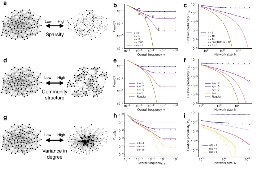
Figure 3: Network structure and the dynamics of complex contagions. For simplicity we omit the bar for $\bar{y}$ in all panels. a, Illustration of networks that are more (right) or less (left) sparse. b, Theoretical predictions (solid lines) and simulated results (for $N=10,000$; dots) for $P_{reach}(y)$ for networks of different sparsity. Theoretical predictions for the transition to the regime of negative and positive selection are shown as black or white arrows respectively. c, Theoretical predictions (solid lines) and simulated results (dots) for the fixation probability $P_{fix}(y)$ as a function of network size $N$. We show results for five values of $k$, corresponding to sparsity above (blue; top line), approximately on (purple; second line from top), and below (red; second line from bottom) the phase transitions allowing for global spread, as well as for a large value (yellow; bottom line) that approximates a fully-connected graph (dotted line). d, Illustration of networks with more (right) or less (left) community structure. e,f, Theoretical predictions (solid lines) and simulated results (dots) for $P_{reach}(y)$ (e) and $P_{fix}$ (f) for networks with different strengths of community structure. g, Illustration of networks with high (right) or low (left) variance in degree distribution. h,i, Theoretical predictions (solid lines) and simulated results (dots) for $P_{reach}(y)$ (h) and $P_{fix}$ (i) for networks with mean degree $k=10$ and standard deviation in degree distribution $\sigma_{k}=30$ for contagions with $\beta=0.1$ (h), $\beta=0.05$ (i), and three different values of $\alpha$ corresponding to initially positive, initially neutral, and initially negative selection on a regular graph with equal mean degree. Dotted lines show theoretical predictions for those equivalent regular graphs (i.e. with equal $k=10$ but $\sigma_{k}=0$). Large $\sigma_{k}$ decreases $P_{reach}$ for positive selection and increases $P_{reach}$ for negative selection. In both cases, the absolute effect of selection is lessened by higher degree variance. Parameters: $\alpha=1.0$, $\beta=0.1$ (b), $\alpha=0.4$, $\beta=0.04$ (c), $\alpha=0.88$, $\beta=0.1$, $m=k=20$ (e), $\alpha=0.2$, $\beta=0.025$, $m=k=20$ (f), $\alpha=(2.5,1.0,0.71)$ (h), $\alpha=(1.25,0.5,0.36)$ (i). All parameters correspond to positive frequency dependence and are chosen so that the curves’ distinguishing features are clearly visible within a reasonable range of magnitudes and computational budget. All line labels are ordered top to bottom in the legend in the same order as they appear in the plot itself. The dashed lines in (h-i) have the same top to bottom ordering as the corresponding solid lines.

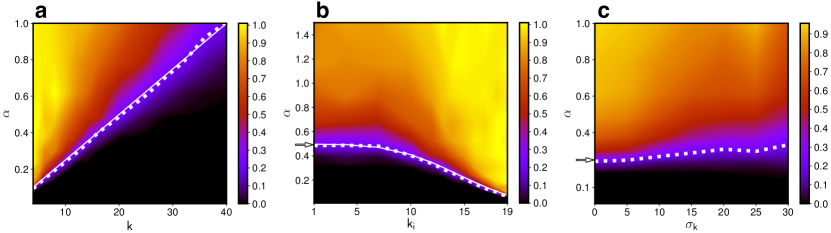
Figure 4: Phase transitions for complex contagions. a,b,c, Ratio of $P_{fix}$ on a network of size $N_{1}=50000$ to $P_{fix}$ on a network of size $N_{2}=2000$ for contagions with $\beta=0.025$, different values of $\alpha$ and varying sparsity (a), community structure ($k=m=20$) (b), or degree distributions ($k=10$) (c). Values close to one correspond to cases where $P_{fix}$ does not scale strongly with $N$, so global cascades are possible even in large networks. Solid white lines in (a,b) denote the theoretically predicted phase transition, and the thick dashed white line indicates an observed ratio of $1/5=\sqrt{N_{1}/N_{2}}$ (the empirical location of the phase transition). The theoretical value for (a) is found by evaluating $s(0)=0$ using equation Eq. 8. The theoretical value for (b) is found by numerically evaluating $s(\frac{m}{N})$ and finding where it is equal to zero given the parameters (See the sections on “Phase transitions” in [43] for details). In (b), the location of the phase transition approaches the regular random graph value (white arrow, can be read off for $k=20$ in panel (a)) as the network loses community structure and becomes regular random ($k_{i}\to\frac{m}{N}\approx 0$). In (c), the empirical phase transition also correctly approaches the theoretical prediction (regular graph limit, white arrow) as $\sigma_{k}\to 0$. Since wider degree distributions weaken the effect of selection, the “transition regime” becomes noticeably wider for large $\sigma_{k}$.

To gain insight into the effect of various aspects of network structure on the spread of complex contagions, we now apply the ideas of effective diffusion processes and selection regimes to contagions on several archetypical families of networks. One simple but critical aspect of network structure is that not all nodes are connected. To focus on the effects of this sparsity, we consider the spread of a contagion on a random regular graph, where each node is connected at random to exactly $k$ other nodes [51]. In such a network, each node will no longer see the “global” value $\bar{y}$, but rather some local value that reflects the fraction of its neighbors that happen to be type B. In principle, determining these local values of $y$ is a complicated problem. However, because the network is random, we expect no strong locality in how type B individuals are distributed, so the neighbors of each individual form an approximately random sample of size $k$ of the whole population. This no-locality (or “annealed”) [52, 53] approximation is related to the assumption that a large randomly connected network initially looks “locally tree-like” [9, 33] for a spreading contagion, but specifically ignores the fact that type B nodes are slightly more likely than chance to be connected to one another (this is because they can in reality only initially appear as a neighbor of another type B individual). The assumption of no locality contrasts with the case of a spatial network (e.g. a square lattice) where locality is fundamental to the network geometry (in this case the contagion becomes a front propagation problem and must be treated differently [54]). We confirm the accuracy of the no-locality assumption in Supplementary Fig 2. [43], and contrast it with the case of spatial networks in Supplementary Figs. 3 and 4 [43].

In our approximation (see “Sparse networks” in [43] for details), the distribution of $y$ as seen by a given individual with $k$ neighbors follows a Hypergeometric (approximately a Binomial for $k\ll N$) distribution with success probability $\bar{y}$ and $k$ trials:

$$y\sim\frac{1}{k}\text{Hypergeometric}(N,\bar{y}N,k)\;,$$

which implies $E_{A}[y]=\bar{y}$. In a simple contagion (with $f_{1/2}$ independent of $y$), only the first moment of the local distribution of $y$ appears in Eqs. 1 and 2. A simple contagion is thus unaffected by network sparsity. By contrast, higher moments appear in Eqs. 1 and 2 for a complex contagion with $y$-dependent $f_{1/2}(y)$. Due to discreteness in the connectivity (and thus the nonzero variance in the distribution of local $y$), some type A nodes will have more type B neighbors than others, and hence $E_{A}[y^{2}]>E_{A}[y]^{2}=\bar{y}^{2}$. Sparsity therefore increases $\text{Rate}_{A\to B}$ and $s(y)$ compared to the well mixed behavior Eq. 5 and enhances the spread of a complex contagion.

III.2 Results

Using the hypergeometric distribution over local $y$ and its moments, we can obtain the expectation values in Eqs. 1 and 2 and hence compute the effective selection $s(\bar{y})$ on this graph using Eq. 4. Specifically, we find that for large networks where $N\gg k$ (and assuming $\alpha,\beta\ll 1$),

$$s(\bar{y})=\alpha\left(\bar{y}+\frac{(1-\bar{y})}{k}\right)-\beta\;.$$ (8)

This reduces to the well-mixed solution $s(\bar{y})=\alpha\bar{y}-\beta$ as $k$ becomes large, but for small $k$ selection is significantly enhanced, as shown in Figure 2 (c). The intuition is that for small $k$, some nodes will by chance happen to have a higher fraction of type B neighbors than others due to local sampling fluctuations. Because the transition rates increase non-linearly with $y$, the increased positive selection on the few individuals that see high values of $y$ outweighs the effect of the reduced value of $y$ seen by individuals with fewer type B neighbors. While this effect is present for all $k$, it becomes stronger for smaller $k$ since the variance in the locally observed $y$ increases with smaller $k$.

The example of sparse regular networks illustrates several general patterns in our analysis. The distribution of type B individuals is influenced by the network structure and discreteness for any contagion process, but it is only for complex contagions that it affects selection and thus the spread.This happens through the higher moments of the distribution of local $y$, which only appear in Eqs. 1 and 2 if there is a frequency dependence of $f_{1/2}$, i.e. for a complex contagion. By contrast, as long as the first moment is unchanged from $\bar{y}$, a simple contagion is not affected by network structure (see “Simple contagion” in [43]).

Generally, for a given $\bar{y}$, structure influences how type B individuals are distributed during the contagion, which through Eqs. 1 and 2 interacts with the specific form of $f_{1/2}(y)$ to produce the effective selection strength $s(\bar{y})$. This determines regimes of selection and the overall behavior of the contagion. Moreover, $s(\bar{y})$ defines an effective diffusion process capturing the behavior of $\bar{y}(t)$, which we can easily solve using standard methods to obtain $P_{reach}(\bar{y})$, the fixation probability $P_{fix}$, properties of the temporal evolution [14], or any other quantities of interest. Thus we can reduce our problem to calculating the distribution of $y$ in the neighborhoods of type A and type B individuals at a given global value of $\bar{y}$. In general, $s$ at any point in time will depend on the full configuration of the type B individuals on the network. However, using key assumptions about the dynamics, we can often significantly reduce the degrees of freedom on which $s$ depends. In the above example, by assuming no locality and noting the random connectivity of the network, we reduced the complexity of the process to a single degree of freedom: $\bar{y}$.

Figure 3 b,c shows that our theory accurately predicts the results of numerical simulations of the process for various degrees of sparsity. Moreover, we show in Figure 3 b that the simple condition $N|S(y)-S(y^{*})|=1$ accurately predicts transitions between selection regimes. In particular, the black arrows are the predictions for transitioning from initially neutral selection at small $y$ to negative selection, which is visible on the log-log plot as a change from a straight line to a downward bending shape of $P_{reach}(y)$. The white arrows are the predictions for transitioning from the negative selection regime to the positive selection regime (which manifests visually as a transition from a downward bending trend to flat $P_{reach}(y)$.

While a precise treatment of the additional effects of locality is beyond the scope of this work, we can provide some intuition for its effects. Locality slightly increases the chances of the extreme outcomes of having zero type B neighbors as well as the chances of having many type B neighbors (see Supplementary Fig. 2 [43]). This is because type B nodes are created by definition only if they are initially in contact with another type B individual, so they are slightly more likely than chance to be found next to each other. They are also more likely than chance to be connected to each other in a locally “tree-like” structure [33]. Because the true distribution of $y$ is slightly wider than in our approximation, the variance is slightly higher and thus the effect on selection is slightly more positive than predicted. This explains the slight underestimation of $P_{reach}$ and $P_{fix}$ in Figure 3 by our approach. We have confirmed that these discrepancies disappear in a modified version of the simulation where node identities are shuffled on the graph at every time step (making the no locality assumption exactly true). As the specific form of the nonlinearity interacts with the distribution of $y$ through its higher moments, the differences in the distribution of $y$ compared to the no locality approximation could potentially lead to larger discrepancies between our theory and simulations for different nonlinearities. Nonetheless, the approximation allows us to build a quantitative and intuitive picture that captures important aspects of the true process.

IV Community based networks

IV.1 Approach

Next we consider the effect of community structure, where the impact of within-community locality is essential to the contagion dynamics. To analyze this effect, we consider random graphs that consist of randomly connected communities of $m$ individuals each. In particular, we assume every individual has exactly $k_{i}$ random connections within the community and $k_{e}$ outside of it, where $k_{i}+k_{e}\equiv k$. By tuning $k_{i}/k$, we can vary the strength of community structure. As $\frac{k_{i}}{k}\to 1$, we have very strong and cohesive communities, while $\frac{k_{i}}{k}\to\frac{m}{N}$ reduces to the case of a random regular graph of degree $k$.

We will provide a brief description of the approach, for more details we refer to “Community based networks” in [43]. To analyze the contagion on such a graph, we must understand how type B individuals distribute themselves across the network. For clarity, let use $z$ to denote the fraction of type B individuals within a given community. We are then interested in the distribution of the $z$ values, as seen across all communities in the network. Let us denote this distribution with $a(z)$, which gives the fraction of communities at a fixed value of $z$. Note that $z$ is discretized in units of $\frac{1}{m}$, and we have $\sum_{z}za(z)=\bar{y}$. Because the connections on the network are random within and between communities, we will assume that each node sees a random sample of size $k_{i}$ from within the community with its internal edges, and a random sample of size $k_{e}$ of the rest of the graph with its $k_{e}$ external edges. This is effectively a targeted version of the no-locality assumption: for the same reasoning as with the regular random graph, while the distribution of node types across communities $a(z)$ matters, the location of type B individuals in a given community does not, and neither does how the communities are shuffled for a fixed $a(z)$. We demonstrate the validity of our assumptions in Supplementary Fig. 2 [43]. This allows us to determine the distribution of $y$ as seen by a given node:

$$y=\frac{i_{i}+i_{e}}{k_{i}+k_{e}}\;,$$ (9)

where $i_{i}$ and $i_{e}$ are Hypergeometric random variables just like in the section on sparse networks representing the number of type B neighbors coming from edges internal to the community and external to it, respectively. That is,

$$i_{i} \sim (m-1,zm,k_{i})\;,$$ Hypergeometric

$$i_{e} \sim (N-m,N\bar{y}-zm,k_{e})\;,$$ Hypergeometric (10)

Intuitively, in addition to discreteness effects as before, the distribution of $y$ for a given node is now a weighted mixture between the $z$ of the community that the node is located in, and the global value of $\bar{y}$. It is now more clear how the distribution $a(z)$ will affect the local distribution of $y$ as seen by a given individual: if the distribution $a(z)$ is tightly centered around the global $\bar{y}$, we expect the overall results to be very similar to a regular random graph of degree $k$, i.e. no significant effect of community structure. On the other hand, if the distribution $a(z)$ has significant departures from $\bar{y}$, (for example, most communities could be either “full” or “empty” and only spend little time in between), most nodes will either see very high values of $y$ or very low because of the partial effect of $z$ (which is modulated by the community strength $\frac{k_{i}}{k}$). This increases the variance in the distribution of $y$ (without affecting its mean), which similarly to the case of the regular random graph will change the effective selection on the graph through the higher moments appearing in Eqs. 4, 1 and 2.

To find the distribution $a(z)$, we make the key assumption that for any given $\bar{y}$, the distribution of $y$ values seen within communities reaches a quasi-steady-state before $\bar{y}$ can change significantly across the whole graph. This distribution will depend on the connectivity of the network as well as the details of the transition probabilities. The steady-state approximation assumes that within-community dynamics are fast compared to global changes of $y$ across the whole network; we expect this to hold when selection is weak ($f_{1/2}(y)\ll 1$) and when communities are small and well-connected compared to the overall network.

If we assume that we know the distribution $a(z)$, we can use the definitions of the contagion dynamics together with our knowledge of how the individual types are distributed to determine the rate at which $z$ changes in each community. Specifically, the rate of change of $a(z)$ for each value of $z$ will depend on the number of type B and type A individuals in those communities ($mz$ and $m(1-z)$, respectively), as well as the rates at which individuals in communities of a given $z$ change types (which through Eq. 4 depend on their local distribution of $y$, which we can in turn obtain from Eqs. 9 and IV.1). These transitions change the value of $z$ for a given community and thus cause transition rates between entries of $a(z)$ for neighboring values of $z$. This allows us to write down a nonlinear dynamical system for the temporal evolution of $a(z)$. By numerically finding the steady state of this system subject to the normalization conditions $\sum_{z}a(z)=1$ and $\sum_{z}za(z)=\bar{y}$, we can compute the equilibrium distribution for $a(z)$ (this ultimately becomes a nonlinear algebraic system of equations that can be solved using zero-finding routines, see “Computing the equilibrium value of $a$” in [43]).

The equilibrium distribution for $a(z)$ then allows us to compute the local distribution of $y$ as seen by a given node by using Eqs. 9 and IV.1 and the law of total expectation to marginalize over $z$ using $a(z)$. We show that our approximations accurately predict this distribution of local $y$ in Supplementary Fig. 5 [43]. As in the case of regular networks, the local distribution of $y$ implies an effective selection strength $s(\bar{y})$ acting on the contagion (Figure 2 (d)). Overall, assuming that $a(z)$ is at equilibrium for any global $\bar{y}$ allows us to compute numerically an effective selection strength $s(\bar{y})$, which determines the behavior of the contagion. The agreement between our theoretical predictions and numerical simulations are shown in Figure 3 (d-f).

IV.2 Results

When community strength is weak ($\frac{k_{i}}{k}\to\frac{m}{N}$), the equilibrium distribution of $a(z)$ is narrowly peaked around the global value of $\bar{y}$. In this case, each community simply behaves like a random sample of nodes from the overall network, and we have the same behavior as for the regular random network. By contrast, when communities are cohesive ($\frac{k_{i}}{k}\to 1$), the equilibrium distribution of $a(z)$ has the same mean, but is now more peaked at the extremes of $z=0$ and $z=1$. This “U-shaped” distribution of $z$ means that type B individuals are concentrated in just a few communities. The resulting distribution of local $y$ as seen by individuals is also more peaked at the extremes, since individuals see mostly edges from within their own communities, and those communities are either mostly type A or mostly type B. This wider distribution of local $y$ enhances the spread of the contagion (for the same reason that higher variance in local $y$ enhances selection for the regular random graph).

We provide here some intuition for the transition of $a(z)$ between the narrowly peaked and U-shaped regimes as a function of $\frac{k_{i}}{k}$. In [43] section “Continuum approximation” we provide a more quantitative justification based on an effective diffusion process for $z$ in a given community for fixed $\bar{y}$. For high $k_{i}$, the U-shaped distribution of $z$ arises because the many connections within a community can “conduct” influence between the types and thus cause rapid fluctuations of $z$ within the community, but only slow fluctuations between communities. The rate of fluctuations are fastest when there are approximately equally many type B and type A individuals in a community. By contrast, fluctuations are slow when nearly all the nodes within a community have the same type. The values of $z$ within a community (which are subject to random diffusion) will therefore spend most of their time at extreme values of $z\to 0$ or $z\to 1$. This intuition is confirmed in that we observe a critical level of community strength $\frac{k_{i}}{k}$ above which the equilibrium distribution of $z$ within a community turns from a narrow distribution (concentrated around the global $\bar{y}$ across the whole network) to a U-shaped distribution (same mean, but concentrated at the extreme values), as shown in Supplementary Fig. 5 [43]. The resulting variance in $y$ as seen by individuals is high, and selection is enhanced. Intuitively, it is much easier for the contagion to randomly reach a “critical mass” of popularity within a single community and experience positive selection there, compared to across the whole network. The contagion simply fixes one community at a time, as visualized in Supplementary Fig. 6 [43] as well as Supplementary Videos 1-3 [43]. These effects also explain our observations on the role of clustering and community strength on real social networks in Figure 1. It is important to note that the unequal distribution of type B individuals among communities (just like the broader distribution of $y$ in sparse networks) is again a feature purely of the network structure and arises with or without complex contagion. However, it is only in the former case that this distribution has an effect on the spread.

V Graphs with variable degree distribution

V.1 Approach

Finally, we consider graphs with variable degree distributions and otherwise random connectivity. We present a brief description of the approach and refer to “Networks with degree distributions” in [43] for details. Intuitively, there are competing effects and it is not immediately clear what the net impact of varying degree distributions should be on the spread of the contagion. On the one hand, high degree type B nodes are able to convert many other nodes once they are converted, but they are harder to convert themselves. On the other hand, it is easier to convert low degree nodes to type B for the same reason that low $k$ increases selection for the random regular graph, but those individuals in turn will influence fewer neighbors. Given a fixed average degree, it is not clear what effect a greater variance in degree will have.

In the case of non-regular graphs, the degrees $k$ of the nodes are distributed according to a degree distribution $P(k)$ (which for regular graphs has zero variance, an assumption that we now relax). For a given individual of degree $k$ on the graph, we will also need the distribution over the degrees $k^{\prime}$ of their neighbors $P(k^{\prime}|k)$. While this neighbor degree distribution can in principle be arbitrary, we expect it without further information to have the form $P(k^{\prime}|k)\sim P(k^{\prime})k^{\prime}$ since each node of degree $k^{\prime}$ has $k^{\prime}$ edges to which one can be connected (any departure from this distribution is called “assortativity”).

For networks with a nontrivial distribution $P(k)$, it is no longer possible to calculate a selection strength $s$ that depends only on $y$. Instead, we must work with the fraction of nodes of each degree $k^{\prime}$ that are type B, $y_{k^{\prime}}$. This requires an explicit analysis of the fraction of type B individuals for each degree $k^{\prime}$, which leads to a high-dimensional diffusion process. Note that this still reduces the effective degrees of freedom significantly compared to the true process on the network, but not as much as in the regular graph case where we only track a single degree of freedom.

We can solve this multi-dimensional diffusion process using the no-locality approximation, i.e. assuming that nodes of degree $k$ see a random sample of all other nodes on the graph. The probability distribution of the value of $y$ seen by a given individual will now depend on the degrees $k^{\prime}$ of the individual’s neighbors through $y_{k^{\prime}}$ (the probability of a given node being type B is $y_{k}^{\prime}$ and depends on $k^{\prime}$). The degrees of the neighbors $k^{\prime}$ in turn depend on the neighbor degree distribution $P(k^{\prime}|k)$. Using the law of total expectation, we find the simple and intuitive result that nodes of degree $k$ see a distribution of $y$ identical to that for a $k$-regular random graph, with the global frequency $\bar{y}$ replaced by the “effective frequency”

$$z_{k}=\sum_{k^{\prime}}P(k^{\prime}|k)y_{k^{\prime}};.$$ (11)

Using this distribution of the local value of $y$ as seen by a given node of degree $k$, we can use the same approach as for the regular graphs to determine the rates Eq. 1 and thus obtain the diffusion process. This time, however, there is such a process for each population of $NP(k)$ nodes at each value of $k$ and they are coupled together through the mixing across degrees in Eq. 11. This coupled high-dimensional diffusion process in $y_{k}$ space must therefore be solved numerically.

V.2 Results

To vary both the mean and variance of the degree distribution continuously, we consider graphs where the degree of each node is drawn from a Gamma distribution with mean $k$ and variance $\sigma_{k}$. Specifically, in order to illustrate the effect of wide degree distributions, in Figure 3 (g-i) we compare graphs with $\sigma_{k}=0$ (i.e. regular random graphs as studied before) to networks with high degree variance ($\sigma_{k}=30$) and equal mean degree. We consider regimes that on a regular graph with would consist of initial positive selection ($s(0)>0$), initial neutral selection ($s(0)=0$) and initial negative selection followed by positive selection ($s(0)<0$). Our theoretical predictions show excellent agreement with the full numerical simulations. Note that for graphs with high degree variance, the behavior of $P_{reach}(y)$ becomes “less extreme”, whether selection is positive or negative (we find lower $P_{reach}$ in the case of positive selection and higher $P_{reach}$ in the case of initial negative selection). Overall, we find that broader degree distributions dampen the effects of selection (whether positive or negative) on the contagion, both for simple and for complex contagions. Another effect is the consistent suppression of the contagion for very low $y$ (see Figure 3 (h)), which is enhanced for distributions with significant degree correlations (see Supplementary Figure 8 [43]). We give intuition and a derivation for this effect in [43] (see the sections “Suppression at low $y$” and “Impact of the neighbor degree distribution”). We also verify the soundness of our modeling approach by comparing the predicted local distribution of $y$ to observations in Supplementary Figure 7 [43] showing close agreement.

VI Phase transitions

Whenever it is possible to compute an $s(y)$, our framework implies a simple condition under which the contagion can spread globally with finite probability even in arbitrarily large networks (i.e. global cascades are possible, see “Phase transitions” in [43]): the width of a region of negative $s(y)$ around $y=0$ must scale as $N^{-\gamma}$, with $\gamma\geq 1$. That is, the contagion must need to tunnel through at most a finite number of individuals to reach a frequency above which it is positively selected. Otherwise, the process encounters negative selection and is exponentially unlikely to spread globally for large $N$. Using Eq. 8 and setting $s(0)=0$, this leads to the critical sparsity $k_{crit}=\frac{1}{y_{n}}=\frac{\alpha}{\beta}$ below which global contagion is possible (Figure 4 (a)). Note that this result is in line with previous work considering locally tree-like connectivity [9, 33] and has a simple intuitive interpretation: each individual that sees at least one type B neighbor has $s(y)=s(\frac{1}{k})\approx\frac{\alpha}{k}-\beta$. If this minimum selection is nonnegative, the contagion can spread globally.

For community-based networks, we find that the effective selection strength has $s(0)=-\beta$, but jumps higher as $y\to\frac{m}{N}$ (see Figure 2 (d)). Global contagion is possible provided that $s(\frac{m}{N})\geq 0$, because in that case the contagion only needs to overcome a fixed size negative selection regime of size at most $m$ that does not scale with $N$. Numerically, we find this implies a critical community strength $k_{i}/k$ above which complex contagions are able to spread globally by appearing popular and reaching critical mass in one community at a time, even though they do not have critical mass on the global network (Figure 4 (b)). This is in line with our initial simulations of contagions on real social networks Figure 1 (c-e).

VII Discussion

These results demonstrate quantitatively how interactions between non-linear adoption probabilities and network structure influence the dynamics and outcomes of complex contagions by modulating the effects of selection and stochasticity. A central idea was the use of targeted approximations (e.g. no locality on random networks, local vs. global equilibration time scales on community based networks) to reduce the contagion to an effective diffusion process on a lower dimensional space ($y$ for regular networks, $y_{k}$ for random graphs with degree distributions, and the space of per-community $z$ for community based networks) and hence obtain its statistical properties. This allows us to understand the behavior of both large and small contagions, as well as the emergence of global cascades. These results help explain why the spread of even initially unpopular ideas and opinions can be enhanced both by overall sparsity as well as by cliques and other forms of community structure. They also show that in contrast to simple contagions (where the existence of highly-connected individuals always enhances spread), broad degree distributions dampen both positive and negative selection for complex contagions and hence have more subtle effects.

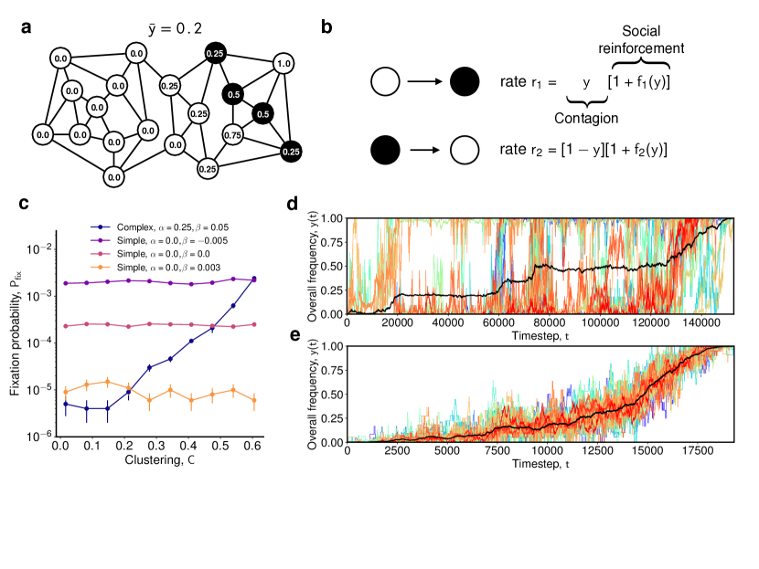
Figure 1: Model and simulations on real social networks. a, We model a complex contagion on a network where each individual can be type B or type A. We denote the global frequency of type B individuals as $\bar{y}$. Each node sees a potentially different local fraction $y$ of type B neighbors (node labels). b, Transition rates between type B and type A individuals occur at rates $r_{1}$ and $r_{2}$; the form of $f_{1/2}(y)$ determines the non-linear adoption probabilities in complex contagions. c, Simulations on networks of variable clustering derived by swapping pairs of edges in a Facebook network[49] ($N=4039$, $k=43$) show that the spread of complex (but not simple) contagions are highly sensitive to clustering. The line increasing with clustering is the complex contagion. The three flat lines correspond to simple contagions and are ordered top to bottom as in the legend. d,e, Example frequency trajectories for contagions that fixed in our simulations. Each colored line shows the frequency within a given community as detected by a standard community detection algorithm [55], while the black line shows overall frequency $\bar{y}$. If the community structure is strong, the contagion fixes one community at a time, rapidly gaining and maintaining local popularity which helps the spread (d, Clustering $C=0.6$). If the community structure is weaker (but still detectable [55]), the contagion instead spreads uniformly across the entire network (e, $C=0.2$). This is much less likely, so the fixation probability $P_{fix}$ is lower in this case. Simulations assume $f_{1}(y)=\alpha y$, $f_{2}(y)=\beta$, $\alpha=0.25$, and $\beta=0.05$.

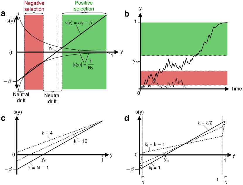
Figure 2: Selection and genetic drift in complex contagions. For simplicity we omit the bar for $\bar{y}$ in all panels. a, The condition $N|s(y)|y=1$ distinguishes regimes where contagion dynamics are dominated by genetic drift, negative selection, or positive selection (this is an approximation to the exact condition $N|S(y)|=1$, see SI). b, A contagion can spread globally if it reaches high enough frequency to be positively selected; this may require “tunneling” through a regime of negative selection at lower frequencies. c,d, Sparsity (c) and community structure (d) can change the shape of $s(y)$ and hence alter the contagion dynamics.

References

- Zhou et al. [2015] C. Zhou, Q. Zhao, and W. Lu, Impact of repeated exposures on information spreading in social networks, PloS one 10, e0140556 (2015).
- Pentland [2014] A. Pentland, Social physics: How good ideas spread-the lessons from a new science (Penguin, 2014).
- Christakis and Fowler [2013] N. A. Christakis and J. H. Fowler, Social contagion theory: examining dynamic social networks and human behavior, Statistics in medicine 32, 556 (2013).
- Keeling [1999] M. J. Keeling, The effects of local spatial structure on epidemiological invasions, Proceedings of the Royal Society of London B: Biological Sciences 266, 859 (1999).
- Weng et al. [2013] L. Weng, F. Menczer, and Y.-Y. Ahn, Virality prediction and community structure in social networks, Scientific reports 3, 2522 (2013).
- Nematzadeh et al. [2014] A. Nematzadeh, E. Ferrara, A. Flammini, and Y.-Y. Ahn, Optimal network modularity for information diffusion, Physical review letters 113, 088701 (2014).
- Montanari and Saberi [2010] A. Montanari and A. Saberi, The spread of innovations in social networks, Proceedings of the National Academy of Sciences 107, 20196 (2010).
- Granovetter [1978] M. Granovetter, Threshold models of collective behavior, American journal of sociology 83, 1420 (1978).
- Watts [2002] D. J. Watts, A simple model of global cascades on random networks, Proceedings of the National Academy of Sciences 99, 5766 (2002).
- Borge-Holthoefer et al. [2013] J. Borge-Holthoefer, R. A. Baños, S. González-Bailón, and Y. Moreno, Cascading behaviour in complex socio-technical networks, Journal of Complex Networks 1, 3 (2013).
- López-Pintado [2008] D. López-Pintado, Diffusion in complex social networks, Games and Economic Behavior 62, 573 (2008).
- Bauch and Galvani [2013] C. T. Bauch and A. P. Galvani, Social factors in epidemiology, Science 342, 47 (2013).
- Centola and Macy [2007] D. Centola and M. Macy, Complex contagions and the weakness of long ties, American journal of Sociology 113, 702 (2007).
- Eckles et al. [2018] D. Eckles, E. Mossel, M. A. Rahimian, and S. Sen, Long ties accelerate noisy threshold-based contagions, Available at SSRN 3262749 0 (2018).
- Pinheiro et al. [2018] F. L. Pinheiro, V. V. Vasconcelos, and S. A. Levin, Consensus and polarization in competing complex contagion processes, arXiv preprint arXiv:1811.08525 0 (2018).
- Hébert-Dufresne and Althouse [2015] L. Hébert-Dufresne and B. M. Althouse, Complex dynamics of synergistic coinfections on realistically clustered networks, Proceedings of the National Academy of Sciences 112, 10551 (2015).
- Guilbeault et al. [2018] D. Guilbeault, J. Becker, and D. Centola, Complex contagions: A decade in review, Complex spreading phenomena in social systems , 3 (2018).
- Centola [2018] D. Centola, How behavior spreads (Princeton University Press, 2018).
- Mønsted et al. [2017] B. Mønsted, P. Sapieżyński, E. Ferrara, and S. Lehmann, Evidence of complex contagion of information in social media: An experiment using twitter bots, PloS one 12, e0184148 (2017).
- Romero et al. [2011] D. M. Romero, B. Meeder, and J. Kleinberg, Differences in the mechanics of information diffusion across topics: idioms, political hashtags, and complex contagion on twitter, in Proceedings of the 20th international conference on World wide web (2011) pp. 695–704.
- State and Adamic [2015] B. State and L. Adamic, The diffusion of support in an online social movement: Evidence from the adoption of equal-sign profile pictures, in Proceedings of the 18th ACM Conference on Computer Supported Cooperative Work & Social Computing (2015) pp. 1741–1750.
- Sprague and House [2017] D. A. Sprague and T. House, Evidence for complex contagion models of social contagion from observational data, PloS one 12, e0180802 (2017).
- Steinert-Threlkeld [2017] Z. C. Steinert-Threlkeld, Spontaneous collective action: Peripheral mobilization during the arab spring, American Political Science Review 111, 379 (2017).
- Centola [2015] D. Centola, The social origins of networks and diffusion, American Journal of Sociology 120, 1295 (2015).
- Ugander et al. [2012] J. Ugander, L. Backstrom, C. Marlow, and J. Kleinberg, Structural diversity in social contagion, Proceedings of the National Academy of Sciences 109, 5962 (2012).
- Guilbeault and Centola [2021] D. Guilbeault and D. Centola, Topological measures for identifying and predicting the spread of complex contagions, Nature communications 12, 1 (2021).
- Bakshy et al. [2015] E. Bakshy, S. Messing, and L. A. Adamic, Exposure to ideologically diverse news and opinion on facebook, Science 348, 1130 (2015).
- Toole et al. [2012] J. L. Toole, M. Cha, and M. C. González, Modeling the adoption of innovations in the presence of geographic and media influences, PloS one 7, e29528 (2012).
- Traag [2016] V. A. Traag, Complex contagion of campaign donations, PloS one 11, e0153539 (2016).
- Krapivsky et al. [2011] P. L. Krapivsky, S. Redner, and D. Volovik, Reinforcement-driven spread of innovations and fads, Journal of Statistical Mechanics: Theory and Experiment 2011, P12003 (2011).
- Dodds and Watts [2004] P. S. Dodds and D. J. Watts, Universal behavior in a generalized model of contagion, Physical review letters 92, 218701 (2004).
- Dodds and Watts [2005] P. S. Dodds and D. J. Watts, A generalized model of social and biological contagion, Journal of theoretical biology 232, 587 (2005).
- Dodds et al. [2011] P. S. Dodds, K. D. Harris, and J. L. Payne, Direct, physically motivated derivation of the contagion condition for spreading processes on generalized random networks, Physical Review E 83, 056122 (2011).
- Centola [2010] D. Centola, The spread of behavior in an online social network experiment, science 329, 1194 (2010).
- Lehmann and Ahn [2018] S. Lehmann and Y.-Y. Ahn, Complex spreading phenomena in social systems (Springer, 2018).
- Hui et al. [2018] P.-M. Hui, L. Weng, A. S. Shirazi, Y.-Y. Ahn, and F. Menczer, Scalable detection of viral memes from diffusion patterns, in Complex Spreading Phenomena in Social Systems (Springer, 2018) pp. 197–211.
- Gleeson [2008] J. P. Gleeson, Cascades on correlated and modular random networks, Physical Review E 77, 046117 (2008).
- Pastor-Satorras and Vespignani [2001] R. Pastor-Satorras and A. Vespignani, Epidemic spreading in scale-free networks, Physical review letters 86, 3200 (2001).
- House and Keeling [2011] T. House and M. J. Keeling, Insights from unifying modern approximations to infections on networks, Journal of The Royal Society Interface 8, 67 (2011).
- Leventhal et al. [2015] G. E. Leventhal, A. L. Hill, M. A. Nowak, and S. Bonhoeffer, Evolution and emergence of infectious diseases in theoretical and real-world networks, Nature communications 6, 6101 (2015).
- Pagel et al. [2019] M. Pagel, M. Beaumont, A. Meade, A. Verkerk, and A. Calude, Dominant words rise to the top by positive frequency-dependent selection, Proceedings of the National Academy of Sciences 0, 201816994 (2019).
- Allen [2008] L. J. Allen, An introduction to stochastic epidemic models, in Mathematical epidemiology (Springer, 2008) pp. 81–130.
- [43] J. Kates-Harbeck, See supplemental material at [url will be inserted by publisher] for additional details and derivations supporting the analytical results; for a discussion of the relationship of our work with epidemiological models; as well as for a description of the numerical and algorithmic methods used. The supplemental material includes Refs. [44, 45, 46, 47, 48].
- Desai and Fisher [2007] M. M. Desai and D. S. Fisher, Beneficial mutation–selection balance and the effect of linkage on positive selection, Genetics 176, 1759 (2007).
- Salganik et al. [2006] M. J. Salganik, P. S. Dodds, and D. J. Watts, Experimental study of inequality and unpredictability in an artificial cultural market, science 311, 854 (2006).
- Newman [2012] M. E. Newman, Communities, modules and large-scale structure in networks, Nature physics 8, 25 (2012).
- Yang et al. [2016] Z. Yang, R. Algesheimer, and C. J. Tessone, A comparative analysis of community detection algorithms on artificial networks, Scientific reports 6, 30750 (2016).
- Arman et al. [2021] A. Arman, P. Gao, and N. Wormald, Fast uniform generation of random graphs with given degree sequences, Random Structures & Algorithms 59, 291 (2021).
- Leskovec and Krevl [2014] J. Leskovec and A. Krevl, SNAP Datasets: Stanford large network dataset collection, http://snap.stanford.edu/data (2014).
- Ewens [2012] W. J. Ewens, Mathematical Population Genetics 1: Theoretical Introduction, Vol. 27 (Springer Science & Business Media, 2012).
- Wormald et al. [1999] N. C. Wormald et al., Models of random regular graphs, London Mathematical Society Lecture Note Series 0, 239 (1999).
- Derrida and Pomeau [1986] B. Derrida and Y. Pomeau, Random networks of automata: a simple annealed approximation, EPL (Europhysics Letters) 1, 45 (1986).
- Galstyan and Cohen [2007] A. Galstyan and P. Cohen, Cascading dynamics in modular networks, Physical Review E 75, 036109 (2007).
- Tanaka et al. [2017] H. Tanaka, H. A. Stone, and D. R. Nelson, Spatial gene drives and pushed genetic waves, Proceedings of the National Academy of Sciences 114, 8452 (2017).
- Raghavan et al. [2007] U. N. Raghavan, R. Albert, and S. Kumara, Near linear time algorithm to detect community structures in large-scale networks, Physical review E 76, 036106 (2007).