Effects of the environment on the multiplicity properties of stars in the STARFORGE simulations

Abstract

Most observed stars are part of a multiple star system, but the formation of such systems and the role of environment and various physical processes is still poorly understood. We present a suite of radiation-magnetohydrodynamic simulations of star-forming molecular clouds from the STARFORGE project that include stellar feedback with varied initial surface density, magnetic fields, level of turbulence, metallicity, interstellar radiation field, simulation geometry and turbulent driving. In our fiducial cloud the raw simulation data reproduces the observed multiplicity fractions for Solar-type and higher mass stars, similar to previous works. However, after correcting for observational incompleteness the simulation under-predicts these values. The discrepancy is likely due to the lack of disk fragmentation, as the simulation only resolves multiples that form either through capture or core fragmentation. The raw mass distribution of companions is consistent with randomly drawing from the initial mass function for the companions of $>1\,\mathrm{M}_{\rm\sun}$ stars, however, accounting for observational incompleteness produces a flatter distribution similar to observations. We show that stellar multiplicity changes as the cloud evolves and anti-correlates with stellar density. This relationship also explains most multiplicity variations between runs, i.e., variations in the initial conditions that increase stellar density (increased surface density, reduced turbulence) decrease multiplicity. While other parameters, such as metallicity, interstellar radiation, and geometry significantly affect the star formation history or the IMF, varying them produces no clear trend in stellar multiplicity properties.

1 Introduction

Stars form in highly clustered environments (Lada & Lada, 2003), and both young and older stellar populations have a significant fraction of multiples, which are defined as bound systems of two or more stars. The likelihood of a star being in a multiple is observed to increase monotonically with mass (see reviews of Duchêne & Kraus 2013; Lee et al. 2020 and references therein). It is generally understood that multiple systems form either during the star-forming phase of the parent cloud, where the dominant channels are the fragmentation of a protostellar core (Goodwin et al., 2004) or disk (Adams et al., 1989), or through dynamical evolution during the dissolution of the cluster (Kouwenhoven et al., 2010; Parker & Meyer, 2014).

The detailed multiplicity properties of a stellar system are characterized by several metrics, which are usually defined as a function of the mass of the most massive star, i.e., the primary, in the system. One commonly measured property is the mass ratio $q$ of the secondary to the primary mass. For Solar-type stars the mass ratio distribution is statistically consistent with a flat distribution (Raghavan et al., 2010) for most of the companion mass range, except for two features: a lack of brown dwarf-scale companions (“brown dwarf desert”, see e.g., Kraus et al. 2008) and an excess of companions at near-unity mass ratio (“twins”, see El-Badry et al. 2019). Other metrics concern the orbits of the companions, which can be characterized with the orbital period/semi-major axis and orbital eccentricity distributions. The semi-major axis distribution of Solar-type stars is well-described by a lognormal distribution that peaks around 100 AU (Raghavan et al., 2010). The eccentricity distribution $f(e)$ for companions of Solar-type stars with separations $>50\,\mathrm{AU}$ follows $f(e)\approx 1.2e+0.4$ and in general eccentricity increases with orbital period (Tokovinin & Kiyaeva, 2016).

There has been significant theoretical effort to explain these observations, mainly through detailed hydrodynamical simulations. Simulations of star cluster formation show good agreement with observed multiplicity statistics (Bate, 2009a, 2012; Krumholz et al., 2012; Lee et al., 2019; Li et al., 2018)) using different combinations of physical processes. Unfortunately the dynamic range of simulations is unavoidably limited, leading to either insufficient resolution to resolve close binary formation (e.g., Mathew & Federrath, 2021) or low number statistics due to the small cloud size (e.g., Rohde et al., 2021). Thus pinpointing the key physics is challenging.

Note that most simulations only follow the star-forming phase of the cluster evolution, so they in fact predict the multiplicity of stars close to formation. Both observations (Duchêne, 1999; Kraus et al., 2008, 2011; Tobin et al., 2016, 2022) and simulations suggest that stars are born in complex, multiple systems that dynamically evolve (e.g., ejection of stars) causing multiplicity to drop (Goodwin & Kroupa 2005; Goodwin et al. 2007; Kaczmarek et al. 2011) and the period/separation distribution to shift to shorter periods/ closer separations (Kroupa 1995; Marks et al. 2011). This can be understood as the result of wide-separation binaries becoming unbound due to either internal dynamical evolution or by interacting with external tidal fields, the latter of which also increases the average binding energy between the remaining stars. In general, dynamical interactions cause strongly bound binaries to be even more bound (i.e., “harden”), while the separation of weakly bound companions increases (Heggie, 1975).

To date most simulations have attempted to recover the observed multiplicity properties without conducting a detailed parameter study on how their initial conditions might affect multiplicity (see Lee et al. 2019 for an exception). In this work we present the first comprehensive analysis of how cloud properties affect stellar multiplicity properties. We use simulations from the STAR FORmation in Gaseous Environments (STARFORGE) project that include all relevant physical processes of star formation. These radiation-magnetohydrodynamic (RMHD) simulations achieve a dynamic range in mass resolution that allow us to simulate the detailed evolution of molecular clouds while following the formation of individual low-mass stars (see Grudić et al. 2021a, henceforth referred to as the Methods Paper). In this study we analyze a set of runs with varied initial cloud surface density, level of turbulence, magnetic field strength, metallicity and interstellar radiation field and compare them to a fiducial run with parameters representing a typical Milky Way molecular cloud (similar to Grudić et al. (2022), henceforth referred to as Paper I). We focus on the evolution of multiplicity properties from the onset of star formation until cloud disruption.

The paper is structured as follows: §2 provides a brief overview of the code (for details on numerical methods as well as tests see the Methods Paper) and the initial conditions of the runs. We present our results for the fiducial run in §3 and compare them with observations. In §4 we explore how multiplicity properties change in response to variations in the initial parameters. An analysis of the clustering properties, the star formation history and the initial mass functions of these runs are presented in Guszejnov et al. (2022a) and Guszejnov et al. (2022b), henceforth referred to as Paper II and Paper III respectively. We discuss the implications of our results to observations and future work in §5. Finally, we present our conclusions in §6.

2 Numerical Methods

2.1 The STARFORGE simulations

For this work we utilize simulations from the STARFORGE project, which are run with the GIZMO code. A full description and presentation of the STARFORGE methods including a variety of tests and algorithm details are given in the Methods Paper. We only briefly summarize the key points here. Note that in this work we use the same physics modules as Paper I and our fiducial run uses identical initial conditions as the run presented there. Readers familiar with the STARFORGE simulation methods should skip ahead to §2.2 where we define the various metrics used in this study.

2.1.1 Physics

We simulate star-forming clouds with the GIZMO code (Hopkins, 2015) using the Lagrangian meshless finite-mass (MFM) method for magnetohydrodynamics (Hopkins & Raives, 2016), assuming ideal MHD. Individual stars in the simulations are represented by sink particles . Once they form they follow the protostellar evolution model from Offner et al. (2009), extended past the main sequence by the mass-loss and stellar lifetime prescriptions presented in Methods Paper.

The presented STARFORGE runs utilize the radiative cooling and thermochemistry module from Hopkins et al. (2022) that contains detailed metallicity-dependent cooling and heating physics, including recombination, thermal bremsstrahlung, metal lines, molecular lines, fine structure and dust collisional processes. The cooling module self-consistently solves for the internal energy and ionization state of the gas. The simulations co-evolve the gas, dust, and radiation temperature self-consistently, including the stellar luminosity in various bands accounting for photon transport, absorption and emission using dust opacity. In addition to local sources (i.e. stars) we include an external heating source at the boundary of the simulation domain that represents the interstellar radiation field (ISRF).

The simulations account for the dominant stellar feedback processes, including protostellar jets, radiative feedback from both protostars and main sequence stars, stellar winds and supernovae. See Paper I and the Methods Paper for details on the numerical implementations.

2.1.2 Initial Conditions & Parameters of Clouds

We use cloud initial conditions (ICs) identical to those presented in Paper III, so we only give a short summary here.

We generate our initial conditions using MakeCloud (Grudić & Guszejnov, 2021). Our default IC geometry is the “Sphere” where we initialize the cloud as a homogeneous sphere near thermal pressure equilibrium with a low density ambient medium. We apply an initial random velocity field with a power spectrum of $E_{k}\propto k^{-2}$ with amplitude set by the $\alpha_{\rm turb}\equiv 5\sigma^{2}R_{\mathrm{cloud}}/(3GM_{0})$ turbulent virial parameter. The cloud is initially threaded by a uniform magnetic field $B_{z}$ whose strength is set by the normalized mass-to-flux ratio $\mu$. There is no external driving in “Sphere” simulations.

We also run a simulations using the “Box” geometry, a periodic box with externally driven turbulence whose side length $L_{\mathrm{box}}$ gives the box a volume equal to that of a Sphere cloud model of similar mass. The box is initialized with a uniform density and stationary gas and then “stirred” for five global freefall times $\left(t_{\mathrm{ff}}\equiv\sqrt{\frac{3\pi}{32G\rho_{0}}}\right)$, to achieve saturated MHD turbulence. An important difference between the Sphere and Box runs is that in the latter case the magnetic field is enhanced by dynamo action during the stirring phase (e.g., Federrath et al. 2011; Tricco et al. 2016).

Table 1 shows the target parameters for the runs we present in this paper. The input parameters are the cloud mass $M_{0}$, size $R_{0}$, turbulent virial parameter $\alpha_{\mathrm{turb}}$, normalized magnetic mass-to-flux ratio $\mu$, metallicity $Z$ and the energy density of the ISRF $e_{\mathrm{ISRF}}$ (note that initial temperature is set by the ISRF). Similar to Paper I our fiducial cloud satisfies the observed Milky Way cloud mass-size relation (e.g. Larson 1981; Lada & Dame 2020, specifically assuming $\Sigma\equiv M_{\mathrm{0}}/\uppi R_{\mathrm{cloud}}^{2}=63\mathrm{M}_{\rm\sun}\,\mathrm{pc}^{-2}$). The cloud is marginally bound ($\alpha_{\mathrm{turb}}=2$) and begins in thermal equilibrium with the ISRF. The initial gas metallicity is assumed to be equal to the solar value. For the initial magnetization we assume $-E_{\mathrm{mag}}/E_{\mathrm{grav}}=0.01$, which translates to $\mu=4.2$. The STARFORGE simulations we use have a mass resolution of $\Delta m=10^{-3}\,\mathrm{M}_{\rm\sun}$, making the mass function incomplete stars with masses below $0.1\,\mathrm{M}_{\rm\sun}$, which we omit from our analysis (see Paper III for a convergence test). Sphere runs continue until stellar feedback quenches star formation and subsequently disrupts the cloud (see Figure 1). In the case of the Box runs the periodic boundary conditions trap both radiation and cloud material, so we terminate the run when the box becomes saturated by stellar radiation.

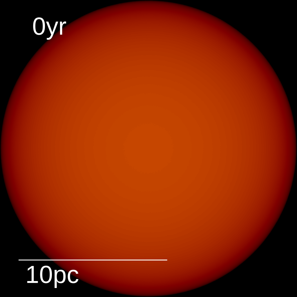
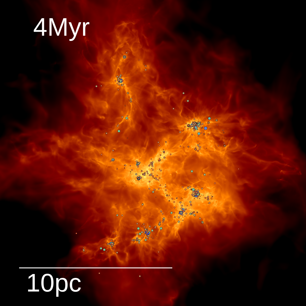
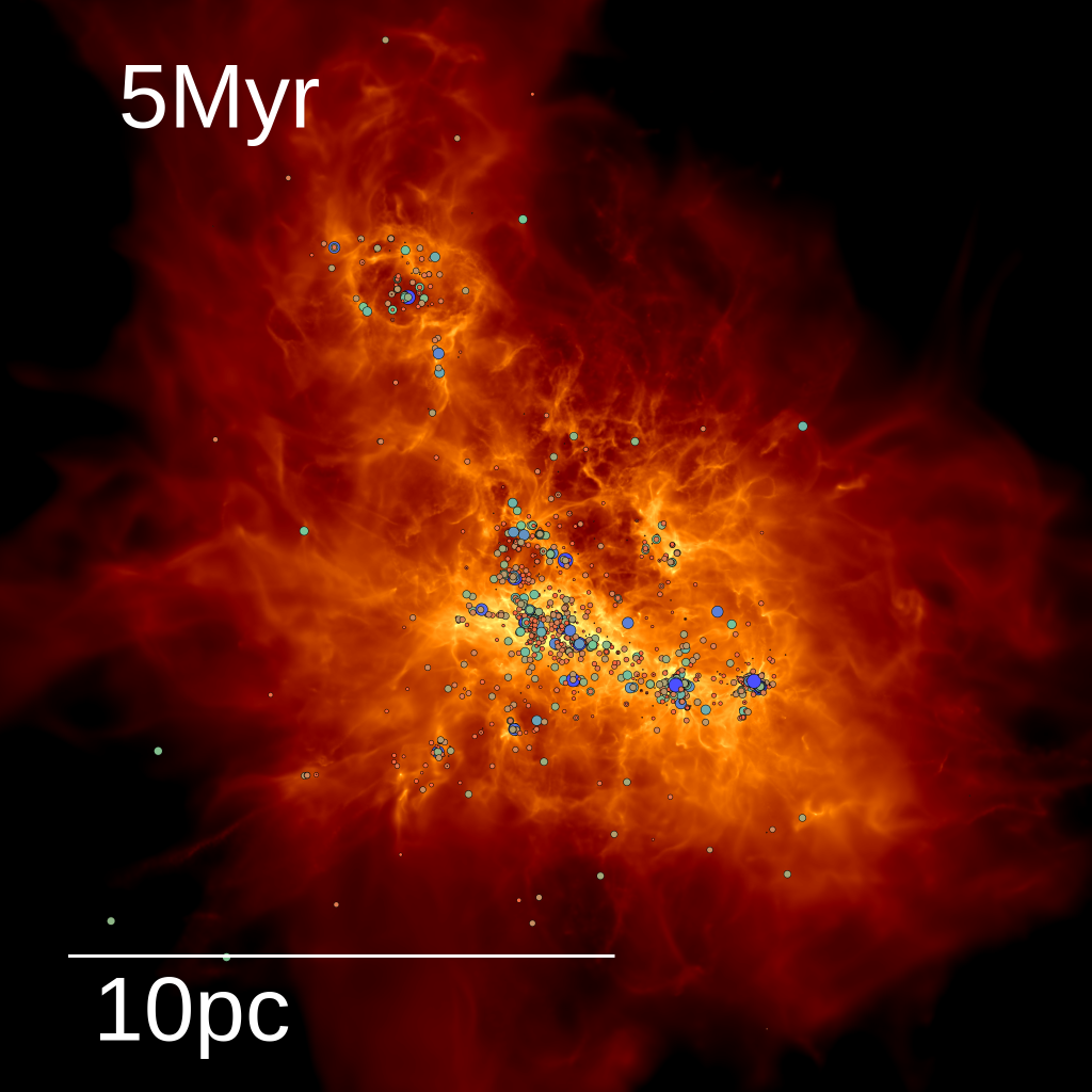
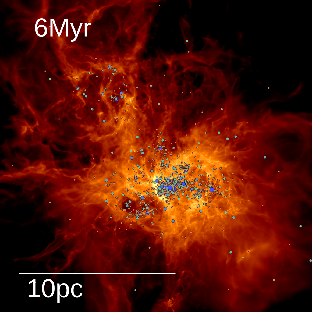
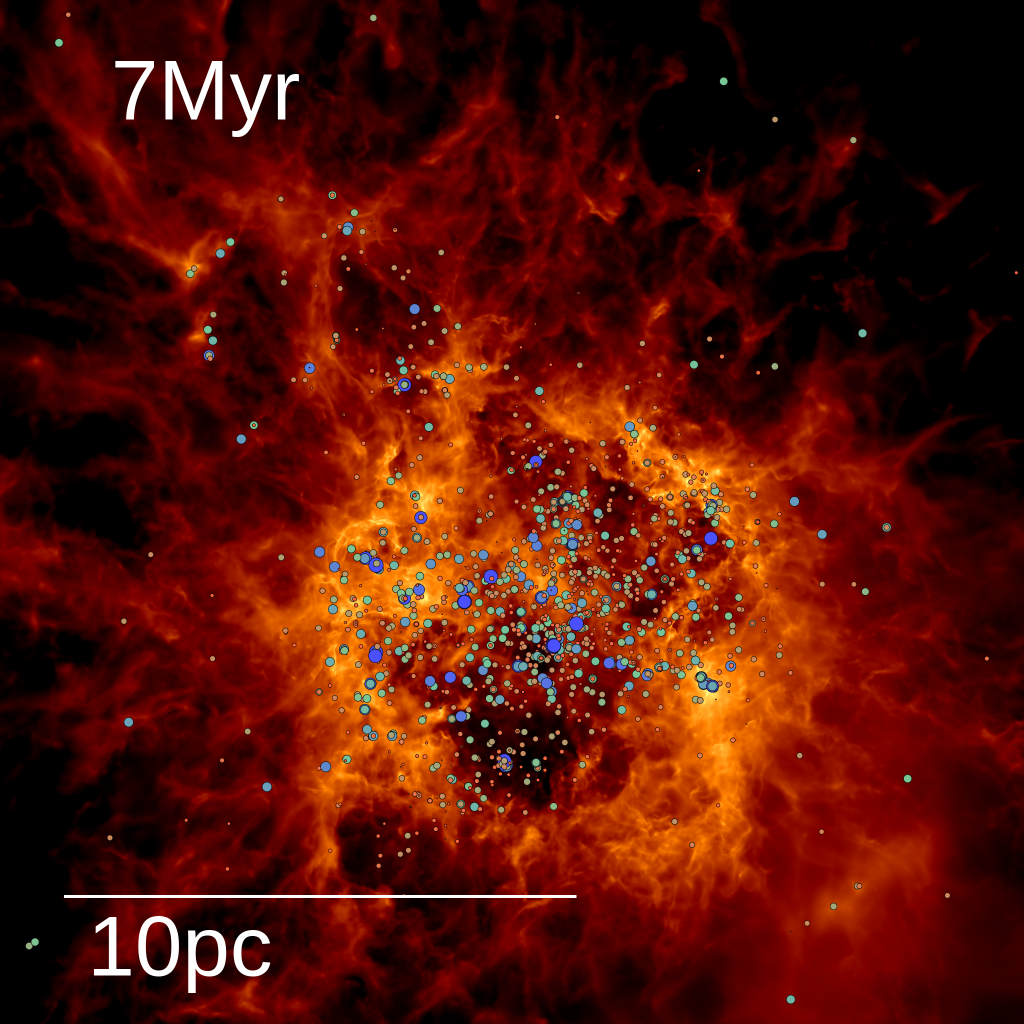
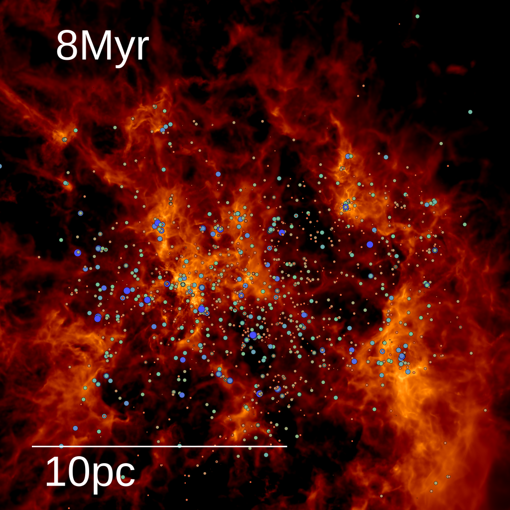
Figure 1: Surface density maps for M2e4 (our fiducial run), which is an $M_{0}=2\times 10^{4}\,\mathrm{M}_{\rm\sun}$ mass cloud resolved with $M_{0}/\Delta m=2\times 10^{7}$ initial gas cells (see Table 1) at different times, from the beginning of the simulation until cloud disruption. The color scale is logarithmic, and the circles represent sink particles (stars) that form in high-density regions where fragmentation can no longer be resolved. The size of the circles increases with mass, and their color changes from red ($M\sim 0.1\,\mathrm{M}_{\rm\sun}$), green ($M\sim 1\,\mathrm{M}_{\rm\sun}$) to blue ($M\sim 10\,\mathrm{M}_{\rm\sun}$). This simulation resolves a dynamic range from $\sim\!\mathrm{20\,pc}$ down to $\sim\!\mathrm{30\,AU}$ and evolves until stellar feedback quenches star formation and disrupts the cloud.

Physics label	Thermodynamics	MHD	Protostellar Jets	Stellar Radiation	Stellar Winds & SNe
C_M_J_RT_W	Non-isothermal, RHD (C)	Ideal (M)	Included (J)	Included (RT)	Included (W)

	Input Parameters								Derived Parameters								Results
Cloud label	$\frac{M_{0}}{\mathrm{M}_{\rm\sun}}$	$\frac{R_{\mathrm{cloud}}}{\mathrm{pc}}$	$\frac{L_{\mathrm{box}}}{\mathrm{pc}}$	$\alpha_{\mathrm{turb}}$	$\mu$	$\frac{Z}{Z_{\mathrm{\odot}}}$	$\frac{e_{\mathrm{ISRF}}}{e_{\mathrm{ISRF,solar}}}$	$\frac{\sigma}{\mathrm{km/s}}$	$\alpha_{\mathrm{th}}$	$\alpha$	$\mathcal{M}_{\rm A}$	$\beta$	$\alpha_{\mathrm{B}}$	$\frac{M_{\rm Jeans}}{M_{0}}$	$\frac{M_{\rm sonic}}{M_{0}}$	$\frac{M_{\Phi}}{M_{0}}$	SFE [%]	$t_{\mathrm{disrupt}}/t_{\mathrm{ff}}$
M2e4 (fiducial)	$2\times 10^{4}$	10		2	4.2	1	1	3.2	0.008	2.03	10	0.78	0.02	$3\times 10^{-3}$	$7\times 10^{-5}$	0.1	$\mathrm{9\pm 0.3}$	$\mathrm{1.6\pm 0.2}$
M2e4 (Box)	$2\times 10^{4}$		16	2	4.2	1	1	3.2	0.008	2.03	10	0.78	0.02	$3\times 10^{-3}$	$7\times 10^{-5}$	0.1
M2e4_R3	$2\times 10^{4}$	3		2	4.2	1	1	5.8	0.008	2.02	10	0.23	0.02	$5\times 10^{-4}$	$7\times 10^{-6}$	0.1	14	2.0
M2e4_R30	$2\times 10^{4}$	30		2	4.2	1	1	1.9	0.02	2.04	10	2.3	0.02	$1\times 10^{-2}$	$6\times 10^{-4}$	0.1	1	1.7
M2e4_a1	$2\times 10^{4}$	10		1	4.2	1	1	2.3	0.008	1.03	10	0.78	0.02	$3\times 10^{-3}$	$4\times 10^{-5}$	0.1	11	1.2
M2e4_a4	$2\times 10^{4}$	10		4	4.2	1	1	4.5	0.008	4.03	10	0.78	0.02	$3\times 10^{-3}$	$1\times 10^{-4}$	0.1	4	2.1
M2e4_mu1.3	$2\times 10^{4}$	10		2	1.3	1	1	3.2	0.008	2.21	3.1	0.078	0.2	$3\times 10^{-3}$	$7\times 10^{-5}$	0.4	7	2.0
M2e4_mu0.4	$2\times 10^{4}$	10		2	0.42	1	1	3.2	0.008	4.01	3.1	0.0078	2	$3\times 10^{-3}$	$7\times 10^{-5}$	4	5	2.2
M2e4_ISRF10	$2\times 10^{4}$	10		2	4.2	1	10	3.2	0.008	2.03	10	0.78	0.02	$3\times 10^{-3}$	$7\times 10^{-5}$	0.1	10	1.6
M2e4_ISRF100	$2\times 10^{4}$	10		2	4.2	1	100	3.2	0.008	2.03	10	0.78	0.02	$3\times 10^{-3}$	$7\times 10^{-5}$	0.1	11	1.3
M2e4_Z01	$2\times 10^{4}$	10		2	4.2	0.1	1	3.2	0.008	2.03	10	0.78	0.02	$3\times 10^{-3}$	$7\times 10^{-5}$	0.1	7	1.1
M2e4_Z001	$2\times 10^{4}$	10		2	4.2	0.01	1	3.2	0.008	2.03	10	0.78	0.02	$3\times 10^{-3}$	$7\times 10^{-5}$	0.1	4	1.6

Table 1: Simulations used in this paper described with STARFORGE label conventions. Top: Physics modules included, see Methods Paper for details on the individual physics modules. Bottom: Initial conditions of our simulated clouds, where $M_{0}$, $R_{\mathrm{cloud}}$, $\alpha_{\mathrm{turb}}$. $\mu$, $Z$ and $e_{\mathrm{ISRF}}$ are the initial cloud mass, size, virial parameter, mass to magnetic flux ratio, metallicity and the energy density of the ISRF, respectively. Note these runs explicitly evolve the radiation field so the initial gas-dust temperature is set by the ISRF. We also report the initial 3D turbulent velocity dispersion $\sigma$, thermal virial parameter $\alpha_{\mathrm{th}}$, total virial parameter $\alpha$, Alfvén Mach number $\mathcal{M}_{\rm A}$, plasma $\beta$, magnetic virial parameter $\alpha_{\mathrm{B}}$, as well as the relative Jeans, sonic and magnetic mass scales (note that these are all defined assuming as 10 K gas temperature, see §2 in Guszejnov et al. 2020 for definitions). Note that Box runs have slightly different initial parameters (e.g., Mach number, virial parameter) due to the non-exact scaling of the turbulent driving, so the values shown here are the target values that are to be reached at the end of the initial turbulent driving phase of 5 crossing times. In the last two column we show the final star formation efficiency ($\mathrm{SFE}=M_{*}/M_{0}$) and the disruption time for the Sphere runs, see Paper III for detailed star formation histories. For the fiducial run these columns also show the standard variations between the three runs that were run with different initial turbulent realizations.

2.2 Multiplicity calculation and metrics

To derive multiplicity statistics in our simulation snapshots we first need to identify bound systems. We do so by using the hierarchical algorithm introduced by Bate (2012), which has the following steps:

1. Calculate the binding energy between all pairs of stars.

2. Find the most bound pair (i.e., having the lowest total energy) and replace it with a single point mass with the same total mass and momentum, located at the center of mass of the removed pair.

3. Recursively repeat steps 1 and 2 until no more bound stars are left, with the exception that we do not combine pairs if the resulting bound aggregate would consist of more than 4 individual stars. If such an aggregate is the most bound pair at any point, we proceed to the next most bound pair, terminating if no other bound pair exists.

Using the above algorithm we produce a list of bound systems. For each star in these systems we assign one of the following labels:

1. Unbound: The star is not bound to any other stars.

2. Primary: The star is the most massive (primary) star of a multiple star system.

3. Non-primary: The star is part of a multiple star system, but it is not the primary star.

Following the definitions from the literature (e.g., Duchêne & Kraus 2013) we introduce a set of multiplicity metrics (summarized in Table 2), starting with the multiplicity fraction $\mathrm{MF}$:

$$\mathrm{MF}\equiv\frac{B+T+Q}{S+B+T+Q},$$ (1)

where $S,B,T,Q$ are the number of single, binary, triple, quadruple systems whose primary star is in mass bin $M$. Similarly we introduce the companion frequency $\mathrm{CF}$:

$$\mathrm{CF}\equiv\frac{B+2T+3Q}{S+B+T+Q},$$ (2)

which is the average number of companions in systems with primary mass of $M$. Due to the relatively small number of high mass stars in the simulations ($\sim 30$ have $>10\,\mathrm{M}_{\rm\sun}$ out of $\sim 2000$ stars), the uncertainty of $\mathrm{MF}$ and $\mathrm{CF}$ can be significant in high mass bins. We estimate the errors using a Bayesian method where we assume the number of multiples and companions follow a binomial and Poisson distribution respectively, see Appendix A for details.

For companions we characterize the companion separation as the semi-major axis $a$ with respect to the primary using the well-known two-body solution to the Kepler problem that yields

$$a=\frac{GM_{1}M_{2}}{2E_{\mathrm{total}}},$$ (3)

where $G$ is the gravitational constant, $M_{1}$ and $M_{2}$ are the masses of the primary and companion stars, and $E$ is the kinetic+gravitational energy of the system. Similarly, we calculate the orbital period $P$ as

$$P=2\mathrm{\pi}\sqrt{\frac{a^{3}}{G(M_{1}+M_{2})}}.$$ (4)

To compute these quantities for higher order systems we adopt the orbit and mass of the highest level subsystem that contains the chosen star but not the primary, see Figure 2 for an illustration. For each orbit we also calculate the corresponding eccentricity

$$e=\sqrt{\frac{h^{2}}{aG(M_{1}+M_{2})}-1},$$ (5)

where $h$ is the specific relative angular momentum of the two-body system.

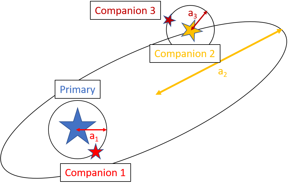
Figure 2: Cartoon illustration of the definition of orbits for each companion in a quadruple system. When calculating the semi-major axes or orbital periods for a companion, we take the orbit of the highest level subsystem that contains the chosen star but not its companion. We substitute the properties of these subsystems into Eqs 3-4. To calculate the semi-major axis or eccentricity distribution in §3-4 we count the semi-major axis between all subsystems. Here, this would mean the orbits with semi-major axes of $a_{1}$, $a_{2}$ and $a_{3}$.

Property	Definition
$M_{p}$	Mass of the primary (i.e., most massive) star in the system
$q\equiv M/M_{p}$	Mass ratio of a companion to the primary
$\mathrm{MF}$	Multiplicity fraction for stars of $M_{p}$ primary mass, see Eq. 1
$\mathrm{CF}$	Companion frequency for stars of $M_{p}$ primary mass, see Eq. 2
$a$	Semi-major axis of companion’s orbit, see Eq. 3
$P$	Orbital period of the companion, see Eq. 4
$e$	Eccentricity of companion’s orbit, see Eq. 5

Table 2: List of multiplicity properties used throughout the paper along with their definition.

To compare these metrics with observations we apply two corrections to the “raw” multiplicity properties of the simulations. First, all companions with mass ratio $q<0.1$ are ignored, as most observations are incomplete in this regime, see Moe & Di Stefano (2017) henceforth referred to as MDS17. We note that the exact choice of the cut-off $q$ value can significantly affect the companion frequency at the high mass end of the IMF, since there are many Solar-type companions around $>10\,\mathrm{M}_{\rm\sun}$ stars in our simulations. When specifically comparing the properties of simulated and observed Solar-type stars, we account for observational incompleteness by discarding shorter period companions ($\mathrm{Log}P<4.5$, or $a<30\,\mathrm{AU}$) for which observations are incomplete for $q<0.5$ and low-$q$ longer period binaries ($5.9<\mathrm{Log}P<6.7$, or $150<a/\mathrm{AU}<400$), which are only detectable for $q>0.2$ (see Figure 28 in MDS17). The second correction we apply removes all short-lived companions from the distribution, i.e., stars that have only been companions to their primaries for $t_{\rm comp}<100\,\mathrm{kyr}$ or have not yet completed two orbits. This correction removes binary assignments that are the result of chance alignments between stars (i.e., cases where the pairwise comparison considers two stars bound but they are not when accounting for all interactions), see §3 for details. Source confusion is likely only important in crowded regions, and indeed, we find that this correction has a relatively minor effect on the statistics. Note that we report the “raw” simulation values unless specified otherwise.

Finally, we also examine the multiplicity properties of young stellar objects (YSOs). Observed YSOs are classified according to their spectral energy distributions (Dunham et al., 2014), which requires radiative transfer post-processing (e.g., Offner et al., 2012). Instead, we take a simpler approach and define YSOs in the simulation as stars (sink particles) that are younger than 0.5 Myr, as 0.5 Myr is approximately the Class 0 + Class I lifetime (Dunham et al., 2014).

3 Multiplicity properties for the fiducial cloud

We run our fiducial cloud (M2e4) until star formation is quenched, and the cloud is fully disrupted by stellar feedback (see Figure 1). We identify star systems in all snapshots of the run using the method outlined in §2.2. Unless stated otherwise we show multiplicity properties at the end of the simulation, when star formation has quenched and the cloud has been fully disrupted.

Figure 3: Basic multiplicity properties at the end of the simulation in the fiducial run (M2e4) with a grey shaded region showing the mass range potentially affected by the $0.1\,\mathrm{M}_{\rm\sun}$ completeness limit of the simulations. Left: Fraction of stars in different boundedness categories. Middle & Right: Multiplicity fraction ($\mathrm{MF}$) and companion frequency ($\mathrm{CF}$) as a function of primary stellar mass, showing the raw simulation values (solid) and the distributions after removing temporary companions, low mass-ratio companions and both. Shaded regions show the 1-$\sigma$ uncertainties, which are estimated using Eqs. 8-10 for $\mathrm{MF}$ and $\mathrm{CF}$ respectively. Observed values are taken from the review of Offner et al. (2022). For an analysis of trends see §3 in the main text.

The left panel of Figure 3 shows the fraction of stars in different boundedness categories (see §2.2) as a function of mass. As expected we find that massive stars ($>5\,\mathrm{M}_{\rm\sun}$) are more likely to be primary stars. We find that, up to companion masses of $\sim$ $10~{}M_{\odot}$, 20% of stars are companions to more massive primary stars. These statistics derive from the fact that most high-mass stars are in multiple systems, while most low-mass stars are not. The middle and right panels of Figure 3 show that the multiplicity fraction ($\mathrm{MF}$) and companion frequency ($\mathrm{CF}$) increase with the primary mass and are qualitatively similar to the observed values. Note for stars with masses below $1\,\mathrm{M}_{\rm\sun}$ both the $\mathrm{MF}$ and $\mathrm{CF}$ are affected by the $0.1\,\mathrm{M}_{\rm\sun}$ completeness limit of the simulation; the simulation does not resolve brown dwarfs. Removing short-lived companions has a mild effect on both $\mathrm{MF}$ and $\mathrm{CF}$. Applying an observationally-motivated $q>0.1$ cut-off, however, significantly reduces both the $\mathrm{MF}$ and $\mathrm{CF}$ for high-mass stars. This is because many high-mass stars in the simulations have Solar-type companions,such that the system mass ratio falls just below the cut-off. Overall, we find that after corrections the simulations produce qualitatively similar but significantly lower values than those observed for both $\mathrm{MF}$ and $\mathrm{CF}$.

3.1 Companion properties

Observations find the distribution of the companion mass ratio $q$ is mostly flat for Solar-type stars, except for a peak at near-equal masses (Raghavan et al., 2010; Offner et al., 2022). Figure 4 shows that in our simulation the distribution is not flat and exhibits a peak at $q\sim 0.2$. Comparing with the normalized stellar mass function of the simulation, i.e., the IMF, we find that the companion mass ratio distribution for Solar-type stars is consistent with random sampling from the IMF. After applying a correction for observational incompleteness of short period, low mass ratio companions (based on MDS17) the distribution becomes flatter with a marginal peak at $q\sim 0.2$. Note that this marginal peak is dominated by low mass ratio, short-period companions so the significance of the peak strongly depends on the estimated observational completeness limit, which MDS17 estimated to be 25%. After these corrections the distribution is qualitatively consistent with the observed trend, except for the lack of peak at unity mass ratio.

Figure 4: Distribution of the companion mass ratio $q$ for Solar-type stars in the fiducial run, using a similar notation to Figure 3, where we account for observational incompleteness reported in MDS17. Bars show the Poisson error of the distributions in key bins. For a fixed primary mass each $q$ value corresponds to a stellar mass scale, so we plot the $<1\,\mathrm{M}_{\rm\sun}$ part of the stellar mass distribution (IMF, dashed line). We also show the observations for Solar-type binaries from Raghavan et al. (2010). A grey shaded region shows the mass ratio range potentially affected by the $0.1\,\mathrm{M}_{\rm\sun}$ completeness limit of the simulation. Overall the $q$-distribution before corrections is consistent with random sampling the IMF (dashed line) and only shows significant differences after removing low $q$ value companions. After all corrections are applied the distribution is much closer to the observed flat trend, with a significant absence of near-equal mass companions.

Figure 5 shows the period/semi-major axis distribution for all stars, as well as for Solar-type and massive ($>5\,\mathrm{M}_{\rm\sun}$) stars only. In all cases we find a peak close to the gravitational softening length ($\sim 20\,\mathrm{AU}$), below which gravitational forces are artificially weakened. Above this value the number of companions declines with distance. Note that removing temporary companions significantly reduces the number of wide binaries, while removing low-mass ratio companions affects all scales. Note that in the case of Solar-type stars removing $q<0.1$ companions have little effect as we ignore all brown dwarfs in the simulation as they are below the completeness limit of the simulations presented in this work. However, observations of Solar-type and lower mass stars are incomplete for higher values of $q$ (Offner et al., 2022). Fig. 5 also shows the result if we also account for observational incompleteness of Solar-type stars for $q<0.5$ companions with $<30\,\mathrm{AU}$ separations. After these corrections, the simulation qualitatively agrees with observations from MDS17 for wide binaries, but the pile-up at the gravitational softening scale, which is likely numerical, prevents a detailed comparison (e.g., comparing the statistical significance of the apparent peak at 100 AU for Solar-type stars).

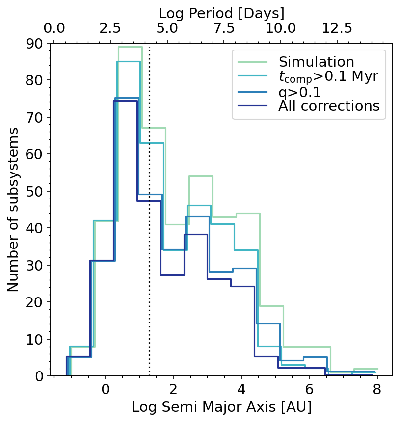
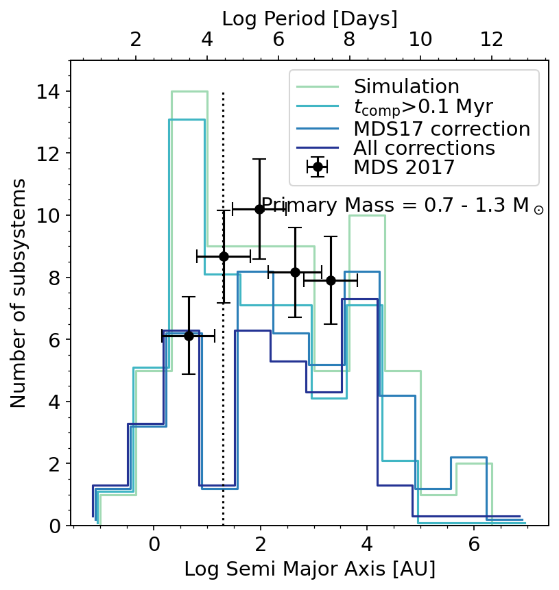
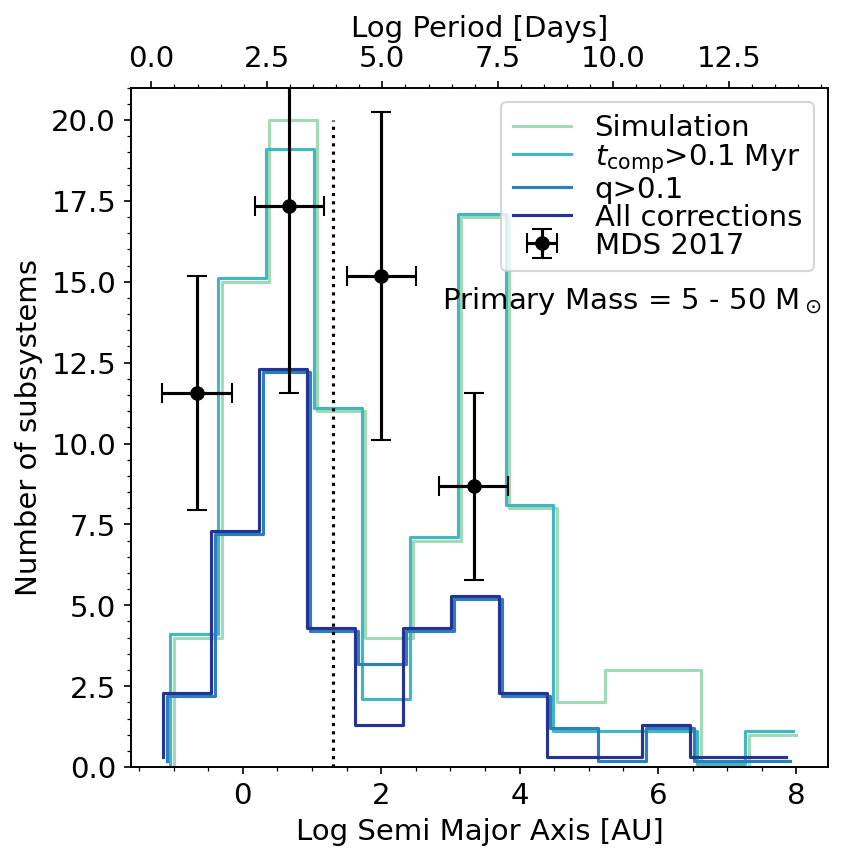
Figure 5: Left: Semi-major axis/orbital period distribution for star systems in the fiducial run (M2e4), using the same notation as Figure 3. A vertical line represents the 20 AU gravitational softening length of the simulation. Middle & Right: Same but for Solar-type and massive ($>5\,\mathrm{M}_{\rm\sun}$) primaries only, also showing the corresponding observations from MDS17. Note that for Solar-type stars we account for observational incompleteness based on MDS17.

In addition to the semi-major axis distribution, it is instructive to see the separation distribution between primaries and companions, which we define as the instantaneous 3D distance between the pair positions. The stars, particularly just after formation, are not on stable orbits with a well-defined semi-major axis and pair separations and may evolve rapidly (Offner et al., 2010; Lee et al., 2019) as shown in Figure 6. We compare the separation at formation between primaries and their companions with their separations at the end of the simulation. The former quantity reflects the initial conditions and characteristics of the mechanism by which the multiples form. Figure 7 shows the distributions for both separation metrics for massive ($>5\,\mathrm{M}_{\rm\sun}$) and lower mass ($<2\,\mathrm{M}_{\rm\sun}$) primaries. We find that most companions in the simulations formed between 1000 and 10000 AU from their primaries, which is the expectation for multiples formed via turbulent fragmentation (Fisher, 2004; Offner et al., 2010, 2016; Guszejnov et al., 2017). As a result of dynamical interactions most of these companions end up with much closer separations than their initial birth separation (see Figure 6). A significant fraction of companions migrate inwards until they reach scales at which gravitational softening impacts the dynamics, creating a peak in the distribution near the gravitational softening length. There is no clear trend in this behavior with regards to the companion mass ratio $q$: massive companions are as likely to “spiral in” as lower mass ones. Like prior numerical studies, we find that the separation evolution happens on a relatively short timescale of $<0.5\,\mathrm{Myr}$. Note that a few companions appear to have initial separations of $\lesssim 10^{2}\,\mathrm{AU}$. Due to the snapshot time increment ($\approx 7\,\mathrm{kyr}$), we don’t have the separations at the moment of formation and, consequently, these short distances likely represent early rapid dynamical evolution, rather than formation on these scales. Note that if the simulation included the formation of multiples from unstable disks, we would expect to see a larger number of companions forming at such short separations.

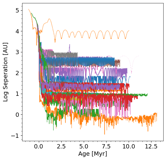
Figure 6: Separation of companions to their primary stars for a small sample of systems in the fiducial run as a function of the age of the bound system (note that the stars can form before the system becomes bound, hence the negative time values). Note that simulation snapshots are $\Delta t_{\mathrm{snap}}\approx 7\,\mathrm{kyr}$ apart, distorting the orbits of low separation companions. Overall we find that most companions form at larger distances ($\sim 10^{4}\,\mathrm{AU}$) and become bound almost immediately, then reach a stable orbit within $\sim 0.5\,\mathrm{Myr}$.

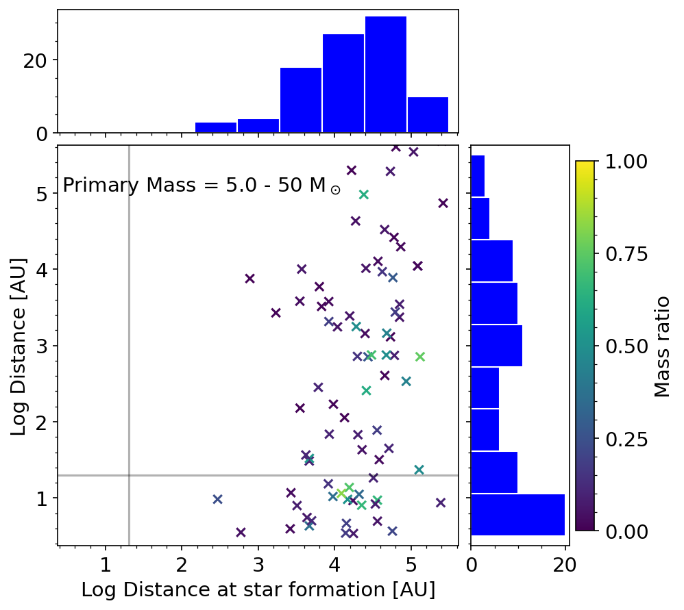
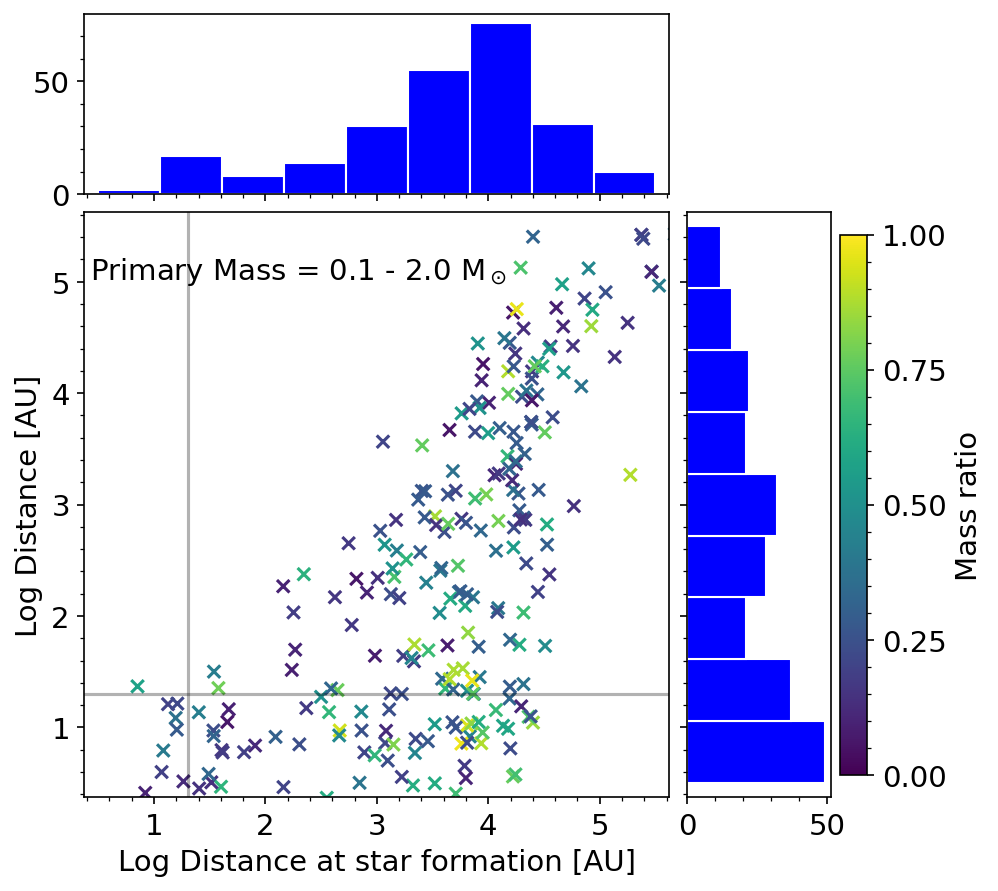
Figure 7: Separation between primary and companions in the fiducial simulation at the snapshot just after the stars form and at the end of the simulation. Results are shown separately for high mass ($>5\,\mathrm{M}_{\rm\sun}$, left) and lower mass ($<2\,\mathrm{M}_{\rm\sun}$, right) primary stars. The symbols in the main scatter plot are colored according to the companion mass ratio $q$ in the system at the end of the simulation. The distributions of the individual metrics is shown above their respective axes. A horizontal line show the gravitational softening length of the simulation, which is also the exclusion radius of sink particles (i.e., no stars can form closer than this) denoted by a vertical line. There are still a few stars that appear to have formed at shorter distances, but this is just an artifact of us relying on discrete snapshots of the simulation ($\Delta t_{\mathrm{snap}}\approx 7\,\mathrm{kyr}$). Note that we are showing the data after having applied the corrections for both low mass ratio and temporary companions.

In addition to the semi-major axis we calculate the eccentricity of each orbit. In Figure 8 we compare our results with the observations of Tokovinin & Kiyaeva (2016), who examined companions of Solar-type stars with $>50\,\mathrm{AU}$ separation, which is above the $\sim 20\,\mathrm{AU}$ gravitational softening length of the simulation. We find good agreement for all eccentricity values with the raw data. However applying all corrections leads to a deficit of companions in the $0.4<e<0.8$ range.

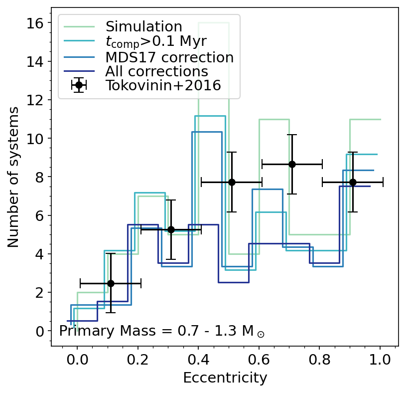
Figure 8: Distribution of the companion eccentricities for Solar-type stars in the fiducial run, using a similar notation to Figure 3, where we account for observational incompleteness reported in MDS17. We also show the observations for Solar-type stars from Tokovinin & Kiyaeva (2016). Overall the eccentricity distribution in the simulation is consistent with observations before corrections, but show a lack of companions at $e\sim 0.7$ after corrections.

The simulation tracks the angular momentum accreted by sink particles (stars), allowing us to analyse the spin alignment between stars and their companions. Note that the simulation does not allow stars to lose angular momentum via outflows or magnetic braking, so this total accreted angular momentum is significantly higher than the angular momentum of stars. Additionally, sink particles accrete angular momentum material from larger spatial scales than what may be actually accreted at the stellar surface, potentially leading to an overestimation of the accreted angular momentum. Nevertheless, the direction of the accreted angular momentum is a reasonable proxy for the direction of the stellar spin. Figure 9 shows the distribution of the angle between the spins of the primary star and its companions for both high ($>5\,\mathrm{M}_{\rm\sun}$) and lower mass primaries ($<2\,\mathrm{M}_{\rm\sun}$). We find that in both cases companions are not randomly oriented, but instead are preferentially aligned with their primaries, a potential sign that these multiples formed via core fragmentation, however prior work found a significantly weaker preference for spin alignment (Lee et al., 2019). However, massive primaries have a wider angle distribution, i.e., their spin is less likely to be aligned with that of their companions, which can be explained either by massive stars acquiring companions that formed in different regions or by the fact that massive stars accrete from a gas reservoir much larger than the initial core they form in.

Figure 9: Distribution of the misalignment angle between primaries and companions for high mass ($>5\,\mathrm{M}_{\rm\sun}$, left) and lower mass ($<2\,\mathrm{M}_{\rm\sun}$, right) primary stars, using the same notation as Figure 3. We also show the distribution expected from randomly aligned companions. Overall, companions tend to be more aligned with their primaries compared to a random distribution, while massive stars exhibit slightly more misalignment.

In Figure 10 we compare the primordial spin misalignment angle with the final value obtained at the end of the simulation. Taking the at-formation misalignment between companion and primary would yield similar results to random alignment as the spin direction of sink particles changes rapidly during the initial accretion. That is why we define primordial misalignment as the angle when the mass of the companion exceeds the mass scale of brown dwarfs ($0.08\,\mathrm{M}_{\rm\sun}$). Although companions tend to be aligned with their primary at both times, the primordial misalignment is closer to random. This is due to companions that accrete simultaneously with their primary star, bringing their spins closer to alignment.

Figure 10: Misalignment angle between primaries and companions in the fiducial simulation at the snapshot just after the stars form and at the end of the simulation. The primordial misalignment angle is calculated at the time when the mass of the companion exceeds $0.08\,\mathrm{M}_{\rm\sun}$. The symbols and colorbar are set identical to those in Figure 7. Companions are preferentially aligned even in the early, primordial stage, and become even more aligned by the time star formation ends.

3.2 Time evolution of multiplicity properties

Observations suggest that multiplicity evolves through dynamical interactions, such that over time systems lose members. Figure 11 shows the evolution of the $\mathrm{MF}$ for Solar-type stars in the fiducial run that have stopped accreting. We find a general decreasing trend, where Solar-type stars are much more likely to be primaries at the start of star formation than at later times. To produce this trend Solar-type stars must lose their companions as they age, or stars born at later times must have lower multiplicity. Figure 12 shows the formation rate of Solar-type stars and their multiplicity as a function of age. Note that Figure 11 and Figure 12 concern slightly different stellar populations: Figure 11 looks at Solar-type stars that have stopped accreting, while Figure 12 follows the multiplicity of stars throughout their lifetime. The $\mathrm{MF}$ remains roughly constant as the stars age, but the $\mathrm{CF}$ decreases. This means that trinary and quaternary systems containing Solar-type stars lose some companions over time but are unlikely to lose their last companion. This implies that most stars that form in a multiple system (e.g., not the earliest forming ones), stay in a multiple system. This result is consistent with prior numerical studies (e.g., Lee et al., 2019) and will hold as long as the initial fraction of high-order systems is low and stellar densities are not too high. These changes, however, are relatively minor compared to the differences in both the $\mathrm{MF}$ and $\mathrm{CF}$ between stars born at different times. We find that among the first Solar-type stars that form about 40% are primaries; among the last ones to form only 20% are.

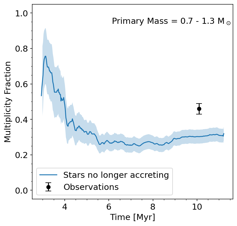
Figure 11: Multiplicity fraction of Solar-type stars that are no longer accreting (i.e., will remain Solar-type until the end of the simulation) as a function of time in the fiducial (M2e4) run. For reference we include the observed value for field stars from Raghavan et al. (2010).

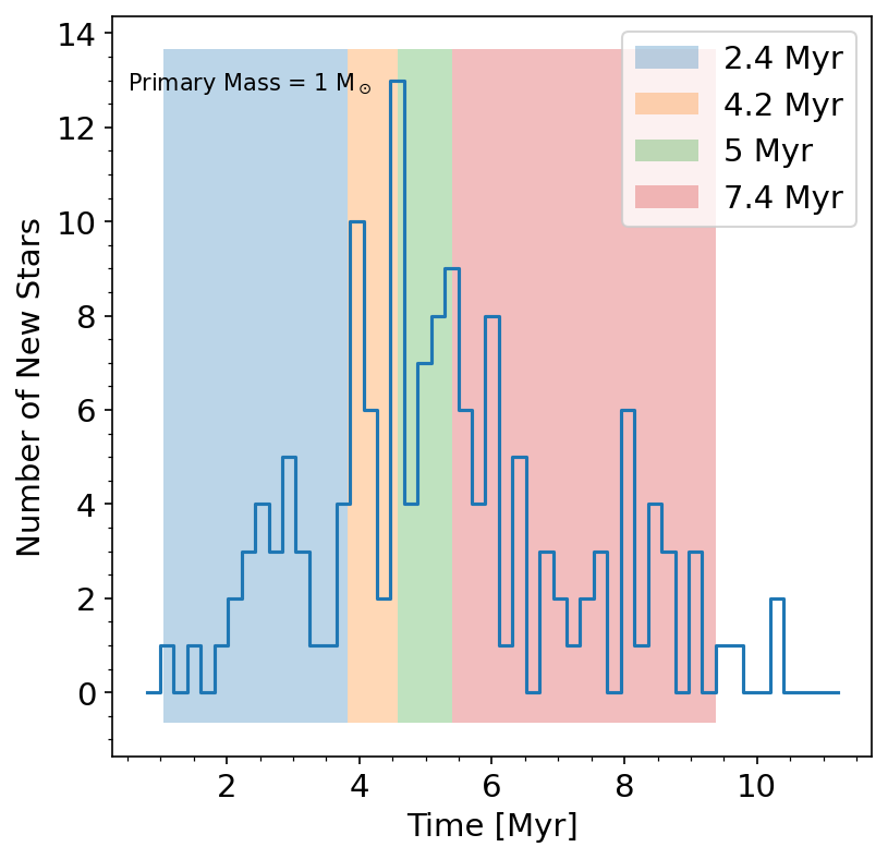
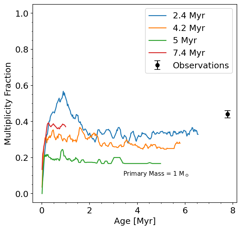
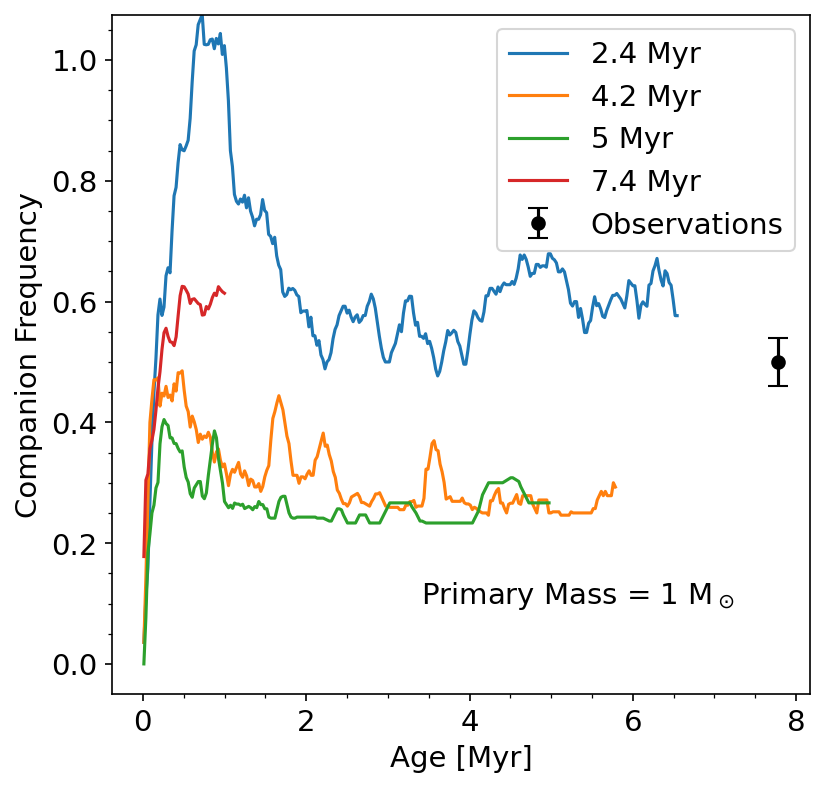
Figure 12: Left: Distribution of formation times for Solar-type stars in the fiducial run. Colored regions show the formation time bins in which the multiplicity properties are calculated in the other panels. Middle & Right: The evolution of $\mathrm{MF}$ and $\mathrm{CF}$ as a function of age for Solar-type stars in various formation time bins. Note that any apparent discrepancy with Figure 11 is due to the different selection criteria since Figure 11 looks at stars that have already stopped accreting. For an analysis of trends see §3 in the main text.

A likely explanation for later forming stars having lower multiplicity is that they form in a different environment. Figure 1 shows that the cloud undergoes global collapse and most star clusters merge to form one massive cluster surrounded by dense gas, until feedback from the stars expel the gas, weakening the gravitational potential well and leading to the expansion of the cluster (Paper II). The first stars form in relative isolation along filaments, while later stars form near existing star clusters. To examine how the “crowdedness” of the birth environment affects multiplicity we define the birth stellar density, which we take to be the stellar mass density around the 32 nearest neighbors of a newly formed star. Figure 13 shows how this initial stellar mass density increases with time and starts to decline after 5 Myr when the cloud begins to disrupt and star formation is quenched in the central cluster (see Figure 1). The remaining gas-free clusters are gravitationally unbound and disperse (Paper II). The other panels of Figure 13 show that both the $\mathrm{MF}$ and $\mathrm{CF}$ for Solar-type stars decline with increasing stellar mass density at formation. This can be attributed to the higher likelihood of dynamical interactions (as there are more stars nearby), allowing for the newly formed star to be either captured by an existing star (increasing the multiplicity of earlier stars relative to later formed ones) or ejected from the gas reservoir.

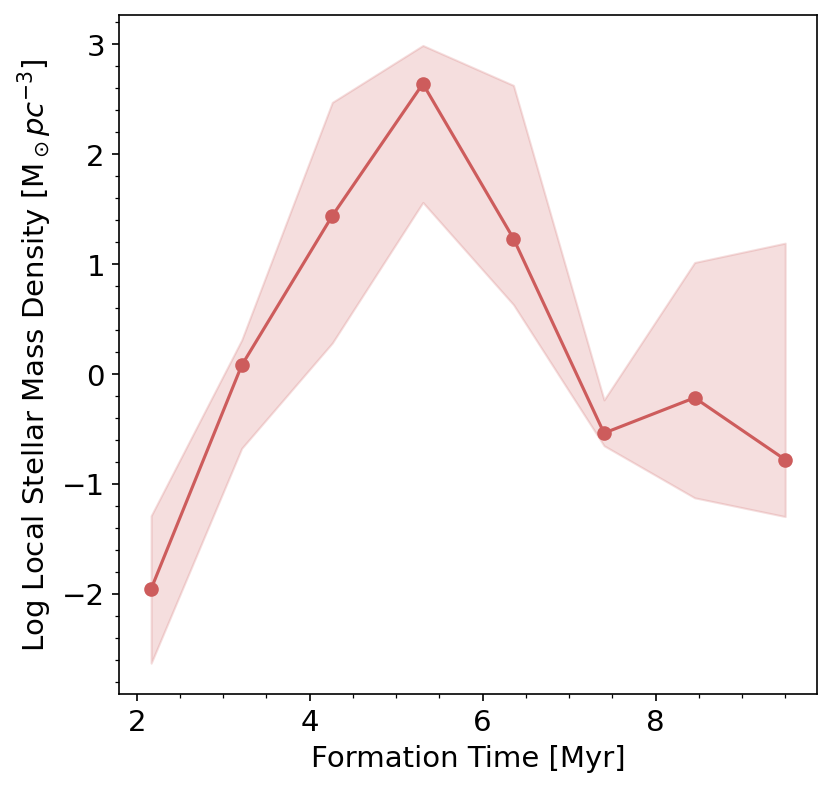
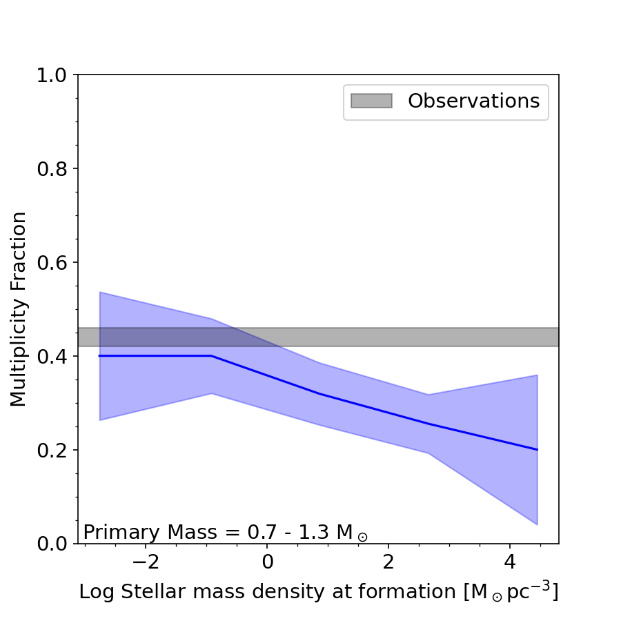
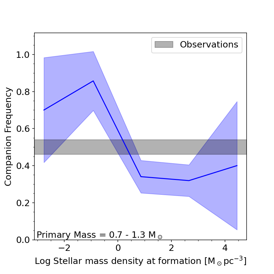
Figure 13: Left: Median stellar mass density around newly formed stars in the fiducial run. The stellar mass density is calculated using the 32 nearest neighbors. Shaded regions show the 25th and 75th percentiles. Middle & Right: Multiplicity fraction and companion frequency in different stellar density bins. Shaded regions show the 1-$\sigma$ sampling uncertainties (see Appendix A for details). The range of observed values for Solar-type field stars from Raghavan et al. (2010) is also shown.

3.3 Multiplicity of YSOs

Figure 14 shows the evolution of the YSO properties in the fiducial simulation. The number of YSOs, which we define to be stars younger than 0.5 Myr, essentially traces the star formation rate. As the cloud disrupts around 6 Myr star formation quenches and the YSO count decreases. To compare with the observations of Tobin et al. (2016, 2022) we calculate the multiplicity fraction of YSOs by taking only systems where all members are YSOs and have a semi-major axis between 20 to $\mathrm{10^{4}}$ AU. We find that the YSO multiplicity in our simulation is comparable to that of Class I protostars in Orion. This is consistent with their expected ages of $\sim 0.1-0.5$Myr (Dunham et al., 2014).

Figure 14: Properties of young stellar objects (YSOs) in the fiducial run, showing the number and multiplicity fraction of YSOs over time. Shaded rectangles show the observed multiplicity values by Tobin et al. (2022) for Class 0 and I protostars in Orion and Perseus, while the transparent blue shaded regions show the 1-$\sigma$ sampling uncertainty of the YSO multiplicity fraction. To make the plot easier to read we apply a 100 kyr rolling average.

4 Effects of initial condition variations on multiplicity

In addition to our fiducial run we carry out a suite of simulations to explore the effects of initial conditions on multiplicity properties. We test for variations in the following initial parameters: the initial cloud surface density, virial parameter, magnetization, metallicity, as well as the interstellar radiation field (ISRF) and turbulent driving; see Table 3 for specifics. These runs use the same turbulent initialization seed. In our analysis we also include two additional runs with the fiducial parameters but with different seeds, which provide a baseline of significance for variations between the runs.

To make the comparisons simpler all values shown in this section are the raw simulation results without corrections to remove short-lived or low-mass ratio companions.

Parameter	Default value	Tested variations	Labels
Initial turbulence	$\alpha_{\mathrm{turb}}=2$ (Marginal boundedness)	x0.5, x2	M2e4_a1, M2e4_a4
Surface density	$\Sigma=63\,\mathrm{M}_{\rm\sun}/\mathrm{pc}^{2}$ (MW average)	x10, x0.1	M2e4_R3, M2e4_R30
Mass-to-flux ratio	$\mu=4.2$ (1% relative magnetic energy)	x0.3, x0.1	M2e4_mu1.3, M2e4_mu0.4
Interstellar Radiation (ISRF)	Solar-circle values (Habing, 1968; Draine, 1978)	x10, x100	M2e4_ISRF10, M2e4_ISRF100
Metallicity	$Z=Z_{\odot}$	x0.1, x0.01	M2e4_Z01, M2e4_Z001

Table 3: List of parameter variations investigated in §4 and the relevant IC labels from Table 1

4.1 Initial level of turbulence

We compare three runs with different levels of turbulence as parameterized by the turbulent virial parameter $\alpha_{\mathrm{turb}}$. The runs all use the same initial turbulent seed, except for the fiducial run ($\alpha_{\mathrm{turb}}=2$), for which we show the results for two additional initial turbulent realizations. The change in velocity dispersion for the different $\alpha_{\mathrm{turb}}$ runs is achieved by scaling the initial velocity fields of the fiducial run (see Table 1). Figure 15 shows that both the multiplicity fraction and companion frequency increases for $M>\mathrm{M}_{\rm\sun}$ stars with increasing turbulence, similar to the results of Cunningham et al. (2018), although the changes are comparable to the variations for different turbulent realizations.

Except for a change in normalization (due to different star formation efficiencies among the clouds) the shape of the semi-major axis distribution is qualitatively similar. We find that increasing the level of turbulence shifts the peak of the misalignment angle distributions toward 90 degrees, similar to the distribution shape resulting from uncorrelated primary and companion spins. This suggests the higher global turbulence reduces the angular momentum correlation on smaller scales.

Increasing the initial turbulence delays star formation, but otherwise the multiplicity fraction of Solar-type stars follows a similar decreasing trend. All runs show decreasing multiplicity with birth stellar density, and the trends agree within 1-$\sigma$ error, but the highest achieved density decreases with the level of turbulence. This means that the increase in multiplicity with stronger turbulence could be explained by the more turbulent clouds having overall lower stellar densities.

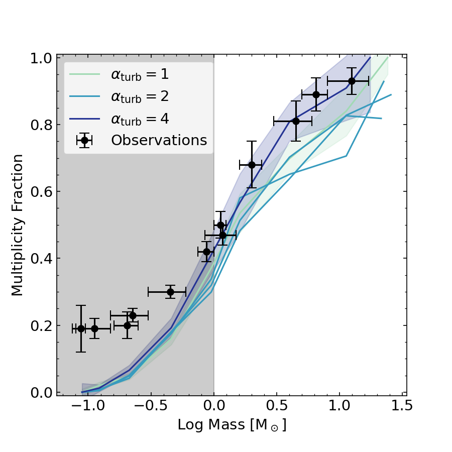
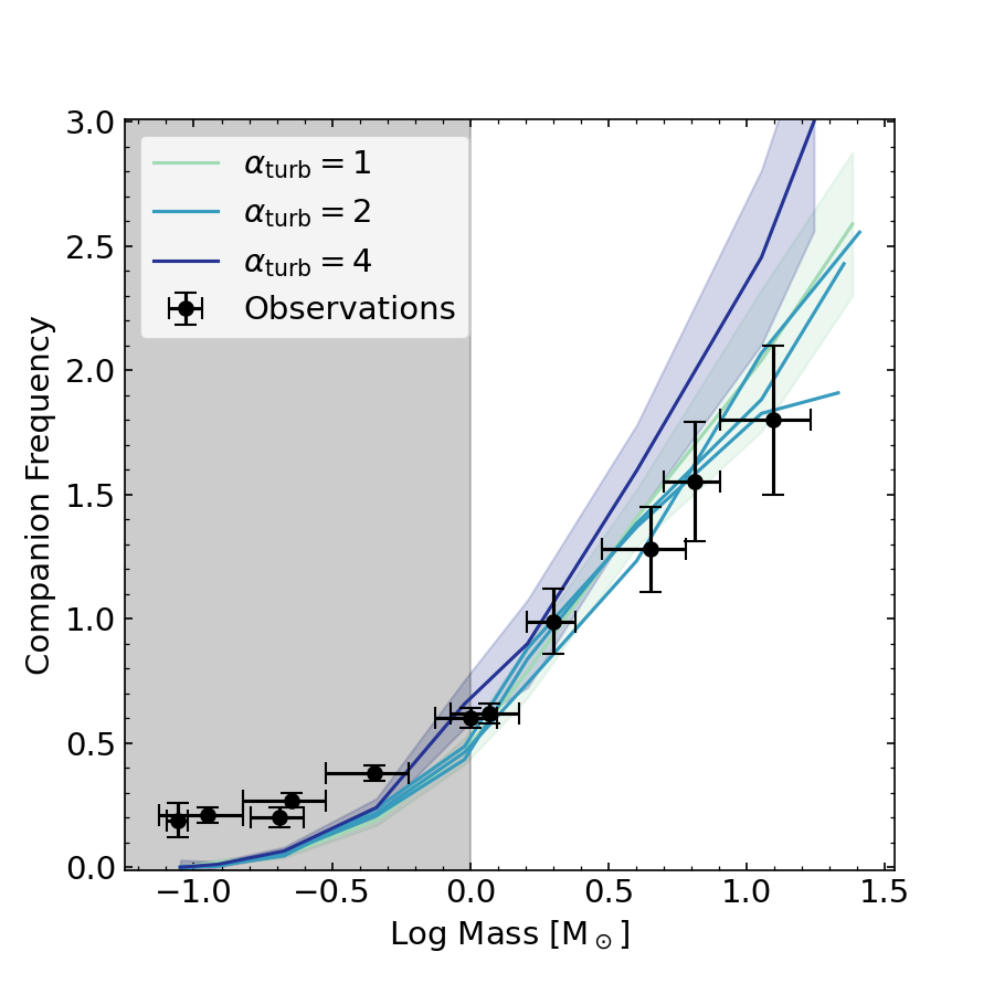
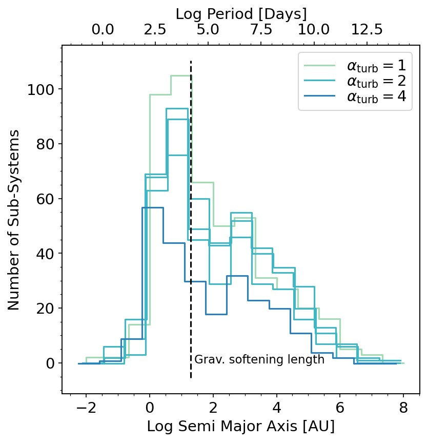
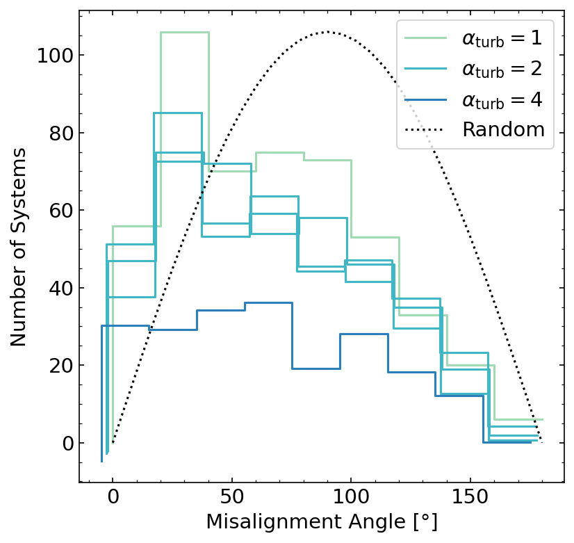
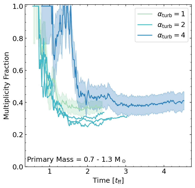
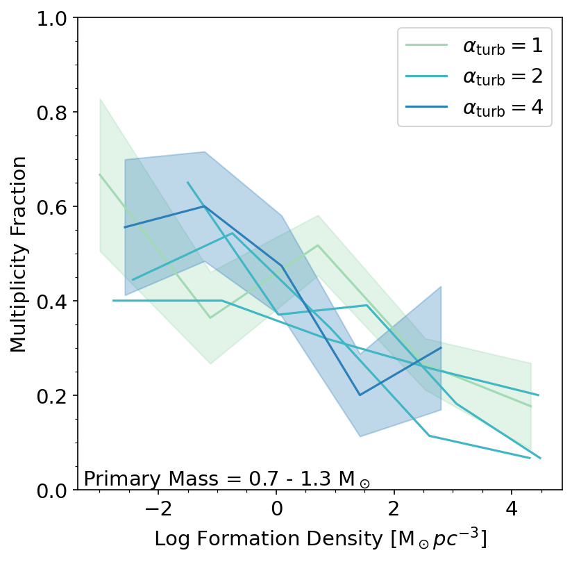
Figure 15: Multiplicity properties for different levels of initial turbulence (M2e4_a1, M2e4, M2e4_a4). The curves do not include corrections for short lived or low-mass ratio companions. For the fiducial M2e4 IC we plot the results from three separate runs that have identical global parameters but different initial turbulent realizations. The top row shows the multiplicity fraction $\mathrm{MF}$ (left), companion frequency $\mathrm{CF}$ (middle), and the distribution of the semi major axis for Solar-type stars (right). For $\mathrm{MF}$ and $\mathrm{CF}$ colored shaded regions show the 1-$\sigma$ sampling errors, which are not plotted for the fiducial M2e4 runs. A grey shaded region shows the mass range potentially affected by the $0.1\,\mathrm{M}_{\rm\sun}$ completeness limit of the simulation. In the semi-major axis distribution the vertical line marks the gravitational softening length of the simulations. The bottom row shows the misalignment angle distribution (left), the evolution of multiplicity for Solar-type stars that are no longer accreting (middle) and the multiplicity fraction for Solar-type stars as a function of birth stellar density (right). The multiplicity time evolution in the middle panel is normalized to the initial cloud freefall time to make comparisons between runs easier. In the left panel a dotted line shows the angle difference distribution resulting from a purely random draw of companion spins. Shaded regions show the 1-$\sigma$ sampling errors, similar to the top row.

4.2 Cloud surface density

Cloud surface density is thought to be a key parameter of star formation (Krumholz & McKee, 2008; Fall et al., 2010; Grudić et al., 2021b) due to its influence on the dynamics of fragmentation and impact on stellar feedback. In addition to our fiducial cloud (M2e4), which has a surface density similar to the MW average ($\Sigma=63\,\mathrm{M}_{\rm\sun}/pc^{2}$) we run clouds with 10 times higher and lower values (M2e4_R3, M2e4_R30). Note that these runs have very different final star formation efficiencies (1%, 9% and 14% in order of increasing surface density). Thus, the low surface density run (M2e4_R30) has about a factor 10 fewer stars than the other runs, making its multiplicity metrics significantly more uncertain.

Figure 16 compares the multiplicity properties across our runs with different initial surface density. We find that increasing surface density leads to lower multiplicity fractions and companion frequencies for higher mass stars as well as a much more pronounced peak in the semi-major axis distribution near the gravitational softening length ($\sim 20\,\mathrm{AU}$). Increasing the initial cloud surface density does not affect the spin alignment between primaries and their companions (bottom left panel of 16), however the low surface density run shows an essentially flat distribution. As in all previously discussed runs, the multiplicity fraction of Solar-type stars decreases with time, which can be explained by the increasing stellar density around newly forming stars. We find that the relationship between the birth stellar density and the multiplicity fraction is similar between the runs, and their cut-off value increases with initial surface density. This also provides an explanation as to why both $\mathrm{MF}$ and $\mathrm{CF}$ decrease with increasing surface density: the denser the cloud, the higher the stellar density, leading to more dynamical interactions and thus lower multiplicity at the end of the simulations.

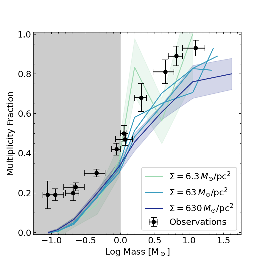
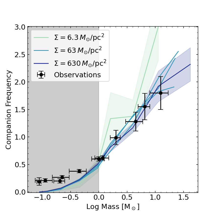
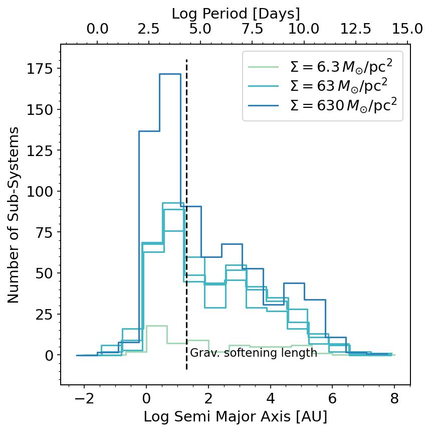
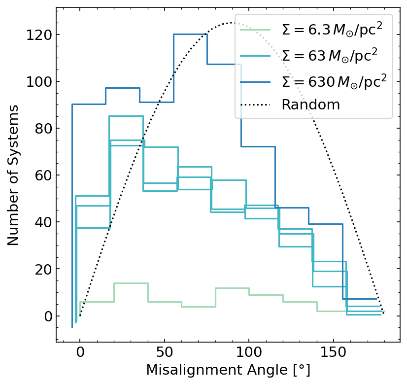
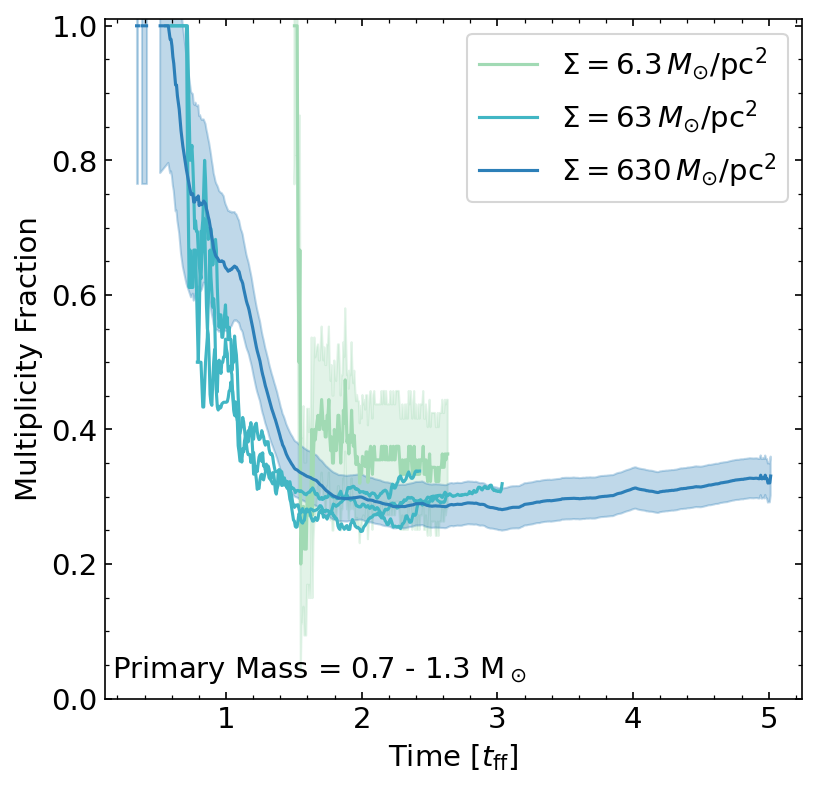
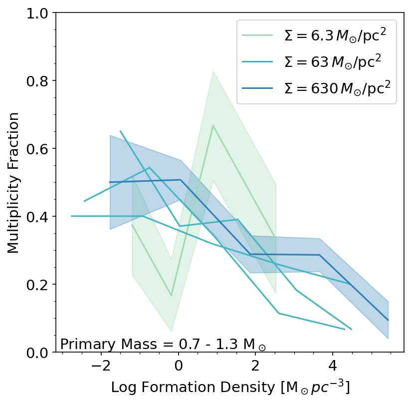
Figure 16: Same as Figure 15 but for different initial cloud surface densities (M2e4_R3, M2e4, M2e4_R30).

4.3 Cloud magnetization

Star formation efficiency is sensitive to the cloud mean magnetic field (e.g., Padoan et al., 2012), with efficiency decreasing with stronger fields (Paper III). This result suggests multiplicity might also depend on the magnetic field. In this section we present runs for clouds with increasing initial magnetic fields, corresponding to initial normalized mass-to-flux ratios $\mu$ of 4.2, 1.3 and 0.4 (M2e4, M2e4_mu1.3, M2e4_mu0.4, see Table 1).

Figure 17 shows that the strong field cloud has a significantly higher multiplicity fraction for Solar-type stars, an effect proposed by prior work (Lee et al., 2019). However, there is essentially no change difference between the fiducial, weak ($\mu=4.2$) and intermediate ($\mu=1.3$) field runs. For all three cases there are no significant variations in either the semi-major axis distribution or the distribution of the misalignment angle. The increased magnetic fields provide significant support to the cloud against collapse, which delays star formation. Apart from this delay the multiplicity fraction of Solar-type stars follows a similar declining trend with time. The weak and intermediate field runs provide a similar relationship between the birth stellar density and the multiplicity fraction, while the highly magnetized run has significantly higher multiplicities at similar stellar densities. In Guszejnov et al. (2020) we show that regardless of the initial magnetic field strength, the magnetic energy density at high densities follow the same trend ($v_{\mathrm{Alfv\'{e}n}}\sim c_{s}$), due to the turbulent magnetic dynamo. This means that the effects of the global initial magnetic field do not propagate to densities higher than $\rho_{B}>B_{0}^{2}/(\mu_{0}c_{s})$, where $B_{0}$, $c_{s}$ and $\mu_{0}$ are the initial magnetic field strength, the sound speed and the vacuum permeability respectively. So the initial magnetic field only influences multiplicity properties if $\rho_{B}$ is comparable to the densities of star forming cores.

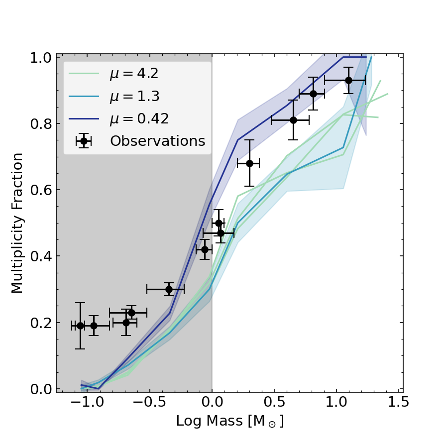
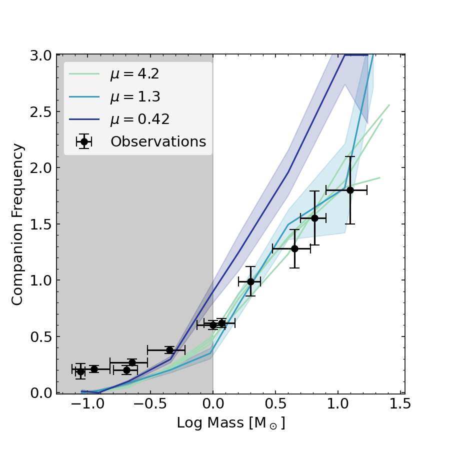
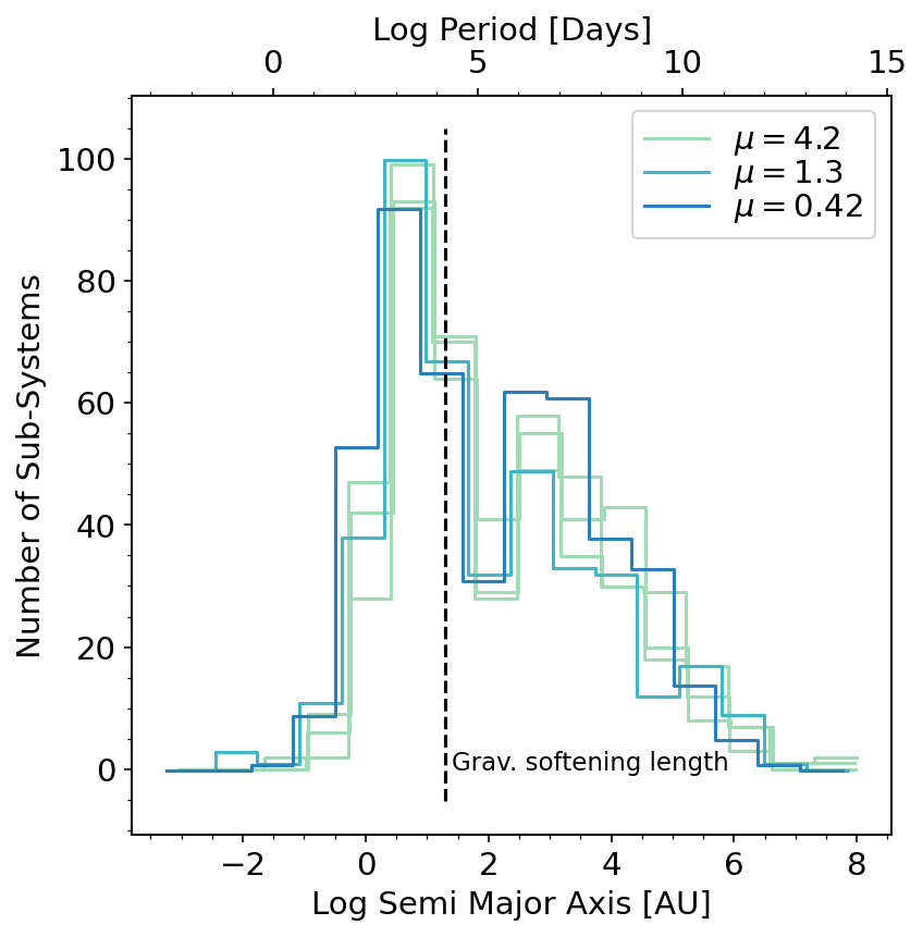
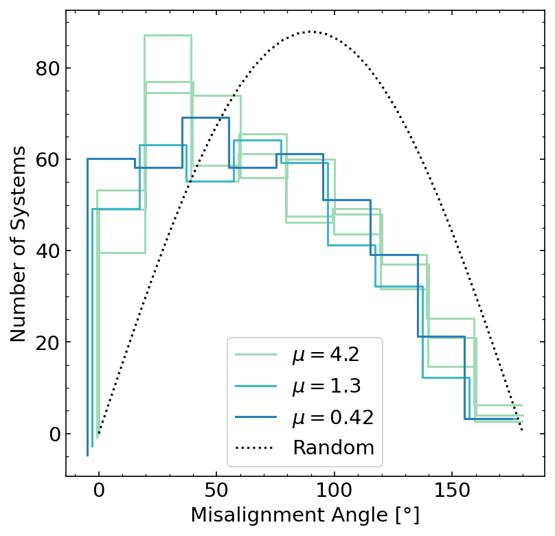
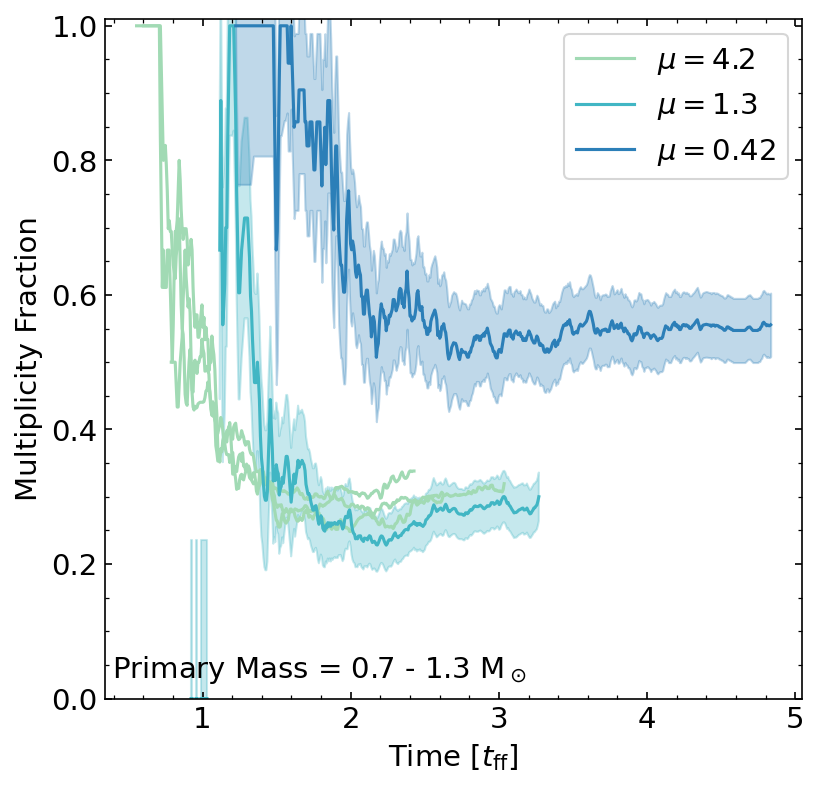
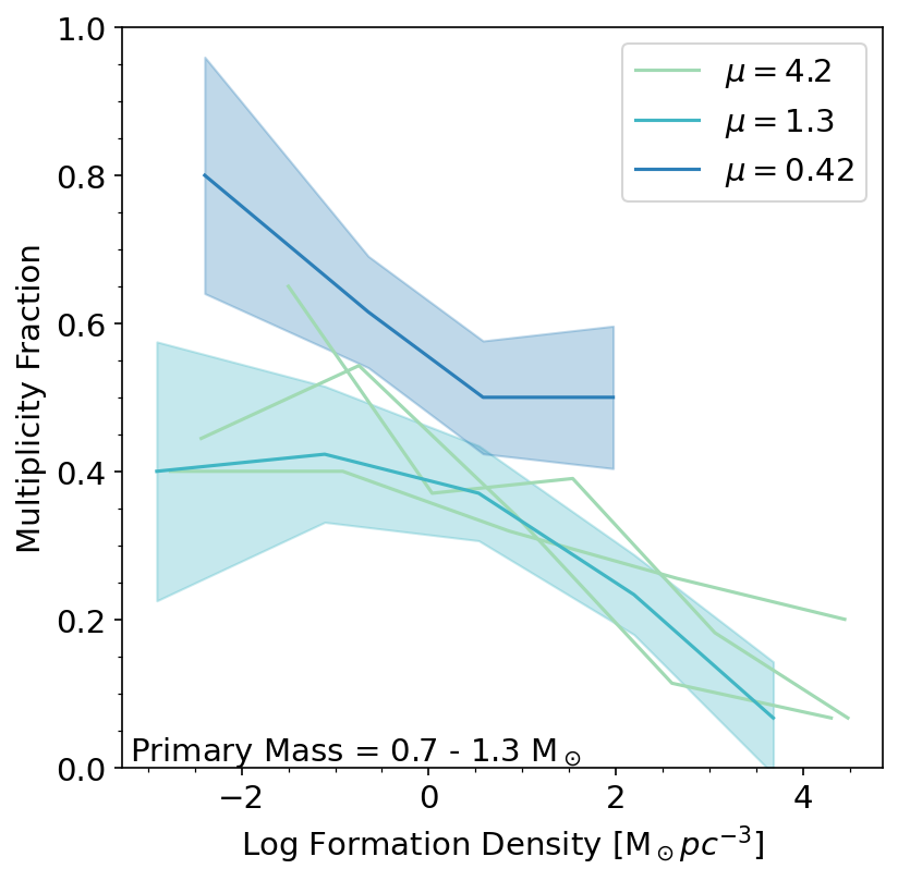
Figure 17: Same as Figure 15 but for different levels of initial magnetization (M2e4, M2e4_mu1.3, M2e4_mu0.4).

4.4 Cloud metallicity

Metallicity is a key property of interstellar gas, which directly sets its thermodynamic behavior, so it is expected to have a major impact on star formation (Krumholz, 2014). In this section we present three runs with decreasing initial gas metallicities, corresponding to Solar, 10% of Solar and 1% of Solar values (M2e4,M2e4_Z01 and M2e4_Z001 respectively, see Table 1).

We find that metallicity significantly affects the star formation process, notably it shifts the IMF to significantly higher masses (see Paper III for details). However, Figure 18 shows that varying the metallicity of the gas has no clear effect on either the multiplicity fraction or the companion frequency, similar to the results of Bate (2019). While the normalization of the semi-major axis distribution is affected by the differences in the overall star formation efficiency, its shape appears to be similar between the three runs. Decreasing the metallicity mildly flattens the the misalignment angle distribution, i.e., makes anti-parallel companions slightly more likely. The evolution of the multiplicity fraction for Solar-type stars declines similarly for the fiducial and the 10% Solar metallicity runs, but for the 1% run we find significantly lower multiplicities and an increasing trend instead of a decreasing one. The relationship between the multiplicity fraction and the birth stellar density is also different between the runs; in the low metallicity clouds there is no clear relationship between the two quantities.

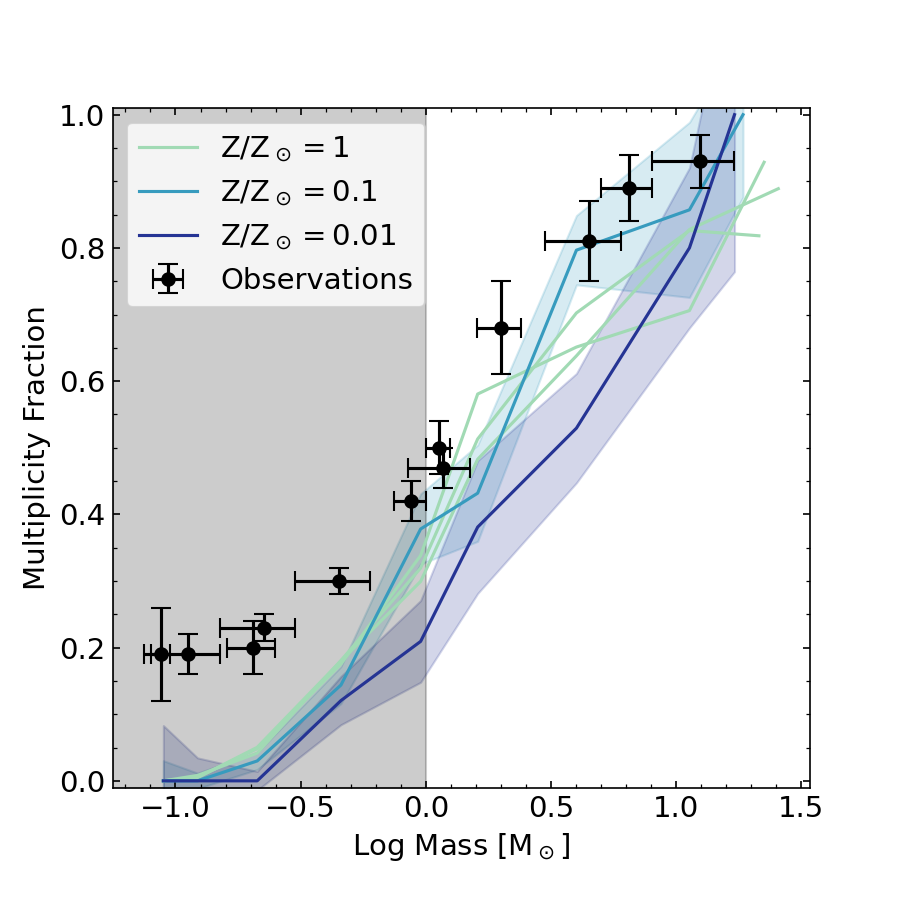
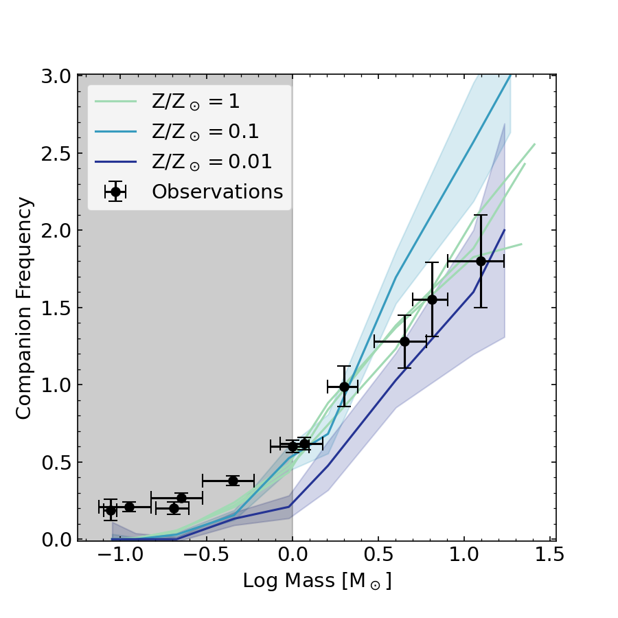
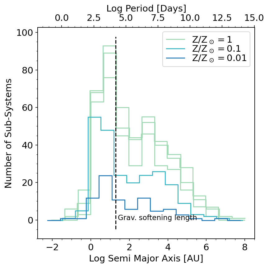
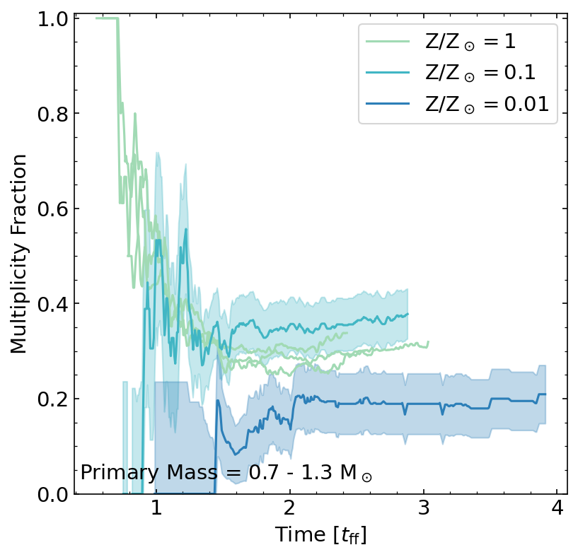
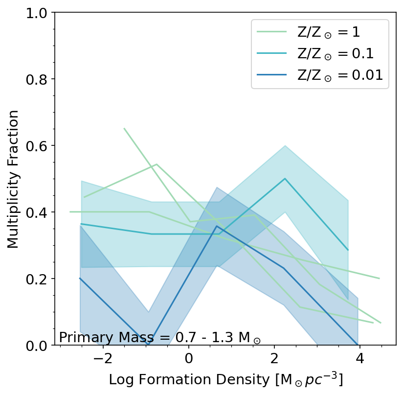
Figure 18: Same as Figure 15 but for different levels of initial gas metallicity (M2e4, M2e4_Z01, M2e4_Z001).

4.5 Interstellar Radiation Field

The interstellar radiation field (ISRF) is set by the radiation of previously formed stars in the local galactic environment. The ISRF varies as a function of the galactocentric radius, so clouds located closer to the galactic center experience higher ISRFs. Thus, the radiative environment is expected to vary significantly between star-forming regions. We compare the multiplicity properties in three runs with progressively higher background radiation fields, starting from our fiducial run, which adopts the Solar-circle value of 1 Draine (M2e4), followed by runs with 10 times (M2e4_ISRF10) and 100 times (M2e4_ISRF100) higher radiation energy densities, see Table 1.

We find that increasing the ISRF increases the gas temperature and shifts the IMF to mildly higher masses (see Paper III for details). However, figure 19 shows a mild increase in both the multiplicity fraction and the companion frequency at high masses. The increased ISRF has little effect on the semi-major axis or the misalignment angle distributions. Similar to the case of metallicity variations, the mildly increased ISRF run shows similar $\mathrm{MF}$ evolution for Solar-type stars while M2e4_ISRF100 shows a qualitatively different evolution where $\mathrm{MF}$ increases with time. Nevertheless, the three simulations show a similar relationship between the stellar densities at formation and $\mathrm{MF}$, although the $\mathrm{MF}$ is consistently lower for M2e4_ISRF100. Note that this is also the run with the most shift in the IMF towards higher masses, which likely affects the comparisons of Solar-type stars.

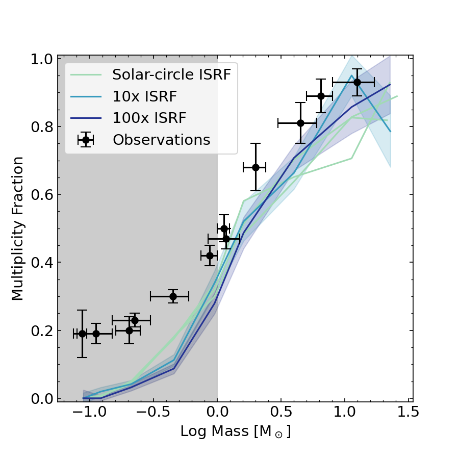
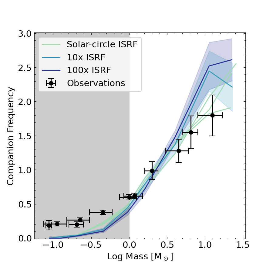
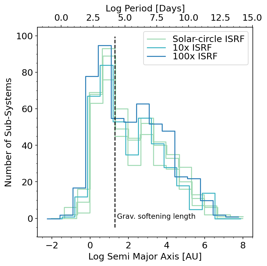
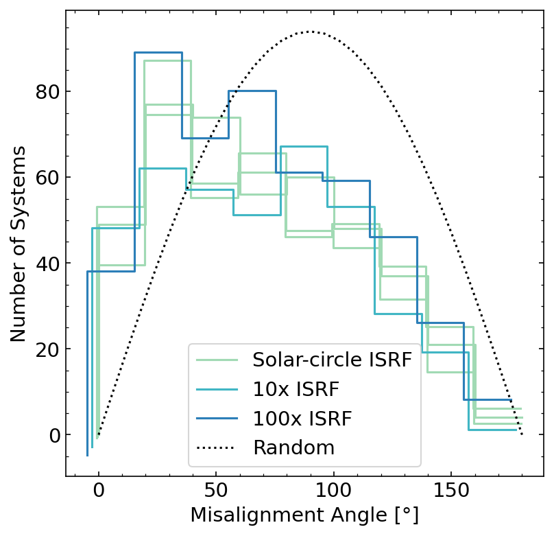
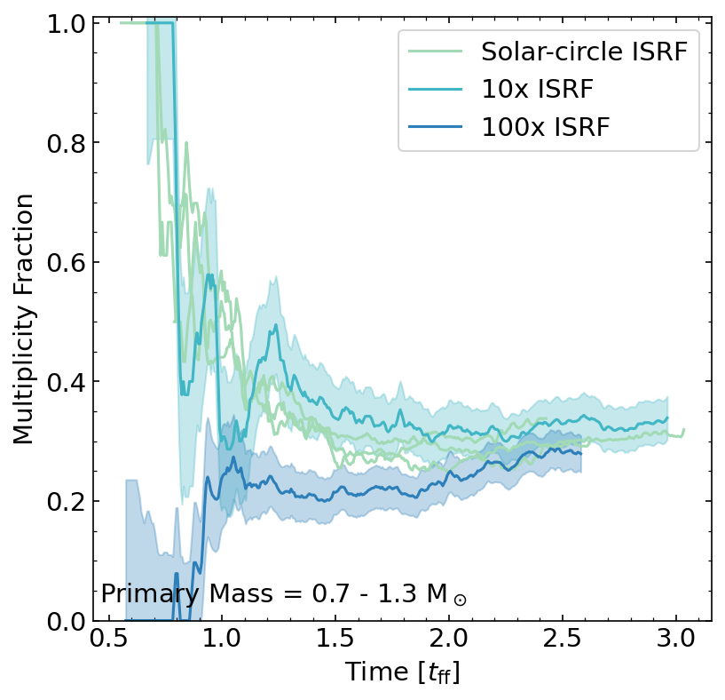
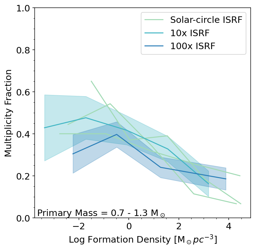
Figure 19: Same as Figure 15 but for different levels of interstellar radiation field (M2e4, M2e4_ISRF10, M2e4_ISRF100).

4.6 Cloud setup and turbulent driving (Box vs. Sphere)

We note in §2.1.2 that there are several common assumptions in the literature for the geometry and boundary conditions of simulated star forming clouds. In this subsection we compare the results of a periodic Box configuration relative to our fiducial Sphere run. The Box runs differ from the fiducial run in two important aspects. First, periodic boundary conditions lead to both an order-of-magnitude shallower gravitational potential (Federrath & Klessen, 2012) and prevent the escape of radiation and gas. Second, the Box setup starts from a self-consistent, pre-stirred state, and this external driving continues throughout the run, providing energy for turbulent modes on the box scale that cascade down to smaller scales. To disentangle the effects of these two factors, we compare three M2e4 runs (Table 1): 1) our fiducial Sphere run, 2) a Box run with continuous external driving and 3) a Box run where we turn off the driving after the initial “stirring” phase.

We find that the periodic boundary conditions have little effect on multiplicity properties when comparing the “Sphere” and “Box, decaying” runs, whose results agree within 1-$\sigma$ uncertainty for $\mathrm{MF}$, $\mathrm{CF}$, the semi-major axis and the misalignment angle distributions (see Figure 20). There is a difference in the length of the initial transient in the evolution of the multiplicity fraction of Solar-type stars. This delay is likely due to the stronger initial turbulent support in the Box run, since the periodic boundary conditions weaken the gravitational potential. As turbulence decays the “Box, decaying” run starts following the same trend as the fiducial Sphere run.

Turbulent driving, however, has a significant effect on the multiplicity fraction and companion frequency, leading to significantly higher values for both $\mathrm{MF}$ and $\mathrm{CF}$ on all mass scales. This is the only run in our parameter study that shows a change in sub-solar multiplicities. We attribute this difference to the turbulent driving, which weakens gravitational focusing and leads to lower stellar densities in star-forming regions. In other words, star formation is more distributed, which reduces the frequency of dynamical interactions thus leading to higher multiplicities on all mass scales.

We find that all three runs exhibit a similar relationship between the birth stellar density and the multiplicity fraction, but the Box run with turbulent driving has a lower maximum density, consistent with the higher multiplicity values we find for that run.

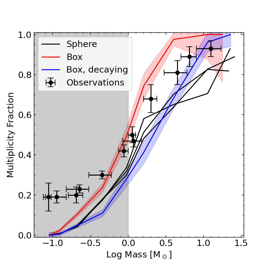
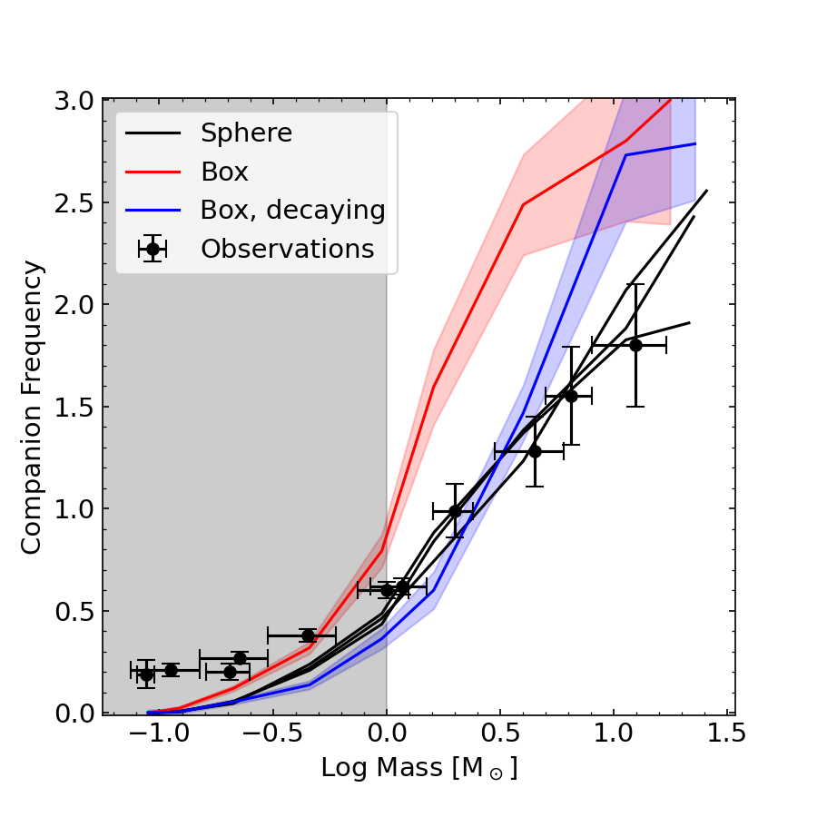
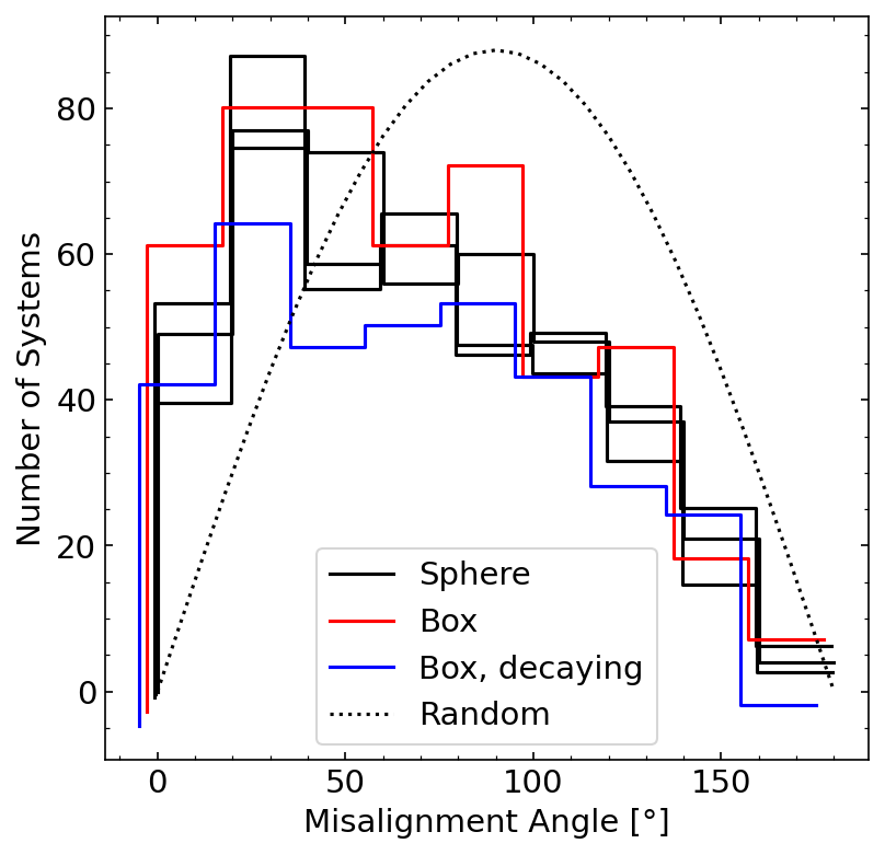
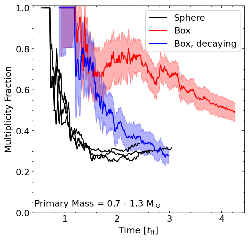
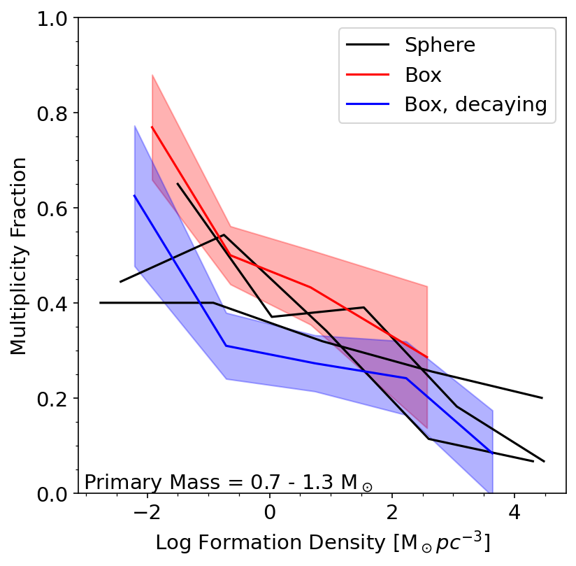
Figure 20: Same as Figure 15 for runs using fiducial M2e4 parameters but with different initial and boundary conditions (“Sphere”, “Box”, “Box, decaying”).

5 Discussion

5.1 Multiplicity in the fiducial simulated cloud

Similar to previous simulations in the literature (i.e., Bate, 2009b, 2012; Krumholz et al., 2012; Mathew & Federrath, 2021) our simulations reproduce the rising trend with mass in both the multiplicity fraction and companion frequency. We find that the simulations match recent observations (Offner et al., 2022) at all but the lowest mass scales (Figure 21). The discrepancy at low masses can be explained by our choice of ignoring all brown dwarfs during the identification of multiples, motivated by the completeness limit of the simulation being at $\sim 0.1\,\mathrm{M}_{\rm\sun}$.

We find that the multiplicity properties of stars depend on their formation time, i.e., early forming stars tend to have more companions than those that form near the end of the star formation process (Figure 12). We find that the primary cause of this decrease is not stars losing companions, i.e., through dynamical interactions (Heggie, 1975), but that later forming stars are born with fewer companions. We show that there is a correlation between multiplicity (i.e., $\mathrm{MF}$ and $\mathrm{CF}$) and the birth stellar density. This allows us to explain the decreasing trend with formation time, as locally collapsing regions merge and form a dominant, central, gas rich cluster, in which stars form at much higher stellar densities than in the early phase ($<4\,\mathrm{Myr}$) of cloud evolution when they formed along filaments (Figure 1). In this dense stellar environment dynamical interactions with other stars are much more likely, leading to newly formed stars being captured by existing ones, as well as companions being ejected.

Similar numerical works in the literature mostly report only these “raw” values (e.g., Bate, 2012, 2019; Mathew & Federrath, 2021) without correcting for observational completeness limits and chance alignments that the algorithm mistakenly identifies as a multiple star system. In this work we apply two simple corrections to account for these effects: we ignore companions with mass ratios below most observational completeness limits ($q<0.1$) and those that are not bound to their companion for at least 100 kyr and two full orbits. We find that the combined effects of these corrections dramatically reduces the number of companions for $>1\,\mathrm{M}_{\rm\sun}$ stars and consequently lower $\mathrm{MF}$ above a few $\mathrm{M}_{\rm\sun}$ (as these stars tend to have lower $q$ companions). Overall this means that our simulations under-predict both the $\mathrm{MF}$ and $\mathrm{CF}$ compared to observations. One possible explanation for this discrepancy is that stars in our simulations lose companions due to the inaccurate short-range gravitational forces in the simulation (i.e., having finite gravitational softening). We find this explanation to be unlikely as we find a pile-up of companions at the gravitational softening length (Figures 5-7), the net effect of the gravitational softening is likely to increase the number of companions by trapping them at that length scale and preventing violent, short-range N-body interactions that could eject companions. A more likely explanation is the apparent lack of stable protostellar disks in the simulations. This means that from three main pathways of binary formation (core fragmentation, disk fragmentation and capture, see Tohline 2002; Kouwenhoven et al. 2010) our simulation is missing disk fragmentation, which could conceivably make up for the missing companions relative to observations (Kratter & Lodato, 2016). Furthermore, the presence of protostellar disks would push companions mass ratios towards unity (see e.g., Kratter et al., 2010; Farris et al., 2014; Duffell et al., 2020). In addition, removal of angular momentum by magnetic breaking tends to drive accretion onto the more massive primary (Zhao & Li, 2013), thereby decreasing the mass ratio. Thus, the influence of disks and inclusion of non-ideal MHD together would likely shift currently small mass ratios above the $q=0.1$ limit, significantly increasing $\mathrm{MF}$ and $\mathrm{CF}$ at the high mass end after correcting for observational incompleteness (i.e., the difference between the “raw” and “corrected” results in Figure 3 would be smaller). Finally, it is possible that our choice of initial conditions (i.e., geometry and turbulent driving) is the main cause of the discrepancy (see §5.2). This explanation is further supported by the fact that we find good agreement between the Box run and the semi-analytic core fragmentation model of Guszejnov et al. (2017), which follows only core fragmentation and has similar initial and boundary conditions (see Figure 21). Note that Guszejnov et al. (2017) ignores dynamical interactions, which is likely the explanation for the slightly higher multiplicity values it predicts relative to the Box run. After correcting for observational biases the Box results agree well with the observed $\mathrm{MF}$ and $\mathrm{CF}$ for $M>\mathrm{M}_{\rm\sun}$ stars, which is also the mass range unaffected by the $0.1\,\mathrm{M}_{\rm\sun}$ completeness limit of the simulation.

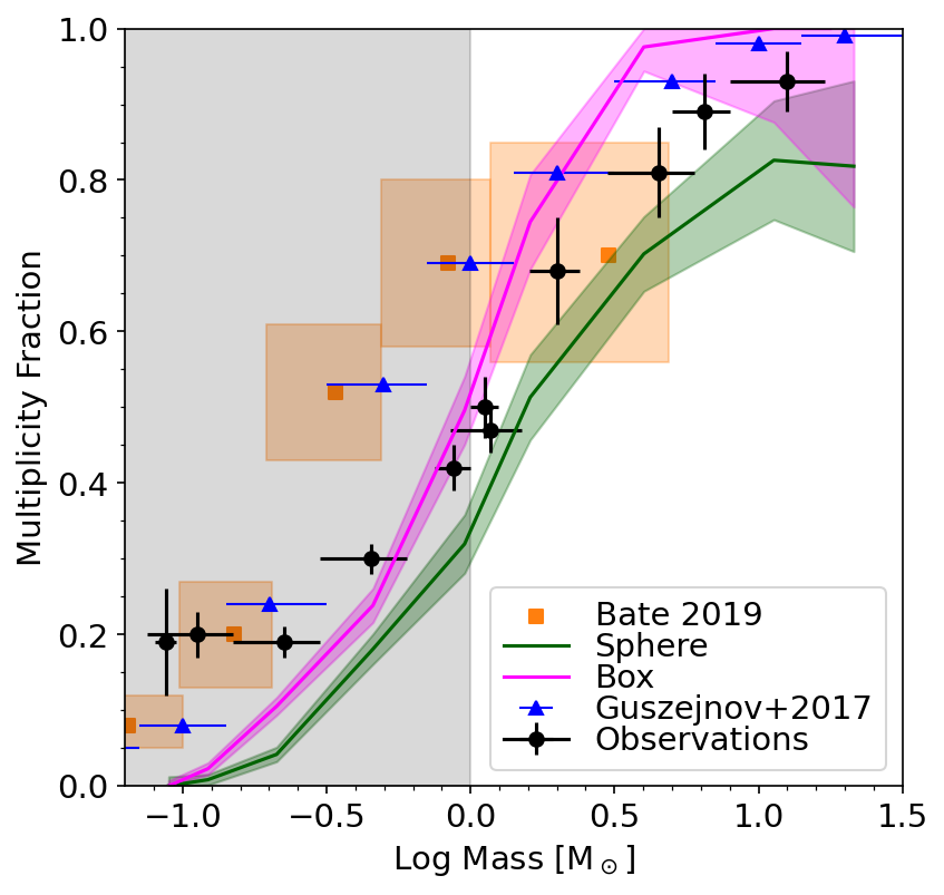
Figure 21: Left: Multiplicity fraction as a function of primary mass in this work (both Sphere and driven Box runs, without corrections), in RHD simulations from Bate (2019), in semi-analytical predictions from Guszejnov et al. (2017) and in observations (Offner et al., 2022). 1-$\sigma$ uncertainties are shown with either colored shaded regions or errorbars, while a grey shaded region shows the mass range potentially affected by the $0.1\,\mathrm{M}_{\rm\sun}$ completeness limit of the simulation. For high mass stars the Box results agree well with the semi-analytical core fragmentation model of Guszejnov et al. (2017) and the RHD simulations of Bate (2019), while observations fall between the values in the Sphere and Box runs. Middle & Right: Multiplicity fraction and companion frequency values for the driven Box run, using a similar notation as Figure 3. Unlike the Sphere run shown in Figure 3, the Box run results after corrections agree well with observations for both $\mathrm{MF}$ and $\mathrm{CF}$ (for stars with masses above $\mathrm{M}_{\rm\sun}$). Discrepancies at lower masses are likely due to the $0.1\,\mathrm{M}_{\rm\sun}$ completeness limit of the simulation.

For all primary masses we find that the mass ratio distribution in the fiducial run is consistent with randomly drawing companions from the initial mass function of the simulation (Figure 4). For Solar-type stars, correcting for chance alignments leads to lower values at lower mass ratios ($q<0.2$). Observations find the q-distribution of Solar-type stars is flat (Raghavan et al., 2010) with an slight peak at $q\approx 1$ (see MDS17). This uniform distribution is inconsistent with randomly drawing from the observed MW IMF, but it should be noted that the discrepancy is only significant at $q\approx 0.2$. Note that these observations are incomplete in this mass ratio range for short-period binaries, i.e., for companions with periods $\mathrm{Log}P/\mathrm{day}<4.5$ the observations are only complete for $q>0.5$ (see Figure 28 in MDS17). After applying this correction to our results, we find a flatter distribution with a marginal peak around $q\approx 0.2$. This peak is dominated by low-$q$ companions at the softening length from their primary, so its significance strongly depends on the applied observational completeness limit. Similarly, we find that the agreement between the simulation and observations improves for both the semi-major axis and the eccentricity distributions after all corrections are applied. However, applying this correction significantly reduces the $\mathrm{MF}$ and $\mathrm{CF}$ for Solar-type stars, increasing the discrepancy with observations. It should be noted that the aforementioned “pile-up” of companions at the gravitational softening length ($\sim 20\,\mathrm{AU}$) plays an out-sized role in this dramatic change (see Figure 5). As previously noted we are unable to correct this pile-up as companions could spiral into shorter periods, be ejected or relax to longer orbits. Correcting for the observational bias for Solar-type stars (based on MDS17) removes these companions, which implicitly assume that they either migrate to smaller scales or are ejected from the system. Furthermore, observations find a significant fraction of binaries have near-equal mass (twin) companions, which are missing in our simulations. This is likely due to the lack of long-lived protostellar disks, as disk fragmentation is more likely to produce near-equal mass companions (Kratter et al., 2010), as disks allow companions to “steal” mass from the primary star. Disk accretion would also cause mass to be more equally distributed for secondaries that formed from turbulent fragmentation and migrated into or to close proximity of the primary’s disk (Duffell et al., 2020).

We track the angular momentum accreted by stars in the simulation and use its direction as a proxy for the direction of the spin of the star, as stars (i.e., sink particles) in the simulation can not lose angular momentum. Protostars are thought to inherit the angular momentum of their natal core, which would naturally lead to most binaries having similar spin alignments. Observations have found multiple protobinary systems where the protostellar outflows are misaligned (Lee et al., 2016). We find that the distribution of the misalignment angle (i.e., angle between spins of the primary and its companions) is peaked towards lower values, i.e., companions tend to be aligned with their host stars (see Figure 9), exhibiting a less random distribution than prior results Offner et al. (2016); Lee et al. (2019). The distribution is fairly wide, and there is a significant number of companions with anti-parallel spin alignments. We find that the companions of more massive stars tend to be less aligned than companions of lower mass stars and that spin alignment increases over time. Figure 7 shows that massive stars are slightly more likely to have companions that formed at large distances ($\sim 10^{5}\,\mathrm{AU}\sim 1\,\mathrm{pc}$), making their spin directions more likely to be unrelated. Also, high-mass stars accrete from a significantly larger gas reservoir over a longer accretion time period rather than a more localized gas “core" (Paper I), and thus are less likely to have companions with aligned angular momentum vectors. Such misalignment has been found in recent observations of massive protostars (Avison et al., 2021). While multiple systems formed via turbulent fragmentation are less likely to have aligned spins compared to those formed by disk fragmentation (Offner et al., 2016; Lee et al., 2019), systems that accrete from the same limited gas reservoir apparently still exhibit some spin correlation.

5.2 Connecting cloud properties and multiplicity

We analyze a suite of simulations where the initial properties of the cloud are varied (Table 3) and find that most multiplicity properties are insensitive to global cloud parameters. We find that multiplicity properties (i.e., $\mathrm{MF}$, $\mathrm{CF}$) can significantly vary between runs with identical global parameters but different turbulent realizations (see §4), making it challenging to identify weaker trends. Note that observations are only able to constrain variations to changes in metallicity, as other properties of the natal cloud are not readily available once star formation ends. Moe et al. (2019) showed that the multiplicity of Solar-type stars decreases with metallicity, due to a relative lack of close binaries.

These trends are summarized in Table 4, note that the changes in the final star formation efficiency (SFE) and the shape of the IMF are investigated in detail in Paper III, here we just state the results. Similar to Bate (2019) we find that the initial cloud metallicity has no clear effect on multiplicity values, even though observations show a strong anti-correlation (Moe et al., 2019). A possible explanation is that other cloud parameters (e.g., surface density) co-vary with metallicity for the observed multiples. Note that this trend was shown for close binaries only, which our simulation under-predict due to the lack of disk formation, which could also explain the discrepancy. We find that in most runs changes in the multiplicity fraction and companion frequency coincide with an opposite change in the stellar mass density around newly formed stars. This provides a potential explanation of these trends as an increasing stellar density means a higher chance for dynamical interactions, disrupting existing binaries and making it harder for newly formed stars to capture a companion. In our simulations an increase in the initial turbulence or continuous driving both weaken gravitational focusing in the cloud, leading to lower stellar densities. Starting from lower initial gas densities has a trivially similar effect. Overall, we find that multiplicity properties are sensitive to a different set of initial conditions than the IMF (see Paper III).

We note that changing the initial surface density dramatically affected the fraction of companions at or below the gravitational softening length, implying that the surface density of the natal cloud likely influences the period distribution. Although we find no monotonic trend in either $\mathrm{MF}$ or $\mathrm{CF}$ with increasing initial magnetic field strength, we note that the run with the strongest field produces significantly higher multiplicity values, similar to the results of Lee et al. (2019).

The spins of companions in all our simulations are more aligned than random pairings with their primaries, however several initial parameters affect this distribution. Increased initial turbulence and reduced surface density both lead to more randomized spin alignments. The effects of surface density and turbulence can be potentially explained by the changes in how distributed star formation is within the cloud. Higher surface density or weaker turbulent support enhance the gravitational focusing of the parent cloud, leading to the formation of more massive and denser clusters (Guszejnov et al., 2022a). In a denser environment dynamical interactions are more common, so stars are more likely to both lose their original companions and capture new ones. Lowering the metallicity also leads to an increase in the randomness of spin alignment. This trend can potentially be explained by low $Z$ leading to higher gas temperatures, which makes protostellar cores larger, which leads (on average) to increased initial separation between companions that form through core fragmentation, making alignment less likely.

Parameter	Final SFE	IMF change	Stellar density	Effect on multiplicity properties
Initial turbulence ($\alpha_{\mathrm{turb}}\uparrow$)	$\downarrow$	Negligible	$\downarrow$	$\mathrm{MF}\uparrow$, $\mathrm{CF}\uparrow$; spins more likely to be random
Surface density ($\Sigma\uparrow$)	$\uparrow$	Negligible	$\uparrow$	$\mathrm{MF}\downarrow$, $\mathrm{CF}\downarrow$; more companions at softening length
Mass-to-flux ratio ($\mu\downarrow$)	$\downarrow$	Steeper slope	$\downarrow$	$\mathrm{MF}\uparrow$, $\mathrm{CF}\uparrow$; variations only present in $\mu=0.42$ run
Metallicity ($Z\downarrow$)	$\downarrow$	mild $\rightarrow$ shift	No trend	$\mathrm{MF}$, $\mathrm{CF}$ no longer correlated with stellar density; spins more likely to be random
Interstellar Radiation (ISRF$\uparrow$)	mild $\uparrow$	mild $\rightarrow$ shift	$\uparrow$	Mild $\mathrm{MF}\uparrow$, $\mathrm{CF}\uparrow$ at high masses
Geometry (Box vs Sphere)	N/A	Negligible	No trend	Mild $\mathrm{MF}\uparrow$, $\mathrm{CF}\uparrow$ at high masses
Turbulent driving	N/A	Steeper slope	$\downarrow$	$\mathrm{MF}\uparrow$, $\mathrm{CF}\uparrow$ for all masses

Table 4: Summary of results from §4, showing the trends in the final star formation efficiency, the shape of the IMF, the average at formation stellar density and a general description on how multiplicity properties are affected (see Figures 15-20 for details). Note that in case of the Box geometry there is no final SFE as the simulation is terminated when the periodic box is filled with an unphysical level of radiation.

5.3 Caveats

While the simulation presented here are the current state-of-the-art for simulating star-forming clouds, like other simulations in the literature STARFORGE employs a large number of significant approximations and assumptions to make the simulations computationally tractable (see the Methods Paper for detailed discussions).

In particular, the runs used here have a $\sim 30\,\mathrm{AU}$ Jeans-resolution, i.e. fragmentation on scales smaller than this are not resolved. This has dramatic effects on the formation of protostellar disks, causing the simulation to potentially miss close binaries that formed from disk fragmentation and overestimate stellar masses. Furthermore, the simulations have a $\sim 20\,\mathrm{AU}$ gravitational softening length that creates a “pile-up” of companions at this scale in the semi-major axis/period distribution (see Figure 5).

The simulations treat MHD in the ideal limit, assuming perfect coupling between the neutral gas and the magnetic fields. This approximation becomes invalid on the scale of protostellar disks, preventing the formation of long lived protostellar disks and the formation of binaries through disk fragmentation. Also, we show that the initial and boundary conditions of the cloud can affect multiplicity properties, so for a more predictive simulation a self-consistent connection to larger scales is required.

6 Conclusions

In this work we analyze the stellar multiplicity properties in the STARFORGE radiation-magnetohydrodynamic simulations. These simulations follow the evolution of mid-sized molecular clouds ($M=20000\,\mathrm{M}_{\rm\sun}$) taking into account gravity, gas thermodynamics, turbulence, magnetic fields, and radiation as well as stellar feedback processes (jets, radiation, winds, SNe). The simulation suite consists of our fiducial cloud with MW average properties ($\Sigma=63\,\mathrm{M}_{\rm\sun}/\mathrm{pc}^{2}$, $\alpha_{\mathrm{turb}}=2$) and 12 clouds where we varied one of the initial conditions (see Table 1).

We qualitatively reproduce the observed multiplicity fractions and companion frequencies for stellar masses significantly above the $0.1\,\mathrm{M}_{\rm\sun}$ completeness limit of the simulation. Previous works in the literature have drawn similar conclusions for simulations with less physics (i.e., Bate 2012 does not include MHD or jets) and smaller cloud sizes (i.e., Mathew & Federrath, 2021). While the raw simulation results match well with observations, when we correct for observational incompleteness and chance alignments, we find that the fiducial simulation under-predicts both the multiplicity fraction and the companion frequency due to the significant fraction of low-mass-ratio ($q<0.1$) companions. This discrepancy can be explained by the simulation missing a key formation channel for binaries: disk fragmentation. Our simulations treat MHD in the ideal limit of perfect gas-field coupling, which leads to efficient magnetic breaking and greatly suppresses the formation of protostellar disks. This means that multiples in the simulation can only form either through the fragmentation of turbulent cores or the dynamical capture of a companion. Furthermore, disks have been shown to regulate the accretion of binaries and drive the system towards higher mass ratios, which likely explains the large fraction of low $q$ companions. Note that the multiplicity is sensitive to the simulation setup, such that our periodic box simulations that include external turbulent driving can reproduce observed values after accounting for observational incompleteness. Overall we conclude that capturing both disk fragmentation and having a realistic model for external driving are necessary for future simulations that aim to study stellar multiplicity.

We show that the multiplicity properties evolve over time. The primary reason for the evolution is not stars losing their companions, but that early-forming stars have significantly higher multiplicities than those that form near the end of the simulation. We find an inverse correlation between the stellar density around newly formed stars and their future multiplicity. This relationship can explain the trend in the $\mathrm{MF}$ and $\mathrm{CF}$ with several initial parameters. Specifically higher initial turbulence and lower cloud surface density both lead to lower stellar densities, and we find that these runs have higher multiplicity values for all masses. Also, replenishing turbulence (i.e., externally driving the turbulence in the cloud) significantly increases multiplicity values and lowers stellar densities. Despite having significant effects on the IMF, varying the metallicity or the interstellar radiation field showed no clear trend in either the $\mathrm{MF}$ or $\mathrm{CF}$.

We find that most companions form at $1000-10000\,\mathrm{AU}$ from their primaries, then “spiral in” within <1 Myr and settle at a much shorter orbital separation. A significant fraction of companions “pile-up” at the gravitational softening length, which prevents any further hardening of these binaries. We find that the fraction of companions at these length scales increases for higher initial surface densities, i.e., the average companion separation is smaller in higher density clouds.

The mass distribution of companions in the simulation agrees with random sampling from the IMF for both low and high mass stars. This appears to be in contradiction to observations, which find a flat distribution for Solar-type stars (Raghavan et al., 2010). However, applying corrections for observational incompleteness dramatically flattens the distribution. This change is due to the high number of low-mass, short-period companions close to the gravitational softening length.

The spins of companions tend to be aligned with their primaries in the simulation, although the distribution is wide. Increasing turbulence or decreasing metallicity shifts the distribution towards random alignment.

Overall, our simulations allow us to predict the multiplicity statistics arising from either common core fragmentation or dynamical capture, with significantly better statistics than any previous work. In future work we will run simulations that account for all three channels of multiple formation by including non-ideal MHD effects and having significantly lower gravitational softening lengths ($\sim\mathrm{AU}$). A combined analysis of those results with the ones presented in this paper will give a detailed picture of the roles each formation channel plays in the formation of multiples.

Data availability

The data supporting the plots within this article are available on reasonable request to the corresponding authors. A public version of the GIZMO code is available at http://www.tapir.caltech.edu/~phopkins/Site/GIZMO.html.

Appendix A Estimating multiplicity errors

Although the STARFORGE simulation are (to date) the largest full physics star formation simulations that follow individual stars, they still represent relatively small molecular clouds, with our fiducial run having $M_{0}=2\times 10^{4}\,\mathrm{M}_{\rm\sun}$, similar to the small GMCs in the Solar-neighborhood (e.g., Taurus). Thus they only form a small number of massive stars, which naturally leads to high sampling errors. In this Appendix we present a simple Bayesian model to estimate this error.

A.1 Multiplicity Fraction

Let’s assume that in a certain mass bin we have $N$ primaries and we find $k$ of them to be in multiples. This naturally leads to the estimate that the multiplicity fraction for that mass bin is $\mathrm{MF}=k/N$. One would be tempted to estimate the uncertainty in $\mathrm{MF}$ by simply calculating the standard variations for a Poisson($k/N$) or binomial($N$, $k/N$) distribution. These, however, both fail in the $k\rightarrow 0$ limit. Instead, we use Bayes theorem to calculate the conditional probability density function $f(p|N,k)$:

$$f(p|N,k)\mathrm{d}p=P(\mathrm{MF}\in[p,p+dp]|N,k),$$ (6)

where $P(...|...)$ denotes conditional probability. Let us assume that $k$ is chosen from a binomial($N$, $p$) distribution (i.e., of $N$ systems each has $p$ chance of being a multiple) and use a uniform prior, i.e., $P(\mathrm{MF}\in[p,p+dp])=\mathrm{d}p$. From Bayes theorem it follows that

$$f(p|N,k)=\frac{(N+1)!}{(N-k)!k!}p^{k}(1-p)^{N-k},$$ (7)

For our estimate of $\mathrm{MF}$ we take the most likely value, which is simply $k/N$ (alternatively one could also use the mean value, which is $(k+1)/(N+2)$). For the error we take the standard variation, which is

$$\sigma_{MF}^{2}(N,k)=\int_{0}^{1}{p^{2}f(p|N,k)}-\left(\int_{0}^{1}{pf(p|N,k)}\right)^{2}=$$

$$\frac{(k+2)(k+1)}{(N+3)(N+2)}-\left(\frac{k+1}{N+2}\right)^{2}=\frac{(N-k+1)(k+1)}{(N+3)(N+2)^{2}}.$$ (8)

Note that for $N\gg 1$ and $k\gg 1$ the above equation simplifies to $\sigma_{MF}^{2}(N,k)\approx k(N-k)/N^{3}$, equal to what the naive binomial($N$, $k/N$) assumption would give.

A.2 Companion Frequency

We estimate the error of the companion frequency similarly to the approach we used to compute the error of the multiplicity fraction, but we instead assume that the number of companions follows a Poisson distribution with mean value $\lambda$. For $\lambda$ we adopt a uniform prior on [0,3] as we don’t have any stars with more than 3 companions. Since the sum of similar Poisson variables also follows a Poisson distribution, we can easily construct the conditional probability density function $g(\lambda|N,k)$ for $N$ systems with $k$ companions in total, which yields

$$g(\lambda|N,k)=\frac{Nk!}{\gamma(k+1,3N)}\frac{\lambda^{k}N^{k}e^{-\lambda N}}{k!},$$ (9)

where $\gamma(x,y)=\int_{0}^{x}t^{y-1}e^{-t}\mathrm{d}t$ is the lower incomplete gamma function. As with $\mathrm{MF}$ we take the most likely value as our estimate for the companion frequency, so $\mathrm{CF}=k/N$. Using $g(\lambda|N,k)$ we estimate the error with the standard variation, which yields

$$\sigma_{CF}^{2}(N,k)=\int_{0}^{3}{\lambda^{2}g(\lambda|N,k)}-\left(\int_{0}^{3}{\lambda g(\lambda|N,k)}\right)^{2}=$$

$$\frac{\gamma(k+3,3N)}{N^{2}\gamma(k+1,3N)}-\left(\frac{\gamma(k+2,3N)}{N\gamma(k+1,3N)}\right)^{2}.$$ (10)

References

- Adams et al. (1989) Adams F. C., Ruden S. P., Shu F. H., 1989, ApJ, 347, 959
- Avison et al. (2021) Avison A., et al., 2021, A&A, 645, A142
- Bate (2009a) Bate M. R., 2009a, MNRAS, 392, 590
- Bate (2009b) Bate M. R., 2009b, MNRAS, 392, 1363
- Bate (2012) Bate M. R., 2012, MNRAS, 419, 3115
- Bate (2019) Bate M. R., 2019, MNRAS, 484, 2341
- Cunningham et al. (2018) Cunningham A. J., Krumholz M. R., McKee C. F., Klein R. I., 2018, MNRAS, 476, 771
- Draine (1978) Draine B. T., 1978, ApJS, 36, 595
- Duchêne (1999) Duchêne G., 1999, A&A, 341, 547
- Duchêne & Kraus (2013) Duchêne G., Kraus A., 2013, ARA&A, 51, 269
- Duffell et al. (2020) Duffell P. C., D’Orazio D., Derdzinski A., Haiman Z., MacFadyen A., Rosen A. L., Zrake J., 2020, ApJ, 901, 25
- Dunham et al. (2014) Dunham M. M., et al., 2014, in Beuther H., Klessen R. S., Dullemond C. P., Henning T., eds, Protostars and Planets VI. p. 195 (arXiv:1401.1809), doi:10.2458/azu_uapress_9780816531240-ch009
- El-Badry et al. (2019) El-Badry K., Rix H.-W., Tian H., Duchêne G., Moe M., 2019, MNRAS, 489, 5822
- Fall et al. (2010) Fall S. M., Krumholz M. R., Matzner C. D., 2010, ApJ, 710, L142
- Farris et al. (2014) Farris B. D., Duffell P., MacFadyen A. I., Haiman Z., 2014, ApJ, 783, 134
- Federrath & Klessen (2012) Federrath C., Klessen R. S., 2012, ApJ, 761, 156
- Federrath et al. (2011) Federrath C., Chabrier G., Schober J., Banerjee R., Klessen R. S., Schleicher D. R. G., 2011, Phys. Rev. Lett., 107, 114504
- Fisher (2004) Fisher R. T., 2004, ApJ, 600, 769
- Goodwin & Kroupa (2005) Goodwin S. P., Kroupa P., 2005, A&A, 439, 565
- Goodwin et al. (2004) Goodwin S. P., Whitworth A. P., Ward-Thompson D., 2004, A&A, 414, 633
- Goodwin et al. (2007) Goodwin S. P., Kroupa P., Goodman A., Burkert A., 2007, Protostars and Planets V, pp 133–147
- Grudić et al. (2021a) Grudić M. Y., Guszejnov D., Hopkins P. F., Offner S. S. R., Faucher-Giguère C.-A., 2021a, MNRAS, 506, 2199
- Grudić et al. (2021b) Grudić M. Y., Diederik Kruijssen J. M., Faucher-Giguère C.-A., Hopkins P. F., Ma X., Quataert E., Boylan-Kolchin M., 2021b, MNRAS, 506, 3239
- Grudić et al. (2022) Grudić M. Y., Guszejnov D., Offner S. S. R., Rosen A. L., Raju A. N., Faucher-Giguère C.-A., Hopkins P. F., 2022, MNRAS, 512, 216
- Grudić & Guszejnov (2021) Grudić M. Y., Guszejnov D., 2021, MakeCloud, https://github.com/mikegrudic/MakeCloud
- Guszejnov et al. (2017) Guszejnov D., Hopkins P. F., Krumholz M. R., 2017, MNRAS, 468, 4093
- Guszejnov et al. (2020) Guszejnov D., Grudić M. Y., Hopkins P. F., Offner S. S. R., Faucher-Giguère C.-A., 2020, MNRAS, 496, 5072
- Guszejnov et al. (2022a) Guszejnov D., Markey C., Offner S. S. R., Grudić M. Y., Faucher-Giguère C.-A., Rosen A. L., Hopkins P. F., 2022a, arXiv e-prints, p. arXiv:2201.01781
- Guszejnov et al. (2022b) Guszejnov D., Grudić M. Y., Offner S. S. R., Faucher-Giguère C.-A., Hopkins P. F., Rosen A. L., 2022b, arXiv e-prints, p. arXiv:2205.10413
- Habing (1968) Habing H. J., 1968, Bull. Astron. Inst. Netherlands, 19, 421
- Heggie (1975) Heggie D. C., 1975, MNRAS, 173, 729
- Hopkins (2015) Hopkins P. F., 2015, MNRAS, 450, 53
- Hopkins & Raives (2016) Hopkins P. F., Raives M. J., 2016, MNRAS, 455, 51
- Hopkins et al. (2022) Hopkins P. F., et al., 2022, arXiv e-prints, p. arXiv:2203.00040
- Kaczmarek et al. (2011) Kaczmarek T., Olczak C., Pfalzner S., 2011, A&A, 528, A144
- Kouwenhoven et al. (2010) Kouwenhoven M. B. N., Goodwin S. P., Parker R. J., Davies M. B., Malmberg D., Kroupa P., 2010, MNRAS, 404, 1835
- Kratter & Lodato (2016) Kratter K., Lodato G., 2016, ARA&A, 54, 271
- Kratter et al. (2010) Kratter K. M., Matzner C. D., Krumholz M. R., Klein R. I., 2010, ApJ, 708, 1585
- Kraus et al. (2008) Kraus A. L., Ireland M. J., Martinache F., Lloyd J. P., 2008, ApJ, 679, 762
- Kraus et al. (2011) Kraus A. L., Ireland M. J., Martinache F., Hillenbrand L. A., 2011, ApJ, 731, 8
- Kroupa (1995) Kroupa P., 1995, MNRAS, 277
- Krumholz (2014) Krumholz M. R., 2014, Phys. Rep., 539, 49
- Krumholz & McKee (2008) Krumholz M. R., McKee C. F., 2008, Nature, 451, 1082
- Krumholz et al. (2012) Krumholz M. R., Klein R. I., McKee C. F., 2012, ApJ, 754, 71
- Lada & Dame (2020) Lada C. J., Dame T. M., 2020, ApJ, 898, 3
- Lada & Lada (2003) Lada C. J., Lada E. A., 2003, ARA&A, 41, 57
- Larson (1981) Larson R. B., 1981, MNRAS, 194, 809
- Lee et al. (2016) Lee K. I., et al., 2016, ApJ, 820, L2
- Lee et al. (2019) Lee A. T., Offner S. S. R., Kratter K. M., Smullen R. A., Li P. S., 2019, ApJ, 887, 232
- Lee et al. (2020) Lee Y.-N., Offner S. S. R., Hennebelle P., André P., Zinnecker H., Ballesteros-Paredes J., Inutsuka S.-i., Kruijssen J. M. D., 2020, Space Sci. Rev., 216, 70
- Li et al. (2018) Li P. S., Klein R. I., McKee C. F., 2018, MNRAS, 473, 4220
- Marks et al. (2011) Marks M., Kroupa P., Oh S., 2011, MNRAS, 417, 1684
- Mathew & Federrath (2021) Mathew S. S., Federrath C., 2021, MNRAS, 507, 2448
- Moe & Di Stefano (2017) Moe M., Di Stefano R., 2017, ApJS, 230, 15
- Moe et al. (2019) Moe M., Kratter K. M., Badenes C., 2019, ApJ, 875, 61
- Offner et al. (2009) Offner S. S. R., Klein R. I., McKee C. F., Krumholz M. R., 2009, ApJ, 703, 131
- Offner et al. (2010) Offner S. S. R., Kratter K. M., Matzner C. D., Krumholz M. R., Klein R. I., 2010, ApJ, 725, 1485
- Offner et al. (2012) Offner S. S. R., Robitaille T. P., Hansen C. E., McKee C. F., Klein R. I., 2012, ApJ, 753, 98
- Offner et al. (2016) Offner S. S. R., Dunham M. M., Lee K. I., Arce H. G., Fielding D. B., 2016, ApJ, 827, L11
- Offner et al. (2022) Offner S. S. R., Moe M., Kratter K. M., Sadavoy S. I., Jensen E. L. N., Tobin J. J., 2022, arXiv e-prints, p. arXiv:2203.10066
- Padoan et al. (2012) Padoan P., Haugbølle T., Nordlund Å., 2012, ApJ, 759, L27
- Parker & Meyer (2014) Parker R. J., Meyer M. R., 2014, MNRAS, 442, 3722
- Raghavan et al. (2010) Raghavan D., et al., 2010, ApJS, 190, 1
- Rohde et al. (2021) Rohde P. F., Walch S., Clarke S. D., Seifried D., Whitworth A. P., Klepitko A., 2021, MNRAS, 500, 3594
- Tobin et al. (2016) Tobin J. J., et al., 2016, ApJ, 818, 73
- Tobin et al. (2022) Tobin J. J., et al., 2022, ApJ, 925, 39
- Tohline (2002) Tohline J. E., 2002, ARA&A, 40, 349
- Tokovinin & Kiyaeva (2016) Tokovinin A., Kiyaeva O., 2016, MNRAS, 456, 2070
- Tricco et al. (2016) Tricco T. S., Price D. J., Federrath C., 2016, MNRAS, 461, 1260
- Zhao & Li (2013) Zhao B., Li Z.-Y., 2013, ApJ, 763, 7