Simulation view of galaxy clusters with low X-ray surface brightness

Abstract

Context. X-ray selected samples are known to miss galaxy clusters that are gas poor and have a low surface brightness. This is different for the optically selected samples such as the X-ray Unbiased Selected Sample (XUCS).

Aims. We characterise the origin of galaxy clusters that are gas poor and have a low surface-brightness by studying covariances between various cluster properties at fixed mass using hydrodynamic cosmological simulations.

Methods. We extracted $\approx 1800$ galaxy clusters from a high-resolution Magneticum hydrodynamic cosmological simulation and computed covariances at fixed mass of the following properties: core-excised X-ray luminosity, gas fraction, hot gas temperature, formation redshift, matter density profile concentration, galaxy richness, fossilness parameter, and stellar mass of the bright central galaxy. We also compared the correlation between concentration and gas fractions in non-radiative simulations, and we followed the trajectories of particles inside galaxy clusters to assess the role of AGN depletion on the gas fraction.

Results. In simulations and in observational data, differences in surface brightness are related to differences in gas fraction. Simulations show that the gas fraction strongly correlates with assembly time, in the sense that older clusters are gas poor. Clusters that formed earlier have lower gas fractions because the feedback of the active galactic nucleus ejected a significant amount of gas from the halo. When the X-ray luminosity is corrected for the gas fraction, it shows little or no covariance with other quantities.

Conclusions. Older galaxy clusters tend to be gas poor and possess a low X-ray surface brightness because the feedback mechanism removes a significant fraction of gas from these objects. Moreover, we found that most of the $L_{X}$ covariance with the other quantities is explained by differences in the gas fraction.

1 Introduction

Galaxy clusters (see Kravtsov & Borgani, 2012, for a review) are the most massive gravitationally bounded structures of our Universe. Their masses cannot be observed directly, unless through weak-lensing observations, which require a number of assumptions and high-quality data, however. This means that precise estimations are rare (Okabe et al., 2010; Hoekstra et al., 2012; Melchior et al., 2015; Stern et al., 2019). To estimate galaxy cluster masses, it is important to calibrate mass-observable relations  (Giodini et al., 2013; Allen et al., 2011; Schrabback et al., 2021) and their scatter values (Lima & Hu, 2005). For this reason, it is important to estimate how the scaling relations are affected by processes such as the environment and accretion history (Wechsler & Tinker, 2018), cosmological parameters (Corasaniti et al., 2021), and the theoretical modelling of baryon physics (Ostriker et al., 2005; Ettori et al., 2006; Crain et al., 2007; Bode et al., 2009; Dvorkin & Rephaeli, 2015; Gaspari et al., 2020; Castro et al., 2021; Beltz-Mohrmann & Berlind, 2021; Khoraminezhad et al., 2021).

This estimation is complicated by the fact that X-ray luminosity ($L_{X}$) observations may be biased towards measurements of higher $L_{X}$ and centrally peaked gas distributions (Pacaud et al., 2007; Hudson et al., 2010; Andreon & Moretti, 2011; Andreon et al., 2016; Xu et al., 2018), which may imply that these surveys are biased towards galaxy clusters that are more gas rich and X-ray bright. For this reason, it is useful to characterise the population of galaxy clusters with low X-ray surface brightness (LSB) that are gas poor. The X-ray Unbiased Selected Sample (XUCS; Andreon et al., 2016) contains galaxy clusters that at fixed mass are gas poor, have an LSB (Andreon et al., 2017b), posses lower richness (Puddu & Andreon, 2022) at fixed mass, and do not show an indication of an anti-correlation between cold baryons (e.g. richness), and hot baryons (such as gas mass), as has been suggested in  Farahi et al. (2019).

Recent numerical studies hint a positive correlation between cold and hot baryons as richness at fixed mass anti-correlates with concentration (Bose et al., 2019), which itself is an index of the dynamical state (Ludlow et al., 2012), and un-relaxed systems tend to be gas rich  (Davies et al., 2020). However, these studies were carried out over different simulation suites, while the more comprehensive numerical work of Stanek et al. (2010) shows a positive correlation between gas fraction and concentration. One possible explanation of this mismatch might be their different baryon physics implementation.

For this reason, we conducted a comprehensive study of LSB and gas-poor clusters in modern cosmological simulations including all main baryon physics processes, such as stellar evolution and active galactic nucleus (AGN) feedback (hereafter full-physics), which reproduce reasonable scaling relations (Truong et al., 2018) and optical properties (Anbajagane et al., 2020). Given these premises and because observational data have no access to the accretion history of galaxy clusters (if not its imprints, such as the concentration), we used full-physics cosmological simulations to characterise LSB and X-ray bright galaxy clusters by studying their gas fraction and concentration. We assessed the role of baryon physics by inter-connecting these properties by comparing full-physics and non-radiative simulations (thus without star formation). In particular, we employed Magneticum hydrodynamic simulations (Biffi et al., 2013; Saro et al., 2014; Steinborn et al., 2015; Dolag et al., 2016, 2015; Teklu et al., 2015; Steinborn et al., 2016; Bocquet et al., 2016; Ragagnin et al., 2019) that proved to produce realistic galaxies and clusters (see e.g. Teklu et al., 2015; van de Sande et al., 2019; Remus et al., 2017).

When we compared simulations and observations, we used similar cosmologies. We used the WMAP7 cosmology (Komatsu et al., 2011) for simulations, but observations assume $\Omega_{m}=0.3$ and $h_{0}=0.7.$

In Section 2 we present the simulation and observational data. In Section 3 we show the effect of gas-mass correction in the $L_{X}-M$ relation. We discuss our results in Section 4 and draw our conclusions in Sec. 5.

2 Data

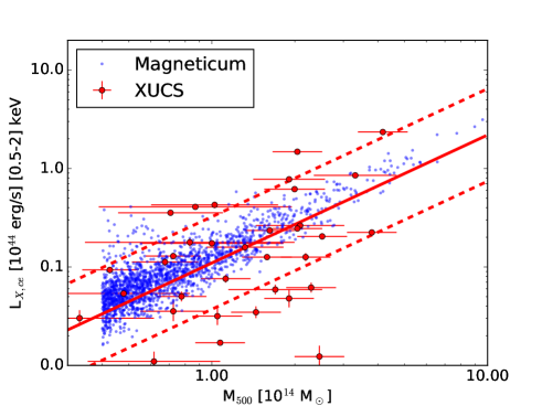
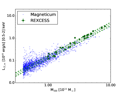
Figure 1: X-ray luminosity in an X-ray unbiased sample (red points, left panel) in the X-ray selected REXCESS sample (green points, right panel) and in the Magneticum simulation (blue points, both panels). Best fit and $\pm 1\sigma$ intrinsic scatter corridors are also shown for the observed data. Photometric errors boost the scatter in the observational data.

2.1 Numerical setup

The Magneticum simulations are based on the N-body code Gadget3, which is an improved version of Gadget2 (Springel et al., 2005b; Springel, 2005; Boylan-Kolchin et al., 2009), with a space-filling curve-aware neighbour search (Ragagnin et al., 2016) and the improved smoothed particle hydrodynamics (SPH) solver from Beck et al. (2016). These simulations include a treatment of radiative cooling, heating, ultraviolet (UV) background, star formation, and stellar feedback processes as in Springel et al. (2005a), connected to a detailed chemical evolution and enrichment model as in Tornatore et al. (2007), which follows 11 chemical elements (H, He, C, N, O, Ne, Mg, Si, S, Ca, and Fe) with the aid of CLOUDY photo-ionisation code (Ferland et al., 1998). Fabjan et al. (2010); Hirschmann et al. (2014) described prescriptions for black hole growth and feedback from AGNs. Haloes and their member galaxies are identified using the friend-of-friend halo finder (Davis et al., 1985) and an improved version of the subhalo finder SUBFIND (Springel et al., 2001), which takes the presence of baryons into account (Dolag et al., 2009). We mainly focus on Magneticum Box2/hr (Hirschmann et al., 2014), covering a length of $\approx 900$ comoving Mpc, with dark matter particle masses $m_{\mathrm{DM}}=9.8\cdot 10^{8}M_{\odot}$ and gas initial particle masses of $m_{\mathrm{gas}}=2\cdot 10^{8}M_{\odot}$ and a gravitational softening of both gas and dark matter of $\epsilon\approx 5$ comoving kpc.

Throughout this paper, we use $R_{\rm 500c}$ and $R_{\rm 200c}$ as halo radii. They are defined to be the radius at which the average density of a galaxy cluster reaches $500$ or $200$ times the critical density of the Universe; see Naderi et al. (2015) for a review of computing masses and radii within a given overdensity.

We extracted all Box2/hr galaxy clusters with $M_{\rm 500c}$ (i.e. the total mass within $R_{\rm 500c}$) greater than $4\times 10^{13}{\rm M}_{\odot}$ at a redshift $z=0$ for a total of $\approx 1800$ galaxy clusters. For each halo, we computed the following quantities: the gas fraction $f_{g},$ from which we removed star-forming particles by considering only particles with $T>3\times 10^{4}K$ and with a cold-gas fraction greater than $0.1;$ the formation redshift $z_{f},$ at which the halo accreted $50\%$ of its final virial mass; The halo concentration $c$, computed by fitting an NFW (Navarro et al., 1997) profile of the average total (i.e. including dark matter and baryons) matter profile over $40$ logarithmically spaced radial bins in the $[0.01-1]R_{\rm{500c}}$ range; the hot-gas temperature $T,$ computed by mass-weighting SPH particle temperatures with the same filter as the gas fraction; the fossilness within $R_{500c},$ which is the stellar mass ratio of the BCG and the most massive satellite (Ragagnin et al., 2019); the richness $n$ of all subhaloes with stellar mass $M_{\star}>3\times 10^{10}M_{\odot};$ the BCG stellar mass $M_{\star,{\rm BCG}},$ as provided by SUBFIND; The core-excised X-ray luminosities $L_{X,{\rm ce}}$ were computed using the APEC model (Smith et al., 2001), which considers the emission of a collisionally ionised, chemically enriched plasma implemented within the external, publicly available package XSPEC (Arnaud, 1996) in the [0.15-1] $R_{\rm 500c}$ range, in the $\left[0.5,2\right]$ keV band. We opted for an $L_{x}$ that was core-excised in order to minimise the impact of details of the sub-grid AGN feedback and of a cool core.

Although fossilness, richness, and BCG mass should correlate with concentration, we decided to include all these indexes in our study because there is no general agreement about the cold-hot baryon correlation in the literature. In this work, all masses and radii are expressed in physical units. They are therefore not implicitly divided by $(1+z)$ or $h_{0}$ as in other works on simulations.

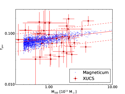
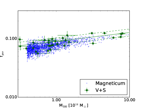
Figure 2: Gas fraction in an X-ray unbiased sample (red points, left panel), in the X-ray selected sample (green points, right panel), and in the Magneticum simulation (blue points, both panels). Best fit and $\pm 1\sigma$ intrinsic scatter corridors are also shown. Photometric errors of the observational samples boost the data scatter.

2.2 Observational data

We compared simulated data against the XUCS and to two X-ray selected samples, REXCESS and an archive sample. XUCS (Paper I) consists of 34 clusters in the very nearby universe ($0.050<z<0.135$) selected from the SDSS spectroscopic survey using more than 50 concordant redshifts whithin 1 Mpc and a velocity dispersion of members $\sigma_{v}>500$ km/s (see Paper I and Andreon et al., 2017b, hereafter Paper II). They are by design in regions of low galactic absorption. There is no X-ray selection in the sample in the sense that the probability of including a cluster is independent of its X-ray luminosity, or any X-ray property, and no cluster is added or removed on the basis of its X-ray luminosity. All clusters were followed up in X-ray with Swift, except for a few with adequate XMM-Newton or Chandra data in the archives. From these data, we derived the X-ray luminosity with a mean error of 0.04 dex (Andreon et al., 2016) and the gas fraction with a mean error of 0.10 dex (Andreon et al., 2017b). The masses were obtained with the caustic technique (Diaferio & Geller, 1997, and later works), which has the advantage of not relying on the dynamical equilibrium hypothesis. The masses have an average mass error of 0.14 dex. In XUCS, caustic masses are consistent with dynamical and weak-lensing masses (Andreon et al. 2016 and Andreon et al. 2017a), and for a single cluster with a deep X-ray follow-up, also with the hydrostatic mass  (Andreon et al., 2019). In other samples, caustic masses are in general found to agree with weak-lensing masses and hydrostatic masses (Geller et al., 2013; Hoekstra et al., 2015; Maughan et al., 2016).

REXCESS (Böhringer et al., 2007) consists of an X-ray selected sample of 33 clusters at low redshift ($z<0.2$) selected from the ROSAT all-sky survey (Truemper, 1993) that was followed up with XMM-Newton. Cluster masses were derived from the Compton $Y_{X}$ parameter (Arnaud et al., 2010), and X-ray luminosities were derived in Pratt et al. (2009). This sample lacks gas-fraction determinations, and therefore we supplemented it with measurements from Vikhlinin et al. (2006) and Sun et al. (2009) (V+S, hereafter). The latter sample was observed with Chandra, has $z<0.25,$ and is formed by 30 clusters and groups, 3 of which are present in both papers, with measurements at $R_{\rm 500c}$. This sample lacks a selection function and uses hydrostatic masses.

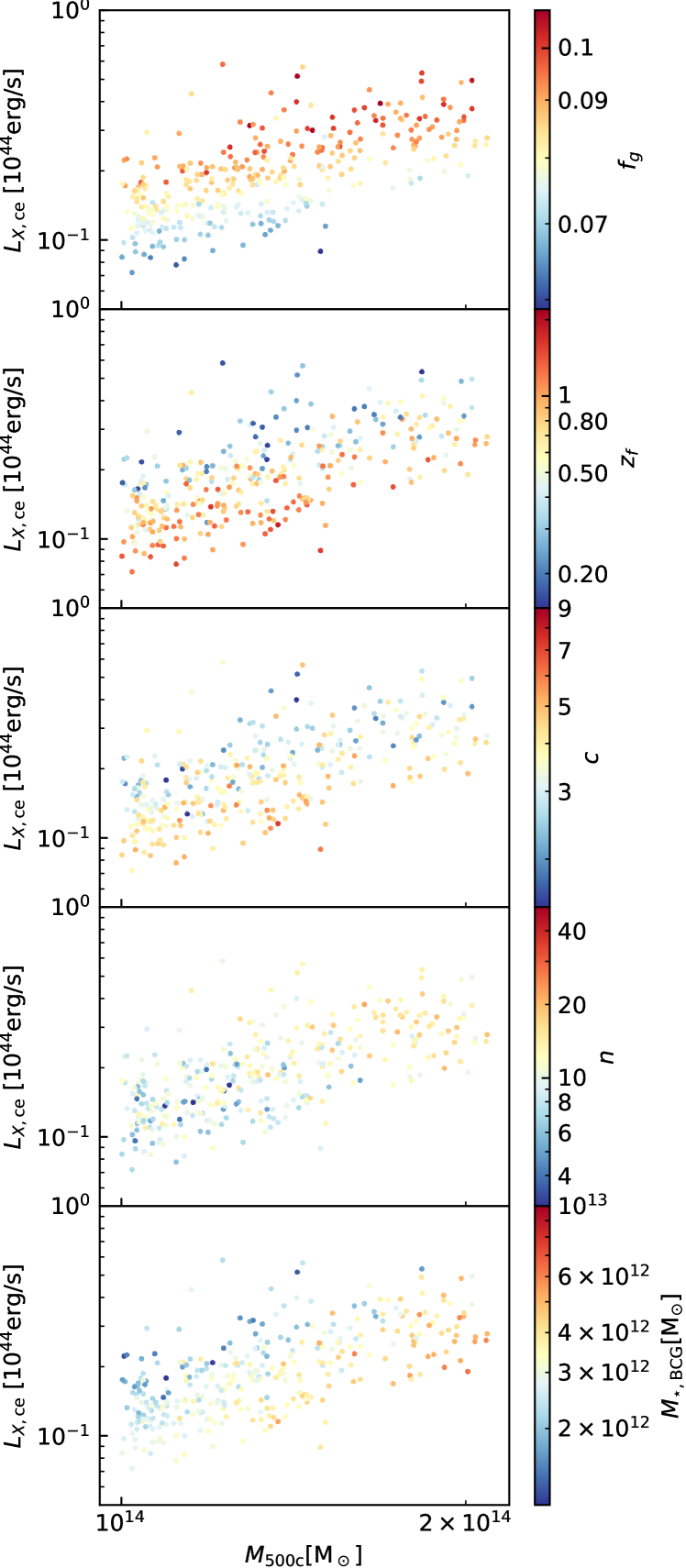
Figure 3: Core-excised X-ray luminosity $L_{X,\rm ce}$ $vs.$ mass $M$ in the Magneticum simulation colour-coded by gas-fraction (top panel), formation epoch $z_{f}$ (second panel from the top), concentration $c$ (central panel), richness $n$ (second panel from the bottom), and BCG stellar mass (bottom panel). To illustrate the dependence at fixed mass, we only show data in a small halo mass range ($1-2\times 10^{14}{\rm M}_{\odot}$).

3 Luminosity-mass relation

In this section we compare the $L_{X}-M$ relation of simulations against the biased and unbiased X-ray samples. Figure 1 shows the relation of $L_{X,ce}$ versus $M_{500c}$ for simulated haloes overplotted on the observed X-ray selected (right panel) and X-ray unbiased (left panel) samples. Simulations and real data share similar slopes (Magneticum: 1.23, XUCS:1.30, and REXCESS: 1.49). The scatter at fixed mass of simulated clusters is between 0.24 dex (at the high-mass end) to 0.30 dex (in the low-mass range), which is smaller than XUCS (0.47 dex), but much larger than REXCESS (0.08 dex).

The Magneticum feedback parameters were calibrated to match observed quantities such as cluster baryon-fractions  (Bocquet et al., 2016) within the uncertainty of the observational data. We therefore do not focus on the exact value of scaling-relation normalisation values, but rather on the scatter at fixed mass.

The Magneticum mean relation has a lower intercept than that of REXCESS because the latter misses clusters with low gas-fractions. The relation is higher than XUCS, however, indicating that gas-poor clusters are more abundant in the Universe than in Magneticum. The larger intercept and lower scatter of X-ray selected samples are known features of samples selected in this way (Andreon et al., 2016). While simulations do not capture the full variety of $L_{X}$ at fixed mass that is observed in XUCS, they offer a spread that is large enough to study the origin of the spread and to characterise gas-poor haloes.

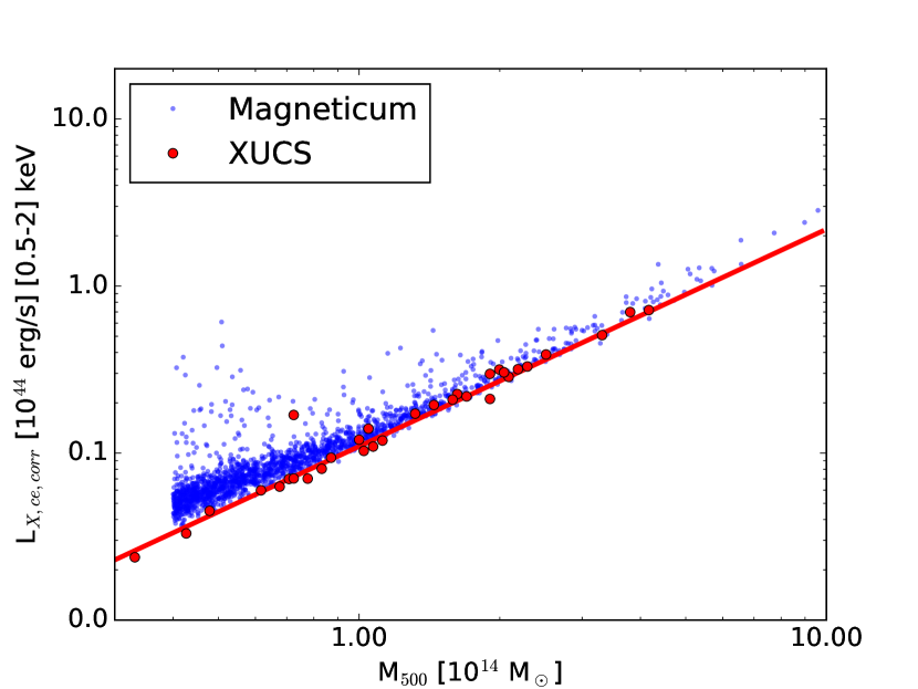
Figure 4: Core-excised X-ray luminosity corrected for gas fraction $L_{X,\rm ce,corr}$ (see Eq. 1) $vs.$ mass $M$. The gas-fraction correction removes most of the scatter around the relation (compare with Fig. 1).

Figure 2 shows the $f_{g}-M$ relation for the simulated data for XUCS and for an X-ray selected sample of relaxed clusters (Vikhlinin et al., 2006; Sun et al., 2009). Simulations and real data share similar slopes (Magneticum: 0.21, and V+S: 0.15; Andreon 2010). The XUCS slope is inherited from that of V+S; see Andreon et al. (2017b). The scatter at fixed mass of the simulated clusters is 0.08 dex (at the high-mass end) to 0.11 dex (in the low-mass range), intermediate between the XUCS intrinsic scatter (0.17 dex), but larger than that of V+S (0.06 dex; Andreon, 2010). The V+S sample has the largest intercept and lowest scatter, which are two known features of samples selected in this way (Andreon et al., 2017b). The Magneticum mean relation has a lower intercept than the X-ray selected sample, but it is higher than XUCS, indicating that clusters are more gas poor in the Universe than in Magneticum. Although the spread at a fixed mass of the simulated data for $L_{X}$ does not exactly match that of XUCS, it is large enough for us to investigate the origin of the spread.

3.1 Dependence on gas fraction, richness, concentration, and formation redshift

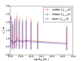
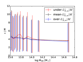
Figure 5: Covariance between formation redshift and X-ray luminosity residuals, with and without gas fraction corrections. Left panel: Formation redshift (16,50,86 percentile) at fixed mass for clusters with $L_{X,ce}$ that is not corrected for gas, split into three tertiles. Middle panel: Formation redshift (16,50,86 percentile) at fixed mass for a cluster with gas-corrected $L_{X,ce}$ split into three tertiles. Right panel: Concentration (16,50,86 percentile) at fixed mass for a cluster with gas-corrected $L_{X,ce}$ split into three tertiles.

Figure 3 shows $L_{X,\rm{ce}}$ versus $M$ of Magneticum galaxy clusters colour-coded by $f_{g}$ (first panel), formation redshift (second panel), concentration (third panel), richness (fourth panel), and BCG stellar mass (fifth panel). The top panel shows that a fixed mass, brighter clusters are gas rich, in agreement with the observational result in Andreon et al. (2017b). They were presented in a similar plot in Andreon et al. (2022). The other panels illustrate that at fixed mass, the X-ray luminosity is correlated to all plotted quantities (blue points are systematically above or below red points), as quantified in Sec. 3.2 : LSB clusters are older (second panel from the top), concentrated (central panel), are less rich (second panel from the bottom), and have more massive BCGs (bottom panel).

Andreon et al. (2017b) showed that the $L_{X}-M$ scatter can be drastically reduced when the X-ray luminosities are corrected for differences in gas fraction; see the red points in Fig. 4 We now determine whether this is true for the simulations as well. For this reason, we defined for each galaxy cluster the $L_{X,\rm{ce}}$ luminosity corrected ($L_{X,\rm{ce,corr}}$) for its $f_{g}$ as

$$L_{X,\rm{ce,corr}}=\left(\dfrac{f_{g}\left(M\right)}{f_{g}}\right)^{2}L_{X,\rm{ce}},$$ (1)

where $f_{g}\left(M\right)$ is the average gas fraction at its mass $M,$ estimated via a linear regression of $\log f_{g}$ versus $\log M$. Fig. 4 shows that the scatter of the luminosity–mass relation is drastically reduced compared to Fig. 1. The scatter decreases from a range of $0.24-0.30$ dex (before correction) to $0.09-0.11$ dex (after correction). It is now readily apparent that the Magneticum and XUCS X-ray $L_{X}-M$ scaling relations are quite similar, but have a slightly different slope and scatter. Nevertheless, both scaling relations become much tighter after the gas fraction is corrected for.

The question is whether all the covariances illustrated in Fig. 3 disappear when gas-fraction corrected X-ray luminosities are employed. Sec. 3.2 quantitatively addresses this point, but we illustrate the effect of the gas-fraction correction on the concentration and formation redshift here. When the clusters are split into tertilies of X-ray luminosities at fixed mass, LSB clusters have older formation times (left panel of figure 5). However, when we use tertiles of X-ray corrected luminosities ($L_{X,\rm{ce,corr}}$), then the formation times (central panel) and concentration (right panel) show no covariance with $L_{X,\rm{ce,corr}}.$

3.2 Full covariance analysis

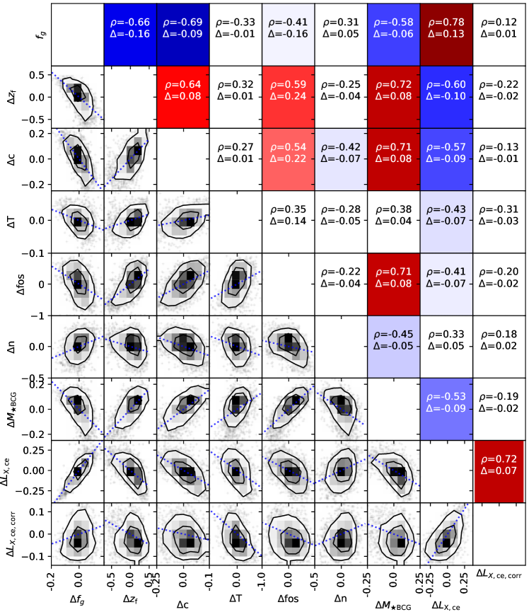
Figure 6: Correlation between cluster properties. Lower triangle: Scatter plot of the residuals at fixed halo mass $M_{500c}$ of $\log_{10}$ gas fraction $f_{g},$ $\log_{10}$ formation redshift $z_{f},$ $\log_{10}$ concentration $c$, $\log_{10}$ temperature, $\log_{10}$ fossilness, $\log_{10}$ richness $n,$ $\log_{10}$ X-ray luminosity, and $\log_{10}$ $f_{g}^{2}$ corrected luminosity (as in Eq. 1). The dotted lines show the slope for individual correlation coefficients. When it points in a direction different from the data elongation, it indicates that the data do not satisfy the assumption for the derivation of the correlation coefficient. The upper triangle shows the corresponding correlation coefficient $\rho$ and the amplitude of the covariance $\Delta$.

To study the covariance at fixed mass, we performed a linear regression of the logarithm of each property ($f_{g},z_{f},c,T,$ fossilness, $n,M_{\star\rm BCG},L_{\rm X,ce},$ and $L_{\rm X,ce,corr}$) against $\log$M, and we searched for covariance in the residuals from the mean relation. Fig. 6 shows the correlation coefficient $\rho$ (upper triangle) and residual scatter (lower triangle) plots. The first is a measure of the linear correlation between residuals, and gives the fraction of the ordinate scatter explained by the abscissa scatter given the linear slope $s$ for individual correlation coefficients, $s=\rho\sigma_{y}/\sigma_{x}.$ This is shown as the dashed line in the lower triangle plots. The lower triangle plots illustrate whether the linearity hypothesis is plausible, and also whether the trend is of any physical significance: a correlation involving a negligible change is unlikely to be of any physical interest, even if it is statistically significant. We quantify the above with the ordinate variation when the abscissa changes by $1\sigma$, $\Delta=s\sigma_{x}=\rho\sigma_{y}$, whose values are reported in the upper triangle.

Values of $\Delta<0.05$ (i.e. $\sim 10$% differences) are hardly accessible with observations of individual objects in the large samples needed for covariance studies, whereas correlations $\rho<0.3$ often result from assumptions that are not satisfied by the data. The richness-temperature covariance for example is vertically elongated, but the correlation coefficient indicates an elongation of 45 degree away from it (see Fig 6). These correlation coefficients should be considered with caution.

Fig. 6 confirms the tight correlation at fixed mass of the core-excised X-ray luminosity with gas-fraction (i.e. that gas-poor clusters are also X-ray faint; this covariance has the highest correlation coefficient, 0.78), with formation redshift (i.e, that these X-ray faint clusters formed early) and with concentration (i.e. that X-ray faint clusters have a high concentration).

The values of $L_{X,\rm{ce,corr}}$ show little or no covariance with any other property ($\rho\lesssim 0.3$), as already found in the previous section for some of these quantities. Thus the gas-fraction correction absorbs most of the scatter in all the considered scaling relations.

This is remarkable because this correction was motivated by removing covariance with one quantity, gas fraction, not with the remaining six quantities. The disappearance of these correlations indicates a common origin for the residuals from the mass trend, that is, that the physical reason for the differences in gas fraction also likely causes deviations from the other quantities from the mean relation.

Out of the remaining quantities, three of the largest covariances are with BGC stellar mass ($vs.$ with formation redshift, concentration, and fossilness) in the sense that clusters of a given mass with more massive BCGs also have a higher-than-average formation redshift and a higher-than-average concentration. We interpret this result as due to the longer time that the BCG had to assimilate more satellites (Ragagnin et al., 2019). Fossilness, concentration, and formation time show strong covariance (Ragagnin et al., 2019). Finally, gas fraction and formation times are anti-correlated, which may impact observational studies that constrain cosmological parameters with gas fraction (e.g. Ettori et al., 2003; Mantz et al., 2022). Interestingly, richness shows low levels of covariance ($\Delta$) with formation redshift, gas fraction, and a weak correlation with concentration and mass of the BCG. This confirms that it can be a very useful mass proxy with little sensitivity to the mass accretion history, differently from, for instance, gas fraction or X-ray luminosity. Of the considered quantities, the temperature ist less covariant with the others: all correlation values are below $\approx 0.4,$ and some of the covariances (with gas fraction, concentration, and gas fraction) are hardly observable at best. The source of the temperature variance therefore appears to be unrelated to the others we considered.

4 Discussion

4.1 Comparison with observations and previous simulations

Our analysis extends previous simulation works that investigated one or just a few covariance quantities (Wechsler et al., 2002; Zhao et al., 2003; Lu et al., 2006; Ragone-Figueroa et al., 2010; Cui et al., 2011; Angulo et al., 2012; Giocoli et al., 2012; Ragagnin et al., 2019; Bose et al., 2019; Anbajagane et al., 2020; Wang et al., 2020; Richardson & Corasaniti, 2021) by addressing a larger set of variables that is analysed with a single numerical technique. Moreover, we tested the finding of recent observational studies (Andreon et al., 2017b) that most of the scatter of the $L_{x}-M$ relation can be absorbed by correcting $L_{x}$ for $f_{g}^{2}.$

In observational studies, Farahi et al. (2019) (that focuses on the most massive clusters), found a negative correlation between hot ($f_{g}$) and cold (richness) baryons at fixed mass, unlike Puddu & Andreon (2022), who used XUCS clusters. Our simulated data agree with Puddu & Andreon (2022) that gas fraction and richness show a positive correlation. However, the way in which Puddu & Andreon (2022) computed richnesses differs from our way. The authors counted galaxies within a cylinder, not a sphere, and used a slightly higher galaxy mass threshold.

On the other hand, Puddu & Andreon (2022) reported that LSB clusters have fainter BCGs and a slightly smaller magnitude gap ($\Delta M_{1,2}$ between the central and the brightest satellite), while the Magneticum simulation shows an opposite trend according to which gas-poor clusters are old (see Fig. 6) and have brighter BCGs, because the BCG had time to accrete more satellites (as in Fig. 7 and Fig. 8 in Ragagnin et al., 2019). We emphasise, however, that separating the BCG luminosity from intracluster light is challenging and that different methods have been used to address this problem in simulations and observations.

Gas-poor clusters have a high concentration in simulations on average (with some scatter, see Fig. 6). CL2015 (Andreon et al., 2019) is a gas-poor galaxy cluster with a low concentration. Although it does not follow the average trend seen in simulation, it lies within the $1\sigma$ scatter of it.

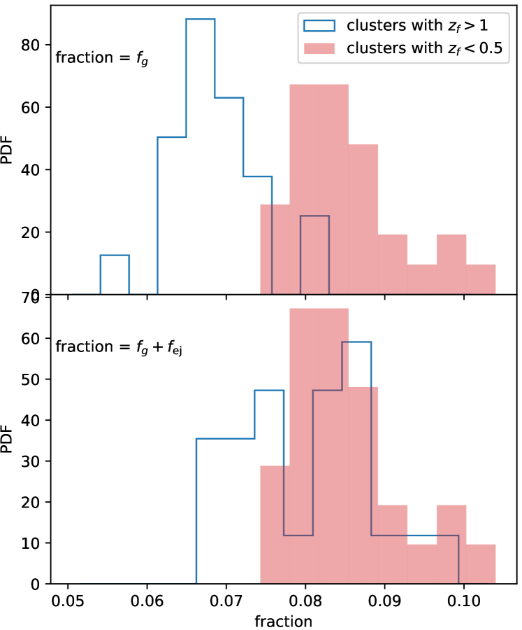
Figure 7: PDF of gas fraction for old clusters ($z_{f}>1$, with blue steps) and young clusters ($z_{f}<0.5$, as pink shaded area). The top panel shows the gas-fraction within $R_{\rm 500c}$ and the bottom panel shows the gas-fraction within $R_{\rm 500c}$ corrected with the amount of gas that was inside the halo at formation time and have been ejected outside outside the virial radius ($f_{\rm ej}$). In both cases we consider haloes in the range of mass $M_{\rm 200c}\in[1-2]\times 10^{14}M_{\odot}.$ We see that the amount of ejected gas accounts for much of the difference in $f_{g}$ between old and young clusters.

4.2 Role of AGN outflow

Full-physics simulations and processes such as AGN feedback proved to significantly impact galaxy cluster mass profiles up to their outskirts  (Duffy et al., 2010; Fabjan et al., 2011; Velliscig et al., 2014), to lower the gas fraction, to strongly suppress star formation galaxies (Bower et al., 2017), and to boost the X-ray luminosity during mergers (see e.g. Torri et al., 2004; Poole et al., 2007).

Feedback from AGN in particular is capable of ejecting a significant fraction of gas outside the halo (Davies et al., 2020). We studied whether AGN feedback is the reason that older clusters are gas poor. To this end, we selected clusters in the range of $M_{\rm 200c}\in[1-2]\times 10^{14}{\rm M}_{\odot}$ and followed gas particles in time that were inside the virial radius at formation time.

Fig. 7 (top panel) shows that the gas fraction of old clusters ($z_{f}>1,$ blue histogram) is lower than for young clusters ($z_{f}<0.5,$ pink shaded histogram). The difference is mainly due to gas that was within the virial radius at formation time and that was later ejected ($f_{\rm ej}$). When the ejected gas is returned, the two distributions approach each other (bottom panel of Fig. 7)

The increase in $f_{g}$ that we find between the top and bottom panels of Fig. 7 is not an artefact because $\rho_{c}$ changes with time (which enters in the definition of $R_{\rm 200c}$). $\rho_{c}$ decreases with time, and the baryon fraction of the material that is accreted by clusters is similar to the cosmic baryon fraction (see Sec. 4.3 in Vallés-Pérez et al., 2020). Moreover, the conversion of gas into stars plays a negligible role, as we estimated that the fraction of stars that is produced after formation time is $<5\%$ of the galaxy cluster final masses at $z=0$.

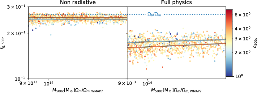
Figure 8: Gas fraction $f_{g}$ $vs.$ halo mass $M_{\rm 500c}$ for Magneticum Box1a/mr non-radiative run (left panel) and full-physics run (right panel). Points are colour-coded by concentration within $R_{\rm 500c}.$ Lines show the average gas fraction for the two quantiles in gas concentration, up to $16\%$ in blue, and from $85\%$ in red, both coloured according to their average concentration. The non-radiative simulation shows a slight dependence of concentration on gas fraction, while full-physics runs show the opposite behaviour: the gas fraction is anti-correlated with concentration. Masses are corrected to WMAP7 $\Omega_{m}$ for consistency with the other results of this study.

4.3 Role of baryon physics in the gas fraction versus concentration covariance

In this subsection we rule out the possibility that the correlation between gas fraction and formation redshift is due to environmental effects in older galaxy clusters. To this end, we studied the relation between gas fraction and concentration (which correlates with formation redshift) at fixed mass by comparing a non-radiative run with a full-physics run. We do not have a WMAP7 non-radiative counterpart; therefore we compared two Magneticum Box1a/mr simulations with cosmological parameters $\Omega_{m}=0.153,\Omega_{b}=0.0408,\sigma_{8}=0.614,$ and $h_{0}=0.666.$

Figure 8 shows $f_{g}$ as a function of halo mass colour-coded by halo concentration taken from Ragagnin et al. (2021). In the non-radiative run, the gas-fraction is close to the cosmic gas fraction $\Omega_{b}/\Omega_{m},$ while full-physics simulations have much lower $f_{g}$, in agreement with previous studies (Eckert et al., 2011; Planelles et al., 2013), which showed that this difference is due to the AGN feedback, because the ejected gas is capable of escaping from clusters. The non-radiative simulation $f_{g}-M$ relation has an indication of an anti-correlation with concentration at most, that is, gas-rich clusters tend to be concentrated (left panel), as opposed to the full-physics run (right panel). We can speculate that in non-radiative simulations, due to the lack of AGN feedback, the process of adiabatic contraction brings more gas to the center as the dark matter halo becomes more concentrated. This experiment shows that very different baryon-physics prescriptions can reverse the correlation between $c$ and $f_{g},$ which explains why the Stanek et al. (2010) simulations and modern simulations reported contrasting results.

5 Conclusion

We characterised the origin of LSB and gas-poor galaxy clusters in cosmological simulations by analysing several haloes from the Magneticum simulations. . We found a strong covariance between the X-ray luminosity and the gas fraction at fixed mass, in agreement with recent studies of unbiased samples (XUCS) from Puddu & Andreon (2022), and following the reasoning in Andreon et al. (2017b) that the X-ray luminosity scales with $f_{g}^{2}$ at fixed halo mass, we were able to remove the X-ray intrinsic scatter by applying a gas-fraction correction in both simulations and observations (see our Fig. 4). In particular, correcting the luminosity for $f_{g}^{2}$ reduced all our correlation coefficients to almost zero (see last column in Fig. 6).

We then characterised LSB and gas-poor galaxy clusters and found them to be older, with a higher concentration, and with a slight anti-correlation with richness and tested whether the feedback mechanism lowers the gas fraction of older clusters. To this end, we quantified the amount of depleted gas at formation time and found that older clusters depleted more gas and that the amount of depleted gas is enough to justify their low gas fraction (compared to gas-rich systems in a fixed mass bin). Finally, we ruled out the hypothesis that the environment of older clusters caused them to be gas poor. To do this, we compared full-physics simulations against non-radiative simulations, and we found that the latter do not show any negative correlation between gas fraction and concentration (which strongly correlates with formation redshift). We therefore conclude that older galaxy clusters tend to be gas poor (and thus LSB) because the feedback mechanism depleted a significant amount of gas from these systems.

Data availability

Raw simulation data were generated at the C²PAP/LRZ cosmology simulation web portal https://c2papcosmosim.uc.lrz.de/. The derived data supporting the findings of this study are available from the corresponding author AR on request. The derived data supporting the findings of this study are available from the corresponding author SA on request.

References

- Allen et al. (2011) Allen, S. W., Evrard, A. E., & Mantz, A. B. 2011, ARA&A, 49, 409
- Anbajagane et al. (2020) Anbajagane, D., Evrard, A. E., Farahi, A., et al. 2020, MNRAS, 495, 686
- Andreon (2010) Andreon, S. 2010, MNRAS, 407, 263
- Andreon et al. (2016) Andreon, S., Dong, H., & Raichoor, A. 2016, A&A, 593, A2
- Andreon & Moretti (2011) Andreon, S. & Moretti, A. 2011, A&A, 536, A37
- Andreon et al. (2019) Andreon, S., Moretti, A., Trinchieri, G., & Ishwara-Chandra, C. H. 2019, A&A, 630, A78
- Andreon et al. (2022) Andreon, S., Trinchieri, G., & Moretti, A. 2022, MNRAS, 511, 4991
- Andreon et al. (2017a) Andreon, S., Trinchieri, G., Moretti, A., & Wang, J. 2017a, A&A, 606, A25
- Andreon et al. (2017b) Andreon, S., Wang, J., Trinchieri, G., Moretti, A., & Serra, A. L. 2017b, A&A, 606, A24
- Angulo et al. (2012) Angulo, R. E., Springel, V., White, S. D. M., et al. 2012, MNRAS, 426, 2046
- Arnaud (1996) Arnaud, K. A. 1996, in Astronomical Society of the Pacific Conference Series, Vol. 101, Astronomical Data Analysis Software and Systems V, ed. G. H. Jacoby & J. Barnes, 17
- Arnaud et al. (2010) Arnaud, M., Pratt, G. W., Piffaretti, R., et al. 2010, A&A, 517, A92
- Beck et al. (2016) Beck, A. M., Murante, G., Arth, A., et al. 2016, MNRAS, 455, 2110
- Beltz-Mohrmann & Berlind (2021) Beltz-Mohrmann, G. D. & Berlind, A. A. 2021, ApJ, 921, 112
- Bertocco et al. (2020) Bertocco, S., Goz, D., Tornatore, L., et al. 2020, in Astronomical Society of the Pacific Conference Series, Vol. 527, Astronomical Society of the Pacific Conference Series, ed. R. Pizzo, E. R. Deul, J. D. Mol, J. de Plaa, & H. Verkouter, 303
- Biffi et al. (2013) Biffi, V., Dolag, K., & Böhringer, H. 2013, MNRAS, 428, 1395
- Bocquet et al. (2016) Bocquet, S., Saro, A., Dolag, K., & Mohr, J. J. 2016, MNRAS, 456, 2361
- Bode et al. (2009) Bode, P., Ostriker, J. P., & Vikhlinin, A. 2009, ApJ, 700, 989
- Böhringer et al. (2007) Böhringer, H., Schuecker, P., Pratt, G. W., et al. 2007, A&A, 469, 363
- Bose et al. (2019) Bose, S., Eisenstein, D. J., Hernquist, L., et al. 2019, MNRAS, 490, 5693
- Bower et al. (2017) Bower, R. G., Schaye, J., Frenk, C. S., et al. 2017, MNRAS, 465, 32
- Boylan-Kolchin et al. (2009) Boylan-Kolchin, M., Springel, V., White, S. D. M., Jenkins, A., & Lemson, G. 2009, MNRAS, 398, 1150
- Castro et al. (2021) Castro, T., Borgani, S., Dolag, K., et al. 2021, MNRAS, 500, 2316
- Corasaniti et al. (2021) Corasaniti, P.-S., Sereno, M., & Ettori, S. 2021, ApJ, 911, 82
- Crain et al. (2007) Crain, R. A., Eke, V. R., Frenk, C. S., et al. 2007, MNRAS, 377, 41
- Cui et al. (2011) Cui, W., Springel, V., Yang, X., De Lucia, G., & Borgani, S. 2011, MNRAS, 416, 2997
- Davies et al. (2020) Davies, J. J., Crain, R. A., Oppenheimer, B. D., & Schaye, J. 2020, MNRAS, 491, 4462
- Davis et al. (1985) Davis, M., Efstathiou, G., Frenk, C. S., & White, S. D. M. 1985, ApJ, 292, 371
- Diaferio & Geller (1997) Diaferio, A. & Geller, M. J. 1997, ApJ, 481, 633
- Dolag et al. (2009) Dolag, K., Borgani, S., Murante, G., & Springel, V. 2009, MNRAS, 399, 497
- Dolag et al. (2015) Dolag, K., Gaensler, B. M., Beck, A. M., & Beck, M. C. 2015, MNRAS, 451, 4277
- Dolag et al. (2016) Dolag, K., Komatsu, E., & Sunyaev, R. 2016, MNRAS, 463, 1797
- Duffy et al. (2010) Duffy, A. R., Schaye, J., Kay, S. T., et al. 2010, MNRAS, 405, 2161
- Dvorkin & Rephaeli (2015) Dvorkin, I. & Rephaeli, Y. 2015, MNRAS, 450, 896
- Eckert et al. (2011) Eckert, D., Molendi, S., & Paltani, S. 2011, A&A, 526, A79
- Ettori et al. (2006) Ettori, S., Dolag, K., Borgani, S., & Murante, G. 2006, MNRAS, 365, 1021
- Ettori et al. (2003) Ettori, S., Tozzi, P., & Rosati, P. 2003, A&A, 398, 879
- Fabjan et al. (2011) Fabjan, D., Borgani, S., Rasia, E., et al. 2011, MNRAS, 416, 801
- Fabjan et al. (2010) Fabjan, D., Borgani, S., Tornatore, L., et al. 2010, MNRAS, 401, 1670
- Farahi et al. (2019) Farahi, A., Mulroy, S. L., Evrard, A. E., et al. 2019, Nature Communications, 10, 2504
- Ferland et al. (1998) Ferland, G. J., Korista, K. T., Verner, D. A., et al. 1998, PASP, 110, 761
- Gaspari et al. (2020) Gaspari, M., Tombesi, F., & Cappi, M. 2020, Nature Astronomy, 4, 10
- Geller et al. (2013) Geller, M. J., Diaferio, A., Rines, K. J., & Serra, A. L. 2013, ApJ, 764, 58
- Giocoli et al. (2012) Giocoli, C., Tormen, G., & Sheth, R. K. 2012, MNRAS, 422, 185
- Giodini et al. (2013) Giodini, S., Lovisari, L., Pointecouteau, E., et al. 2013, Space Sci. Rev., 177, 247
- Hirschmann et al. (2014) Hirschmann, M., Dolag, K., Saro, A., et al. 2014, MNRAS, 442, 2304
- Hoekstra et al. (2015) Hoekstra, H., Herbonnet, R., Muzzin, A., et al. 2015, MNRAS, 449, 685
- Hoekstra et al. (2012) Hoekstra, H., Mahdavi, A., Babul, A., & Bildfell, C. 2012, MNRAS, 427, 1298
- Hudson et al. (2010) Hudson, D. S., Mittal, R., Reiprich, T. H., et al. 2010, A&A, 513, A37
- Khoraminezhad et al. (2021) Khoraminezhad, H., Lazeyras, T., Angulo, R. E., Hahn, O., & Viel, M. 2021, J. Cosmology Astropart. Phys., 2021, 023
- Komatsu et al. (2011) Komatsu, E., Smith, K. M., Dunkley, J., et al. 2011, ApJS, 192, 18
- Kravtsov & Borgani (2012) Kravtsov, A. V. & Borgani, S. 2012, ARA&A, 50, 353
- Lima & Hu (2005) Lima, M. & Hu, W. 2005, Phys. Rev. D, 72, 043006
- Lu et al. (2006) Lu, Y., Mo, H. J., Katz, N., & Weinberg, M. D. 2006, MNRAS, 368, 1931
- Ludlow et al. (2012) Ludlow, A. D., Navarro, J. F., Li, M., et al. 2012, MNRAS, 427, 1322
- Mantz et al. (2022) Mantz, A. B., Morris, R. G., Allen, S. W., et al. 2022, MNRAS, 510, 131
- Maughan et al. (2016) Maughan, B. J., Giles, P. A., Rines, K. J., et al. 2016, MNRAS, 461, 4182
- Melchior et al. (2015) Melchior, P., Suchyta, E., Huff, E., et al. 2015, MNRAS, 449, 2219
- Naderi et al. (2015) Naderi, T., Malekjani, M., & Pace, F. 2015, MNRAS, 447, 1873
- Navarro et al. (1997) Navarro, J. F., Frenk, C. S., & White, S. D. M. 1997, ApJ, 490, 493
- Okabe et al. (2010) Okabe, N., Zhang, Y. Y., Finoguenov, A., et al. 2010, ApJ, 721, 875
- Ostriker et al. (2005) Ostriker, J. P., Bode, P., & Babul, A. 2005, ApJ, 634, 964
- Pacaud et al. (2007) Pacaud, F., Pierre, M., Adami, C., et al. 2007, MNRAS, 382, 1289
- Planelles et al. (2013) Planelles, S., Borgani, S., Dolag, K., et al. 2013, MNRAS, 431, 1487
- Poole et al. (2007) Poole, G. B., Babul, A., McCarthy, I. G., et al. 2007, MNRAS, 380, 437
- Pratt et al. (2009) Pratt, G. W., Croston, J. H., Arnaud, M., & Böhringer, H. 2009, A&A, 498, 361
- Puddu & Andreon (2022) Puddu, E. & Andreon, S. 2022, MNRAS, 511, 2968
- Ragagnin et al. (2017) Ragagnin, A., Dolag, K., Biffi, V., et al. 2017, Astronomy and Computing, 20, 52
- Ragagnin et al. (2019) Ragagnin, A., Dolag, K., Moscardini, L., Biviano, A., & D’Onofrio, M. 2019, MNRAS, 486, 4001
- Ragagnin et al. (2021) Ragagnin, A., Saro, A., Singh, P., & Dolag, K. 2021, MNRAS, 500, 5056
- Ragagnin et al. (2016) Ragagnin, A., Tchipev, N., Bader, M., Dolag, K., & Hammer, N. J. 2016, in Advances in Parallel Computing, Volume 27: Parallel Computing: On the Road to Exascale, Edited by Gerhard R. Joubert, Hugh Leather, Mark Parsons, Frans Peters, Mark Sawyer. IOP Ebook, ISBN: 978-1-61499-621-7, pages 411-420
- Ragone-Figueroa et al. (2010) Ragone-Figueroa, C., Plionis, M., Merchán, M., Gottlöber, S., & Yepes, G. 2010, MNRAS, 407, 581
- Remus et al. (2017) Remus, R.-S., Dolag, K., Naab, T., et al. 2017, MNRAS, 464, 3742
- Richardson & Corasaniti (2021) Richardson, T. R. G. & Corasaniti, P. S. 2021, arXiv e-prints, arXiv:2112.04926
- Saro et al. (2014) Saro, A., Liu, J., Mohr, J. J., et al. 2014, MNRAS, 440, 2610
- Schrabback et al. (2021) Schrabback, T., Bocquet, S., Sommer, M., et al. 2021, MNRAS, 505, 3923
- Singh et al. (2020) Singh, P., Saro, A., Costanzi, M., & Dolag, K. 2020, MNRAS, 494, 3728
- Smith et al. (2001) Smith, R. K., Brickhouse, N. S., Liedahl, D. A., & Raymond, J. C. 2001, ApJ, 556, L91
- Springel (2005) Springel, V. 2005, MNRAS, 364, 1105
- Springel et al. (2005a) Springel, V., Di Matteo, T., & Hernquist, L. 2005a, MNRAS, 361, 776
- Springel et al. (2005b) Springel, V., White, S. D. M., Jenkins, A., et al. 2005b, Nature, 435, 629
- Springel et al. (2001) Springel, V., White, S. D. M., Tormen, G., & Kauffmann, G. 2001, MNRAS, 328, 726
- Stanek et al. (2010) Stanek, R., Rasia, E., Evrard, A. E., Pearce, F., & Gazzola, L. 2010, ApJ, 715, 1508
- Steinborn et al. (2016) Steinborn, L. K., Dolag, K., Comerford, J. M., et al. 2016, MNRAS, 458, 1013
- Steinborn et al. (2015) Steinborn, L. K., Dolag, K., Hirschmann, M., Prieto, M. A., & Remus, R.-S. 2015, MNRAS, 448, 1504
- Stern et al. (2019) Stern, C., Dietrich, J. P., Bocquet, S., et al. 2019, MNRAS, 485, 69
- Sun et al. (2009) Sun, M., Voit, G. M., Donahue, M., et al. 2009, ApJ, 693, 1142
- Taffoni et al. (2020) Taffoni, G., Becciani, U., Garilli, B., et al. 2020, in Astronomical Society of the Pacific Conference Series, Vol. 527, Astronomical Society of the Pacific Conference Series, ed. R. Pizzo, E. R. Deul, J. D. Mol, J. de Plaa, & H. Verkouter, 307
- Teklu et al. (2015) Teklu, A. F., Remus, R.-S., Dolag, K., et al. 2015, ApJ, 812, 29
- Tornatore et al. (2007) Tornatore, L., Borgani, S., Dolag, K., & Matteucci, F. 2007, Monthly Notices of the Royal Astronomical Society, 382, 1050
- Torri et al. (2004) Torri, E., Meneghetti, M., Bartelmann, M., et al. 2004, MNRAS, 349, 476
- Truemper (1993) Truemper, J. 1993, Science, 260, 1769
- Truong et al. (2018) Truong, N., Rasia, E., Mazzotta, P., et al. 2018, MNRAS, 474, 4089
- Vallés-Pérez et al. (2020) Vallés-Pérez, D., Planelles, S., & Quilis, V. 2020, MNRAS, 499, 2303
- van de Sande et al. (2019) van de Sande, J., Lagos, C. D. P., Welker, C., et al. 2019, MNRAS, 484, 869
- Velliscig et al. (2014) Velliscig, M., van Daalen, M. P., Schaye, J., et al. 2014, MNRAS, 442, 2641
- Vikhlinin et al. (2006) Vikhlinin, A., Kravtsov, A., Forman, W., et al. 2006, ApJ, 640, 691
- Wang et al. (2020) Wang, K., Mao, Y.-Y., Zentner, A. R., et al. 2020, MNRAS, 498, 4450
- Wechsler et al. (2002) Wechsler, R. H., Bullock, J. S., Primack, J. R., Kravtsov, A. V., & Dekel, A. 2002, ApJ, 568, 52
- Wechsler & Tinker (2018) Wechsler, R. H. & Tinker, J. L. 2018, ARA&A, 56, 435
- Xu et al. (2018) Xu, W., Ramos-Ceja, M. E., Pacaud, F., Reiprich, T. H., & Erben, T. 2018, A&A, 619, A162
- Zhao et al. (2003) Zhao, D. H., Mo, H. J., Jing, Y. P., & Börner, G. 2003, MNRAS, 339, 12